如果你也在 怎样代写理论力学theoretical mechanics这个学科遇到相关的难题，请随时右上角联系我们的24/7代写客服。

理论力学主要研究物体的力学性能及运动规律，是力学的基础学科，由静力学、运动学和动力学三大部分组成。也有人认为运动学是动力学的一部分，而提出二分法。

statistics-lab™ 为您的留学生涯保驾护航 在代写理论力学theoretical mechanics方面已经树立了自己的口碑, 保证靠谱, 高质且原创的统计Statistics代写服务。我们的专家在代写理论力学theoretical mechanics代写方面经验极为丰富，各种代写理论力学theoretical mechanics相关的作业也就用不着说。

我们提供的理论力学theoretical mechanics及其相关学科的代写，服务范围广, 其中包括但不限于:

• Statistical Inference 统计推断
• Statistical Computing 统计计算
• Advanced Probability Theory 高等概率论
• Advanced Mathematical Statistics 高等数理统计学
• (Generalized) Linear Models 广义线性模型
• Statistical Machine Learning 统计机器学习
• Longitudinal Data Analysis 纵向数据分析
• Foundations of Data Science 数据科学基础

物理代写|理论力学代写theoretical mechanics代考|Results of the Measurements

The amplitude characteristics are presented in the Table 2. The analysis of the obtained data shows that obvious filtration properties of first, second and third samples begin after the frequency $0.6 \mathrm{MHz}$. The increase of the distance between the rows, used in the third sample, has no effect on the through-transmitted amplitude in the latter case; however an obvious change of the impulse shape is quite clear, much more notable than for the first two samples. One may conclude that the increase in the distance between the rows complicated the diffraction field inside the sample. The fourth sample begins to demonstrate its filtration properties just at the frequency of $0.4 \mathrm{MHz}$, that is obviously connected with smaller ratio of the US wave length above the size of the obstacle.

The preliminary investigations $[1,2]$ show that after the first filtration strip there is a strip of almost perfect transmission. As can be seen from Fig. 5 and Table 2, for the first three samples such a frequency strip begins from $1.8 \mathrm{MHz}$. This effect is less pronounced for the fourth sample, though the amplitude of the through-transmitted signal is still higher than at the frequency $1.25 \mathrm{MHz}$.

Analyzing the table, one may conclude that the increase of the size of the holes (the fourth sample) results in the worst through-transmission in the meta-material, cutting off more than $90 \%$ of energy, beginning from the frequency $-1 \mathrm{MHz}$. The increase of the distance between the rows along the wave propagation also reduces the carrying capacity for higher frequencies, and the passage to the first filtration band becomes smoother (which is obvious for the frequency equal to $0.6 \mathrm{MHz}$, where the sample 3 demonstrates the best through-transmission). The shift of the rows in the second sample has not so strong effect at low frequencies, and in some cases even improves the through-transmission of the US signal, as can be seen for example, for the frequency $1.25 \mathrm{MHz}$. Nevertheless, for higher frequencies one can see a significant suppression of the transmission, which may be connected with a complex structure of the re-reflections inside the meta-material.

物理代写|理论力学代写theoretical mechanics代考|Simulation Method Using the Wang-Landau Algorithm

Monte-Carlo method use broad class of computational algorithms which are based on random walks. The typical problem in statistical physics that can be solved by these method is calculating mean values of macroscopic variables (energy, order parameter,

etc.) at different temperatures for systems which follows Boltzmann statistics. There are some techniques for Monte-Carlo method: Metropolis [18], Wolff [19], Lee [20], Wang-Landau algorithms [21], parallel tempering [22]. In this section, Metropolis and Wang-Landau algorithms are described and illustrated on the example of twodimensional Ising model.

The Ising model consists of spins which have two possible orientations. Originally developed for simulation of ferromagnetic materials, now, this model has many applications including the simulation of ferroelectrics [23], spin glasses [24], image data processing [25], neuroscience, etc. In 1944 , the two-dimensional Ising model on a square lattice was analytically solved by Onsager [26]. The Hamiltonian of this model is determined by the formula:
$$
E=-J \sum_{\langle i, j\rangle} \overrightarrow{S_{i}} \overrightarrow{S_{j}}-\vec{H} \sum_{i} \overrightarrow{S_{i}}
$$
where $\overrightarrow{S_{i}}$ is the value of spin located in site $i$, the symbol $\langle i, j\rangle$ denotes the pairs of nearest-neighbor segments, $J$ is a parameter of spin interactions, $\vec{H}$ is the external magnetic field strength.

The Metropolis algorithm generates the sequence of states at a predetermined temperature using the probability distribution for the system. For the Ising model, the Metropolis algorithm should be applied as follows:

1. A random spin is chosen and rotated.
2. The new system configuration is accepted with probability:
   $$
   P=\min \left(-\frac{\Delta E}{k_{\mathbb{B}} T}, 1\right),
   $$
   where $\Delta E$ is energy change due to the spin rotation, $k_{B}$ is the Boltzmann constant, $T$ is the temperature.
3. Steps 1 and 2 are repeated.
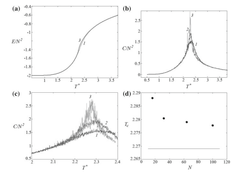
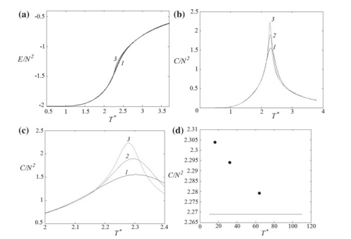
   The results of simulation for the two-dimensional Ising model with periodic boundary conditions obtained by means of the Metropolis algorithm are presented in Fig. 1. The heat capacity was determined by the formula:
   $$
   C=\frac{\left\langle E^{2}\right\rangle-\langle E\rangle^{2}}{k_{B} T^{2}} .
   $$

物理代写|理论力学代写theoretical mechanics代考|Investigation of the Influence of Bulk Properties

The surface properties of layers are determined not only by chemical composition of the substance, but also by their physical structure and the orientational order of polymer chains [29]. Intermolecular orientation interactions are much weaker than valence interactions; therefore, the self-organization of the system with the given chemical structure is determined by intermolecular interactions. In this chapter, we consider the equilibrium properties and phase transitions on the surface of ferroelectric polymer system, in which orientational interactions both between the surface molecules and molecules located in the bulk are taken into account.

Model. Usually, polymer chains have predominantly planar orientation relatively to the interphase boundary [30]. Therefore, in this paper, to describe the surface of ferroelectric polymer systems, we use a two-dimensional model, which consist of $M$ freely-jointed chains, each of which is a sequence of $N$ connected rigid segments, located in parallel to the surface (Fig. 4).

The main quantitative characteristic of the polymer chain flexibility is the persistent length $a$, which is related with the energetic constant of intrachain orientation interaction $K_{1}$ by the ratio:
$$
K_{1}=\frac{a \cdot k_{B} T}{2}
$$

Similar to the persistent length $a$, we introduce the interchain interaction parameter of $b$. The orientation interaction of neighboring polymer chain elements is described by the energy constant $K_{2}$,
$$
K_{2}=\frac{b \cdot k_{B} T}{2} .
$$
To take into account the interaction of surface molecules with molecules located in the bulk of the film, we use the mean field constant $V$ and the dimensionless mean field parameter $q$ :
$$
q=\frac{V}{k_{B} T}
$$
The internal energy in the low-temperature approximation can be represented as:
$$
\begin{aligned}
H=& \frac{1}{2} K_{1} \sum_{n, m=1}^{N, M}\left(\varphi_{n, m}-\varphi_{n-1, m}\right)^{2}+\frac{1}{2} K_{2} \sum_{n, m=1}^{N, M}\left(\varphi_{n, m}-\varphi_{n, m-1}\right)^{2} \
&-\mu V \sum_{n, m=1}^{N, M} \cos \left(\varphi_{n, m}\right)
\end{aligned}
$$
where $\mu$ is the long-range orientation order parameter, which is defined as the average cosine of the angle between the directions of chain rigid element and the director, i.e. $\mu=\left\langle\cos \varphi_{\vec{n}}\right\rangle$.

理论力学代考

物理代写|理论力学代写theoretical mechanics代考|Results of the Measurements

幅度特性如表2所示。对所得数据的分析表明，第一、第二和第三样品的明显过滤特性在频率之后开始0.6米H和. 在第三个样本中使用的行间距的增加对后一种情况下的穿透幅度没有影响；然而，脉冲形状的明显变化非常明显，比前两个样本要明显得多。可以得出结论，行之间距离的增加使样品内部的衍射场复杂化。第四个样品仅在频率为0.4米H和，这显然与美国波长在障碍物大小之上的比例较小有关。

初步调查[1,2]表明在第一个过滤条之后有一条几乎完美的传输。从图 5 和表 2 可以看出，对于前三个样本，这样的频率带从1.8米H和. 对于第四个样本，这种影响不太明显，尽管通过传输信号的幅度仍然高于频率1.25米H和.

分析表格，可以得出结论，孔尺寸的增加（第四个样品）导致超材料中最差的穿透率，切断超过90%能量，从频率开始−1米H和. 沿波传播的行间距的增加也降低了对较高频率的承载能力，到第一个过滤带的通道变得更加平滑（这对于频率等于0.6米H和，其中样品 3 展示了最佳的穿透式传输）。第二个样本中的行移位在低频处没有那么强的影响，在某些情况下甚至改善了美国信号的直通传输，例如，对于频率1.25米H和. 然而，对于更高的频率，人们可以看到传输的显着抑制，这可能与超材料内部的再反射的复杂结构有关。

物理代写|理论力学代写theoretical mechanics代考|Simulation Method Using the Wang-Landau Algorithm

蒙特卡罗方法使用基于随机游走的广泛类型的计算算法。统计物理学中可以通过这些方法解决的典型问题是计算宏观变量（能量、阶参数、

等）在不同温度下遵循玻尔兹曼统计的系统。Monte-Carlo 方法有一些技术：Metropolis [18]、Wolff [19]、Lee [20]、Wang-Landau 算法 [21]、并行回火 [22]。在本节中，Metropolis 和 Wang-Landau 算法以二维 Ising 模型为例进行描述和说明。

Ising 模型由具有两个可能方向的自旋组成。该模型最初是为模拟铁磁材料而开发的，现在，该模型具有许多应用，包括模拟铁电体 [23]、自旋玻璃 [24]、图像数据处理 [25]、神经科学等。 1944 年，二维伊辛模型Onsager [26] 对正方形晶格进行了解析求解。该模型的哈密顿量由以下公式确定：

和=−Ĵ∑⟨一世,j⟩小号一世→小号j→−H→∑一世小号一世→
在哪里小号一世→是位于现场的自旋值一世, 符号⟨一世,j⟩表示最近邻段对，Ĵ是自旋相互作用的参数，H→是外部磁场强度。

Metropolis 算法使用系统的概率分布在预定温度下生成状态序列。对于 Ising 模型，Metropolis 算法应用如下：

1. 选择并旋转随机旋转。
2. 新的系统配置很可能被接受：
   磷=分钟(−Δ和ķ乙吨,1),
   在哪里Δ和是由于自旋旋转引起的能量变化，ķ乙是玻尔兹曼常数，吨是温度。
3. 重复步骤 1 和 2。
   通过 Metropolis 算法获得的具有周期性边界条件的二维 Ising 模型的模拟结果如图 1 所示。热容量由以下公式确定：
   C=⟨和2⟩−⟨和⟩2ķ乙吨2.

物理代写|理论力学代写theoretical mechanics代考|Investigation of the Influence of Bulk Properties

层的表面性质不仅取决于物质的化学成分，还取决于它们的物理结构和聚合物链的取向顺序[29]。分子间取向相互作用比价相互作用弱得多；因此，具有给定化学结构的系统的自组织是由分子间相互作用决定的。在本章中，我们考虑了铁电聚合物系统表面的平衡性质和相变，其中考虑了表面分子和位于本体中的分子之间的取向相互作用。

模型。通常，聚合物链相对于相界面具有主要的平面取向 [30]。因此，在本文中，为了描述铁电聚合物系统的表面，我们使用了一个二维模型，该模型由米自由连接的链，每个链都是一个序列ñ连接的刚性段，平行于表面（图 4）。

聚合物链柔韧性的主要定量特征是持续长度一个，这与链内取向相互作用的能量常数有关ķ1按比例：

ķ1=一个⋅ķ乙吨2

类似于持久长度一个，我们引入链间交互参数b. 相邻聚合物链元素的取向相互作用由能量常数描述ķ2,

ķ2=b⋅ķ乙吨2.
为了考虑表面分子与位于薄膜主体中的分子的相互作用，我们使用平均场常数在和无量纲平均场参数q :

q=在ķ乙吨
低温近似中的内能可以表示为：

H=12ķ1∑n,米=1ñ,米(披n,米−披n−1,米)2+12ķ2∑n,米=1ñ,米(披n,米−披n,米−1)2 −μ在∑n,米=1ñ,米因⁡(披n,米)
在哪里μ为长程定向序参数，定义为链刚体单元方向与指向矢夹角的平均余弦值，即μ=⟨因⁡披n→⟩.

统计代写请认准statistics-lab™. statistics-lab™为您的留学生涯保驾护航。

金融工程代写

金融工程是使用数学技术来解决金融问题。金融工程使用计算机科学、统计学、经济学和应用数学领域的工具和知识来解决当前的金融问题，以及设计新的和创新的金融产品。

非参数统计代写

非参数统计指的是一种统计方法，其中不假设数据来自于由少数参数决定的规定模型；这种模型的例子包括正态分布模型和线性回归模型。

广义线性模型代考

广义线性模型（GLM）归属统计学领域，是一种应用灵活的线性回归模型。该模型允许因变量的偏差分布有除了正态分布之外的其它分布。

术语 广义线性模型（GLM）通常是指给定连续和/或分类预测因素的连续响应变量的常规线性回归模型。它包括多元线性回归，以及方差分析和方差分析（仅含固定效应）。

有限元方法代写

有限元方法（FEM）是一种流行的方法，用于数值解决工程和数学建模中出现的微分方程。典型的问题领域包括结构分析、传热、流体流动、质量运输和电磁势等传统领域。

有限元是一种通用的数值方法，用于解决两个或三个空间变量的偏微分方程（即一些边界值问题）。为了解决一个问题，有限元将一个大系统细分为更小、更简单的部分，称为有限元。这是通过在空间维度上的特定空间离散化来实现的，它是通过构建对象的网格来实现的：用于求解的数值域，它有有限数量的点。边界值问题的有限元方法表述最终导致一个代数方程组。该方法在域上对未知函数进行逼近。[1] 然后将模拟这些有限元的简单方程组合成一个更大的方程系统，以模拟整个问题。然后，有限元通过变化微积分使相关的误差函数最小化来逼近一个解决方案。

tatistics-lab作为专业的留学生服务机构，多年来已为美国、英国、加拿大、澳洲等留学热门地的学生提供专业的学术服务，包括但不限于Essay代写，Assignment代写，Dissertation代写，Report代写，小组作业代写，Proposal代写，Paper代写，Presentation代写，计算机作业代写，论文修改和润色，网课代做，exam代考等等。写作范围涵盖高中，本科，研究生等海外留学全阶段，辐射金融，经济学，会计学，审计学，管理学等全球99%专业科目。写作团队既有专业英语母语作者，也有海外名校硕博留学生，每位写作老师都拥有过硬的语言能力，专业的学科背景和学术写作经验。我们承诺100%原创，100%专业，100%准时，100%满意。

随机分析代写

随机微积分是数学的一个分支，对随机过程进行操作。它允许为随机过程的积分定义一个关于随机过程的一致的积分理论。这个领域是由日本数学家伊藤清在第二次世界大战期间创建并开始的。

时间序列分析代写

随机过程，是依赖于参数的一组随机变量的全体，参数通常是时间。 随机变量是随机现象的数量表现，其时间序列是一组按照时间发生先后顺序进行排列的数据点序列。通常一组时间序列的时间间隔为一恒定值（如1秒，5分钟，12小时，7天，1年），因此时间序列可以作为离散时间数据进行分析处理。研究时间序列数据的意义在于现实中，往往需要研究某个事物其随时间发展变化的规律。这就需要通过研究该事物过去发展的历史记录，以得到其自身发展的规律。

回归分析代写

多元回归分析渐进（Multiple Regression Analysis Asymptotics）属于计量经济学领域，主要是一种数学上的统计分析方法，可以分析复杂情况下各影响因素的数学关系，在自然科学、社会和经济学等多个领域内应用广泛。

MATLAB代写

MATLAB 是一种用于技术计算的高性能语言。它将计算、可视化和编程集成在一个易于使用的环境中，其中问题和解决方案以熟悉的数学符号表示。典型用途包括：数学和计算算法开发建模、仿真和原型制作数据分析、探索和可视化科学和工程图形应用程序开发，包括图形用户界面构建MATLAB 是一个交互式系统，其基本数据元素是一个不需要维度的数组。这使您可以解决许多技术计算问题，尤其是那些具有矩阵和向量公式的问题，而只需用 C 或 Fortran 等标量非交互式语言编写程序所需的时间的一小部分。MATLAB 名称代表矩阵实验室。MATLAB 最初的编写目的是提供对由 LINPACK 和 EISPACK 项目开发的矩阵软件的轻松访问，这两个项目共同代表了矩阵计算软件的最新技术。MATLAB 经过多年的发展，得到了许多用户的投入。在大学环境中，它是数学、工程和科学入门和高级课程的标准教学工具。在工业领域，MATLAB 是高效研究、开发和分析的首选工具。MATLAB 具有一系列称为工具箱的特定于应用程序的解决方案。对于大多数 MATLAB 用户来说非常重要，工具箱允许您学习和应用专业技术。工具箱是 MATLAB 函数（M 文件）的综合集合，可扩展 MATLAB 环境以解决特定类别的问题。可用工具箱的领域包括信号处理、控制系统、神经网络、模糊逻辑、小波、仿真等。

R语言代写	问卷设计与分析代写
PYTHON代写	回归分析与线性模型代写
MATLAB代写	方差分析与试验设计代写
STATA代写	机器学习/统计学习代写
SPSS代写	计量经济学代写
EVIEWS代写	时间序列分析代写
EXCEL代写	深度学习代写
SQL代写	各种数据建模与可视化代写

如果你也在 怎样代写理论力学theoretical mechanics这个学科遇到相关的难题，请随时右上角联系我们的24/7代写客服。

理论力学主要研究物体的力学性能及运动规律，是力学的基础学科，由静力学、运动学和动力学三大部分组成。也有人认为运动学是动力学的一部分，而提出二分法。

statistics-lab™ 为您的留学生涯保驾护航 在代写理论力学theoretical mechanics方面已经树立了自己的口碑, 保证靠谱, 高质且原创的统计Statistics代写服务。我们的专家在代写理论力学theoretical mechanics代写方面经验极为丰富，各种代写理论力学theoretical mechanics相关的作业也就用不着说。

我们提供的理论力学theoretical mechanics及其相关学科的代写，服务范围广, 其中包括但不限于:

• Statistical Inference 统计推断
• Statistical Computing 统计计算
• Advanced Probability Theory 高等概率论
• Advanced Mathematical Statistics 高等数理统计学
• (Generalized) Linear Models 广义线性模型
• Statistical Machine Learning 统计机器学习
• Longitudinal Data Analysis 纵向数据分析
• Foundations of Data Science 数据科学基础

物理代写|理论力学代写theoretical mechanics代考|Solution of the System of Governing Equations

Solution of the system of Eq. (9) under conditions (10) can be constructed using the method of Chebyshev orthogonal polynomials, by reducing it to a quasi-completely regular system of algebraic equations [9]. However, more effective, in our opinion, is the method of mechanical quadratures [10], which we will use. Without loss of generality, we will assume that there is one crack and one inclusion in the base cell, which occupy intervals $(a, b)$ and $(c, d)$.
Turning to dimensionless quantities and introducing the notation

$$
\begin{aligned}
&a_{}=(b-a) / 2 h ; \quad b_{}=(b+a) / 2 h ; \quad c_{}=(d-c) / 2 h ; \quad d_{}=(d+c) / 2 h \
&\varphi_{1}(t)=V^{\prime}\left(h\left(a_{} t+b_{}\right)\right) ; \quad \varphi_{2}(t)=\frac{c_{} \tau\left(h\left(c_{} t+d_{}\right)\right)}{\mu_{1}} ; \ &R_{11}^{}(t, \xi)=\frac{a_{}}{\lambda_{1}} \int_{0}^{\infty} K_{11}(\zeta) \sin \left(\zeta a_{}(t-\xi)\right) d \zeta_{0} \
&R_{12}^{}(t, \xi)=\left(1-v_{1}\right) \int_{0}^{\infty} K_{12}(\zeta) \sin \left(\zeta\left(a_{} t+b_{}-c_{} \xi-d_{}\right)\right) d \zeta \ &R_{21}^{}(t, \xi)=-\frac{4 a_{} c_{}\left(1-v_{2}\right)}{\mu_{} K_{2}} \int_{0}^{\infty} K_{21}(\zeta) \sin \left(\zeta\left(c_{} t+d_{}-a_{} \xi-b_{}\right)\right) d \zeta \ &R_{22}^{}(t, \xi)=-\frac{c_{}}{\lambda_{2}} \int_{0}^{\infty} K_{22}(\zeta) \sin \left(\zeta c_{}(t-\xi)\right) d \zeta \
&f_{1}(t)=-\pi p_{1}\left[h\left(a_{} t+b_{}\right)\right] / \lambda_{1} ; \quad f_{2}(t)=\frac{2 \pi c_{} q_{2}\left(1-v_{2}^{2}\right)}{\mathbb{X}{2} \mu{1}} ; \
&P_{0}^{}=\frac{P_{0}^{(1)}}{h \mu_{1}} ; \quad \vartheta_{}=\frac{2 \pi h\left(1-v_{2}\right) c_{} E_{2}}{h_{1} E_{l}^{(1)}\left(1+v_{2}\right) \mathbb{T}{2}}, \end{aligned} $$ we obtain the following system of defining equations: under conditions $$ \int{-1}^{1} \varphi_{1}(s) d s=0 ; \quad \int_{-1}^{1} \varphi_{2}(s) d s=\frac{P_{0}^{*}}{2}
$$

物理代写|理论力学代写theoretical mechanics代考|Numerical Analysis

The numerical analysis is conducted based on the formulas of the preceding paragraph. It is assumed that the crack has a constant length equal to a quarter of the half-thickness of the layer $h$, and is located symmetrically about the axis $O y$, i.e. $a_{}=0.25, b_{}=0$. The location of the inclusion, whose length is equal to the length of the crack, can vary and is determined by the parameter $l$, which is the coordinate of the left end of the inclusion, i.e. $c_{}=a_{}, d_{}=l+a_{}$. In order to determine the effect of inclusion on the crack opening and on stress intensity factors (SIF) at its ends, we take the forces acting on the crack faces and the forces at infinity equal to zero $\left(p_{1}=0, q_{2}=0\right)$. The force applied to the left end of the inclusion $\left(t_{0}=-1\right)$, the ratio of the thickness of the inclusion to the half-thickness of the layer and the ratio of the Young’s modulus of the stringer to $E_{2}$ will be considered constants with values: $P_{0}^{*}=0.25, h_{1} / h=0.01, E_{I}^{(1)} / E_{2}=5$.

The calculations show that crack opens only when inclusion is located to the right of certain point, in other cases part of the crack is closed and the formulation of the problem is not valid. Note that the crack begins to close from the right end. The location of the above mentioned point can be found by equating the SIF at the right end of the crack to zero and it essentially depends only on the length of the inclusion. So, for example, if the inclusion length is equal to $a_{}$, this point is in the vicinity of the point $-0.8 a_{}$. If the inclusion length is equal to $2 a_{}$ the point is around $-2.4 a_{}$, and if the inclusion length is $0.5 a_{}$ the point is around $-0.1 a_{}$. Figure 2 shows the graphs of SIF at the right end of the crack depending on parameter $l$ for different values of the elastic constants of layers.

In Fig. 2, curve 1 corresponds to a homogeneous layer with $v_{1}=v_{2}=0.25$, curves $2,3,4$ correspond to inhomogeneous layers with parameters $E_{1} / E_{2}=1$,$v_{1}=0.25, v_{2}=0.35 ; E_{1} / E_{2}=3, v_{1}=v_{2}=0.25$ and $E_{1} / E_{2}=1 / 3, v_{1}=$ $0.25, v_{2}=0.35$ respectively.

物理代写|理论力学代写theoretical mechanics代考|Applied Instrumentation

We use two industrial US flaw detectors USD60-N and UD9812, shown in Fig. $2 .$ The low-frequency flaw detector USD60-N permits measurements in the frequency range $0.02-2.5 \mathrm{MHz}$ in the two regimes-the through-transmission method and echomethod. There is a possibility to display the full signal, the detected signal, as well as its spectrum. The second flaw detector UD9812 has the working frequency range $0.6-12 \mathrm{M \Gamma} ц$, and we use it to perform measurements at frequencies higher than $2.5 \mathrm{MHz}$. The both flaw detectors permit the transmission of the recorded data to a PC with the help of a special software. In the case of USD60-N for this aim one can use the network interface Ethernet, while the UD9812 can be attached to the PC with a USB 2.0.

As the generator and the receiver of US signals we use available US transducers of various frequencies and diameters.

Let us note that the values reflected in Table 1 are related to the maximum working frequency of the US transducer, while the spectrum generated by the probe contains a set of frequencies around the indicated carrier frequency. The measurements are

carried out by the through-transmitted method, when the radiating probe is placed on the top of the sample and another probe – on its bottom. To provide a good contact, we used a lubricating layer which permits the transition of the mechanical oscillations of the piezo-element inside the specimen at hand (Fig. 3).

A laboratory setup has been equipped to provide the experiments, see Fig. 4 , which is a device to fix the US probes and the sample. The device is a rack with three clamps. The first two clamps fix the receiving and radiated US transducers, between them there is a fixed sample for measurements, the third clamp fixes a spring which provides reliable contact between the transducers and the sample.

All experiments were performed without any additional amplifier with a fixed amplitude of $50 \mathrm{~V}$. The following filtration bands was applied to the received signal: at the frequency up to $0.2 \mathrm{MHz}$ we used a filtration over the interval $20-300 \mathrm{kHz}$; for the frequencies $0.4$ and $0.6 \mathrm{MHz}$ we put the filtration for the receiver $200-1250 \mathrm{kHz}$; the frequencies $1.25,1.8,2.5 \mathrm{MHz}$ were measured in the pass band $400-2500 \mathrm{kHz}$ for the frequencies 5 and $10 \mathrm{MHz}$-the frequency band $0.8-12 \mathrm{MHz}$.

理论力学代考

物理代写|理论力学代写theoretical mechanics代考|Solution of the System of Governing Equations

方程系统的解决方案。(9) 在条件 (10) 下，可以使用切比雪夫正交多项式的方法构造，通过将其简化为代数方程的准完全正则系统 [9]。然而，在我们看来，更有效的是我们将使用的机械求积法 [10]。不失一般性，我们假设基胞中存在1个裂缝和1个夹杂物，它们占据区间(一个,b)和(C,d).
转向无量纲量并引入符号

一个=(b−一个)/2H;b=(b+一个)/2H;C=(d−C)/2H;d=(d+C)/2H 披1(吨)=在′(H(一个吨+b));披2(吨)=Cτ(H(C吨+d))μ1; R11(吨,X)=一个λ1∫0∞ķ11(G)罪⁡(G一个(吨−X))dG0 R12(吨,X)=(1−在1)∫0∞ķ12(G)罪⁡(G(一个吨+b−CX−d))dG R21(吨,X)=−4一个C(1−在2)μķ2∫0∞ķ21(G)罪⁡(G(C吨+d−一个X−b))dG R22(吨,X)=−Cλ2∫0∞ķ22(G)罪⁡(GC(吨−X))dG F1(吨)=−圆周率p1[H(一个吨+b)]/λ1;F2(吨)=2圆周率Cq2(1−在22)X2μ1; 磷0=磷0(1)Hμ1;ϑ=2圆周率H(1−在2)C和2H1和l(1)(1+在2)吨2,我们得到以下定义方程的系统： 在条件下

∫−11披1(s)ds=0;∫−11披2(s)ds=磷0∗2

物理代写|理论力学代写theoretical mechanics代考|Numerical Analysis

数值分析是根据上一段的公式进行的。假设裂纹具有恒定长度，等于层半厚度的四分之一H, 并且关于轴对称地定位○是， IE一个=0.25,b=0. 夹杂物的位置，其长度等于裂纹的长度，可以变化，由参数决定l，即包含物左端的坐标，即C=一个,d=l+一个. 为了确定夹杂物对裂纹开口及其末端应力强度因子 (SIF) 的影响，我们将作用在裂纹面上的力和无穷远处的力设为零(p1=0,q2=0). 施加在夹杂物左端的力(吨0=−1)，夹杂物的厚度与层的半厚度之比和纵梁的杨氏模量与和2将被视为具有值的常量：磷0∗=0.25,H1/H=0.01,和我(1)/和2=5.

计算表明，只有当夹杂物位于某个点的右侧时，裂缝才会打开，而在其他情况下，裂缝的一部分是闭合的，问题的表述是无效的。请注意，裂缝从右端开始闭合。上述点的位置可以通过将裂缝右端的 SIF 等于零来找到，它基本上只取决于夹杂物的长度。因此，例如，如果包含长度等于一个, 该点在该点附近−0.8一个. 如果包含长度等于2一个重点在附近−2.4一个, 如果包含长度是0.5一个重点在附近−0.1一个. 图 2 显示了裂缝右端 SIF 随参数变化的曲线图l对于层的弹性常数的不同值。

在图 2 中，曲线 1 对应于同质层在1=在2=0.25, 曲线2,3,4对应于带参数的非均匀层和1/和2=1,在1=0.25,在2=0.35;和1/和2=3,在1=在2=0.25和和1/和2=1/3,在1= 0.25,在2=0.35分别。

物理代写|理论力学代写theoretical mechanics代考|Applied Instrumentation

我们使用两个工业美国探伤仪 USD60-N 和 UD9812，如图 1 所示。2.低频探伤仪 USD60-N 允许在频率范围内进行测量0.02−2.5米H和在两种方案中——透传法和回声法。可以显示完整信号、检测到的信号及其频谱。二次探伤仪UD9812工作频率范围ц0.6−12米Γц, 我们用它在高于2.5米H和. 两个探伤仪都允许在特殊软件的帮助下将记录的数据传输到 PC。在 USD60-N 的情况下，可以使用网络接口以太网，而 UD9812 可以通过 USB 2.0 连接到 PC。

作为美国信号的发生器和接收器，我们使用各种频率和直径的可用美国传感器。

请注意，表 1 中反映的值与美国换能器的最大工作频率有关，而探头产生的频谱包含一组指定载波频率附近的频率。测量结果是

当辐射探头放在样品的顶部，另一个探头放在样品的底部时，通过透射法进行。为了提供良好的接触，我们使用了一个润滑层，它允许手头试样内部压电元件的机械振动发生转变（图 3）。

已经配备了一个实验室装置来提供实验，见图4，这是一个固定美国探针和样品的装置。该设备是一个带有三个夹子的机架。前两个夹具固定接收和辐射 US 传感器，它们之间有一个固定的测量样品，第三个夹具固定一个弹簧，提供传感器和样品之间的可靠接触。

所有实验均在没有任何附加放大器的情况下进行，幅度固定为50 在. 以下过滤带应用于接收信号：频率高达0.2米H和我们在区间内使用了过滤20−300ķH和; 对于频率0.4和0.6米H和我们对接收器进行过滤200−1250ķH和; 频率1.25,1.8,2.5米H和在通带测量400−2500ķH和对于频率 5 和10米H和- 频段0.8−12米H和.

统计代写请认准statistics-lab™. statistics-lab™为您的留学生涯保驾护航。

金融工程代写

金融工程是使用数学技术来解决金融问题。金融工程使用计算机科学、统计学、经济学和应用数学领域的工具和知识来解决当前的金融问题，以及设计新的和创新的金融产品。

非参数统计代写

非参数统计指的是一种统计方法，其中不假设数据来自于由少数参数决定的规定模型；这种模型的例子包括正态分布模型和线性回归模型。

广义线性模型代考

广义线性模型（GLM）归属统计学领域，是一种应用灵活的线性回归模型。该模型允许因变量的偏差分布有除了正态分布之外的其它分布。

术语 广义线性模型（GLM）通常是指给定连续和/或分类预测因素的连续响应变量的常规线性回归模型。它包括多元线性回归，以及方差分析和方差分析（仅含固定效应）。

有限元方法代写

有限元方法（FEM）是一种流行的方法，用于数值解决工程和数学建模中出现的微分方程。典型的问题领域包括结构分析、传热、流体流动、质量运输和电磁势等传统领域。

有限元是一种通用的数值方法，用于解决两个或三个空间变量的偏微分方程（即一些边界值问题）。为了解决一个问题，有限元将一个大系统细分为更小、更简单的部分，称为有限元。这是通过在空间维度上的特定空间离散化来实现的，它是通过构建对象的网格来实现的：用于求解的数值域，它有有限数量的点。边界值问题的有限元方法表述最终导致一个代数方程组。该方法在域上对未知函数进行逼近。[1] 然后将模拟这些有限元的简单方程组合成一个更大的方程系统，以模拟整个问题。然后，有限元通过变化微积分使相关的误差函数最小化来逼近一个解决方案。

tatistics-lab作为专业的留学生服务机构，多年来已为美国、英国、加拿大、澳洲等留学热门地的学生提供专业的学术服务，包括但不限于Essay代写，Assignment代写，Dissertation代写，Report代写，小组作业代写，Proposal代写，Paper代写，Presentation代写，计算机作业代写，论文修改和润色，网课代做，exam代考等等。写作范围涵盖高中，本科，研究生等海外留学全阶段，辐射金融，经济学，会计学，审计学，管理学等全球99%专业科目。写作团队既有专业英语母语作者，也有海外名校硕博留学生，每位写作老师都拥有过硬的语言能力，专业的学科背景和学术写作经验。我们承诺100%原创，100%专业，100%准时，100%满意。

随机分析代写

随机微积分是数学的一个分支，对随机过程进行操作。它允许为随机过程的积分定义一个关于随机过程的一致的积分理论。这个领域是由日本数学家伊藤清在第二次世界大战期间创建并开始的。

时间序列分析代写

随机过程，是依赖于参数的一组随机变量的全体，参数通常是时间。 随机变量是随机现象的数量表现，其时间序列是一组按照时间发生先后顺序进行排列的数据点序列。通常一组时间序列的时间间隔为一恒定值（如1秒，5分钟，12小时，7天，1年），因此时间序列可以作为离散时间数据进行分析处理。研究时间序列数据的意义在于现实中，往往需要研究某个事物其随时间发展变化的规律。这就需要通过研究该事物过去发展的历史记录，以得到其自身发展的规律。

回归分析代写

多元回归分析渐进（Multiple Regression Analysis Asymptotics）属于计量经济学领域，主要是一种数学上的统计分析方法，可以分析复杂情况下各影响因素的数学关系，在自然科学、社会和经济学等多个领域内应用广泛。

MATLAB代写

MATLAB 是一种用于技术计算的高性能语言。它将计算、可视化和编程集成在一个易于使用的环境中，其中问题和解决方案以熟悉的数学符号表示。典型用途包括：数学和计算算法开发建模、仿真和原型制作数据分析、探索和可视化科学和工程图形应用程序开发，包括图形用户界面构建MATLAB 是一个交互式系统，其基本数据元素是一个不需要维度的数组。这使您可以解决许多技术计算问题，尤其是那些具有矩阵和向量公式的问题，而只需用 C 或 Fortran 等标量非交互式语言编写程序所需的时间的一小部分。MATLAB 名称代表矩阵实验室。MATLAB 最初的编写目的是提供对由 LINPACK 和 EISPACK 项目开发的矩阵软件的轻松访问，这两个项目共同代表了矩阵计算软件的最新技术。MATLAB 经过多年的发展，得到了许多用户的投入。在大学环境中，它是数学、工程和科学入门和高级课程的标准教学工具。在工业领域，MATLAB 是高效研究、开发和分析的首选工具。MATLAB 具有一系列称为工具箱的特定于应用程序的解决方案。对于大多数 MATLAB 用户来说非常重要，工具箱允许您学习和应用专业技术。工具箱是 MATLAB 函数（M 文件）的综合集合，可扩展 MATLAB 环境以解决特定类别的问题。可用工具箱的领域包括信号处理、控制系统、神经网络、模糊逻辑、小波、仿真等。

R语言代写	问卷设计与分析代写
PYTHON代写	回归分析与线性模型代写
MATLAB代写	方差分析与试验设计代写
STATA代写	机器学习/统计学习代写
SPSS代写	计量经济学代写
EVIEWS代写	时间序列分析代写
EXCEL代写	深度学习代写
SQL代写	各种数据建模与可视化代写

如果你也在 怎样代写理论力学theoretical mechanics这个学科遇到相关的难题，请随时右上角联系我们的24/7代写客服。

理论力学主要研究物体的力学性能及运动规律，是力学的基础学科，由静力学、运动学和动力学三大部分组成。也有人认为运动学是动力学的一部分，而提出二分法。

statistics-lab™ 为您的留学生涯保驾护航 在代写理论力学theoretical mechanics方面已经树立了自己的口碑, 保证靠谱, 高质且原创的统计Statistics代写服务。我们的专家在代写理论力学theoretical mechanics代写方面经验极为丰富，各种代写理论力学theoretical mechanics相关的作业也就用不着说。

我们提供的理论力学theoretical mechanics及其相关学科的代写，服务范围广, 其中包括但不限于:

• Statistical Inference 统计推断
• Statistical Computing 统计计算
• Advanced Probability Theory 高等概率论
• Advanced Mathematical Statistics 高等数理统计学
• (Generalized) Linear Models 广义线性模型
• Statistical Machine Learning 统计机器学习
• Longitudinal Data Analysis 纵向数据分析
• Foundations of Data Science 数据科学基础

物理代写|理论力学代写theoretical mechanics代考|Constitutive Relations

Let us consider an elastic solid occupying volume $V$ with the boundary $S=\partial V$. In what follows we consider infinitesimal deformations, so the kinematics is based on the displacement field
$$
\mathbf{u}=\mathbf{u}(\mathbf{x}, t)
$$
where $\mathbf{x}$ is the position vector and $t$ is time. In Cartesian coordinates $x_{k}, k=1,2,3$, (1) takes the form
$$
u_{k}=u\left(x_{1}, x_{2}, x_{3}, t\right)
$$
with $\mathbf{u}=\mathbf{u}{k} \mathbf{i}{k}$. Here $\mathbf{i}_{k}$ are Cartesian base vectors and the Einstein summation rule is utilized. In what follows we use the direct (coordinate-free) tensor analysis as described in Lebedev et al. [26], Eremeyev et al. [15].

For simplicity we consider an isotropic material in the bulk. So we have the following constitutive equations
$$
\begin{aligned}
\mathscr{W} &=\mu \mathbf{e}: \mathbf{e}+\frac{1}{2} \lambda(\operatorname{tr} \mathbf{e})^{2} \
\mathscr{K} &=\frac{1}{2} \rho \dot{\mathbf{u}} \cdot \dot{\mathbf{u}} \
\boldsymbol{\sigma} & \equiv \frac{\partial \mathscr{W}}{\partial \mathbf{e}}=2 \mu \mathbf{e}+\lambda \mathbf{I} \operatorname{tr} \mathbf{e}
\end{aligned}
$$

where $\mathscr{W}$ and $\mathscr{K}$ are the strain energy and kinetic energy densities, $\lambda$ and $\mu$ are Lamé elastic moduli, $\boldsymbol{\sigma}$ is the stress tensor, $\mathrm{e}$ is the linear strain tensor,
$$
\mathbf{e}=\frac{1}{2}\left(\nabla \mathbf{u}+(\nabla \mathbf{u})^{T}\right), \quad \nabla \mathbf{u}=\frac{\partial u_{j}}{\partial x_{i}} \mathbf{i}{i} \otimes \mathbf{i}{j}
$$
“tr” is the trace operator, and $\rho$ is the mass density. The overdot stands for the derivative with respect to $t$, the superscript ” $T$ ” means the transpose operation,” “” denotes the scalar product of second-order tensors, $\nabla$ is the $3 \mathrm{D}$ nabla operator, and ” $\otimes$ ” stands for dyadic product. In what follows for brevity we use the notation $\frac{\partial}{\partial x_{j}}=\partial_{j}$, so, for example, $\nabla \mathbf{u}=\partial_{j} u_{i} \mathbf{i}{j} \otimes \mathbf{i}{i}$.

Within the surface elasticity in addition to the constitutive equations in the bulk, we introduce the surface strain energy and the surface kinetic energy. For example, within the Gurtin-Murdoch linear isotropic model the strain energy is given by
$$
\begin{gathered}
\mathscr{W}{s}=\mu{s} \boldsymbol{\varepsilon}: \boldsymbol{\varepsilon}+\frac{1}{2} \lambda_{s}(\operatorname{tr} \boldsymbol{\varepsilon})^{2}, \
\mathbf{s} \equiv \frac{\partial \mathscr{W}{s}}{\partial \boldsymbol{\varepsilon}}=\mu{s} \boldsymbol{\varepsilon}+\lambda_{s}(\operatorname{tr} \boldsymbol{\varepsilon}) \mathbf{P}, \
\boldsymbol{\varepsilon}=\frac{1}{2}\left(\mathbf{P} \cdot\left(\nabla_{s} \mathbf{u}\right)+\left(\nabla_{s} \mathbf{u}\right)^{T} \cdot \mathbf{P}\right)
\end{gathered}
$$

物理代写|理论力学代写theoretical mechanics代考|Anti-plane Motions of an Elastic Half-Space

In order to demonstrate some peculiarities of the model let us consider the propagation of the surface anti-plane waves. Earlier such analysis was performed within the Gurtin-Murdoch model by Eremeyev et al. [14] and it was compared with the

Toupin-Mindlin strain gradient elasticity by Eremeyev et al. [16]. Following these works, let us consider an elastic half-space $x_{3} \leq 0$. The anti-plane motions have one of the forms, see Achenbach [2],
$$
\mathbf{u}=u_{1}\left(x_{2}, x_{3}, t\right) \mathbf{i}{1}, \quad \text { or } \quad \mathbf{u}=u{2}\left(x_{1}, x_{3}, t\right) \mathbf{i}{2}, $$ which correspond two different direction of wave propagation. With (15) the general motion equations reduce into two wave equations with respect to $u{1}$ and $u_{2}$, respectively,
$$
\begin{aligned}
&\mu\left(\partial_{2}^{2}+\partial_{3}^{2}\right) u_{1}=\rho \partial_{t}^{2} u_{1} \
&\mu\left(\partial_{1}^{2}+\partial_{3}^{2}\right) u_{2}=\rho \partial_{t}^{2} u_{2}
\end{aligned}
$$
Here $\partial_{t}$ stands for the derivative with respect to $t$.
Making standard assumption on steady-state behaviour, we are looking for solution of $(16)$ and $(17)$ in the form
$$
u_{\alpha}=U_{\alpha}\left(x_{\beta}, x_{3}\right) \exp (i \omega t), \quad \alpha=1,2, \beta=2,1
$$
where $\omega$ is a circular frequency, $i$ is the imaginary unit, and $U_{\alpha}$ is a amplitude. As a result, (16) and (17) transform into
$$
\begin{aligned}
&\mu\left(\partial_{2}^{2}+\partial_{3}^{2}\right) U_{1}=-\rho \omega_{t}^{2} U_{1} \
&\mu\left(\partial_{1}^{2}+\partial_{3}^{2}\right) U_{2}=-\rho \omega^{2} U_{2}
\end{aligned}
$$

物理代写|理论力学代写theoretical mechanics代考|Problem Statement and Derivation of the Governing

Suppose we have a piecewise-uniform elastic plane, made by alternately connecting layers of thickness $2 h$ from two dissimilar materials. The abscissa axis of the Cartesian coordinate system $O x y$ is directed along the dividing line of materials. On median lines of dissimilar layers $y=(4 n+1) h$ and $y=(4 n-1) h(n \in Z)$ on systems of intervals $L_{1}=\bigcup_{j=1}^{N}\left(a_{j}, b_{j}\right)$ and $L_{2}=\bigcup_{j=1}^{M}\left(c_{j}, d_{j}\right)$ are located cracks and elastic thin inclusions of thickness $h_{j}$ and reduced elastic moduli $E_{I}^{(j)}=E_{j} I\left(1-v_{j}^{2}\right)(j=1, M)$ respectively. We assume that the plane is deformed under the influence of distributed loads $p_{j}(x)$, applied to the cracks $\left(a_{j}, b_{j}\right)(j=1, N)$, concentrated loads $P_{0}^{(j)}(j=1, M)$ applied to inclusions at points $x_{0}^{(j)} \in\left[c_{j}, d_{j}\right](j=1, M)$ and uniformly distributed loads $q_{1}$ and $q_{2}$, applied to the layers at infinity (Fig. 1 ).

Obviously, with this formulation of the problem, the lines $y=(2 n+1) h(n \in Z)$ are lines of symmetry. As a result, the stated problem can be formulated as a problem for a piecewise homogeneous layer (base cell) occupying the region $\Omega{-\infty<x<\infty ;|y| \leq h}$, on the boundaries $y=\pm h$ of which outside cracks and inclusions, symmetry conditions are specified, on $L_{1}$ normal stresses are specified, and on $L_{2}$ contact conditions of inclusion with a base are specified. Here, the inclusions are interpreted as one-dimensional continua, which under the influence of concentrated loads applied to them and tangential contact stresses are in a uniaxial stress state [9]. Also, we assume that due to the smallness of the thickness of inclu-sions and the symmetry of the problem with respect to the axes of the inclusions, the vertical displacements of the points of the inclusions are zero.

The task is to determine the patterns of change in the tangential contact stresses acting on the long sides of the inclusions, crack opening and intensity factors of the fracture stresses at the end points of the cracks depending on the mechanical and geometric parameters.

Based on this assumptions, we will have the following conditions on $L_{1}$ and $L_{2}$ :
$$
\begin{gathered}
\tau_{x y}^{(1)}(x, h)=0 ; \quad \sigma_{y}^{(1)}(x, h)=-p_{j}(x) \quad\left(a_{j}<x<b_{j}, \quad j=1, N\right) \
V_{2}(x,-h)=0 ; \quad \frac{d U_{2}(x,-h)}{d x}=\varepsilon_{j}(x) \quad\left(c_{j}<x<d_{j}, \quad j=1, M\right)
\end{gathered}
$$

理论力学代考

物理代写|理论力学代写theoretical mechanics代考|Constitutive Relations

让我们考虑一个弹性固体占据体积在与边界小号=∂在. 在下文中，我们考虑无穷小的变形，因此运动学基于位移场

在=在(X,吨)
在哪里X是位置向量和吨是时间。在笛卡尔坐标中Xķ,ķ=1,2,3, (1) 采取形式

在ķ=在(X1,X2,X3,吨)
和在=在ķ一世ķ. 这里一世ķ是笛卡尔基向量，并且使用了爱因斯坦求和规则。在下文中，我们使用 Lebedev 等人描述的直接（无坐标）张量分析。[26]，Eremeyev 等人。[15]。

为简单起见，我们考虑整体上的各向同性材料。所以我们有以下本构方程

在=μ和:和+12λ(tr⁡和)2 ķ=12ρ在˙⋅在˙ σ≡∂在∂和=2μ和+λ我tr⁡和

在哪里在和ķ是应变能和动能密度，λ和μ是 Lamé 弹性模量，σ是应力张量，和是线性应变张量，

和=12(∇在+(∇在)吨),∇在=∂在j∂X一世一世一世⊗一世j
“tr”是跟踪运算符，并且ρ是质量密度。过点代表关于的导数吨, 上标”吨” 表示转置操作，” “” 表示二阶张量的标量积，∇是个3Dnabla 运营商，和”⊗”代表二元乘积。下面为简洁起见，我们使用符号∂∂Xj=∂j，所以，例如，∇在=∂j在一世一世j⊗一世一世.

在表面弹性体中除了本构方程外，我们还引入了表面应变能和表面动能。例如，在 Gurtin-Murdoch 线性各向同性模型中，应变能由下式给出

在s=μse:e+12λs(tr⁡e)2, s≡∂在s∂e=μse+λs(tr⁡e)磷, e=12(磷⋅(∇s在)+(∇s在)吨⋅磷)

物理代写|理论力学代写theoretical mechanics代考|Anti-plane Motions of an Elastic Half-Space

为了证明模型的一些特性，让我们考虑表面反平面波的传播。早些时候，Eremeyev 等人在 Gurtin-Murdoch 模型中进行了此类分析。[14] 并与

Eremeyev 等人的 Toupin-Mindlin 应变梯度弹性。[16]。在这些工作之后，让我们考虑一个弹性半空间X3≤0. 反平面运动具有其中一种形式，参见 Achenbach [2]，

在=在1(X2,X3,吨)一世1, 或者 在=在2(X1,X3,吨)一世2,这对应于两个不同的波传播方向。使用（15），一般运动方程减少为两个波动方程关于在1和在2， 分别，

μ(∂22+∂32)在1=ρ∂吨2在1 μ(∂12+∂32)在2=ρ∂吨2在2
这里∂吨代表关于的导数吨.
对稳态行为做出标准假设，我们正在寻找解决方案(16)和(17)在表格中

在一个=在一个(Xb,X3)经验⁡(一世ω吨),一个=1,2,b=2,1
在哪里ω是圆频率，一世是虚数单位，并且在一个是一个幅度。因此，(16) 和 (17) 变为

μ(∂22+∂32)在1=−ρω吨2在1 μ(∂12+∂32)在2=−ρω2在2

物理代写|理论力学代写theoretical mechanics代考|Problem Statement and Derivation of the Governing

假设我们有一个分段均匀的弹性平面，由交替连接厚度层构成2H来自两种不同的材料。笛卡尔坐标系的横坐标轴○X是是沿着材料的分界线指向的。在不同层的中线上是=(4n+1)H和是=(4n−1)H(n∈从)关于区间系统大号1=⋃j=1ñ(一个j,bj)和大号2=⋃j=1米(Cj,dj)位于裂缝和弹性薄夹杂物的厚度Hj和降低的弹性模量和我(j)=和j我(1−在j2)(j=1,米)分别。我们假设平面在分布载荷的影响下变形pj(X), 应用于裂缝(一个j,bj)(j=1,ñ), 集中载荷磷0(j)(j=1,米)应用于点的夹杂物X0(j)∈[Cj,dj](j=1,米)和均匀分布的载荷q1和q2，应用于无穷远处的层（图 1）。

显然，有了这个问题的表述，线条是=(2n+1)H(n∈从)是对称线。因此，所述问题可以表述为占据该区域的分段同质层（基本单元）的问题Ω−∞<X<∞;|是|≤H, 在边界上是=±H其中规定了外部裂纹和夹杂物、对称条件，在大号1指定了法向应力，并且在大号2规定了包含与碱基的接触条件。在这里，夹杂物被解释为一维连续体，在施加在它们上的集中载荷和切向接触应力的影响下，它们处于单轴应力状态[9]。此外，我们假设由于夹杂物的厚度较小，并且问题相对于夹杂物轴的对称性，夹杂物各点的垂直位移为零。

任务是根据力学和几何参数确定作用在夹杂物长边上的切向接触应力的变化模式、裂纹开口和裂纹端点处断裂应力的强度因子。

基于这个假设，我们将有以下条件大号1和大号2 :

τX是(1)(X,H)=0;σ是(1)(X,H)=−pj(X)(一个j<X<bj,j=1,ñ) 在2(X,−H)=0;d在2(X,−H)dX=ej(X)(Cj<X<dj,j=1,米)

统计代写请认准statistics-lab™. statistics-lab™为您的留学生涯保驾护航。

金融工程代写

金融工程是使用数学技术来解决金融问题。金融工程使用计算机科学、统计学、经济学和应用数学领域的工具和知识来解决当前的金融问题，以及设计新的和创新的金融产品。

非参数统计代写

非参数统计指的是一种统计方法，其中不假设数据来自于由少数参数决定的规定模型；这种模型的例子包括正态分布模型和线性回归模型。

广义线性模型代考

广义线性模型（GLM）归属统计学领域，是一种应用灵活的线性回归模型。该模型允许因变量的偏差分布有除了正态分布之外的其它分布。

术语 广义线性模型（GLM）通常是指给定连续和/或分类预测因素的连续响应变量的常规线性回归模型。它包括多元线性回归，以及方差分析和方差分析（仅含固定效应）。

有限元方法代写

有限元方法（FEM）是一种流行的方法，用于数值解决工程和数学建模中出现的微分方程。典型的问题领域包括结构分析、传热、流体流动、质量运输和电磁势等传统领域。

有限元是一种通用的数值方法，用于解决两个或三个空间变量的偏微分方程（即一些边界值问题）。为了解决一个问题，有限元将一个大系统细分为更小、更简单的部分，称为有限元。这是通过在空间维度上的特定空间离散化来实现的，它是通过构建对象的网格来实现的：用于求解的数值域，它有有限数量的点。边界值问题的有限元方法表述最终导致一个代数方程组。该方法在域上对未知函数进行逼近。[1] 然后将模拟这些有限元的简单方程组合成一个更大的方程系统，以模拟整个问题。然后，有限元通过变化微积分使相关的误差函数最小化来逼近一个解决方案。

tatistics-lab作为专业的留学生服务机构，多年来已为美国、英国、加拿大、澳洲等留学热门地的学生提供专业的学术服务，包括但不限于Essay代写，Assignment代写，Dissertation代写，Report代写，小组作业代写，Proposal代写，Paper代写，Presentation代写，计算机作业代写，论文修改和润色，网课代做，exam代考等等。写作范围涵盖高中，本科，研究生等海外留学全阶段，辐射金融，经济学，会计学，审计学，管理学等全球99%专业科目。写作团队既有专业英语母语作者，也有海外名校硕博留学生，每位写作老师都拥有过硬的语言能力，专业的学科背景和学术写作经验。我们承诺100%原创，100%专业，100%准时，100%满意。

随机分析代写

随机微积分是数学的一个分支，对随机过程进行操作。它允许为随机过程的积分定义一个关于随机过程的一致的积分理论。这个领域是由日本数学家伊藤清在第二次世界大战期间创建并开始的。

时间序列分析代写

随机过程，是依赖于参数的一组随机变量的全体，参数通常是时间。 随机变量是随机现象的数量表现，其时间序列是一组按照时间发生先后顺序进行排列的数据点序列。通常一组时间序列的时间间隔为一恒定值（如1秒，5分钟，12小时，7天，1年），因此时间序列可以作为离散时间数据进行分析处理。研究时间序列数据的意义在于现实中，往往需要研究某个事物其随时间发展变化的规律。这就需要通过研究该事物过去发展的历史记录，以得到其自身发展的规律。

回归分析代写

多元回归分析渐进（Multiple Regression Analysis Asymptotics）属于计量经济学领域，主要是一种数学上的统计分析方法，可以分析复杂情况下各影响因素的数学关系，在自然科学、社会和经济学等多个领域内应用广泛。

MATLAB代写

MATLAB 是一种用于技术计算的高性能语言。它将计算、可视化和编程集成在一个易于使用的环境中，其中问题和解决方案以熟悉的数学符号表示。典型用途包括：数学和计算算法开发建模、仿真和原型制作数据分析、探索和可视化科学和工程图形应用程序开发，包括图形用户界面构建MATLAB 是一个交互式系统，其基本数据元素是一个不需要维度的数组。这使您可以解决许多技术计算问题，尤其是那些具有矩阵和向量公式的问题，而只需用 C 或 Fortran 等标量非交互式语言编写程序所需的时间的一小部分。MATLAB 名称代表矩阵实验室。MATLAB 最初的编写目的是提供对由 LINPACK 和 EISPACK 项目开发的矩阵软件的轻松访问，这两个项目共同代表了矩阵计算软件的最新技术。MATLAB 经过多年的发展，得到了许多用户的投入。在大学环境中，它是数学、工程和科学入门和高级课程的标准教学工具。在工业领域，MATLAB 是高效研究、开发和分析的首选工具。MATLAB 具有一系列称为工具箱的特定于应用程序的解决方案。对于大多数 MATLAB 用户来说非常重要，工具箱允许您学习和应用专业技术。工具箱是 MATLAB 函数（M 文件）的综合集合，可扩展 MATLAB 环境以解决特定类别的问题。可用工具箱的领域包括信号处理、控制系统、神经网络、模糊逻辑、小波、仿真等。

R语言代写	问卷设计与分析代写
PYTHON代写	回归分析与线性模型代写
MATLAB代写	方差分析与试验设计代写
STATA代写	机器学习/统计学习代写
SPSS代写	计量经济学代写
EVIEWS代写	时间序列分析代写
EXCEL代写	深度学习代写
SQL代写	各种数据建模与可视化代写