分类: 量子计算

物理代写|量子计算代写Quantum computer代考|Quantum Computing and Qubits with Python

如果你也在 怎样代写量子计算Quantum computer这个学科遇到相关的难题,请随时右上角联系我们的24/7代写客服。

量子计算机是利用量子物理学的特性来存储数据和进行计算的机器。这对于某些任务来说是非常有利的,它们甚至可以大大超过我们最好的超级计算机。

statistics-lab™ 为您的留学生涯保驾护航 在代写量子计算Quantum computer方面已经树立了自己的口碑, 保证靠谱, 高质且原创的统计Statistics代写服务。我们的专家在代写量子计算Quantum computer代写方面经验极为丰富,各种代写量子计算Quantum computer相关的作业也就用不着说。

我们提供的量子计算Quantum computer及其相关学科的代写,服务范围广, 其中包括但不限于:

  • Statistical Inference 统计推断
  • Statistical Computing 统计计算
  • Advanced Probability Theory 高等概率论
  • Advanced Mathematical Statistics 高等数理统计学
  • (Generalized) Linear Models 广义线性模型
  • Statistical Machine Learning 统计机器学习
  • Longitudinal Data Analysis 纵向数据分析
  • Foundations of Data Science 数据科学基础
物理代写|量子计算代写Quantum computer代考|Quantum Computing and Qubits with Python

物理代写|量子计算代写Quantum computer代考|Keeping your Qiskit® environment up to date

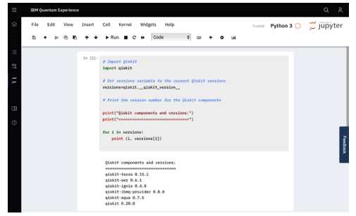
Qiskit” is an open source programming environment that is in continuous flux. Over the course of writing this book, I have passed through many minor and major version updates of the software.

It is generally a good idea to stay updated with the latest version, but with some updates, components of the code might change behavior. It is always a good idea to have a good look at the release notes for each new version. Sometimes changes are introduced that will change the way your code behaves. In those cases, you might want to hold off on upgrading until you have verified that your code still works as expected.

If you are using Anaconda environments, then you can maintain more than one environment at different Qiskit” levels, to have a fallback environment in case an upgraded Qiskit” version breaks your code.
Qiskit” moves fast
The IBM Quantum Experience” Notebook environment always runs the latest version of Qiskit”, and it might be a good idea to test drive your code in that environment before you upgrade your local environment.
You can also subscribe to notification updates, to find out when a new release has been offered:

  1. Log in to IBM Quantum Experience” at https: / /quantum-computing . ibm. com/login.
  2. On the IBM Quantum Experience ${ }^{*}$ dashboard, find your user icon in the upperright corner, click it, and select My account.
  3. On the account page, under Notification settings, set Updates and new feature announcements to $\mathrm{On}$.

物理代写|量子计算代写Quantum computer代考|Comparing a bit and a qubit

So, let’s start with the obvious-or perhaps, not so obvious-notion that most people who read this book know what a bit is.

An intuitive feeling that we have says that a bit is something that is either zero (0) or one (1). By putting many bits together, you can create bytes as well as arbitrary large binary numbers, and with those, build the most amazing computer programs, encode digital images, encrypt your love letters and bank transactions, and more.

In a classical computer, a bit is realized by using low or high voltages over the transistors that make up the logic board, typically something such as $0 \mathrm{~V}$ and $5 \mathrm{~V}$. In a hard drive, the bit might be a region magnetized in a certain way to represent 0 and the other way for 1 , and so on.

In books about quantum computing, the important point to drive home is that a classical bit can only be a 0 or a 1 ; it can never be anything else. In the computer example, you can imagine a box with an input and an output, where the box represents the program that you are running. With a classical computer (and I use the term classical here to indicate a binary computer that is not a quantum computer), the input is a string of bits, the output is another string of bits, and the box is a bunch of bits being manipulated, massaged, and organized to generate that output with some kind of algorithm. An important thing, again, to emphasize is that while in the box, the bits are still bits, always 0 s or $1 \mathrm{~s}$, and nothing else.
A qubit, as we will discover in this chapter, is something quite different. Let’s go explore.

物理代写|量子计算代写Quantum computer代考|Visualizing a qubit in Python

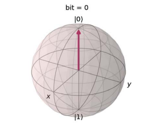
In this recipe, we will use generic Python with NumPy to create a vector and visual representation of a bit and show how it can be in only two states, 0 and 1 . We will also introduce our first, smallish foray into the Qiskit” world by showing how a qubit can not only be in the unique 0 and 1 states but also in a superposition of these states. The way to do this is to take the vector form of the qubit and project it on the so-called Bloch sphere, for which there is a Qiskit” method. Let’s get to work!

In the preceding recipe, we defined our qubits with the help of two complex parameters- $a$ and $b$. This meant that our qubits could take values other than the 0 and 1 of a classical bit. But it is hard to visualize a qubit halfway between 0 and 1 , even if you know $a$ and $b$.

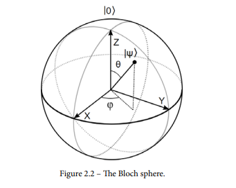
However, with a little mathematical trickery, it turns out that you can also describe a qubit using two angles-theta $(\theta)$ and phi $(\varphi)$-and visualize the qubit on a Bloch sphere. You can think of the $\theta$ and $\varphi$ angles much as the latitude and longitude of the earth. On the Bloch sphere, we can project any possible value that the qubit can take.
The equation for the transformation is as follows:
$$
|\Psi\rangle=\cos \left(\frac{\theta}{2}\right)|0\rangle+\mathrm{e}^{\mathrm{ip}} \sin \left(\frac{\theta}{2}\right)|1\rangle
$$
Here, we use the formula we saw before:
$$
|\psi\rangle=a|0\rangle+b|1\rangle
$$
$a$ and $b$ are, respectively, as follows:
$$
\begin{aligned}
a &=\cos \left(\frac{\theta}{2}\right) \
b &=e^{\mathrm{ip}} \sin \left(\frac{\theta}{2}\right)
\end{aligned}
$$

物理代写|量子计算代写Quantum computer代考|Quantum Computing and Qubits with Python

量子计算代考

物理代写|量子计算代写Quantum computer代考|Keeping your Qiskit® environment up to date

Qiskit”是一个不断变化的开源编程环境。在编写本书的过程中,我经历了软件的许多次要和主要版本更新。

使用最新版本保持更新通常是一个好主意,但随着一些更新,代码的组件可能会改变行为。仔细查看每个新版本的发行说明总是一个好主意。有时会引入更改,从而改变代码的行为方式。在这些情况下,您可能希望推迟升级,直到您确认您的代码仍然按预期工作。

如果您正在使用 Anaconda 环境,那么您可以在不同的 Qiskit” 级别维护多个环境,以拥有一个备用环境,以防升级的 Qiskit” 版本破坏您的代码。
Qiskit” 快速移动
IBM Quantum Experience“笔记本环境始终运行最新版本的 Qiskit”,在升级本地环境之前在该环境中测试驱动代码可能是个好主意。
您还可以订阅通知更新,以了解何时提供新版本:

  1. 登录 IBM Quantum Experience”,网址为 https://quantum-computing。ibm。com/登录。
  2. 关于 IBM Quantum Experience∗仪表板,在右上角找到您的用户图标,单击它,然后选择我的帐户。
  3. 在帐户页面的通知设置下,将更新和新功能公告设置为○n.

物理代写|量子计算代写Quantum computer代考|Comparing a bit and a qubit

所以,让我们从一个明显的(或者也许不是那么明显的)概念开始,大多数读过这本书的人都知道一点是什么。

我们有一种直观的感觉,即位是零 (0) 或一 (1)。通过将许多位放在一起,您可以创建字节以及任意大的二进制数,并使用它们构建最令人惊叹的计算机程序、编码数字图像、加密您的情书和银行交易等等。

在经典计算机中,位是通过在构成逻辑板的晶体管上使用低电压或高电压来实现的,通常例如0 在和5 在. 在硬盘驱动器中,该位可能是以某种方式磁化的区域以表示 0 ,以另一种方式表示 1 ,依此类推。

在有关量子计算的书籍中,重要的一点是经典位只能是 0 或 1 ;它永远不可能是别的东西。在计算机示例中,您可以想象一个带有输入和输出的框,其中框代表您正在运行的程序。对于经典计算机(我在这里使用术语经典来表示不是量子计算机的二进制计算机),输入是一串比特,输出是另一串比特,盒子是一堆比特操纵、按摩和组织以使用某种算法生成该输出。需要再次强调的重要一点是,在盒子中时,位仍然是位,始终为 0 或1 s,仅此而已。
正如我们将在本章中发现的那样,量子比特是完全不同的东西。我们去探索吧。

物理代写|量子计算代写Quantum computer代考|Visualizing a qubit in Python

在这个秘籍中,我们将使用带有 NumPy 的通用 Python 来创建一个位的向量和视觉表示,并展示它如何只处于两种状态,0 和 1。我们还将通过展示量子比特如何不仅可以处于唯一的 0 和 1 状态,而且还可以处于这些状态的叠加状态,来介绍我们对 Qiskit 世界的首次小规模尝试。做到这一点的方法是采用量子比特的向量形式并将其投影到所谓的 Bloch 球体上,对此有一种 Qiskit 方法。让我们开始工作吧!

在前面的秘籍中,我们在两个复杂参数的帮助下定义了我们的量子比特——一个和b. 这意味着我们的量子位可以采用经典位的 0 和 1 以外的值。但是很难想象一个介于 0 和 1 之间的量子比特,即使你知道一个和b.

然而,用一点数学技巧,你也可以用两个角度描述一个量子比特——theta(θ)和 phi(披)- 并在布洛赫球体上可视化量子比特。你可以想到θ和披角度与地球的纬度和经度差不多。在布洛赫球上,我们可以预测量子比特可以取的任何可能值。
变换方程如下:

|Ψ⟩=因⁡(θ2)|0⟩+和一世p罪⁡(θ2)|1⟩
在这里,我们使用之前看到的公式:

|ψ⟩=一个|0⟩+b|1⟩
一个和b分别如下:

一个=因⁡(θ2) b=和一世p罪⁡(θ2)

物理代写|量子计算代写Quantum computer代考| 请认准statistics-lab™

统计代写请认准statistics-lab™. statistics-lab™为您的留学生涯保驾护航。

金融工程代写

金融工程是使用数学技术来解决金融问题。金融工程使用计算机科学、统计学、经济学和应用数学领域的工具和知识来解决当前的金融问题,以及设计新的和创新的金融产品。

非参数统计代写

非参数统计指的是一种统计方法,其中不假设数据来自于由少数参数决定的规定模型;这种模型的例子包括正态分布模型和线性回归模型。

广义线性模型代考

广义线性模型(GLM)归属统计学领域,是一种应用灵活的线性回归模型。该模型允许因变量的偏差分布有除了正态分布之外的其它分布。

术语 广义线性模型(GLM)通常是指给定连续和/或分类预测因素的连续响应变量的常规线性回归模型。它包括多元线性回归,以及方差分析和方差分析(仅含固定效应)。

有限元方法代写

有限元方法(FEM)是一种流行的方法,用于数值解决工程和数学建模中出现的微分方程。典型的问题领域包括结构分析、传热、流体流动、质量运输和电磁势等传统领域。

有限元是一种通用的数值方法,用于解决两个或三个空间变量的偏微分方程(即一些边界值问题)。为了解决一个问题,有限元将一个大系统细分为更小、更简单的部分,称为有限元。这是通过在空间维度上的特定空间离散化来实现的,它是通过构建对象的网格来实现的:用于求解的数值域,它有有限数量的点。边界值问题的有限元方法表述最终导致一个代数方程组。该方法在域上对未知函数进行逼近。[1] 然后将模拟这些有限元的简单方程组合成一个更大的方程系统,以模拟整个问题。然后,有限元通过变化微积分使相关的误差函数最小化来逼近一个解决方案。

tatistics-lab作为专业的留学生服务机构,多年来已为美国、英国、加拿大、澳洲等留学热门地的学生提供专业的学术服务,包括但不限于Essay代写,Assignment代写,Dissertation代写,Report代写,小组作业代写,Proposal代写,Paper代写,Presentation代写,计算机作业代写,论文修改和润色,网课代做,exam代考等等。写作范围涵盖高中,本科,研究生等海外留学全阶段,辐射金融,经济学,会计学,审计学,管理学等全球99%专业科目。写作团队既有专业英语母语作者,也有海外名校硕博留学生,每位写作老师都拥有过硬的语言能力,专业的学科背景和学术写作经验。我们承诺100%原创,100%专业,100%准时,100%满意。

随机分析代写


随机微积分是数学的一个分支,对随机过程进行操作。它允许为随机过程的积分定义一个关于随机过程的一致的积分理论。这个领域是由日本数学家伊藤清在第二次世界大战期间创建并开始的。

时间序列分析代写

随机过程,是依赖于参数的一组随机变量的全体,参数通常是时间。 随机变量是随机现象的数量表现,其时间序列是一组按照时间发生先后顺序进行排列的数据点序列。通常一组时间序列的时间间隔为一恒定值(如1秒,5分钟,12小时,7天,1年),因此时间序列可以作为离散时间数据进行分析处理。研究时间序列数据的意义在于现实中,往往需要研究某个事物其随时间发展变化的规律。这就需要通过研究该事物过去发展的历史记录,以得到其自身发展的规律。

回归分析代写

多元回归分析渐进(Multiple Regression Analysis Asymptotics)属于计量经济学领域,主要是一种数学上的统计分析方法,可以分析复杂情况下各影响因素的数学关系,在自然科学、社会和经济学等多个领域内应用广泛。

MATLAB代写

MATLAB 是一种用于技术计算的高性能语言。它将计算、可视化和编程集成在一个易于使用的环境中,其中问题和解决方案以熟悉的数学符号表示。典型用途包括:数学和计算算法开发建模、仿真和原型制作数据分析、探索和可视化科学和工程图形应用程序开发,包括图形用户界面构建MATLAB 是一个交互式系统,其基本数据元素是一个不需要维度的数组。这使您可以解决许多技术计算问题,尤其是那些具有矩阵和向量公式的问题,而只需用 C 或 Fortran 等标量非交互式语言编写程序所需的时间的一小部分。MATLAB 名称代表矩阵实验室。MATLAB 最初的编写目的是提供对由 LINPACK 和 EISPACK 项目开发的矩阵软件的轻松访问,这两个项目共同代表了矩阵计算软件的最新技术。MATLAB 经过多年的发展,得到了许多用户的投入。在大学环境中,它是数学、工程和科学入门和高级课程的标准教学工具。在工业领域,MATLAB 是高效研究、开发和分析的首选工具。MATLAB 具有一系列称为工具箱的特定于应用程序的解决方案。对于大多数 MATLAB 用户来说非常重要,工具箱允许您学习应用专业技术。工具箱是 MATLAB 函数(M 文件)的综合集合,可扩展 MATLAB 环境以解决特定类别的问题。可用工具箱的领域包括信号处理、控制系统、神经网络、模糊逻辑、小波、仿真等。

R语言代写问卷设计与分析代写
PYTHON代写回归分析与线性模型代写
MATLAB代写方差分析与试验设计代写
STATA代写机器学习/统计学习代写
SPSS代写计量经济学代写
EVIEWS代写时间序列分析代写
EXCEL代写深度学习代写
SQL代写各种数据建模与可视化代写

物理代写|量子计算代写Quantum computer代考|Preparing Your Environment

如果你也在 怎样代写量子计算Quantum computer这个学科遇到相关的难题,请随时右上角联系我们的24/7代写客服。

量子计算机是利用量子物理学的特性来存储数据和进行计算的机器。这对于某些任务来说是非常有利的,它们甚至可以大大超过我们最好的超级计算机。

statistics-lab™ 为您的留学生涯保驾护航 在代写量子计算Quantum computer方面已经树立了自己的口碑, 保证靠谱, 高质且原创的统计Statistics代写服务。我们的专家在代写量子计算Quantum computer代写方面经验极为丰富,各种代写量子计算Quantum computer相关的作业也就用不着说。

我们提供的量子计算Quantum computer及其相关学科的代写,服务范围广, 其中包括但不限于:

  • Statistical Inference 统计推断
  • Statistical Computing 统计计算
  • Advanced Probability Theory 高等概率论
  • Advanced Mathematical Statistics 高等数理统计学
  • (Generalized) Linear Models 广义线性模型
  • Statistical Machine Learning 统计机器学习
  • Longitudinal Data Analysis 纵向数据分析
  • Foundations of Data Science 数据科学基础
物理代写|量子计算代写Quantum computer代考|Preparing Your Environment

物理代写|量子计算代写Quantum computer代考|Technical requirements

The recipes that we will discuss in this chapter can be found here: https://github. com/Packt Publishing/Quantum-Computing-in-Practice-with-Qiskitand-IBM-Quantum-Experience/tree/master/Chapter01.

You can run the recipes in this book in your local Qiskit” environment that you set up as a part of this chapter. You can also run most of them in the Quantum Lab environment of the online IBM Quantum Experience ${ }^{*}$. This is also true for the cl_rl_version.pY recipe in this chapter, which lists the installed version of Qiskit” in the environment in which you run the recipe.

For information about how to download the recipes, see Downloading the code samples.
The local environment in which you choose to install Qiskit” must have Python $3.5$ or higher installed (as of this book’s writing). For detailed information about the most current requirements for Qiskit” installation, see the Qiskit” requirements page at https://qiskit.org/documentation/install. html.
IBM Quantum” recommends using the Anaconda distribution of Python (https:// www . anaconda. com/distribution/), and to use virtual environments to keep your Qiskit” installation isolated from your usual Python environment.

物理代写|量子计算代写Quantum computer代考|Downloading the code samples

The recipes in this book include short, and some not so short, sample programs that will lead you through your first steps in programming quantum computers. You can type in these programs directly from the instructions in the book if you want, but for convenience, you can also grab the sample code directly from the Packt Cookbook GitHub organization.
The Python samples are written for Python $3.5+$ and the Qiskit” extension that you installed in your Python environment. The Python samples all have the extension: $\cdot$ py.

While you can type the recipes directly into your Python environment, or into Jupyter Notebooks on IBM Quantum Experience or on your local Anaconda environment, it is somewhat more efficient to download or use Git to clone the sample code to your local environment. The advantage of cloning is that you can later refresh your local files from the remote repository if any updates are made.

If you do not plan to use Git, but instead to download the recipes as a compressed file, continue on with How to do it.
To use Git to clone the sample code, you must first do the following:

  1. Get a GitHub account. These are free and you can sign up for one at https:// github. com.
  2. Install Git in your local environment. For more information, see https:// git-scm. com/book/en/v2/Getting-Started-Installing-Git.
  3. If you are a user interface person, you might also want to install GitHub Desktop, available here: https: / / desktop.github. com/.

物理代写|量子计算代写Quantum computer代考|Installing your API key and accessing your provider

The main class that you import for this exercise is IBMQ, which is a toolbox for working with the quantum hardware and software that is provided by IBM in the cloud.
In this chapter, we used save. account () to store your account locally. As we go forward, in the recipes where we will access the IBM Quantum” machines, we will use the IBMQ. load_account () and IBMQ.get_provider () classes in your quantum programs to make sure that you have the correct access.
Updating your API key
If for some reason, you need to create a new API token on IBM Quantum Experience” and update your locally saved token, you can use the following command:
There’s more…
In the code that follows in the recipes in this cookbook, we will set a provider variable to hold the provider information for your account by using the following command:
$\Rightarrow$ provider = IBMQ.get provider ()
We can then use the provider information when selecting the IBM Quantum” computer, or backend, to run your quantum programs on. In the following example, we select a quantum computer that is called IBM Q 5 Yorktown (ibmqx2) as our backend. The internal reference for this machine is ibmqx2.

物理代写|量子计算代写Quantum computer代考|Preparing Your Environment

量子计算代考

物理代写|量子计算代写Quantum computer代考|Technical requirements

我们将在本章中讨论的食谱可以在这里找到:https://github。com/Packt Publishing/Quantum-Computing-in-Practice-with-Qiskitand-IBM-Quantum-Experience/tree/master/Chapter01。

您可以在作为本章一部分设置的本地 Qiskit 环境中运行本书中的食谱。您还可以在在线 IBM Quantum Experience 的 Quantum Lab 环境中运行它们中的大部分∗. 本章中的 cl_rl_version.pY 配方也是如此,它列出了运行该配方的环境中已安装的 Qiskit 版本。

有关如何下载配方的信息,请参阅下载代码示例。
您选择安装 Qiskit 的本地环境”必须有 Python3.5安装或更高版本(截至本书撰写时)。有关 Qiskit” 安装最新要求的详细信息,请参阅 https://qiskit.org/documentation/install 上的 Qiskit” 要求页面。html。
IBM Quantum”建议使用 Python 的 Anaconda 发行版 (https://www.anaconda.com/distribution/),并使用虚拟环境使您的 Qiskit”安装与您通常的 Python 环境隔离。

物理代写|量子计算代写Quantum computer代考|Downloading the code samples

本书中的秘籍包括一些简短的示例程序,其中一些示例程序将引导您完成量子计算机编程的第一步。如果需要,您可以直接从书中的说明中输入这些程序,但为方便起见,您也可以直接从 Packt Cookbook GitHub 组织中获取示例代码。
Python 示例是为 Python 编写的3.5+以及您在 Python 环境中安装的 Qiskit”扩展。Python 示例都具有扩展名:⋅py。

虽然您可以将配方直接输入到 Python 环境中,或者输入到 IBM Quantum Experience 上的 Jupyter Notebooks 或本地 Anaconda 环境中,但下载或使用 Git 将示例代码克隆到本地环境会更有效。克隆的优点是,如果进行了任何更新,您可以稍后从远程存储库刷新本地文件。

如果您不打算使用 Git,而是将配方下载为压缩文件,请继续阅读如何操作。
要使用 Git 克隆示例代码,您必须首先执行以下操作:

  1. 获取一个 GitHub 帐户。这些是免费的,您可以在 https://github 上注册一个。com。
  2. 在本地环境中安装 Git。有关详细信息,请参阅 https://git-scm。com/book/en/v2/Getting-Started-Installing-Git。
  3. 如果您是用户界面人,您可能还想安装 GitHub Desktop,可在此处获得:https://desktop.github。com/.

物理代写|量子计算代写Quantum computer代考|Installing your API key and accessing your provider

您为本练习导入的主要类是 IBMQ,它是一个工具箱,用于处理 IBM 在云中提供的量子硬件和软件。
在本章中,我们使用了 save。account() 将您的帐户存储在本地。随着我们前进,在我们将访问 IBM Quantum 机器的配方中,我们将使用 IBMQ。load_account () 和 IBMQ.get_provider () 类,以确保您具有正确的访问权限。
更新您的 API 密钥
如果出于某种原因,您需要在 IBM Quantum Experience 上创建一个新的 API 令牌并更新您本地保存的令牌,您可以使用以下命令:
还有更多……
在本食谱后面的代码中,我们将使用以下命令设置一个提供者变量来保存您帐户的提供者信息:
⇒provider = IBMQ.get provider ()
然后,我们可以在选择 IBM Quantum 计算机或后端时使用提供者信息来运行您的量子程序。在以下示例中,我们选择名为 IBM Q 5 Yorktown (ibmqx2) 的量子计算机作为我们的后端。这台机器的内部参考是 ibmqx2。

物理代写|量子计算代写Quantum computer代考| 请认准statistics-lab™

统计代写请认准statistics-lab™. statistics-lab™为您的留学生涯保驾护航。

金融工程代写

金融工程是使用数学技术来解决金融问题。金融工程使用计算机科学、统计学、经济学和应用数学领域的工具和知识来解决当前的金融问题,以及设计新的和创新的金融产品。

非参数统计代写

非参数统计指的是一种统计方法,其中不假设数据来自于由少数参数决定的规定模型;这种模型的例子包括正态分布模型和线性回归模型。

广义线性模型代考

广义线性模型(GLM)归属统计学领域,是一种应用灵活的线性回归模型。该模型允许因变量的偏差分布有除了正态分布之外的其它分布。

术语 广义线性模型(GLM)通常是指给定连续和/或分类预测因素的连续响应变量的常规线性回归模型。它包括多元线性回归,以及方差分析和方差分析(仅含固定效应)。

有限元方法代写

有限元方法(FEM)是一种流行的方法,用于数值解决工程和数学建模中出现的微分方程。典型的问题领域包括结构分析、传热、流体流动、质量运输和电磁势等传统领域。

有限元是一种通用的数值方法,用于解决两个或三个空间变量的偏微分方程(即一些边界值问题)。为了解决一个问题,有限元将一个大系统细分为更小、更简单的部分,称为有限元。这是通过在空间维度上的特定空间离散化来实现的,它是通过构建对象的网格来实现的:用于求解的数值域,它有有限数量的点。边界值问题的有限元方法表述最终导致一个代数方程组。该方法在域上对未知函数进行逼近。[1] 然后将模拟这些有限元的简单方程组合成一个更大的方程系统,以模拟整个问题。然后,有限元通过变化微积分使相关的误差函数最小化来逼近一个解决方案。

tatistics-lab作为专业的留学生服务机构,多年来已为美国、英国、加拿大、澳洲等留学热门地的学生提供专业的学术服务,包括但不限于Essay代写,Assignment代写,Dissertation代写,Report代写,小组作业代写,Proposal代写,Paper代写,Presentation代写,计算机作业代写,论文修改和润色,网课代做,exam代考等等。写作范围涵盖高中,本科,研究生等海外留学全阶段,辐射金融,经济学,会计学,审计学,管理学等全球99%专业科目。写作团队既有专业英语母语作者,也有海外名校硕博留学生,每位写作老师都拥有过硬的语言能力,专业的学科背景和学术写作经验。我们承诺100%原创,100%专业,100%准时,100%满意。

随机分析代写


随机微积分是数学的一个分支,对随机过程进行操作。它允许为随机过程的积分定义一个关于随机过程的一致的积分理论。这个领域是由日本数学家伊藤清在第二次世界大战期间创建并开始的。

时间序列分析代写

随机过程,是依赖于参数的一组随机变量的全体,参数通常是时间。 随机变量是随机现象的数量表现,其时间序列是一组按照时间发生先后顺序进行排列的数据点序列。通常一组时间序列的时间间隔为一恒定值(如1秒,5分钟,12小时,7天,1年),因此时间序列可以作为离散时间数据进行分析处理。研究时间序列数据的意义在于现实中,往往需要研究某个事物其随时间发展变化的规律。这就需要通过研究该事物过去发展的历史记录,以得到其自身发展的规律。

回归分析代写

多元回归分析渐进(Multiple Regression Analysis Asymptotics)属于计量经济学领域,主要是一种数学上的统计分析方法,可以分析复杂情况下各影响因素的数学关系,在自然科学、社会和经济学等多个领域内应用广泛。

MATLAB代写

MATLAB 是一种用于技术计算的高性能语言。它将计算、可视化和编程集成在一个易于使用的环境中,其中问题和解决方案以熟悉的数学符号表示。典型用途包括:数学和计算算法开发建模、仿真和原型制作数据分析、探索和可视化科学和工程图形应用程序开发,包括图形用户界面构建MATLAB 是一个交互式系统,其基本数据元素是一个不需要维度的数组。这使您可以解决许多技术计算问题,尤其是那些具有矩阵和向量公式的问题,而只需用 C 或 Fortran 等标量非交互式语言编写程序所需的时间的一小部分。MATLAB 名称代表矩阵实验室。MATLAB 最初的编写目的是提供对由 LINPACK 和 EISPACK 项目开发的矩阵软件的轻松访问,这两个项目共同代表了矩阵计算软件的最新技术。MATLAB 经过多年的发展,得到了许多用户的投入。在大学环境中,它是数学、工程和科学入门和高级课程的标准教学工具。在工业领域,MATLAB 是高效研究、开发和分析的首选工具。MATLAB 具有一系列称为工具箱的特定于应用程序的解决方案。对于大多数 MATLAB 用户来说非常重要,工具箱允许您学习应用专业技术。工具箱是 MATLAB 函数(M 文件)的综合集合,可扩展 MATLAB 环境以解决特定类别的问题。可用工具箱的领域包括信号处理、控制系统、神经网络、模糊逻辑、小波、仿真等。

R语言代写问卷设计与分析代写
PYTHON代写回归分析与线性模型代写
MATLAB代写方差分析与试验设计代写
STATA代写机器学习/统计学习代写
SPSS代写计量经济学代写
EVIEWS代写时间序列分析代写
EXCEL代写深度学习代写
SQL代写各种数据建模与可视化代写

计算机代写|量子计算代写Quantum computing代考|Novel Reconstructability Analysis Circuits

如果你也在 怎样代写量子计算Quantum computing这个学科遇到相关的难题,请随时右上角联系我们的24/7代写客服。

量子计算是一种利用量子态的集体特性,如叠加、干涉和纠缠,来进行计算的计算方式。

statistics-lab™ 为您的留学生涯保驾护航 在代写量子计算Quantum computing方面已经树立了自己的口碑, 保证靠谱, 高质且原创的统计Statistics代写服务。我们的专家在代写量子计算Quantum computing代写方面经验极为丰富,各种代写量子计算Quantum computing相关的作业也就用不着说。

我们提供的量子计算Quantum computing及其相关学科的代写,服务范围广, 其中包括但不限于:

  • Statistical Inference 统计推断
  • Statistical Computing 统计计算
  • Advanced Probability Theory 高等概率论
  • Advanced Mathematical Statistics 高等数理统计学
  • (Generalized) Linear Models 广义线性模型
  • Statistical Machine Learning 统计机器学习
  • Longitudinal Data Analysis 纵向数据分析
  • Foundations of Data Science 数据科学基础
计算机代写|量子计算代写Quantum computing代考|Novel Reconstructability Analysis Circuits

计算机代写|量子计算代写Quantum computing代考|Reversible Realizations

This Chapt. will introduce another new type of reversible structures called Reversible Modified Reconstructability Analysis (RMRA). Reconstructability Analysis (RA) is an important decomposition technique that is used widely in system science area to decompose qualitative data $[133,134,135,138,273,275]$. This kind of decomposition is commonly used in the decomposition of data obtained in the social and system science fields, and overlaps with other decomposition techniques used in the social sciences as well like the Log-Linear (LL) decomposition method [138]. RA decomposition aims at the simplest decomposition of qualitative data using Lattice-Of-Structure (LOS) (cf. Fig. 7.1) as representation (generation) and contingency tables (for probabilistic data) for evaluation (minimization of error).

In lossless decomposition, the aim is to obtain the simplest decomposed model from data (saturated model) without the loss of any information (i.e., error $=0$ ). In lossy decomposition, the aim is to obtain the simplest decomposed model from data (saturated model) with an acceptable amount of error. RA data is typically either a set-theoretic relation [271,272] (or mapping) or it is a probability (or frequency) distribution. The former case is the domain of set-theoretic RA or more precisely crisp possibilistic RA. The latter is the domain of information-theoretic RA, or more precisely probabilistic RA $[133,134,135,138,274]$. The RA framework can apply to other types of data (e.g., fuzzy data) via generalized information theory $[135,223]$. In this work, we are concerned only with crisp possibilistic RA.

计算机代写|量子计算代写Quantum computing代考|New Type of Reconstructability Analysis

This Sect. introduces an innovation in set-theoretic RA, which we call “modified” RA (or MRA) as opposed to the conventional settheoretic RA (or CRA). This innovation will be illustrated by Examples $7.1$ and 7.2. The main idea of MRA stems from the following fact: While the conventional RA (CRA) decomposes on the set of all functional values of the corresponding function, the modified RA (MRA) decomposes on the set of minimum functional values from which the function can be totally reconstructed. In general, the procedure for the lossless MRA decomposition follows the following steps:
(1) Using the lattice-of-relations, decompose for one value only of the Boolean function into the simplest error-free decomposed structure:
(1a) Remove one relation between variables from the previous level.
(1b) Add the embedded relation(s) between variables, in the current level, if they are not already present in the new model.
(2) As a result of step 1, one obtains MRA decomposition for value “1” of the Boolean function (denoted as 1-MRA decomposition), and MRA decomposition for value ” 0 ” of the Boolean function (denoted as 0-MRA decomposition). Select the simplest model from

the resulting 1-MRA decomposition and the 0-MRA decomposition, respectively.
(3) In the resulting simplest decomposed data model from step 2, generate the corresponding sub-functional values for each interaction (relation) between the variables that exist in the decomposed model.
(4) Generate the total functional values using the intersection between all possible sub-functional values for 1-MRA, and the union between all possible sub-functional values for 0-MRA.
Example 7.1. Figure $7.2$ illustrates decomposed structures using both CRA and MRA decompositions, respectively for the logic function: $F=x_{1} x_{2}+x_{1} x_{3}$.

计算机代写|量子计算代写Quantum computing代考|Multiple-Valued MRA

Real-life data are in general many-valued. Consequently, if MRA can decompose relations between many-valued variables it can have practical applications in machine learning (ML) and data mining (DM). Many-valued MRA is made up of two main steps which are common to two equivalent (intersection-based and union-based) algorithms as follows:
(1) partition the many-valued truth table into sub-tables, each contain only single functional value.
(2) Perform CRA on all sub-tables. Figure $7.5$ illustrates the general pre-processing procedure for the two many-valued MRA algorithms, which will be explained in more detail below.

For an “n”-valued completely specified function one needs (n-1) values to define the function (i.e., to be able to retrieve the completely specified function without any loss of information). We thus do all $\mathrm{n}$ decompositions and use for our MRA model the (n-1) simplest of these. Figure $7.5$ illustrates the general flow diagram of the multiple-valued MRA decomposition using the pre-processing steps that are common to both of the intersection-based and unionbased algorithms.

For example, using the lattice-of-structures, decompose the 3valued function for each individual value. One then obtains the simplest lossless MRA decomposition for value “0” of the function (denoted as the 0-MRA decomposition), for value “1” (1-MRA decomposition), and for value “2” (2-MRA decomposition). By selecting the simplest two models from these 0-MRA, 1-MRA, and 2-MRA decompositions, one can generate the complete function.

计算机代写|量子计算代写Quantum computing代考|Novel Reconstructability Analysis Circuits

量子计算代考

计算机代写|量子计算代写Quantum computing代考|Reversible Realizations

这章。将介绍另一种新型可逆结构,称为可逆修正可重构性分析 (RMRA)。可重构性分析(RA)是一种重要的分解技术,在系统科学领域广泛用于分解定性数据[133,134,135,138,273,275]. 这种分解通常用于社会和系统科学领域获得的数据的分解,并且与社会科学中使用的其他分解技术以及对数线性(LL)分解方法重叠[138]。RA 分解旨在使用 Lattice-Of-Structure (LOS)(参见图 7.1)作为表示(生成)和用于评估(最小化误差)的列联表(用于概率数据)对定性数据进行最简单的分解。

在无损分解中,目标是从数据中得到最简单的分解模型(饱和模型)而不损失任何信息(即误差=0)。在有损分解中,目标是从数据(饱和模型)中获得最简单的分解模型,并具有可接受的误差量。RA 数据通常是集合论关系 [271,272](或映射),或者是概率(或频率)分布。前一种情况是集合论 RA 或更准确地说是清晰的可能 RA 的域。后者是信息论 RA 的领域,或更准确地说是概率 RA[133,134,135,138,274]. RA 框架可以通过广义信息论应用于其他类型的数据(例如,模糊数据)[135,223]. 在这项工作中,我们只关心清晰的可能 RA。

计算机代写|量子计算代写Quantum computing代考|New Type of Reconstructability Analysis

本门派。引入了集合论 RA 的创新,我们将其称为“修改的”RA(或 MRA),而不是传统的集合论 RA(或 CRA)。这种创新将通过示例来说明7.1和 7.2。MRA 的主要思想源于以下事实:传统 RA (CRA) 分解在相应函数的所有函数值的集合上,而改进的 RA (MRA) 分解在函数可以从中得到的最小函数值的集合上。被完全重建。一般来说,无损 MRA 分解的过程遵循以下步骤:
(1) 使用关系格,仅将布尔函数的一个值分解为最简单的无错误分解结构:
(1a) 删除一个关系上一级的变量之间。
(1b) 在当前级别添加变量之间的嵌入关系,如果它们尚未出现在新模型中。
(2) 作为步骤 1 的结果,得到布尔函数值“1”的 MRA 分解(记作 1-MRA 分解),以及布尔函数值“0”的 MRA 分解(记作 0-MRA分解)。选择最简单的模型

分别得到 1-MRA 分解和 0-MRA 分解。
(3) 在从步骤 2 得到的最简单的分解数据模型中,为分解模型中存在的变量之间的每个交互(关系)生成相应的子功能值。
(4) 使用 1-MRA 的所有可能子功能值之间的交集和 0-MRA 的所有可能子功能值之间的并集来生成总功能值。
例 7.1。数字7.2分别使用 CRA 和 MRA 分解来说明逻辑函数的分解结构:F=X1X2+X1X3.

计算机代写|量子计算代写Quantum computing代考|Multiple-Valued MRA

现实生活中的数据通常是多值的。因此,如果 MRA 可以分解多值变量之间的关系,它就可以在机器学习 (ML) 和数据挖掘 (DM) 中具有实际应用。多值 MRA 由两个等价(基于交集和基于联合)算法共有的两个主要步骤组成,如下所示:
(1)将多值真值表划分为子表,每个子表仅包含单个功能价值。
(2)对所有子表进行CRA。数字7.5图 1 说明了两种多值 MRA 算法的一般预处理过程,这将在下面更详细地解释。

对于“n”值的完全指定函数,需要 (n-1) 个值来定义函数(即,能够检索完全指定的函数而不会丢失任何信息)。我们因此做所有n分解并为我们的 MRA 模型使用 (n-1) 个最简单的。数字7.5说明了多值 MRA 分解的一般流程图,使用基于交集和基于联合的算法都通用的预处理步骤。

例如,使用 lattice-of-structures,分解每个单独值的 3 值函数。然后为函数的值“0”(表示为 0-MRA 分解)、值“1”(1-MRA 分解)和值“2”(2-MRA 分解)获得最简单的无损 MRA 分解. 通过从这些 0-MRA、1-MRA 和 2-MRA 分解中选择最简单的两个模型,可以生成完整的函数。

计算机代写|量子计算代写Quantum computing代考 请认准statistics-lab™

统计代写请认准statistics-lab™. statistics-lab™为您的留学生涯保驾护航。

金融工程代写

金融工程是使用数学技术来解决金融问题。金融工程使用计算机科学、统计学、经济学和应用数学领域的工具和知识来解决当前的金融问题,以及设计新的和创新的金融产品。

非参数统计代写

非参数统计指的是一种统计方法,其中不假设数据来自于由少数参数决定的规定模型;这种模型的例子包括正态分布模型和线性回归模型。

广义线性模型代考

广义线性模型(GLM)归属统计学领域,是一种应用灵活的线性回归模型。该模型允许因变量的偏差分布有除了正态分布之外的其它分布。

术语 广义线性模型(GLM)通常是指给定连续和/或分类预测因素的连续响应变量的常规线性回归模型。它包括多元线性回归,以及方差分析和方差分析(仅含固定效应)。

有限元方法代写

有限元方法(FEM)是一种流行的方法,用于数值解决工程和数学建模中出现的微分方程。典型的问题领域包括结构分析、传热、流体流动、质量运输和电磁势等传统领域。

有限元是一种通用的数值方法,用于解决两个或三个空间变量的偏微分方程(即一些边界值问题)。为了解决一个问题,有限元将一个大系统细分为更小、更简单的部分,称为有限元。这是通过在空间维度上的特定空间离散化来实现的,它是通过构建对象的网格来实现的:用于求解的数值域,它有有限数量的点。边界值问题的有限元方法表述最终导致一个代数方程组。该方法在域上对未知函数进行逼近。[1] 然后将模拟这些有限元的简单方程组合成一个更大的方程系统,以模拟整个问题。然后,有限元通过变化微积分使相关的误差函数最小化来逼近一个解决方案。

tatistics-lab作为专业的留学生服务机构,多年来已为美国、英国、加拿大、澳洲等留学热门地的学生提供专业的学术服务,包括但不限于Essay代写,Assignment代写,Dissertation代写,Report代写,小组作业代写,Proposal代写,Paper代写,Presentation代写,计算机作业代写,论文修改和润色,网课代做,exam代考等等。写作范围涵盖高中,本科,研究生等海外留学全阶段,辐射金融,经济学,会计学,审计学,管理学等全球99%专业科目。写作团队既有专业英语母语作者,也有海外名校硕博留学生,每位写作老师都拥有过硬的语言能力,专业的学科背景和学术写作经验。我们承诺100%原创,100%专业,100%准时,100%满意。

随机分析代写


随机微积分是数学的一个分支,对随机过程进行操作。它允许为随机过程的积分定义一个关于随机过程的一致的积分理论。这个领域是由日本数学家伊藤清在第二次世界大战期间创建并开始的。

时间序列分析代写

随机过程,是依赖于参数的一组随机变量的全体,参数通常是时间。 随机变量是随机现象的数量表现,其时间序列是一组按照时间发生先后顺序进行排列的数据点序列。通常一组时间序列的时间间隔为一恒定值(如1秒,5分钟,12小时,7天,1年),因此时间序列可以作为离散时间数据进行分析处理。研究时间序列数据的意义在于现实中,往往需要研究某个事物其随时间发展变化的规律。这就需要通过研究该事物过去发展的历史记录,以得到其自身发展的规律。

回归分析代写

多元回归分析渐进(Multiple Regression Analysis Asymptotics)属于计量经济学领域,主要是一种数学上的统计分析方法,可以分析复杂情况下各影响因素的数学关系,在自然科学、社会和经济学等多个领域内应用广泛。

MATLAB代写

MATLAB 是一种用于技术计算的高性能语言。它将计算、可视化和编程集成在一个易于使用的环境中,其中问题和解决方案以熟悉的数学符号表示。典型用途包括:数学和计算算法开发建模、仿真和原型制作数据分析、探索和可视化科学和工程图形应用程序开发,包括图形用户界面构建MATLAB 是一个交互式系统,其基本数据元素是一个不需要维度的数组。这使您可以解决许多技术计算问题,尤其是那些具有矩阵和向量公式的问题,而只需用 C 或 Fortran 等标量非交互式语言编写程序所需的时间的一小部分。MATLAB 名称代表矩阵实验室。MATLAB 最初的编写目的是提供对由 LINPACK 和 EISPACK 项目开发的矩阵软件的轻松访问,这两个项目共同代表了矩阵计算软件的最新技术。MATLAB 经过多年的发展,得到了许多用户的投入。在大学环境中,它是数学、工程和科学入门和高级课程的标准教学工具。在工业领域,MATLAB 是高效研究、开发和分析的首选工具。MATLAB 具有一系列称为工具箱的特定于应用程序的解决方案。对于大多数 MATLAB 用户来说非常重要,工具箱允许您学习应用专业技术。工具箱是 MATLAB 函数(M 文件)的综合集合,可扩展 MATLAB 环境以解决特定类别的问题。可用工具箱的领域包括信号处理、控制系统、神经网络、模糊逻辑、小波、仿真等。

R语言代写问卷设计与分析代写
PYTHON代写回归分析与线性模型代写
MATLAB代写方差分析与试验设计代写
STATA代写机器学习/统计学习代写
SPSS代写计量经济学代写
EVIEWS代写时间序列分析代写
EXCEL代写深度学习代写
SQL代写各种数据建模与可视化代写

计算机代写|量子计算代写Quantum computing代考|Fundamentals and New Results

如果你也在 怎样代写量子计算Quantum computing这个学科遇到相关的难题,请随时右上角联系我们的24/7代写客服。

量子计算是一种利用量子态的集体特性,如叠加、干涉和纠缠,来进行计算的计算方式。

statistics-lab™ 为您的留学生涯保驾护航 在代写量子计算Quantum computing方面已经树立了自己的口碑, 保证靠谱, 高质且原创的统计Statistics代写服务。我们的专家在代写量子计算Quantum computing代写方面经验极为丰富,各种代写量子计算Quantum computing相关的作业也就用不着说。

我们提供的量子计算Quantum computing及其相关学科的代写,服务范围广, 其中包括但不限于:

  • Statistical Inference 统计推断
  • Statistical Computing 统计计算
  • Advanced Probability Theory 高等概率论
  • Advanced Mathematical Statistics 高等数理统计学
  • (Generalized) Linear Models 广义线性模型
  • Statistical Machine Learning 统计机器学习
  • Longitudinal Data Analysis 纵向数据分析
  • Foundations of Data Science 数据科学基础
计算机代写|量子计算代写Quantum computing代考|Fundamentals and New Results

计算机代写|量子计算代写Quantum computing代考|Fundamentals and New Results

Due to the anticipated failure of Moore’s law around the year 2020 , quantum computing will hopefully play an increasingly crucial role in building more compact and less power consuming computers $[93,107,167,248,253]$. Due to this fact, and because all quantum computer gates (i.e., building blocks; primitives) must be reversible $[37,38,39,73,74,75,95,97,139,150,167,203,245,246]$ reversibility in computing will have increasing importance in the future design of regular, compact, and universal structures and machines (systems). $(\mathrm{n}, \mathrm{k})$ reversible circuits are circuits that have (n) inputs and (k) outputs and are one-to-one mappings between vectors of inputs and outputs, thus the vector of input states (values) can be always uniquely reconstructed from the vector of output states (values). $(k, k)$ reversible circuits are circuits that have the same number of inputs $(\mathrm{k})$ and outputs $(\mathrm{k})$ and are one-to-one mappings between vectors of inputs and outputs, thus the vector of input states (values) can be always uniquely reconstructed from the vector of output states (values). Conservative circuits $[98,210,211,212]$ are circuits that have the same number of values in inputs and outputs (e.g., the same number of ones in inputs and outputs for binary, the same number of ones and twos in inputs and outputs for ternary, etc). Conservativeness exists naturally in physical laws where no energy is created or destroyed.

As was proven in $[37,139]$ it is a necessary but not sufficient condition for not dissipating power in any physical circuit that all system circuits must be built using fully reversible logical components. An important argument for power-free computation in a computer that “pushes information around” using reversible logic is given in [139], using the model of a particle in a bistable potential well, as follows.

计算机代写|量子计算代写Quantum computing代考|Fundamental Reversible Logic Primitives and Circuits

Reversible circuits which are hierarchically composed of reversible primitives have two types of outputs in general: (1) functionality outputs, and (2) outputs that are needed only to achieve reversibility which are called “garbage” [98]. Many reversible gates have been proposed as building blocks for reversible (and consequently quantum) computing. Figure $5.4$ shows some of the binary $(\mathrm{k}, \mathrm{k})$ reversible gates that are commonly used in the synthesis of reversible logic circuits $[6,14,95,126,127,128,129]$. It is noted from Fig. $5.4$ that while Wire (Buffer), Not, and Swap gates are naturally reversible, others are not, and thus “garbage” has to be added.Multiple-valued counterparts of similar reversible primitives and some of their applications were introduced in $[6,11,14,190,191,192,193]$. Figure $5.5$ illustrates the multiple-valued gate from [191]. More multiple-valued gates and the systematic methodology for their creation and classification will be introduced in Sect. 5.4.

Although most of available literature on reversible computing presents gates that are $(k, k)$ reversible, other literature has reported the conceptual need for $(\mathrm{n}, \mathrm{k})$ reversible primitives in general. The need for $(n, k)$ reversible primitives stems from the fact that the logical model must fit the physical reality of computing, and not to be disjoint from the physical laws of computing as it was in the previous abstract mathematical logics before reversible (and thus quantum) computing. For instance, the Interaction gate $[62,63,64,222]$ has been reported to be of a good fit to reversible computing in optics. Figure $5.6$ illustrates some of the $(\mathrm{n}, \mathrm{k})$ reversible gates. (It is important to note that here fan-out and feedback are not allowed in reversible computing applications using either $(\mathrm{k}, \mathrm{k})$ reversible gates or $(\mathrm{n}, \mathrm{k})$ reversible gates.)

Fredkin gate [98] is one of the most basic building blocks in reversible and quantum computing. Many propositions have been proposed to realize the Fredkin gate in various technologies: Optical, Electrical, Mechanical (nano-technology), and Quantum. The Fredkin gate belongs to a group of gates that each represents a fundamental family of logic gates in reversible computing. These families of reversible gates are Fredkin-like, Toffoli-like, and Feynman-like gates. It will be shown in Sect. $5.4$ how to formally generalize the Fredkin gate to any multiple-valued logic radix.

计算机代写|量子计算代写Quantum computing代考|Combinational Reversible Circuits

Reversible circuits can be synthesized using careful design methodologies where one utilizes the outputs from a previous stage as inputs to the next stage. Various reversible circuits have been synthesized using this methodology [8,200]. This Sect. introduces some of these circuits. Figure $5.15$ illustrates the creation of all of the 16 possible binary logic functions of two variables (cf. Fig. G.3 in Appendix G) using certain reversible logic primitives.

Note that such constructions are not unique, and thus the optimization criteria should be (1) minimum size and (2) have mimimum garbage used in the synthesis. Figure $5.16$ illustrates the synthesis of half-adder and full-adder using Feynman (ControlledNOT: CN) and Toffoli (Controlled-Controlled-NOT: CCN) gates.

As shifters are important in combinational and sequential logic synthesis, it is important to produce a reversible logic shifter. Figure $5.18$ illustrates a novel reversible Barrel shifter design from [8]. Figure $5.18$ represents one possible design of concurrent shift-left and shift-right reversible Barrel shifter, which shows a fundamental concept in the design of reversible logic circuits: the idea of the use of reversibility to perform multiple operations using the same design while retaining reversibility [8].

Note that by controlling the value of the variable in the first level, the Barrel shifter operates in the shift-left mode by setting the value of variable $X$ in the first level to value “0” and collecting the shifted-left outputs from the locations that are marked by $(X)$ at the outputs of Fredkin gates, or the shift-right mode by setting the value of variable $X$ in the first level to value ” 1 ” and collecting the shiftedright outputs from the locations that are marked by ( $+)$ at the outputs of Fredkin gates, respectively. The first level of the reversible Barrel shifter will shift the inputs by one location, the second level will shift the inputs by two locations, the third level will shift the inputs by three locations, and the fourth level will shift the inputs by four locations (i.e., full cycle or rotation).

Figure $5.19$ illustrates the use of MIN/MAX gate, which is synthesized from Picton gate, to realize a multiple-valued Sorter [8]. By following the paths, from the inputs to the outputs, one will obtain the sorted values of the inputs at the outputs.

计算机代写|量子计算代写Quantum computing代考|Fundamentals and New Results

量子计算代考

计算机代写|量子计算代写Quantum computing代考|Fundamentals and New Results

由于摩尔定律在 2020 年左右的预期失效,量子计算有望在构建更紧凑、功耗更低的计算机方面发挥越来越重要的作用[93,107,167,248,253]. 由于这个事实,并且因为所有量子计算机门(即构建块;基元)必须是可逆的[37,38,39,73,74,75,95,97,139,150,167,203,245,246]计算中的可逆性将在未来设计规则、紧凑和通用的结构和机器(系统)中变得越来越重要。(n,ķ)可逆电路是具有(n)个输入和(k)个输出的电路,并且是输入和输出向量之间的一对一映射,因此输入状态(值)向量总是可以从输出状态向量唯一地重建(值)。(ķ,ķ)可逆电路是具有相同输入数的电路(ķ)和输出(ķ)并且是输入和输出向量之间的一对一映射,因此输入状态(值)向量总是可以从输出状态(值)向量中唯一地重建。保守电路[98,210,211,212]是在输入和输出中具有相同数量值的电路(例如,对于二进制而言,输入和输出中具有相同数量的 1,对于三进制而言,输入和输出中具有相同数量的 1 和 2 等)。保守性自然存在于物理定律中,不会产生或破坏能量。

正如在[37,139]必须使用完全可逆的逻辑组件来构建所有系统电路,这是在任何物理电路中不耗散功率的必要但非充分条件。[139] 中给出了计算机中使用可逆逻辑“推动信息”的无功率计算的重要论据,使用双稳态势阱中的粒子模型,如下所示。

计算机代写|量子计算代写Quantum computing代考|Fundamental Reversible Logic Primitives and Circuits

由可逆原语分层组成的可逆电路通常具有两种类型的输出:(1)功能输出,和(2)仅用于实现可逆性的输出,称为“垃圾”[98]。许多可逆门已被提议作为可逆(以及因此量子)计算的构建块。数字5.4显示一些二进制文件(ķ,ķ)可逆逻辑电路合成中常用的可逆门[6,14,95,126,127,128,129]. 从图中可以看出。5.4虽然 Wire (Buffer)、Not 和 Swap 门是自然可逆的,但其他门不是,因此必须添加“垃圾”。类似可逆原语的多值对应物及其一些应用在[6,11,14,190,191,192,193]. 数字5.5说明了[191]中的多值门。更多的多值门及其创建和分类的系统方法将在第 3 节中介绍。5.4.

尽管大多数关于可逆计算的可用文献都提出了(ķ,ķ)可逆,其他文献报道了概念上的需要(n,ķ)一般的可逆基元。需要(n,ķ)可逆原语源于这样一个事实,即逻辑模型必须适合计算的物理现实,并且不能像在可逆(以及量子)计算之前的先前抽象数学逻辑中那样与计算的物理定律脱节。例如,交互门[62,63,64,222]据报道,它非常适合光学中的可逆计算。数字5.6说明了一些(n,ķ)可逆门。(重要的是要注意,在可逆计算应用程序中不允许使用扇出和反馈(ķ,ķ)可逆门或(n,ķ)可逆门。)

Fredkin Gate [98] 是可逆和量子计算中最基本的构建模块之一。已经提出了许多命题来在各种技术中实现 Fredkin 门:光学、电气、机械(纳米技术)和量子。Fredkin 门属于一组门,每个门都代表可逆计算中的一个基本逻辑门家族。这些可逆门家族是 Fredkin-like、Toffoli-like 和 Feynman-like gates。它将在Sect中显示。5.4如何将 Fredkin 门正式推广到任何多值逻辑基数。

计算机代写|量子计算代写Quantum computing代考|Combinational Reversible Circuits

可以使用仔细的设计方法合成可逆电路,其中将前一级的输出用作下一级的输入。已经使用这种方法合成了各种可逆电路 [8,200]。本门派。介绍了其中一些电路。数字5.15说明了使用某些可逆逻辑原语创建两个变量的所有 16 种可能的二进制逻辑函数(参见附录 G 中的图 G.3)。

请注意,此类构造不是唯一的,因此优化标准应为 (1) 最小尺寸和 (2) 在合成中使用的垃圾最少。数字5.16说明了使用 Feynman (ControlledNOT: CN) 和 Toffoli (Controlled-Controlled-NOT: CCN) 门合成半加器和全加器。

由于移位器在组合逻辑和时序逻辑综合中很重要,因此产生可逆逻辑移位器很重要。数字5.18说明了来自 [8] 的一种新颖的可逆桶形移位器设计。数字5.18代表了一种可能的并发左移和右移可逆桶式移位器设计,它展示了可逆逻辑电路设计中的一个基本概念:使用可逆性使用相同设计执行多个操作同时保持可逆性的想法 [8 ]。

请注意,通过控制第一级中变量的值,桶移位器通过设置变量的值以左移模式运行X在第一级中设置为“0”并从标记的位置收集左移输出(X)在 Fredkin 门的输出端,或通过设置变量的值来右移模式X在第一级为“1”赋值,并从标记为 (+)分别在 Fredkin 门的输出端。可逆桶形移位器的第一级将输入移动一个位置,第二级将输入移动两个位置,第三级将输入移动三个位置,第四级将输入移动四个位置(即,全周期或旋转)。

数字5.19说明了使用由皮克顿门合成的 MIN/MAX 门来实现多值排序器 [8]。通过遵循从输入到输出的路径,可以在输出处获得输入的排序值。

计算机代写|量子计算代写Quantum computing代考 请认准statistics-lab™

统计代写请认准statistics-lab™. statistics-lab™为您的留学生涯保驾护航。

金融工程代写

金融工程是使用数学技术来解决金融问题。金融工程使用计算机科学、统计学、经济学和应用数学领域的工具和知识来解决当前的金融问题,以及设计新的和创新的金融产品。

非参数统计代写

非参数统计指的是一种统计方法,其中不假设数据来自于由少数参数决定的规定模型;这种模型的例子包括正态分布模型和线性回归模型。

广义线性模型代考

广义线性模型(GLM)归属统计学领域,是一种应用灵活的线性回归模型。该模型允许因变量的偏差分布有除了正态分布之外的其它分布。

术语 广义线性模型(GLM)通常是指给定连续和/或分类预测因素的连续响应变量的常规线性回归模型。它包括多元线性回归,以及方差分析和方差分析(仅含固定效应)。

有限元方法代写

有限元方法(FEM)是一种流行的方法,用于数值解决工程和数学建模中出现的微分方程。典型的问题领域包括结构分析、传热、流体流动、质量运输和电磁势等传统领域。

有限元是一种通用的数值方法,用于解决两个或三个空间变量的偏微分方程(即一些边界值问题)。为了解决一个问题,有限元将一个大系统细分为更小、更简单的部分,称为有限元。这是通过在空间维度上的特定空间离散化来实现的,它是通过构建对象的网格来实现的:用于求解的数值域,它有有限数量的点。边界值问题的有限元方法表述最终导致一个代数方程组。该方法在域上对未知函数进行逼近。[1] 然后将模拟这些有限元的简单方程组合成一个更大的方程系统,以模拟整个问题。然后,有限元通过变化微积分使相关的误差函数最小化来逼近一个解决方案。

tatistics-lab作为专业的留学生服务机构,多年来已为美国、英国、加拿大、澳洲等留学热门地的学生提供专业的学术服务,包括但不限于Essay代写,Assignment代写,Dissertation代写,Report代写,小组作业代写,Proposal代写,Paper代写,Presentation代写,计算机作业代写,论文修改和润色,网课代做,exam代考等等。写作范围涵盖高中,本科,研究生等海外留学全阶段,辐射金融,经济学,会计学,审计学,管理学等全球99%专业科目。写作团队既有专业英语母语作者,也有海外名校硕博留学生,每位写作老师都拥有过硬的语言能力,专业的学科背景和学术写作经验。我们承诺100%原创,100%专业,100%准时,100%满意。

随机分析代写


随机微积分是数学的一个分支,对随机过程进行操作。它允许为随机过程的积分定义一个关于随机过程的一致的积分理论。这个领域是由日本数学家伊藤清在第二次世界大战期间创建并开始的。

时间序列分析代写

随机过程,是依赖于参数的一组随机变量的全体,参数通常是时间。 随机变量是随机现象的数量表现,其时间序列是一组按照时间发生先后顺序进行排列的数据点序列。通常一组时间序列的时间间隔为一恒定值(如1秒,5分钟,12小时,7天,1年),因此时间序列可以作为离散时间数据进行分析处理。研究时间序列数据的意义在于现实中,往往需要研究某个事物其随时间发展变化的规律。这就需要通过研究该事物过去发展的历史记录,以得到其自身发展的规律。

回归分析代写

多元回归分析渐进(Multiple Regression Analysis Asymptotics)属于计量经济学领域,主要是一种数学上的统计分析方法,可以分析复杂情况下各影响因素的数学关系,在自然科学、社会和经济学等多个领域内应用广泛。

MATLAB代写

MATLAB 是一种用于技术计算的高性能语言。它将计算、可视化和编程集成在一个易于使用的环境中,其中问题和解决方案以熟悉的数学符号表示。典型用途包括:数学和计算算法开发建模、仿真和原型制作数据分析、探索和可视化科学和工程图形应用程序开发,包括图形用户界面构建MATLAB 是一个交互式系统,其基本数据元素是一个不需要维度的数组。这使您可以解决许多技术计算问题,尤其是那些具有矩阵和向量公式的问题,而只需用 C 或 Fortran 等标量非交互式语言编写程序所需的时间的一小部分。MATLAB 名称代表矩阵实验室。MATLAB 最初的编写目的是提供对由 LINPACK 和 EISPACK 项目开发的矩阵软件的轻松访问,这两个项目共同代表了矩阵计算软件的最新技术。MATLAB 经过多年的发展,得到了许多用户的投入。在大学环境中,它是数学、工程和科学入门和高级课程的标准教学工具。在工业领域,MATLAB 是高效研究、开发和分析的首选工具。MATLAB 具有一系列称为工具箱的特定于应用程序的解决方案。对于大多数 MATLAB 用户来说非常重要,工具箱允许您学习应用专业技术。工具箱是 MATLAB 函数(M 文件)的综合集合,可扩展 MATLAB 环境以解决特定类别的问题。可用工具箱的领域包括信号处理、控制系统、神经网络、模糊逻辑、小波、仿真等。

R语言代写问卷设计与分析代写
PYTHON代写回归分析与线性模型代写
MATLAB代写方差分析与试验设计代写
STATA代写机器学习/统计学习代写
SPSS代写计量经济学代写
EVIEWS代写时间序列分析代写
EXCEL代写深度学习代写
SQL代写各种数据建模与可视化代写

计算机代写|量子计算代写Quantum computing代考|New Three-Valued Families

如果你也在 怎样代写量子计算Quantum computing这个学科遇到相关的难题,请随时右上角联系我们的24/7代写客服。

量子计算是一种利用量子态的集体特性,如叠加、干涉和纠缠,来进行计算的计算方式。

statistics-lab™ 为您的留学生涯保驾护航 在代写量子计算Quantum computing方面已经树立了自己的口碑, 保证靠谱, 高质且原创的统计Statistics代写服务。我们的专家在代写量子计算Quantum computing代写方面经验极为丰富,各种代写量子计算Quantum computing相关的作业也就用不着说。

我们提供的量子计算Quantum computing及其相关学科的代写,服务范围广, 其中包括但不限于:

  • Statistical Inference 统计推断
  • Statistical Computing 统计计算
  • Advanced Probability Theory 高等概率论
  • Advanced Mathematical Statistics 高等数理统计学
  • (Generalized) Linear Models 广义线性模型
  • Statistical Machine Learning 统计机器学习
  • Longitudinal Data Analysis 纵向数据分析
  • Foundations of Data Science 数据科学基础
计算机代写|量子计算代写Quantum computing代考|New Three-Valued Families

计算机代写|量子计算代写Quantum computing代考|Davio Lattice Structures

The concept of binary two-dimensional Shannon and Davio lattice structures that was presented in Sect. $4.2$ can be generalized to include the case of three-dimensional Shannon and Davio lattice structures with function expansions that implement the fundamental multi-valued Shannon and Davio decompositions, as well as the new invariant set of multi-valued Shannon and Davio decompositions from Sect. 2.2. Since the most natural way to think about binary lattice structures is the two-dimensional 4-neighbor lattice structure that was shown in Fig. 4.4a, one can extend the same idea to utilize the full three-dimensional space in the case of ternary lattices. Such lattices represent three-dimensional 6-neighbor lattice structures. Although regular lattices can be realizable in the three-dimensional space for radix three while maintaining their full regularity, they are unrealizable for radices higher than three (i.e., 4 , 5, etc). Higher dimensionality lattices can be implemented in 3-D space but at the expense of losing the full regularity. This is because the circuit realization for the ternary case produces a regular structure in three dimensions that is fully regular in terms of connections; all connections are of the same length. Realizing the higher dimensionality lattices in lower dimensionality space is possible but

at the expense of regularity; the lattices will not be fully regular due to the uneven length of the inter-connections between nodes.

As a topological concept, and as stated previously, lattice structures can be created for two, three, four, and any higher radix. However, because our physical space is three-dimensional, lattice structures, as a geometrical concept, can be realized in solid material, with all the inter-connections between the cells of the same length, only for radix two (2-D space) or radix three (3-D space). It is thus interesting to observe that the characteristic geometric regularity of the lattice structure realization which is observed for binary and ternary symmetric functions will be no longer observable for quaternary functions. Thus, the ternary lattice structures have a unique position as structures that make the best use of threedimensional space (we do not claim here that a regular structure that would use 3-D space better than 3-D lattice structures can not be invented, and the statement is restricted only to lattice-type structures). The following Sect. will introduce the proposed general three-dimensional logic circuit of ternary lattice structures. The new 3-D lattice structures that realize ternary functions, which will be presented in the next Sects., will be further extended to the reversible case in Chapt. 6, and then mapped into quantum circuits as will be illustrated in Chapt. $10 .$

计算机代写|量子计算代写Quantum computing代考|Three-Dimensional Lattice Structures

In general, to reserve the fully regular realization of expansions over $\mathrm{n}^{\text {th }}$ radix, it is sufficient to join $\mathrm{n}$ nodes in $\mathrm{n}$-dimensional space to obtain the corresponding lattice structures. For instance, as was shown in Fig. 4.4, it is sufficient in the binary case to join two nodes. Analogously, it is sufficient in the ternary case to join three nodes to form the corresponding 3-D lattice structures $[5,13,18]$. Analogously to the work presented previously, fully symmetric ternary functions do not need any joining operations to repeat variables in order to realize them in three-dimensional lattice structures. Because three-dimensional lattice structures exist in a three-dimensional space, a geometrical reference of coordinate systems is needed in order to be systematic in the realizations of the corresponding logic circuits. Consequently, the right-hand rule of the Cartesian coordinate system is adopted. Example $4.6$ illustrates lattice realizations for such fully symmetric ternary functions.

计算机代写|量子计算代写Quantum computing代考|Three-Dimensional Invariant Shannon

In the following derivation, two correction functions for the case of ternary logic are implemented. In general, for $n^{\text {th }}$ radix Galois logic, no correction functions are needed for lattice structures with $n$ valued invariant Shannon nodes as will be shown in Theorem 4.1. So, for instance, for the case of binary Shannon, no correction functions are needed, due to the fact that all of the Shannon cofactors are disjoint, as was shown in Fig. 4.4b.

Theorem 4.1. For lattice structures with all invariant ternary Shannon nodes, the following is one possible joining rule:
$$
J={ }^{0} a J_{0}+{ }^{I} a J_{l}+{ }^{2} a J_{2} .
$$
Proof. Utilizing Eq. (2.61), and by joining in Fig. $4.22$ the following invariant Shannon nodes:
$$
\left[\begin{array}{ccc}
\alpha_{1} & 0 & 0 \
0 & \beta_{1} & 0 \
0 & 0 & \gamma_{1}
\end{array}\right],\left[\begin{array}{ccc}
\alpha_{2} & 0 & 0 \
0 & \beta_{2} & 0 \
0 & 0 & \gamma_{2}
\end{array}\right],\left[\begin{array}{ccc}
\alpha_{3} & 0 & 0 \
0 & \beta_{3} & 0 \
0 & 0 & \gamma_{3}
\end{array}\right] .
$$
And by assigning the following values for the set of edges ${\mathrm{r}, \mathrm{s}, \mathrm{t}, \mathrm{u}$, $\mathrm{v}, \mathrm{w}, \mathrm{x}, \mathrm{y}, \mathrm{z}}$ in Fig. 4.22:
$$
\begin{aligned}
&t=\hat{\alpha}{1}{ }^{0} a, v=\hat{\alpha}{2}{ }^{0} a, y=\hat{\alpha}{3}{ }^{0} a . \ &r=\hat{\beta}{1}{ }^{l} a, u=\hat{\beta}{2}{ }^{l} a, x=\hat{\beta}{3}{ }^{I} a . \
&s=\hat{\gamma}{1}{ }^{2} a, w=\hat{\gamma}{2}{ }^{2} a, z=\hat{\gamma}{3}{ }^{2} a . \end{aligned} $$ One obtains the following set of Eqs. before and after joining the three nodes $\mathrm{J}{0}, \mathrm{~J}{1}$, and $\mathrm{J}{2}$ in Fig. $4.22$ (where: $\left{\mathrm{A}, \mathrm{C}, \mathrm{J}{0}\right}$ are the set of functions for node $B,\left{E, F, J{1}\right}$ are the set of functions for node $D$, and $\left{\mathrm{I}, \mathrm{G}, \mathrm{J}_{2}\right}$ are the set of functions for node $\mathrm{H}$, respectively).

计算机代写|量子计算代写Quantum computing代考|New Three-Valued Families

量子计算代考

计算机代写|量子计算代写Quantum computing代考|Davio Lattice Structures

二元二维香农和戴维奥晶格结构的概念在 Sect 中提出。4.2可以概括为包括具有实现基本多值香农和戴维奥分解的函数扩展的三维香农和戴维奥晶格结构的情况,以及来自 Sect 的多值香农和戴维奥分解的新不变集。2.2. 由于考虑二元点阵结构的最自然方式是二维 4 邻点点阵结构,如图 4.4a 所示,因此可以扩展相同的想法以在三元点阵的情况下利用完整的三维空间. 这样的晶格代表三维 6 邻晶格结构。虽然规则格子可以在三维空间中实现基数 3,同时保持它们的完全规则性,但它们对于大于 3 的基数(即 4 、 5 等)是不可实现的。更高维度的格可以在 3-D 空间中实现,但代价是失去完整的规律性。这是因为三元情况下的电路实现产生了在三个维度上的规则结构,该结构在连接方面是完全规则的。所有连接都具有相同的长度。在低维空间中实现高维点阵是可能的,但是

以牺牲规律为代价;由于节点之间的互连长度不均匀,格子不会完全规则。

作为拓扑概念,如前所述,可以为二、三、四和任何更高的基数创建晶格结构。然而,由于我们的物理空间是三维的,晶格结构作为几何概念,可以在固体材料中实现,所有相同长度的单元之间的互连,仅适用于基数二(二维空间)或基数三(3-D 空间)。因此,有趣的是观察到对于二元和三元对称函数观察到的晶格结构实现的特征几何规则对于四元函数将不再可观察到。因此,三元晶格结构作为充分利用三维空间的结构具有独特的地位(我们在这里并不是说不能发明比 3-D 晶格结构更好地利用 3-D 空间的常规结构,并且声明仅限于晶格型结构)。以下教派。将介绍所提出的三元点阵结构的通用三维逻辑电路。实现三元函数的新 3-D 晶格结构将在下一节中介绍,将在第 1 章进一步扩展到可逆情况。6,然后映射到量子电路中,如第 6 章所示。将介绍所提出的三元点阵结构的通用三维逻辑电路。实现三元函数的新 3-D 晶格结构将在下一节中介绍,将在第 1 章进一步扩展到可逆情况。6,然后映射到量子电路中,如第 6 章所示。将介绍所提出的三元点阵结构的通用三维逻辑电路。实现三元函数的新 3-D 晶格结构将在下一节中介绍,将在第 1 章进一步扩展到可逆情况。6,然后映射到量子电路中,如第 6 章所示。10.

计算机代写|量子计算代写Quantum computing代考|Three-Dimensional Lattice Structures

一般来说,为了保留扩展的完全定期实现nth 基数,加入就足够了n中的节点n维空间来获得相应的晶格结构。例如,如图 4.4 所示,在二元情况下连接两个节点就足够了。类似地,在三元情况下,连接三个节点以形成相应的 3-D 晶格结构就足够了[5,13,18]. 与之前介绍的工作类似,完全对称的三元函数不需要任何连接操作来重复变量,以便在三维晶格结构中实现它们。由于三维点阵结构存在于三维空间中,因此需要坐标系的几何参考,以便系统地实现相应的逻辑电路。因此,采用笛卡尔坐标系的右手定则。例子4.6说明了这种完全对称的三元函数的晶格实现。

计算机代写|量子计算代写Quantum computing代考|Three-Dimensional Invariant Shannon

在下面的推导中,实现了针对三进制逻辑情况的两个校正函数。一般来说,对于nth radix Galois 逻辑,格结构不需要校正函数n定理 4.1 中将显示值不变的香农节点。因此,例如,对于二元香农的情况,不需要校正函数,因为所有香农辅因子都是不相交的,如图 4.4b 所示。

定理 4.1。对于具有所有不变三元香农节点的格结构,以下是一种可能的连接规则:
Ĵ=0一种Ĵ0+一世一种Ĵl+2一种Ĵ2.
证明。利用方程式。(2.61),并通过加入图。4.22以下不变香农节点:
[一种100 0b10 00C1],[一种200 0b20 00C2],[一种300 0b30 00C3].
并通过为边集分配以下值r,s,吨,在$,$在,在,X,是,和在图 4.22 中:
吨=一种^10一种,在=一种^20一种,是=一种^30一种. r=b^1l一种,在=b^2l一种,X=b^3一世一种. s=C^12一种,在=C^22一种,和=C^32一种.一个获得以下一组方程。加入三个节点之前和之后Ĵ0, Ĵ1, 和Ĵ2在图。4.22(在哪里:\left{\mathrm{A}, \mathrm{C}, \mathrm{J}{0}\right}\left{\mathrm{A}, \mathrm{C}, \mathrm{J}{0}\right}是节点的函数集B,\left{E, F, J{1}\right}B,\left{E, F, J{1}\right}是节点的函数集D, 和\left{\mathrm{I}, \mathrm{G}, \mathrm{J}_{2}\right}\left{\mathrm{I}, \mathrm{G}, \mathrm{J}_{2}\right}是节点的函数集H, 分别)。

计算机代写|量子计算代写Quantum computing代考 请认准statistics-lab™

统计代写请认准statistics-lab™. statistics-lab™为您的留学生涯保驾护航。

金融工程代写

金融工程是使用数学技术来解决金融问题。金融工程使用计算机科学、统计学、经济学和应用数学领域的工具和知识来解决当前的金融问题,以及设计新的和创新的金融产品。

非参数统计代写

非参数统计指的是一种统计方法,其中不假设数据来自于由少数参数决定的规定模型;这种模型的例子包括正态分布模型和线性回归模型。

广义线性模型代考

广义线性模型(GLM)归属统计学领域,是一种应用灵活的线性回归模型。该模型允许因变量的偏差分布有除了正态分布之外的其它分布。

术语 广义线性模型(GLM)通常是指给定连续和/或分类预测因素的连续响应变量的常规线性回归模型。它包括多元线性回归,以及方差分析和方差分析(仅含固定效应)。

有限元方法代写

有限元方法(FEM)是一种流行的方法,用于数值解决工程和数学建模中出现的微分方程。典型的问题领域包括结构分析、传热、流体流动、质量运输和电磁势等传统领域。

有限元是一种通用的数值方法,用于解决两个或三个空间变量的偏微分方程(即一些边界值问题)。为了解决一个问题,有限元将一个大系统细分为更小、更简单的部分,称为有限元。这是通过在空间维度上的特定空间离散化来实现的,它是通过构建对象的网格来实现的:用于求解的数值域,它有有限数量的点。边界值问题的有限元方法表述最终导致一个代数方程组。该方法在域上对未知函数进行逼近。[1] 然后将模拟这些有限元的简单方程组合成一个更大的方程系统,以模拟整个问题。然后,有限元通过变化微积分使相关的误差函数最小化来逼近一个解决方案。

tatistics-lab作为专业的留学生服务机构,多年来已为美国、英国、加拿大、澳洲等留学热门地的学生提供专业的学术服务,包括但不限于Essay代写,Assignment代写,Dissertation代写,Report代写,小组作业代写,Proposal代写,Paper代写,Presentation代写,计算机作业代写,论文修改和润色,网课代做,exam代考等等。写作范围涵盖高中,本科,研究生等海外留学全阶段,辐射金融,经济学,会计学,审计学,管理学等全球99%专业科目。写作团队既有专业英语母语作者,也有海外名校硕博留学生,每位写作老师都拥有过硬的语言能力,专业的学科背景和学术写作经验。我们承诺100%原创,100%专业,100%准时,100%满意。

随机分析代写


随机微积分是数学的一个分支,对随机过程进行操作。它允许为随机过程的积分定义一个关于随机过程的一致的积分理论。这个领域是由日本数学家伊藤清在第二次世界大战期间创建并开始的。

时间序列分析代写

随机过程,是依赖于参数的一组随机变量的全体,参数通常是时间。 随机变量是随机现象的数量表现,其时间序列是一组按照时间发生先后顺序进行排列的数据点序列。通常一组时间序列的时间间隔为一恒定值(如1秒,5分钟,12小时,7天,1年),因此时间序列可以作为离散时间数据进行分析处理。研究时间序列数据的意义在于现实中,往往需要研究某个事物其随时间发展变化的规律。这就需要通过研究该事物过去发展的历史记录,以得到其自身发展的规律。

回归分析代写

多元回归分析渐进(Multiple Regression Analysis Asymptotics)属于计量经济学领域,主要是一种数学上的统计分析方法,可以分析复杂情况下各影响因素的数学关系,在自然科学、社会和经济学等多个领域内应用广泛。

MATLAB代写

MATLAB 是一种用于技术计算的高性能语言。它将计算、可视化和编程集成在一个易于使用的环境中,其中问题和解决方案以熟悉的数学符号表示。典型用途包括:数学和计算算法开发建模、仿真和原型制作数据分析、探索和可视化科学和工程图形应用程序开发,包括图形用户界面构建MATLAB 是一个交互式系统,其基本数据元素是一个不需要维度的数组。这使您可以解决许多技术计算问题,尤其是那些具有矩阵和向量公式的问题,而只需用 C 或 Fortran 等标量非交互式语言编写程序所需的时间的一小部分。MATLAB 名称代表矩阵实验室。MATLAB 最初的编写目的是提供对由 LINPACK 和 EISPACK 项目开发的矩阵软件的轻松访问,这两个项目共同代表了矩阵计算软件的最新技术。MATLAB 经过多年的发展,得到了许多用户的投入。在大学环境中,它是数学、工程和科学入门和高级课程的标准教学工具。在工业领域,MATLAB 是高效研究、开发和分析的首选工具。MATLAB 具有一系列称为工具箱的特定于应用程序的解决方案。对于大多数 MATLAB 用户来说非常重要,工具箱允许您学习应用专业技术。工具箱是 MATLAB 函数(M 文件)的综合集合,可扩展 MATLAB 环境以解决特定类别的问题。可用工具箱的领域包括信号处理、控制系统、神经网络、模糊逻辑、小波、仿真等。

R语言代写问卷设计与分析代写
PYTHON代写回归分析与线性模型代写
MATLAB代写方差分析与试验设计代写
STATA代写机器学习/统计学习代写
SPSS代写计量经济学代写
EVIEWS代写时间序列分析代写
EXCEL代写深度学习代写
SQL代写各种数据建模与可视化代写

计算机代写|量子计算代写Quantum computing代考|Novel Methods for the Synthesis

如果你也在 怎样代写量子计算Quantum computing这个学科遇到相关的难题,请随时右上角联系我们的24/7代写客服。

量子计算是一种利用量子态的集体特性,如叠加、干涉和纠缠,来进行计算的计算方式。

statistics-lab™ 为您的留学生涯保驾护航 在代写量子计算Quantum computing方面已经树立了自己的口碑, 保证靠谱, 高质且原创的统计Statistics代写服务。我们的专家在代写量子计算Quantum computing代写方面经验极为丰富,各种代写量子计算Quantum computing相关的作业也就用不着说。

我们提供的量子计算Quantum computing及其相关学科的代写,服务范围广, 其中包括但不限于:

  • Statistical Inference 统计推断
  • Statistical Computing 统计计算
  • Advanced Probability Theory 高等概率论
  • Advanced Mathematical Statistics 高等数理统计学
  • (Generalized) Linear Models 广义线性模型
  • Statistical Machine Learning 统计机器学习
  • Longitudinal Data Analysis 纵向数据分析
  • Foundations of Data Science 数据科学基础
计算机代写|量子计算代写Quantum computing代考|Novel Methods for the Synthesis

计算机代写|量子计算代写Quantum computing代考|Multiple-Valued Logic Circuits Using

This Chapt. presents a new type of regular structures that will be used to produce regular reversible lattice structures in Chapt. $6 .$ With future logic realization in technologies that are scaled down rapidly in size, the emphasis will be increasingly on the mutually linked issues of regularity, predictable timing, high testability, and self-repair. For the current leading technologies with the activedevice count reaching the hundreds of millions, and most of the circuit areas occupied by local and global interconnects, the delay of interconnects is responsible for about $40-50 \%$ or more of the total delay associated with a circuit $[51,229]$. In future technologies, interconnects will take an even higher percent of area and delay which creates interest in cellular (regular) structures $[109,209]$, especially for nano technologies [109].

As it has been shown [229] that most of the circuit area is occupied by local and global interconnects, and the delay of interconnects is responsible for most of the total delay associated with a circuit, maintaining equal length of local inter-connects will minimize the total length of the used wires and consequently minimize the delay and power consumed. Also, it has been shown in [229] that the relative delay for global interconnects with or without repeaters over all process technologies are much larger than their counterparts of local interconnects. This suggests that using lengthy interconnects between the circuit elements will produce higher delays of the signal propagation throughout the interconnects and thus one wants to use shorter interconnects. This problem becomes even more serious for circuits that switch at very high speeds, where the power consumption increases with the increasing operation frequencies, and even the smallest capacitance or inductance that exists naturally within the wirings will be of extreme importance to maintain the electrical “signal integrity” as much as possible.

计算机代写|量子计算代写Quantum computing代考|Symmetry Indices

It is known in logic synthesis that certain classes of logic functions exhibit specific types of symmetries $[83,118,136,213,244]$. Such symmetries include symmetries between different functions under negation, symmetries within a logic function under the negation of its variables, and symmetries within a logic function under the permutation of its variables. Accordingly, the following is one possible classification of logic functions:
(1) P-Equivalence class: a family of identical functions obtained by the operation of permutation of variables.
(2) NP-Equivalence class: a family of identical functions obtained by the operations of negation or permutation of one or more variables.
(3) NPN-Equivalence class: a family of identical functions obtained by the operations of negation or permutation of one or more variables, and also negation of function (cf. Table G.1).
Example 4.1. The following represents symmetric function: $F=a b$ $\oplus \mathrm{bc} \oplus \mathrm{ac} .$

计算机代写|量子计算代写Quantum computing代考|Two-Dimensional Lattice Structures

The concept of lattice structures for switching functions involves three components: (1) expansion of a function, that corresponds to the initial node (root) in the lattice, which creates several successor nodes of the expanded node, (2) joining (collapsing) of several nodes of a decision tree’s level to a single node, which is the reverse operation of the expansion process, and (3) regular geometry to which the nodes are mapped that guides which nodes of the level are to be joined.

While the realization of non-symmetric functions in Akers arrays [1] requires an exponential growth of repetition of variables in the worst case, the realization of non-symmetric functions in lattice structures requires a linear growth of repetition of variables $[50,51]$, and consequently one need not to repeat the variables of non-symmetric functions many times to realize such functions in lattice structures for most practical benchmarks. It has been shown $[50,51]$ that one needs to repeat variables to realize benchmarks in lattice structures by $2.5$ times on average. Figure $4.4$ illustrates, as an example, the geometry of 4-neighbors and joining operations on the nodes where each cell has two inputs and two outputs (i.e., four neighbors). The construction of the lattice structure in Fig. $4.4$ implements the following one possible convention: top-to-bottom expansion and left-to-right joining (i.e., left-to-right propagation of the corresponding correction functions in Figs. $4.4 \mathrm{c}$ and $4.4 \mathrm{~d}$, respectively).

计算机代写|量子计算代写Quantum computing代考|Novel Methods for the Synthesis

量子计算代考

计算机代写|量子计算代写Quantum computing代考|Multiple-Valued Logic Circuits Using

这章。介绍了一种新型的规则结构,将用于产生规则的可逆晶格结构。6.随着技术规模迅速缩小的未来逻辑实现,重点将越来越多地放在规律性、可预测时序、高可测试性和自我修复等相互关联的问题上。对于当前有源器件数达到数亿的领先技术,并且大部分电路区域被本地和全局互连所占据,互连的延迟大约占40−50%或更多与电路相关的总延迟[51,229]. 在未来的技术中,互连将占用更高百分比的面积和延迟,这会引起人们对蜂窝(常规)结构的兴趣[109,209],特别是对于纳米技术[109]。

正如已经表明的[229],大部分电路区域被局部和全局互连占用,并且互连的延迟是与电路相关的总延迟的大部分原因,保持相同长度的局部互连将最小化所用电线的总长度,从而最大限度地减少延迟和功耗。此外,在 [229] 中已经表明,在所有工艺技术上,具有或不具有中继器的全局互连的相对延迟远大于其对应的本地互连。这表明在电路元件之间使用较长的互连将在整个互连中产生更高的信号传播延迟,因此人们希望使用较短的互连。对于以非常高的速度切换的电路,这个问题变得更加严重,

计算机代写|量子计算代写Quantum computing代考|Symmetry Indices

在逻辑综合中已知某些类别的逻辑函数表现出特定类型的对称性[83,118,136,213,244]. 这种对称性包括不同函数之间在取反下的对称性、逻辑函数内在其变量取反下的对称性以及逻辑函数内在其变量置换下的对称性。因此,以下是逻辑函数的一种可能分类:
(1) P-等价类:通过变量的置换操作获得的相同函数族。
(2) NP-Equivalence 类:通过一个或多个变量的取反或置换操作获得的一组相同函数。
(3) NPN-Equivalence 类:通过一个或多个变量的求反或置换操作以及函数求反获得的一组相同函数(参见表 G.1)。
例 4.1。以下表示对称函数:F=一种b ⊕bC⊕一种C.

计算机代写|量子计算代写Quantum computing代考|Two-Dimensional Lattice Structures

切换函数的格结构的概念涉及三个组成部分:(1)函数的扩展,对应于格中的初始节点(根),它创建扩展节点的几个后继节点,(2)连接(折叠)决策树级别的几个节点到单个节点,这是扩展过程的逆操作,以及 (3) 节点映射到的规则几何图形,用于指导要连接级别的哪些节点。

虽然在 Akers 阵列 [1] 中实现非对称函数需要在最坏情况下变量重复呈指数增长,但在晶格结构中实现非对称函数需要变量重复的线性增长[50,51],因此对于大多数实际基准测试,无需多次重复非对称函数的变量即可在晶格结构中实现此类函数。已经显示[50,51]需要重复变量以通过以下方式实现晶格结构中的基准2.5平均次数。数字4.4例如,说明了 4 个邻居的几何结构和节点上的连接操作,其中每个单元有两个输入和两个输出(即四个邻居)。图 1 格子结构的构造4.4实现了以下一种可能的约定:从上到下的扩展和从左到右的连接(即,从左到右传播图 1 和 3 中相应的校正函数。4.4C和4.4 d, 分别)。

计算机代写|量子计算代写Quantum computing代考 请认准statistics-lab™

统计代写请认准statistics-lab™. statistics-lab™为您的留学生涯保驾护航。

金融工程代写

金融工程是使用数学技术来解决金融问题。金融工程使用计算机科学、统计学、经济学和应用数学领域的工具和知识来解决当前的金融问题,以及设计新的和创新的金融产品。

非参数统计代写

非参数统计指的是一种统计方法,其中不假设数据来自于由少数参数决定的规定模型;这种模型的例子包括正态分布模型和线性回归模型。

广义线性模型代考

广义线性模型(GLM)归属统计学领域,是一种应用灵活的线性回归模型。该模型允许因变量的偏差分布有除了正态分布之外的其它分布。

术语 广义线性模型(GLM)通常是指给定连续和/或分类预测因素的连续响应变量的常规线性回归模型。它包括多元线性回归,以及方差分析和方差分析(仅含固定效应)。

有限元方法代写

有限元方法(FEM)是一种流行的方法,用于数值解决工程和数学建模中出现的微分方程。典型的问题领域包括结构分析、传热、流体流动、质量运输和电磁势等传统领域。

有限元是一种通用的数值方法,用于解决两个或三个空间变量的偏微分方程(即一些边界值问题)。为了解决一个问题,有限元将一个大系统细分为更小、更简单的部分,称为有限元。这是通过在空间维度上的特定空间离散化来实现的,它是通过构建对象的网格来实现的:用于求解的数值域,它有有限数量的点。边界值问题的有限元方法表述最终导致一个代数方程组。该方法在域上对未知函数进行逼近。[1] 然后将模拟这些有限元的简单方程组合成一个更大的方程系统,以模拟整个问题。然后,有限元通过变化微积分使相关的误差函数最小化来逼近一个解决方案。

tatistics-lab作为专业的留学生服务机构,多年来已为美国、英国、加拿大、澳洲等留学热门地的学生提供专业的学术服务,包括但不限于Essay代写,Assignment代写,Dissertation代写,Report代写,小组作业代写,Proposal代写,Paper代写,Presentation代写,计算机作业代写,论文修改和润色,网课代做,exam代考等等。写作范围涵盖高中,本科,研究生等海外留学全阶段,辐射金融,经济学,会计学,审计学,管理学等全球99%专业科目。写作团队既有专业英语母语作者,也有海外名校硕博留学生,每位写作老师都拥有过硬的语言能力,专业的学科背景和学术写作经验。我们承诺100%原创,100%专业,100%准时,100%满意。

随机分析代写


随机微积分是数学的一个分支,对随机过程进行操作。它允许为随机过程的积分定义一个关于随机过程的一致的积分理论。这个领域是由日本数学家伊藤清在第二次世界大战期间创建并开始的。

时间序列分析代写

随机过程,是依赖于参数的一组随机变量的全体,参数通常是时间。 随机变量是随机现象的数量表现,其时间序列是一组按照时间发生先后顺序进行排列的数据点序列。通常一组时间序列的时间间隔为一恒定值(如1秒,5分钟,12小时,7天,1年),因此时间序列可以作为离散时间数据进行分析处理。研究时间序列数据的意义在于现实中,往往需要研究某个事物其随时间发展变化的规律。这就需要通过研究该事物过去发展的历史记录,以得到其自身发展的规律。

回归分析代写

多元回归分析渐进(Multiple Regression Analysis Asymptotics)属于计量经济学领域,主要是一种数学上的统计分析方法,可以分析复杂情况下各影响因素的数学关系,在自然科学、社会和经济学等多个领域内应用广泛。

MATLAB代写

MATLAB 是一种用于技术计算的高性能语言。它将计算、可视化和编程集成在一个易于使用的环境中,其中问题和解决方案以熟悉的数学符号表示。典型用途包括:数学和计算算法开发建模、仿真和原型制作数据分析、探索和可视化科学和工程图形应用程序开发,包括图形用户界面构建MATLAB 是一个交互式系统,其基本数据元素是一个不需要维度的数组。这使您可以解决许多技术计算问题,尤其是那些具有矩阵和向量公式的问题,而只需用 C 或 Fortran 等标量非交互式语言编写程序所需的时间的一小部分。MATLAB 名称代表矩阵实验室。MATLAB 最初的编写目的是提供对由 LINPACK 和 EISPACK 项目开发的矩阵软件的轻松访问,这两个项目共同代表了矩阵计算软件的最新技术。MATLAB 经过多年的发展,得到了许多用户的投入。在大学环境中,它是数学、工程和科学入门和高级课程的标准教学工具。在工业领域,MATLAB 是高效研究、开发和分析的首选工具。MATLAB 具有一系列称为工具箱的特定于应用程序的解决方案。对于大多数 MATLAB 用户来说非常重要,工具箱允许您学习应用专业技术。工具箱是 MATLAB 函数(M 文件)的综合集合,可扩展 MATLAB 环境以解决特定类别的问题。可用工具箱的领域包括信号处理、控制系统、神经网络、模糊逻辑、小波、仿真等。

R语言代写问卷设计与分析代写
PYTHON代写回归分析与线性模型代写
MATLAB代写方差分析与试验设计代写
STATA代写机器学习/统计学习代写
SPSS代写计量经济学代写
EVIEWS代写时间序列分析代写
EXCEL代写深度学习代写
SQL代写各种数据建模与可视化代写

计算机代写|量子计算代写Quantum computing代考|Properties of TIFs and TGIFs

如果你也在 怎样代写量子计算Quantum computing这个学科遇到相关的难题,请随时右上角联系我们的24/7代写客服。

量子计算是一种利用量子态的集体特性,如叠加、干涉和纠缠,来进行计算的计算方式。

statistics-lab™ 为您的留学生涯保驾护航 在代写量子计算Quantum computing方面已经树立了自己的口碑, 保证靠谱, 高质且原创的统计Statistics代写服务。我们的专家在代写量子计算Quantum computing代写方面经验极为丰富,各种代写量子计算Quantum computing相关的作业也就用不着说。

我们提供的量子计算Quantum computing及其相关学科的代写,服务范围广, 其中包括但不限于:

  • Statistical Inference 统计推断
  • Statistical Computing 统计计算
  • Advanced Probability Theory 高等概率论
  • Advanced Mathematical Statistics 高等数理统计学
  • (Generalized) Linear Models 广义线性模型
  • Statistical Machine Learning 统计机器学习
  • Longitudinal Data Analysis 纵向数据分析
  • Foundations of Data Science 数据科学基础
计算机代写|量子计算代写Quantum computing代考|Properties of TIFs and TGIFs

计算机代写|量子计算代写Quantum computing代考|Properties of TIFs

In this Sect., we prove that all TIFs for the given variable ordering are canonical and unique.

Theorem 3.2. Each TIF $\left{t_{i}\right}, 1 \leq i \leq n$, is canonical, i.e., for any function $\mathrm{F}$ of the same number of variables, there exists one and only one set of coefficients $\left{a_{i}\right}$, such that $F=a_{1} t_{1}+{ }{G F(3)} \ldots++{G F(3)} a_{n} t_{n}$.
Proof. In [52] (and references therein), it was shown that an expansion is canonical iff its terms are linearly independent, that is, none of the terms is equal to a linear combination of other terms (over the algebraic field used). Using this fact, it was proven that IFs over GF(2) are canonical. Using an approach which is analogous to the approach presented in [52], one can therefore prove, by induction on the number of variables, that terms in TIFs over ternary Galois field are linearly independent and thus canonical.

Q.E.D.

计算机代写|量子计算代写Quantum computing代考|Properties of TGIFs

It is easy to see that, for different variable orderings, some forms are not repeated while other forms are. For example, Kronecker forms

and GRMs over GF(3) are repeated. Therefore the union of sets of TIFs for all variable orders contains more forms than any of the TIF sets taken separately and less forms than the total sum of all of these TIFs.

Theorem 3.3. Ternary Generalized Inclusive Forms (TGIFs) are canonical with respect to the given variable order.

Proof. The proof is analogous to the one in Theorem 3.2. Q.E.D.
Generalized Inclusive Forms include GRMs and PKROs over GF(3) as can be shown by considering all possible combinations of literals for all possible orders of variables. If we relax the requirement of fixed variable ordering, and allow any ordering of variables in the branches of the tree but do not allow repetitions of variables in the branches, we generate more general family of forms over GF(3).

Definition 3.4. The family of forms, generated by the S/D tree with no fixed ordering of variables, provided that variables are not repeated along the same branches, is called Ternary Free Generalized Inclusive Forms (TFGIFs).

The studies show that it is difficult to trace the relationship between the number of forms that are repeated for $\mathrm{N}>2$ and the number of forms that are not.

计算机代写|量子计算代写Quantum computing代考|An Extended Green/Sasao Hierarchy

Here we introduce the extended Green/Sasao hierarchy with a new sub-family for ternary Reed-Muller logic over GF(3). Definitions $3.2$, 3.3, and $3.4$ defined the Ternary Inclusive Forms (TIFs), Ternary Generalized Inclusive Forms (TGIFs), and Ternary Free Generalized Inclusive Forms (TFGIFs), respectively. Analogously to the binary Reed-Muller case, we introduce the following definitions over GF(3).

Definition 3.5. The Decision Tree (DT) that results from applying the Ternary Shannon Expansion (Eq. (2.23)) recursively to a ternary input-ternary output logic function (i.e., all levels in a DT) is called Ternary Shannon Decision Tree (TSDT). The result expression (flattened form) from the TSDT is called Ternary Shannon Expression, which is a canonical expression.

Definition 3.6. The Decision Trees (DTs) that result from applying the Ternary Davio expansions (Eqs. (2.24), (2.25), and (2.26)) recursively to a ternary-input ternary -output logic function (i.e., all levels in a DT) are called: Ternary Zero-Polarity Davio Decision Tree $\left(\right.$ TD $_{0}$ DT), Ternary First-Polarity Davio Decision Tree (TD ${ }{1}$ DT), and Ternary Second-Polarity Davio Decision Tree (TD ${ }{2} \mathrm{DT}$ ), respectively. The resulting expressions (flattened forms) from $\mathrm{TD}{0} \mathrm{DT}, \mathrm{TD}{1} \mathrm{DT}$, and $\mathrm{TD}{2} \mathrm{DT}$ are called: $\mathrm{TD}{0}, \mathrm{TD}{1}$, and $\mathrm{TD}{2}$ expressions, respectively. These expressions are canonical.

Definition 3.7. The Decision Tree (DT) that results from applying any of the Ternary Davio expansions (nodes) for all nodes in each level (variable) in the DT is called Ternary Reed-Muller Decision Tree (TRMDT). The corresponding expression is called Ternary Fixed Polarity Reed-Muller (TFPRM) Expression. This expression is canonical for a given set of polarities.

Definition 3.8. The Decision Tree (DT) that results from using any of the Ternary Shannon $(S)$ or Davio $\left(D_{0}, D_{1}\right.$, or $D_{2}$ ) expansions (Nodes) for all nodes in each level (variable) in the DT (that has fixed order of variables), is called Ternary Kronecker Decision Tree (TKRODT). The resulting expression is called Ternary Kronecker Expression. This expression is canonical.

计算机代写|量子计算代写Quantum computing代考|Properties of TIFs and TGIFs

量子计算代考

计算机代写|量子计算代写Quantum computing代考|Properties of TIFs

在本节中,我们证明给定变量排序的所有 TIF 都是规范且唯一的。

定理 3.2。每个 TIF是规范的,即对于相同数量的变量的任何函数,只存在一组系数,使得。\left{t_{i}\right}, 1 \leq i \leq n\left{t_{i}\right}, 1 \leq i \leq nF\left{a_{i}\right}\left{a_{i}\right}F=a1t1+GF(3)…++GF(3)antn
证明。在[52](以及其中的参考文献)中,证明了一个展开是规范的,当且仅当其项是线性独立的,也就是说,没有一项等于其他项的线性组合(在所使用的代数域上)。利用这一事实,证明了 GF(2) 上的 IF 是规范的。使用类似于 [52] 中提出的方法的方法,因此可以通过对变量数量的归纳来证明三元伽罗瓦域上的 TIF 中的项是线性独立的,因此是规范的。

量子点

计算机代写|量子计算代写Quantum computing代考|Properties of TGIFs

不难看出,对于不同的变量排序,有些形式不重复,有些形式重复。例如,克罗内克形式

和 GF(3) 上的 GRM 被重复。因此,所有可变订单的 TIF 集的并集包含的形式比任何单独采用的 TIF 集都多,而形式少于所有这些 TIF 的总和。

定理 3.3。三元广义包容形式 (TGIF) 对于给定的变量顺序是规范的。

证明。证明类似于定理 3.2 中的证明。QED
广义包容形式包括 GF(3) 上的 GRM 和 PKRO,这可以通过考虑所有可能的变量顺序的所有可能的文字组合来显示。如果我们放宽固定变量排序的要求,并允许在树的分支中对变量进行任何排序,但不允许在分支中重复变量,我们会在 GF(3) 上生成更一般的形式族。

定义 3.4。由没有固定变量排序的 S/D 树生成的形式族称为三元自由广义包容形式 (TFGIF)。

研究表明,很难追踪时重复的形式数量与不重复的形式数量之间的关系。N>2

计算机代写|量子计算代写Quantum computing代考|An Extended Green/Sasao Hierarchy

在这里,我们介绍了扩展的 Green/Sasao 层次结构,其中包含 GF(3) 上的三元 Reed-Muller 逻辑的新子族。定义和分别定义了三元包容形式 (TIF)、三元广义包容形式 (TGIF) 和三元自由广义包容形式 (TFGIF)。类似于二元 Reed-Muller 案例,我们在 GF(3) 上引入以下定义。3.23.4

定义 3.5。将三元香农展开式(方程(2.23))递归地应用于三元输入-三元输出逻辑函数(即,DT 中的所有级别)所产生的决策树(DT)称为三元香农决策树(TSDT)。来自 TSDT 的结果表达式(扁平形式)称为三元香农表达式,它是一个规范表达式。

定义 3.6。将三元 Davio 展开式(方程 (2.24)、(2.25) 和 (2.26))递归地应用到三元输入三元输出逻辑函数(即 DT 中的所有级别)所产生的决策树 (DT)分别称为:三元零极性 Davio 决策树 right.TD DT)、三元第一极性 Davio 决策树 (TD DT) 和三元第二极性 Davio 决策树 ( TD),分别。和得到的表达式(扁平形式)被称为:和(012DTTD0DT,TD1DTTD2DTTD0,TD1TD2表达式,分别。这些表达是规范的。

定义 3.7。通过对 DT 中每个级别(变量)中的所有节点应用任何三元 Davio 扩展(节点)而产生的决策树 (DT) 称为三元 Reed-Muller 决策树 (TRMDT)。相应的表达式称为三元固定极性 Reed-Muller (TFPRM) 表达式。对于给定的一组极性,该表达式是规范的。

定义 3.8。或 Davio或 ) 扩展(节点)中的所有节点产生的决策树 (DT) DT 中的每个级别(变量)(具有固定的变量顺序)称为三元 Kronecker 决策树(TKRODT)。生成的表达式称为三元 Kronecker 表达式。这个表达式是规范的。(S)(D0,D1D2

计算机代写|量子计算代写Quantum computing代考 请认准statistics-lab™

统计代写请认准statistics-lab™. statistics-lab™为您的留学生涯保驾护航。

金融工程代写

金融工程是使用数学技术来解决金融问题。金融工程使用计算机科学、统计学、经济学和应用数学领域的工具和知识来解决当前的金融问题,以及设计新的和创新的金融产品。

非参数统计代写

非参数统计指的是一种统计方法,其中不假设数据来自于由少数参数决定的规定模型;这种模型的例子包括正态分布模型和线性回归模型。

广义线性模型代考

广义线性模型(GLM)归属统计学领域,是一种应用灵活的线性回归模型。该模型允许因变量的偏差分布有除了正态分布之外的其它分布。

术语 广义线性模型(GLM)通常是指给定连续和/或分类预测因素的连续响应变量的常规线性回归模型。它包括多元线性回归,以及方差分析和方差分析(仅含固定效应)。

有限元方法代写

有限元方法(FEM)是一种流行的方法,用于数值解决工程和数学建模中出现的微分方程。典型的问题领域包括结构分析、传热、流体流动、质量运输和电磁势等传统领域。

有限元是一种通用的数值方法,用于解决两个或三个空间变量的偏微分方程(即一些边界值问题)。为了解决一个问题,有限元将一个大系统细分为更小、更简单的部分,称为有限元。这是通过在空间维度上的特定空间离散化来实现的,它是通过构建对象的网格来实现的:用于求解的数值域,它有有限数量的点。边界值问题的有限元方法表述最终导致一个代数方程组。该方法在域上对未知函数进行逼近。[1] 然后将模拟这些有限元的简单方程组合成一个更大的方程系统,以模拟整个问题。然后,有限元通过变化微积分使相关的误差函数最小化来逼近一个解决方案。

tatistics-lab作为专业的留学生服务机构,多年来已为美国、英国、加拿大、澳洲等留学热门地的学生提供专业的学术服务,包括但不限于Essay代写,Assignment代写,Dissertation代写,Report代写,小组作业代写,Proposal代写,Paper代写,Presentation代写,计算机作业代写,论文修改和润色,网课代做,exam代考等等。写作范围涵盖高中,本科,研究生等海外留学全阶段,辐射金融,经济学,会计学,审计学,管理学等全球99%专业科目。写作团队既有专业英语母语作者,也有海外名校硕博留学生,每位写作老师都拥有过硬的语言能力,专业的学科背景和学术写作经验。我们承诺100%原创,100%专业,100%准时,100%满意。

随机分析代写


随机微积分是数学的一个分支,对随机过程进行操作。它允许为随机过程的积分定义一个关于随机过程的一致的积分理论。这个领域是由日本数学家伊藤清在第二次世界大战期间创建并开始的。

时间序列分析代写

随机过程,是依赖于参数的一组随机变量的全体,参数通常是时间。 随机变量是随机现象的数量表现,其时间序列是一组按照时间发生先后顺序进行排列的数据点序列。通常一组时间序列的时间间隔为一恒定值(如1秒,5分钟,12小时,7天,1年),因此时间序列可以作为离散时间数据进行分析处理。研究时间序列数据的意义在于现实中,往往需要研究某个事物其随时间发展变化的规律。这就需要通过研究该事物过去发展的历史记录,以得到其自身发展的规律。

回归分析代写

多元回归分析渐进(Multiple Regression Analysis Asymptotics)属于计量经济学领域,主要是一种数学上的统计分析方法,可以分析复杂情况下各影响因素的数学关系,在自然科学、社会和经济学等多个领域内应用广泛。

MATLAB代写

MATLAB 是一种用于技术计算的高性能语言。它将计算、可视化和编程集成在一个易于使用的环境中,其中问题和解决方案以熟悉的数学符号表示。典型用途包括:数学和计算算法开发建模、仿真和原型制作数据分析、探索和可视化科学和工程图形应用程序开发,包括图形用户界面构建MATLAB 是一个交互式系统,其基本数据元素是一个不需要维度的数组。这使您可以解决许多技术计算问题,尤其是那些具有矩阵和向量公式的问题,而只需用 C 或 Fortran 等标量非交互式语言编写程序所需的时间的一小部分。MATLAB 名称代表矩阵实验室。MATLAB 最初的编写目的是提供对由 LINPACK 和 EISPACK 项目开发的矩阵软件的轻松访问,这两个项目共同代表了矩阵计算软件的最新技术。MATLAB 经过多年的发展,得到了许多用户的投入。在大学环境中,它是数学、工程和科学入门和高级课程的标准教学工具。在工业领域,MATLAB 是高效研究、开发和分析的首选工具。MATLAB 具有一系列称为工具箱的特定于应用程序的解决方案。对于大多数 MATLAB 用户来说非常重要,工具箱允许您学习应用专业技术。工具箱是 MATLAB 函数(M 文件)的综合集合,可扩展 MATLAB 环境以解决特定类别的问题。可用工具箱的领域包括信号处理、控制系统、神经网络、模糊逻辑、小波、仿真等。

R语言代写问卷设计与分析代写
PYTHON代写回归分析与线性模型代写
MATLAB代写方差分析与试验设计代写
STATA代写机器学习/统计学习代写
SPSS代写计量经济学代写
EVIEWS代写时间序列分析代写
EXCEL代写深度学习代写
SQL代写各种数据建模与可视化代写

计算机代写|量子计算代写Quantum computing代考|Ternary S/D Trees

如果你也在 怎样代写量子计算Quantum computing这个学科遇到相关的难题,请随时右上角联系我们的24/7代写客服。

量子计算是一种利用量子态的集体特性,如叠加、干涉和纠缠,来进行计算的计算方式。

statistics-lab™ 为您的留学生涯保驾护航 在代写量子计算Quantum computing方面已经树立了自己的口碑, 保证靠谱, 高质且原创的统计Statistics代写服务。我们的专家在代写量子计算Quantum computing代写方面经验极为丰富,各种代写量子计算Quantum computing相关的作业也就用不着说。

我们提供的量子计算Quantum computing及其相关学科的代写,服务范围广, 其中包括但不限于:

  • Statistical Inference 统计推断
  • Statistical Computing 统计计算
  • Advanced Probability Theory 高等概率论
  • Advanced Mathematical Statistics 高等数理统计学
  • (Generalized) Linear Models 广义线性模型
  • Statistical Machine Learning 统计机器学习
  • Longitudinal Data Analysis 纵向数据分析
  • Foundations of Data Science 数据科学基础
计算机代写|量子计算代写Quantum computing代考|Ternary S/D Trees

计算机代写|量子计算代写Quantum computing代考|their Inclusive Forms

The following Sect. defines the ternary Shannon and ternary Davio decision trees over GF(3). As analogous to the binary case, we can have expansions that are mixed of Shannon (S) for certain variables and Davio $\left(D_{0}, D_{1}\right.$, and $\left.D_{2}\right)$ for the other variables. This will lead, analogously to the binary case, to the Kronecker TDT. Moreover,the mixed expansions can be extended to include Pseudo Kronecker TDT. (Full discussion of these TDTs that correspond to various expansions, as well as their hierarchy will be included in Sect. 3.5). The basic $S, D_{0}, D_{1}$, and $D_{2}$ ternary expansions (i.e., flattened forms) over GF(3) can be represented in Ternary DTs (TDTs) and the corresponding varieties of Ternary DDs (TDDs) (according to the corresponding reduction rules that are used). For one variable (one level), Fig. $3.3$ represents the expansion nodes for $S, D_{0}, D_{1}$, and $D_{2}$, respectively.

计算机代写|量子计算代写Quantum computing代考|Ternary S/D trees and Inclusive Forms

In correspondence to the binary S/D trees, we can produce the Ternary S/D Trees. To define the Ternary S/D Trees we will define the Generalized Davio expansion over GF(3) as shown in Fig. 3.4:

Our notation here is that $(x)$ corresponds to the three possible shifts of the variable $x$ as follows:
$$
x \in\left{x, x^{\prime}, x^{\prime \prime}\right} \text { over } G F(3) .
$$

Definition 3.1. The ternary tree with ternary Shannon and ternary Generalized Davio expansion nodes, that generates other ternary trees, is called the Ternary Shannon/Davio (S/D) tree.

Utilizing the definition of ternary Shannon (Fig. 3.3a) and ternary generalized Davio (Fig. 3.4), we obtain the ternary Shannon/Davio trees (ternary S/D trees) for two variables as shown in Fig. 3.5. From the ternary S/D DTs shown in Fig. 3.5, if we take any S/D tree and multiply the second-level cofactors (which are in the TDT leaves) each by the corresponding path in that TDT, and sum all the resulting cubes (terms) over GF(3), we obtain the flattened form of the function $\mathrm{f}$, as a certain GFSOP expression. For each TDT in Fig. 3.5, there are as many forms obtained for the function $f$ as the number of possible permutations of the polarities of the variables in the second-level branches of each TDT.

计算机代写|量子计算代写Quantum computing代考|Enumeration of Ternary Inclusive Forms

Each of the S/D trees shown in Fig. $3.5$ is a generator of a set of flattened forms (TIFs). Each one of these TIFs is merely a Kronecker-based transform as can be obtained from Eqs. (2.23) through (2.26). The numbers of these TIFs generated by the corresponding S/D trees are shown on the top of each S/D tree for two variables in Fig. 3.5.
Example 3.2.
3.2a. For the S/D trees in Fig. 3.5a, and by utilizing the notation from Eq. (3.2), we obtain for Figs. 3.6a and 3.7a, the ternary trees in Figs. $3.6 \mathrm{~b}-3.6 \mathrm{~d}$ and Figs. $3.7 \mathrm{~b}-3.7 \mathrm{~d}$, respectively.

3.2b. Let us produce some of the ternary trees for the S/D tree in Fig. 3.5b. Utilizing the notation from Eq. (3.2), we obtain, for the S/D tree in Fig. 3.8a, the ternary trees in Figs. 3.8b, 3.8c, and $3.8 \mathrm{~d}$, respectively.
The generalized IFs (GIFs) can be defined as the union of both IFs.
Definition 3.3. The family of forms, which is created as a union of sets of TIFs for all variable orders, is called Ternary Generalized Inclusive Forms (TGIFs).

计算机代写|量子计算代写Quantum computing代考|Ternary S/D Trees

量子计算代考

计算机代写|量子计算代写Quantum computing代考|their Inclusive Forms

以下教派。定义了 GF(3) 上的三元 Shannon 和三元 Davio 决策树。与二元情况类似,我们可以将某些变量的 Shannon (S) 和 Davio 混合展开(D0,D1, 和D2)对于其他变量。类似于二进制情况,这将导致 Kronecker TDT。此外,混合扩展可以扩展到包括 Pseudo Kronecker TDT。(与各种扩展相对应的这些 TDT 及其层次结构的完整讨论将包含在第 3.5 节中)。基础的小号,D0,D1, 和D2GF(3) 上的三元展开(即扁平形式)可以表示为三元 DTs (TDTs) 和相应的三元 DDs (TDDs) 变体(根据所使用的相应归约规则)。对于一个变量(一个水平),图。3.3表示扩展节点小号,D0,D1, 和D2, 分别。

计算机代写|量子计算代写Quantum computing代考|Ternary S/D trees and Inclusive Forms

对应于二叉 S/D 树,我们可以产生三叉 S/D 树。为了定义三元 S/D 树,我们将在 GF(3) 上定义广义 Davio 展开,如图 3.4 所示:

我们这里的符号是 $( x )C这rr和sp这nds吨这吨H和吨Hr和和p这ss一世bl和sH一世F吨s这F吨H和在一种r一世一种bl和X一种sF这ll这在s:$
x \in\left{x, x^{\prime}, x^{\prime \prime}\right} \text { over } GF(3) 。
$$

定义 3.1。具有三元香农和三元广义Davio扩展节点的三元树,生成其他三元树,称为三元香农/戴维奥(S/D)树。

利用三元香农(图 3.3a)和三元广义 Davio(图 3.4)的定义,我们得到两个变量的三元香农/戴维奥树(三元 S/D 树),如图 3.5 所示。从图 3.5 所示的三元 S/D DTs 中,如果我们采用任何 S/D 树并将第二级辅因子(位于 TDT 叶子中)每个乘以该 TDT 中的相应路径,并将所有结果相加GF(3) 上的立方体(项),我们得到函数的扁平形式F, 作为某个 GFSOP 表达式。对于图 3.5 中的每个 TDT,函数获得的形式一样多F作为每个 TDT 的第二级分支中变量极性的可能排列数。

计算机代写|量子计算代写Quantum computing代考|Enumeration of Ternary Inclusive Forms

每个 S/D 树如图 1 所示。3.5是一组扁平形式 (TIF) 的生成器。这些 TIF 中的每一个都只是一个基于 Kronecker 的变换,可以从 Eqs 获得。(2.23) 至 (2.26)。由相应的 S/D 树生成的这些 TIF 的数量显示在图 3.5 中两个变量的每个 S/D 树的顶部。
例 3.2。
3.2a。对于图 3.5a 中的 S/D 树,并利用公式中的符号。(3.2),我们得到图。3.6a和3.7a,图3中的三叉树。3.6 b−3.6 d和无花果。3.7 b−3.7 d, 分别。

3.2b。让我们为图 3.5b 中的 S/D 树生成一些三叉树。利用方程式中的符号。(3.2),对于图 3.8a 中的 S/D 树,我们得到图 3.8a 中的三叉树。3.8b、3.8c 和3.8 d, 分别。
广义 IF (GIF) 可以定义为两个 IF 的并集。
定义 3.3。作为所有变量阶的 TIF 集的联合创建的形式族称为三元广义包容形式 (TGIF)。

计算机代写|量子计算代写Quantum computing代考 请认准statistics-lab™

统计代写请认准statistics-lab™. statistics-lab™为您的留学生涯保驾护航。

金融工程代写

金融工程是使用数学技术来解决金融问题。金融工程使用计算机科学、统计学、经济学和应用数学领域的工具和知识来解决当前的金融问题,以及设计新的和创新的金融产品。

非参数统计代写

非参数统计指的是一种统计方法,其中不假设数据来自于由少数参数决定的规定模型;这种模型的例子包括正态分布模型和线性回归模型。

广义线性模型代考

广义线性模型(GLM)归属统计学领域,是一种应用灵活的线性回归模型。该模型允许因变量的偏差分布有除了正态分布之外的其它分布。

术语 广义线性模型(GLM)通常是指给定连续和/或分类预测因素的连续响应变量的常规线性回归模型。它包括多元线性回归,以及方差分析和方差分析(仅含固定效应)。

有限元方法代写

有限元方法(FEM)是一种流行的方法,用于数值解决工程和数学建模中出现的微分方程。典型的问题领域包括结构分析、传热、流体流动、质量运输和电磁势等传统领域。

有限元是一种通用的数值方法,用于解决两个或三个空间变量的偏微分方程(即一些边界值问题)。为了解决一个问题,有限元将一个大系统细分为更小、更简单的部分,称为有限元。这是通过在空间维度上的特定空间离散化来实现的,它是通过构建对象的网格来实现的:用于求解的数值域,它有有限数量的点。边界值问题的有限元方法表述最终导致一个代数方程组。该方法在域上对未知函数进行逼近。[1] 然后将模拟这些有限元的简单方程组合成一个更大的方程系统,以模拟整个问题。然后,有限元通过变化微积分使相关的误差函数最小化来逼近一个解决方案。

tatistics-lab作为专业的留学生服务机构,多年来已为美国、英国、加拿大、澳洲等留学热门地的学生提供专业的学术服务,包括但不限于Essay代写,Assignment代写,Dissertation代写,Report代写,小组作业代写,Proposal代写,Paper代写,Presentation代写,计算机作业代写,论文修改和润色,网课代做,exam代考等等。写作范围涵盖高中,本科,研究生等海外留学全阶段,辐射金融,经济学,会计学,审计学,管理学等全球99%专业科目。写作团队既有专业英语母语作者,也有海外名校硕博留学生,每位写作老师都拥有过硬的语言能力,专业的学科背景和学术写作经验。我们承诺100%原创,100%专业,100%准时,100%满意。

随机分析代写


随机微积分是数学的一个分支,对随机过程进行操作。它允许为随机过程的积分定义一个关于随机过程的一致的积分理论。这个领域是由日本数学家伊藤清在第二次世界大战期间创建并开始的。

时间序列分析代写

随机过程,是依赖于参数的一组随机变量的全体,参数通常是时间。 随机变量是随机现象的数量表现,其时间序列是一组按照时间发生先后顺序进行排列的数据点序列。通常一组时间序列的时间间隔为一恒定值(如1秒,5分钟,12小时,7天,1年),因此时间序列可以作为离散时间数据进行分析处理。研究时间序列数据的意义在于现实中,往往需要研究某个事物其随时间发展变化的规律。这就需要通过研究该事物过去发展的历史记录,以得到其自身发展的规律。

回归分析代写

多元回归分析渐进(Multiple Regression Analysis Asymptotics)属于计量经济学领域,主要是一种数学上的统计分析方法,可以分析复杂情况下各影响因素的数学关系,在自然科学、社会和经济学等多个领域内应用广泛。

MATLAB代写

MATLAB 是一种用于技术计算的高性能语言。它将计算、可视化和编程集成在一个易于使用的环境中,其中问题和解决方案以熟悉的数学符号表示。典型用途包括:数学和计算算法开发建模、仿真和原型制作数据分析、探索和可视化科学和工程图形应用程序开发,包括图形用户界面构建MATLAB 是一个交互式系统,其基本数据元素是一个不需要维度的数组。这使您可以解决许多技术计算问题,尤其是那些具有矩阵和向量公式的问题,而只需用 C 或 Fortran 等标量非交互式语言编写程序所需的时间的一小部分。MATLAB 名称代表矩阵实验室。MATLAB 最初的编写目的是提供对由 LINPACK 和 EISPACK 项目开发的矩阵软件的轻松访问,这两个项目共同代表了矩阵计算软件的最新技术。MATLAB 经过多年的发展,得到了许多用户的投入。在大学环境中,它是数学、工程和科学入门和高级课程的标准教学工具。在工业领域,MATLAB 是高效研究、开发和分析的首选工具。MATLAB 具有一系列称为工具箱的特定于应用程序的解决方案。对于大多数 MATLAB 用户来说非常重要,工具箱允许您学习应用专业技术。工具箱是 MATLAB 函数(M 文件)的综合集合,可扩展 MATLAB 环境以解决特定类别的问题。可用工具箱的领域包括信号处理、控制系统、神经网络、模糊逻辑、小波、仿真等。

R语言代写问卷设计与分析代写
PYTHON代写回归分析与线性模型代写
MATLAB代写方差分析与试验设计代写
STATA代写机器学习/统计学习代写
SPSS代写计量经济学代写
EVIEWS代写时间序列分析代写
EXCEL代写深度学习代写
SQL代写各种数据建模与可视化代写

计算机代写|量子计算代写Quantum computing代考|New Multiple-Valued S/D Trees

如果你也在 怎样代写量子计算Quantum computing这个学科遇到相关的难题,请随时右上角联系我们的24/7代写客服。

量子计算是一种利用量子态的集体特性,如叠加、干涉和纠缠,来进行计算的计算方式。

statistics-lab™ 为您的留学生涯保驾护航 在代写量子计算Quantum computing方面已经树立了自己的口碑, 保证靠谱, 高质且原创的统计Statistics代写服务。我们的专家在代写量子计算Quantum computing代写方面经验极为丰富,各种代写量子计算Quantum computing相关的作业也就用不着说。

我们提供的量子计算Quantum computing及其相关学科的代写,服务范围广, 其中包括但不限于:

  • Statistical Inference 统计推断
  • Statistical Computing 统计计算
  • Advanced Probability Theory 高等概率论
  • Advanced Mathematical Statistics 高等数理统计学
  • (Generalized) Linear Models 广义线性模型
  • Statistical Machine Learning 统计机器学习
  • Longitudinal Data Analysis 纵向数据分析
  • Foundations of Data Science 数据科学基础
计算机代写|量子计算代写Quantum computing代考|New Multiple-Valued S/D Trees

计算机代写|量子计算代写Quantum computing代考|Canonical Galois Field Sum-Of-Product Forms

Economical and highly testable implementations of Boolean functions $[99,198,199,204,217]$, based on Reed-Muller (ANDEXOR) logic, play an important role in logic synthesis and circuit design. AND-EXOR circuits include canonical forms (i.e., expansions that are unique representations of a Boolean function). Several large families of canonical forms: Fixed Polarity ReedMuller (FPRM) forms, Generalized Reed-Muller (GRM) forms, Kronecker (KRO) forms, and Pseudo-Kronecker (PSDKRO) forms, referred to as the Green/Sasao hierarchy, have been described $[4,9]$. Because canonical families have higher testability and some other properties desirable for efficient synthesis, especially of some classes of functions, they are widely investigated. A similar ternary version of the binary Green/Sasao hierarchy was developed in [4]. This new hierarchy will find applications in minimizing Galois field Sum-Of-Product (GFSOP) expressions (i.e., expressions that are in the sum-of-product form which uses the additions and multiplications of arbitrary radix Galois field that was introduced in Chapt. 2), creation of new forms, decision diagrams, and regular structures (Such new structures will be discussed in details in Appendix D.)

The state-of-the-art minimizers of Exclusive Sum-Of-Product (ESOP) expressions $[80,85,114,157,214,234,235,242]$ (i.e., expressions that are in the sum-of-product form which uses the addition and multiplication of Galois field of radix two that was introduced in Figs. 2.1a and 2.1b, respectively) are based on heuristics and give the exact solution only for functions with a small number of variables. The formulation for finding the exact ESOP was given in [52], but all known exact algorithms can deliver solutions for not all but only certain functions of more than five variables. Because GFSOP minimization is even more difficult, it is

important to investigate structural properties and the counts of their canonical subfamilies.

Recently, two families of binary canonical Reed-Muller forms, called Inclusive Forms (IFs) and Generalized Inclusive Forms (GIFs) have been proposed [52]. The second family was the first to include all minimum ESOPs (binary GFSOPs). In this Chapt., we propose, as analogous to the binary case, two general families of canonical ternary Reed-Muller forms, called Ternary Inclusive Forms (TIFs), and their generalization, Ternary Generalized Inclusive Forms (TGIFs). The second family includes minimum GFSOPs over ternary Galois field GF(3). One of the basic motivations in this work is the application of these TIFs and TGIFs to find the minimum GFSOP for multiple-valued inputs multiplevalued outputs for reversible logic synthesis using, for instance, reversible cascades in Chapt. 8 , a problem that has not yet been solved.

计算机代写|量子计算代写Quantum computing代考|Green/Sasao Hierarchy of Binary Canonical Forms

The Green/Sasao hierarchy of families of canonical forms and corresponding decision diagrams is based on three generic expansions, Shannon, positive Davio, and negative Davio expansions. This includes [217]: Shannon Decision Trees and Diagrams, Positive Davio Decision Trees and Diagrams, Negative Davio Decision Trees and Diagarms, Fixed Polarity Reed-Muller Decision Trees and Diagrams, Kronecker Decision Trees and Diagrams, Pseudo Reed-Muller Decision Trees and Diagrams, pseudo Kronecker Decision Trees and Diagrams, and LinearlyIndependent Decision Trees and Diagrams. A set-theoretic relationship between families of canonical forms over $\mathrm{GF}(2)$ was proposed and extended in [52] by introducing binary IF, GIF, and FGIF forms. Figure $3.1$ illustrates the set-theoretic relationship between families of canonical forms over GF(2).

Analogously to the Green/Sasao hierarchy of binary ReedMuller families of spectral transforms over GF(2) that is shown in Fig. 3.1, we will introduce the extended Green/Sasao hierarchy of spectral transforms, with a new sub-family, for ternary Reed-Muller logic over GF(3) in Sect. 3.5.

计算机代写|量子计算代写Quantum computing代考|Binary S/D Trees and their Inclusive Forms

Two general families of DDs were introduced in [52]. These families are based on the Shannon expansion and the Generalized Davio expansion, and are produced using the S/D Trees. These families are called the Inclusive Forms (IFs) and the Generalized Inclusive Forms (GIFs), respectively. It was proven [52] that these forms include a minimum ESOP. The expansions over $\mathrm{GF}(2)$ are shown in Fig. 3.2, where Fig. 3.2d shows the new expansion, which is based on binary Davio expansions, called generalized Davio (D) expansion that generates the negative and positive Davio expansions as special cases.

The S/D trees for IFs of two variables of order ${a, b}$, and the S/D trees for IFs of two variables of order ${b, a}$ were fully illustrated [52]. The set of Generalized Inclusive Forms (GIFs) for two variables is the union of the two sets of Inclusive Forms (IFs). The total number of the GIFs is equal to:
$$
# G I F=2 \cdot\left(# I F_{a, b}\right)-#\left(I F_{a, b} \cap I F_{b, a}\right) .
$$
Thus for two variables:
$$
\begin{aligned}
&# I F_{a, b}=1+2+2+4+4+8+8+16=45, \
&# I F_{b, a}=1+2+2+4+4+8+8+16=45, \
&# G I F=2 \cdot(45)-(1+4+4+16)=65 .
\end{aligned}
$$
Properties and experimental results of the binary Inclusive Forms and the binary Generalized Inclusive Forms were investigated [52], where it was proven that GIFs include a minimum ESOP.

计算机代写|量子计算代写Quantum computing代考|New Multiple-Valued S/D Trees

量子计算代考

计算机代写|量子计算代写Quantum computing代考|Canonical Galois Field Sum-Of-Product Forms

经济且高度可测试的布尔函数实现[99,198,199,204,217], 基于 Reed-Muller (ANDEXOR) 逻辑,在逻辑综合和电路设计中发挥重要作用。AND-EXOR 电路包括规范形式(即,作为布尔函数的唯一表示的扩展)。几个大的规范形式系列:固定极性 ReedMuller (FPRM) 形式、广义 Reed-Muller (GRM) 形式、Kronecker (KRO) 形式和 Pseudo-Kronecker (PSDKRO) 形式,称为 Green/Sasao 层次结构,已被描述[4,9]. 因为规范族具有更高的可测试性和其他一些有效合成所需的特性,尤其是某些类别的函数,所以它们被广泛研究。在 [4] 中开发了类似的二元 Green/Sasao 层次结构的三元版本。这种新的层次结构将在最小化伽罗瓦域乘积和 (GFSOP) 表达式(即乘积和形式的表达式,它使用第 1 章中介绍的任意基伽罗瓦域的加法和乘法)中找到应用。 2)、创建新的表格、决策图和常规结构(此类新结构将在附录 D 中详细讨论。)

排他和积 (ESOP) 表达式的最先进的最小化器[80,85,114,157,214,234,235,242](即,乘积和形式的表达式,分别使用图 2.1a 和 2.1b 中介绍的基数 2 的伽罗瓦域的加法和乘法)基于启发式,仅给出精确解对于具有少量变量的函数。[52] 中给出了找到精确 ESOP 的公式,但所有已知的精确算法都可以为超过五个变量的函数提供解决方案,而不仅仅是针对某些函数。因为 GFSOP 最小化更加困难,它是

研究结构特性及其规范亚科的数量很重要。

最近,已经提出了两个二元规范 Reed-Muller 形式家族,称为包容形式 (IF) 和广义包容形式 (GIF) [52]。第二个系列是第一个包含所有最低 ESOP(二进制 GFSOP)的系列。在本章中,与二元情况类似,我们提出了两个一般的规范三元 Reed-Muller 形式家族,称为三元包含形式 (TIF),以及它们的泛化,三元广义包含形式 (TGIF)。第二个系列包括三元伽罗瓦域 GF(3) 上的最小 GFSOP。这项工作的基本动机之一是应用这些 TIF 和 TGIF 来找到用于可逆逻辑综合的多值输入多值输出的最小 GFSOP,例如,使用第 1 章中的可逆级联。8、一个还没有解决的问题。

计算机代写|量子计算代写Quantum computing代考|Green/Sasao Hierarchy of Binary Canonical Forms

规范形式家族的 Green/Sasao 层次结构和相应的决策图基于三个通用扩展,香农扩展、正 Davio 扩展和负 Davio 扩展。这包括 [217]:香农决策树和图表、正 Davio 决策树和图表、负 Davio 决策树和图表、固定极性 Reed-Muller 决策树和图表、Kronecker 决策树和图表、伪 Reed-Muller 决策树和图表,伪克罗内克决策树和图表,以及线性独立决策树和图表。规范形式族之间的集合论关系GF(2)在 [52] 中通过引入二进制 IF、GIF 和 FGIF 形式提出和扩展。数字3.1说明了 GF(2) 上的规范形式族之间的集合论关系。

类似于图 3.1 所示的 GF(2) 上的二元 ReedMuller 谱变换族的 Green/Sasao 层次结构,我们将介绍光谱变换的扩展 Green/Sasao 层次结构,以及一个新的子族,用于三元 Reed -Muller 逻辑在 Sect 中的 GF(3)。3.5.

计算机代写|量子计算代写Quantum computing代考|Binary S/D Trees and their Inclusive Forms

[52] 中介绍了两个一般的 DD 家族。这些族基于香农扩展和广义戴维奥扩展,并使用 S/D 树生成。这些族分别称为包容形式 (IF) 和广义包容形式 (GIF)。已证明 [52] 这些表格包括最低 ESOP。展开超过GF(2)如图 3.2 所示,其中图 3.2d 显示了新的扩展,它基于二进制 Davio 扩展,称为广义 Davio (D) 扩展,它生成负和正 Davio 扩展作为特殊情况。

两个有序变量的 IF 的 S/D 树一种,b,以及两个有序变量的 IF 的 S/D 树b,一种充分说明[52]。两个变量的广义包容形式 (GIF) 集是两组包容形式 (IF) 的并集。GIF 的总数等于:
# G I F=2 \cdot\left(# I F_{a, b}\right)-#\left(I F_{a, b} \cap I F_{b, a}\right) 。# G I F=2 \cdot\left(# I F_{a, b}\right)-#\left(I F_{a, b} \cap I F_{b, a}\right) 。
因此对于两个变量:
\begin{对齐} I F_{a, b}=1+2+2+4+4+8+8+16=45, \ I F_{b, a}=1+2+2+ 4+4+8+8+16=45, \ G I F=2 \cdot(45)-(1+4+4+16)=65 。\end{对齐}\begin{对齐} I F_{a, b}=1+2+2+4+4+8+8+16=45, \ I F_{b, a}=1+2+2+ 4+4+8+8+16=45, \ G I F=2 \cdot(45)-(1+4+4+16)=65 。\end{对齐}
研究了二进制包含形式和二进制广义包含形式的属性和实验结果 [52],证明 GIF 包含最小 ESOP。

计算机代写|量子计算代写Quantum computing代考 请认准statistics-lab™

统计代写请认准statistics-lab™. statistics-lab™为您的留学生涯保驾护航。

金融工程代写

金融工程是使用数学技术来解决金融问题。金融工程使用计算机科学、统计学、经济学和应用数学领域的工具和知识来解决当前的金融问题,以及设计新的和创新的金融产品。

非参数统计代写

非参数统计指的是一种统计方法,其中不假设数据来自于由少数参数决定的规定模型;这种模型的例子包括正态分布模型和线性回归模型。

广义线性模型代考

广义线性模型(GLM)归属统计学领域,是一种应用灵活的线性回归模型。该模型允许因变量的偏差分布有除了正态分布之外的其它分布。

术语 广义线性模型(GLM)通常是指给定连续和/或分类预测因素的连续响应变量的常规线性回归模型。它包括多元线性回归,以及方差分析和方差分析(仅含固定效应)。

有限元方法代写

有限元方法(FEM)是一种流行的方法,用于数值解决工程和数学建模中出现的微分方程。典型的问题领域包括结构分析、传热、流体流动、质量运输和电磁势等传统领域。

有限元是一种通用的数值方法,用于解决两个或三个空间变量的偏微分方程(即一些边界值问题)。为了解决一个问题,有限元将一个大系统细分为更小、更简单的部分,称为有限元。这是通过在空间维度上的特定空间离散化来实现的,它是通过构建对象的网格来实现的:用于求解的数值域,它有有限数量的点。边界值问题的有限元方法表述最终导致一个代数方程组。该方法在域上对未知函数进行逼近。[1] 然后将模拟这些有限元的简单方程组合成一个更大的方程系统,以模拟整个问题。然后,有限元通过变化微积分使相关的误差函数最小化来逼近一个解决方案。

tatistics-lab作为专业的留学生服务机构,多年来已为美国、英国、加拿大、澳洲等留学热门地的学生提供专业的学术服务,包括但不限于Essay代写,Assignment代写,Dissertation代写,Report代写,小组作业代写,Proposal代写,Paper代写,Presentation代写,计算机作业代写,论文修改和润色,网课代做,exam代考等等。写作范围涵盖高中,本科,研究生等海外留学全阶段,辐射金融,经济学,会计学,审计学,管理学等全球99%专业科目。写作团队既有专业英语母语作者,也有海外名校硕博留学生,每位写作老师都拥有过硬的语言能力,专业的学科背景和学术写作经验。我们承诺100%原创,100%专业,100%准时,100%满意。

随机分析代写


随机微积分是数学的一个分支,对随机过程进行操作。它允许为随机过程的积分定义一个关于随机过程的一致的积分理论。这个领域是由日本数学家伊藤清在第二次世界大战期间创建并开始的。

时间序列分析代写

随机过程,是依赖于参数的一组随机变量的全体,参数通常是时间。 随机变量是随机现象的数量表现,其时间序列是一组按照时间发生先后顺序进行排列的数据点序列。通常一组时间序列的时间间隔为一恒定值(如1秒,5分钟,12小时,7天,1年),因此时间序列可以作为离散时间数据进行分析处理。研究时间序列数据的意义在于现实中,往往需要研究某个事物其随时间发展变化的规律。这就需要通过研究该事物过去发展的历史记录,以得到其自身发展的规律。

回归分析代写

多元回归分析渐进(Multiple Regression Analysis Asymptotics)属于计量经济学领域,主要是一种数学上的统计分析方法,可以分析复杂情况下各影响因素的数学关系,在自然科学、社会和经济学等多个领域内应用广泛。

MATLAB代写

MATLAB 是一种用于技术计算的高性能语言。它将计算、可视化和编程集成在一个易于使用的环境中,其中问题和解决方案以熟悉的数学符号表示。典型用途包括:数学和计算算法开发建模、仿真和原型制作数据分析、探索和可视化科学和工程图形应用程序开发,包括图形用户界面构建MATLAB 是一个交互式系统,其基本数据元素是一个不需要维度的数组。这使您可以解决许多技术计算问题,尤其是那些具有矩阵和向量公式的问题,而只需用 C 或 Fortran 等标量非交互式语言编写程序所需的时间的一小部分。MATLAB 名称代表矩阵实验室。MATLAB 最初的编写目的是提供对由 LINPACK 和 EISPACK 项目开发的矩阵软件的轻松访问,这两个项目共同代表了矩阵计算软件的最新技术。MATLAB 经过多年的发展,得到了许多用户的投入。在大学环境中,它是数学、工程和科学入门和高级课程的标准教学工具。在工业领域,MATLAB 是高效研究、开发和分析的首选工具。MATLAB 具有一系列称为工具箱的特定于应用程序的解决方案。对于大多数 MATLAB 用户来说非常重要,工具箱允许您学习应用专业技术。工具箱是 MATLAB 函数(M 文件)的综合集合,可扩展 MATLAB 环境以解决特定类别的问题。可用工具箱的领域包括信号处理、控制系统、神经网络、模糊逻辑、小波、仿真等。

R语言代写问卷设计与分析代写
PYTHON代写回归分析与线性模型代写
MATLAB代写方差分析与试验设计代写
STATA代写机器学习/统计学习代写
SPSS代写计量经济学代写
EVIEWS代写时间序列分析代写
EXCEL代写深度学习代写
SQL代写各种数据建模与可视化代写

计算机代写|量子计算代写Quantum computing代考|General Notation for Operations on Transform Matrices

如果你也在 怎样代写量子计算Quantum computing这个学科遇到相关的难题,请随时右上角联系我们的24/7代写客服。

量子计算是一种利用量子态的集体特性,如叠加、干涉和纠缠,来进行计算的计算方式。

statistics-lab™ 为您的留学生涯保驾护航 在代写量子计算Quantum computing方面已经树立了自己的口碑, 保证靠谱, 高质且原创的统计Statistics代写服务。我们的专家在代写量子计算Quantum computing代写方面经验极为丰富,各种代写量子计算Quantum computing相关的作业也就用不着说。

我们提供的量子计算Quantum computing及其相关学科的代写,服务范围广, 其中包括但不限于:

  • Statistical Inference 统计推断
  • Statistical Computing 统计计算
  • Advanced Probability Theory 高等概率论
  • Advanced Mathematical Statistics 高等数理统计学
  • (Generalized) Linear Models 广义线性模型
  • Statistical Machine Learning 统计机器学习
  • Longitudinal Data Analysis 纵向数据分析
  • Foundations of Data Science 数据科学基础
计算机代写|量子计算代写Quantum computing代考|General Notation for Operations on Transform Matrices

计算机代写|量子计算代写Quantum computing代考|General Notation for Operations on Transform Matrices

The following notation describes the operations on a transform matrix M over $\mathrm{GF}(\mathrm{K})[5,12]$ :

$M_{D} \rightarrow M_{o}^{p_{0}}-p_{K-1} \mid q_{0} \quad-q_{K-1}$,
where $\mathrm{M}{\mathrm{D}}$ is the Derived (Modified) Matrix, $\mathrm{M}{\mathrm{O}}$ is the Original Matrix. The symbols $\mathrm{p}{0}, \mathrm{p}{1}, \ldots, \mathrm{p}{\mathrm{K}-1}$ are row multiplication numbers $\in \mathrm{GF}(\mathrm{K}),{0,1, \ldots, \mathrm{K}-1}$ are indices referring to row ${0}$, row ${ }{1}, \ldots$, and row $\mathrm{K}{-1}$. The symbols $\mathrm{q}{0}, \mathrm{q}{1}, \ldots, \mathrm{q}{\mathrm{K}-1}$ are column multiplication numbers $\in \mathrm{GF}(\mathrm{K})$, and ${0,1, \ldots, \mathrm{K}-1}$ are indices referring to column $n{0}$, column $n_{1}, \ldots$, and column $n_{K-1}$. The operations performed utilizing the upper notation are done through the multiplication of all the elements of row $w_{i}$ of the matrix $M_{0}$ by $p_{i}$ and then multiplying each resulting element of (row $\mathrm{i}{\mathrm{i}} \mathrm{p}{\mathrm{i}}$ ) by $\mathrm{q}{\mathrm{j}}$, where $\mathrm{i}, \mathrm{j}=0,1, \ldots, \mathrm{k}-1$ ( i.e., $\prod{i, \nabla_{j}}\left(p_{i} \cdot q_{j} \cdot\right.$ row $\left.{i}\right)$ ). The mathematical interpretation of this notation, in terms of matrices, is as follows: if $\mathrm{D}$ is a diagonal matrix $\Rightarrow \mathrm{D}=$ Diag $(\alpha, \beta, \ldots, \gamma)$, then $\mathrm{M}{\mathrm{D}}=\mathrm{D} \cdot \mathrm{M}{\mathrm{o}} \Rightarrow \mathrm{M}{\mathrm{D}}{ }^{-1}=\left(\mathrm{D} \cdot \mathrm{M}{\mathrm{o}}\right)^{-1}=$ $\mathrm{M}{0}^{-1} \mathrm{D}^{-1}$. The following Eq. can be applied to obtain the functional expansions for any modified transform matrix:
$$
f=M_{s}^{-1} M \vec{F},
$$
where $\mathrm{M}$ is the transform matrix, and $\vec{F}$ is the truth vector of the function $\mathrm{f}$.

计算机代写|量子计算代写Quantum computing代考|Invariant Families of Multi-Valued Spectral Transforms

To introduce Theorems $2.1,2.2$, and $2.3$, the following definitions are presented (where $\mathrm{p}$ is a prime number and $\mathrm{k}$ is a natural number of value $k \geq 1$ ).

Definition 2.1. The transform matrix that is generated by multiplying the rows of $G F\left(p^{k}\right)$ Shannon matrix by the numbers ${\alpha$, $\beta, \ldots, \gamma} \in \mathrm{GF}\left(\mathrm{p}^{\mathrm{k}}\right.$ ) respectively is called $\alpha \beta \ldots \gamma$ IS (invariant Shannon) matrix.

Definition 2.2. The transform matrix that is generated by multiplying the rows of $G F\left(p^{k}\right.$ ) Davio of type $t$ (denoted by $D_{t}$ ) matrix by the numbers ${\alpha, \beta, \ldots, \gamma} \in G F\left(\mathrm{p}^{\mathrm{k}}\right)$ respectively is called $\alpha \beta \ldots \gamma \mathrm{ID}_{\mathrm{t}}$ (invariant Davio of type $\mathrm{t}$ ) matrix, where $\mathrm{t} \in \mathrm{GF}\left(\mathrm{p}^{\mathrm{k}}\right.$ ).

Definition 2.3. The transform matrix that is generated by multiplying the rows of $G F\left(p^{k}\right)$ flipped Shannon matrix by the numbers ${\alpha, \beta, \ldots, \gamma} \in \operatorname{GF}\left(p^{\mathrm{k}}\right)$ respectively is called $\alpha \beta \ldots \gamma$ IfS (invariant flipped Shannon) matrix, where $t \in G F\left(p^{k}\right)$.

计算机代写|量子计算代写Quantum computing代考|Summary

In this Chapt. we introduced a systematic method to create and classify new multiple-valued invariant non-singular spectral transforms based on multi-valued fundamental Shannon expansions and Davio expansions over an arbitrary radix of Galois field.

The new spectral transforms will have an application in the construction of regular layout in three-dimensions as will be shown in Chapt. 4. The new spectral transforms have an important property: their basis functions are exactly the same as the basis functions of the fundamental Shannon and Davio expansions but scaled by constants (i.e., $\hat{\alpha}, \hat{\beta}, \ldots, \hat{\gamma}$ ) . Moreover, these constants are not generated arbitrarily; they are the multiplicative inverses of the corresponding constants that scale the rows of the corresponding basic multi-valued Shannon, Davio, and flipped Shannon transform matrices, and can be directly calculated according to the axioms of the Galois field. Due to the previously mentioned property, these transforms possess fast inverses and therefore are suitable for many applications including the fast computation of spectral transforms. All results in this Chapt. can be extended to an arbitrary $\mathrm{GF}\left(\mathrm{p}^{\mathrm{k}}\right)$ fields, where $p$ is a prime number and $k$ is a natural number $k \geq 1$. Also, although the new expansions that are developed in this Chapt. are for Galois field and 1-RPL, similar and analogous developments can be done for other complete algebraic structures and spectral transforms with different sorts of literals and operations.

Lattice structures based on the new ternary invariant Shannon and Davio expansions will be synthesized in Chapt. 4. The new 3-D lattice structures will be further extended to include reversible lattice structures in Chapt. 6, and their corresponding quantum circuits will be introduced in Chapt. 10. The new primitive in Fig. 2.4b will be extended to reversible logic in Chapt. 5 and will be used in Chapt. 6 to build reversible binary Shannon lattice structures. Also, the new families of multiple-valued invariant Shannon and Davio expansions that were introduced in this Chapt. will be fully generalized to include the reversible counterparts of such new expansions in Chapt. 5 , from which new reversible primitives and structures will be constructed in the following Chapts.

计算机代写|量子计算代写Quantum computing代考|General Notation for Operations on Transform Matrices

量子计算代考

计算机代写|量子计算代写Quantum computing代考|General Notation for Operations on Transform Matrices

以下符号描述了对变换矩阵 M 的操作GF(ķ)[5,12] :

米D→米这p0−pķ−1∣q0−qķ−1,
其中米D是派生(修改)矩阵,米这是原始矩阵。符号p0,p1,…,pķ−1是行乘数∈GF(ķ),0,1,…,ķ−1是指行的索引0, 排1,…, 和行ķ−1. 符号q0,q1,…,qķ−1是列乘数∈GF(ķ), 和0,1,…,ķ−1是指列的索引n0, 柱子n1,…, 和列nķ−1. 使用上面的符号执行的操作是通过将行的所有元素相乘来完成的在一世矩阵的米0经过p一世然后将 (row) 的每个结果元素相乘一世一世p一世) 经过qj, 在哪里一世,j=0,1,…,ķ−1(IE,∏一世,∇j(p一世⋅qj⋅排一世))。就矩阵而言,该符号的数学解释如下:如果D是对角矩阵⇒D=诊断(一种,b,…,C), 然后米D=D⋅米这⇒米D−1=(D⋅米这)−1= 米0−1D−1. 以下等式。可用于获得任何修改后的变换矩阵的函数展开:
F=米s−1米F→,
在哪里米是变换矩阵,并且F→是函数的真值向量F.

计算机代写|量子计算代写Quantum computing代考|Invariant Families of Multi-Valued Spectral Transforms

介绍定理2.1,2.2, 和2.3,给出了以下定义(其中p是一个素数并且ķ是一个自然数的值ķ≥1 ).

定义 2.1。通过将行乘以生成的变换矩阵GF(pķ)香农矩阵的数字一种$,$b,…,C∈GF(pķ) 分别称为一种b…CIS(不变香农)矩阵。

定义 2.2。通过将行乘以生成的变换矩阵GF(pķ) 类型的戴维奥吨(表示为D吨) 矩阵的数字一种,b,…,C∈GF(pķ)分别称为一种b…C一世D吨(类型不变的 Davio吨) 矩阵,其中吨∈GF(pķ ).

定义 2.3。通过将行乘以生成的变换矩阵GF(pķ)用数字翻转香农矩阵一种,b,…,C∈GF⁡(pķ)分别称为一种b…CIfS(不变翻转香农)矩阵,其中吨∈GF(pķ).

计算机代写|量子计算代写Quantum computing代考|Summary

在这一章中。我们介绍了一种系统方法,基于伽罗瓦域任意基数上的多值基本香农展开和戴维奥展开,创建和分类新的多值不变非奇异谱变换。

新的光谱变换将在构建三维规则布局中得到应用,如第 1 章所示。4. 新的谱变换有一个重要的性质:它们的基函数与基本香农和戴维奥展开的基函数完全相同,但由常数缩放(即,一种^,b^,…,C^) . 而且,这些常数不是随意产生的;它们是对相应基本多值香农、戴维奥和翻转香农变换矩阵的行进行缩放的相应常数的乘法逆矩阵,可以根据伽罗瓦域的公理直接计算。由于前面提到的属性,这些变换具有快速逆,因此适用于许多应用,包括谱变换的快速计算。所有结果都在本章中。可以扩展到任意GF(pķ)领域,在哪里p是一个素数并且ķ是一个自然数ķ≥1. 此外,尽管这一章中开发的新扩展。对于伽罗瓦域和 1-RPL,可以对其他完整的代数结构和具有不同类型文字和操作的谱变换进行类似和类似的开发。

基于新的三元不变香农和戴维奥展开的格结构将在第 1 章中综合。4. 新的 3-D 晶格结构将进一步扩展,包括第 1 章中的可逆晶格结构。6,其对应的量子电路将在第 6 章介绍。10. 图 2.4b 中的新原语将在第 1 章扩展到可逆逻辑。5 并将在第 5 章中使用。6 建立可逆二元香农晶格结构。此外,本章介绍了新的多值不变量 Shannon 和 Davio 展开系列。将被完全概括,以包括第 1 章中此类新扩展的可逆对应物。如图 5 所示,在接下来的章节中将构建新的可逆基元和结构。

计算机代写|量子计算代写Quantum computing代考 请认准statistics-lab™

统计代写请认准statistics-lab™. statistics-lab™为您的留学生涯保驾护航。

金融工程代写

金融工程是使用数学技术来解决金融问题。金融工程使用计算机科学、统计学、经济学和应用数学领域的工具和知识来解决当前的金融问题,以及设计新的和创新的金融产品。

非参数统计代写

非参数统计指的是一种统计方法,其中不假设数据来自于由少数参数决定的规定模型;这种模型的例子包括正态分布模型和线性回归模型。

广义线性模型代考

广义线性模型(GLM)归属统计学领域,是一种应用灵活的线性回归模型。该模型允许因变量的偏差分布有除了正态分布之外的其它分布。

术语 广义线性模型(GLM)通常是指给定连续和/或分类预测因素的连续响应变量的常规线性回归模型。它包括多元线性回归,以及方差分析和方差分析(仅含固定效应)。

有限元方法代写

有限元方法(FEM)是一种流行的方法,用于数值解决工程和数学建模中出现的微分方程。典型的问题领域包括结构分析、传热、流体流动、质量运输和电磁势等传统领域。

有限元是一种通用的数值方法,用于解决两个或三个空间变量的偏微分方程(即一些边界值问题)。为了解决一个问题,有限元将一个大系统细分为更小、更简单的部分,称为有限元。这是通过在空间维度上的特定空间离散化来实现的,它是通过构建对象的网格来实现的:用于求解的数值域,它有有限数量的点。边界值问题的有限元方法表述最终导致一个代数方程组。该方法在域上对未知函数进行逼近。[1] 然后将模拟这些有限元的简单方程组合成一个更大的方程系统,以模拟整个问题。然后,有限元通过变化微积分使相关的误差函数最小化来逼近一个解决方案。

tatistics-lab作为专业的留学生服务机构,多年来已为美国、英国、加拿大、澳洲等留学热门地的学生提供专业的学术服务,包括但不限于Essay代写,Assignment代写,Dissertation代写,Report代写,小组作业代写,Proposal代写,Paper代写,Presentation代写,计算机作业代写,论文修改和润色,网课代做,exam代考等等。写作范围涵盖高中,本科,研究生等海外留学全阶段,辐射金融,经济学,会计学,审计学,管理学等全球99%专业科目。写作团队既有专业英语母语作者,也有海外名校硕博留学生,每位写作老师都拥有过硬的语言能力,专业的学科背景和学术写作经验。我们承诺100%原创,100%专业,100%准时,100%满意。

随机分析代写


随机微积分是数学的一个分支,对随机过程进行操作。它允许为随机过程的积分定义一个关于随机过程的一致的积分理论。这个领域是由日本数学家伊藤清在第二次世界大战期间创建并开始的。

时间序列分析代写

随机过程,是依赖于参数的一组随机变量的全体,参数通常是时间。 随机变量是随机现象的数量表现,其时间序列是一组按照时间发生先后顺序进行排列的数据点序列。通常一组时间序列的时间间隔为一恒定值(如1秒,5分钟,12小时,7天,1年),因此时间序列可以作为离散时间数据进行分析处理。研究时间序列数据的意义在于现实中,往往需要研究某个事物其随时间发展变化的规律。这就需要通过研究该事物过去发展的历史记录,以得到其自身发展的规律。

回归分析代写

多元回归分析渐进(Multiple Regression Analysis Asymptotics)属于计量经济学领域,主要是一种数学上的统计分析方法,可以分析复杂情况下各影响因素的数学关系,在自然科学、社会和经济学等多个领域内应用广泛。

MATLAB代写

MATLAB 是一种用于技术计算的高性能语言。它将计算、可视化和编程集成在一个易于使用的环境中,其中问题和解决方案以熟悉的数学符号表示。典型用途包括:数学和计算算法开发建模、仿真和原型制作数据分析、探索和可视化科学和工程图形应用程序开发,包括图形用户界面构建MATLAB 是一个交互式系统,其基本数据元素是一个不需要维度的数组。这使您可以解决许多技术计算问题,尤其是那些具有矩阵和向量公式的问题,而只需用 C 或 Fortran 等标量非交互式语言编写程序所需的时间的一小部分。MATLAB 名称代表矩阵实验室。MATLAB 最初的编写目的是提供对由 LINPACK 和 EISPACK 项目开发的矩阵软件的轻松访问,这两个项目共同代表了矩阵计算软件的最新技术。MATLAB 经过多年的发展,得到了许多用户的投入。在大学环境中,它是数学、工程和科学入门和高级课程的标准教学工具。在工业领域,MATLAB 是高效研究、开发和分析的首选工具。MATLAB 具有一系列称为工具箱的特定于应用程序的解决方案。对于大多数 MATLAB 用户来说非常重要,工具箱允许您学习应用专业技术。工具箱是 MATLAB 函数(M 文件)的综合集合,可扩展 MATLAB 环境以解决特定类别的问题。可用工具箱的领域包括信号处理、控制系统、神经网络、模糊逻辑、小波、仿真等。

R语言代写问卷设计与分析代写
PYTHON代写回归分析与线性模型代写
MATLAB代写方差分析与试验设计代写
STATA代写机器学习/统计学习代写
SPSS代写计量经济学代写
EVIEWS代写时间序列分析代写
EXCEL代写深度学习代写
SQL代写各种数据建模与可视化代写