如果你也在 怎样代写回归分析Regression Analysis这个学科遇到相关的难题，请随时右上角联系我们的24/7代写客服。

回归分析是一种强大的统计方法，允许你检查两个或多个感兴趣的变量之间的关系。虽然有许多类型的回归分析，但它们的核心都是考察一个或多个自变量对因变量的影响。

statistics-lab™ 为您的留学生涯保驾护航 在代写回归分析Regression Analysis方面已经树立了自己的口碑, 保证靠谱, 高质且原创的统计Statistics代写服务。我们的专家在代写回归分析Regression Analysis代写方面经验极为丰富，各种代写回归分析Regression Analysis相关的作业也就用不着说。

统计代写|回归分析作业代写Regression Analysis代考|Unbiasedness of OLS Estimates Assuming the Classical Model: A Simulation Study

To start a simulation study, you must specify the model and its parameter values, which in the case of the classical model will be the $\mathrm{N}\left(\beta_0+\beta_1 x, \sigma^2\right)$ probability distribution, along with the three parameters $\left(\beta_0, \beta_1, \sigma\right)$. These parameters are unknown, so just pick any values that make sense. No matter what values you pick for those parameters, the estimates you get are (i) random, and (ii) when unbiased, neither systematically above nor below those parameter values, in an average sense.

In reality, Nature picks the actual values of the parameters $\left(\beta_0, \beta_1, \sigma\right)$, and you do not know their values. In simulation studies, you pick the values $\left(\beta_0, \beta_1, \sigma\right)$. The estimates $\left(\hat{\beta}_0, \hat{\beta}_1\right.$, and $\left.\hat{\sigma}\right)$ target those particular values, but with error that you know precisely because you know both the estimates and the true values. In the real world, with your real (not simulated) data, your estimates $\hat{\beta}_0, \hat{\beta}_1$, and $\hat{\sigma}$ also target the true values $\beta_0, \beta_1$, and $\sigma$, but since you do not know the true values for your real data, you also do not know the error. Simulation allows you to understand this error, so you can better understand how your estimates $\hat{\beta}_0$, $\hat{\beta}_1$, and $\hat{\sigma}$ relate to Nature’s true values $\beta_0, \beta_1$, and $\sigma$.

In the Production Cost example, the values $\beta_0=55, \beta_1=1.5, \sigma^2=250^2$ produce data that look reasonably similar to the actual data, as shown in Chapter 1. So let’s pick those values for the simulation. No matter which values you pick for your simulation parameters $\beta_0, \beta_1$, and $\sigma$, the statistical estimates $\hat{\beta}_0, \hat{\beta}_1$, and $\hat{\sigma}$ “target” those values.

To make the abstractions concrete and understandable, run the following simulation code, which produces data exactly as indicated in Table 3.3.
beta0 $=55 ;$ betal $=1.5 ;$ sigma $=250 #$ Nature’s parameters
Widgets $=\mathrm{c}(1500,800,1500,1400,900,800,1400,1400,1300,1400,700$,
$\quad 1000,1200,1200,900,1200,1700,1600,1200,1400,1400,1000$,
$\quad 1200,800,1000,1400,1400,1500,1500,1600,1700,900,800,1300$,
$\quad 1000,1600,900,1300,1600,1000)$
n = length(Widgets)
# Examples of potentially observable data sets:
Sim. Cost = beta0 + betal*Widgets + rnorm(n, 0, sigma)
head(cbind(Widgets, Sim.Cost))
beta $0=55 ;$ betal $=1.5 ;$ sigma $=250$ # Nature’s parameters
Widgets $=c(1500,800,1500,1400,900,800,1400,1400,1300,1400,700$,
$1000,1200,1200,900,1200,1700,1600,1200,1400,1400,1000$,
$1200,800,1000,1400,1400,1500,1500,1600,1700,900,800,1300$,
$1000,1600,900,1300,1600,1000)$
$\mathrm{n}=$ length (widgets)
# Examples of potentially observable data sets:
sim. Cost $=$ beta $0+\operatorname{beta} 1 *$ widgets $+\operatorname{rnorm}(n, 0$, sigma $)$
head (cbind (Widgets, Sim.Cost))

统计代写|回归分析作业代写Regression Analysis代考|Biasedness of OLS Estimates When the Classical Model Is Wrong

Unbiasedness of the estimates $\hat{\beta}_0$ and $\hat{\beta}_1$ also implies unbiasedness of the OLS-estimated conditional mean value, $\hat{\mu}_x=\hat{\beta}_0+\hat{\beta}_1 x$, when the classical model is valid. But when the classical model does not correspond to Nature’s model, the OLS-estimated conditional mean value $\hat{\mu}_x=\hat{\beta}_0+\hat{\beta}_1 x$ can be biased. Motivated by the Product Complexity example of Figure 1.16, where $Y=$ Preference and $X=$ Complexity, suppose that Nature’s mean function is not linear, but instead a curved function $\mathrm{E}(Y \mid X=x)=f(x)$. But you do not know Nature’s ways, so you assume the classical model $Y \mid X=x \sim \mathrm{N}\left(\beta_0+\beta_1 x, \sigma^2\right)$. Then your OLS-estimated conditional mean value, $\hat{\mu}_x=\hat{\beta}_0+\hat{\beta}_1 x$, is biased.

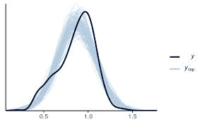
Suppose in particular that Nature’s data-generating process is $Y \mid X=x \sim \mathrm{N}$ $\left(7+x-0.03 x^2, 10^2\right)$, where $X \sim \mathrm{N}\left(15,5^2\right)$. A scatterplot of $n=1,000$ data values from this process is shown in the left panel of Figure 3.2, with OLS line and LOESS fit superimposed. Notice that the LOESS fit looks more like the true, quadratic function than the incorrect linear function.

The right panel of Figure 3.2 shows that the OLS estimates $\hat{\mu}_{15}=\hat{\beta}_0+\hat{\beta}_1(15)$, based on samples of size $n=1,000$, are biased (low) estimates of the true mean.

回归分析代写

统计代写|回归分析作业代写Regression Analysis代考|Unbiasedness of OLS Estimates Assuming the Classical Model: A Simulation Study

要开始模拟研究，必须指定模型及其参数值，在经典模型的情况下，这些参数值将是$\mathrm{N}\left(\beta_0+\beta_1 x, \sigma^2\right)$概率分布，以及三个参数$\left(\beta_0, \beta_1, \sigma\right)$。这些参数是未知的，所以只要选择任何有意义的值。无论你为这些参数选择什么值，你得到的估计都是(i)随机的，(ii)无偏的，在平均意义上既不高于也不低于这些参数值。

实际上，Nature会选择参数的实际值$\left(\beta_0, \beta_1, \sigma\right)$，而您并不知道它们的值。在模拟研究中，您选择值$\left(\beta_0, \beta_1, \sigma\right)$。估计值$\left(\hat{\beta}_0, \hat{\beta}_1\right.$和$\left.\hat{\sigma}\right)$针对这些特定的值，但是由于您既知道估计值又知道真实值，因此您可以精确地知道其中的误差。在现实世界中，使用真实(非模拟)数据，您的估计值$\hat{\beta}_0, \hat{\beta}_1$和$\hat{\sigma}$也针对真实值$\beta_0, \beta_1$和$\sigma$，但是由于您不知道真实数据的真实值，因此也不知道误差。模拟可以让您理解这个错误，因此您可以更好地理解您的估计$\hat{\beta}_0$、$\hat{\beta}_1$和$\hat{\sigma}$与Nature的真实值$\beta_0, \beta_1$和$\sigma$之间的关系。

在Production Cost示例中，值$\beta_0=55, \beta_1=1.5, \sigma^2=250^2$生成的数据看起来与实际数据非常相似，如第1章所示。让我们为模拟选择这些值。无论您为模拟参数$\beta_0, \beta_1$和$\sigma$选择哪个值，统计都会估计$\hat{\beta}_0, \hat{\beta}_1$和$\hat{\sigma}$“以”这些值为目标。

为了使抽象具体化和易于理解，运行下面的仿真代码，生成的数据如表3.3所示。
beta0 $=55 ;$ betal $=1.5 ;$ sigma $=250 #$自然参数
Widgets $=\mathrm{c}(1500,800,1500,1400,900,800,1400,1400,1300,1400,700$，
$\quad 1000,1200,1200,900,1200,1700,1600,1200,1400,1400,1000$，
$\quad 1200,800,1000,1400,1400,1500,1500,1600,1700,900,800,1300$，
$\quad 1000,1600,900,1300,1600,1000)$
n =长度(Widgets)
＃潜在可观察数据集的例子:
Sim。成本= beta0 + betal*Widgets + rnorm(n, 0, sigma)
head(cbind(Widgets, Sim.Cost))
beta $0=55 ;$ betal $=1.5 ;$ sigma $=250$ ＃自然参数
Widgets $=c(1500,800,1500,1400,900,800,1400,1400,1300,1400,700$，
$1000,1200,1200,900,1200,1700,1600,1200,1400,1400,1000$，
$1200,800,1000,1400,1400,1500,1500,1600,1700,900,800,1300$，
$1000,1600,900,1300,1600,1000)$
$\mathrm{n}=$长度(部件)
＃潜在可观察数据集的例子:
sim。成本$=$ beta $0+\operatorname{beta} 1 *$ widgets $+\operatorname{rnorm}(n, 0$, sigma $)$
head (cbind (Widgets, Sim.Cost))

统计代写|回归分析作业代写Regression Analysis代考|Biasedness of OLS Estimates When the Classical Model Is Wrong

当经典模型有效时，估计$\hat{\beta}_0$和$\hat{\beta}_1$的无偏性也意味着ols估计的条件平均值$\hat{\mu}_x=\hat{\beta}_0+\hat{\beta}_1 x$的无偏性。但是，当经典模型与自然模型不对应时，ols估计的条件平均值$\hat{\mu}_x=\hat{\beta}_0+\hat{\beta}_1 x$可能存在偏差。受图1.16的Product Complexity示例的启发，其中$Y=$ Preference和$X=$ Complexity假设Nature的均值函数不是线性的，而是一个曲线函数$\mathrm{E}(Y \mid X=x)=f(x)$。但你不知道自然的方式，所以你假设经典模型$Y \mid X=x \sim \mathrm{N}\left(\beta_0+\beta_1 x, \sigma^2\right)$。那么你的ols估计的条件平均值$\hat{\mu}_x=\hat{\beta}_0+\hat{\beta}_1 x$是有偏差的。

特别假设自然的数据生成过程是$Y \mid X=x \sim \mathrm{N}$$\left(7+x-0.03 x^2, 10^2\right)$，其中$X \sim \mathrm{N}\left(15,5^2\right)$。图3.2左面板为该过程中$n=1,000$数据值的散点图，OLS线与黄土拟合叠加。注意，黄土拟合看起来更像真实的二次函数，而不是不正确的线性函数。

图3.2的右面板显示，基于样本规模$n=1,000$的OLS估计$\hat{\mu}_{15}=\hat{\beta}_0+\hat{\beta}_1(15)$是对真实平均值的有偏(低)估计。

统计代写请认准statistics-lab™. statistics-lab™为您的留学生涯保驾护航。

随机过程代考

在概率论概念中，随机过程是随机变量的集合。 若一随机系统的样本点是随机函数，则称此函数为样本函数，这一随机系统全部样本函数的集合是一个随机过程。 实际应用中，样本函数的一般定义在时间域或者空间域。 随机过程的实例如股票和汇率的波动、语音信号、视频信号、体温的变化，随机运动如布朗运动、随机徘徊等等。

贝叶斯方法代考

贝叶斯统计概念及数据分析表示使用概率陈述回答有关未知参数的研究问题以及统计范式。后验分布包括关于参数的先验分布，和基于观测数据提供关于参数的信息似然模型。根据选择的先验分布和似然模型，后验分布可以解析或近似，例如，马尔科夫链蒙特卡罗 (MCMC) 方法之一。贝叶斯统计概念及数据分析使用后验分布来形成模型参数的各种摘要，包括点估计，如后验平均值、中位数、百分位数和称为可信区间的区间估计。此外，所有关于模型参数的统计检验都可以表示为基于估计后验分布的概率报表。

广义线性模型代考

广义线性模型（GLM）归属统计学领域，是一种应用灵活的线性回归模型。该模型允许因变量的偏差分布有除了正态分布之外的其它分布。

statistics-lab作为专业的留学生服务机构，多年来已为美国、英国、加拿大、澳洲等留学热门地的学生提供专业的学术服务，包括但不限于Essay代写，Assignment代写，Dissertation代写，Report代写，小组作业代写，Proposal代写，Paper代写，Presentation代写，计算机作业代写，论文修改和润色，网课代做，exam代考等等。写作范围涵盖高中，本科，研究生等海外留学全阶段，辐射金融，经济学，会计学，审计学，管理学等全球99%专业科目。写作团队既有专业英语母语作者，也有海外名校硕博留学生，每位写作老师都拥有过硬的语言能力，专业的学科背景和学术写作经验。我们承诺100%原创，100%专业，100%准时，100%满意。

机器学习代写

随着AI的大潮到来，Machine Learning逐渐成为一个新的学习热点。同时与传统CS相比，Machine Learning在其他领域也有着广泛的应用，因此这门学科成为不仅折磨CS专业同学的“小恶魔”，也是折磨生物、化学、统计等其他学科留学生的“大魔王”。学习Machine learning的一大绊脚石在于使用语言众多，跨学科范围广，所以学习起来尤其困难。但是不管你在学习Machine Learning时遇到任何难题，StudyGate专业导师团队都能为你轻松解决。

多元统计分析代考

基础数据: $N$ 个样本， $P$ 个变量数的单样本，组成的横列的数据表
变量定性: 分类和顺序；变量定量：数值
数学公式的角度分为: 因变量与自变量

时间序列分析代写

随机过程，是依赖于参数的一组随机变量的全体，参数通常是时间。 随机变量是随机现象的数量表现，其时间序列是一组按照时间发生先后顺序进行排列的数据点序列。通常一组时间序列的时间间隔为一恒定值（如1秒，5分钟，12小时，7天，1年），因此时间序列可以作为离散时间数据进行分析处理。研究时间序列数据的意义在于现实中，往往需要研究某个事物其随时间发展变化的规律。这就需要通过研究该事物过去发展的历史记录，以得到其自身发展的规律。

回归分析代写

多元回归分析渐进（Multiple Regression Analysis Asymptotics）属于计量经济学领域，主要是一种数学上的统计分析方法，可以分析复杂情况下各影响因素的数学关系，在自然科学、社会和经济学等多个领域内应用广泛。

MATLAB代写

MATLAB 是一种用于技术计算的高性能语言。它将计算、可视化和编程集成在一个易于使用的环境中，其中问题和解决方案以熟悉的数学符号表示。典型用途包括：数学和计算算法开发建模、仿真和原型制作数据分析、探索和可视化科学和工程图形应用程序开发，包括图形用户界面构建MATLAB 是一个交互式系统，其基本数据元素是一个不需要维度的数组。这使您可以解决许多技术计算问题，尤其是那些具有矩阵和向量公式的问题，而只需用 C 或 Fortran 等标量非交互式语言编写程序所需的时间的一小部分。MATLAB 名称代表矩阵实验室。MATLAB 最初的编写目的是提供对由 LINPACK 和 EISPACK 项目开发的矩阵软件的轻松访问，这两个项目共同代表了矩阵计算软件的最新技术。MATLAB 经过多年的发展，得到了许多用户的投入。在大学环境中，它是数学、工程和科学入门和高级课程的标准教学工具。在工业领域，MATLAB 是高效研究、开发和分析的首选工具。MATLAB 具有一系列称为工具箱的特定于应用程序的解决方案。对于大多数 MATLAB 用户来说非常重要，工具箱允许您学习和应用专业技术。工具箱是 MATLAB 函数（M 文件）的综合集合，可扩展 MATLAB 环境以解决特定类别的问题。可用工具箱的领域包括信号处理、控制系统、神经网络、模糊逻辑、小波、仿真等。

R语言代写	问卷设计与分析代写
PYTHON代写	回归分析与线性模型代写
MATLAB代写	方差分析与试验设计代写
STATA代写	机器学习/统计学习代写
SPSS代写	计量经济学代写
EVIEWS代写	时间序列分析代写
EXCEL代写	深度学习代写
SQL代写	各种数据建模与可视化代写

如果你也在 怎样代写回归分析Regression Analysis这个学科遇到相关的难题，请随时右上角联系我们的24/7代写客服。

回归分析是一种强大的统计方法，允许你检查两个或多个感兴趣的变量之间的关系。虽然有许多类型的回归分析，但它们的核心都是考察一个或多个自变量对因变量的影响。

statistics-lab™ 为您的留学生涯保驾护航 在代写回归分析Regression Analysis方面已经树立了自己的口碑, 保证靠谱, 高质且原创的统计Statistics代写服务。我们的专家在代写回归分析Regression Analysis代写方面经验极为丰富，各种代写回归分析Regression Analysis相关的作业也就用不着说。

统计代写|回归分析作业代写Regression Analysis代考|Estimating Regression Models via Maximum Likelihood

Table 1.3 of Chapter 1 is reproduced here as Table 2.1. This table shows how you should view regression data.

Table 2.1 also shows you how to get the likelihood function and the associated maximum likelihood estimates: Just plug the observed $y_i$ values into the conditional distributions and multiply them. Table 2.2 shows how you can obtain the likelihood function.
Now, under particular regression assumptions, each distribution $p\left(y \mid X=x_i\right)$ is a function of parameters $\boldsymbol{\theta}$, where $\boldsymbol{\theta}$ is a vector (or list) containing all the $\beta^{\prime}$ s and other parameters such as $\sigma$. Displaying this dependence explicitly, Table 2.2 becomes Table 2.3.

By assuming conditional independence of the potentially observable $Y_i \mid X_i=x_i$ observations, you then can multiply the individual likelihoods to get the joint likelihood as follows:
$$
L(\boldsymbol{\theta} \mid \text { data })=p\left(y_1 \mid X=x_1, \boldsymbol{\theta}\right) \times p\left(y_2 \mid X=x_2, \boldsymbol{\theta}\right) \times p\left(y_3 \mid X=x_3, \boldsymbol{\theta}\right) \times \ldots \times p\left(y_n \mid X=x_n, \boldsymbol{\theta}\right)
$$
To estimate the parameters $\boldsymbol{\theta}$ via maximum likelihood, you must identify the specific $\hat{\boldsymbol{\theta}}$ that maximizes $L(\boldsymbol{\theta} \mid$ data $)$. The resulting values of the vector $\hat{\boldsymbol{\theta}}$ are called the maximum likelihood estimates.

统计代写|回归分析作业代写Regression Analysis代考|Maximum Likelihood in the Classical (Normally Distributed) Regression Model, Which Gives You Ordinary Least Squares

When you assume the classical regression model (see Section 1.7), where the distributions are all normal, homoscedastic, and linked to $x$ linearly, the probability distributions $p(y \mid X=x)$ that you assume to produce your $Y \mid X=x$ data are the $\mathrm{N}\left(\beta_0+\beta_1 x, \sigma^2\right)$ distributions. These distributions have mathematical form given by:
$$
p(y \mid X=x, \theta)=p\left(y \mid X=x, \beta_0, \beta_1, \sigma\right)=\frac{1}{\sqrt{2 \pi} \sigma} \exp \left[-\frac{\left{y-\left(\beta_0+\beta_1 x\right)\right}^2}{2 \sigma^2}\right]
$$
You need this mathematical form to construct the likelihood function.
See Figure 1.7 (again!) for a graphic illustration of these models. Notice that the parameter vector is $\theta=\left{\beta_0, \beta_1, \sigma\right}$; i.e., there are three unknown parameters of this model that you must estimate using maximum likelihood. Assuming conditional independence, the likelihood function is

$$
\begin{aligned}
L(\theta \mid \text { data })= & p\left(y_1 \mid X=x_1, \theta\right) \times p\left(y_2 \mid X=x_2, \theta\right) \times \ldots \times p\left(y_n \mid X=x_n, \theta\right) \
= & \frac{1}{\sqrt{2 \pi} \sigma} \exp \left[-\frac{\left{y_1-\left(\beta_0+\beta_1 x_1\right)\right}^2}{2 \sigma^2}\right] \times \frac{1}{\sqrt{2 \pi} \sigma} \exp \left[-\frac{\left{y_2-\left(\beta_0+\beta_1 x_2\right)\right}^2}{2 \sigma^2}\right] \
& \times \cdots \times \frac{1}{\sqrt{2 \pi} \sigma} \exp \left[-\frac{\left{y_n-\left(\beta_0+\beta_1 x_n\right)\right}^2}{2 \sigma^2}\right] \
= & (2 \pi)^{-n / 2}\left(\sigma^2\right)^{-n / 2} \exp \left[-\frac{\sum_{i=1}^n\left{y_i-\left(\beta_0+\beta_1 x_i\right)\right}^2}{2 \sigma^2}\right]
\end{aligned}
$$
A technical note: In the random- $X$ case, the likelihood should also contain the multiplicative terms $p\left(x_1\right) \times p\left(x_2\right) \times \ldots \times p\left(x_n\right)$. But as long as $p(x)$ does not depend on the unknown parameters $\left(\beta_0, \beta_1, \sigma\right)$, these extra terms have no effect and are thus usually left off of the likelihood function.

Taking the logarithm of the likelihood function and simplifying, you get the loglikelihood function.
The log-likelihood function for the classical regression model
$$
L L(\theta \mid \text { data })=-\frac{n}{2} \ln (2 \pi)-\frac{n}{2} \ln \left(\sigma^2\right)-\frac{1}{2 \sigma^2} \sum_{i=1}^n\left{y_i-\left(\beta_0+\beta_1 x_i\right)\right}^2
$$

回归分析代写

统计代写|回归分析作业代写Regression Analysis代考|Estimating Regression Models via Maximum Likelihood

第1章表1.3在此复制为表2.1。此表显示了您应该如何查看回归数据。

表2.1还向您展示了如何获得似然函数和相关的最大似然估计:只需将观察到的$y_i$值插入条件分布并将它们相乘。表2.2显示了如何获得似然函数。
现在，在特定的回归假设下，每个分布$p\left(y \mid X=x_i\right)$是参数$\boldsymbol{\theta}$的函数，其中$\boldsymbol{\theta}$是包含所有$\beta^{\prime}$ s和其他参数(如$\sigma$)的向量(或列表)。显式显示这种依赖关系，表2.2变成了表2.3。

通过假设潜在可观察到的$Y_i \mid X_i=x_i$观测值的条件独立性，然后您可以将单个可能性相乘，得到如下所示的联合可能性:
$$
L(\boldsymbol{\theta} \mid \text { data })=p\left(y_1 \mid X=x_1, \boldsymbol{\theta}\right) \times p\left(y_2 \mid X=x_2, \boldsymbol{\theta}\right) \times p\left(y_3 \mid X=x_3, \boldsymbol{\theta}\right) \times \ldots \times p\left(y_n \mid X=x_n, \boldsymbol{\theta}\right)
$$
要通过最大似然估计参数$\boldsymbol{\theta}$，必须确定使$L(\boldsymbol{\theta} \mid$数据最大化的特定$\hat{\boldsymbol{\theta}}$$)$。向量$\hat{\boldsymbol{\theta}}$的结果值称为最大似然估计。

统计代写|回归分析作业代写Regression Analysis代考|Maximum Likelihood in the Classical (Normally Distributed) Regression Model, Which Gives You Ordinary Least Squares

当您假设经典回归模型(参见1.7节)，其中分布都是正态的、均方差的，并且与$x$线性关联，那么您假设产生$Y \mid X=x$数据的概率分布$p(y \mid X=x)$就是$\mathrm{N}\left(\beta_0+\beta_1 x, \sigma^2\right)$分布。这些分布的数学形式为:
$$
p(y \mid X=x, \theta)=p\left(y \mid X=x, \beta_0, \beta_1, \sigma\right)=\frac{1}{\sqrt{2 \pi} \sigma} \exp \left[-\frac{\left{y-\left(\beta_0+\beta_1 x\right)\right}^2}{2 \sigma^2}\right]
$$
你需要这种数学形式来构造似然函数。
参见图1.7(再次!)，以获得这些模型的图形说明。注意参数向量是$\theta=\left{\beta_0, \beta_1, \sigma\right}$;也就是说，这个模型有三个未知的参数，你必须使用最大似然来估计。假设条件无关，似然函数为

$$
\begin{aligned}
L(\theta \mid \text { data })= & p\left(y_1 \mid X=x_1, \theta\right) \times p\left(y_2 \mid X=x_2, \theta\right) \times \ldots \times p\left(y_n \mid X=x_n, \theta\right) \
= & \frac{1}{\sqrt{2 \pi} \sigma} \exp \left[-\frac{\left{y_1-\left(\beta_0+\beta_1 x_1\right)\right}^2}{2 \sigma^2}\right] \times \frac{1}{\sqrt{2 \pi} \sigma} \exp \left[-\frac{\left{y_2-\left(\beta_0+\beta_1 x_2\right)\right}^2}{2 \sigma^2}\right] \
& \times \cdots \times \frac{1}{\sqrt{2 \pi} \sigma} \exp \left[-\frac{\left{y_n-\left(\beta_0+\beta_1 x_n\right)\right}^2}{2 \sigma^2}\right] \
= & (2 \pi)^{-n / 2}\left(\sigma^2\right)^{-n / 2} \exp \left[-\frac{\sum_{i=1}^n\left{y_i-\left(\beta_0+\beta_1 x_i\right)\right}^2}{2 \sigma^2}\right]
\end{aligned}
$$
一个技术说明:在随机- $X$的情况下，似然也应该包含乘法项$p\left(x_1\right) \times p\left(x_2\right) \times \ldots \times p\left(x_n\right)$。但只要$p(x)$不依赖于未知参数$\left(\beta_0, \beta_1, \sigma\right)$，这些额外的项就没有影响，因此通常被排除在似然函数之外。

取似然函数的对数并化简，就得到了对数似然函数。
经典回归模型的对数似然函数
$$
L L(\theta \mid \text { data })=-\frac{n}{2} \ln (2 \pi)-\frac{n}{2} \ln \left(\sigma^2\right)-\frac{1}{2 \sigma^2} \sum_{i=1}^n\left{y_i-\left(\beta_0+\beta_1 x_i\right)\right}^2
$$

统计代写请认准statistics-lab™. statistics-lab™为您的留学生涯保驾护航。

随机过程代考

在概率论概念中，随机过程是随机变量的集合。 若一随机系统的样本点是随机函数，则称此函数为样本函数，这一随机系统全部样本函数的集合是一个随机过程。 实际应用中，样本函数的一般定义在时间域或者空间域。 随机过程的实例如股票和汇率的波动、语音信号、视频信号、体温的变化，随机运动如布朗运动、随机徘徊等等。

贝叶斯方法代考

贝叶斯统计概念及数据分析表示使用概率陈述回答有关未知参数的研究问题以及统计范式。后验分布包括关于参数的先验分布，和基于观测数据提供关于参数的信息似然模型。根据选择的先验分布和似然模型，后验分布可以解析或近似，例如，马尔科夫链蒙特卡罗 (MCMC) 方法之一。贝叶斯统计概念及数据分析使用后验分布来形成模型参数的各种摘要，包括点估计，如后验平均值、中位数、百分位数和称为可信区间的区间估计。此外，所有关于模型参数的统计检验都可以表示为基于估计后验分布的概率报表。

广义线性模型代考

广义线性模型（GLM）归属统计学领域，是一种应用灵活的线性回归模型。该模型允许因变量的偏差分布有除了正态分布之外的其它分布。

statistics-lab作为专业的留学生服务机构，多年来已为美国、英国、加拿大、澳洲等留学热门地的学生提供专业的学术服务，包括但不限于Essay代写，Assignment代写，Dissertation代写，Report代写，小组作业代写，Proposal代写，Paper代写，Presentation代写，计算机作业代写，论文修改和润色，网课代做，exam代考等等。写作范围涵盖高中，本科，研究生等海外留学全阶段，辐射金融，经济学，会计学，审计学，管理学等全球99%专业科目。写作团队既有专业英语母语作者，也有海外名校硕博留学生，每位写作老师都拥有过硬的语言能力，专业的学科背景和学术写作经验。我们承诺100%原创，100%专业，100%准时，100%满意。

机器学习代写

随着AI的大潮到来，Machine Learning逐渐成为一个新的学习热点。同时与传统CS相比，Machine Learning在其他领域也有着广泛的应用，因此这门学科成为不仅折磨CS专业同学的“小恶魔”，也是折磨生物、化学、统计等其他学科留学生的“大魔王”。学习Machine learning的一大绊脚石在于使用语言众多，跨学科范围广，所以学习起来尤其困难。但是不管你在学习Machine Learning时遇到任何难题，StudyGate专业导师团队都能为你轻松解决。

多元统计分析代考

基础数据: $N$ 个样本， $P$ 个变量数的单样本，组成的横列的数据表
变量定性: 分类和顺序；变量定量：数值
数学公式的角度分为: 因变量与自变量

时间序列分析代写

随机过程，是依赖于参数的一组随机变量的全体，参数通常是时间。 随机变量是随机现象的数量表现，其时间序列是一组按照时间发生先后顺序进行排列的数据点序列。通常一组时间序列的时间间隔为一恒定值（如1秒，5分钟，12小时，7天，1年），因此时间序列可以作为离散时间数据进行分析处理。研究时间序列数据的意义在于现实中，往往需要研究某个事物其随时间发展变化的规律。这就需要通过研究该事物过去发展的历史记录，以得到其自身发展的规律。

回归分析代写

多元回归分析渐进（Multiple Regression Analysis Asymptotics）属于计量经济学领域，主要是一种数学上的统计分析方法，可以分析复杂情况下各影响因素的数学关系，在自然科学、社会和经济学等多个领域内应用广泛。

MATLAB代写

MATLAB 是一种用于技术计算的高性能语言。它将计算、可视化和编程集成在一个易于使用的环境中，其中问题和解决方案以熟悉的数学符号表示。典型用途包括：数学和计算算法开发建模、仿真和原型制作数据分析、探索和可视化科学和工程图形应用程序开发，包括图形用户界面构建MATLAB 是一个交互式系统，其基本数据元素是一个不需要维度的数组。这使您可以解决许多技术计算问题，尤其是那些具有矩阵和向量公式的问题，而只需用 C 或 Fortran 等标量非交互式语言编写程序所需的时间的一小部分。MATLAB 名称代表矩阵实验室。MATLAB 最初的编写目的是提供对由 LINPACK 和 EISPACK 项目开发的矩阵软件的轻松访问，这两个项目共同代表了矩阵计算软件的最新技术。MATLAB 经过多年的发展，得到了许多用户的投入。在大学环境中，它是数学、工程和科学入门和高级课程的标准教学工具。在工业领域，MATLAB 是高效研究、开发和分析的首选工具。MATLAB 具有一系列称为工具箱的特定于应用程序的解决方案。对于大多数 MATLAB 用户来说非常重要，工具箱允许您学习和应用专业技术。工具箱是 MATLAB 函数（M 文件）的综合集合，可扩展 MATLAB 环境以解决特定类别的问题。可用工具箱的领域包括信号处理、控制系统、神经网络、模糊逻辑、小波、仿真等。

R语言代写	问卷设计与分析代写
PYTHON代写	回归分析与线性模型代写
MATLAB代写	方差分析与试验设计代写
STATA代写	机器学习/统计学习代写
SPSS代写	计量经济学代写
EVIEWS代写	时间序列分析代写
EXCEL代写	深度学习代写
SQL代写	各种数据建模与可视化代写

如果你也在 怎样代写线性回归分析linear regression analysis这个学科遇到相关的难题，请随时右上角联系我们的24/7代写客服。

回归分析是一种强大的统计方法，允许你检查两个或多个感兴趣的变量之间的关系。虽然有许多类型的回归分析，但它们的核心都是考察一个或多个自变量对因变量的影响。

statistics-lab™ 为您的留学生涯保驾护航 在代写线性回归分析linear regression analysis方面已经树立了自己的口碑, 保证靠谱, 高质且原创的统计Statistics代写服务。我们的专家在代写线性回归分析linear regression analysis代写方面经验极为丰富，各种代写线性回归分析linear regression analysis相关的作业也就用不着说。

我们提供的线性回归分析linear regression analysis及其相关学科的代写，服务范围广, 其中包括但不限于:

• Statistical Inference 统计推断
• Statistical Computing 统计计算
• Advanced Probability Theory 高等楖率论
• Advanced Mathematical Statistics 高等数理统计学
• (Generalized) Linear Models 广义线性模型
• Statistical Machine Learning 统计机器学习
• Longitudinal Data Analysis 纵向数据分析
• Foundations of Data Science 数据科学基础

统计代写|线性回归分析代写linear regression analysis代考|Correct Functional Specification

The conditional mean function is $f(x)=\mathrm{E}(Y \mid X=x)$, the collection of means of the conditional distributions $p(y \mid x)$ (a different mean for every $x$ ), viewed as a function of $x$. The conditional mean function $f(x)$ is the deterministic portion of the more general regression model $Y \mid X=x \sim p(y \mid x)$.
Definition of the true conditional mean function
The true conditional mean function is given by $f(x)=\mathrm{E}(Y \mid X=x)$.
Note that the true conditional mean function is different from the true regression model, which was already given in Section 1.1, but is repeated here to make the distinction clear.
Definition of the true regression model
The true regression model is given by $Y \mid X=x \sim p(y \mid x)$.
When the distributions $p(y \mid x)$ are continuous, you can obtain the true conditional mean function from the true regression model via $\mathrm{E}(Y \mid X=x)=\int y p(y \mid x) d y$. However, you cannot obtain the true regression model from the true conditional mean function, for the simple reason that you cannot tell anything about a distribution from its mean. For example, even if you know that the mean of $Y$ is 10.0 (for any $X=x$ ), you still do not know anything about the distribution of $Y$ (normal, lognormal, Poisson, etc.), or even its variance.
Whether you realize it or not, whenever you instruct the computer to analyze your regression data, you are making an assumption about the mean function. The correct functional specification assumption is simply the assumption that the mean function that you assume correctly specifies the true mean function of the data-generating process.
Correct functional specification assumption
The collection of true conditional means $f(x)=\mathrm{E}(Y \mid X=x)$ fall exactly on a function that is in the family of functions $f(x ; \boldsymbol{\beta})$ that you assume when you analyze your data, for some vector $\beta$ of fixed, unknown parameters.

统计代写|线性回归分析代写linear regression analysis代考|Constant Variance (Homoscedasticity)

The correct functional specification assumption refers to the means of the conditional distributions $p(y \mid x)$, as a function of $x$. The constant variance assumption refers to the variances of the conditional distributions $p(y \mid x)$, as a function of $x$. Letting $\mu_x=\mathrm{E}(Y \mid X=x)$, these conditional variances are calculated as $\sigma_x^2=\operatorname{Var}(Y \mid X=x)=\int_{\text {all } y}\left(y-\mu_x\right)^2 p(y \mid x) d y$.
Like the conditional mean function, the conditional variance function can have any function form in reality, linear, exponential, or any generic form whatsoever, provided that the function is non-negative. However, in the classical regression model, this function is assumed to have a very restrictive form: It is assumed to be a flat function that gives the same function value, regardless of the value of $x$.
The constant variance (homoscedasticity) assumption
The variances of the conditional distributions $p(y \mid x)$ are constant (i.e., they are all the same number, $\sigma^2$ ) for all specific values $X=x$.

Unlike the previous assumptions, which do not refer to any specific data set, this assumption refers to the data that you can collect, with observations $i=1,2, \ldots, n$.
Uncorrelated errors (or conditional independence) assumption
The potentially observable “error term,” $\varepsilon_i=Y_i-f\left(x_i ; \boldsymbol{\beta}\right)$, is uncorrelated with the potentially observable error $\varepsilon_j=Y_j-f\left(\boldsymbol{x}_j ; \boldsymbol{\beta}\right)$, for all sample pairs $(i, j), 1 \leq i, j \leq n$.
Alternatively, you can assume that the $Y_i$ are independent, given all the $X$ data. This alternative form is used in the construction of likelihood functions for maximum likelihood estimation and Bayesian analysis.

线性回归代写

统计代写|线性回归分析代写linear regression analysis代考|Correct Functional Specification

条件均值函数是$f(x)=\mathrm{E}(Y \mid X=x)$，是条件分布$p(y \mid x)$的均值的集合(每个$x$都有不同的均值)，可以看作是$x$的函数。条件平均函数$f(x)$是更一般的回归模型$Y \mid X=x \sim p(y \mid x)$的确定性部分。
真条件平均函数的定义
真实的条件平均函数由$f(x)=\mathrm{E}(Y \mid X=x)$给出。
请注意，真正的条件平均函数不同于真正的回归模型，这在1.1节中已经给出了，但在这里重复一遍，以明确区分。
真回归模型的定义
真实回归模型由$Y \mid X=x \sim p(y \mid x)$给出。
当分布$p(y \mid x)$连续时，可以通过$\mathrm{E}(Y \mid X=x)=\int y p(y \mid x) d y$从真回归模型中获得真条件均值函数。然而，你不能从真正的条件均值函数中得到真正的回归模型，原因很简单，你不能从一个分布的均值中得到任何信息。例如，即使您知道$Y$的平均值是10.0(对于任何$X=x$)，您仍然不知道$Y$的分布(正态、对数正态、泊松等)，甚至不知道它的方差。
不管你是否意识到，每当你让计算机分析你的回归数据时，你都是在对均值函数做一个假设。正确的功能规格假设只是假设您正确假设的平均函数指定了数据生成过程的真实平均函数。
正确的功能规格假设
true条件意味着$f(x)=\mathrm{E}(Y \mid X=x)$的集合恰好落在函数族$f(x ; \boldsymbol{\beta})$中的一个函数上，该函数是您在分析数据时假设的，用于某个具有固定未知参数的向量$\beta$。

统计代写|线性回归分析代写linear regression analysis代考|Constant Variance (Homoscedasticity)

正确的功能规范假设是指条件分布$p(y \mid x)$的均值，作为$x$的函数。常方差假设是指条件分布$p(y \mid x)$的方差，是$x$的函数。设$\mu_x=\mathrm{E}(Y \mid X=x)$，这些条件方差计算为$\sigma_x^2=\operatorname{Var}(Y \mid X=x)=\int_{\text {all } y}\left(y-\mu_x\right)^2 p(y \mid x) d y$。
就像条件均值函数一样，条件方差函数在现实中可以有任何函数形式，线性、指数或任何一般形式，只要函数是非负的。然而，在经典回归模型中，该函数被假定为具有非常严格的形式:假定它是一个平面函数，无论$x$的值如何，它都给出相同的函数值。
常方差(均方差)假设
对于所有特定值$X=x$，条件分布的方差$p(y \mid x)$是恒定的(即，它们都是相同的数字，$\sigma^2$)。

与前面的假设不同，前面的假设不涉及任何特定的数据集，这个假设涉及您可以通过观察$i=1,2, \ldots, n$收集到的数据。
不相关错误(或条件独立)假设
潜在可观察的“误差项”$\varepsilon_i=Y_i-f\left(x_i ; \boldsymbol{\beta}\right)$与所有样本对$(i, j), 1 \leq i, j \leq n$的潜在可观察误差$\varepsilon_j=Y_j-f\left(\boldsymbol{x}_j ; \boldsymbol{\beta}\right)$不相关。
或者，给定所有的$X$数据，您可以假设$Y_i$是独立的。这种替代形式用于构造最大似然估计和贝叶斯分析的似然函数。

统计代写请认准statistics-lab™. statistics-lab™为您的留学生涯保驾护航。

随机过程代考

在概率论概念中，随机过程是随机变量的集合。 若一随机系统的样本点是随机函数，则称此函数为样本函数，这一随机系统全部样本函数的集合是一个随机过程。 实际应用中，样本函数的一般定义在时间域或者空间域。 随机过程的实例如股票和汇率的波动、语音信号、视频信号、体温的变化，随机运动如布朗运动、随机徘徊等等。

贝叶斯方法代考

贝叶斯统计概念及数据分析表示使用概率陈述回答有关未知参数的研究问题以及统计范式。后验分布包括关于参数的先验分布，和基于观测数据提供关于参数的信息似然模型。根据选择的先验分布和似然模型，后验分布可以解析或近似，例如，马尔科夫链蒙特卡罗 (MCMC) 方法之一。贝叶斯统计概念及数据分析使用后验分布来形成模型参数的各种摘要，包括点估计，如后验平均值、中位数、百分位数和称为可信区间的区间估计。此外，所有关于模型参数的统计检验都可以表示为基于估计后验分布的概率报表。

广义线性模型代考

广义线性模型（GLM）归属统计学领域，是一种应用灵活的线性回归模型。该模型允许因变量的偏差分布有除了正态分布之外的其它分布。

statistics-lab作为专业的留学生服务机构，多年来已为美国、英国、加拿大、澳洲等留学热门地的学生提供专业的学术服务，包括但不限于Essay代写，Assignment代写，Dissertation代写，Report代写，小组作业代写，Proposal代写，Paper代写，Presentation代写，计算机作业代写，论文修改和润色，网课代做，exam代考等等。写作范围涵盖高中，本科，研究生等海外留学全阶段，辐射金融，经济学，会计学，审计学，管理学等全球99%专业科目。写作团队既有专业英语母语作者，也有海外名校硕博留学生，每位写作老师都拥有过硬的语言能力，专业的学科背景和学术写作经验。我们承诺100%原创，100%专业，100%准时，100%满意。

机器学习代写

随着AI的大潮到来，Machine Learning逐渐成为一个新的学习热点。同时与传统CS相比，Machine Learning在其他领域也有着广泛的应用，因此这门学科成为不仅折磨CS专业同学的“小恶魔”，也是折磨生物、化学、统计等其他学科留学生的“大魔王”。学习Machine learning的一大绊脚石在于使用语言众多，跨学科范围广，所以学习起来尤其困难。但是不管你在学习Machine Learning时遇到任何难题，StudyGate专业导师团队都能为你轻松解决。

多元统计分析代考

基础数据: $N$ 个样本， $P$ 个变量数的单样本，组成的横列的数据表
变量定性: 分类和顺序；变量定量：数值
数学公式的角度分为: 因变量与自变量

时间序列分析代写

随机过程，是依赖于参数的一组随机变量的全体，参数通常是时间。 随机变量是随机现象的数量表现，其时间序列是一组按照时间发生先后顺序进行排列的数据点序列。通常一组时间序列的时间间隔为一恒定值（如1秒，5分钟，12小时，7天，1年），因此时间序列可以作为离散时间数据进行分析处理。研究时间序列数据的意义在于现实中，往往需要研究某个事物其随时间发展变化的规律。这就需要通过研究该事物过去发展的历史记录，以得到其自身发展的规律。

回归分析代写

多元回归分析渐进（Multiple Regression Analysis Asymptotics）属于计量经济学领域，主要是一种数学上的统计分析方法，可以分析复杂情况下各影响因素的数学关系，在自然科学、社会和经济学等多个领域内应用广泛。

MATLAB代写

MATLAB 是一种用于技术计算的高性能语言。它将计算、可视化和编程集成在一个易于使用的环境中，其中问题和解决方案以熟悉的数学符号表示。典型用途包括：数学和计算算法开发建模、仿真和原型制作数据分析、探索和可视化科学和工程图形应用程序开发，包括图形用户界面构建MATLAB 是一个交互式系统，其基本数据元素是一个不需要维度的数组。这使您可以解决许多技术计算问题，尤其是那些具有矩阵和向量公式的问题，而只需用 C 或 Fortran 等标量非交互式语言编写程序所需的时间的一小部分。MATLAB 名称代表矩阵实验室。MATLAB 最初的编写目的是提供对由 LINPACK 和 EISPACK 项目开发的矩阵软件的轻松访问，这两个项目共同代表了矩阵计算软件的最新技术。MATLAB 经过多年的发展，得到了许多用户的投入。在大学环境中，它是数学、工程和科学入门和高级课程的标准教学工具。在工业领域，MATLAB 是高效研究、开发和分析的首选工具。MATLAB 具有一系列称为工具箱的特定于应用程序的解决方案。对于大多数 MATLAB 用户来说非常重要，工具箱允许您学习和应用专业技术。工具箱是 MATLAB 函数（M 文件）的综合集合，可扩展 MATLAB 环境以解决特定类别的问题。可用工具箱的领域包括信号处理、控制系统、神经网络、模糊逻辑、小波、仿真等。

R语言代写	问卷设计与分析代写
PYTHON代写	回归分析与线性模型代写
MATLAB代写	方差分析与试验设计代写
STATA代写	机器学习/统计学习代写
SPSS代写	计量经济学代写
EVIEWS代写	时间序列分析代写
EXCEL代写	深度学习代写
SQL代写	各种数据建模与可视化代写

如果你也在 怎样代写线性回归分析linear regression analysis这个学科遇到相关的难题，请随时右上角联系我们的24/7代写客服。

回归分析是一种强大的统计方法，允许你检查两个或多个感兴趣的变量之间的关系。虽然有许多类型的回归分析，但它们的核心都是考察一个或多个自变量对因变量的影响。

statistics-lab™ 为您的留学生涯保驾护航 在代写线性回归分析linear regression analysis方面已经树立了自己的口碑, 保证靠谱, 高质且原创的统计Statistics代写服务。我们的专家在代写线性回归分析linear regression analysis代写方面经验极为丰富，各种代写线性回归分析linear regression analysis相关的作业也就用不着说。

我们提供的线性回归分析linear regression analysis及其相关学科的代写，服务范围广, 其中包括但不限于:

• Statistical Inference 统计推断
• Statistical Computing 统计计算
• Advanced Probability Theory 高等楖率论
• Advanced Mathematical Statistics 高等数理统计学
• (Generalized) Linear Models 广义线性模型
• Statistical Machine Learning 统计机器学习
• Longitudinal Data Analysis 纵向数据分析
• Foundations of Data Science 数据科学基础

统计代写|线性回归分析代写linear regression analysis代考|Data Used in Regression Analysis

A typical data set used in simple regression analysis looks as shown in Table 1.2.
In Table 1.2, “Obs” refers to “observation number.” It is important to recognize what the observations refer to, because the regression model $p(y \mid x)$ describes variation in $Y$ at that level of observation, as discussed in the following examples. For example, with person-level data, each “Obs” is a different person, person 1, person 2, etc. The variation in $Y$ modeled by $p(y \mid x)$ refers to variation between people. For example, $p(y \mid X=27)$ might refer to the potentially observable variation in Assets among people who are 27 years old. With firm-level data, each “Obs” is a different firm, e.g. firm 1 is Pfizer, firm 2 is Microsoft, etc., and the variation in $Y$ modeled by $p(y \mid x)$ refers to variation between firms. For example, $p(y \mid X=2,000)$ might refer to the potentially observable variation in net worth among firms that have 2,000 employees.

As a reminder, it is essential for understanding this entire book, to always remember the following two points:
The regression model $p(y \mid x)$ does not come from the data. Rather, the regression model $p(y \mid x)$ is assumed to produce the data.
To illustrate the crucial concept that the regression model is a producer of data, consider the data set, available in R, called “EuStockMarkets,” having Daily Closing Prices of Major European Stock Indices, from 1991 to 1998. These data are time-series data, where the “Obs” are consecutive trading days.

data (EustockMarkets)
$>\operatorname{tail}$ (EuStockMarkets $[, 1: 2])[1: 5$,
DAX SMI
$[1855] 5598.32 \quad$,
$[1856]$,
$[1857] 5285.78 \quad$,
$[1858] 5386.94 \quad$,
$[1859]$,
[1860,] 5473.72 ?????

统计代写|线性回归分析代写linear regression analysis代考|The Trashcan Experiment: Random- $X$ Versus Fixed- $X$

Here is something you can do (or at least imagine doing) with a group of people. You need a crumpled piece of paper (call it a “ball”), a tape measure, and a clean trashcan. Let each person attempt to throw the ball into the trashcan. The goal of the study is to identify the relationship between success at throwing the ball into the trash can $(Y)$, and distance from the trashcan $(X)$.

In a fixed- $X$ version of the experiment, place markers 5 feet, 10 feet, 15 feet and 20 feet from the trashcan. Have all people attempt to throw the ball into the trashcan from all those distances. Here the $X$ ‘s are fixed because they are known in advance. If you imagine doing another experiment just like this one (say in a different class), then the X’s would be the same: $5,10,15$ and 20.

In a random- $X$ version of the same experiment, you give a person the ball, then tell the person to pick a spot where he or she thinks the probability of making the shot might be around $50 \%$. Have the person attempt to throw the ball into the trashcan multiple times from that distance that he or she selected. Repeat for all people, letting each person pick where they want to stand. Here the X’s are random because they are not known in advance. If you imagine doing another experiment just like this one (say in a different class), then the X’s would be different because different people will choose different places to stand.

The fixed- $X$ version gives rise to experimental data. In experiments, the experimenter first sets the $X$ and then observes the $Y$. The random- $X$ version gives rise to observational data, where the X’s are simply observed, and not controlled by the researcher.

Experimental data are the gold standard, because with observational data the observed effect of $X$ on $Y$ may not be a causal effect. With experimental data, the observed effect of $X$ on $Y$ can be more easily interpreted as a causal effect. Issues of causality in more detail in later chapters.

线性回归代写

统计代写|线性回归分析代写linear regression analysis代考|Data Used in Regression Analysis

简单回归分析中使用的典型数据集如表1.2所示。
表1.2中“Obs”为“观测数”。重要的是要认识到观测值指的是什么，因为回归模型p(y \mid x)描述了在该观测水平上y $的变化，如下面的示例所述。例如，对于个人级别的数据，每个“Obs”是一个不同的人，人1、人2等等。由p(Y \mid x)$模拟的Y$的变化是指人与人之间的变化。例如，$p(y \mid X=27)$可能指的是27岁人群中潜在的可观察到的资产变化。对于公司层面的数据，每个“Obs”是一个不同的公司，例如公司1是辉瑞公司，公司2是微软公司，等等，而由p(Y \mid x)$建模的$Y$的变化指的是公司之间的变化。例如，$p(y \mid X=2,000)$可能指的是拥有2,000名员工的公司之间潜在的可观察到的净值变化。

提醒一下，要理解整本书，必须记住以下两点:
回归模型$p(y \mid x)$不是来自数据。相反，假设回归模型p(y \mid x)$产生数据。
为了说明回归模型是数据生产者的关键概念，考虑R中可用的数据集，称为“EuStockMarkets”，其中包含1991年至1998年欧洲主要股票指数的每日收盘价。这些数据是时间序列数据，其中“Obs”是连续的交易日。

数据(EustockMarkets)
$ > \ operatorname{尾巴}$(美元EuStockMarkets[1: 2])[1: 5美元,
DAX重度
$[1855] 5598.32 \quad$，
[1856],美元
$[1857] 5285.78 \quad$
$[1858] $ $，
[1859],美元
[1860，] 5473.72 ?????

统计代写|线性回归分析代写linear regression analysis代考|The Trashcan Experiment: Random- $X$ Versus Fixed- $X$

这里有一些你可以和一群人一起做(或者至少想象一下)的事情。你需要一张皱巴巴的纸(叫它“球”)，一个卷尺和一个干净的垃圾桶。让每个人试着把球扔进垃圾桶。这项研究的目的是确定成功将球扔进垃圾桶$(Y)$和距离垃圾桶$(X)$之间的关系。

在一个固定的X版本的实验中，在距离垃圾桶5英尺、10英尺、15英尺和20英尺的地方放置标记。让所有的人都试着把球扔进垃圾桶。这里的X是固定的，因为它们是提前知道的。如果你想象做另一个和这个实验一样的实验(比如在不同的课堂上)，那么X将是相同的:5美元、10美元、15美元和20美元。

在同一实验的随机版本中，你给一个人一个球，然后告诉这个人选择一个他或她认为投中概率在50%左右的位置。让这个人尝试从他或她选择的距离将球扔进垃圾桶多次。对所有人重复一遍，让每个人选择自己想站的位置。这里的X是随机的，因为它们事先不知道。如果你想象做另一个和这个实验一样的实验(比如在不同的课堂上)，那么X就会不同，因为不同的人会选择不同的站立位置。

固定$X$版本产生实验数据。在实验中，实验者首先设置X，然后观察Y。随机- $X$版本产生了观测数据，其中X只是被观察到，而不是由研究人员控制。

实验数据是金标准，因为对于观测数据，观察到的X对Y的影响可能不是因果关系。根据实验数据，观察到的X对Y的影响可以更容易地解释为因果效应。因果关系的问题将在后面的章节中详细讨论。

统计代写请认准statistics-lab™. statistics-lab™为您的留学生涯保驾护航。

随机过程代考

在概率论概念中，随机过程是随机变量的集合。 若一随机系统的样本点是随机函数，则称此函数为样本函数，这一随机系统全部样本函数的集合是一个随机过程。 实际应用中，样本函数的一般定义在时间域或者空间域。 随机过程的实例如股票和汇率的波动、语音信号、视频信号、体温的变化，随机运动如布朗运动、随机徘徊等等。

贝叶斯方法代考

贝叶斯统计概念及数据分析表示使用概率陈述回答有关未知参数的研究问题以及统计范式。后验分布包括关于参数的先验分布，和基于观测数据提供关于参数的信息似然模型。根据选择的先验分布和似然模型，后验分布可以解析或近似，例如，马尔科夫链蒙特卡罗 (MCMC) 方法之一。贝叶斯统计概念及数据分析使用后验分布来形成模型参数的各种摘要，包括点估计，如后验平均值、中位数、百分位数和称为可信区间的区间估计。此外，所有关于模型参数的统计检验都可以表示为基于估计后验分布的概率报表。

广义线性模型代考

广义线性模型（GLM）归属统计学领域，是一种应用灵活的线性回归模型。该模型允许因变量的偏差分布有除了正态分布之外的其它分布。

statistics-lab作为专业的留学生服务机构，多年来已为美国、英国、加拿大、澳洲等留学热门地的学生提供专业的学术服务，包括但不限于Essay代写，Assignment代写，Dissertation代写，Report代写，小组作业代写，Proposal代写，Paper代写，Presentation代写，计算机作业代写，论文修改和润色，网课代做，exam代考等等。写作范围涵盖高中，本科，研究生等海外留学全阶段，辐射金融，经济学，会计学，审计学，管理学等全球99%专业科目。写作团队既有专业英语母语作者，也有海外名校硕博留学生，每位写作老师都拥有过硬的语言能力，专业的学科背景和学术写作经验。我们承诺100%原创，100%专业，100%准时，100%满意。

机器学习代写

随着AI的大潮到来，Machine Learning逐渐成为一个新的学习热点。同时与传统CS相比，Machine Learning在其他领域也有着广泛的应用，因此这门学科成为不仅折磨CS专业同学的“小恶魔”，也是折磨生物、化学、统计等其他学科留学生的“大魔王”。学习Machine learning的一大绊脚石在于使用语言众多，跨学科范围广，所以学习起来尤其困难。但是不管你在学习Machine Learning时遇到任何难题，StudyGate专业导师团队都能为你轻松解决。

多元统计分析代考

基础数据: $N$ 个样本， $P$ 个变量数的单样本，组成的横列的数据表
变量定性: 分类和顺序；变量定量：数值
数学公式的角度分为: 因变量与自变量

时间序列分析代写

随机过程，是依赖于参数的一组随机变量的全体，参数通常是时间。 随机变量是随机现象的数量表现，其时间序列是一组按照时间发生先后顺序进行排列的数据点序列。通常一组时间序列的时间间隔为一恒定值（如1秒，5分钟，12小时，7天，1年），因此时间序列可以作为离散时间数据进行分析处理。研究时间序列数据的意义在于现实中，往往需要研究某个事物其随时间发展变化的规律。这就需要通过研究该事物过去发展的历史记录，以得到其自身发展的规律。

回归分析代写

多元回归分析渐进（Multiple Regression Analysis Asymptotics）属于计量经济学领域，主要是一种数学上的统计分析方法，可以分析复杂情况下各影响因素的数学关系，在自然科学、社会和经济学等多个领域内应用广泛。

MATLAB代写

MATLAB 是一种用于技术计算的高性能语言。它将计算、可视化和编程集成在一个易于使用的环境中，其中问题和解决方案以熟悉的数学符号表示。典型用途包括：数学和计算算法开发建模、仿真和原型制作数据分析、探索和可视化科学和工程图形应用程序开发，包括图形用户界面构建MATLAB 是一个交互式系统，其基本数据元素是一个不需要维度的数组。这使您可以解决许多技术计算问题，尤其是那些具有矩阵和向量公式的问题，而只需用 C 或 Fortran 等标量非交互式语言编写程序所需的时间的一小部分。MATLAB 名称代表矩阵实验室。MATLAB 最初的编写目的是提供对由 LINPACK 和 EISPACK 项目开发的矩阵软件的轻松访问，这两个项目共同代表了矩阵计算软件的最新技术。MATLAB 经过多年的发展，得到了许多用户的投入。在大学环境中，它是数学、工程和科学入门和高级课程的标准教学工具。在工业领域，MATLAB 是高效研究、开发和分析的首选工具。MATLAB 具有一系列称为工具箱的特定于应用程序的解决方案。对于大多数 MATLAB 用户来说非常重要，工具箱允许您学习和应用专业技术。工具箱是 MATLAB 函数（M 文件）的综合集合，可扩展 MATLAB 环境以解决特定类别的问题。可用工具箱的领域包括信号处理、控制系统、神经网络、模糊逻辑、小波、仿真等。

R语言代写	问卷设计与分析代写
PYTHON代写	回归分析与线性模型代写
MATLAB代写	方差分析与试验设计代写
STATA代写	机器学习/统计学习代写
SPSS代写	计量经济学代写
EVIEWS代写	时间序列分析代写
EXCEL代写	深度学习代写
SQL代写	各种数据建模与可视化代写

如果你也在 怎样代写线性回归分析linear regression analysis这个学科遇到相关的难题，请随时右上角联系我们的24/7代写客服。

回归分析是一种强大的统计方法，允许你检查两个或多个感兴趣的变量之间的关系。虽然有许多类型的回归分析，但它们的核心都是考察一个或多个自变量对因变量的影响。

statistics-lab™ 为您的留学生涯保驾护航 在代写线性回归分析linear regression analysis方面已经树立了自己的口碑, 保证靠谱, 高质且原创的统计Statistics代写服务。我们的专家在代写线性回归分析linear regression analysis代写方面经验极为丰富，各种代写线性回归分析linear regression analysis相关的作业也就用不着说。

我们提供的线性回归分析linear regression analysis及其相关学科的代写，服务范围广, 其中包括但不限于:

• Statistical Inference 统计推断
• Statistical Computing 统计计算
• Advanced Probability Theory 高等楖率论
• Advanced Mathematical Statistics 高等数理统计学
• (Generalized) Linear Models 广义线性模型
• Statistical Machine Learning 统计机器学习
• Longitudinal Data Analysis 纵向数据分析
• Foundations of Data Science 数据科学基础

统计代写|线性回归分析代写linear regression analysis代考|What does an insignificant estimate tell you

The basic reason why the lack of evidence is not proof of non-existence is that there are alternative reasons for the lack of evidence. As mentioned earlier, when a jury in a criminal trial deliberates on whether a defendant is guilty, the jury members are not directed to conclude that the defendant has been proven innocent. Rather, they are supposed to determine whether there is significant evidence (beyond a reasonable doubt) that indicates the defendant was guilty. Thus, one reason why a defendant may be found “not guilty” is that there was not enough evidence.

The same concept is supposed to be used for statistical analysis. We are often testing whether a coefficient estimate is different from zero. Let’s say we are examining how class-size affects elementary-school students’ test scores, and let’s say that we find an insignificant estimate on the variable for class-size. In a study of mine (Arkes 2016), I list four general possible explanations for an insignificant estimate:

1. There is actually no effect of the explanatory variable on the outcome in the population.
2. There is an effect in one direction, but the model is unable to detect the effect due to a modeling problem (e.g., omitted-factors bias or measurement error – see Chapter 6) biasing the coefficient estimate in a direction opposite to the actual effect.

3. There is a small effect that cannot be detected with the available data due to inadequate power i.e., not a large enough sample given the size of the effect.
4. There are varying effects in the population (or sample); some people’s outcomes may be affected positively by the treatment, others’ outcomes may be affected negatively, and others’ outcomes may not be affected; and the estimated effect (which is the average effect) is insignificantly different from zero due to the positive and negative effects canceling each other out or being drowned out by those with zero effects.

So what can you conclude from the insignificant estimate on the class-size variable? You cannot conclude that class size does not affect test scores. Rather, as with the hot hand and the search for aliens, the interpretation should be: “There is no evidence that class-size affects test scores.”

Unfortunately, a very common mistake made in the research world is that the conclusion would be that there is no effect. This is important for issues such as whether there are side effects from pharmaceutical drugs or vaccines. The lack of evidence for a side effect does not mean that there is no effect, particularly if confidence intervals for the estimates include values that would represent meaningful side effects of the drug or vaccine.

All that said, there are sometimes cases in which an insignificant estimate has a $95 \%$ or $99 \%$ confidence interval with a fairly narrow range and outer boundary that, if the boundary were the true population parameter, it would be “practically insignificant” (see Section 5.3.9). If this were the case and the coefficient estimate were not subject to any meaningful bias, then it would be safe to conclude that “there is no meaningful effect.”

统计代写|线性回归分析代写linear regression analysis代考|Statistical significance is not the goal

As we conduct research, our ultimate goal should be to advance knowledge. Our goal should not be to find a statistically-significant estimate. Advancing knowledge occurs by conducting objective and honest research.

A statistically insignificant coefficient estimate on a key-explanatory variable is just as valid as a significant coefficient estimate. The problem, many believe, is that an insignificant estimate may not provide as much information as a significant estimate. As described in the previous section, an insignificant estimate does not necessarily mean that there is no meaningful relationship, and so it could have multiple possible interpretations. If the appropriate confidence intervals for the coefficient were narrow (which would indicate adequate power), the methods were convincing for ruling out modeling problems, and the effects would likely go in just one direction, then it would be more reasonable to conclude that an insignificant estimate indicates there is no meaningful effect of the treatment. But meeting all those conditions is rare, and so there are multiple possible conclusions that cannot be distinguished.

As mentioned in the previous section, a statistically-significant estimate could also be subject to the various interpretations of insignificant estimates. But these are often ignored and not deemed as important, to most people, as long as there is statistical significance.

Statistical significance is valued more, perhaps, because it is evidence confirming, to some extent, the researcher’s theory and/or hypothesis. I conducted a quick, informal review of recent issues of leading economic, financial, and education journals. As it has been historically, almost all empirical studies had statistically-significant coefficient estimates on the key-explanatory variable. Indeed, I had a difficult time finding an insignificant estimate. This suggests that the pattern continues that journals are more likely to publish studies with significant estimates on the key-explanatory variables.

The result of statistical significance being valued more is that it incentivizes researchers to make statistical significance the goal of research. This can lead to $\mathbf{p}$-hacking, which involves changing the set of control variables, the method (e.g. Ordinary Least Squares (OLS) vs. an alternative method, such as in Chapters 8 and 9), the sample requirements, or how the variables (including the outcome) are defined until one achieves a p-value below a major threshold. (I describe p-hacking in more detail in Section 13.3.)

It is unfortunate that insignificant estimates are not accepted more. But, hopefully, this book will be another stepping stone for the movement to be more accepting of insignificant estimates. I personally trust insignificant estimates more than significant estimates (except for the hot hand in basketball).

The bottom line is that, as we conduct research, we should be guided by proper modeling strategies and not by what the results are saying.

线性回归代写

统计代写|线性回归分析代写linear regression analysis代考|What does an insignificant estimate tell you

缺乏证据不能证明不存在的基本原因是缺乏证据还有其他原因。如前所述，当陪审团在刑事审判中审议被告是否有罪时，陪审团成员并没有被指示得出被告已被证明无罪的结论。相反，他们应该确定是否有重要证据（排除合理怀疑）表明被告有罪。因此，被告人可能被判“无罪”的原因之一是证据不足。

同样的概念应该用于统计分析。我们经常测试系数估计值是否不同于零。假设我们正在研究班级规模如何影响小学生的考试成绩，假设我们发现班级规模变量的估计值不显着。在我的一项研究中（Arkes 2016），我列出了对微不足道的估计的四种一般可能解释：

1. 实际上，解释变量对总体结果没有影响。
2. 在一个方向上有影响，但由于建模问题（例如，遗漏因素偏差或测量误差——参见第 6 章），模型无法检测到影响系数估计值在与实际影响相反的方向上的偏差。

3. 由于功效不足，即没有足够大的样本给定效应大小，因此无法用可用数据检测到一个小效应。
4. 总体（或样本）有不同的影响；某些人的结果可能会受到治疗的积极影响，其他人的结果可能会受到负面影响，而其他人的结果可能不会受到影响；由于正负效应相互抵消或被零效应淹没，因此估计效应（即平均效应）与零无显着差异。

那么，从对班级规模变量的微不足道的估计中，你能得出什么结论呢？您不能断定班级规模不会影响考试成绩。相反，就像热手和寻找外星人一样，解释应该是：“没有证据表明班级规模会影响考试成绩。”

不幸的是，研究界常犯的一个错误是得出的结论是没有效果。这对于诸如药物或疫苗是否有副作用等问题很重要。缺乏副作用的证据并不意味着没有影响，特别是如果估计的置信区间包括代表药物或疫苗有意义的副作用的值。

综上所述，有时在某些情况下，微不足道的估计会产生95%或者99%具有相当窄的范围和外部边界的置信区间，如果边界是真实的人口参数，它将“实际上微不足道”（见第 5.3.9 节）。如果情况确实如此，并且系数估计不受任何有意义的偏差影响，那么可以安全地得出“没有有意义的影响”的结论。

统计代写|线性回归分析代写linear regression analysis代考|Statistical significance is not the goal

当我们进行研究时，我们的最终目标应该是增进知识。我们的目标不应该是找到具有统计意义的估计值。通过进行客观和诚实的研究来提高知识。

对关键解释变量的统计上不显着的系数估计与显着的系数估计一样有效。许多人认为，问题在于微不足道的估计可能无法提供与重要估计一样多的信息。如前一节所述，一个无关紧要的估计并不一定意味着没有有意义的关系，因此它可能有多种可能的解释。如果系数的适当置信区间较窄（这表明有足够的功效），这些方法对于排除建模问题是有说服力的，并且效果可能只朝一个方向发展，那么得出不显着的结论会更合理估计表明治疗没有有意义的效果。但满足所有这些条件是罕见的，

如前一节所述，具有统计意义的估计也可能受到对不重要估计的各种解释的影响。但对大多数人来说，只要具有统计显着性，这些往往会被忽略并且不被视为重要。

统计显着性更受重视，也许是因为它是在某种程度上证实研究人员的理论和/或假设的证据。我对最近几期领先的经济、金融和教育期刊进行了快速、非正式的审查。从历史上看，几乎所有的实证研究都对关键解释变量进行了统计显着的系数估计。事实上，我很难找到一个微不足道的估计。这表明该模式继续存在，即期刊更有可能发表对关键解释变量进行重大估计的研究。

统计显着性被更加重视的结果是它激励研究者将统计显着性作为研究的目标。这会导致p-hacking，涉及更改控制变量集、方法（例如普通最小二乘法 (OLS) 与替代方法，例如第 8 章和第 9 章中的方法）、样本要求或变量（包括结果）的变化方式被定义，直到一个人达到低于主要阈值的 p 值。（我在第 13.3 节中更详细地描述了 p-hacking。）

不幸的是，微不足道的估计不被更多人接受。但是，希望这本书将成为该运动更多地接受微不足道的估计的另一个垫脚石。我个人更相信无关紧要的估计而不是重要的估计（除了篮球中的热手）。

底线是，在我们进行研究时，我们应该以适当的建模策略为指导，而不是以结果的说法为指导。

统计代写请认准statistics-lab™. statistics-lab™为您的留学生涯保驾护航。

随机过程代考

在概率论概念中，随机过程是随机变量的集合。 若一随机系统的样本点是随机函数，则称此函数为样本函数，这一随机系统全部样本函数的集合是一个随机过程。 实际应用中，样本函数的一般定义在时间域或者空间域。 随机过程的实例如股票和汇率的波动、语音信号、视频信号、体温的变化，随机运动如布朗运动、随机徘徊等等。

贝叶斯方法代考

贝叶斯统计概念及数据分析表示使用概率陈述回答有关未知参数的研究问题以及统计范式。后验分布包括关于参数的先验分布，和基于观测数据提供关于参数的信息似然模型。根据选择的先验分布和似然模型，后验分布可以解析或近似，例如，马尔科夫链蒙特卡罗 (MCMC) 方法之一。贝叶斯统计概念及数据分析使用后验分布来形成模型参数的各种摘要，包括点估计，如后验平均值、中位数、百分位数和称为可信区间的区间估计。此外，所有关于模型参数的统计检验都可以表示为基于估计后验分布的概率报表。

广义线性模型代考

广义线性模型（GLM）归属统计学领域，是一种应用灵活的线性回归模型。该模型允许因变量的偏差分布有除了正态分布之外的其它分布。

statistics-lab作为专业的留学生服务机构，多年来已为美国、英国、加拿大、澳洲等留学热门地的学生提供专业的学术服务，包括但不限于Essay代写，Assignment代写，Dissertation代写，Report代写，小组作业代写，Proposal代写，Paper代写，Presentation代写，计算机作业代写，论文修改和润色，网课代做，exam代考等等。写作范围涵盖高中，本科，研究生等海外留学全阶段，辐射金融，经济学，会计学，审计学，管理学等全球99%专业科目。写作团队既有专业英语母语作者，也有海外名校硕博留学生，每位写作老师都拥有过硬的语言能力，专业的学科背景和学术写作经验。我们承诺100%原创，100%专业，100%准时，100%满意。

机器学习代写

随着AI的大潮到来，Machine Learning逐渐成为一个新的学习热点。同时与传统CS相比，Machine Learning在其他领域也有着广泛的应用，因此这门学科成为不仅折磨CS专业同学的“小恶魔”，也是折磨生物、化学、统计等其他学科留学生的“大魔王”。学习Machine learning的一大绊脚石在于使用语言众多，跨学科范围广，所以学习起来尤其困难。但是不管你在学习Machine Learning时遇到任何难题，StudyGate专业导师团队都能为你轻松解决。

多元统计分析代考

基础数据: $N$ 个样本， $P$ 个变量数的单样本，组成的横列的数据表
变量定性: 分类和顺序；变量定量：数值
数学公式的角度分为: 因变量与自变量

时间序列分析代写

随机过程，是依赖于参数的一组随机变量的全体，参数通常是时间。 随机变量是随机现象的数量表现，其时间序列是一组按照时间发生先后顺序进行排列的数据点序列。通常一组时间序列的时间间隔为一恒定值（如1秒，5分钟，12小时，7天，1年），因此时间序列可以作为离散时间数据进行分析处理。研究时间序列数据的意义在于现实中，往往需要研究某个事物其随时间发展变化的规律。这就需要通过研究该事物过去发展的历史记录，以得到其自身发展的规律。

回归分析代写

多元回归分析渐进（Multiple Regression Analysis Asymptotics）属于计量经济学领域，主要是一种数学上的统计分析方法，可以分析复杂情况下各影响因素的数学关系，在自然科学、社会和经济学等多个领域内应用广泛。

MATLAB代写

MATLAB 是一种用于技术计算的高性能语言。它将计算、可视化和编程集成在一个易于使用的环境中，其中问题和解决方案以熟悉的数学符号表示。典型用途包括：数学和计算算法开发建模、仿真和原型制作数据分析、探索和可视化科学和工程图形应用程序开发，包括图形用户界面构建MATLAB 是一个交互式系统，其基本数据元素是一个不需要维度的数组。这使您可以解决许多技术计算问题，尤其是那些具有矩阵和向量公式的问题，而只需用 C 或 Fortran 等标量非交互式语言编写程序所需的时间的一小部分。MATLAB 名称代表矩阵实验室。MATLAB 最初的编写目的是提供对由 LINPACK 和 EISPACK 项目开发的矩阵软件的轻松访问，这两个项目共同代表了矩阵计算软件的最新技术。MATLAB 经过多年的发展，得到了许多用户的投入。在大学环境中，它是数学、工程和科学入门和高级课程的标准教学工具。在工业领域，MATLAB 是高效研究、开发和分析的首选工具。MATLAB 具有一系列称为工具箱的特定于应用程序的解决方案。对于大多数 MATLAB 用户来说非常重要，工具箱允许您学习和应用专业技术。工具箱是 MATLAB 函数（M 文件）的综合集合，可扩展 MATLAB 环境以解决特定类别的问题。可用工具箱的领域包括信号处理、控制系统、神经网络、模糊逻辑、小波、仿真等。

R语言代写	问卷设计与分析代写
PYTHON代写	回归分析与线性模型代写
MATLAB代写	方差分析与试验设计代写
STATA代写	机器学习/统计学习代写
SPSS代写	计量经济学代写
EVIEWS代写	时间序列分析代写
EXCEL代写	深度学习代写
SQL代写	各种数据建模与可视化代写

如果你也在 怎样代写线性回归分析linear regression analysis这个学科遇到相关的难题，请随时右上角联系我们的24/7代写客服。

回归分析是一种强大的统计方法，允许你检查两个或多个感兴趣的变量之间的关系。虽然有许多类型的回归分析，但它们的核心都是考察一个或多个自变量对因变量的影响。

statistics-lab™ 为您的留学生涯保驾护航 在代写线性回归分析linear regression analysis方面已经树立了自己的口碑, 保证靠谱, 高质且原创的统计Statistics代写服务。我们的专家在代写线性回归分析linear regression analysis代写方面经验极为丰富，各种代写线性回归分析linear regression analysis相关的作业也就用不着说。

我们提供的线性回归分析linear regression analysis及其相关学科的代写，服务范围广, 其中包括但不限于:

• Statistical Inference 统计推断
• Statistical Computing 统计计算
• Advanced Probability Theory 高等楖率论
• Advanced Mathematical Statistics 高等数理统计学
• (Generalized) Linear Models 广义线性模型
• Statistical Machine Learning 统计机器学习
• Longitudinal Data Analysis 纵向数据分析
• Foundations of Data Science 数据科学基础

统计代写|线性回归分析代写linear regression analysis代考|What model diagnostics should you do?

None! Well, most of the time, none. This is my view, and I might be wrong. Others (including your professor) may have valid reasons to disagree. But here is the argument why, in most cases, there is no need to perform any model diagnostics.
The two most common model diagnostics that are conducted are:

• checking for heteroskedasticity
• checking for non-normal error terms (Assumption A3 in Section 2.10).
  One problem is that the tests are not great. The tests will indicate whether there is statisticallysignificant evidence for heteroskedasticity or non-normal error terms, but they certainly cannot prove that there is not any heteroskedasticity or non-normal error terms.

Regarding heteroskedasticity, your regression probably has heteroskedasticity. And, given that it is costless and painless to fix, you should probably include the heteroskedasticity correction.

Regarding non-normal error terms, recall that, due to the Central Limit Theorem, error terms will be approximately normal if the sample size is large enough (i.e., at least 200 observations at worst, and perhaps only 15 observations would suffice). However, this is not necessarily the case if: (1) the dependent variable is a dummy variable; and (2) there is not a large-enough set of explanatory variables. That said, a problem is that the test for non-normality (which tests for skewness and kurtosis) is highly unstable for small samples.

Having non-normal error terms means that the t-distribution would not apply to the standard errors, so the $t$-stats, standard levels of significance, confidence intervals, and $\mathrm{p}$-values would be a little off-target. The simple solution for cases in which there is the potential for non-normal errors is to require a lower $\mathrm{p}$-value than you otherwise would to conclude that there is a relationship between the explanatory and dependent variables.

I am not overly concerned by problems with non-normal errors because they are small potatoes when weighed against the Bayes critique of $\mathrm{p}$-values and the potential biases from PITFALLS (Chapter 6). If you have a valid study that is pretty convincing in terms of the PITFALLS being unlikely and having low-enough p-values in light of the Bayes critique, then having non-normal error terms would most likely not matter.

One potentially-useful diagnostic would be to check for outliers having large effects on the coefficient estimates. This would likely not be a concern with dependent variables that have a compact range of possible values, such as academic achievement test scores. But it could be the case with dependent variables on individual/family income or corporate profits/revenue, among other such outcomes with potentially large-outlying values of the dependent variable. Extreme values of explanatory variables could also be problematic. In these situations, it could be worth a diagnostic check of outliers for the dependent variable or the residuals. One could estimate the model without the big outliers to see how the results are affected. Of course, the outliers are supposedly legitimate observations, so any results without the outliers are not necessarily more correct. The ideal situation would be that the direction and magnitude of the estimates are consistent between the models with and without the outliers.
Outliers, if based on residuals, could be detected by residual plots. Alternatively, one potential rule that could be used for deleting outliers is based on calculating the standardized residual, which is the actual residual divided by the standard deviation of the residual-there is no need to subtract the mean of the residual since it is zero. The standardized residual indicates how many standard deviations away from zero a residual is. One could use an outlier rule, such as deleting observations with the absolute value of the standardized residual greater than some value, say, 5. With the adjusted sample, one would re-estimate a model to determine how stable the main results are.

统计代写|线性回归分析代写linear regression analysis代考|What the research on the hot hand in basketball tells us about

A friend of mine, drawn to the larger questions on life, called me recently and said that we are all alone – that humans are the only intelligent life in the universe. Rather than questioning him on the issue I have struggled with (whether humans, such as myself, should be categorized as “intelligent” life), I decided to focus on the main issue he raised and asked how he came to such a conclusion. Apparently, he had installed one of those contraptions in his backyard that searches for aliens. Honestly, he has so much junk in his backyard that I hadn’t even noticed. He said that he hadn’t received any signals in two years, so we must be alone.

While I have no idea whether we are alone in the universe, I know that my curious friend is not alone in his logic. A recent Wall Street Journal article made a similar logical conclusion in an article with some plausible arguments on why humans may indeed be alone in the universe. One of those arguments was based on the “deafening silence” from the 40-plus-year Search for Extraterrestrial Intelligence (SETI) project, with the conclusion that this is strong evidence that there is no other intelligent life (Metaxas, 2014). Never mind that SETI only searches our galaxy (of the estimated 170-plus billion galaxies in the universe) and that for us to find life on some planet, we have to be aiming our SETI at that planet (instead of the other 100 billion or so planets in our galaxy) at the same time (within the 13.6 billion years our galaxy has been in existence) that the alien geeks on that planet are emitting strong-enough radio signals in our direction (with a 600-plus-year lag for the radio signals to reach us). It may be that some form of aliens sent radio signals our way 2.8 billion years ago (before they went extinct after elininating their Environmental Protection Ageney), purposefully-striked-through and our amoeba-like ancestors had not yet developed the SETI technology to detect the signals.

The flawed logic here, as you have probably determined, is that lack of evidence is not proof of non-existence. This is particularly the case when you have a weak test for what you are looking for.
This logic flaw happens to be very common among academics. One line of research that has been subject to such faulty logic is that on the hot hand in basketball. The “hot hand” is a situation in which a player has a period (often within a single game) with a systematically higher probability of making shots (adjusting for the difficulty of the shot) than the player normally would have. The hot hand can occur in just about any other sport or activity, such as baseball, bowling, dance, test-taking, etc. In basketball, virtually all players and fans believe in the hot hand, based on witnessing players such as Stephen Curry go through stretches in which they make a series of high-difficulty shots. Yet, from 1985 to 2009 , plenty of researchers tested for the hot hand in basketball by using various tests to essentially determine whether a player was more likely to make a shot after a made shot (or consecutive made shots) than after a missed shot. They found no evidence of the hot hand. Their conclusion was “the hot hand is a myth.”
But then a few articles, starting in 2010, found evidence for the hot hand. And, as Stone (2012), Arkes (2013), and Miller and Sanjurjo (2018) show, the tests for the studies in the first 25 years were pretty weak tests for the hot hand because of some modeling problems, one of which I will describe in Box 6.4 in the next chapter.

The conclusions from those pre-2010 studies should not have been “the hot hand is a myth,” but rather “there is no evidence for the hot hand in basketball.” The lack of evidence was not proof of the non-existence of the hot hand. Using the same logic, in the search for aliens, the lack of evidence is not proof of non-existence, especially given that the tests have been weak. ${ }^5 \mathrm{I}$ ‘d bet my friend’s SETI machine that the other life forms out there, if they exist, would make proper conclusions on the basketball hot hand (and that they won’t contact us until we collectively get it right on the hot hand).

线性回归代写

统计代写|线性回归分析代写linear regression analysis代考|What model diagnostics should you do?

没有任何！好吧，大多数时候，没有。这是我的观点，我可能是错的。其他人（包括你的教授）可能有正当理由不同意。但这是为什么在大多数情况下不需要执行任何模型诊断的论点。
进行的两种最常见的模型诊断是：

• 检查异方差
• 检查非正态误差项（第 2.10 节中的假设 A3）。
  一个问题是测试不是很好。检验将表明是否存在异方差或非正态误差项的统计显着证据，但它们当然不能证明不存在任何异方差或非正态误差项。

关于异方差性，您的回归可能具有异方差性。而且，鉴于修复起来既无成本又无痛，您可能应该包括异方差校正。

关于非正态误差项，回想一下，根据中心极限定理，如果样本量足够大（即最坏情况下至少有 200 个观测值，也许只有 15 个观测值就足够了），误差项将近似为正态。但是，如果出现以下情况则不一定如此： (1) 因变量是虚拟变量；(2) 没有足够大的解释变量集。也就是说，一个问题是非正态性测试（测试偏度和峰度）对于小样本来说非常不稳定。

具有非正态误差项意味着 t 分布不适用于标准误差，因此吨-统计、显着性标准水平、置信区间和p-values 会有点偏离目标。对于可能出现非正态错误的情况，简单的解决方案是要求较低的p-value 比你否则得出的结论是解释变量和因变量之间存在关系。

我并不过分担心非正态误差的问题，因为当与贝叶斯对p-来自 PITFALLS（第 6 章）的价值观和潜在偏见。如果您有一项有效的研究，就 PITFALLS 不太可能并且根据贝叶斯批判具有足够低的 p 值而言，该研究非常有说服力，那么具有非正态误差项很可能无关紧要。

一种可能有用的诊断方法是检查对系数估计值有很大影响的异常值。对于具有紧凑可能值范围的因变量（例如学业成绩测试分数），这可能不是一个问题。但是，个人/家庭收入或公司利润/收入的因变量可能就是这种情况，以及其他具有因变量的潜在大异常值的结果。解释变量的极值也可能有问题。在这些情况下，可能值得对因变量或残差的异常值进行诊断检查。人们可以在没有大异常值的情况下估计模型，看看结果是如何受到影响的。当然，离群值应该是合法的观察结果，所以没有异常值的任何结果都不一定更正确。理想情况是估计的方向和大小在有和没有异常值的模型之间是一致的。
如果基于残差，则可以通过残差图检测异常值。或者，可用于删除离群值的一个潜在规则是基于计算标准化残差，即实际残差除以残差的标准差——无需减去残差的均值，因为它为零。标准化残差表示残差与零的标准差有多少。可以使用异常值规则，例如删除标准化残差的绝对值大于某个值（例如 5）的观测值。使用调整后的样本，可以重新估计模型以确定主要结果的稳定性。

统计代写|线性回归分析代写linear regression analysis代考|What the research on the hot hand in basketball tells us about

我的一个朋友被生命中更大的问题所吸引，最近给我打电话说我们都是孤独的——人类是宇宙中唯一的智慧生命。我没有就我一直在纠结的问题（人类，比如我自己，是否应该被归类为“智能”生命）质疑他，而是决定专注于他提出的主要问题，并询问他是如何得出这样的结论的。显然，他在自家后院安装了其中一个搜索外星人的装置。老实说，他的后院有那么多垃圾，我什至都没注意到。他说他已经两年没有收到任何信号了，所以我们肯定是一个人。

虽然我不知道我们在宇宙中是否是孤独的，但我知道我好奇的朋友在他的逻辑上并不孤单。《华尔街日报》最近的一篇文章在一篇文章中得出了类似的逻辑结论，并就为什么人类在宇宙中确实可能是孤独的提出了一些似是而非的论据。其中一个论点是基于 40 多年的搜寻外星智能 (SETI) 项目的“震耳欲聋的沉默”，得出的结论是，这是不存在其他智慧生命的有力证据（Metaxas，2014 年）。不要介意 SETI 只搜索我们的星系（宇宙中估计有 170 多亿个星系），为了让我们在某个星球上找到生命，我们必须将 SETI 瞄准那个星球（而不是其他 1000 亿或所以我们银河系中的行星）同时（在 13. 我们的银河系已经存在了 60 亿年），那个星球上的外星极客正在向我们的方向发射足够强的无线电信号（无线电信号到达我们有 600 多年的滞后）。可能是某种形式的外星人在 28 亿年前（在他们取消环境保护署后灭绝之前）向我们发送了无线电信号，有目的地通过，而我们的变形虫类祖先尚未开发出 SETI 技术来检测信号。

正如您可能已经确定的那样，这里有缺陷的逻辑是缺乏证据并不能证明不存在。当您对要查找的内容进行弱测试时尤其如此。
这种逻辑缺陷恰好在学术界非常普遍。受制于这种错误逻辑的一项研究是关于篮球的热手。“热手”是这样一种情况，在这种情况下，一名球员有一段时间（通常在一场比赛中）比球员通常有更高的投篮概率（根据投篮难度进行调整）。热手几乎可以发生在任何其他运动或活动中，例如棒球、保龄球、舞蹈、应试等。在篮球运动中，几乎所有球员和球迷都相信热手，这是基于斯蒂芬库里等球员的见证经历他们进行一系列高难度投篮的阶段。然而，从 1985 年到 2009 年，许多研究人员通过各种测试来测试篮球中的热手，从根本上确定一名球员在投篮命中（或连续投篮命中）后是否比投丢后更有可能投篮。他们没有发现热手的证据。他们的结论是“热手是一个神话”。
但是从 2010 年开始的几篇文章找到了热手的证据。而且，正如 Stone（2012 年）、Arkes（2013 年）以及 Miller 和 Sanjurjo（2018 年）所表明的那样，由于某些建模问题，前 25 年的研究测试对热手的测试非常薄弱，其中之一是我将在下一章专栏 6.4 中描述。

那些 2010 年之前的研究得出的结论不应该是“热手是一个神话”，而是“篮球中没有热手的证据”。缺乏证据并不能证明热手不存在。使用相同的逻辑，在寻找外星人时，缺乏证据并不是不存在的证据，特别是考虑到测试一直很薄弱。5我我敢打赌我朋友的 SETI 机器，如果存在其他生命形式，他们会在篮球热手上做出正确的结论（并且他们不会联系我们，直到我们共同在热手上找到它）。

统计代写请认准statistics-lab™. statistics-lab™为您的留学生涯保驾护航。

随机过程代考

在概率论概念中，随机过程是随机变量的集合。 若一随机系统的样本点是随机函数，则称此函数为样本函数，这一随机系统全部样本函数的集合是一个随机过程。 实际应用中，样本函数的一般定义在时间域或者空间域。 随机过程的实例如股票和汇率的波动、语音信号、视频信号、体温的变化，随机运动如布朗运动、随机徘徊等等。

贝叶斯方法代考

贝叶斯统计概念及数据分析表示使用概率陈述回答有关未知参数的研究问题以及统计范式。后验分布包括关于参数的先验分布，和基于观测数据提供关于参数的信息似然模型。根据选择的先验分布和似然模型，后验分布可以解析或近似，例如，马尔科夫链蒙特卡罗 (MCMC) 方法之一。贝叶斯统计概念及数据分析使用后验分布来形成模型参数的各种摘要，包括点估计，如后验平均值、中位数、百分位数和称为可信区间的区间估计。此外，所有关于模型参数的统计检验都可以表示为基于估计后验分布的概率报表。

广义线性模型代考

广义线性模型（GLM）归属统计学领域，是一种应用灵活的线性回归模型。该模型允许因变量的偏差分布有除了正态分布之外的其它分布。

statistics-lab作为专业的留学生服务机构，多年来已为美国、英国、加拿大、澳洲等留学热门地的学生提供专业的学术服务，包括但不限于Essay代写，Assignment代写，Dissertation代写，Report代写，小组作业代写，Proposal代写，Paper代写，Presentation代写，计算机作业代写，论文修改和润色，网课代做，exam代考等等。写作范围涵盖高中，本科，研究生等海外留学全阶段，辐射金融，经济学，会计学，审计学，管理学等全球99%专业科目。写作团队既有专业英语母语作者，也有海外名校硕博留学生，每位写作老师都拥有过硬的语言能力，专业的学科背景和学术写作经验。我们承诺100%原创，100%专业，100%准时，100%满意。

机器学习代写

随着AI的大潮到来，Machine Learning逐渐成为一个新的学习热点。同时与传统CS相比，Machine Learning在其他领域也有着广泛的应用，因此这门学科成为不仅折磨CS专业同学的“小恶魔”，也是折磨生物、化学、统计等其他学科留学生的“大魔王”。学习Machine learning的一大绊脚石在于使用语言众多，跨学科范围广，所以学习起来尤其困难。但是不管你在学习Machine Learning时遇到任何难题，StudyGate专业导师团队都能为你轻松解决。

多元统计分析代考

基础数据: $N$ 个样本， $P$ 个变量数的单样本，组成的横列的数据表
变量定性: 分类和顺序；变量定量：数值
数学公式的角度分为: 因变量与自变量

时间序列分析代写

随机过程，是依赖于参数的一组随机变量的全体，参数通常是时间。 随机变量是随机现象的数量表现，其时间序列是一组按照时间发生先后顺序进行排列的数据点序列。通常一组时间序列的时间间隔为一恒定值（如1秒，5分钟，12小时，7天，1年），因此时间序列可以作为离散时间数据进行分析处理。研究时间序列数据的意义在于现实中，往往需要研究某个事物其随时间发展变化的规律。这就需要通过研究该事物过去发展的历史记录，以得到其自身发展的规律。

回归分析代写

多元回归分析渐进（Multiple Regression Analysis Asymptotics）属于计量经济学领域，主要是一种数学上的统计分析方法，可以分析复杂情况下各影响因素的数学关系，在自然科学、社会和经济学等多个领域内应用广泛。

MATLAB代写

MATLAB 是一种用于技术计算的高性能语言。它将计算、可视化和编程集成在一个易于使用的环境中，其中问题和解决方案以熟悉的数学符号表示。典型用途包括：数学和计算算法开发建模、仿真和原型制作数据分析、探索和可视化科学和工程图形应用程序开发，包括图形用户界面构建MATLAB 是一个交互式系统，其基本数据元素是一个不需要维度的数组。这使您可以解决许多技术计算问题，尤其是那些具有矩阵和向量公式的问题，而只需用 C 或 Fortran 等标量非交互式语言编写程序所需的时间的一小部分。MATLAB 名称代表矩阵实验室。MATLAB 最初的编写目的是提供对由 LINPACK 和 EISPACK 项目开发的矩阵软件的轻松访问，这两个项目共同代表了矩阵计算软件的最新技术。MATLAB 经过多年的发展，得到了许多用户的投入。在大学环境中，它是数学、工程和科学入门和高级课程的标准教学工具。在工业领域，MATLAB 是高效研究、开发和分析的首选工具。MATLAB 具有一系列称为工具箱的特定于应用程序的解决方案。对于大多数 MATLAB 用户来说非常重要，工具箱允许您学习和应用专业技术。工具箱是 MATLAB 函数（M 文件）的综合集合，可扩展 MATLAB 环境以解决特定类别的问题。可用工具箱的领域包括信号处理、控制系统、神经网络、模糊逻辑、小波、仿真等。

R语言代写	问卷设计与分析代写
PYTHON代写	回归分析与线性模型代写
MATLAB代写	方差分析与试验设计代写
STATA代写	机器学习/统计学习代写
SPSS代写	计量经济学代写
EVIEWS代写	时间序列分析代写
EXCEL代写	深度学习代写
SQL代写	各种数据建模与可视化代写

如果你也在 怎样代写线性回归分析linear regression analysis这个学科遇到相关的难题，请随时右上角联系我们的24/7代写客服。

回归分析是一种强大的统计方法，允许你检查两个或多个感兴趣的变量之间的关系。虽然有许多类型的回归分析，但它们的核心都是考察一个或多个自变量对因变量的影响。

statistics-lab™ 为您的留学生涯保驾护航 在代写线性回归分析linear regression analysis方面已经树立了自己的口碑, 保证靠谱, 高质且原创的统计Statistics代写服务。我们的专家在代写线性回归分析linear regression analysis代写方面经验极为丰富，各种代写线性回归分析linear regression analysis相关的作业也就用不着说。

我们提供的线性回归分析linear regression analysis及其相关学科的代写，服务范围广, 其中包括但不限于:

• Statistical Inference 统计推断
• Statistical Computing 统计计算
• Advanced Probability Theory 高等楖率论
• Advanced Mathematical Statistics 高等数理统计学
• (Generalized) Linear Models 广义线性模型
• Statistical Machine Learning 统计机器学习
• Longitudinal Data Analysis 纵向数据分析
• Foundations of Data Science 数据科学基础

统计代写|线性回归分析代写linear regression analysis代考|Consequences of measurement error

Suppose that the average income for those without and with a college degree is as depicted in Figure 6.8. On average, those with a college degree earn $\$ 40,000$ more than those without a college degree.
Now suppose that a random sample of people with a college degree were misassigned to the no-college-degree group. Assuming that this sample of the misassigned were fairly representative of the college-degree group, this would raise the average income for the no-college-degree group. This would then reduce the difference in average income between the two groups. Conversely, let’s say that part of the no-college-degree group is misassigned to the college-degree group. This would likely lower the average income of the college-degree group, again reducing the difference. The measurement error would cause the observed difference in incomes between the two groups to be lower than the actual differences.

This demonstrates the effects of an explanatory variable being measured with error. It typically causes the coefficient estimate to be biased towards zero, which is called attenuation bias. If the explanatory variable were a variable with many possible values (such as years-of-schooling) rather than just a dummy variable, the same concept applies: the misclassification from measurement error would typically cause a bias towards zero in the coefficient estimate on the variable.

Let’s use some actual data to test for the effects of measurement error. In Table 6.6, I show the results of two models:

• Column (1) is the same as the Multiple Regression model from Table 5.1 in Section 5.1, except that a dummy variable for having a “college degree” is used instead of “years-of-schooling” and the standard errors are now corrected for heteroskedasticity
• Column (2) is the same except that I switched the “college degree” assignment for a randomly-selected part of the sample. That is, for about $10 \%$ of the sample (those who had a randomly-generated variable in the $[0,1]$ range be $<0.1)$, I set the college-degree variable equal to 1 if it was originally 0 and vice versa.

What we see is that the coefficient estimate on “college degree” is reduced significantly: from $\$ 28,739$ to $\$ 15,189$. Thus, the measurement error in the college-degree variable is causing a bias in the coefficient estimate towards zero. (Note that if you try to replicate this with the code on the book’s website, you will obtain different numbers due to the randomization, but the general story should be the same.)

统计代写|线性回归分析代写linear regression analysis代考|An example of including mediating factors as control variables

Let’s consider a case that comes from one of my publications (Arkes, 2007). In that study, I examined what happens to teenage drug use when the state unemployment rate increases, similar to the basic regression from Section 3.3. From the more-recent NLSY (starting in 1997), I had individual-level data of teenagers from all states and over several years. I specified the model as follows:
$$
Y_{i s t}=X_{i s t} \beta_1+\beta_2 U R_{s t}+\varepsilon_{\text {ist }}
$$
where $Y$ is the measure of teenage drug use, $U R$ is the state unemployment rate for state $s$ in year $t$. The vector $X$ would include a set of demographic variables, year dummy variables, and state dummy variables. This is nearly equivalent to using state and year fixed effects, which will be covered in Section 8.1. The $i$ subscript indicates that individual-level data is used.

When writing this article, I conceived of several mechanisms for how a higher unemployment rate could lead to a change in teenage drug use. They are represented in the top chart in Figure 6.9, which is similar in nature to Figures $4.7 \mathrm{a}$ and $4.7 \mathrm{~b}$. The first set of arrows on the left represents how an increase in the unemployment rate (by one percentage point) would affect three mediating factors.
Recall from Chapter 4 that mediating factors (also called “intervening factors” or “mechanism variables”) are factors through which the key-explanatory variable affects the dependent variable. For example, in the lemon-tree example, the tree’s height was a mediating factor for how watering affected the number of lemons the tree produced.

The second set of arrows represents how one-unit increases in those mediating factors would affect teenage drug use. Decreases in the mediating factors would cause the opposite effect. A mechanism would be a full reason why a change in the unemployment rate caused a change in teenage drug use, represented in Figure 6.9 as a full pathway, or one set of the left and right arrows. There are three mechanisms, labeled with circled M1, M2, and M3. Properly estimating the values of these mechanisms would be impossible because two of the mediating factors are unobservable and non-quantifiable, and there would be numerous biases in estimating how teenage income affected teen drug use. Furthermore, there could be a correlation between the various mechanisms, so the sum of the three mechanisms, if this were the complete set of mechanisms, would not necessarily be the true causal effect. Nevertheless, all of the mechanisms contribute to the overall effect of the unemployment rate on teen drug use, along with other mechanisms I might have missed.

线性回归代写

统计代写|线性回归分析代写linear regression analysis代考|Consequences of measurement error

假设没有和拥有大学学位的人的平均收入如图 6.8 所示。平均而言，拥有大学学位的人收入$40,000比没有大学学历的人多。
现在假设随机抽样的具有大学学位的人被错误地分配到没有大学学位的组中。假设这个被错误分配的样本在大学学历组中具有相当的代表性，这将提高没有大学学历组的平均收入。这将缩小两组之间平均收入的差异。相反，假设没有大学学位组的一部分被错误分配到大学学位组。这可能会降低大学学历人群的平均收入，再次缩小差距。测量误差会导致观察到的两组收入差异低于实际差异。

这证明了用误差测量的解释变量的影响。它通常会导致系数估计值偏向于零，这称为衰减偏差。如果解释变量是一个具有许多可能值的变量（例如受教育年限）而不仅仅是一个虚拟变量，则适用相同的概念：测量误差造成的错误分类通常会导致系数估计值偏向零多变的。

让我们使用一些实际数据来测试测量误差的影响。在表 6.6 中，我展示了两个模型的结果：

• 第 (1) 列与第 5.1 节表 5.1 中的多元回归模型相同，不同之处在于使用“大学学位”虚拟变量而不是“受教育年限”，标准误差现在已针对异方差性
• 第 (2) 列是相同的，只是我为随机选择的样本部分切换了“大学学位”分配。也就是说，对于大约10%的样本（那些在[0,1]范围是<0.1)，我将 college-degree 变量设置为等于 1，如果它最初是 0，反之亦然。

我们看到的是“大学学位”的系数估计值显着降低：来自$28,739到$15,189. 因此，大学学位变量的测量误差导致系数估计偏向于零。（请注意，如果您尝试使用本书网站上的代码复制它，由于随机化，您将获得不同的数字，但总体情况应该是相同的。）

统计代写|线性回归分析代写linear regression analysis代考|An example of including mediating factors as control variables

让我们考虑一个来自我的出版物 (Arkes，2007) 的案例。在那项研究中，我研究了当州失业率上升时青少年 吸毒会发生什么情况，类似于第 3.3 节中的基本回归。从最近的 NLSY (从 1997 年开始)，我获得了来自所 有州的青少年的个人水平数据，这些数据持续了数年。我指定的模型如下:
$$
Y_{i s t}=X_{i s t} \beta_1+\beta_2 U R_{s t}+\varepsilon_{\text {ist }}
$$
在哪里 $Y$ 是青少年吸毒的衡量标准， $U R$ 是州的州失业率 $s$ 在一年 $t$. 载体 $X$ 将包括一组人口统计变量、年份虚 拟变量和州虚拟变量。这几乎等同于使用州和年份固定效应，这将在第 8.1 节中介绍。这 $i$ 下标表示使用个体 水平的数据。
在撰写本文时，我设想了几种机制来解释较高的失业率如何导致青少年吸毒情况发生变化。它们在图 6.9 的顶 部图表中表示，这在本质上类似于图4.7a和 $4.7 \mathrm{~b}$. 左边的第一组箭头表示失业率增加 (一个百分点）将如何 影响三个中介因素。
回顾第 4 章，中介因素（也称为“干预因素”或“机制变量”）是关键解释变量影响因变量的因素。例如，在柠檬 树的例子中，树的高度是浇水如何影响树产生的柠檬数量的中介因素。
第二组箭头表示这些中介因素增加一个单位将如何影响青少年吸毒。中介因素的减少会导致相反的效果。机 制将是失业率变化导致青少年吸毒变化的完整原因，在图 6.9 中表示为完整路径，或一组左右箭头。共有三种 机制，标有带圆圈的 M1、M2 和 M3。正确估计这些机制的价值是不可能的，因为其中两个中介因素是不可 观察和不可量化的，而且在估计青少年收入如何影响青少年吸毒时会存在许多偏差。此外，各种机制之间可 能存在相关性，因此三种机制的总和，如果这是一套完整的机制，不一定是真正的因果关系。尽管如此，所 有这些机制都有助于失业率对青少年吸毒的总体影响，以及我可能错过的其他机制。

统计代写请认准statistics-lab™. statistics-lab™为您的留学生涯保驾护航。

随机过程代考

在概率论概念中，随机过程是随机变量的集合。 若一随机系统的样本点是随机函数，则称此函数为样本函数，这一随机系统全部样本函数的集合是一个随机过程。 实际应用中，样本函数的一般定义在时间域或者空间域。 随机过程的实例如股票和汇率的波动、语音信号、视频信号、体温的变化，随机运动如布朗运动、随机徘徊等等。

贝叶斯方法代考

贝叶斯统计概念及数据分析表示使用概率陈述回答有关未知参数的研究问题以及统计范式。后验分布包括关于参数的先验分布，和基于观测数据提供关于参数的信息似然模型。根据选择的先验分布和似然模型，后验分布可以解析或近似，例如，马尔科夫链蒙特卡罗 (MCMC) 方法之一。贝叶斯统计概念及数据分析使用后验分布来形成模型参数的各种摘要，包括点估计，如后验平均值、中位数、百分位数和称为可信区间的区间估计。此外，所有关于模型参数的统计检验都可以表示为基于估计后验分布的概率报表。

广义线性模型代考

广义线性模型（GLM）归属统计学领域，是一种应用灵活的线性回归模型。该模型允许因变量的偏差分布有除了正态分布之外的其它分布。

statistics-lab作为专业的留学生服务机构，多年来已为美国、英国、加拿大、澳洲等留学热门地的学生提供专业的学术服务，包括但不限于Essay代写，Assignment代写，Dissertation代写，Report代写，小组作业代写，Proposal代写，Paper代写，Presentation代写，计算机作业代写，论文修改和润色，网课代做，exam代考等等。写作范围涵盖高中，本科，研究生等海外留学全阶段，辐射金融，经济学，会计学，审计学，管理学等全球99%专业科目。写作团队既有专业英语母语作者，也有海外名校硕博留学生，每位写作老师都拥有过硬的语言能力，专业的学科背景和学术写作经验。我们承诺100%原创，100%专业，100%准时，100%满意。

机器学习代写

随着AI的大潮到来，Machine Learning逐渐成为一个新的学习热点。同时与传统CS相比，Machine Learning在其他领域也有着广泛的应用，因此这门学科成为不仅折磨CS专业同学的“小恶魔”，也是折磨生物、化学、统计等其他学科留学生的“大魔王”。学习Machine learning的一大绊脚石在于使用语言众多，跨学科范围广，所以学习起来尤其困难。但是不管你在学习Machine Learning时遇到任何难题，StudyGate专业导师团队都能为你轻松解决。

多元统计分析代考

基础数据: $N$ 个样本， $P$ 个变量数的单样本，组成的横列的数据表
变量定性: 分类和顺序；变量定量：数值
数学公式的角度分为: 因变量与自变量

时间序列分析代写

随机过程，是依赖于参数的一组随机变量的全体，参数通常是时间。 随机变量是随机现象的数量表现，其时间序列是一组按照时间发生先后顺序进行排列的数据点序列。通常一组时间序列的时间间隔为一恒定值（如1秒，5分钟，12小时，7天，1年），因此时间序列可以作为离散时间数据进行分析处理。研究时间序列数据的意义在于现实中，往往需要研究某个事物其随时间发展变化的规律。这就需要通过研究该事物过去发展的历史记录，以得到其自身发展的规律。

回归分析代写

多元回归分析渐进（Multiple Regression Analysis Asymptotics）属于计量经济学领域，主要是一种数学上的统计分析方法，可以分析复杂情况下各影响因素的数学关系，在自然科学、社会和经济学等多个领域内应用广泛。

MATLAB代写

MATLAB 是一种用于技术计算的高性能语言。它将计算、可视化和编程集成在一个易于使用的环境中，其中问题和解决方案以熟悉的数学符号表示。典型用途包括：数学和计算算法开发建模、仿真和原型制作数据分析、探索和可视化科学和工程图形应用程序开发，包括图形用户界面构建MATLAB 是一个交互式系统，其基本数据元素是一个不需要维度的数组。这使您可以解决许多技术计算问题，尤其是那些具有矩阵和向量公式的问题，而只需用 C 或 Fortran 等标量非交互式语言编写程序所需的时间的一小部分。MATLAB 名称代表矩阵实验室。MATLAB 最初的编写目的是提供对由 LINPACK 和 EISPACK 项目开发的矩阵软件的轻松访问，这两个项目共同代表了矩阵计算软件的最新技术。MATLAB 经过多年的发展，得到了许多用户的投入。在大学环境中，它是数学、工程和科学入门和高级课程的标准教学工具。在工业领域，MATLAB 是高效研究、开发和分析的首选工具。MATLAB 具有一系列称为工具箱的特定于应用程序的解决方案。对于大多数 MATLAB 用户来说非常重要，工具箱允许您学习和应用专业技术。工具箱是 MATLAB 函数（M 文件）的综合集合，可扩展 MATLAB 环境以解决特定类别的问题。可用工具箱的领域包括信号处理、控制系统、神经网络、模糊逻辑、小波、仿真等。

R语言代写	问卷设计与分析代写
PYTHON代写	回归分析与线性模型代写
MATLAB代写	方差分析与试验设计代写
STATA代写	机器学习/统计学习代写
SPSS代写	计量经济学代写
EVIEWS代写	时间序列分析代写
EXCEL代写	深度学习代写
SQL代写	各种数据建模与可视化代写

如果你也在 怎样代写线性回归分析linear regression analysis这个学科遇到相关的难题，请随时右上角联系我们的24/7代写客服。

回归分析是一种强大的统计方法，允许你检查两个或多个感兴趣的变量之间的关系。虽然有许多类型的回归分析，但它们的核心都是考察一个或多个自变量对因变量的影响。

statistics-lab™ 为您的留学生涯保驾护航 在代写线性回归分析linear regression analysis方面已经树立了自己的口碑, 保证靠谱, 高质且原创的统计Statistics代写服务。我们的专家在代写线性回归分析linear regression analysis代写方面经验极为丰富，各种代写线性回归分析linear regression analysis相关的作业也就用不着说。

我们提供的线性回归分析linear regression analysis及其相关学科的代写，服务范围广, 其中包括但不限于:

• Statistical Inference 统计推断
• Statistical Computing 统计计算
• Advanced Probability Theory 高等楖率论
• Advanced Mathematical Statistics 高等数理统计学
• (Generalized) Linear Models 广义线性模型
• Statistical Machine Learning 统计机器学习
• Longitudinal Data Analysis 纵向数据分析
• Foundations of Data Science 数据科学基础

统计代写|线性回归分析代写linear regression analysis代考|An example with a wider range of effects

Consider another example of the optimal assignment of military recruiters. Military personnel assigned as recruiters can typically request their duty locations, and many often request locations near their family or where they grew up. A service, say the Army, may be interested in estimating how assigning recruiters to their home county, on average, affects their productivity as a recruiter, or the number of contracts they get. The Army may estimate the following model:
$$
C_i=X_i \beta_1+\beta_2 H_i+\varepsilon_i
$$
where

• $C=#$ contracts (or recruits) for a given recruiter in a given time period
• $X=$ a set of characteristics of the recruiter and the location
• $H=$ an indicator for being assigned to one’s home county.
  The effect of recruiting in one’s home county would not be the same for all recruiters. Being back at home may positively affect productivity if the recruiter has old contacts or if the recruiter would be more trustworthy to potential recruits, being from the neighborhood, than other recruiters would be. On the other hand, for some people, being back home could negatively affect productivity because the recruiter spends more time with family and his/her homies.

Self-selection bias would apply if those who would be more successful at recruiting back home (relative to other areas) were more likely to be assigned to their home county (likely by requesting to do so). In contrast, the ideal situation for the researcher would be that recruiters are assigned to their home county regardless of their individual causal effect.

As a visual depiction, consider the sample of seven recruiters in Figure 6.7, which shows in the top chart the frequency distribution of the true effect for a sample of seven recruiters. So the effect of home-county $(H)$ on the number of monthly contracts varies from -0.3 to 0.3 in 0.1 increments, with each recruiter having their own effect. The Average Treatment Effect is 0.0 , which is the average of the seven individual effects. This would be the average impact on recruiting if all seven were assigned to their home county.

In the bottom chart, I show a likely situation in which only some of the recruiters are assigned to their home county, marked by the bars being filled in for the four recruiters assigned to their home county $(H=1)$ and the bars being unfilled for the other three $(H=0)$. I purposefully made it so it is not just those with the higher effects who are assigned to their home state, as recruiters might not correctly predict how successful they would be back home, and other factors, such as the Army’s needs, could determine where a recruiter would be assigned.

What the researcher observes is the impact just for those who receive the treatment. For completeness of the example, let me assume that the recruiters would be equally successful if all were not assigned to their home county. The average effect we would observe would be $(-0.1+0+0.2+$ $0.3) \div 4=0.1$. This overstates the true average effect of 0.0 . Thus, there is a positive bias from the tendency of recruiters to request their home county if they think they’d be successful there.

统计代写|线性回归分析代写linear regression analysis代考|An example of the effects of minimum-wage increases

At the time I write this, there has not been a U.S. federal minimum-wage increase in 13 years, as it currently stands at $\$ 7.20$. There have been discussions to raise it to $\$ 15$, but there is great opposition to that proposal. At the same time, some high-cost cities have already raised the minimum wage to around that figure (e.g., $\$ 14.49$ in Seattle and $\$ 16.32$ in San Francisco).

There have been hundreds of studies examining how minimum-wage increases affect employment levels. The results have been all over the map, with some studies finding negative impacts and other studies finding positive impacts, but they tend towards minimum-wage increases leading to reduced employment.
This is a classic case of there not being a single effect for all subjects (in this case, the subject is a city or state). For example, if the federal minimum wage were increased to $\$ 15$, there would be minimalto-no impact in Seattle, San Francisco, and many other high-cost cities and states in which wages are already fairly high. In contrast, in low-cost areas (e.g., Mississippi), there is the potential for greater negative effects on employment.

Most minimum-wage studies rely on data on state-level (or city-level) minimum-wage changes. However, because of these varying effects, there is great potential for self-selection bias in such studies. It is not random as to which cities or states enact minimum-wage increases, as they would tend to be the ones that would be able to more easily absorb the minimum-wage increase. Perhaps average wages for low-skill workers are already high, or maybe a city has such strong economic growth that people would pay higher prices for their coffee or other products that would have greater costs with the minimum-wage increase.

This would mean that we would have self-selection bias in that we would be more likely to observe minimum-wage increases with less-harmful or less-negative effects than would be the average effect across the country. Again, this would bias the estimated effect in the more-beneficial direction, which would be less employment loss in this case.

线性回归代写

统计代写|线性回归分析代写linear regression analysis代考|An example with a wider range of effects

考虑另一个军事招募人员最佳分配的例子。被指派为招聘人员的军事人员通常可以请求他们的工作地点，许 多人经常请求靠近他们家人或他们长大的地方。陆军说，某项服务可能有兴趣估计平均而言，将招聘人员分 配到他们所在的县对他们作为招聘人员的生产力或他们获得的合同数量有何影响。陆军可能会估计以下模 型:
$$
C_i=X_i \beta_1+\beta_2 H_i+\varepsilon_i
$$
在哪里

• $C=#$ 给定时间段内给定招聘人员的合同（或招聘)
• $X=$ 招聘人员的一组特征和位置
• $H=$ 被分配到一个人的家乡的指标。
  在家乡招聘的效果对所有招聘人员来说都是不一样的。如果招聘人员有老联系人，或者如果招聘人员来 自附近，比其他招聘人员更值得潜在招聘人员信任，那么回到家里可能会对工作效率产生积极影响。另 一方面，对于某些人来说，回家可能会对工作效率产生负面影响，因为招聘人员会花更多的时间与家人 和他/她的朋友在一起。
  如果那些在家乡 (相对于其他地区) 招募更成功的人更有可能被分配到他们的家乡 (可能通过要求伩样 做），那么自我选择偏差就会适用。相比之下，研究人员的理想情况是招聘人员被分配到他们的家乡，而不 考虑他们的个人因果效应。
  作为可视化描述，请考虑图 6.7 中七名招聘人员的样本，该图在顶部图表中显示了七名招聘人员样本的真实效 果的频率分布。所以家乡的效果 $(H)$ 每月合同的数量从 -0.3 到 0.3 不等，增量为 0.1 ，每个招聘人员都有自己 的影响。平均处理效果为 0.0 ，这是七个单独效果的平均值。如果所有七人都被分配到他们的家乡，这将是对 招聘的平均影响。
  在底部的图表中，我展示了一种可能的情况，其中只有一些招聘人员被分配到他们所在的县，由分配到他们 所在县的四名招聘人员填充的条形标记 $(H=1)$ 并且其他三个末填充的条形图 $(H=0)$. 我是故意这样做 的，这样不仅那些影响力较高的人会被分配到他们的家乡，因为招聘人员可能无法正确预测他们在家乡的成 功程度，而其他因素 (例如军队的需求) 可以确定他们在哪里将分配招聘人员。
  研究人员观察到的只是对接受治疗的人的影响。为了示例的完整性，让我假设如果不是所有人都被分配到他 们的家乡，招聘人员也会同样成功。我们观察到的平均效果是 $(-0.1+0+0.2+0.3) \div 4=0.1$. 这夸大 30.0 的真实平均效果。因此，如果招聘人员认为他们会在家乡取得成功，他们倾向于要求他们所在的县，这 是一种积极的偏见。

统计代写|线性回归分析代写linear regression analysis代考|An example of the effects of minimum-wage increases

在我写这篇文章的时候，美国联邦最低工资已经 13 年没有增加了，目前是$7.20. 已经有人讨论将其提高到$15，但该提议遭到强烈反对。与此同时，一些高成本城市已经将最低工资提高到这个数字附近（例如，$14.49在西雅图和$16.32在旧金山）。

已有数百项研究探讨最低工资增长如何影响就业水平。结果无处不在，一些研究发现了负面影响，而另一些研究则发现了积极影响，但它们倾向于提高最低工资，从而导致就业减少。
这是一个经典案例，没有对所有主题（在这种情况下，主题是城市或州）产生单一影响。例如，如果联邦最低工资提高到$15，对西雅图、旧金山和许多其他工资已经相当高的高成本城市和州，影响很小甚至没有。相比之下，在低成本地区（例如密西西比州），可能会对就业产生更大的负面影响。

大多数最低工资研究依赖于州级（或城市级）最低工资变化的数据。然而，由于这些不同的影响，在此类研究中存在很大的自我选择偏差的可能性。哪些城市或州实施最低工资增长并不是随机的，因为它们往往是能够更容易吸收最低工资增长的城市或州。也许低技能工人的平均工资已经很高，或者也许一个城市的经济增长如此强劲，以至于人们会为他们的咖啡或其他产品支付更高的价格，而最低工资的增加会增加成本。

这意味着我们会有自我选择偏差，因为我们更有可能观察到最低工资的增加带来的危害或负面影响小于全国的平均影响。同样，这会使估计的影响偏向更有利的方向，在这种情况下，这将减少就业损失。

统计代写请认准statistics-lab™. statistics-lab™为您的留学生涯保驾护航。

随机过程代考

在概率论概念中，随机过程是随机变量的集合。 若一随机系统的样本点是随机函数，则称此函数为样本函数，这一随机系统全部样本函数的集合是一个随机过程。 实际应用中，样本函数的一般定义在时间域或者空间域。 随机过程的实例如股票和汇率的波动、语音信号、视频信号、体温的变化，随机运动如布朗运动、随机徘徊等等。

贝叶斯方法代考

贝叶斯统计概念及数据分析表示使用概率陈述回答有关未知参数的研究问题以及统计范式。后验分布包括关于参数的先验分布，和基于观测数据提供关于参数的信息似然模型。根据选择的先验分布和似然模型，后验分布可以解析或近似，例如，马尔科夫链蒙特卡罗 (MCMC) 方法之一。贝叶斯统计概念及数据分析使用后验分布来形成模型参数的各种摘要，包括点估计，如后验平均值、中位数、百分位数和称为可信区间的区间估计。此外，所有关于模型参数的统计检验都可以表示为基于估计后验分布的概率报表。

广义线性模型代考

广义线性模型（GLM）归属统计学领域，是一种应用灵活的线性回归模型。该模型允许因变量的偏差分布有除了正态分布之外的其它分布。

statistics-lab作为专业的留学生服务机构，多年来已为美国、英国、加拿大、澳洲等留学热门地的学生提供专业的学术服务，包括但不限于Essay代写，Assignment代写，Dissertation代写，Report代写，小组作业代写，Proposal代写，Paper代写，Presentation代写，计算机作业代写，论文修改和润色，网课代做，exam代考等等。写作范围涵盖高中，本科，研究生等海外留学全阶段，辐射金融，经济学，会计学，审计学，管理学等全球99%专业科目。写作团队既有专业英语母语作者，也有海外名校硕博留学生，每位写作老师都拥有过硬的语言能力，专业的学科背景和学术写作经验。我们承诺100%原创，100%专业，100%准时，100%满意。

机器学习代写

随着AI的大潮到来，Machine Learning逐渐成为一个新的学习热点。同时与传统CS相比，Machine Learning在其他领域也有着广泛的应用，因此这门学科成为不仅折磨CS专业同学的“小恶魔”，也是折磨生物、化学、统计等其他学科留学生的“大魔王”。学习Machine learning的一大绊脚石在于使用语言众多，跨学科范围广，所以学习起来尤其困难。但是不管你在学习Machine Learning时遇到任何难题，StudyGate专业导师团队都能为你轻松解决。

多元统计分析代考

基础数据: $N$ 个样本， $P$ 个变量数的单样本，组成的横列的数据表
变量定性: 分类和顺序；变量定量：数值
数学公式的角度分为: 因变量与自变量

时间序列分析代写

随机过程，是依赖于参数的一组随机变量的全体，参数通常是时间。 随机变量是随机现象的数量表现，其时间序列是一组按照时间发生先后顺序进行排列的数据点序列。通常一组时间序列的时间间隔为一恒定值（如1秒，5分钟，12小时，7天，1年），因此时间序列可以作为离散时间数据进行分析处理。研究时间序列数据的意义在于现实中，往往需要研究某个事物其随时间发展变化的规律。这就需要通过研究该事物过去发展的历史记录，以得到其自身发展的规律。

回归分析代写

多元回归分析渐进（Multiple Regression Analysis Asymptotics）属于计量经济学领域，主要是一种数学上的统计分析方法，可以分析复杂情况下各影响因素的数学关系，在自然科学、社会和经济学等多个领域内应用广泛。

MATLAB代写

MATLAB 是一种用于技术计算的高性能语言。它将计算、可视化和编程集成在一个易于使用的环境中，其中问题和解决方案以熟悉的数学符号表示。典型用途包括：数学和计算算法开发建模、仿真和原型制作数据分析、探索和可视化科学和工程图形应用程序开发，包括图形用户界面构建MATLAB 是一个交互式系统，其基本数据元素是一个不需要维度的数组。这使您可以解决许多技术计算问题，尤其是那些具有矩阵和向量公式的问题，而只需用 C 或 Fortran 等标量非交互式语言编写程序所需的时间的一小部分。MATLAB 名称代表矩阵实验室。MATLAB 最初的编写目的是提供对由 LINPACK 和 EISPACK 项目开发的矩阵软件的轻松访问，这两个项目共同代表了矩阵计算软件的最新技术。MATLAB 经过多年的发展，得到了许多用户的投入。在大学环境中，它是数学、工程和科学入门和高级课程的标准教学工具。在工业领域，MATLAB 是高效研究、开发和分析的首选工具。MATLAB 具有一系列称为工具箱的特定于应用程序的解决方案。对于大多数 MATLAB 用户来说非常重要，工具箱允许您学习和应用专业技术。工具箱是 MATLAB 函数（M 文件）的综合集合，可扩展 MATLAB 环境以解决特定类别的问题。可用工具箱的领域包括信号处理、控制系统、神经网络、模糊逻辑、小波、仿真等。

R语言代写	问卷设计与分析代写
PYTHON代写	回归分析与线性模型代写
MATLAB代写	方差分析与试验设计代写
STATA代写	机器学习/统计学习代写
SPSS代写	计量经济学代写
EVIEWS代写	时间序列分析代写
EXCEL代写	深度学习代写
SQL代写	各种数据建模与可视化代写

如果你也在 怎样代写线性回归分析linear regression analysis这个学科遇到相关的难题，请随时右上角联系我们的24/7代写客服。

回归分析是一种强大的统计方法，允许你检查两个或多个感兴趣的变量之间的关系。虽然有许多类型的回归分析，但它们的核心都是考察一个或多个自变量对因变量的影响。

statistics-lab™ 为您的留学生涯保驾护航 在代写线性回归分析linear regression analysis方面已经树立了自己的口碑, 保证靠谱, 高质且原创的统计Statistics代写服务。我们的专家在代写线性回归分析linear regression analysis代写方面经验极为丰富，各种代写线性回归分析linear regression analysis相关的作业也就用不着说。

我们提供的线性回归分析linear regression analysis及其相关学科的代写，服务范围广, 其中包括但不限于:

• Statistical Inference 统计推断
• Statistical Computing 统计计算
• Advanced Probability Theory 高等楖率论
• Advanced Mathematical Statistics 高等数理统计学
• (Generalized) Linear Models 广义线性模型
• Statistical Machine Learning 统计机器学习
• Longitudinal Data Analysis 纵向数据分析
• Foundations of Data Science 数据科学基础

统计代写|线性回归分析代写linear regression analysis代考|Plots for the Multivariate Linear Regression Model

This section suggests using residual plots, response plots, and the DD plot to examine the multivariate linear model. The residual plots are often used to check for lack of fit of the multivariate linear model. The response plots are used to check linearity and to detect influential cases and outliers. The response and residual plots are used exactly as in the $m=1$ case corresponding to multiple linear regression and experimental design models. See earlier chapters of this book, Olive et al. (2015), Olive and Hawkins (2005), and Cook and Weisberg (1999a, p. 432; 1999b).

Notation. Plots will be used to simplify the regression analysis, and in this text a plot of $W$ versus $Z$ uses $W$ on the horizontal axis and $Z$ on the vertical axis.

Definition 12.5. A response plot for the $j$ th response variable is a plot of the fitted values $\widehat{Y}{i j}$ versus the response $Y{i j}$. The identity line with slope one and zero intercept is added to the plot as a visual aid. A residual plot corresponding to the $j$ th response variable is a plot of $\hat{Y}{i j}$ versus $r{i j}$.

Remark 12.1. Make the $m$ response and residual plots for any multivariate linear regression. In a response plot, the vertical deviations from the identity line are the residuals $r_{i j}=Y_{i j}-\hat{Y}_{i j}$. Suppose the model is good, the $j$ th error distribution is unimodal and not highly skewed for $j=1, \ldots, m$, and $n \geq 10 p$. Then the plotted points should cluster about the identity line in each of the $m$ response plots. If outliers are present or if the plot is not linear, then the current model or data need to be transformed or corrected. If the model is good, then each of the $m$ residual plots should be ellipsoidal with no trend and should be centered about the $r=0$ line. There should not be any pattern in the residual plot: as a narrow vertical strip is moved from left to right, the behavior of the residuals within the strip should show little change. Outliers and patterns such as curvature or a fan shaped plot are bad.

统计代写|线性回归分析代写linear regression analysis代考|Asymptotically Optimal Prediction Regions

In this section, we will consider a more general multivariate regression model, and then consider the multivariate linear model as a special case. Given $n$ cases of training or past data $\left(\boldsymbol{x}_1, \boldsymbol{y}_1\right), \ldots,\left(\boldsymbol{x}_n, \boldsymbol{y}_n\right)$ and a vector of predictors $\boldsymbol{x}_f$, suppose it is desired to predict a future test vector $\boldsymbol{y}_f$.

Definition 12.8. A large sample $100(1-\delta) \%$ prediction region is a set $\mathcal{A}_n$ such that $P\left(\boldsymbol{y}_f \in \mathcal{A}_n\right) \rightarrow 1-\delta$ as $n \rightarrow \infty$, and is asymptotically optimal if the volume of the region converges in probability to the volume of the population minimum volume covering region.

The classical large sample $100(1-\delta) \%$ prediction region for a future value $\boldsymbol{x}f$ given iid data $\boldsymbol{x}_1, \ldots, \boldsymbol{x}_n$ is $\left{\boldsymbol{x}: D{\boldsymbol{x}}^2(\overline{\boldsymbol{x}}, \boldsymbol{S}) \leq \chi_{p, 1-\delta}^2\right}$, while for multivariate linear regression, the classical large sample $100(1-\delta) \%$ prediction region for a future value $\boldsymbol{y}f$ given $\boldsymbol{x}_f$ and past data $\left(\boldsymbol{x}_1, \boldsymbol{y}_i\right), \ldots,\left(\boldsymbol{x}_n, \boldsymbol{y}_n\right)$ is $\left{\boldsymbol{y}: D{\boldsymbol{y}}^2\left(\hat{\boldsymbol{y}}f, \hat{\boldsymbol{\Sigma}}{\boldsymbol{\epsilon}}\right) \leq \chi_{m, 1-\delta}^2\right}$. See Johnson and Wichern (1988, pp. 134, 151, $312)$. By equation $(10.10)$, these regions may work for multivariate normal $\boldsymbol{x}i$ or $\boldsymbol{\epsilon}_i$, but otherwise tend to have undercoverage. Olive (2013a) replaced $\chi{p, 1-\delta}^2$ by the order statistic $D_{\left(U_n\right)}^2$ where $U_n$ decreases to $\lceil n(1-\delta)\rceil$. This section will use a similar technique from Olive (2016b) to develop possibly the first practical large sample prediction region for the multivariate linear model with unknown error distribution. The following technical theorem will be needed to prove Theorem 12.4.

Theorem 12.3. Let $a>0$ and assume that $\left(\hat{\boldsymbol{\mu}}n, \hat{\boldsymbol{\Sigma}}_n\right)$ is a consistent estimator of $(\boldsymbol{\mu}, a \boldsymbol{\Sigma})$. a) $D{\boldsymbol{x}}^2\left(\hat{\boldsymbol{\mu}}n, \hat{\boldsymbol{\Sigma}}_n\right)-\frac{1}{a} D{\boldsymbol{x}}^2(\boldsymbol{\mu}, \boldsymbol{\Sigma})=o_P(1)$.
b) Let $0<\delta \leq 0.5$. If $\left(\hat{\boldsymbol{\mu}}n, \hat{\boldsymbol{\Sigma}}_n\right)-(\boldsymbol{\mu}, a \boldsymbol{\Sigma})=O_p\left(n^{-\delta}\right)$ and $a \hat{\boldsymbol{\Sigma}}_n^{-1}-\boldsymbol{\Sigma}^{-1}=$ $O_P\left(n^{-\delta}\right)$, then $$ D{\boldsymbol{x}}^2\left(\hat{\boldsymbol{\mu}}n, \hat{\boldsymbol{\Sigma}}_n\right)-\frac{1}{a} D{\boldsymbol{x}}^2(\boldsymbol{\mu}, \boldsymbol{\Sigma})=O_P\left(n^{-\delta}\right)
$$

线性回归代写

统计代写|线性回归分析代写linear regression analysis代考|Plots for the Multivariate Linear Regression Model

本节建议使用残差图、响应图和 DD 图来检查多元线性模型。残差图通常用于检查多元线性模型的拟合 不足。响应图用于检查线性并检测有影响的个案和离群值。响应图和残差图的使用与 $m=1$ 对应于多元 线性回归和实验设计模型的案例。请参阅本书的前几章，Olive 等人。(2015)、Olive 和 Hawkins (2005)，以及 Cook 和 Weisberg (1999a, p. 432; 1999b)。
符号。绘图将用于简化回归分析，在本文中的绘图 $W$ 相对 $Z$ 使用 $W$ 在水平轴上和 $Z$ 在垂直轴上。
定义 12.5。的响应图 $j$ 第一个响应变量是拟合值图 $\widehat{Y} i j$ 与响应 $Y i j$. 带有斜率 1 和零截距的标识线作为视 觉辅助添加到图中。残差图对应于 $j$ 第一个响应变量是 $\hat{Y} i j$ 相对 $r i j$.
备注 12.1。让 $m$ 任何多元线性回归的响应和残差图。在响应图中，与标识线的垂直偏差是残差 $r_{i j}=Y_{i j}-\hat{Y}_{i j}$. 假设模型很好，则 $j$ th 错误分布是单峰的并且不是高度偏斜的 $j=1, \ldots, m$ ，和 $n \geq 10 p$. 然后绘制的点应该聚集在每个 $m$ 响应图。如果存在异常值或绘图不是线性的，则需要转换或校 正当前模型或数据。如果模型很好，那么每个 $m$ 残差图应该是没有趋势的椭圆形，并且应该以 $r=0$ 线。残差图中不应该有任何模式：当一个宱的垂直条带从左向右移动时，条带内残差的行为应该显示出 很小的变化。曲率或扇形图等异常值和模式是不好的。

统计代写|线性回归分析代写linear regression analysis代考|Asymptotically Optimal Prediction Regions

在本节中，我们将考虑更一般的多元回归模型，然后将多元线性模型视为特例。鉴于 $n$ 训练案例或过去的 数据 $\left(\boldsymbol{x}1, \boldsymbol{y}_1\right), \ldots,\left(\boldsymbol{x}_n, \boldsymbol{y}_n\right)$ 和一个预测向量 $\boldsymbol{x}_f$ ，假设需要预测末来的测试向量 $\boldsymbol{y}_f$. 定义 12.8。大样本 $100(1-\delta) \%$ 预测区域是一个集合 $\mathcal{A}_n$ 这样 $P\left(\boldsymbol{y}_f \in \mathcal{A}_n\right) \rightarrow 1-\delta$ 作为 $n \rightarrow \infty$ ， 并且如果该区域的体积在概率上收敛于人口最小体积覆盖区域的体积，则它是渐近最优的。 经典大样本 $100(1-\delta) \%$ 末来值的预测区域 $\boldsymbol{x}$ 给定的 iid 数据 $\boldsymbol{x}_1, \ldots, \boldsymbol{x}_n$ 是 ，而对于多元线性回归，经典的大样本 $100(1-\delta) \%$ 末来值的预测区域 $\boldsymbol{y} f$ 给予 $\boldsymbol{x}_f$ 和过去的数据 $\left(\boldsymbol{x}_1, \boldsymbol{y}_i\right), \ldots,\left(\boldsymbol{x}_n, \boldsymbol{y}_n\right)$ 是 . 参见 Johnson 和 Wichern (1988 年，第 134、151 页，312). 通过等式 (10.10)，这些区域可能适用 于多元正态 $\boldsymbol{x} i$ 或者 $\boldsymbol{\epsilon}_i$ ，但在其他方面往往有隐蔽性。橄榄 (2013a) 替换 $\chi p, 1-\delta^2$ 按顺序统计 $D{\left(U_n\right)}^2$ 在哪 里 $U_n$ 减少到 $\lceil n(1-\delta)\rceil$. 本节将使用 Olive (2016b) 中的类似技术，为具有末知误差分布的多元线性模 型开发可能是第一个实用的大样本预测区域。需要下面的技术定理来证明定理 12.4。
定理 12.3。让 $a>0$ 并假设 $\left(\hat{\boldsymbol{\mu}} n, \hat{\boldsymbol{\Sigma}}_n\right)$ 是一致的估计量 $(\boldsymbol{\mu}, a \boldsymbol{\Sigma})$. A)
$$
D \boldsymbol{x}^2\left(\hat{\boldsymbol{\mu}} n, \hat{\boldsymbol{\Sigma}}_n\right)-\frac{1}{a} D \boldsymbol{x}^2(\boldsymbol{\mu}, \boldsymbol{\Sigma})=o_P(1)
$$
b) 让 $0<\delta \leq 0.5$. 如果 $\left(\hat{\boldsymbol{\mu}} n, \hat{\mathbf{\Sigma}}_n\right)-(\boldsymbol{\mu}, a \boldsymbol{\Sigma})=O_p\left(n^{-\delta}\right)$ 和 $a \hat{\mathbf{\Sigma}}_n^{-1}-\boldsymbol{\Sigma}^{-1}=O_P\left(n^{-\delta}\right)$ ，然后
$$
D \boldsymbol{x}^2\left(\hat{\boldsymbol{\mu}} n, \hat{\boldsymbol{\Sigma}}_n\right)-\frac{1}{a} D \boldsymbol{x}^2(\boldsymbol{\mu}, \mathbf{\Sigma})=O_P\left(n^{-\delta}\right)
$$

统计代写请认准statistics-lab™. statistics-lab™为您的留学生涯保驾护航。

随机过程代考

在概率论概念中，随机过程是随机变量的集合。 若一随机系统的样本点是随机函数，则称此函数为样本函数，这一随机系统全部样本函数的集合是一个随机过程。 实际应用中，样本函数的一般定义在时间域或者空间域。 随机过程的实例如股票和汇率的波动、语音信号、视频信号、体温的变化，随机运动如布朗运动、随机徘徊等等。

贝叶斯方法代考

贝叶斯统计概念及数据分析表示使用概率陈述回答有关未知参数的研究问题以及统计范式。后验分布包括关于参数的先验分布，和基于观测数据提供关于参数的信息似然模型。根据选择的先验分布和似然模型，后验分布可以解析或近似，例如，马尔科夫链蒙特卡罗 (MCMC) 方法之一。贝叶斯统计概念及数据分析使用后验分布来形成模型参数的各种摘要，包括点估计，如后验平均值、中位数、百分位数和称为可信区间的区间估计。此外，所有关于模型参数的统计检验都可以表示为基于估计后验分布的概率报表。

广义线性模型代考

广义线性模型（GLM）归属统计学领域，是一种应用灵活的线性回归模型。该模型允许因变量的偏差分布有除了正态分布之外的其它分布。

statistics-lab作为专业的留学生服务机构，多年来已为美国、英国、加拿大、澳洲等留学热门地的学生提供专业的学术服务，包括但不限于Essay代写，Assignment代写，Dissertation代写，Report代写，小组作业代写，Proposal代写，Paper代写，Presentation代写，计算机作业代写，论文修改和润色，网课代做，exam代考等等。写作范围涵盖高中，本科，研究生等海外留学全阶段，辐射金融，经济学，会计学，审计学，管理学等全球99%专业科目。写作团队既有专业英语母语作者，也有海外名校硕博留学生，每位写作老师都拥有过硬的语言能力，专业的学科背景和学术写作经验。我们承诺100%原创，100%专业，100%准时，100%满意。

机器学习代写

随着AI的大潮到来，Machine Learning逐渐成为一个新的学习热点。同时与传统CS相比，Machine Learning在其他领域也有着广泛的应用，因此这门学科成为不仅折磨CS专业同学的“小恶魔”，也是折磨生物、化学、统计等其他学科留学生的“大魔王”。学习Machine learning的一大绊脚石在于使用语言众多，跨学科范围广，所以学习起来尤其困难。但是不管你在学习Machine Learning时遇到任何难题，StudyGate专业导师团队都能为你轻松解决。

多元统计分析代考

基础数据: $N$ 个样本， $P$ 个变量数的单样本，组成的横列的数据表
变量定性: 分类和顺序；变量定量：数值
数学公式的角度分为: 因变量与自变量

时间序列分析代写

随机过程，是依赖于参数的一组随机变量的全体，参数通常是时间。 随机变量是随机现象的数量表现，其时间序列是一组按照时间发生先后顺序进行排列的数据点序列。通常一组时间序列的时间间隔为一恒定值（如1秒，5分钟，12小时，7天，1年），因此时间序列可以作为离散时间数据进行分析处理。研究时间序列数据的意义在于现实中，往往需要研究某个事物其随时间发展变化的规律。这就需要通过研究该事物过去发展的历史记录，以得到其自身发展的规律。

回归分析代写

多元回归分析渐进（Multiple Regression Analysis Asymptotics）属于计量经济学领域，主要是一种数学上的统计分析方法，可以分析复杂情况下各影响因素的数学关系，在自然科学、社会和经济学等多个领域内应用广泛。

MATLAB代写

MATLAB 是一种用于技术计算的高性能语言。它将计算、可视化和编程集成在一个易于使用的环境中，其中问题和解决方案以熟悉的数学符号表示。典型用途包括：数学和计算算法开发建模、仿真和原型制作数据分析、探索和可视化科学和工程图形应用程序开发，包括图形用户界面构建MATLAB 是一个交互式系统，其基本数据元素是一个不需要维度的数组。这使您可以解决许多技术计算问题，尤其是那些具有矩阵和向量公式的问题，而只需用 C 或 Fortran 等标量非交互式语言编写程序所需的时间的一小部分。MATLAB 名称代表矩阵实验室。MATLAB 最初的编写目的是提供对由 LINPACK 和 EISPACK 项目开发的矩阵软件的轻松访问，这两个项目共同代表了矩阵计算软件的最新技术。MATLAB 经过多年的发展，得到了许多用户的投入。在大学环境中，它是数学、工程和科学入门和高级课程的标准教学工具。在工业领域，MATLAB 是高效研究、开发和分析的首选工具。MATLAB 具有一系列称为工具箱的特定于应用程序的解决方案。对于大多数 MATLAB 用户来说非常重要，工具箱允许您学习和应用专业技术。工具箱是 MATLAB 函数（M 文件）的综合集合，可扩展 MATLAB 环境以解决特定类别的问题。可用工具箱的领域包括信号处理、控制系统、神经网络、模糊逻辑、小波、仿真等。

R语言代写	问卷设计与分析代写
PYTHON代写	回归分析与线性模型代写
MATLAB代写	方差分析与试验设计代写
STATA代写	机器学习/统计学习代写
SPSS代写	计量经济学代写
EVIEWS代写	时间序列分析代写
EXCEL代写	深度学习代写
SQL代写	各种数据建模与可视化代写

如果你也在 怎样代写线性回归分析linear regression analysis这个学科遇到相关的难题，请随时右上角联系我们的24/7代写客服。

回归分析是一种强大的统计方法，允许你检查两个或多个感兴趣的变量之间的关系。虽然有许多类型的回归分析，但它们的核心都是考察一个或多个自变量对因变量的影响。

statistics-lab™ 为您的留学生涯保驾护航 在代写线性回归分析linear regression analysis方面已经树立了自己的口碑, 保证靠谱, 高质且原创的统计Statistics代写服务。我们的专家在代写线性回归分析linear regression analysis代写方面经验极为丰富，各种代写线性回归分析linear regression analysis相关的作业也就用不着说。

我们提供的线性回归分析linear regression analysis及其相关学科的代写，服务范围广, 其中包括但不限于:

• Statistical Inference 统计推断
• Statistical Computing 统计计算
• Advanced Probability Theory 高等楖率论
• Advanced Mathematical Statistics 高等数理统计学
• (Generalized) Linear Models 广义线性模型
• Statistical Machine Learning 统计机器学习
• Longitudinal Data Analysis 纵向数据分析
• Foundations of Data Science 数据科学基础

统计代写|线性回归分析代写linear regression analysis代考|Nonfull Rank Linear Models

Definition 11.25. The nonfull rank linear model is $\boldsymbol{Y}=\boldsymbol{X} \boldsymbol{\beta}+e$ where $\boldsymbol{X}$ has rank $r<p \leq n$, and $\boldsymbol{X}$ is an $n \times p$ matrix.

Nonfull rank models are often used in experimental design. Much of the nonfull rank model theory is similar to that of the full rank model, but there are some differences. Now the generalized inverse $\left(\boldsymbol{X}^T \boldsymbol{X}\right)^{-}$is not unique. Similarly, $\hat{\boldsymbol{\beta}}$ is a solution to the normal equations, but depends on the generalized inverse and is not unique. Some properties of the least squares estimators are summarized below. Let $\boldsymbol{P}=\boldsymbol{P}_{\boldsymbol{X}}$ be the projection matrix on $C(\boldsymbol{X})$. Recall that projection matrices are symmetric and idempotent but singular unless $\boldsymbol{P}=\boldsymbol{I}$. Also recall that $\boldsymbol{P X}=\boldsymbol{X}$, so $\boldsymbol{X}^T \boldsymbol{P}=\boldsymbol{X}^T$.

Theorem 11.27. i) $\boldsymbol{P}=\boldsymbol{X}\left(\boldsymbol{X}^T \boldsymbol{X}\right)^{-} \boldsymbol{X}^T$ is the unique projection matrix on $C(\boldsymbol{X})$ and does not depend on the generalized inverse $\left(\boldsymbol{X}^T \boldsymbol{X}\right)^{-}$.
ii) $\hat{\boldsymbol{\beta}}=\left(\boldsymbol{X}^T \boldsymbol{X}\right)^{-} \boldsymbol{X}^T \boldsymbol{Y}$ does depend on $\left(\boldsymbol{X}^T \boldsymbol{X}\right)^{-}$and is not unique.
iii) $\hat{\boldsymbol{Y}}=\boldsymbol{X} \hat{\boldsymbol{\beta}}=\boldsymbol{P} \boldsymbol{Y}, \boldsymbol{r}=\boldsymbol{Y}-\hat{\boldsymbol{Y}}=\boldsymbol{Y}-\boldsymbol{X} \hat{\boldsymbol{\beta}}=(\boldsymbol{I}-\boldsymbol{P}) \boldsymbol{Y}$ and $R S S=\boldsymbol{r}^T \boldsymbol{r}$ are unique and so do not depend on $\left(\boldsymbol{X}^T \boldsymbol{X}\right)^{-}$.
iv) $\hat{\boldsymbol{\beta}}$ is a solution to the normal equations: $\boldsymbol{X}^T \boldsymbol{X} \hat{\boldsymbol{\beta}}=\boldsymbol{X}^T \boldsymbol{Y}$.
v) $\operatorname{Rank}(\boldsymbol{P})=r$ and $\operatorname{rank}(\boldsymbol{I}-\boldsymbol{P})=n-r$.
vi) Let $\hat{\boldsymbol{\theta}}=\boldsymbol{X} \hat{\boldsymbol{\beta}}$ and $\boldsymbol{\theta}=\boldsymbol{X} \boldsymbol{\beta}$. Suppose there exists a constant vector $\boldsymbol{c}$ such that $E\left(\boldsymbol{c}^T \hat{\boldsymbol{\theta}}\right)=\boldsymbol{c}^T \boldsymbol{\theta}$. Then among the class of linear unbiased estimators of $\boldsymbol{c}^T \boldsymbol{\theta}$, the least squares estimator $\boldsymbol{c}^T \hat{\boldsymbol{\theta}}$ is BLUE.
vii) If $\operatorname{Cov}(\boldsymbol{Y})=\operatorname{Cov}(\boldsymbol{e})=\sigma^2 \boldsymbol{I}$, then $M S E=\frac{R S S}{n-r}=\frac{\boldsymbol{r}^T \boldsymbol{r}}{n-r}$ is an unbiased estimator of $\sigma^2$.
viii) Let the columns of $\boldsymbol{X}_1$ form a basis for $C(\boldsymbol{X})$. For example, take $r$ linearly independent columns of $\boldsymbol{X}$ to form $\boldsymbol{X}_1$. Then $\boldsymbol{P}=\boldsymbol{X}_1\left(\boldsymbol{X}_1^T \boldsymbol{X}_1\right)^{-1} \boldsymbol{X}_1^T$.
Definition 11.26. Let $\boldsymbol{a}$ and $\boldsymbol{b}$ be constant vectors. Then $\boldsymbol{a}^T \boldsymbol{\beta}$ is estimable if there exists a linear unbiased estimator $\boldsymbol{b}^T \boldsymbol{Y}$ so $E\left(\boldsymbol{b}^T \boldsymbol{Y}\right)=\boldsymbol{a}^T \boldsymbol{\beta}$.

统计代写|线性回归分析代写linear regression analysis代考|Multivariate Linear Regression

Definition 12.1. The response variables are the variables that you want to predict. The predictor variables are the variables used to predict the response variables.
Definition 12.2. The multivariate linear regression model
$$
\boldsymbol{y}i=\boldsymbol{B}^T \boldsymbol{x}_i+\boldsymbol{\epsilon}_i $$ for $i=1, \ldots, n$ has $m \geq 2$ response variables $Y_1, \ldots, Y_m$ and $p$ predictor variables $x_1, x_2, \ldots, x_p$ where $x_1 \equiv 1$ is the trivial predictor. The $i$ th case is $\left(\boldsymbol{x}_i^T, \boldsymbol{y}_i^T\right)=\left(1, x{i 2}, \ldots, x_{i p}, Y_{i 1}, \ldots, Y_{i m}\right)$ where the 1 could be omitted. The model is written in matrix form as $\boldsymbol{Z}=\boldsymbol{X} \boldsymbol{B}+\boldsymbol{E}$ where the matrices are defined below. The model has $E\left(\boldsymbol{\epsilon}k\right)=\mathbf{0}$ and $\operatorname{Cov}\left(\boldsymbol{\epsilon}_k\right)=\boldsymbol{\Sigma}{\boldsymbol{\epsilon}}=\left(\sigma_{i j}\right)$ for $k=1, \ldots, n$. Then the $p \times m$ coefficient matrix $\boldsymbol{B}=\left[\begin{array}{llll}\boldsymbol{\beta}1 & \boldsymbol{\beta}_2 & \ldots & \boldsymbol{\beta}_m\end{array}\right]$ and the $m \times m$ covariance matrix $\boldsymbol{\Sigma}{\boldsymbol{\epsilon}}$ are to be estimated, and $E(\boldsymbol{Z})=\boldsymbol{X} \boldsymbol{B}$ while $E\left(Y_{i j}\right)=\boldsymbol{x}_i^T \boldsymbol{\beta}_j$. The $\boldsymbol{\epsilon}_i$ are assumed to be iid. Multiple linear regression corresponds to $m=1$ response variable, and is written in matrix form as $\boldsymbol{Y}=$ $\boldsymbol{X} \boldsymbol{\beta}+e$. Subscripts are needed for the $m$ multiple linear regression models $\boldsymbol{Y}j=\boldsymbol{X} \boldsymbol{\beta}_j+\boldsymbol{e}_j$ for $j=1, \ldots, m$ where $E\left(\boldsymbol{e}_j\right)=\mathbf{0}$. For the multivariate linear regression model, $\operatorname{Cov}\left(\boldsymbol{e}_i, \boldsymbol{e}_j\right)=\sigma{i j} \boldsymbol{I}_n$ for $i, j=1, \ldots, m$ where $\boldsymbol{I}_n$ is the $n \times n$ identity matrix.

Notation. The multiple linear regression model uses $m=1$. The multivariate linear model $\boldsymbol{y}_i=\boldsymbol{B}^T \boldsymbol{x}_i+\boldsymbol{\epsilon}_i$ for $i=1, \ldots, n$ has $m \geq 2$, and multivariate linear regression and MANOVA models are special cases. This chapter will use $x_1 \equiv 1$ for the multivariate linear regression model. The multivariate location and dispersion model is the special case where $\boldsymbol{X}=\mathbf{1}$ and $p=1$. See Chapter 10 .

线性回归代写

统计代写|线性回归分析代写linear regression analysis代考|Nonfull Rank Linear Models

定义 11.25。非满秩线性模型是 $\boldsymbol{Y}=\boldsymbol{X} \boldsymbol{\beta}+e$ 在哪里 $\boldsymbol{X}$ 有排名 $r<p \leq n$ ，和 $\boldsymbol{X}$ 是一个 $n \times p$ 矩阵。
非满秩模型常用于实验设计。许多非满秩模型理论与满秩模型相似，但存在一些差异。现在广义逆 $\left(\boldsymbol{X}^T \boldsymbol{X}\right)^{-}$不是唯一的。相似地， $\hat{\boldsymbol{\beta}}$ 是正规方程的解，但取决于广义逆并且不是唯一的。下面总结了最小 二乘估计量的一些性质。让 $\boldsymbol{P}=\boldsymbol{P}_{\boldsymbol{X}}$ 是投影矩阵 $C(\boldsymbol{X})$. 回想一下，投影矩阵是对称的和幂等的，但奇 异的，除非 $\boldsymbol{P}=\boldsymbol{I}$. 还记得 $\boldsymbol{P} \boldsymbol{X}=\boldsymbol{X}$ ，所以 $\boldsymbol{X}^T \boldsymbol{P}=\boldsymbol{X}^T$.
定理 11.27。我) $\boldsymbol{P}=\boldsymbol{X}\left(\boldsymbol{X}^T \boldsymbol{X}\right)^{-} \boldsymbol{X}^T$ 是上的唯一投影矩阵 $C(\boldsymbol{X})$ 并且不依赖于广义逆 $\left(\boldsymbol{X}^T \boldsymbol{X}\right)^{-}$. 二) $\hat{\boldsymbol{\beta}}=\left(\boldsymbol{X}^T \boldsymbol{X}\right)^{-} \boldsymbol{X}^T \boldsymbol{Y}$ 确实取决于 $\left(\boldsymbol{X}^T \boldsymbol{X}\right)^{-}$并且不是唯一的。
三) $\hat{\boldsymbol{Y}}=\boldsymbol{X} \hat{\boldsymbol{\beta}}=\boldsymbol{P} \boldsymbol{Y}, \boldsymbol{r}=\boldsymbol{Y}-\hat{\boldsymbol{Y}}=\boldsymbol{Y}-\boldsymbol{X} \hat{\boldsymbol{\beta}}=(\boldsymbol{I}-\boldsymbol{P}) \boldsymbol{Y}$ 和 $R S S=\boldsymbol{r}^T \boldsymbol{r}$ 是独一无二的，所 以不依赖于 $\left(\boldsymbol{X}^T \boldsymbol{X}\right)^{-}$.
iv) $\hat{\boldsymbol{\beta}}$ 是正规方程的解: $\boldsymbol{X}^T \boldsymbol{X} \hat{\boldsymbol{\beta}}=\boldsymbol{X}^T \boldsymbol{Y}$.
在) $\operatorname{Rank}(\boldsymbol{P})=r$ 和 $\operatorname{rank}(\boldsymbol{I}-\boldsymbol{P})=n-r$.
vi) 简单 $\hat{\boldsymbol{\theta}}=\boldsymbol{X} \hat{\boldsymbol{\beta}}$ 和 $\boldsymbol{\theta}=\boldsymbol{X} \boldsymbol{\beta}$. 假设存在一个常数向量 $\boldsymbol{c}$ 这样 $E\left(\boldsymbol{c}^T \hat{\boldsymbol{\theta}}\right)=\boldsymbol{c}^T \boldsymbol{\theta}$. 然后在线性无偏估计器 类中 $\boldsymbol{c}^T \boldsymbol{\theta}$,最小二乘估计量 $\boldsymbol{c}^T \hat{\boldsymbol{\theta}}$ 是蓝色的。
vii) 如果 $\operatorname{Cov}(\boldsymbol{Y})=\operatorname{Cov}(\boldsymbol{e})=\sigma^2 \boldsymbol{I}$ ，然后 $M S E=\frac{R S S}{n-r}=\frac{r^T r}{n-r}$ 是一个无偏估计量 $\sigma^2$.
viii) 让列 $\boldsymbol{X}_1$ 打下基础 $C(\boldsymbol{X})$. 例如，拿 $r$ 的线性独立列 $\boldsymbol{X}$ 来形成 $\boldsymbol{X}_1$. 然后 $\boldsymbol{P}=\boldsymbol{X}_1\left(\boldsymbol{X}_1^T \boldsymbol{X}_1\right)^{-1} \boldsymbol{X}_1^T$.
定义 11.26。让 $\boldsymbol{a}$ 和 $\boldsymbol{b}$ 是常数向量。然后 $\boldsymbol{a}^T \boldsymbol{\beta}$ 是可估计的，如果存在线性无偏估计 $\boldsymbol{b}^T \boldsymbol{Y}$ 所以 $E\left(\boldsymbol{b}^T \boldsymbol{Y}\right)=\boldsymbol{a}^T \boldsymbol{\beta}$

统计代写|线性回归分析代写linear regression analysis代考|Multivariate Linear Regression

定义 12.1。响应变量是您要预测的变量。预测变量是用于预测响应变量的变量。
定义 12.2。多元线性回归模型
$$
\boldsymbol{y} i=\boldsymbol{B}^T \boldsymbol{x}i+\boldsymbol{\epsilon}_i $$ 为了 $i=1, \ldots, n$ 有 $m \geq 2$ 响应变量 $Y_1, \ldots, Y_m$ 和 $p$ 预测变量 $x_1, x_2, \ldots, x_p$ 在哪里 $x_1 \equiv 1$ 是平凡的 预测变量。这 $i$ 第一种情况是 $\left(\boldsymbol{x}_i^T, \boldsymbol{y}_i^T\right)=\left(1, x i 2, \ldots, x{i p}, Y_{i 1}, \ldots, Y_{i m}\right)$ 其中 1 可以省略。该模型 写成矩阵形式为 $\boldsymbol{Z}=\boldsymbol{X} \boldsymbol{B}+\boldsymbol{E}$ 其中矩阵定义如下。该模型有 $E(\boldsymbol{\epsilon} k)=\mathbf{0}$ 和
$\operatorname{Cov}\left(\boldsymbol{\epsilon}k\right)=\boldsymbol{\Sigma} \boldsymbol{\epsilon}=\left(\sigma{i j}\right)$ 为了 $k=1, \ldots, n$. 然后 $p \times m$ 系数矩阵 $\boldsymbol{B}=\left[\begin{array}{llll}\boldsymbol{\beta} 1 & \boldsymbol{\beta}2 & \ldots & \boldsymbol{\beta}_m\end{array}\right]$ 和 $m \times m$ 协方差矩阵 $\boldsymbol{\Sigma} \boldsymbol{\epsilon}$ 是要估计的，并且 $E(\boldsymbol{Z})=\boldsymbol{X} \boldsymbol{B}$ 尽管 $E\left(Y{i j}\right)=\boldsymbol{x}_i^T \boldsymbol{\beta}_j$. 这 $\boldsymbol{\epsilon}_i$ 被假定为独立同分 布。多元线性回归对应于 $m=1$ 响应变量，写成矩阵形式为 $\boldsymbol{Y}=\boldsymbol{X} \boldsymbol{\beta}+e$. 需要下标 $m$ 多元线性回归模 型 $\boldsymbol{Y} j=\boldsymbol{X} \boldsymbol{\beta}_j+\boldsymbol{e}_j$ 为了 $j=1, \ldots, m$ 在哪里 $E\left(\boldsymbol{e}_j\right)=\mathbf{0}$. 对于多元线性回归模型，
$\operatorname{Cov}\left(\boldsymbol{e}_i, \boldsymbol{e}_j\right)=\sigma i j \boldsymbol{I}_n$ 为了 $i, j=1, \ldots, m$ 在哪里 $\boldsymbol{I}_n$ 是个 $n \times n$ 单位矩阵。
符号。多元线性回归模型使用 $m=1$. 多元线性模型 $\boldsymbol{y}_i=\boldsymbol{B}^T \boldsymbol{x}_i+\boldsymbol{\epsilon}_i$ 为了 $i=1, \ldots, n$ 有 $m \geq 2$, 多 元线性回归和 MANOVA 模型是特例。本章将使用 $x_1 \equiv 1$ 对于多元线性回归模型。多元位置和分散模型 是其中的特例 $\boldsymbol{X}=\mathbf{1}$ 和 $p=1$. 请参阅第 10 章。

统计代写请认准statistics-lab™. statistics-lab™为您的留学生涯保驾护航。

随机过程代考

在概率论概念中，随机过程是随机变量的集合。 若一随机系统的样本点是随机函数，则称此函数为样本函数，这一随机系统全部样本函数的集合是一个随机过程。 实际应用中，样本函数的一般定义在时间域或者空间域。 随机过程的实例如股票和汇率的波动、语音信号、视频信号、体温的变化，随机运动如布朗运动、随机徘徊等等。

贝叶斯方法代考

贝叶斯统计概念及数据分析表示使用概率陈述回答有关未知参数的研究问题以及统计范式。后验分布包括关于参数的先验分布，和基于观测数据提供关于参数的信息似然模型。根据选择的先验分布和似然模型，后验分布可以解析或近似，例如，马尔科夫链蒙特卡罗 (MCMC) 方法之一。贝叶斯统计概念及数据分析使用后验分布来形成模型参数的各种摘要，包括点估计，如后验平均值、中位数、百分位数和称为可信区间的区间估计。此外，所有关于模型参数的统计检验都可以表示为基于估计后验分布的概率报表。

广义线性模型代考

广义线性模型（GLM）归属统计学领域，是一种应用灵活的线性回归模型。该模型允许因变量的偏差分布有除了正态分布之外的其它分布。

statistics-lab作为专业的留学生服务机构，多年来已为美国、英国、加拿大、澳洲等留学热门地的学生提供专业的学术服务，包括但不限于Essay代写，Assignment代写，Dissertation代写，Report代写，小组作业代写，Proposal代写，Paper代写，Presentation代写，计算机作业代写，论文修改和润色，网课代做，exam代考等等。写作范围涵盖高中，本科，研究生等海外留学全阶段，辐射金融，经济学，会计学，审计学，管理学等全球99%专业科目。写作团队既有专业英语母语作者，也有海外名校硕博留学生，每位写作老师都拥有过硬的语言能力，专业的学科背景和学术写作经验。我们承诺100%原创，100%专业，100%准时，100%满意。

机器学习代写

随着AI的大潮到来，Machine Learning逐渐成为一个新的学习热点。同时与传统CS相比，Machine Learning在其他领域也有着广泛的应用，因此这门学科成为不仅折磨CS专业同学的“小恶魔”，也是折磨生物、化学、统计等其他学科留学生的“大魔王”。学习Machine learning的一大绊脚石在于使用语言众多，跨学科范围广，所以学习起来尤其困难。但是不管你在学习Machine Learning时遇到任何难题，StudyGate专业导师团队都能为你轻松解决。

多元统计分析代考

基础数据: $N$ 个样本， $P$ 个变量数的单样本，组成的横列的数据表
变量定性: 分类和顺序；变量定量：数值
数学公式的角度分为: 因变量与自变量

时间序列分析代写

随机过程，是依赖于参数的一组随机变量的全体，参数通常是时间。 随机变量是随机现象的数量表现，其时间序列是一组按照时间发生先后顺序进行排列的数据点序列。通常一组时间序列的时间间隔为一恒定值（如1秒，5分钟，12小时，7天，1年），因此时间序列可以作为离散时间数据进行分析处理。研究时间序列数据的意义在于现实中，往往需要研究某个事物其随时间发展变化的规律。这就需要通过研究该事物过去发展的历史记录，以得到其自身发展的规律。

回归分析代写

多元回归分析渐进（Multiple Regression Analysis Asymptotics）属于计量经济学领域，主要是一种数学上的统计分析方法，可以分析复杂情况下各影响因素的数学关系，在自然科学、社会和经济学等多个领域内应用广泛。

MATLAB代写

MATLAB 是一种用于技术计算的高性能语言。它将计算、可视化和编程集成在一个易于使用的环境中，其中问题和解决方案以熟悉的数学符号表示。典型用途包括：数学和计算算法开发建模、仿真和原型制作数据分析、探索和可视化科学和工程图形应用程序开发，包括图形用户界面构建MATLAB 是一个交互式系统，其基本数据元素是一个不需要维度的数组。这使您可以解决许多技术计算问题，尤其是那些具有矩阵和向量公式的问题，而只需用 C 或 Fortran 等标量非交互式语言编写程序所需的时间的一小部分。MATLAB 名称代表矩阵实验室。MATLAB 最初的编写目的是提供对由 LINPACK 和 EISPACK 项目开发的矩阵软件的轻松访问，这两个项目共同代表了矩阵计算软件的最新技术。MATLAB 经过多年的发展，得到了许多用户的投入。在大学环境中，它是数学、工程和科学入门和高级课程的标准教学工具。在工业领域，MATLAB 是高效研究、开发和分析的首选工具。MATLAB 具有一系列称为工具箱的特定于应用程序的解决方案。对于大多数 MATLAB 用户来说非常重要，工具箱允许您学习和应用专业技术。工具箱是 MATLAB 函数（M 文件）的综合集合，可扩展 MATLAB 环境以解决特定类别的问题。可用工具箱的领域包括信号处理、控制系统、神经网络、模糊逻辑、小波、仿真等。

R语言代写	问卷设计与分析代写
PYTHON代写	回归分析与线性模型代写
MATLAB代写	方差分析与试验设计代写
STATA代写	机器学习/统计学习代写
SPSS代写	计量经济学代写
EVIEWS代写	时间序列分析代写
EXCEL代写	深度学习代写
SQL代写	各种数据建模与可视化代写