分类: 计算机代写

计算机代写|机器学习代写machine learning代考|COMP4318

如果你也在 怎样代写机器学习Machine Learning 这个学科遇到相关的难题,请随时右上角联系我们的24/7代写客服。机器学习Machine Learning令人兴奋。这是有趣的,具有挑战性的,创造性的,和智力刺激。它还为公司赚钱,自主处理大量任务,并从那些宁愿做其他事情的人那里消除单调工作的繁重任务。

机器学习Machine Learning也非常复杂。从数千种算法、数百种开放源码包,以及需要具备从数据工程(DE)到高级统计分析和可视化等各种技能的专业实践者,ML专业实践者所需的工作确实令人生畏。增加这种复杂性的是,需要能够与广泛的专家、主题专家(sme)和业务单元组进行跨功能工作——就正在解决的问题的性质和ml支持的解决方案的输出进行沟通和协作。

statistics-lab™ 为您的留学生涯保驾护航 在代写机器学习 machine learning方面已经树立了自己的口碑, 保证靠谱, 高质且原创的统计Statistics代写服务。我们的专家在代写机器学习 machine learning代写方面经验极为丰富,各种代写机器学习 machine learning相关的作业也就用不着说。

计算机代写|机器学习代写machine learning代考|COMP4318

计算机代写|机器学习代写machine learning代考|Bulk external delivery

The considerations for bulk external delivery aren’t substantially different from internal use serving to a database or data warehouse. The only material differences between these serving cases are in the realms of delivery time and monitoring of the predictions.
DELIVERY CONSISTENCY
Bulk delivery of results to an external party has the same relevancy requirements as any other ML solution. Whether you’re building something for an internal team or generating predictions that will be end-user-customer facing, the goal of creating useful predictions doesn’t change.

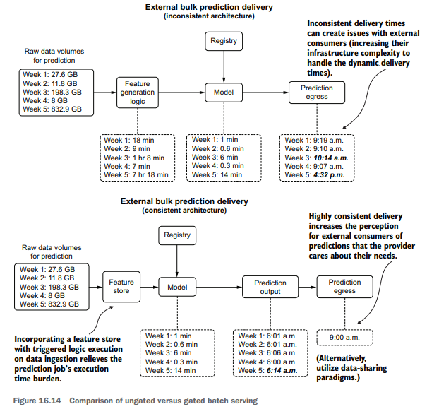
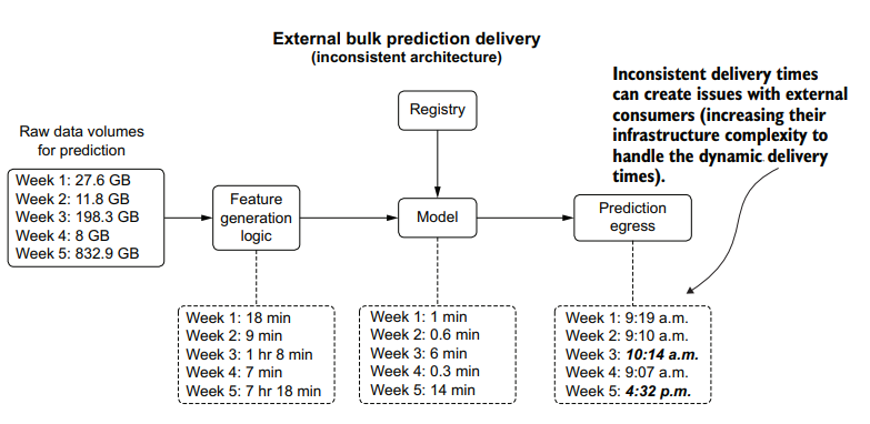
The one thing that does change with providing bulk predictions to an outside organization (generally applicable to business-to-business companies) when compared to other serving paradigms is in the timeliness of the delivery. While it may be obvious that a failure to deliver an extract of bulk predictions entirely is a bad thing, an inconsistent delivery can be just as detrimental. There is a simple solution to this, however, illustrated in the bottom portion of figure 16.14.

Figure 16.14 shows the comparison of gated and ungated serving to an external user group. By controlling a final-stage egress from the stored predictions in a scheduled batch prediction job, as well as coupling feature-generation logic to an ETL process governed by a feature store, delivery consistency from a chronological perspective can be guaranteed. While this may not seem an important consideration from the DS perspective of the team generating the predictions, having a predictable dataavailability schedule can dramatically increase the perceived professionalism of the serving company.

计算机代写|机器学习代写machine learning代考|QUALITY ASSURANCE

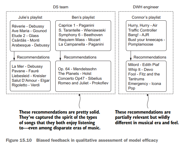
An occasionally overlooked aspect of serving bulk predictions externally (external to the DS and analytics groups at a company) is ensuring that a thorough quality check is performed on those predictions.

An internal project may rely on a simple check for overt prediction failures (for example, silent failures are ignored that result in null values, or a linear model predicts infinity). When sending data products externally, additional steps should be done to minimize the chances of end users of predictions finding fault with them. Since we, as humans, are so adept at finding abnormalities in patterns, a few scant issues in a batch-delivered prediction dataset can easily draw the focus of a consumer of the data, deteriorating their faith in the efficacy of the solution to the point of disuse.

In my experience, when delivering bulk predictions external to a team of data specialists, I’ve found it worthwhile to perform a few checks before releasing the data:

  • Validate the predictions against the training data:
  • Classification problems-Comparing aggregated class counts
  • Regression problems-Comparing prediction distribution
  • Unsupervised problems-Evaluating group membership counts
  • Check for prediction outliers (applicable to regression problems).
  • Build (if applicable) heuristics rules based on knowledge from SMEs to ensure that predictions are not outside the realm of possibility for the topic.
  • Validate incoming features (particularly encoded ones that may use a generic catchall encoding if the encoding key is previously unseen) to ensure that the data is fully compatible with the model as it was trained.

By running a few extra validation steps on the output of a batch prediction, a great deal of confusion and potential lessening of trust in the final product can be avoided in the eyes of end users.

计算机代写|机器学习代写machine learning代考|COMP4318

机器学习代考

计算机代写|机器学习代写machine learning代考|Bulk external delivery

批量外部交付的考虑因素与数据库或数据仓库的内部使用没有本质上的区别。这些服务案例之间唯一的实质性区别在于交付时间和预测监控方面。
交付的一致性
将结果批量交付给外部方与任何其他ML解决方案具有相同的相关性要求。无论您是在为内部团队构建某些东西,还是生成面向最终用户-客户的预测,创建有用预测的目标都不会改变。

与其他服务范式相比,向外部组织提供批量预测(通常适用于b2b公司)确实改变了一件事,那就是交付的及时性。虽然很明显,不能完全交付批量预测的摘要是一件坏事,但不一致的交付可能同样有害。但是,有一个简单的解决方案,如图16.14的底部部分所示。

图16.14显示了为外部用户组服务的门控和不门控的比较。通过控制计划批处理预测作业中存储的预测的最后阶段出口,以及将特征生成逻辑耦合到由特征存储管理的ETL过程,可以保证从时间顺序角度来看交付的一致性。虽然从生成预测的团队的DS角度来看,这似乎不是一个重要的考虑因素,但拥有可预测的数据可用性时间表可以显著提高服务公司的专业水平。

计算机代写|机器学习代写machine learning代考|QUALITY ASSURANCE

在向外部(公司的DS和分析组外部)提供批量预测时,一个偶尔被忽视的方面是确保对这些预测执行彻底的质量检查。

内部项目可能依赖于对公开预测失败的简单检查(例如,忽略导致空值的静默失败,或者线性模型预测无穷大)。在向外部发送数据产品时,应该采取额外的步骤,以尽量减少预测的最终用户发现错误的可能性。作为人类,我们非常善于发现模式中的异常,因此批量交付的预测数据集中的一些小问题很容易吸引数据消费者的注意力,从而降低他们对解决方案有效性的信心,直至不再使用。

根据我的经验,当向数据专家团队外部交付批量预测时,我发现在发布数据之前执行一些检查是值得的:

根据训练数据验证预测:

分类问题——比较聚合类计数

回归问题-比较预测分布

不受监督的问题——评估团队成员数量

检查预测异常值(适用于回归问题)。

基于中小企业的知识构建启发式规则(如果适用),以确保预测不会超出主题的可能性范围。

验证传入的特性(特别是编码的特性,如果编码键以前未见过,则可能使用通用的通用编码),以确保数据在训练时与模型完全兼容。

通过在批预测的输出上运行一些额外的验证步骤,可以避免在最终用户眼中对最终产品的大量混淆和潜在的信任度降低。

计算机代写|机器学习代写machine learning代考 请认准statistics-lab™

统计代写请认准statistics-lab™. statistics-lab™为您的留学生涯保驾护航。

金融工程代写

金融工程是使用数学技术来解决金融问题。金融工程使用计算机科学、统计学、经济学和应用数学领域的工具和知识来解决当前的金融问题,以及设计新的和创新的金融产品。

非参数统计代写

非参数统计指的是一种统计方法,其中不假设数据来自于由少数参数决定的规定模型;这种模型的例子包括正态分布模型和线性回归模型。

广义线性模型代考

广义线性模型(GLM)归属统计学领域,是一种应用灵活的线性回归模型。该模型允许因变量的偏差分布有除了正态分布之外的其它分布。

术语 广义线性模型(GLM)通常是指给定连续和/或分类预测因素的连续响应变量的常规线性回归模型。它包括多元线性回归,以及方差分析和方差分析(仅含固定效应)。

有限元方法代写

有限元方法(FEM)是一种流行的方法,用于数值解决工程和数学建模中出现的微分方程。典型的问题领域包括结构分析、传热、流体流动、质量运输和电磁势等传统领域。

有限元是一种通用的数值方法,用于解决两个或三个空间变量的偏微分方程(即一些边界值问题)。为了解决一个问题,有限元将一个大系统细分为更小、更简单的部分,称为有限元。这是通过在空间维度上的特定空间离散化来实现的,它是通过构建对象的网格来实现的:用于求解的数值域,它有有限数量的点。边界值问题的有限元方法表述最终导致一个代数方程组。该方法在域上对未知函数进行逼近。[1] 然后将模拟这些有限元的简单方程组合成一个更大的方程系统,以模拟整个问题。然后,有限元通过变化微积分使相关的误差函数最小化来逼近一个解决方案。

tatistics-lab作为专业的留学生服务机构,多年来已为美国、英国、加拿大、澳洲等留学热门地的学生提供专业的学术服务,包括但不限于Essay代写,Assignment代写,Dissertation代写,Report代写,小组作业代写,Proposal代写,Paper代写,Presentation代写,计算机作业代写,论文修改和润色,网课代做,exam代考等等。写作范围涵盖高中,本科,研究生等海外留学全阶段,辐射金融,经济学,会计学,审计学,管理学等全球99%专业科目。写作团队既有专业英语母语作者,也有海外名校硕博留学生,每位写作老师都拥有过硬的语言能力,专业的学科背景和学术写作经验。我们承诺100%原创,100%专业,100%准时,100%满意。

随机分析代写


随机微积分是数学的一个分支,对随机过程进行操作。它允许为随机过程的积分定义一个关于随机过程的一致的积分理论。这个领域是由日本数学家伊藤清在第二次世界大战期间创建并开始的。

时间序列分析代写

随机过程,是依赖于参数的一组随机变量的全体,参数通常是时间。 随机变量是随机现象的数量表现,其时间序列是一组按照时间发生先后顺序进行排列的数据点序列。通常一组时间序列的时间间隔为一恒定值(如1秒,5分钟,12小时,7天,1年),因此时间序列可以作为离散时间数据进行分析处理。研究时间序列数据的意义在于现实中,往往需要研究某个事物其随时间发展变化的规律。这就需要通过研究该事物过去发展的历史记录,以得到其自身发展的规律。

回归分析代写

多元回归分析渐进(Multiple Regression Analysis Asymptotics)属于计量经济学领域,主要是一种数学上的统计分析方法,可以分析复杂情况下各影响因素的数学关系,在自然科学、社会和经济学等多个领域内应用广泛。

MATLAB代写

MATLAB 是一种用于技术计算的高性能语言。它将计算、可视化和编程集成在一个易于使用的环境中,其中问题和解决方案以熟悉的数学符号表示。典型用途包括:数学和计算算法开发建模、仿真和原型制作数据分析、探索和可视化科学和工程图形应用程序开发,包括图形用户界面构建MATLAB 是一个交互式系统,其基本数据元素是一个不需要维度的数组。这使您可以解决许多技术计算问题,尤其是那些具有矩阵和向量公式的问题,而只需用 C 或 Fortran 等标量非交互式语言编写程序所需的时间的一小部分。MATLAB 名称代表矩阵实验室。MATLAB 最初的编写目的是提供对由 LINPACK 和 EISPACK 项目开发的矩阵软件的轻松访问,这两个项目共同代表了矩阵计算软件的最新技术。MATLAB 经过多年的发展,得到了许多用户的投入。在大学环境中,它是数学、工程和科学入门和高级课程的标准教学工具。在工业领域,MATLAB 是高效研究、开发和分析的首选工具。MATLAB 具有一系列称为工具箱的特定于应用程序的解决方案。对于大多数 MATLAB 用户来说非常重要,工具箱允许您学习应用专业技术。工具箱是 MATLAB 函数(M 文件)的综合集合,可扩展 MATLAB 环境以解决特定类别的问题。可用工具箱的领域包括信号处理、控制系统、神经网络、模糊逻辑、小波、仿真等。

R语言代写问卷设计与分析代写
PYTHON代写回归分析与线性模型代写
MATLAB代写方差分析与试验设计代写
STATA代写机器学习/统计学习代写
SPSS代写计量经济学代写
EVIEWS代写时间序列分析代写
EXCEL代写深度学习代写
SQL代写各种数据建模与可视化代写

计算机代写|深度学习代写deep learning代考|T81-558

如果你也在 怎样代写深度学习Deep Learning 这个学科遇到相关的难题,请随时右上角联系我们的24/7代写客服。深度学习Deep Learning(是机器学习的一种,也是人工智能的一种方法。通过用简单的世界来构建复杂的世界表示,深度学习技术在计算机视觉、语音识别、自然语言处理、临床应用和其他领域取得了最先进的成果——有望(也有可能)改变社会。

深度学习Deep Learning架构,如深度神经网络、深度信念网络、深度强化学习、递归神经网络、卷积神经网络和变形金刚,已被应用于包括计算机视觉、语音识别、自然语言处理、机器翻译、生物信息学、药物设计、医学图像分析、气候科学、材料检测和棋盘游戏程序等领域,它们产生的结果与人类专家的表现相当,在某些情况下甚至超过了人类专家。

statistics-lab™ 为您的留学生涯保驾护航 在代写深度学习deep learning方面已经树立了自己的口碑, 保证靠谱, 高质且原创的统计Statistics代写服务。我们的专家在代写深度学习deep learning代写方面经验极为丰富,各种代写深度学习deep learning相关的作业也就用不着说。

计算机代写|深度学习代写deep learning代考|T81-558

计算机代写|深度学习代写deep learning代考|Criteria of Adequacy

To summarize, a satisfactory explanation for cognitive change consists of at least the following components:

  1. A description of the explanatory target itself. The latter can be a unique learning event, a particular change that happened for a person at some point in time and place, a type of change (belief revision) or a recurring pattern of change (the learning curve).
  2. A background theory of the relevant aspect or aspects of the cognitive architecture. It will include a specification of the types of mental representations assumed; the repertoire of basic cognitive processes that create, manipulate and utilize these representations; and the mechanism that passes control among those processes. This background theory serves as a processing context within which the postulated change mechanisms are assumed to operate.
  3. A repertoire of learning mechanisms. The change produced by a learning mechanism is typically small in scope compared to the explanatory target. The micro-theories proposed in this book distinguish mechanisms for monotonic learning from mechanisms for non-monotonic learning.
  4. A specification of the triggering conditions under which each learning mechanism tends to occur.
  1. An articulation of the mechanisms and the triggering conditions vis-à-vis the explanatory target. An explanation is a demonstration that (a) the relevant triggering conditions held in the situation in which the target change is supposed to have happened, and (b) the specified learning mechanisms, if triggered under those conditions, would in fact produce the observed change. If the explanatory target is a pattern of change, then the articulation needs to show why that type of change tends to recur.
  2. An explanation is the more satisfactory if it comes with an argument to the effect that the postulated change mechanisms scale up, that is, produce observed or plausible outcomes over long periods of time and across system levels.
  3. Last, but not least, an explanation is more satisfactory if it comes with a demonstration that the postulated learning mechanisms can support successful practice.

In the terminology of the philosophy of science, these seven points are criteria of adequacy. Their satisfaction does not guarantee the truth of a theory. They constitute a test that a purported explanation has to pass in order to be a viable candidate. Bluntly put: If a theory or hypothesis lacks these features, it is not worth considering.

计算机代写|深度学习代写deep learning代考|THE PATH AHEAD

The research strategy behind the investigations reported in this book is to study specific types of non-monotonic change and propose micro-theories to explain them. Once the micro-theories have been clearly formulated, they can be mined for deeper principles, if any. In this approach, theory construction does not proceed in an inductive, bottom-up or top-down fashion. The choice of phenomena to be studied is guided by the prior decision to focus on non-monotonic change, itself a theoretical concept. On the other hand, theory construction does not proceed by pushing a single concept or principle into every corner and crevasse of the cognitive landscape. Instead, the principles of each micro-theory are designed to provide understanding of the case that inspires them without regard for their applicability elsewhere. The deeper theory, if any, is to emerge from the conceptual analysis of the micro-theories. In this layered approach, the degree of unification to be sought is itself an outcome of the investigation rather than something given at the outset. Figure 2.3 shows the overall structure of the enterprise.

Following this strategy, Parts II-IV investigate three cases of nonmonotonic change: the creation of novelty, adaptation to an unfamiliar or changing task environment, and conversion from one belief system to another.

The factor that unites these three types of cognitive change is that they require the learner to overcome some part of his prior knowledge, the distinctive feature of non-monotonic learning. They are separated by the key phenomena, the learning scenarios and experimental paradigms in which we can observe those phenomena and the intellectual traditions within which past explanations for those phenomena have been embedded.

Parts II and III consist of three chapters each. The first chapter in each part frames the theoretical problem to be solved, anchoring it in everyday experience as well as in prior research. The latter includes any work that addresses the relevant problem, regardless of age or disciplinary label. In the second chapter, I state a micro-theory for the relevant explanatory target. In the third chapter, I develop the broader implications of the micro-theory, especially in regard to its interactions with other processes, the accumulation of changes over time and the projection of its effects across system levels. Part IV follows the same schema, except that the third chapter is absent.

计算机代写|深度学习代写deep learning代考|T81-558

深度学习代写

计算机代写|深度学习代写deep learning代考|Criteria of Adequacy

总而言之,对认知变化的一个令人满意的解释至少包括以下几个部分:

对解释对象本身的描述。后者可以是一个独特的学习事件,一个人在某个时间和地点发生的特定变化,一种变化(信念修正)或反复出现的变化模式(学习曲线)。

认知体系的相关方面或方面的背景理论。它将包括对假定的心理表征类型的说明;创造、操纵和利用这些表征的基本认知过程;以及在这些过程之间传递控制的机制。这个背景理论作为一个处理环境,在这个环境中,假设的变化机制被假设运作。

一整套学习机制。与解释目标相比,学习机制产生的变化通常是很小的。本书提出的微观理论区分了单调学习机制和非单调学习机制。

每种学习机制发生的触发条件的说明。

对-à-vis解释目标的机制和触发条件的阐述。解释是证明(a)在目标变化发生的情境中存在相关触发条件,以及(b)在这些条件下触发的特定学习机制实际上会产生观察到的变化。如果解释性目标是一种变化模式,那么表述需要显示为什么这种类型的变化倾向于重复出现。

如果一个解释带有这样的论点,即假设的变化机制按比例扩大,也就是说,在很长一段时间内和跨系统级别产生可观察到的或似是而非的结果,那么这个解释就更令人满意。

最后,但并非最不重要的是,如果一个解释能够证明假设的学习机制能够支持成功的实践,那么这个解释就会更令人满意。

用科学哲学的术语来说,这七点就是充分性的标准。他们的满意并不能保证理论的真实性。它们构成了一种测试,一个声称的解释必须通过这个测试才能成为一个可行的候选者。坦率地说:如果一个理论或假设缺乏这些特征,它就不值得考虑。

计算机代写|深度学习代写deep learning代考|THE PATH AHEAD

本书中报告的调查背后的研究策略是研究特定类型的非单调变化,并提出微观理论来解释它们。一旦微观理论被清晰地表述出来,它们就可以被挖掘出更深层次的原理,如果有的话。在这种方法中,理论构建不是以归纳、自下而上或自上而下的方式进行的。要研究的现象的选择是由先前决定关注非单调变化指导的,非单调变化本身就是一个理论概念。另一方面,理论建设不是将单一的概念或原则推到认知景观的每一个角落和裂缝中。相反,每一种微观理论的原则都旨在提供对激发它们的案例的理解,而不考虑它们在其他地方的适用性。更深层次的理论,如果有的话,是从微观理论的概念分析中产生的。在这种分层的方法中,要寻求的统一程度本身就是调查的结果,而不是一开始就给出的东西。企业整体结构如图2.3所示。

根据这一策略,第二至第四部分研究了三种非单调变化的情况:创造新颖性,适应不熟悉或不断变化的任务环境,以及从一种信仰体系转变为另一种信仰体系。

将这三种类型的认知变化联系在一起的因素是,它们都要求学习者克服其先前知识的某些部分,这是非单调学习的显著特征。它们被关键现象、学习场景和实验范式分开,我们可以在这些现象中观察到这些现象,以及过去对这些现象的解释所包含的知识传统。

第二部分和第三部分各由三章组成。每个部分的第一章都是要解决的理论问题,将其固定在日常经验和先前的研究中。后者包括任何解决相关问题的工作,无论年龄或学科标签如何。在第二章中,我为相关的解释对象阐述了一个微观理论。在第三章中,我发展了微观理论的更广泛的含义,特别是关于它与其他过程的相互作用,随时间变化的积累以及它在系统水平上的影响的预测。第四部分遵循同样的模式,只是没有第三章。

计算机代写|深度学习代写deep learning代考 请认准statistics-lab™

统计代写请认准statistics-lab™. statistics-lab™为您的留学生涯保驾护航。

金融工程代写

金融工程是使用数学技术来解决金融问题。金融工程使用计算机科学、统计学、经济学和应用数学领域的工具和知识来解决当前的金融问题,以及设计新的和创新的金融产品。

非参数统计代写

非参数统计指的是一种统计方法,其中不假设数据来自于由少数参数决定的规定模型;这种模型的例子包括正态分布模型和线性回归模型。

广义线性模型代考

广义线性模型(GLM)归属统计学领域,是一种应用灵活的线性回归模型。该模型允许因变量的偏差分布有除了正态分布之外的其它分布。

术语 广义线性模型(GLM)通常是指给定连续和/或分类预测因素的连续响应变量的常规线性回归模型。它包括多元线性回归,以及方差分析和方差分析(仅含固定效应)。

有限元方法代写

有限元方法(FEM)是一种流行的方法,用于数值解决工程和数学建模中出现的微分方程。典型的问题领域包括结构分析、传热、流体流动、质量运输和电磁势等传统领域。

有限元是一种通用的数值方法,用于解决两个或三个空间变量的偏微分方程(即一些边界值问题)。为了解决一个问题,有限元将一个大系统细分为更小、更简单的部分,称为有限元。这是通过在空间维度上的特定空间离散化来实现的,它是通过构建对象的网格来实现的:用于求解的数值域,它有有限数量的点。边界值问题的有限元方法表述最终导致一个代数方程组。该方法在域上对未知函数进行逼近。[1] 然后将模拟这些有限元的简单方程组合成一个更大的方程系统,以模拟整个问题。然后,有限元通过变化微积分使相关的误差函数最小化来逼近一个解决方案。

tatistics-lab作为专业的留学生服务机构,多年来已为美国、英国、加拿大、澳洲等留学热门地的学生提供专业的学术服务,包括但不限于Essay代写,Assignment代写,Dissertation代写,Report代写,小组作业代写,Proposal代写,Paper代写,Presentation代写,计算机作业代写,论文修改和润色,网课代做,exam代考等等。写作范围涵盖高中,本科,研究生等海外留学全阶段,辐射金融,经济学,会计学,审计学,管理学等全球99%专业科目。写作团队既有专业英语母语作者,也有海外名校硕博留学生,每位写作老师都拥有过硬的语言能力,专业的学科背景和学术写作经验。我们承诺100%原创,100%专业,100%准时,100%满意。

随机分析代写


随机微积分是数学的一个分支,对随机过程进行操作。它允许为随机过程的积分定义一个关于随机过程的一致的积分理论。这个领域是由日本数学家伊藤清在第二次世界大战期间创建并开始的。

时间序列分析代写

随机过程,是依赖于参数的一组随机变量的全体,参数通常是时间。 随机变量是随机现象的数量表现,其时间序列是一组按照时间发生先后顺序进行排列的数据点序列。通常一组时间序列的时间间隔为一恒定值(如1秒,5分钟,12小时,7天,1年),因此时间序列可以作为离散时间数据进行分析处理。研究时间序列数据的意义在于现实中,往往需要研究某个事物其随时间发展变化的规律。这就需要通过研究该事物过去发展的历史记录,以得到其自身发展的规律。

回归分析代写

多元回归分析渐进(Multiple Regression Analysis Asymptotics)属于计量经济学领域,主要是一种数学上的统计分析方法,可以分析复杂情况下各影响因素的数学关系,在自然科学、社会和经济学等多个领域内应用广泛。

MATLAB代写

MATLAB 是一种用于技术计算的高性能语言。它将计算、可视化和编程集成在一个易于使用的环境中,其中问题和解决方案以熟悉的数学符号表示。典型用途包括:数学和计算算法开发建模、仿真和原型制作数据分析、探索和可视化科学和工程图形应用程序开发,包括图形用户界面构建MATLAB 是一个交互式系统,其基本数据元素是一个不需要维度的数组。这使您可以解决许多技术计算问题,尤其是那些具有矩阵和向量公式的问题,而只需用 C 或 Fortran 等标量非交互式语言编写程序所需的时间的一小部分。MATLAB 名称代表矩阵实验室。MATLAB 最初的编写目的是提供对由 LINPACK 和 EISPACK 项目开发的矩阵软件的轻松访问,这两个项目共同代表了矩阵计算软件的最新技术。MATLAB 经过多年的发展,得到了许多用户的投入。在大学环境中,它是数学、工程和科学入门和高级课程的标准教学工具。在工业领域,MATLAB 是高效研究、开发和分析的首选工具。MATLAB 具有一系列称为工具箱的特定于应用程序的解决方案。对于大多数 MATLAB 用户来说非常重要,工具箱允许您学习应用专业技术。工具箱是 MATLAB 函数(M 文件)的综合集合,可扩展 MATLAB 环境以解决特定类别的问题。可用工具箱的领域包括信号处理、控制系统、神经网络、模糊逻辑、小波、仿真等。

R语言代写问卷设计与分析代写
PYTHON代写回归分析与线性模型代写
MATLAB代写方差分析与试验设计代写
STATA代写机器学习/统计学习代写
SPSS代写计量经济学代写
EVIEWS代写时间序列分析代写
EXCEL代写深度学习代写
SQL代写各种数据建模与可视化代写

计算机代写|深度学习代写deep learning代考|CS7643

如果你也在 怎样代写深度学习Deep Learning 这个学科遇到相关的难题,请随时右上角联系我们的24/7代写客服。深度学习Deep Learning(是机器学习的一种,也是人工智能的一种方法。通过用简单的世界来构建复杂的世界表示,深度学习技术在计算机视觉、语音识别、自然语言处理、临床应用和其他领域取得了最先进的成果——有望(也有可能)改变社会。

深度学习Deep Learning架构,如深度神经网络、深度信念网络、深度强化学习、递归神经网络、卷积神经网络和变形金刚,已被应用于包括计算机视觉、语音识别、自然语言处理、机器翻译、生物信息学、药物设计、医学图像分析、气候科学、材料检测和棋盘游戏程序等领域,它们产生的结果与人类专家的表现相当,在某些情况下甚至超过了人类专家。

statistics-lab™ 为您的留学生涯保驾护航 在代写深度学习deep learning方面已经树立了自己的口碑, 保证靠谱, 高质且原创的统计Statistics代写服务。我们的专家在代写深度学习deep learning代写方面经验极为丰富,各种代写深度学习deep learning相关的作业也就用不着说。

计算机代写|深度学习代写deep learning代考|CS7643

计算机代写|深度学习代写deep learning代考|EXPLAINING CHANGE

If the mind is a system for processing knowledge representations in the service of action and discourse, how does it change over time? What form should an explanation for cognitive change take? What are the criteria of a satisfactory explanation and what issues arise in the construction of such explanations? It is informative to consider successful explanations for other types of change. Cognitive psychologists need not imitate other sciences or assume that their own theories must, in the end, look like those of any other science, but neither is it wise to assume that other sciences have no lessons to teach. Natural scientists, social scientists and humanists have grappled with the concept of change and their successes provide calories for psychological thought.
Componential Explanations
To extract the general features of scientific explanations of change, consider contagion and electrolysis, two seemingly different phenomena. How do contagious diseases like yellow fever spread such that we suffer epidemics ${ }^{28}$ It required considerable research to identify all parts of this complicated process. Although a specialist on yellow fever could add innumerable details, a mere outline suffices here: The disease is caused by a germ that multiplies in a person’s body, causing the symptoms. The sick person is bitten by a mosquito, which sucks up blood that contains the germ. The mosquito flies to another person and bites again, at which point some of the germs are inserted in that person’s body and begin to multiply there; and so on. This narrative makes understandable several otherwise inexplicable aspects of yellow fever, such as the timing and geographical location of epidemics and the pattern of diffusion within each epidemic.

Consider next the explanation for the electrolysis of water: Pass electricity through water and the water turns into hydrogen and oxygen gases. ${ }^{39}$ How does this chemical transformation happen? As every chemistry student knows, water molecules consist of two hydrogen atoms and one oxygen atom connected via co-valent bonds, $\mathrm{H}_2 \mathrm{O}$ in the standard chemical formula. The electrical current dissolves the bonds, causing the hydrogen and oxygen atoms to drift apart. When two hydrogen atoms bump into each other, they bind, forming one molecule of hydrogen $\left(\mathrm{H}_2\right)$. Likewise, two oxygen atoms bind to form one molecule of oxygen $\left(\mathrm{O}_2\right)$. So two water molecules turn into two hydrogen molecules and one molecule of oxygen.

计算机代写|深度学习代写deep learning代考|The Repertoire of Learning Mechanisms

Sciences differ in an interesting way with respect to their repertoires of unit changes. Some fields of research attribute all their phenomena to a single type of change. ${ }^{42}$ Adherents of the mechanical world view in the 17 th and 18 th centuries tried to explain all of physics through the motions of physical bodies and the forces they exert on each other. Chemists explain all chemical reactions in terms of the rearrangement of atoms through the breaking and forming of atomic bonds. Earth scientists, in contrast, draw upon a rich and varied repertoire of change mechanisms: glaciation in response to astronomical cycles, plate tectonics, erosion caused by water freezing in cracks, the actions of wind and water on soil and sand and so on. ${ }^{43}$ Whether a science will turn out to need a sparse or a rich repertoire of change mechanisms cannot be known ahead of investigation.
Tradition has handed down a long list of suggestions about the basic processes of knowledge change. I refer to them as learning mechanisms. Perhaps association, the idea that knowledge changes by the creation of a link between two previously unconnected ideas or concepts, is the oldest learning mechanism of all. The notion of generalization (abstraction, induction) – the idea that the mind extracts commonalities from sets of instances – has likewise been with us since antiquity. Over time, psychologists have coined a wide variety of terms to refer to what are ostensibly different types of cognitive change: association, automatization, belief revision, categorization, chunking, conceptual change, concept learning, conditioning, cognitive development, discrimination, equilibration, generalization, habit formation, implicit learning, maturation, memorization, perceptual learning, induction, knowledge acquisition, list learning, skill acquisition, schema extraction, stage transition, strategy change and theory change.
This plethora of technical terms implicitly claims that cognitive change is a heterogeneous phenomenon and intuition provides some support. It is certainly plausible that, for example, conceptual knowledge and skills are acquired via different mechanisms. Furthermore, knowledge can change both by becoming more abstract and by becoming more specific, two processes that are each others’ opposites and hence difficult to explain with a single mechanism. We should not expect a final theory of learning to pull together all of cognitive change in a single law of learning to take its place next to Isaac Newton’s law of gravitation as one of the triumphs of science.

计算机代写|深度学习代写deep learning代考|CS7643

深度学习代写

计算机代写|深度学习代写deep learning代考|EXPLAINING CHANGE

如果心灵是一个为行为和话语服务而处理知识表征的系统,那么它是如何随时间变化的呢?对认知变化的解释应该采取什么形式?一个令人满意的解释的标准是什么?在构建这样的解释时会出现什么问题?考虑对其他类型的变化的成功解释是有益的。认知心理学家不需要模仿其他科学,也不需要假设他们自己的理论最终必须与任何其他科学的理论一样,但假设其他科学没有教训可教也是不明智的。自然科学家、社会科学家和人文主义者一直在努力研究变化的概念,他们的成功为心理学思想提供了热量。
成分的解释
为了提取变化的科学解释的一般特征,考虑传染和电解这两种看似不同的现象。像黄热病这样的传染病是如何传播的,使我们遭受流行病的折磨?{}^{28}$需要进行大量的研究,以确定这一复杂过程的所有部分。虽然黄热病专家可以提供无数的细节,但在这里只做一个概述就足够了:这种疾病是由一种在人体内繁殖的细菌引起的,从而引起症状。病人被蚊子叮咬,蚊子会吸出含有细菌的血液。蚊子飞到另一个人身上并再次叮咬,这时一些细菌被插入那个人的身体并开始在那里繁殖;等等……这种叙述使人们能够理解黄热病的一些其他方面无法解释的问题,例如流行病的时间和地理位置以及每次流行病的传播模式。

接下来考虑一下对水的电解的解释:把电通过水,水就会变成氢气和氧气。${}^{39}$这种化学转变是如何发生的?每个学化学的学生都知道,水分子是由两个氢原子和一个氧原子通过共价键连接而成的,在标准化学式中是$\ mathm {H}_2 \ mathm {O}$。电流溶解了化学键,导致氢原子和氧原子漂移。当两个氢原子相互碰撞时,它们结合,形成一个氢分子$\左(\ mathm {H}_2\右)$。同样,两个氧原子结合形成一个氧分子$\left(\ mathm {O}_2\right)$。所以两个水分子变成了两个氢分子和一个氧分子。

计算机代写|深度学习代写deep learning代考|The Repertoire of Learning Mechanisms

科学以一种有趣的方式不同于它们对单位变化的反应。一些研究领域把所有的现象都归结为一种变化。17世纪和18世纪机械世界观的拥护者试图通过物理物体的运动和它们相互施加的力来解释所有的物理学。化学家用原子键断裂和形成的原子重排来解释所有的化学反应。相比之下,地球科学家则利用了丰富多样的变化机制:与天文周期有关的冰川作用、板块构造、由裂缝中的水冻结引起的侵蚀、风和水对土壤和沙子的作用等等。${}^{43}$一门科学最终需要的变化机制是稀疏的还是丰富的,在调查之前是不可能知道的。
传统已经流传了一长串关于知识变化的基本过程的建议。我把它们称为学习机制。也许联想是所有学习机制中最古老的。联想是指知识通过在两个先前不相关的想法或概念之间建立联系而发生变化。概括(抽象、归纳)的概念——即思维从一系列实例中提取共性的观点——同样自古以来就与我们同在。随着时间的推移,心理学家创造了各种各样的术语来指代表面上不同类型的认知变化:联想、自动化、信念修正、分类、分块、概念变化、概念学习、条件反射、认知发展、辨别、平衡、概括、习惯形成、内隐学习、成熟、记忆、感知学习、归纳、知识获取、列表学习、技能获取、图式提取、阶段转换、策略变化和理论变化。
这些过多的技术术语暗示了认知变化是一种异质现象,直觉提供了一些支持。例如,概念性知识和技能是通过不同的机制获得的,这当然是合理的。此外,知识可以通过变得更抽象和更具体来改变,这两个过程是彼此对立的,因此很难用单一机制来解释。我们不应该期望一个最终的学习理论将所有的认知变化集中在一个单一的学习定律中,以取代艾萨克·牛顿的万有引力定律,成为科学的胜利之一。

计算机代写|深度学习代写deep learning代考 请认准statistics-lab™

统计代写请认准statistics-lab™. statistics-lab™为您的留学生涯保驾护航。

金融工程代写

金融工程是使用数学技术来解决金融问题。金融工程使用计算机科学、统计学、经济学和应用数学领域的工具和知识来解决当前的金融问题,以及设计新的和创新的金融产品。

非参数统计代写

非参数统计指的是一种统计方法,其中不假设数据来自于由少数参数决定的规定模型;这种模型的例子包括正态分布模型和线性回归模型。

广义线性模型代考

广义线性模型(GLM)归属统计学领域,是一种应用灵活的线性回归模型。该模型允许因变量的偏差分布有除了正态分布之外的其它分布。

术语 广义线性模型(GLM)通常是指给定连续和/或分类预测因素的连续响应变量的常规线性回归模型。它包括多元线性回归,以及方差分析和方差分析(仅含固定效应)。

有限元方法代写

有限元方法(FEM)是一种流行的方法,用于数值解决工程和数学建模中出现的微分方程。典型的问题领域包括结构分析、传热、流体流动、质量运输和电磁势等传统领域。

有限元是一种通用的数值方法,用于解决两个或三个空间变量的偏微分方程(即一些边界值问题)。为了解决一个问题,有限元将一个大系统细分为更小、更简单的部分,称为有限元。这是通过在空间维度上的特定空间离散化来实现的,它是通过构建对象的网格来实现的:用于求解的数值域,它有有限数量的点。边界值问题的有限元方法表述最终导致一个代数方程组。该方法在域上对未知函数进行逼近。[1] 然后将模拟这些有限元的简单方程组合成一个更大的方程系统,以模拟整个问题。然后,有限元通过变化微积分使相关的误差函数最小化来逼近一个解决方案。

tatistics-lab作为专业的留学生服务机构,多年来已为美国、英国、加拿大、澳洲等留学热门地的学生提供专业的学术服务,包括但不限于Essay代写,Assignment代写,Dissertation代写,Report代写,小组作业代写,Proposal代写,Paper代写,Presentation代写,计算机作业代写,论文修改和润色,网课代做,exam代考等等。写作范围涵盖高中,本科,研究生等海外留学全阶段,辐射金融,经济学,会计学,审计学,管理学等全球99%专业科目。写作团队既有专业英语母语作者,也有海外名校硕博留学生,每位写作老师都拥有过硬的语言能力,专业的学科背景和学术写作经验。我们承诺100%原创,100%专业,100%准时,100%满意。

随机分析代写


随机微积分是数学的一个分支,对随机过程进行操作。它允许为随机过程的积分定义一个关于随机过程的一致的积分理论。这个领域是由日本数学家伊藤清在第二次世界大战期间创建并开始的。

时间序列分析代写

随机过程,是依赖于参数的一组随机变量的全体,参数通常是时间。 随机变量是随机现象的数量表现,其时间序列是一组按照时间发生先后顺序进行排列的数据点序列。通常一组时间序列的时间间隔为一恒定值(如1秒,5分钟,12小时,7天,1年),因此时间序列可以作为离散时间数据进行分析处理。研究时间序列数据的意义在于现实中,往往需要研究某个事物其随时间发展变化的规律。这就需要通过研究该事物过去发展的历史记录,以得到其自身发展的规律。

回归分析代写

多元回归分析渐进(Multiple Regression Analysis Asymptotics)属于计量经济学领域,主要是一种数学上的统计分析方法,可以分析复杂情况下各影响因素的数学关系,在自然科学、社会和经济学等多个领域内应用广泛。

MATLAB代写

MATLAB 是一种用于技术计算的高性能语言。它将计算、可视化和编程集成在一个易于使用的环境中,其中问题和解决方案以熟悉的数学符号表示。典型用途包括:数学和计算算法开发建模、仿真和原型制作数据分析、探索和可视化科学和工程图形应用程序开发,包括图形用户界面构建MATLAB 是一个交互式系统,其基本数据元素是一个不需要维度的数组。这使您可以解决许多技术计算问题,尤其是那些具有矩阵和向量公式的问题,而只需用 C 或 Fortran 等标量非交互式语言编写程序所需的时间的一小部分。MATLAB 名称代表矩阵实验室。MATLAB 最初的编写目的是提供对由 LINPACK 和 EISPACK 项目开发的矩阵软件的轻松访问,这两个项目共同代表了矩阵计算软件的最新技术。MATLAB 经过多年的发展,得到了许多用户的投入。在大学环境中,它是数学、工程和科学入门和高级课程的标准教学工具。在工业领域,MATLAB 是高效研究、开发和分析的首选工具。MATLAB 具有一系列称为工具箱的特定于应用程序的解决方案。对于大多数 MATLAB 用户来说非常重要,工具箱允许您学习应用专业技术。工具箱是 MATLAB 函数(M 文件)的综合集合,可扩展 MATLAB 环境以解决特定类别的问题。可用工具箱的领域包括信号处理、控制系统、神经网络、模糊逻辑、小波、仿真等。

R语言代写问卷设计与分析代写
PYTHON代写回归分析与线性模型代写
MATLAB代写方差分析与试验设计代写
STATA代写机器学习/统计学习代写
SPSS代写计量经济学代写
EVIEWS代写时间序列分析代写
EXCEL代写深度学习代写
SQL代写各种数据建模与可视化代写

计算机代写|深度学习代写deep learning代考|CS230

如果你也在 怎样代写深度学习Deep Learning 这个学科遇到相关的难题,请随时右上角联系我们的24/7代写客服。深度学习Deep Learning(是机器学习的一种,也是人工智能的一种方法。通过用简单的世界来构建复杂的世界表示,深度学习技术在计算机视觉、语音识别、自然语言处理、临床应用和其他领域取得了最先进的成果——有望(也有可能)改变社会。

深度学习Deep Learning架构,如深度神经网络、深度信念网络、深度强化学习、递归神经网络、卷积神经网络和变形金刚,已被应用于包括计算机视觉、语音识别、自然语言处理、机器翻译、生物信息学、药物设计、医学图像分析、气候科学、材料检测和棋盘游戏程序等领域,它们产生的结果与人类专家的表现相当,在某些情况下甚至超过了人类专家。

statistics-lab™ 为您的留学生涯保驾护航 在代写深度学习deep learning方面已经树立了自己的口碑, 保证靠谱, 高质且原创的统计Statistics代写服务。我们的专家在代写深度学习deep learning代写方面经验极为丰富,各种代写深度学习deep learning相关的作业也就用不着说。

计算机代写|深度学习代写deep learning代考|CS230

计算机代写|深度学习代写deep learning代考|DEEP LEARNING

If prior experience is a seriously fallible guide, learning cannot consist solely or even primarily of accumulating experiences, finding regularities therein and projecting those regularities onto the future. To successfully deal with thoroughgoing change, human beings need the ability to override the imperatives of experience and consider actions other than those suggested by the projection of that experience onto the situation at hand. Given the turbulent character of reality, the evolutionary strategy of relying primarily on learned rather than innate behaviors drove the human species to evolve cognitive mechanisms that override prior experience. This is the main theme of this book, so it deserves a label and an explicit statement:
The Deep Learning Hypothesis
In the course of shifting the basis for action from innate structures to acquired knowledge and skills, human beings evolved cognitive processes and mechanisms that enable them to suppress their experience and override its imperatives for action.
The Deep Learning Hypothesis does not deny the existence of cognitive mechanisms that operate on the basis of experience. Inductive learning works in tight contexts and people obviously do possess the processes for encoding episodic information into memory, inductive reasoning, projection and planning that are described in cognitive psychology textbooks. The type of learning supported by those processes generates new knowledge that is consistent with what was known before. Borrowing a useful term from logicians, I refer to such additive cognitive growth as monotonic.

The claim of the Deep Learning Hypothesis is that monotonic learning is at most half the story. The other half describes how we abandon, override, reject, retract or suppress knowledge that we had previously accepted as valid in order to track a constantly shifting and fundamentally unpredictable environment and thereby indirectly create mental space for alternative or even contradictory concepts, beliefs, ideas and strategies. A complete theory of human learning must complement inductive mechanisms with a second set of non-monotonic learning mechanisms that allow experience to be overruled.
The hypothesis that we possess cognitive mechanisms for overriding the imperatives of the past does not imply that doing so is effortless. Everyday life requires a balance between projecting and overriding past experience – what philosopher Thomas S. Kuhn has called “the essential tension” – and there is no reason to believe that evolution provided us with a perfect solution to this balancing problem. ${ }^{53}$ To explain cognitive change is to explain both the possibility and difficulty of non-monotonic change.

计算机代写|深度学习代写deep learning代考|CLOSING THE ESCAPE ROUTES

Psychology is the science of mind. Nevertheless, some psychologists have tried to replace the task of describing how the mind works by the task of describing something else. Different schools of thought have proposed different replacements.
According to the phenomenological approach, to describe mind is to describe subjective experience; that is, to state what a person is consciously perceiving, feeling, remembering and thinking. ${ }^6$ Once the contents of consciousness have been described, there is yet more to say, but what is left to say falls within the scope of neuroscience. Phenomenologists do not deny mind but limit its scope. Psychology’s responsibilities end at the edge of consciousness; the rest is neurons.

The emphasis on subjective experience is useful. Cognitive processes are expressed in subjective experience as well as in action and discourse. For example, we are all familiar with the frustration of trying to recall a name or a fact that refuses to be recalled, the elation associated with a sudden insight into a recalcitrant problem and the satisfaction of performing a complex skill thoroughly mastered. If psychology is to be a tool for understanding ourselves, our theories must explain the flow of subjective experiences as well as the streams of action and discourse.

But basic facts about cognition reveal as fallacious the idea that the mind can be reduced to nothing but subjective experience. Consider trying to recall a name, failing to do so but spontaneously succeeding a short while later. There cannot be a phenomenological explanation of this type of cognitive event. The subjective experience consists of the effort to recall, the blank mind that accompanies failure to recall and the slight surprise and relief of tension that accompanies the subsequent success. But this remains a description, not an explanation. The process that produces these conscious experiences – retrieval from long-term memory – is not itself conscious. An account of the subjective experiences, no matter how accurate, does not suffice to explain the regularities associated with retrieval failures, tip-of-the-tongue feelings and similar mental events. ${ }^7$ This and many other observations force the conclusion that there are mental processes that are not conscious. The weakness of the phenomenological approach does not lie in its descriptions of conscious experiences but in the unwarranted add-on claim that there is nothing but conscious experience for a psychologist to describe.

计算机代写|深度学习代写deep learning代考|CS230

深度学习代写

计算机代写|深度学习代写deep learning代考|DEEP LEARNING

如果以前的经验是一个严重不可靠的向导,学习就不可能完全或主要是积累经验,从中发现规律,并把这些规律投射到未来。为了成功地应对彻底的变化,人类需要一种超越经验的能力,并考虑采取行动,而不是将经验投射到手头的情况中。考虑到现实的动荡特征,主要依靠学习而不是先天行为的进化策略驱使人类进化出超越先前经验的认知机制。这是本书的主题,所以它值得一个标签和一个明确的声明:
深度学习假说
在将行动的基础从先天结构转变为后天知识和技能的过程中,人类进化出了认知过程和机制,使他们能够抑制自己的经验,并超越其行动的必要性。
深度学习假说并不否认以经验为基础的认知机制的存在。归纳学习在紧密的环境中起作用,人们显然拥有认知心理学教科书中描述的将情景信息编码成记忆、归纳推理、投射和计划的过程。由这些过程支持的学习类型产生了与以前已知的一致的新知识。借用逻辑学家的一个有用术语,我把这种附加的认知增长称为单调的。

深度学习假说的主张是,单调学习最多只是故事的一半。另一半描述了我们如何放弃、推翻、拒绝、撤回或压制我们之前认为有效的知识,以跟踪不断变化和根本不可预测的环境,从而间接地为替代甚至矛盾的概念、信仰、想法和策略创造心理空间。一个完整的人类学习理论必须用第二套非单调学习机制来补充归纳机制,这种机制允许经验被推翻。
假设我们拥有超越过去命令的认知机制,并不意味着这样做是毫不费力的。日常生活需要在投射和超越过去的经验之间取得平衡——哲学家托马斯·s·库恩称之为“本质张力”——没有理由相信进化为我们提供了一个完美的解决这个平衡问题的办法。${}^{53}$解释认知变化就是同时解释非单调变化的可能性和难度。

计算机代写|深度学习代写deep learning代考|CLOSING THE ESCAPE ROUTES

心理学是关于心理的科学。然而,一些心理学家试图用描述其他事物的任务来取代描述大脑如何工作的任务。不同的思想流派提出了不同的替代方案。
根据现象学方法,描述心灵就是描述主观经验;也就是说,陈述一个人有意识地感知、感觉、记忆和思考的东西。{}^6$一旦意识的内容被描述了,还有更多的东西要讲,但剩下的东西属于神经科学的范围。现象学家并不否认精神,而是限制它的范围。心理学的责任止于意识的边缘;剩下的是神经元。

强调主观经验是有用的。认知过程既表现在主观经验中,也表现在行动和话语中。例如,我们都熟悉试图回忆起一个名字或一件拒绝回忆的事实时的挫败感,突然洞察到一个难以解决的问题时的兴高采烈,以及完全掌握一项复杂技能时的满足感。如果心理学要成为理解我们自己的工具,我们的理论就必须解释主观经验的流动以及行动和话语的流动。

但是关于认知的基本事实表明,认为心灵只能归结为主观经验的观点是错误的。试想一下,试着回忆一个名字,失败了,但过了一会儿就自然而然地记起来了。这类认知事件不可能有现象学的解释。主观体验包括努力回忆,回忆失败时大脑一片空白,以及随后成功时的些许惊喜和紧张的缓解。但这只是一种描述,而不是一种解释。产生这些有意识体验的过程——从长期记忆中提取——本身并不是有意识的。对主观体验的描述,无论多么准确,都不足以解释与检索失败、舌尖感觉和类似心理事件相关的规律。这一点和许多其他的观察结果使我们得出这样的结论:存在着非意识的心理过程。现象学方法的弱点不在于它对意识经验的描述,而在于它毫无根据的附加主张,即除了意识经验之外,心理学家没有别的东西可以描述。

计算机代写|深度学习代写deep learning代考 请认准statistics-lab™

统计代写请认准statistics-lab™. statistics-lab™为您的留学生涯保驾护航。

金融工程代写

金融工程是使用数学技术来解决金融问题。金融工程使用计算机科学、统计学、经济学和应用数学领域的工具和知识来解决当前的金融问题,以及设计新的和创新的金融产品。

非参数统计代写

非参数统计指的是一种统计方法,其中不假设数据来自于由少数参数决定的规定模型;这种模型的例子包括正态分布模型和线性回归模型。

广义线性模型代考

广义线性模型(GLM)归属统计学领域,是一种应用灵活的线性回归模型。该模型允许因变量的偏差分布有除了正态分布之外的其它分布。

术语 广义线性模型(GLM)通常是指给定连续和/或分类预测因素的连续响应变量的常规线性回归模型。它包括多元线性回归,以及方差分析和方差分析(仅含固定效应)。

有限元方法代写

有限元方法(FEM)是一种流行的方法,用于数值解决工程和数学建模中出现的微分方程。典型的问题领域包括结构分析、传热、流体流动、质量运输和电磁势等传统领域。

有限元是一种通用的数值方法,用于解决两个或三个空间变量的偏微分方程(即一些边界值问题)。为了解决一个问题,有限元将一个大系统细分为更小、更简单的部分,称为有限元。这是通过在空间维度上的特定空间离散化来实现的,它是通过构建对象的网格来实现的:用于求解的数值域,它有有限数量的点。边界值问题的有限元方法表述最终导致一个代数方程组。该方法在域上对未知函数进行逼近。[1] 然后将模拟这些有限元的简单方程组合成一个更大的方程系统,以模拟整个问题。然后,有限元通过变化微积分使相关的误差函数最小化来逼近一个解决方案。

tatistics-lab作为专业的留学生服务机构,多年来已为美国、英国、加拿大、澳洲等留学热门地的学生提供专业的学术服务,包括但不限于Essay代写,Assignment代写,Dissertation代写,Report代写,小组作业代写,Proposal代写,Paper代写,Presentation代写,计算机作业代写,论文修改和润色,网课代做,exam代考等等。写作范围涵盖高中,本科,研究生等海外留学全阶段,辐射金融,经济学,会计学,审计学,管理学等全球99%专业科目。写作团队既有专业英语母语作者,也有海外名校硕博留学生,每位写作老师都拥有过硬的语言能力,专业的学科背景和学术写作经验。我们承诺100%原创,100%专业,100%准时,100%满意。

随机分析代写


随机微积分是数学的一个分支,对随机过程进行操作。它允许为随机过程的积分定义一个关于随机过程的一致的积分理论。这个领域是由日本数学家伊藤清在第二次世界大战期间创建并开始的。

时间序列分析代写

随机过程,是依赖于参数的一组随机变量的全体,参数通常是时间。 随机变量是随机现象的数量表现,其时间序列是一组按照时间发生先后顺序进行排列的数据点序列。通常一组时间序列的时间间隔为一恒定值(如1秒,5分钟,12小时,7天,1年),因此时间序列可以作为离散时间数据进行分析处理。研究时间序列数据的意义在于现实中,往往需要研究某个事物其随时间发展变化的规律。这就需要通过研究该事物过去发展的历史记录,以得到其自身发展的规律。

回归分析代写

多元回归分析渐进(Multiple Regression Analysis Asymptotics)属于计量经济学领域,主要是一种数学上的统计分析方法,可以分析复杂情况下各影响因素的数学关系,在自然科学、社会和经济学等多个领域内应用广泛。

MATLAB代写

MATLAB 是一种用于技术计算的高性能语言。它将计算、可视化和编程集成在一个易于使用的环境中,其中问题和解决方案以熟悉的数学符号表示。典型用途包括:数学和计算算法开发建模、仿真和原型制作数据分析、探索和可视化科学和工程图形应用程序开发,包括图形用户界面构建MATLAB 是一个交互式系统,其基本数据元素是一个不需要维度的数组。这使您可以解决许多技术计算问题,尤其是那些具有矩阵和向量公式的问题,而只需用 C 或 Fortran 等标量非交互式语言编写程序所需的时间的一小部分。MATLAB 名称代表矩阵实验室。MATLAB 最初的编写目的是提供对由 LINPACK 和 EISPACK 项目开发的矩阵软件的轻松访问,这两个项目共同代表了矩阵计算软件的最新技术。MATLAB 经过多年的发展,得到了许多用户的投入。在大学环境中,它是数学、工程和科学入门和高级课程的标准教学工具。在工业领域,MATLAB 是高效研究、开发和分析的首选工具。MATLAB 具有一系列称为工具箱的特定于应用程序的解决方案。对于大多数 MATLAB 用户来说非常重要,工具箱允许您学习应用专业技术。工具箱是 MATLAB 函数(M 文件)的综合集合,可扩展 MATLAB 环境以解决特定类别的问题。可用工具箱的领域包括信号处理、控制系统、神经网络、模糊逻辑、小波、仿真等。

R语言代写问卷设计与分析代写
PYTHON代写回归分析与线性模型代写
MATLAB代写方差分析与试验设计代写
STATA代写机器学习/统计学习代写
SPSS代写计量经济学代写
EVIEWS代写时间序列分析代写
EXCEL代写深度学习代写
SQL代写各种数据建模与可视化代写

计算机代写|流形学习代写Manifold learning代考|Math214

如果你也在 怎样代写流形学习Manifold learning 这个学科遇到相关的难题,请随时右上角联系我们的24/7代写客服。流形学习Manifold learning是一种用于机器学习的降维技术,旨在保留高维数据的底层结构,同时在低维环境中表示它。

流形学习Manifold learningPCA识别数据中的三个主要成分。投影到前两个PCA分量导致沿歧管混合的颜色。流形学习(LLE和IsoMap)在投影数据时保留了局部结构,防止了颜色的混合。

statistics-lab™ 为您的留学生涯保驾护航 在代写流形学习Manifold learning方面已经树立了自己的口碑, 保证靠谱, 高质且原创的统计Statistics代写服务。我们的专家在代写流形学习Manifold learning代写方面经验极为丰富,各种代写流形学习Manifold learning相关的作业也就用不着说。

计算机代写|流行学习代写Manifold learning代考|Math214

计算机代写|流形学习代写Manifold learning代考|Diffusion Maps

The basic idea of Diffusion MAPs (Nadler, Lafon, Coifman, and Kevrekidis, 2005; Coifman and Lafon, 2006) uses a Markov chain constructed over a graph of the data points, followed by an eigenanalysis of the probability transition matrix of the Markov chain. As with the other algorithms in this Section, there are three steps in this algorithm, with the first and second steps the same as for Laplacian eigenmaps. Although a nearest-neighbor search (Step 1) was not explicitly considered in the above papers on diffusion maps as a means of constructing the graph (Step 2), a nearest-neighbor search is included in software packages for computing diffusion maps. For an example in astronomy of a diffusion map incorporating a nearest-neighbor search, see Freeman, Newman, Lee, Richards, and Schafer (2009).

  1. Nearest-Neighbor Search. Fix an integer $K$ or an $\epsilon>0$. Define a $K$-neighborhood $N_i^K$ or an $\epsilon$-neighborhood $N_i^\epsilon$ of the point $\mathbf{x}_i$ as in Step 1 of Laplacian eigenmaps. In general, let $N_i$ denote the neighborhood of $\mathbf{x}_i$.
  1. Pairwise Adjacency Matrix. The $n$ data points $\left{\mathbf{x}i\right}$ in $\Re^r$ can be regarded as a graph $\mathcal{G}=\mathcal{G}(\mathcal{V}, \mathcal{E})$ with the data points playing the role of vertices $\mathcal{V}=\left{\mathbf{x}_1, \ldots, \mathbf{x}_n\right}$, and the set of edges $\mathcal{E}$ are the connection strengths (or weights), $w\left(\mathbf{x}_i, \mathbf{x}_j\right)$, between pairs of adjacent vertices, $$ w{i j}=w\left(\mathbf{x}i, \mathbf{x}_j\right)= \begin{cases}\exp \left{-\frac{\left|\mathbf{x}_i-\mathbf{x}_j\right|^2}{2 \sigma^2}\right}, & \text { if } \mathbf{x}_j \in N_i ; \ 0, & \text { otherwise. }\end{cases} $$ This is a Gaussian kernel with width $\sigma$; however, other kernels may be used. Kernels such as (1.52) ensure that the closer two points are to each other, the larger the value of $w$. For convenience in exposition, we will suppress the fact that the elements of most of the matrices depend upon the value of $\sigma$. Then, $\mathbf{W}=\left(w{i j}\right)$ is a pairwise adjacency matrix between the $n$ points. To make the matrix $\mathbf{W}$ even more sparse, values of its entries that are smaller than some given threshold (i.e., the points in question are far apart from each other) can be set to zero. The graph $\mathcal{G}$ with weight matrix $\mathbf{W}$ gives information on the local geometry of the data.
  2. Spectral embedding. Define $\mathbf{D}=\left(d_{i j}\right)$ to be a diagonal matrix formed from the matrix $\mathbf{W}$ by setting the diagonal elements, $d_{i i}=\sum_j w_{i j}$, to be the column sums of $\mathbf{W}$ and the off-diagonal elements to be zero. The $(n \times n)$ symmetric matrix $\mathbf{L}=\mathbf{D}-\mathbf{W}$ is the graph Laplacian for the graph $\mathcal{G}$. We are interested in the solutions of the generalized eigenequation, $\mathbf{L v}=\lambda \mathbf{D v}$, or, equivalently, of the matrix
    $$
    \mathbf{P}=\mathbf{D}^{-1 / 2} \mathbf{L} \mathbf{D}^{-1 / 2}=\mathbf{I}_n-\mathbf{D}^{-1 / 2} \mathbf{W} \mathbf{D}^{-1 / 2},
    $$
    which is the normalized graph Laplacian. The matrix $\mathbf{H}=e^{t \mathbf{P}}, t \geq 0$, is usually referred to as the heat kernel. By construction, $\mathbf{P}$ is a stochastic matrix with all row sums equal to one, and, thus, can be interpreted as defining a random walk on the graph $\mathcal{G}$.

计算机代写|流形学习代写Manifold learning代考|Hessian Eigenmaps

Recall that, in certain situations, the convexity assumption for IsomAP may be too restrictive. Instead, we may require that the manifold $\mathcal{M}$ be locally isometric to an open, connected subset of $\Re^t$. Popular examples include families of “articulated” images (i.e., translated or rotated images of the same object, possibly through time) that are found in a high-dimensional, digitized-image library (e.g., faces, pictures, handwritten numbers or letters). However, if the pixel elements of each 64-pixel-by-64-pixel digitized image are represented as a 4,096-dimensional vector in “pixel space,” it would be very difficult to show that the images really live on a low-dimensional manifold, especially if that image manifold is unknown.

We can model such images using a vector of smoothly varying articulation parameters $\boldsymbol{\theta} \in \Theta$. For example, digitized images of a person’s face that are varied by pose and illumination can be parameterized by two pose parameters (expression [happy, sad, sleepy, surprised, wink] and glasses-no glasses) and a lighting direction (centerlight, leftlight, rightlight, normal); similarly, handwritten “2”s appear to be parameterized essentially by two features, bottom loop and top arch (Tenenbaum, de Silva, and Langford, 2000; Roweis and Saul, 2000). To some extent, learning about an underlying image manifold depends upon whether the images are sufficiently scattered around the manifold and how good is the quality of digitization of each image?

Hessian Eigenmaps (Donoho and Grimes, 2003b) were proposed for recovering manifolds of high-dimensional libraries of articulated images where the convexity assumption is often violated. Let $\Theta \subset \Re^t$ be the parameter space and suppose that $\phi: \Theta \rightarrow \Re^r$, where $t<r$. Assume $\mathcal{M}=\phi(\Theta)$ is a smooth manifold of articulated images. The isometry and convexity requirements of IsOMAP are replaced by the following weaker requirements:

  • Local Isometry: $\phi$ is a locally isometric embedding of $\Theta$ into $\Re^r$. For any point $\mathbf{x}^{\prime}$ in a sufficiently small neighborhood around each point $\mathrm{x}$ on the manifold $\mathcal{M}$, the geodesic distance equals the Euclidean distance between their corresponding parameter points $\boldsymbol{\theta}, \boldsymbol{\theta}^{\prime} \in \Theta ;$ that is,
    $$
    d^{\mathcal{M}}\left(\mathbf{x}, \mathbf{x}^{\prime}\right)=\left|\boldsymbol{\theta}-\boldsymbol{\theta}^{\prime}\right|_{\Theta},
    $$
    where $\mathbf{x}=\phi(\boldsymbol{\theta})$ and $\mathbf{x}^{\prime}=\phi\left(\boldsymbol{\theta}^{\prime}\right)$.
  • Connectedness: The parameter space $\Theta$ is an open, connected subset of $\Re^t$.
计算机代写|流行学习代写Manifold learning代考|Math214

流形学习代写

计算机代写|流形学习代写Manifold learning代考|Diffusion Maps

扩散地图的基本思想(Nadler, Lafon, Coifman, and Kevrekidis, 2005;Coifman和Lafon, 2006)使用在数据点图上构造的马尔可夫链,然后对马尔可夫链的概率转移矩阵进行特征分析。与本节中的其他算法一样,该算法有三个步骤,第一步和第二步与拉普拉斯特征映射相同。尽管在上述关于扩散图的论文中,没有明确地将最近邻搜索(步骤1)作为构造图的一种方法(步骤2),但用于计算扩散图的软件包中包含了最近邻搜索。关于天文学中包含最近邻搜索的扩散图的例子,见Freeman, Newman, Lee, Richards, and Schafer(2009)。

最近邻搜索。修复整数$K$或$\epsilon>0$。定义点$\mathbf{x}_i$的$K$ -邻域$N_i^K$或$\epsilon$ -邻域$N_i^\epsilon$,如拉普拉斯特征映射的步骤1所示。通常,设$N_i$表示$\mathbf{x}_i$的邻域。

成对邻接矩阵。The $n$ 数据点 $\left{\mathbf{x}i\right}$ 在 $\Re^r$ 可以看作是一个图形吗 $\mathcal{G}=\mathcal{G}(\mathcal{V}, \mathcal{E})$ 用数据点扮演顶点的角色 $\mathcal{V}=\left{\mathbf{x}_1, \ldots, \mathbf{x}_n\right}$,以及边的集合 $\mathcal{E}$ 是连接强度(或权重), $w\left(\mathbf{x}_i, \mathbf{x}_j\right)$,相邻顶点对之间, $$ w{i j}=w\left(\mathbf{x}i, \mathbf{x}_j\right)= \begin{cases}\exp \left{-\frac{\left|\mathbf{x}_i-\mathbf{x}_j\right|^2}{2 \sigma^2}\right}, & \text { if } \mathbf{x}_j \in N_i ; \ 0, & \text { otherwise. }\end{cases} $$ 这是一个有宽度的高斯核 $\sigma$;但是,也可以使用其他内核。像(1.52)这样的核确保两个点越接近,的值就越大 $w$. 为了说明方便,我们将省略大多数矩阵的元素依赖于的值这一事实 $\sigma$. 然后, $\mathbf{W}=\left(w{i j}\right)$ 之间的成对邻接矩阵 $n$ 分。来制作矩阵 $\mathbf{W}$ 更稀疏的是,小于某个给定阈值(即,所讨论的点彼此相距很远)的条目值可以设置为零。图表 $\mathcal{G}$ 带权矩阵 $\mathbf{W}$ 给出有关数据局部几何形状的信息。

频谱嵌入。将$\mathbf{D}=\left(d_{i j}\right)$定义为由矩阵$\mathbf{W}$形成的对角矩阵,方法是将对角元素$d_{i i}=\sum_j w_{i j}$设置为$\mathbf{W}$的列和,并将非对角元素设置为零。$(n \times n)$对称矩阵$\mathbf{L}=\mathbf{D}-\mathbf{W}$是图$\mathcal{G}$的图拉普拉斯式。我们感兴趣的是广义特征方程$\mathbf{L v}=\lambda \mathbf{D v}$的解,或者,等价地,矩阵的解
$$
\mathbf{P}=\mathbf{D}^{-1 / 2} \mathbf{L} \mathbf{D}^{-1 / 2}=\mathbf{I}_n-\mathbf{D}^{-1 / 2} \mathbf{W} \mathbf{D}^{-1 / 2},
$$
也就是拉普拉斯归一化图。矩阵$\mathbf{H}=e^{t \mathbf{P}}, t \geq 0$,通常被称为热核。通过构造,$\mathbf{P}$是一个所有行和都等于1的随机矩阵,因此,可以解释为在图$\mathcal{G}$上定义了一个随机游走。

计算机代写|流形学习代写Manifold learning代考|Hessian Eigenmaps

回想一下,在某些情况下,IsomAP的凸性假设可能过于严格。相反,我们可能要求流形$\mathcal{M}$与$\Re^t$的一个开放的、连通的子集局部等距。流行的例子包括在高维数字化图像库(如面孔、图片、手写数字或字母)中发现的“关节”图像家族(即同一物体的翻译或旋转图像,可能是通过时间)。然而,如果每个64 × 64像素的数字化图像的像素元素在“像素空间”中被表示为一个4096维的向量,那么就很难表明这些图像确实存在于低维流形上,尤其是在该图像流形未知的情况下。

我们可以使用平滑变化的关节参数的向量$\boldsymbol{\theta} \in \Theta$对这样的图像进行建模。例如,根据姿势和光照变化的人脸数字化图像可以通过两个姿势参数(表情[高兴,悲伤,困倦,惊讶,眨眼]和戴眼镜-不戴眼镜)和光照方向(中心光,左光,右光,正常)来参数化;类似地,手写的“2”似乎主要由两个特征参数化,即底部环和顶部拱(Tenenbaum, de Silva, and Langford, 2000;Roweis and Saul, 2000)。在某种程度上,对底层图像流形的了解取决于图像是否充分分散在流形周围,以及每张图像的数字化质量有多好。

Hessian Eigenmaps (Donoho and Grimes, 2003b)被提出用于恢复经常违反凹凸性假设的高维铰接图像库的流形。设$\Theta \subset \Re^t$为参数空间,假设$\phi: \Theta \rightarrow \Re^r$,其中$t<r$。假设$\mathcal{M}=\phi(\Theta)$是一个平滑的铰接图像集合。IsOMAP的等距和凹凸性要求被以下较弱的要求所取代:

局部等距:$\phi$是在$\Re^r$中嵌入$\Theta$的局部等距。对于流形$\mathcal{M}$上每个点$\mathrm{x}$周围足够小的邻域内的任意点$\mathbf{x}^{\prime}$,测地线距离等于其对应参数点$\boldsymbol{\theta}, \boldsymbol{\theta}^{\prime} \in \Theta ;$之间的欧氏距离,即:
$$
d^{\mathcal{M}}\left(\mathbf{x}, \mathbf{x}^{\prime}\right)=\left|\boldsymbol{\theta}-\boldsymbol{\theta}^{\prime}\right|_{\Theta},
$$
其中$\mathbf{x}=\phi(\boldsymbol{\theta})$和$\mathbf{x}^{\prime}=\phi\left(\boldsymbol{\theta}^{\prime}\right)$。

连接性:参数空间$\Theta$是$\Re^t$的一个开放的、连接的子集。

计算机代写|流形学习代写Manifold learning代考 请认准statistics-lab™

统计代写请认准statistics-lab™. statistics-lab™为您的留学生涯保驾护航。

金融工程代写

金融工程是使用数学技术来解决金融问题。金融工程使用计算机科学、统计学、经济学和应用数学领域的工具和知识来解决当前的金融问题,以及设计新的和创新的金融产品。

非参数统计代写

非参数统计指的是一种统计方法,其中不假设数据来自于由少数参数决定的规定模型;这种模型的例子包括正态分布模型和线性回归模型。

广义线性模型代考

广义线性模型(GLM)归属统计学领域,是一种应用灵活的线性回归模型。该模型允许因变量的偏差分布有除了正态分布之外的其它分布。

术语 广义线性模型(GLM)通常是指给定连续和/或分类预测因素的连续响应变量的常规线性回归模型。它包括多元线性回归,以及方差分析和方差分析(仅含固定效应)。

有限元方法代写

有限元方法(FEM)是一种流行的方法,用于数值解决工程和数学建模中出现的微分方程。典型的问题领域包括结构分析、传热、流体流动、质量运输和电磁势等传统领域。

有限元是一种通用的数值方法,用于解决两个或三个空间变量的偏微分方程(即一些边界值问题)。为了解决一个问题,有限元将一个大系统细分为更小、更简单的部分,称为有限元。这是通过在空间维度上的特定空间离散化来实现的,它是通过构建对象的网格来实现的:用于求解的数值域,它有有限数量的点。边界值问题的有限元方法表述最终导致一个代数方程组。该方法在域上对未知函数进行逼近。[1] 然后将模拟这些有限元的简单方程组合成一个更大的方程系统,以模拟整个问题。然后,有限元通过变化微积分使相关的误差函数最小化来逼近一个解决方案。

tatistics-lab作为专业的留学生服务机构,多年来已为美国、英国、加拿大、澳洲等留学热门地的学生提供专业的学术服务,包括但不限于Essay代写,Assignment代写,Dissertation代写,Report代写,小组作业代写,Proposal代写,Paper代写,Presentation代写,计算机作业代写,论文修改和润色,网课代做,exam代考等等。写作范围涵盖高中,本科,研究生等海外留学全阶段,辐射金融,经济学,会计学,审计学,管理学等全球99%专业科目。写作团队既有专业英语母语作者,也有海外名校硕博留学生,每位写作老师都拥有过硬的语言能力,专业的学科背景和学术写作经验。我们承诺100%原创,100%专业,100%准时,100%满意。

随机分析代写


随机微积分是数学的一个分支,对随机过程进行操作。它允许为随机过程的积分定义一个关于随机过程的一致的积分理论。这个领域是由日本数学家伊藤清在第二次世界大战期间创建并开始的。

时间序列分析代写

随机过程,是依赖于参数的一组随机变量的全体,参数通常是时间。 随机变量是随机现象的数量表现,其时间序列是一组按照时间发生先后顺序进行排列的数据点序列。通常一组时间序列的时间间隔为一恒定值(如1秒,5分钟,12小时,7天,1年),因此时间序列可以作为离散时间数据进行分析处理。研究时间序列数据的意义在于现实中,往往需要研究某个事物其随时间发展变化的规律。这就需要通过研究该事物过去发展的历史记录,以得到其自身发展的规律。

回归分析代写

多元回归分析渐进(Multiple Regression Analysis Asymptotics)属于计量经济学领域,主要是一种数学上的统计分析方法,可以分析复杂情况下各影响因素的数学关系,在自然科学、社会和经济学等多个领域内应用广泛。

MATLAB代写

MATLAB 是一种用于技术计算的高性能语言。它将计算、可视化和编程集成在一个易于使用的环境中,其中问题和解决方案以熟悉的数学符号表示。典型用途包括:数学和计算算法开发建模、仿真和原型制作数据分析、探索和可视化科学和工程图形应用程序开发,包括图形用户界面构建MATLAB 是一个交互式系统,其基本数据元素是一个不需要维度的数组。这使您可以解决许多技术计算问题,尤其是那些具有矩阵和向量公式的问题,而只需用 C 或 Fortran 等标量非交互式语言编写程序所需的时间的一小部分。MATLAB 名称代表矩阵实验室。MATLAB 最初的编写目的是提供对由 LINPACK 和 EISPACK 项目开发的矩阵软件的轻松访问,这两个项目共同代表了矩阵计算软件的最新技术。MATLAB 经过多年的发展,得到了许多用户的投入。在大学环境中,它是数学、工程和科学入门和高级课程的标准教学工具。在工业领域,MATLAB 是高效研究、开发和分析的首选工具。MATLAB 具有一系列称为工具箱的特定于应用程序的解决方案。对于大多数 MATLAB 用户来说非常重要,工具箱允许您学习应用专业技术。工具箱是 MATLAB 函数(M 文件)的综合集合,可扩展 MATLAB 环境以解决特定类别的问题。可用工具箱的领域包括信号处理、控制系统、神经网络、模糊逻辑、小波、仿真等。

R语言代写问卷设计与分析代写
PYTHON代写回归分析与线性模型代写
MATLAB代写方差分析与试验设计代写
STATA代写机器学习/统计学习代写
SPSS代写计量经济学代写
EVIEWS代写时间序列分析代写
EXCEL代写深度学习代写
SQL代写各种数据建模与可视化代写

计算机代写|流形学习代写Manifold learning代考|Math214

如果你也在 怎样代写流形学习Manifold learning 这个学科遇到相关的难题,请随时右上角联系我们的24/7代写客服。流形学习Manifold learning是一种用于机器学习的降维技术,旨在保留高维数据的底层结构,同时在低维环境中表示它。

流形学习Manifold learningPCA识别数据中的三个主要成分。投影到前两个PCA分量导致沿歧管混合的颜色。流形学习(LLE和IsoMap)在投影数据时保留了局部结构,防止了颜色的混合。

statistics-lab™ 为您的留学生涯保驾护航 在代写流形学习Manifold learning方面已经树立了自己的口碑, 保证靠谱, 高质且原创的统计Statistics代写服务。我们的专家在代写流形学习Manifold learning代写方面经验极为丰富,各种代写流形学习Manifold learning相关的作业也就用不着说。

计算机代写|流行学习代写Manifold learning代考|Math214

计算机代写|流形学习代写Manifold learning代考|Nonlinear Manifold Learning

We next discuss some algorithmic techniques that proved to be innovative in the study of nonlinear manifold learning: Isomap, Local LineAR EmbedDing, LAPLACIAN EigenmaPs, Diffusion MaPs, Hessian Eigenmaps, and the many different versions of NONLINEAR PCA. The goal of each of these algorithms is to recover the full low-dimensional representation of an unknown nonlinear manifold, $\mathcal{M}$, embedded in some high-dimensional space, where it is important to retain the neighborhood structure of $\mathcal{M}$. When $\mathcal{M}$ is highly nonlinear, such as the S-shaped manifold in the left panel of Figure 1.1, these algorithms outperform the usual linear techniques. The nonlinear manifold-learning methods emphasize simplicity and avoid optimization problems that could produce local minima.

Assume that we have a finite random sample of data points, $\left{\mathbf{y}i\right}$, from a smooth $t$ dimensional manifold $\mathcal{M}$ with metric given by the geodesic distance $d^{\mathcal{M}}$; see Section 1.2.4. These points are then nonlinearly embedded by a smooth map $\psi$ into high-dimensional input space $\mathcal{X}=\Re^r(t \ll r)$ with Euclidean metric $|\cdot|{\mathcal{X}}$. This embedding provides us with the input data $\left{\mathbf{x}_i\right}$. For example, in the right panel of Figure 1.1, we randomly generated 20,000 three-dimensional points to lie uniformly on the surface of the two-dimensional Sshaped curve displayed in the left panel. Thus, $\psi: \mathcal{M} \rightarrow \mathcal{X}$ is the embedding map, and a point on the manifold, $\mathbf{y} \in \mathcal{M}$, can be expressed as $\mathbf{y}=\phi(\mathbf{x}), \mathbf{x} \in \mathcal{X}$, where $\phi=\psi^{-1}$. The goal is to recover $\mathcal{M}$ and find an implicit representation of the map $\psi$ (and, hence, recover the $\left.\left{\mathbf{y}_i\right}\right)$, given only the input data points $\left{\mathbf{x}_i\right}$ in $\mathcal{X}$.

Each algorithm computes $t^{\prime}$-dimensional estimates, $\left{\widehat{\mathbf{y}}_i\right}$, of the $t$-dimensional manifold data, $\left{\mathbf{y}_i\right}$, for some $t^{\prime}$. Such a reconstruction is deemed to be successful if $t^{\prime}=t$, the true (unknown) dimensionality of $\mathcal{M}$. In practice, $t^{\prime}$ will most likely be too large. Because we require a low-dimensional solution, we retain only the first two or three of the coordinate vectors and plot the corresponding elements of those vectors against each other to yield $n$ points in two- or three-dimensional space. For all practical purposes, such a display is usually sufficient to identify the underlying manifold.

计算机代写|流形学习代写Manifold learning代考|Isomap

The isometric feature mapping (or IsOMAP) algorithm (Tenenbaum, de Silva, and Langford, $2000)$ assumes that the smooth manifold $\mathcal{M}$ is a convex region of $\Re^t(t \ll r)$ and that the embedding $\psi: \mathcal{M} \rightarrow \mathcal{X}$ is an isometry. This assumption has two key ingredients:

  • Isometry: The geodesic distance is invariant under the map $\psi$. For any pair of points on the manifold, $\mathbf{y}, \mathbf{y}^{\prime} \in \mathcal{M}$, the geodesic distance between those points equals the Euclidean distance between their corresponding coordinates, $\mathbf{x}, \mathbf{x}^{\prime} \in \mathcal{X}$; i.e.,
    $$
    d^{\mathcal{M}}\left(\mathbf{y}, \mathbf{y}^{\prime}\right)=\left|\mathbf{x}-\mathbf{x}^{\prime}\right|_{\mathcal{X}}
    $$
    where $\mathbf{y}=\phi(\mathbf{x})$ and $\mathbf{y}^{\prime}=\phi\left(\mathbf{x}^{\prime}\right)$.
  • Convexity: The manifold $\mathcal{M}$ is a convex subset of $\Re^t$.
    IsomaP considers $\mathcal{M}$ to be a convex region possibly distorted in any of a number of ways (e.g., by folding or twisting). The so-called Swiss roll, ${ }^2$ which is a flat two-dimensional rectangular submanifold of $\Re^3$, is one such example; see Figure 1.2. Empirical studies show that IsOMAP works well for intrinsically flat submanifolds of $\mathcal{X}=\Re^r$ that look like rolledup sheets of paper or “open” manifolds such as an open box or open cylinder. However, IsOMAP does not perform well if there are any holes in the roll, because this would violate the convexity assumption. The isometry assumption appears to be reasonable for certain types of situations, but, in many other instances, the convexity assumption may be too restrictive (Donoho and Grimes, 2003b).

IsOMAP uses the isometry and convexity assumptions to form a nonlinear generalization of multidimensional scaling (MDS). Recall that MDS looks for a low-dimensional subspace in which to embed input data while preserving the Euclidean interpoint distances (see Section 1.3.2). Unfortunately, working with Euclidean distances in MDS when dealing with curved regions tends to give poor results. IsOMAP follows the general MDS philosophy by attempting to preserve the global geometric properties of the underlying nonlinear manifold, and it does this by approximating all pairwise geodesic distances (i.e., lengths of the shortest paths between two points) on the manifold. In this sense, IsOMAP provides a global approach to manifold learning.

计算机代写|流行学习代写Manifold learning代考|Math214

流形学习代写

计算机代写|流形学习代写Manifold learning代考|Nonlinear Manifold Learning

接下来,我们将讨论一些在非线性流形学习研究中被证明具有创新性的算法技术:isommap、局部线性嵌入、LAPLACIAN特征映射、扩散映射、Hessian特征映射以及许多不同版本的非线性主成分分析。这些算法的目标都是恢复嵌入在高维空间中的未知非线性流形$\mathcal{M}$的完整低维表示,其中保留$\mathcal{M}$的邻域结构非常重要。当$\mathcal{M}$是高度非线性的,如图1.1左面板中的s形流形时,这些算法优于通常的线性技术。非线性流形学习方法强调简单性,避免了可能产生局部最小值的优化问题。

假设我们有一个数据点的有限随机样本,$\left{\mathbf{y}i\right}$,来自光滑的$t$维流形$\mathcal{M}$,其度量由测地线距离$d^{\mathcal{M}}$给出;参见1.2.4节。然后通过光滑映射$\psi$将这些点非线性嵌入到高维输入空间$\mathcal{X}=\Re^r(t \ll r)$中,并使用欧几里德度量$|\cdot|{\mathcal{X}}$。这个嵌入为我们提供了输入数据$\left{\mathbf{x}_i\right}$。例如,在图1.1的右面板中,我们随机生成了2万个三维点,均匀地分布在左面板中显示的二维s形曲线的表面上。因此,$\psi: \mathcal{M} \rightarrow \mathcal{X}$是嵌入映射,流形上的一个点$\mathbf{y} \in \mathcal{M}$可以表示为$\mathbf{y}=\phi(\mathbf{x}), \mathbf{x} \in \mathcal{X}$,其中$\phi=\psi^{-1}$。我们的目标是恢复$\mathcal{M}$并找到映射$\psi$的隐式表示(因此,在只给定$\mathcal{X}$中的输入数据点$\left{\mathbf{x}_i\right}$的情况下,恢复$\left.\left{\mathbf{y}_i\right}\right)$)。

每个算法计算$t^{\prime}$ -维估计,$\left{\widehat{\mathbf{y}}_i\right}$, $t$ -维流形数据,$\left{\mathbf{y}_i\right}$,对于一些$t^{\prime}$。如果$t^{\prime}=t$为$\mathcal{M}$的真实(未知)维数,则认为重建成功。实际上,$t^{\prime}$很可能太大了。因为我们需要一个低维解,所以我们只保留前两个或三个坐标向量,并将这些向量的相应元素相互绘制,从而在二维或三维空间中生成$n$点。对于所有实际用途,这样的显示通常足以识别底层歧管。

计算机代写|流形学习代写Manifold learning代考|Isomap

等长特征映射(或IsOMAP)算法(Tenenbaum, de Silva和Langford, $2000)$)假设光滑流形$\mathcal{M}$是$\Re^t(t \ll r)$的一个凸区域,并且嵌入的$\psi: \mathcal{M} \rightarrow \mathcal{X}$是等长。这个假设有两个关键因素:

等距:测地线距离在地图$\psi$下是不变的。对于流形上的任意一对点$\mathbf{y}, \mathbf{y}^{\prime} \in \mathcal{M}$,这些点之间的测地线距离等于它们对应坐标之间的欧氏距离$\mathbf{x}, \mathbf{x}^{\prime} \in \mathcal{X}$;即,
$$
d^{\mathcal{M}}\left(\mathbf{y}, \mathbf{y}^{\prime}\right)=\left|\mathbf{x}-\mathbf{x}^{\prime}\right|_{\mathcal{X}}
$$
其中$\mathbf{y}=\phi(\mathbf{x})$和$\mathbf{y}^{\prime}=\phi\left(\mathbf{x}^{\prime}\right)$。

凸性:流形$\mathcal{M}$是$\Re^t$的凸子集。
IsomaP认为$\mathcal{M}$是一个凸区域,可能以多种方式(例如,折叠或扭曲)中的任何一种方式扭曲。所谓的瑞士卷${ }^2$是$\Re^3$的平面二维矩形子流形,就是这样一个例子;见图1.2。实证研究表明,IsOMAP可以很好地用于$\mathcal{X}=\Re^r$的本质上扁平的子流形,这些子流形看起来像卷起的纸张或“开放”的流形,如开放的盒子或开放的圆柱体。然而,如果卷中有孔,IsOMAP就不能很好地执行,因为这会违反凹凸性假设。在某些情况下,等长假设似乎是合理的,但在许多其他情况下,凸性假设可能过于严格(Donoho和Grimes, 2003b)。

IsOMAP使用等距和凸性假设来形成多维尺度(MDS)的非线性泛化。回想一下,MDS寻找一个低维子空间来嵌入输入数据,同时保持欧几里得点间距离(参见第1.3.2节)。不幸的是,当处理弯曲区域时,在MDS中使用欧几里得距离往往会得到很差的结果。IsOMAP遵循一般的MDS原理,试图保留底层非线性流形的全局几何特性,它通过近似流形上的所有两两测地线距离(即两点之间最短路径的长度)来实现这一点。从这个意义上说,IsOMAP为流形学习提供了一种全局方法。

计算机代写|流形学习代写Manifold learning代考 请认准statistics-lab™

统计代写请认准statistics-lab™. statistics-lab™为您的留学生涯保驾护航。

金融工程代写

金融工程是使用数学技术来解决金融问题。金融工程使用计算机科学、统计学、经济学和应用数学领域的工具和知识来解决当前的金融问题,以及设计新的和创新的金融产品。

非参数统计代写

非参数统计指的是一种统计方法,其中不假设数据来自于由少数参数决定的规定模型;这种模型的例子包括正态分布模型和线性回归模型。

广义线性模型代考

广义线性模型(GLM)归属统计学领域,是一种应用灵活的线性回归模型。该模型允许因变量的偏差分布有除了正态分布之外的其它分布。

术语 广义线性模型(GLM)通常是指给定连续和/或分类预测因素的连续响应变量的常规线性回归模型。它包括多元线性回归,以及方差分析和方差分析(仅含固定效应)。

有限元方法代写

有限元方法(FEM)是一种流行的方法,用于数值解决工程和数学建模中出现的微分方程。典型的问题领域包括结构分析、传热、流体流动、质量运输和电磁势等传统领域。

有限元是一种通用的数值方法,用于解决两个或三个空间变量的偏微分方程(即一些边界值问题)。为了解决一个问题,有限元将一个大系统细分为更小、更简单的部分,称为有限元。这是通过在空间维度上的特定空间离散化来实现的,它是通过构建对象的网格来实现的:用于求解的数值域,它有有限数量的点。边界值问题的有限元方法表述最终导致一个代数方程组。该方法在域上对未知函数进行逼近。[1] 然后将模拟这些有限元的简单方程组合成一个更大的方程系统,以模拟整个问题。然后,有限元通过变化微积分使相关的误差函数最小化来逼近一个解决方案。

tatistics-lab作为专业的留学生服务机构,多年来已为美国、英国、加拿大、澳洲等留学热门地的学生提供专业的学术服务,包括但不限于Essay代写,Assignment代写,Dissertation代写,Report代写,小组作业代写,Proposal代写,Paper代写,Presentation代写,计算机作业代写,论文修改和润色,网课代做,exam代考等等。写作范围涵盖高中,本科,研究生等海外留学全阶段,辐射金融,经济学,会计学,审计学,管理学等全球99%专业科目。写作团队既有专业英语母语作者,也有海外名校硕博留学生,每位写作老师都拥有过硬的语言能力,专业的学科背景和学术写作经验。我们承诺100%原创,100%专业,100%准时,100%满意。

随机分析代写


随机微积分是数学的一个分支,对随机过程进行操作。它允许为随机过程的积分定义一个关于随机过程的一致的积分理论。这个领域是由日本数学家伊藤清在第二次世界大战期间创建并开始的。

时间序列分析代写

随机过程,是依赖于参数的一组随机变量的全体,参数通常是时间。 随机变量是随机现象的数量表现,其时间序列是一组按照时间发生先后顺序进行排列的数据点序列。通常一组时间序列的时间间隔为一恒定值(如1秒,5分钟,12小时,7天,1年),因此时间序列可以作为离散时间数据进行分析处理。研究时间序列数据的意义在于现实中,往往需要研究某个事物其随时间发展变化的规律。这就需要通过研究该事物过去发展的历史记录,以得到其自身发展的规律。

回归分析代写

多元回归分析渐进(Multiple Regression Analysis Asymptotics)属于计量经济学领域,主要是一种数学上的统计分析方法,可以分析复杂情况下各影响因素的数学关系,在自然科学、社会和经济学等多个领域内应用广泛。

MATLAB代写

MATLAB 是一种用于技术计算的高性能语言。它将计算、可视化和编程集成在一个易于使用的环境中,其中问题和解决方案以熟悉的数学符号表示。典型用途包括:数学和计算算法开发建模、仿真和原型制作数据分析、探索和可视化科学和工程图形应用程序开发,包括图形用户界面构建MATLAB 是一个交互式系统,其基本数据元素是一个不需要维度的数组。这使您可以解决许多技术计算问题,尤其是那些具有矩阵和向量公式的问题,而只需用 C 或 Fortran 等标量非交互式语言编写程序所需的时间的一小部分。MATLAB 名称代表矩阵实验室。MATLAB 最初的编写目的是提供对由 LINPACK 和 EISPACK 项目开发的矩阵软件的轻松访问,这两个项目共同代表了矩阵计算软件的最新技术。MATLAB 经过多年的发展,得到了许多用户的投入。在大学环境中,它是数学、工程和科学入门和高级课程的标准教学工具。在工业领域,MATLAB 是高效研究、开发和分析的首选工具。MATLAB 具有一系列称为工具箱的特定于应用程序的解决方案。对于大多数 MATLAB 用户来说非常重要,工具箱允许您学习应用专业技术。工具箱是 MATLAB 函数(M 文件)的综合集合,可扩展 MATLAB 环境以解决特定类别的问题。可用工具箱的领域包括信号处理、控制系统、神经网络、模糊逻辑、小波、仿真等。

R语言代写问卷设计与分析代写
PYTHON代写回归分析与线性模型代写
MATLAB代写方差分析与试验设计代写
STATA代写机器学习/统计学习代写
SPSS代写计量经济学代写
EVIEWS代写时间序列分析代写
EXCEL代写深度学习代写
SQL代写各种数据建模与可视化代写

计算机代写|流形学习代写Manifold learning代考|Math214

如果你也在 怎样代写流行学习Manifold learning 这个学科遇到相关的难题,请随时右上角联系我们的24/7代写客服。流行学习Manifold learning是一种用于机器学习的降维技术,旨在保留高维数据的底层结构,同时在低维环境中表示它。

流行学习Manifold learningPCA识别数据中的三个主要成分。投影到前两个PCA分量导致沿歧管混合的颜色。流形学习(LLE和IsoMap)在投影数据时保留了局部结构,防止了颜色的混合。

statistics-lab™ 为您的留学生涯保驾护航 在代写流行学习Manifold learning方面已经树立了自己的口碑, 保证靠谱, 高质且原创的统计Statistics代写服务。我们的专家在代写流行学习Manifold learning代写方面经验极为丰富,各种代写流行学习Manifold learning相关的作业也就用不着说。

计算机代写|流形学习代写Manifold learning代考|Math214

计算机代写|流形学习代写Manifold learning代考|Riemannian Manifolds

In the entire theory of topological manifolds, there is no mention of the use of calculus. However, in a prototypical application of a “manifold,” calculus enters in the form of a “smooth” (or differentiable) manifold $\mathcal{M}$, also known as a Riemannian manifold; it is usually defined in differential geometry as a submanifold of some ambient (or surrounding) Euclidean space, where the concepts of length, curvature, and angle are preserved, and where smoothness relates to differentiability. The word manifold (in German, Mannigfaltigkeit) was coined in an “intuitive” way and without any precise definition by Georg Friedrich Bernhard Riemann (1826-1866) in his 1851 doctoral dissertation (Riemann, 1851; Dieudonné, 2009); in 1854, Riemann introduced in his famous Habilitations lecture the idea of a topological manifold on which one could carry out differential and integral calculus.

A topological manifold $\mathcal{M}$ is called a smooth (or differentiable) manifold if $\mathcal{M}$ is continuously differentiable to any order. All smooth manifolds are topological manifolds, but the reverse is not necessarily true. (Note: Authors often differ on the precise definition of a “smooth” manifold.)

We now define the analogue of a homeomorphism for a differentiable manifold. Consider two open sets, $U \in \Re^r$ and $V \in \Re^s$, and let $g: U \rightarrow V$ so that for $\mathbf{x} \in U$ and $\mathbf{y} \in V, g(\mathbf{x})=$ y. If the function $g$ has finite first-order partial derivatives, $\partial y_j / \partial x_i$, for all $i=1,2, \ldots, r$, and all $j=1,2, \ldots, s$, then $g$ is said to be a smooth (or differentiable) mapping on $U$. We also say that $g$ is a $\mathcal{C}^1$-function on $U$ if all the first-order partial derivatives are continuous. More generally, if $g$ has continuous higher-order partial derivatives, $\partial^{k_1+\cdots+k_r} y_j / \partial x_1^{k_1} \cdots \partial x_r^{k_r}$, for all $j=1,2, \ldots, s$ and all nonnegative integers $k_1, k_2, \ldots, k_r$ such that $k_1+k_2+\cdots+k_r \leq r$, then we say that $g$ is a $\mathcal{C}^r$-function, $r=1,2, \ldots$ If $g$ is a $\mathcal{C}^r$-function for all $r \geq 1$, then we say that $g$ is a $\mathcal{C}^{\infty}$-function.

If $g$ is a homeomorphism from an open set $U$ to an open set $V$, then it is said to be a $\mathcal{C}^r$-diffeomorphism if $g$ and its inverse $g^{-1}$ are both $\mathcal{C}^r$-functions. A $\mathcal{C}^{\infty}$-diffeomorphism is simply referred to as a diffeomorphism. We say that $U$ and $V$ are diffeomorphic if there exists a diffeomorphism between them. These definitions extend in a straightforward way to manifolds. For example, if $\mathcal{X}$ and $\mathcal{Y}$ are both smooth manifolds, the function $g: \mathcal{X} \rightarrow \mathcal{Y}$ is a diffeomorphism if it is a homeomorphism from $\mathcal{X}$ to $\mathcal{Y}$ and both $g$ and $g^{-1}$ are smooth. Furthermore, $\mathcal{X}$ and $\mathcal{Y}$ are diffeomorphic if there exists a diffeomorphism between them, in which case, $\mathcal{X}$ and $\mathcal{Y}$ are essentially indistinguishable from each other.

计算机代写|流形学习代写Manifold learning代考|Curves and Geodesics

If the Riemannian manifold $(\mathcal{M}, g)$ is connected, it is a metric space with an induced topology that coincides with the underlying manifold topology. We can, therefore, define a function $d^{\mathcal{M}}$ on $\mathcal{M}$ that calculates distances between points on $\mathcal{M}$ and determines its structure.

Let $\mathbf{p}, \mathbf{q} \in \mathcal{M}$ be any two points on the Riemannian manifold $\mathcal{M}$. We first define the length of a (one-dimensional) curve in $\mathcal{M}$ that joins $\mathbf{p}$ to $\mathbf{q}$, and then the length of the shortest such curve.

A curve in $\mathcal{M}$ is defined as a smooth mapping from an open interval $\Lambda$ (which may have infinite length) in $\Re$ into $\mathcal{M}$. The point $\lambda \in \Lambda$ forms a parametrization of the curve. Let $c(\lambda)=\left(c_1(\lambda), \cdots, c_d(\lambda)\right)^\tau$ be a curve in $\Re^d$ parametrized by $\lambda \in \Lambda \subseteq \Re$. If we take the coordinate functions, $\left{c_h(\lambda)\right}$, of $c(\lambda)$ to be as smooth as needed (usually, $\mathcal{C}^{\infty}$, functions that have any number of continuous derivatives), then we say that $c$ is a smooth curve. If $c(\lambda+\alpha)=c(\lambda)$ for all $\lambda, \lambda+\alpha \in \Lambda$, the curve $c$ is said to be closed. The velocity (or tangent) vector at the point $\lambda$ is given by
$$
c^{\prime}(\lambda)=\left(c_1^{\prime}(\lambda), \cdots, c_d^{\prime}(\lambda)\right)^\tau,
$$
where $c_j^{\prime}(\lambda)=d c_j(\lambda) / d \lambda$, and the “speed” of the curve is
$$
\left|c^{\prime}(\lambda)\right|=\left{\sum_{j=1}^d\left[c_j^{\prime}(\lambda)\right]^2\right}^{1 / 2} .
$$
Distance on a smooth curve $c$ is given by arc-length, which is measured from a fixed point $\lambda_0$ on that curve. Usually, the fixed point is taken to be the origin, $\lambda_0=0$, defined to be one of the two endpoints of the data. More generally, the arc-length $L(c)$ along the curve $c(\lambda)$ from point $\lambda_0$ to point $\lambda_1$ is defined as
$$
L(c)=\int_{\lambda_0}^{\lambda_1}\left|c^{\prime}(\lambda)\right| d \lambda
$$

计算机代写|流行学习代写Manifold learning代考|Math214

流形学习代写

计算机代写|流形学习代写Manifold learning代考|Riemannian Manifolds

在拓扑流形的整个理论中,没有提到微积分的使用。然而,在“流形”的典型应用中,微积分以“光滑”(或可微)流形$\mathcal{M}$的形式进入,也称为黎曼流形;在微分几何中,它通常被定义为一些环境(或周围)欧几里得空间的子流形,其中长度,曲率和角度的概念被保留,并且平滑与可微性有关。流形这个词(在德语中,Mannigfaltigkeit)是由Georg Friedrich Bernhard Riemann(1826-1866)在他1851年的博士论文中以一种“直观”的方式创造出来的,没有任何精确的定义。dieudonnnet, 2009);1854年,黎曼在他著名的《栖息地》演讲中介绍了拓扑流形的概念,人们可以在其上进行微分和积分计算。

如果$\mathcal{M}$对任意阶连续可微,则拓扑流形$\mathcal{M}$称为光滑(或可微)流形。所有光滑流形都是拓扑流形,但反过来不一定正确。(注:作者在“光滑”流形的精确定义上经常存在分歧。)

我们现在定义一个可微流形的同胚的类似物。考虑两个开集, $U \in \Re^r$ 和 $V \in \Re^s$,让 $g: U \rightarrow V$ 这就是 $\mathbf{x} \in U$ 和 $\mathbf{y} \in V, g(\mathbf{x})=$ y,如果函数 $g$ 一阶偏导数是有限的, $\partial y_j / \partial x_i$对所有人来说 $i=1,2, \ldots, r$等等 $j=1,2, \ldots, s$那么, $g$ 上的光滑(或可微)映射 $U$。我们也说 $g$ 是? $\mathcal{C}^1$-function on $U$ 如果所有一阶偏导数都是连续的。更一般地说,如果 $g$ 有连续的高阶偏导数, $\partial^{k_1+\cdots+k_r} y_j / \partial x_1^{k_1} \cdots \partial x_r^{k_r}$对所有人来说 $j=1,2, \ldots, s$ 所有的非负整数 $k_1, k_2, \ldots, k_r$ 这样 $k_1+k_2+\cdots+k_r \leq r$,那么我们说 $g$ 是? $\mathcal{C}^r$-function, $r=1,2, \ldots$ 如果 $g$ 是? $\mathcal{C}^r$-function for all $r \geq 1$,那么我们说 $g$ 是? $\mathcal{C}^{\infty}$-function。

如果$g$是从一个开集$U$到一个开集$V$的同胚,那么如果$g$和它的逆$g^{-1}$都是$\mathcal{C}^r$ -函数,我们就说它是一个$\mathcal{C}^r$ -微分同胚。一个$\mathcal{C}^{\infty}$ -微同态被简单地称为一个微同态。我们说$U$和$V$是微同构的,如果它们之间存在一个微同构。这些定义以一种直接的方式扩展到流形。例如,如果$\mathcal{X}$和$\mathcal{Y}$都是光滑流形,那么如果$g: \mathcal{X} \rightarrow \mathcal{Y}$是$\mathcal{X}$到$\mathcal{Y}$的同胚,并且$g$和$g^{-1}$都是光滑的,那么就是一个微分同态。此外,如果$\mathcal{X}$和$\mathcal{Y}$之间存在微同态,则它们是微同态的,在这种情况下,$\mathcal{X}$和$\mathcal{Y}$基本上是无法区分的。

计算机代写|流形学习代写Manifold learning代考|Curves and Geodesics

如果黎曼流形$(\mathcal{M}, g)$是连通的,则它是一个度量空间,其诱导拓扑与底层流形拓扑一致。因此,我们可以在$\mathcal{M}$上定义一个函数$d^{\mathcal{M}}$,该函数计算$\mathcal{M}$上点之间的距离并确定其结构。

设$\mathbf{p}, \mathbf{q} \in \mathcal{M}$为黎曼流形$\mathcal{M}$上的任意两点。我们首先定义$\mathcal{M}$中连接$\mathbf{p}$和$\mathbf{q}$的(一维)曲线的长度,然后定义最短曲线的长度。

$\mathcal{M}$中的曲线被定义为从$\Re$中的开放区间$\Lambda$(可能有无限长)到$\mathcal{M}$的平滑映射。点$\lambda \in \Lambda$形成曲线的参数化。设$c(\lambda)=\left(c_1(\lambda), \cdots, c_d(\lambda)\right)^\tau$为$\Re^d$中的曲线,由$\lambda \in \Lambda \subseteq \Re$参数化。如果我们使$c(\lambda)$的坐标函数$\left{c_h(\lambda)\right}$尽可能光滑(通常是$\mathcal{C}^{\infty}$,具有任意数量的连续导数的函数),那么我们说$c$是一条光滑曲线。如果$c(\lambda+\alpha)=c(\lambda)$对于所有的$\lambda, \lambda+\alpha \in \Lambda$,曲线$c$被认为是闭合的。速度(或切线)向量在点$\lambda$是由
$$
c^{\prime}(\lambda)=\left(c_1^{\prime}(\lambda), \cdots, c_d^{\prime}(\lambda)\right)^\tau,
$$
$c_j^{\prime}(\lambda)=d c_j(\lambda) / d \lambda$和曲线的“速度”在哪里
$$
\left|c^{\prime}(\lambda)\right|=\left{\sum_{j=1}^d\left[c_j^{\prime}(\lambda)\right]^2\right}^{1 / 2} .
$$
平滑曲线$c$上的距离由弧长给出,弧长从曲线上的固定点$\lambda_0$开始测量。通常,固定点作为原点$\lambda_0=0$,定义为数据的两个端点之一。更一般地说,沿曲线$c(\lambda)$从点$\lambda_0$到点$\lambda_1$的弧长$L(c)$定义为
$$
L(c)=\int_{\lambda_0}^{\lambda_1}\left|c^{\prime}(\lambda)\right| d \lambda

计算机代写|流形学习代写Manifold learning代考 请认准statistics-lab™

统计代写请认准statistics-lab™. statistics-lab™为您的留学生涯保驾护航。

金融工程代写

金融工程是使用数学技术来解决金融问题。金融工程使用计算机科学、统计学、经济学和应用数学领域的工具和知识来解决当前的金融问题,以及设计新的和创新的金融产品。

非参数统计代写

非参数统计指的是一种统计方法,其中不假设数据来自于由少数参数决定的规定模型;这种模型的例子包括正态分布模型和线性回归模型。

广义线性模型代考

广义线性模型(GLM)归属统计学领域,是一种应用灵活的线性回归模型。该模型允许因变量的偏差分布有除了正态分布之外的其它分布。

术语 广义线性模型(GLM)通常是指给定连续和/或分类预测因素的连续响应变量的常规线性回归模型。它包括多元线性回归,以及方差分析和方差分析(仅含固定效应)。

有限元方法代写

有限元方法(FEM)是一种流行的方法,用于数值解决工程和数学建模中出现的微分方程。典型的问题领域包括结构分析、传热、流体流动、质量运输和电磁势等传统领域。

有限元是一种通用的数值方法,用于解决两个或三个空间变量的偏微分方程(即一些边界值问题)。为了解决一个问题,有限元将一个大系统细分为更小、更简单的部分,称为有限元。这是通过在空间维度上的特定空间离散化来实现的,它是通过构建对象的网格来实现的:用于求解的数值域,它有有限数量的点。边界值问题的有限元方法表述最终导致一个代数方程组。该方法在域上对未知函数进行逼近。[1] 然后将模拟这些有限元的简单方程组合成一个更大的方程系统,以模拟整个问题。然后,有限元通过变化微积分使相关的误差函数最小化来逼近一个解决方案。

tatistics-lab作为专业的留学生服务机构,多年来已为美国、英国、加拿大、澳洲等留学热门地的学生提供专业的学术服务,包括但不限于Essay代写,Assignment代写,Dissertation代写,Report代写,小组作业代写,Proposal代写,Paper代写,Presentation代写,计算机作业代写,论文修改和润色,网课代做,exam代考等等。写作范围涵盖高中,本科,研究生等海外留学全阶段,辐射金融,经济学,会计学,审计学,管理学等全球99%专业科目。写作团队既有专业英语母语作者,也有海外名校硕博留学生,每位写作老师都拥有过硬的语言能力,专业的学科背景和学术写作经验。我们承诺100%原创,100%专业,100%准时,100%满意。

随机分析代写


随机微积分是数学的一个分支,对随机过程进行操作。它允许为随机过程的积分定义一个关于随机过程的一致的积分理论。这个领域是由日本数学家伊藤清在第二次世界大战期间创建并开始的。

时间序列分析代写

随机过程,是依赖于参数的一组随机变量的全体,参数通常是时间。 随机变量是随机现象的数量表现,其时间序列是一组按照时间发生先后顺序进行排列的数据点序列。通常一组时间序列的时间间隔为一恒定值(如1秒,5分钟,12小时,7天,1年),因此时间序列可以作为离散时间数据进行分析处理。研究时间序列数据的意义在于现实中,往往需要研究某个事物其随时间发展变化的规律。这就需要通过研究该事物过去发展的历史记录,以得到其自身发展的规律。

回归分析代写

多元回归分析渐进(Multiple Regression Analysis Asymptotics)属于计量经济学领域,主要是一种数学上的统计分析方法,可以分析复杂情况下各影响因素的数学关系,在自然科学、社会和经济学等多个领域内应用广泛。

MATLAB代写

MATLAB 是一种用于技术计算的高性能语言。它将计算、可视化和编程集成在一个易于使用的环境中,其中问题和解决方案以熟悉的数学符号表示。典型用途包括:数学和计算算法开发建模、仿真和原型制作数据分析、探索和可视化科学和工程图形应用程序开发,包括图形用户界面构建MATLAB 是一个交互式系统,其基本数据元素是一个不需要维度的数组。这使您可以解决许多技术计算问题,尤其是那些具有矩阵和向量公式的问题,而只需用 C 或 Fortran 等标量非交互式语言编写程序所需的时间的一小部分。MATLAB 名称代表矩阵实验室。MATLAB 最初的编写目的是提供对由 LINPACK 和 EISPACK 项目开发的矩阵软件的轻松访问,这两个项目共同代表了矩阵计算软件的最新技术。MATLAB 经过多年的发展,得到了许多用户的投入。在大学环境中,它是数学、工程和科学入门和高级课程的标准教学工具。在工业领域,MATLAB 是高效研究、开发和分析的首选工具。MATLAB 具有一系列称为工具箱的特定于应用程序的解决方案。对于大多数 MATLAB 用户来说非常重要,工具箱允许您学习应用专业技术。工具箱是 MATLAB 函数(M 文件)的综合集合,可扩展 MATLAB 环境以解决特定类别的问题。可用工具箱的领域包括信号处理、控制系统、神经网络、模糊逻辑、小波、仿真等。

R语言代写问卷设计与分析代写
PYTHON代写回归分析与线性模型代写
MATLAB代写方差分析与试验设计代写
STATA代写机器学习/统计学习代写
SPSS代写计量经济学代写
EVIEWS代写时间序列分析代写
EXCEL代写深度学习代写
SQL代写各种数据建模与可视化代写

计算机代写|机器学习代写machine learning代考|QBUS6850

如果你也在 怎样代写机器学习Machine Learning 这个学科遇到相关的难题,请随时右上角联系我们的24/7代写客服。机器学习Machine Learning令人兴奋。这是有趣的,具有挑战性的,创造性的,和智力刺激。它还为公司赚钱,自主处理大量任务,并从那些宁愿做其他事情的人那里消除单调工作的繁重任务。

机器学习Machine Learning也非常复杂。从数千种算法、数百种开放源码包,以及需要具备从数据工程(DE)到高级统计分析和可视化等各种技能的专业实践者,ML专业实践者所需的工作确实令人生畏。增加这种复杂性的是,需要能够与广泛的专家、主题专家(sme)和业务单元组进行跨功能工作——就正在解决的问题的性质和ml支持的解决方案的输出进行沟通和协作。

statistics-lab™ 为您的留学生涯保驾护航 在代写机器学习 machine learning方面已经树立了自己的口碑, 保证靠谱, 高质且原创的统计Statistics代写服务。我们的专家在代写机器学习 machine learning代写方面经验极为丰富,各种代写机器学习 machine learning相关的作业也就用不着说。

计算机代写|机器学习代写machine learning代考|QBUS6850

计算机代写|机器学习代写machine learning代考|Artifact management

Let’s imagine that we’re still working at the fire-risk department of the forest service introduced in chapter 15. In our efforts to effectively dispatch personnel and equipment to high-risk areas in the park system, we’ve arrived at a solution that works remarkably well. Our features are locked in and are stable over time. We’ve evaluated the performance of the predictions and are seeing genuine value from the model.
Throughout this process of getting the features into a good state, we’ve been iterating through the improvement cycle, shown in figure 16.1.

As this cycle shows, we’ve been iteratively releasing new versions of the model, testing against a baseline deployment, collecting feedback, and working to improve the predictions. At some point, however, we’ll be going into model-sustaining mode.

We’ve worked as hard as we can to improve the features going into the model and have found that the return on investment (ROI) of continuing to add new data elements to the project is simply not worth it. We’re now in the position of scheduled passive retraining of our model based on new data coming in over time.

When we’re at this steady-state point, the last thing that we want to do is to have one of the DS team members spend an afternoon manually retraining a model, manually comparing its results to the current production-deployed model with ad hoc analysis, and deciding on whether the model should be updated.

计算机代写|机器学习代写machine learning代考|MLflow’s model registry

In this situation that we find ourselves in, with scheduled updates to a model happening autonomously, it is important for us to know the state of production deployment. Not only do we need to know the current state, but if questions arise about performance of a passive retraining system in the past, we need to have a means of investigating the historical provenance of the model. Figure 16.3 compares using and not using a registry for tracking provenance in order to explain a historical issue.

As you can see, the process for attempting to re-create a past run is fraught with peril; we have a high risk of being unable to reproduce the issue that the business found in historical predictions. With no registry to record the artifacts utilized in production, manual work must be done to re-create the model’s original conditions. This can be incredible challenging (if not impossible) in most companies because changes may have occurred to the underlying data used to train the model, rendering it impossible to re-create that state.

The preferred approach, as shown in figure 16.3 , is to utilize a model registry service. MLflow, for instance, offers exactly this functionality within its APIs, allowing us to log details of each retraining run to the tracking server, handle production promotion if the scheduled retraining job performs better on holdout data, and archive the older model for future reference. If we had used this framework, the process of testing conditions of a model that had at one point run in production would be as simple as recalling the artifact from the registry entry, loading it into a notebook environment, and generating the explainable correlation reports with tools such as shap.

计算机代写|机器学习代写machine learning代考|QBUS6850

机器学习代考

计算机代写|机器学习代写machine learning代考|Artifact management

让我们想象一下,我们仍然在第15章介绍的森林服务部门的火灾风险部门工作。在我们努力有效地向公园系统的高风险区域派遣人员和设备的过程中,我们已经找到了一个非常有效的解决方案。随着时间的推移,我们的功能被锁定并保持稳定。我们已经评估了预测的表现,并从模型中看到了真正的价值。
在使特性进入良好状态的整个过程中,我们一直在迭代改进周期,如图16.1所示。

正如这个周期所示,我们一直在迭代地发布模型的新版本,针对基线部署进行测试,收集反馈,并努力改进预测。然而,在某种程度上,我们将进入模型维持模式。

我们已经尽我们所能地改进模型中的特性,并且发现继续向项目中添加新数据元素的投资回报(ROI)根本不值得。我们现在处于计划中的被动再训练位置,这是基于随着时间的推移输入的新数据。

当我们处于这个稳定状态点时,我们最不想做的事情就是让DS团队中的一个成员花一个下午的时间手动地重新训练模型,手动地将其结果与当前生产部署的模型进行特别分析比较,并决定是否应该更新模型。

计算机代写|机器学习代写machine learning代考|MLflow’s model registry

在我们发现自己所处的这种情况下,对模型的计划更新是自主发生的,因此了解生产部署的状态对我们来说非常重要。我们不仅需要知道当前状态,而且如果过去被动再训练系统的性能出现问题,我们需要有一种方法来调查模型的历史来源。图16.3比较了使用和不使用注册表跟踪来源的情况,以便解释历史问题。

正如你所看到的,试图重现过去的运行过程充满了危险;我们有很高的风险无法重现业务在历史预测中发现的问题。由于没有注册中心来记录生产中使用的工件,因此必须进行手工工作来重新创建模型的原始条件。在大多数公司中,这可能是一个难以置信的挑战(如果不是不可能的话),因为用于训练模型的底层数据可能已经发生了变化,使得无法重新创建该状态。

如图16.3所示,首选的方法是利用模型注册中心服务。例如,MLflow在其api中提供了这种功能,允许我们将每次再培训运行的详细信息记录到跟踪服务器,如果计划的再培训工作在保留数据上表现更好,则处理生产提升,并存档旧模型以供将来参考。如果我们使用了这个框架,那么在生产环境中运行的模型的测试过程就会非常简单,只需从注册表项中召回工件,将其加载到笔记本环境中,并使用诸如shape之类的工具生成可解释的相关报告。

计算机代写|机器学习代写machine learning代考 请认准statistics-lab™

统计代写请认准statistics-lab™. statistics-lab™为您的留学生涯保驾护航。

金融工程代写

金融工程是使用数学技术来解决金融问题。金融工程使用计算机科学、统计学、经济学和应用数学领域的工具和知识来解决当前的金融问题,以及设计新的和创新的金融产品。

非参数统计代写

非参数统计指的是一种统计方法,其中不假设数据来自于由少数参数决定的规定模型;这种模型的例子包括正态分布模型和线性回归模型。

广义线性模型代考

广义线性模型(GLM)归属统计学领域,是一种应用灵活的线性回归模型。该模型允许因变量的偏差分布有除了正态分布之外的其它分布。

术语 广义线性模型(GLM)通常是指给定连续和/或分类预测因素的连续响应变量的常规线性回归模型。它包括多元线性回归,以及方差分析和方差分析(仅含固定效应)。

有限元方法代写

有限元方法(FEM)是一种流行的方法,用于数值解决工程和数学建模中出现的微分方程。典型的问题领域包括结构分析、传热、流体流动、质量运输和电磁势等传统领域。

有限元是一种通用的数值方法,用于解决两个或三个空间变量的偏微分方程(即一些边界值问题)。为了解决一个问题,有限元将一个大系统细分为更小、更简单的部分,称为有限元。这是通过在空间维度上的特定空间离散化来实现的,它是通过构建对象的网格来实现的:用于求解的数值域,它有有限数量的点。边界值问题的有限元方法表述最终导致一个代数方程组。该方法在域上对未知函数进行逼近。[1] 然后将模拟这些有限元的简单方程组合成一个更大的方程系统,以模拟整个问题。然后,有限元通过变化微积分使相关的误差函数最小化来逼近一个解决方案。

tatistics-lab作为专业的留学生服务机构,多年来已为美国、英国、加拿大、澳洲等留学热门地的学生提供专业的学术服务,包括但不限于Essay代写,Assignment代写,Dissertation代写,Report代写,小组作业代写,Proposal代写,Paper代写,Presentation代写,计算机作业代写,论文修改和润色,网课代做,exam代考等等。写作范围涵盖高中,本科,研究生等海外留学全阶段,辐射金融,经济学,会计学,审计学,管理学等全球99%专业科目。写作团队既有专业英语母语作者,也有海外名校硕博留学生,每位写作老师都拥有过硬的语言能力,专业的学科背景和学术写作经验。我们承诺100%原创,100%专业,100%准时,100%满意。

随机分析代写


随机微积分是数学的一个分支,对随机过程进行操作。它允许为随机过程的积分定义一个关于随机过程的一致的积分理论。这个领域是由日本数学家伊藤清在第二次世界大战期间创建并开始的。

时间序列分析代写

随机过程,是依赖于参数的一组随机变量的全体,参数通常是时间。 随机变量是随机现象的数量表现,其时间序列是一组按照时间发生先后顺序进行排列的数据点序列。通常一组时间序列的时间间隔为一恒定值(如1秒,5分钟,12小时,7天,1年),因此时间序列可以作为离散时间数据进行分析处理。研究时间序列数据的意义在于现实中,往往需要研究某个事物其随时间发展变化的规律。这就需要通过研究该事物过去发展的历史记录,以得到其自身发展的规律。

回归分析代写

多元回归分析渐进(Multiple Regression Analysis Asymptotics)属于计量经济学领域,主要是一种数学上的统计分析方法,可以分析复杂情况下各影响因素的数学关系,在自然科学、社会和经济学等多个领域内应用广泛。

MATLAB代写

MATLAB 是一种用于技术计算的高性能语言。它将计算、可视化和编程集成在一个易于使用的环境中,其中问题和解决方案以熟悉的数学符号表示。典型用途包括:数学和计算算法开发建模、仿真和原型制作数据分析、探索和可视化科学和工程图形应用程序开发,包括图形用户界面构建MATLAB 是一个交互式系统,其基本数据元素是一个不需要维度的数组。这使您可以解决许多技术计算问题,尤其是那些具有矩阵和向量公式的问题,而只需用 C 或 Fortran 等标量非交互式语言编写程序所需的时间的一小部分。MATLAB 名称代表矩阵实验室。MATLAB 最初的编写目的是提供对由 LINPACK 和 EISPACK 项目开发的矩阵软件的轻松访问,这两个项目共同代表了矩阵计算软件的最新技术。MATLAB 经过多年的发展,得到了许多用户的投入。在大学环境中,它是数学、工程和科学入门和高级课程的标准教学工具。在工业领域,MATLAB 是高效研究、开发和分析的首选工具。MATLAB 具有一系列称为工具箱的特定于应用程序的解决方案。对于大多数 MATLAB 用户来说非常重要,工具箱允许您学习应用专业技术。工具箱是 MATLAB 函数(M 文件)的综合集合,可扩展 MATLAB 环境以解决特定类别的问题。可用工具箱的领域包括信号处理、控制系统、神经网络、模糊逻辑、小波、仿真等。

R语言代写问卷设计与分析代写
PYTHON代写回归分析与线性模型代写
MATLAB代写方差分析与试验设计代写
STATA代写机器学习/统计学习代写
SPSS代写计量经济学代写
EVIEWS代写时间序列分析代写
EXCEL代写深度学习代写
SQL代写各种数据建模与可视化代写

计算机代写|机器学习代写machine learning代考|COMP5328

如果你也在 怎样代写机器学习Machine Learning 这个学科遇到相关的难题,请随时右上角联系我们的24/7代写客服。机器学习Machine Learning令人兴奋。这是有趣的,具有挑战性的,创造性的,和智力刺激。它还为公司赚钱,自主处理大量任务,并从那些宁愿做其他事情的人那里消除单调工作的繁重任务。

机器学习Machine Learning也非常复杂。从数千种算法、数百种开放源码包,以及需要具备从数据工程(DE)到高级统计分析和可视化等各种技能的专业实践者,ML专业实践者所需的工作确实令人生畏。增加这种复杂性的是,需要能够与广泛的专家、主题专家(sme)和业务单元组进行跨功能工作——就正在解决的问题的性质和ml支持的解决方案的输出进行沟通和协作。

statistics-lab™ 为您的留学生涯保驾护航 在代写机器学习 machine learning方面已经树立了自己的口碑, 保证靠谱, 高质且原创的统计Statistics代写服务。我们的专家在代写机器学习 machine learning代写方面经验极为丰富,各种代写机器学习 machine learning相关的作业也就用不着说。

计算机代写|机器学习代写machine learning代考|COMP5328

计算机代写|机器学习代写machine learning代考|Biased testing

Internal testing is easy-well, easier than the alternatives. It’s painless (if the model works properly). It’s what we typically think of when we’re qualifying the results of a project. The process typically involves the following:

  • Generating predictions on new (unseen to the modeling process) data
  • Analyzing the distribution and statistical properties of the new predictions
  • Taking random samples of predictions and making qualitative judgments of them
  • Running handcrafted sample data (or their own accounts, if applicable) through the model

The first two elements in this list are valid for qualification of model effectiveness. They are wholly void of bias and should be done. The latter two, on the other hand, are dangerous. The final one is the more dangerous of them.

In our music playlist generator system scenario, let’s say that the DS team members are all fans of classical music. Throughout their qualitative verifications, they’ve been checking to see the relative quality of the playlist generator for the field of music that they are most familiar with: classical music. To perform these validations, they’ve been generating listening history of their favorite pieces, adjusting the implementation to fine-tune the results, and iterating on the validation process.

When they are fully satisfied that the solution works well at identifying a nearly uncanny level of sophistication for capturing thematic and tonally relevant similar pieces of music, they ask a colleague what they think. The results for both the DS team (Ben and Julie) as well as for their data warehouse engineer friend Connor are shown in figure 15.10.

计算机代写|机器学习代写machine learning代考|Dogfooding

A far more thorough approach than Ben and Julie’s first attempt would have been to canvass people at the company. Instead of keeping the evaluation internal to the team, where a limited exposure to genres hampers their ability to qualitatively measure the effectiveness of the project, they could ask for help. They could ask around and see if people at the company might be interested in taking a look at how their own accounts and usage would be impacted by the changes the DS team is introducing. Figure 15.11 illustrates how this could work for this scenario.

Dogfooding, in the broadest sense, is consuming the results of your own product. The term refers to opening up functionality that is being developed so that everyone at a company can use it, find out how to break it, provide feedback on how it’s broken, and collectively work toward building a better product. All of this happens across a broad range of perspectives, drawing on the experience and knowledge of many employees from all departments.

However, as you can see in figure 15.11, the evaluation still contains bias. An internal user who uses the company’s product is likely not a typical user. Depending on their job function, they may be using their account to validate functionality in the product, use it for demonstrations, or simply interact with the product more because of an employee benefit associated with it.

In addition to the potentially spurious information contained within the listen history of employees, the other form of bias is that people like what they like. They also don’t like what they don’t like. Subjective responses to something as emotionally charged as music preferences add an incredible amount of bias due to the nature of being a member of the human race. Knowing that these predictions are based on their listening history and that it is their own company’s product, internal users evaluating their own profiles will generally be more critical than a typical user if they find something that they don’t like (which is a stark contrast to the builder bias that the DS team would experience).

While dogfooding is certainly preferable to evaluating a solution’s quality within the confines of the DS team, it’s still not ideal, mostly because of these inherent biases that exist.

计算机代写|机器学习代写machine learning代考|COMP5328

机器学习代考

计算机代写|机器学习代写machine learning代考|Biased testing

内部测试很容易——好吧,比其他选择更容易。这是无痛的(如果模型工作正常的话)。这是我们在确定项目结果时通常会想到的。这个过程通常包括以下内容:

在新的(建模过程看不到的)数据上生成预测

分析新预测的分布和统计特性

随机抽取预测样本,并对其进行定性判断

通过模型运行手工制作的示例数据(或他们自己的帐户,如果适用的话)

此列表中的前两个元素对于模型有效性的资格是有效的。他们完全没有偏见,应该这样做。另一方面,后两者是危险的。最后一种是更危险的。

在我们的音乐播放列表生成器系统场景中,假设DS团队成员都是古典音乐迷。在他们的定性验证过程中,他们一直在检查他们最熟悉的音乐领域的播放列表生成器的相对质量:古典音乐。为了执行这些验证,他们已经生成了他们最喜欢的片段的收听历史,调整实现以微调结果,并在验证过程中迭代。

当他们完全满意这个解决方案能够很好地识别出一种近乎不可思议的复杂程度,从而捕捉到主题和音调相关的类似音乐片段时,他们就会询问同事自己的看法。DS团队(Ben和Julie)以及他们的数据仓库工程师朋友Connor的结果如图15.10所示。

计算机代写|机器学习代写machine learning代考|Dogfooding

比本和朱莉的第一次尝试更彻底的方法是在公司里游说。与其在团队内部进行评估(游戏邦注:因为对游戏类型的接触有限而阻碍了他们定性地衡量项目的有效性),他们不如寻求帮助。他们可以四处询问,看看公司里的人是否有兴趣看看他们自己的账户和使用情况会受到DS团队引入的变化的影响。图15.11说明了如何在这个场景中工作。

从最广泛的意义上讲,狗食就是食用自己产品的结果。这个术语指的是开放正在开发的功能,以便公司的每个人都可以使用它,找出如何破坏它,提供关于它如何被破坏的反馈,并共同努力构建更好的产品。所有这些都是在广泛的视角下进行的,利用了各个部门许多员工的经验和知识。

然而,如图15.11所示,评估仍然包含偏差。使用公司产品的内部用户可能不是典型的用户。根据他们的工作职能,他们可能会使用他们的帐户来验证产品中的功能,将其用于演示,或者仅仅是因为与产品相关的员工福利而更多地与产品交互。

除了员工的倾听历史中包含的潜在虚假信息外,另一种形式的偏见是人们喜欢他们喜欢的东西。他们也不喜欢他们不喜欢的东西。对于像音乐偏好这样充满情感的事物的主观反应,由于作为人类一员的本质,增加了难以置信的偏见。知道这些预测是基于他们的收听历史,并且这是他们自己公司的产品,如果内部用户发现他们不喜欢的东西,他们评估自己的资料通常会比普通用户更重要(这与DS团队所经历的构建者偏见形成鲜明对比)。

虽然在DS团队的范围内,狗食肯定比评估解决方案的质量更可取,但它仍然不是理想的,主要是因为存在这些固有的偏见。

计算机代写|机器学习代写machine learning代考 请认准statistics-lab™

统计代写请认准statistics-lab™. statistics-lab™为您的留学生涯保驾护航。

金融工程代写

金融工程是使用数学技术来解决金融问题。金融工程使用计算机科学、统计学、经济学和应用数学领域的工具和知识来解决当前的金融问题,以及设计新的和创新的金融产品。

非参数统计代写

非参数统计指的是一种统计方法,其中不假设数据来自于由少数参数决定的规定模型;这种模型的例子包括正态分布模型和线性回归模型。

广义线性模型代考

广义线性模型(GLM)归属统计学领域,是一种应用灵活的线性回归模型。该模型允许因变量的偏差分布有除了正态分布之外的其它分布。

术语 广义线性模型(GLM)通常是指给定连续和/或分类预测因素的连续响应变量的常规线性回归模型。它包括多元线性回归,以及方差分析和方差分析(仅含固定效应)。

有限元方法代写

有限元方法(FEM)是一种流行的方法,用于数值解决工程和数学建模中出现的微分方程。典型的问题领域包括结构分析、传热、流体流动、质量运输和电磁势等传统领域。

有限元是一种通用的数值方法,用于解决两个或三个空间变量的偏微分方程(即一些边界值问题)。为了解决一个问题,有限元将一个大系统细分为更小、更简单的部分,称为有限元。这是通过在空间维度上的特定空间离散化来实现的,它是通过构建对象的网格来实现的:用于求解的数值域,它有有限数量的点。边界值问题的有限元方法表述最终导致一个代数方程组。该方法在域上对未知函数进行逼近。[1] 然后将模拟这些有限元的简单方程组合成一个更大的方程系统,以模拟整个问题。然后,有限元通过变化微积分使相关的误差函数最小化来逼近一个解决方案。

tatistics-lab作为专业的留学生服务机构,多年来已为美国、英国、加拿大、澳洲等留学热门地的学生提供专业的学术服务,包括但不限于Essay代写,Assignment代写,Dissertation代写,Report代写,小组作业代写,Proposal代写,Paper代写,Presentation代写,计算机作业代写,论文修改和润色,网课代做,exam代考等等。写作范围涵盖高中,本科,研究生等海外留学全阶段,辐射金融,经济学,会计学,审计学,管理学等全球99%专业科目。写作团队既有专业英语母语作者,也有海外名校硕博留学生,每位写作老师都拥有过硬的语言能力,专业的学科背景和学术写作经验。我们承诺100%原创,100%专业,100%准时,100%满意。

随机分析代写


随机微积分是数学的一个分支,对随机过程进行操作。它允许为随机过程的积分定义一个关于随机过程的一致的积分理论。这个领域是由日本数学家伊藤清在第二次世界大战期间创建并开始的。

时间序列分析代写

随机过程,是依赖于参数的一组随机变量的全体,参数通常是时间。 随机变量是随机现象的数量表现,其时间序列是一组按照时间发生先后顺序进行排列的数据点序列。通常一组时间序列的时间间隔为一恒定值(如1秒,5分钟,12小时,7天,1年),因此时间序列可以作为离散时间数据进行分析处理。研究时间序列数据的意义在于现实中,往往需要研究某个事物其随时间发展变化的规律。这就需要通过研究该事物过去发展的历史记录,以得到其自身发展的规律。

回归分析代写

多元回归分析渐进(Multiple Regression Analysis Asymptotics)属于计量经济学领域,主要是一种数学上的统计分析方法,可以分析复杂情况下各影响因素的数学关系,在自然科学、社会和经济学等多个领域内应用广泛。

MATLAB代写

MATLAB 是一种用于技术计算的高性能语言。它将计算、可视化和编程集成在一个易于使用的环境中,其中问题和解决方案以熟悉的数学符号表示。典型用途包括:数学和计算算法开发建模、仿真和原型制作数据分析、探索和可视化科学和工程图形应用程序开发,包括图形用户界面构建MATLAB 是一个交互式系统,其基本数据元素是一个不需要维度的数组。这使您可以解决许多技术计算问题,尤其是那些具有矩阵和向量公式的问题,而只需用 C 或 Fortran 等标量非交互式语言编写程序所需的时间的一小部分。MATLAB 名称代表矩阵实验室。MATLAB 最初的编写目的是提供对由 LINPACK 和 EISPACK 项目开发的矩阵软件的轻松访问,这两个项目共同代表了矩阵计算软件的最新技术。MATLAB 经过多年的发展,得到了许多用户的投入。在大学环境中,它是数学、工程和科学入门和高级课程的标准教学工具。在工业领域,MATLAB 是高效研究、开发和分析的首选工具。MATLAB 具有一系列称为工具箱的特定于应用程序的解决方案。对于大多数 MATLAB 用户来说非常重要,工具箱允许您学习应用专业技术。工具箱是 MATLAB 函数(M 文件)的综合集合,可扩展 MATLAB 环境以解决特定类别的问题。可用工具箱的领域包括信号处理、控制系统、神经网络、模糊逻辑、小波、仿真等。

R语言代写问卷设计与分析代写
PYTHON代写回归分析与线性模型代写
MATLAB代写方差分析与试验设计代写
STATA代写机器学习/统计学习代写
SPSS代写计量经济学代写
EVIEWS代写时间序列分析代写
EXCEL代写深度学习代写
SQL代写各种数据建模与可视化代写

计算机代写|机器学习代写machine learning代考|COMP5318

如果你也在 怎样代写机器学习Machine Learning 这个学科遇到相关的难题,请随时右上角联系我们的24/7代写客服。机器学习Machine Learning令人兴奋。这是有趣的,具有挑战性的,创造性的,和智力刺激。它还为公司赚钱,自主处理大量任务,并从那些宁愿做其他事情的人那里消除单调工作的繁重任务。

机器学习Machine Learning也非常复杂。从数千种算法、数百种开放源码包,以及需要具备从数据工程(DE)到高级统计分析和可视化等各种技能的专业实践者,ML专业实践者所需的工作确实令人生畏。增加这种复杂性的是,需要能够与广泛的专家、主题专家(sme)和业务单元组进行跨功能工作——就正在解决的问题的性质和ml支持的解决方案的输出进行沟通和协作。

statistics-lab™ 为您的留学生涯保驾护航 在代写机器学习 machine learning方面已经树立了自己的口碑, 保证靠谱, 高质且原创的统计Statistics代写服务。我们的专家在代写机器学习 machine learning代写方面经验极为丰富,各种代写机器学习 machine learning相关的作业也就用不着说。

计算机代写|机器学习代写machine learning代考|COMP5318

计算机代写|机器学习代写machine learning代考|Process over technology

The success of a feature store implementation is not in the specific technology used to implement it. The benefit is in the actions it enables a company to take with its calculated and standardized feature data.

Let’s briefly examine an ideal process for a company that needs to update the definition of its revenue metric. For such a broadly defined term, the concept of revenue at a company can be interpreted in many ways, depending on the end-use case, the department concerned with the usage of that data, and the level of accounting standards applied to the definition for those use cases.

A marketing group, for instance, may be interested in gross revenue for measuring the success rate of advertising campaigns. The DE group may define multiple variations of revenue to handle the needs of different groups within the company. The DS team may be looking at a windowed aggregation of any column in the data warehouse that has the words “sales,” “revenue,” or “cost” in it to create feature data. The BI team might have a more sophisticated set of definitions that appeal to a broader set of analytics use cases.

Changing a definition of the logic of such a key business metric can have farreaching impacts to an organization if everyone is responsible for their group’s personal definitions. The likelihood of each group changing its references in each of the queries, code bases, reports, and models that it is responsible for is marginal. Fragmenting the definition of such an important metric across departments is problematic enough on its own. Creating multiple versions of the defining characteristics within each group is a recipe for complete chaos. With no established standard for how key business metrics are defined, groups within a company are effectively no longer speaking on even terms when evaluating the results and outputs from one another.

Regardless of the technology stack used to store the data for consumption, having a process built around change management for critical features can guarantee a frictionless and resilient data migration. Figure 15.4 illustrates such a process.

计算机代写|机器学习代写machine learning代考|The dangers of a data silo

Data silos are deceptively dangerous. Isolating data in a walled-off, private location that is accessible only to a certain select group of individuals stifles the productivity of other teams, causes a large amount of duplicated effort throughout an organization, and frequently (in my experience of seeing them, at least) leads to esoteric data definitions that, in their isolation, depart wildly from the general accepted view of a metric for the rest of the company.

It may seem like a really great thing when an ML team is granted a database of its own or an entire cloud object store bucket to empower the team to be self-service. The seemingly geologically scaled time spent for the DE or warehousing team to load required datasets disappears. The team members are fully masters of their domain, able to load, consume, and generate data with impunity. This can definitely be a good thing, provided that clear and soundly defined processes govern the management of this technology.

But clean or dirty, an internal-use-only data storage stack is a silo, the contents squirreled away from the outside world. These silos can generate more problems than they solve.

To show how a data silo can be disadvantageous, let’s imagine that we work at a company that builds dog parks. Our latest ML project is a bit of a moon shot, working with counterfactual simulations (causal modeling) to determine which amenities would be most valuable to our customers at different proposed construction sites. The goal is to figure out how to maximize the perceived quality and value of the proposed parks while minimizing our company’s investment costs.

To build such a solution, we have to get data on all of the registered dog parks in the country. We also need demographic data associated with the localities of these dog parks. Since the company’s data lake contains no data sources that have this information, we have to source it ourselves. Naturally, we put all of this information in our own environment, thinking it will be far faster than waiting for the DE team’s backlog to clear enough to get around to working on it.

After a few months, questions began to arise about some of the contracts that the company had bid on in certain locales. The business operations team is curious about why so many orders for custom paw-activated watering fountains are being ordered as part of some of these construction inventories. As the analysts begin to dig into the data available in the data lake, they can’t make sense of why the recommendations for certain contracts consistently recommended these incredibly expensive components.

计算机代写|机器学习代写machine learning代考|COMP5318

机器学习代考

计算机代写|机器学习代写machine learning代考|Process over technology

功能库实现的成功不在于实现它所使用的特定技术。其好处在于,它使公司能够利用其计算和标准化的特征数据采取行动。

让我们简要地研究一下需要更新收入指标定义的公司的理想流程。对于这样一个定义广泛的术语,公司收入的概念可以用多种方式解释,这取决于最终用例、与该数据的使用有关的部门,以及应用于这些用例定义的会计标准的级别。

例如,一个营销团队可能对毛收入感兴趣,以衡量广告活动的成功率。DE组可以定义多种收入变化来处理公司内不同组的需求。DS团队可能会查看数据仓库中包含“销售”、“收入”或“成本”字样的任何列的窗口聚合,以创建特征数据。BI团队可能拥有更复杂的定义集,以吸引更广泛的分析用例集。

如果每个人都对其团队的个人定义负责,那么更改此类关键业务度量的逻辑定义可以对组织产生深远的影响。每个组在其负责的每个查询、代码库、报告和模型中更改其引用的可能性很小。跨部门划分如此重要的度量标准的定义本身就有足够的问题。在每个组中创建定义特征的多个版本会导致完全的混乱。由于没有关于如何定义关键业务指标的既定标准,公司内部的团队在评估彼此的结果和输出时,实际上不再以平等的方式说话。

无论使用何种技术堆栈来存储供消费的数据,围绕关键特性的变更管理构建流程都可以保证无摩擦且有弹性的数据迁移。图15.4说明了这样一个过程。

计算机代写|机器学习代写machine learning代考|The dangers of a data silo

数据孤岛看起来很危险。将数据隔离在一个封闭的私有位置,只有特定的一组个人可以访问,这会扼杀其他团队的生产力,在整个组织中导致大量的重复工作,并且经常(至少在我看到他们的经验中)导致深奥的数据定义,在他们的隔离中,与公司其他部分普遍接受的度量标准观点背道而驰。

当ML团队被授予自己的数据库或整个云对象存储桶以授权团队进行自助服务时,这似乎是一件非常棒的事情。DE或仓库团队加载所需数据集所花费的时间似乎是按地质比例计算的。团队成员完全掌握了他们的领域,能够不受惩罚地加载、使用和生成数据。这绝对是一件好事,前提是该技术的管理有清晰而完善的流程定义。

但是,无论是干净的还是脏的,仅供内部使用的数据存储堆栈都是一个筒仓,其内容与外部世界隔绝。这些竖井产生的问题比它们解决的问题要多。

为了说明数据孤岛是多么的不利,让我们想象一下,我们在一家建造狗公园的公司工作。我们最新的机器学习项目有点像登月,使用反事实模拟(因果模型)来确定在不同的拟建工地,哪些设施对我们的客户最有价值。我们的目标是找出如何最大限度地提高拟建公园的质量和价值,同时最大限度地降低公司的投资成本。

为了建立这样的解决方案,我们必须获得全国所有注册狗公园的数据。我们还需要与这些狗公园所在地相关的人口统计数据。由于公司的数据湖不包含包含此信息的数据源,因此我们必须自己查找。很自然地,我们把所有这些信息放在我们自己的环境中,认为这样做比等待DE团队的待办事项清理干净以便腾出时间进行工作要快得多。

几个月后,该公司在某些地区投标的一些合同开始出现问题。业务运营团队很好奇,为什么这么多定制的爪动喷水器订单被订购,作为这些建筑库存的一部分。当分析师开始挖掘数据湖中的可用数据时,他们无法理解为什么某些合同的建议总是推荐这些非常昂贵的组件。

计算机代写|机器学习代写machine learning代考 请认准statistics-lab™

统计代写请认准statistics-lab™. statistics-lab™为您的留学生涯保驾护航。

金融工程代写

金融工程是使用数学技术来解决金融问题。金融工程使用计算机科学、统计学、经济学和应用数学领域的工具和知识来解决当前的金融问题,以及设计新的和创新的金融产品。

非参数统计代写

非参数统计指的是一种统计方法,其中不假设数据来自于由少数参数决定的规定模型;这种模型的例子包括正态分布模型和线性回归模型。

广义线性模型代考

广义线性模型(GLM)归属统计学领域,是一种应用灵活的线性回归模型。该模型允许因变量的偏差分布有除了正态分布之外的其它分布。

术语 广义线性模型(GLM)通常是指给定连续和/或分类预测因素的连续响应变量的常规线性回归模型。它包括多元线性回归,以及方差分析和方差分析(仅含固定效应)。

有限元方法代写

有限元方法(FEM)是一种流行的方法,用于数值解决工程和数学建模中出现的微分方程。典型的问题领域包括结构分析、传热、流体流动、质量运输和电磁势等传统领域。

有限元是一种通用的数值方法,用于解决两个或三个空间变量的偏微分方程(即一些边界值问题)。为了解决一个问题,有限元将一个大系统细分为更小、更简单的部分,称为有限元。这是通过在空间维度上的特定空间离散化来实现的,它是通过构建对象的网格来实现的:用于求解的数值域,它有有限数量的点。边界值问题的有限元方法表述最终导致一个代数方程组。该方法在域上对未知函数进行逼近。[1] 然后将模拟这些有限元的简单方程组合成一个更大的方程系统,以模拟整个问题。然后,有限元通过变化微积分使相关的误差函数最小化来逼近一个解决方案。

tatistics-lab作为专业的留学生服务机构,多年来已为美国、英国、加拿大、澳洲等留学热门地的学生提供专业的学术服务,包括但不限于Essay代写,Assignment代写,Dissertation代写,Report代写,小组作业代写,Proposal代写,Paper代写,Presentation代写,计算机作业代写,论文修改和润色,网课代做,exam代考等等。写作范围涵盖高中,本科,研究生等海外留学全阶段,辐射金融,经济学,会计学,审计学,管理学等全球99%专业科目。写作团队既有专业英语母语作者,也有海外名校硕博留学生,每位写作老师都拥有过硬的语言能力,专业的学科背景和学术写作经验。我们承诺100%原创,100%专业,100%准时,100%满意。

随机分析代写


随机微积分是数学的一个分支,对随机过程进行操作。它允许为随机过程的积分定义一个关于随机过程的一致的积分理论。这个领域是由日本数学家伊藤清在第二次世界大战期间创建并开始的。

时间序列分析代写

随机过程,是依赖于参数的一组随机变量的全体,参数通常是时间。 随机变量是随机现象的数量表现,其时间序列是一组按照时间发生先后顺序进行排列的数据点序列。通常一组时间序列的时间间隔为一恒定值(如1秒,5分钟,12小时,7天,1年),因此时间序列可以作为离散时间数据进行分析处理。研究时间序列数据的意义在于现实中,往往需要研究某个事物其随时间发展变化的规律。这就需要通过研究该事物过去发展的历史记录,以得到其自身发展的规律。

回归分析代写

多元回归分析渐进(Multiple Regression Analysis Asymptotics)属于计量经济学领域,主要是一种数学上的统计分析方法,可以分析复杂情况下各影响因素的数学关系,在自然科学、社会和经济学等多个领域内应用广泛。

MATLAB代写

MATLAB 是一种用于技术计算的高性能语言。它将计算、可视化和编程集成在一个易于使用的环境中,其中问题和解决方案以熟悉的数学符号表示。典型用途包括:数学和计算算法开发建模、仿真和原型制作数据分析、探索和可视化科学和工程图形应用程序开发,包括图形用户界面构建MATLAB 是一个交互式系统,其基本数据元素是一个不需要维度的数组。这使您可以解决许多技术计算问题,尤其是那些具有矩阵和向量公式的问题,而只需用 C 或 Fortran 等标量非交互式语言编写程序所需的时间的一小部分。MATLAB 名称代表矩阵实验室。MATLAB 最初的编写目的是提供对由 LINPACK 和 EISPACK 项目开发的矩阵软件的轻松访问,这两个项目共同代表了矩阵计算软件的最新技术。MATLAB 经过多年的发展,得到了许多用户的投入。在大学环境中,它是数学、工程和科学入门和高级课程的标准教学工具。在工业领域,MATLAB 是高效研究、开发和分析的首选工具。MATLAB 具有一系列称为工具箱的特定于应用程序的解决方案。对于大多数 MATLAB 用户来说非常重要,工具箱允许您学习应用专业技术。工具箱是 MATLAB 函数(M 文件)的综合集合,可扩展 MATLAB 环境以解决特定类别的问题。可用工具箱的领域包括信号处理、控制系统、神经网络、模糊逻辑、小波、仿真等。

R语言代写问卷设计与分析代写
PYTHON代写回归分析与线性模型代写
MATLAB代写方差分析与试验设计代写
STATA代写机器学习/统计学习代写
SPSS代写计量经济学代写
EVIEWS代写时间序列分析代写
EXCEL代写深度学习代写
SQL代写各种数据建模与可视化代写