分类: 金融统计代写

金融代写|利率建模代写Interest Rate Modeling代考|MATH5985

如果你也在 怎样代写利率建模Interest Rate Modeling这个学科遇到相关的难题,请随时右上角联系我们的24/7代写客服。

利率模型是指一种对利率的运动和演变进行建模的数学方法。它是一种基于市场风险的单因素短利率模型。瓦西克利率模型常用于经济学中,以确定利率在未来的移动方向。

statistics-lab™ 为您的留学生涯保驾护航 在代写利率建模Interest Rate Modeling方面已经树立了自己的口碑, 保证靠谱, 高质且原创的统计Statistics代写服务。我们的专家在代写利率建模Interest Rate Modeling代写方面经验极为丰富,各种代写利率建模Interest Rate Modeling相关的作业也就用不着说。

我们提供的利率建模Interest Rate Modeling及其相关学科的代写,服务范围广, 其中包括但不限于:

  • Statistical Inference 统计推断
  • Statistical Computing 统计计算
  • Advanced Probability Theory 高等概率论
  • Advanced Mathematical Statistics 高等数理统计学
  • (Generalized) Linear Models 广义线性模型
  • Statistical Machine Learning 统计机器学习
  • Longitudinal Data Analysis 纵向数据分析
  • Foundations of Data Science 数据科学基础
金融代写|利率建模代写Interest Rate Modeling代考|MATH5985

金融代写|利率建模代写Interest Rate Modeling代考| A Binomial Tree for the Ho–Lee Model

The IIo-Lee model was first presented with a binomial tree. For a Gaussian short-rate model with mean and variance of change over $(t, t+\Delta t)$ given by
$$
\begin{aligned}
E^{\mathbb{Q}}\left[\Delta r_t\right] &=\theta_t \Delta t \
\operatorname{VaR}\left(\Delta r_t\right) &=\sigma^2 \Delta t
\end{aligned}
$$
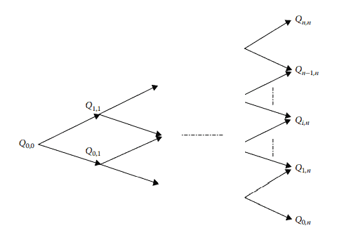
we consider a rather natural binomial tree approximation as illustrated in Figure 5.1, where, without loss of generality, the branching probabilities are uniformly one half.
For notational efficiency, we let
$$
r_{i, n}=r_{0,0}+\Delta t \sum_{k=1}^{n-1} \theta_k+(2 i-n) \sigma \sqrt{\Delta t}, \quad i=0,1, \ldots, n
$$

Then we have a multi-period tree as shown in Figure 5.2.
Before being applied to derivatives pricing, such a tree must first be calibrated to the current term structure of the interest rate. For the Ho-Lee model, we need to determine the drift, $\theta_t$, by reproducing the prices of zero-coupon bonds of all maturities. This task can be efficiently achieved with the help of the so-called Arrow-Debreu prices.

金融代写|利率建模代写Interest Rate Modeling代考|Arrow–Debreu Prices

An Arrow-Debreu (1954) security is a canonical asset that has a cash flow of $\$ 1$ if a particular state (of interest rate) is realized, or nothing otherwise. The pattern of payment is shown in Figure $5.3$, where we let $Q_{i, j}$ denote the price of the security at time 0 that would pay $\$ 1$ at time $j$ if the state $i$ is realized, or nothing if otherwise.

Note that a zero-coupon bond can be regarded as a portfolio of ArrowDebreu securities. By linearity, the price of the zero-coupon bond maturing in time $j$ is equal to
$$
P(0, j)=\sum_{i=0}^j Q_{i, j} .
$$
Given an interest-rate tree as in Figure 5.2, we can construct the ArrowDebreu tree through a forward induction process. We begin with
$$
Q_{0,0}=1 .
$$
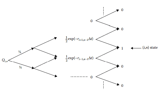
The calculations of $Q_{1,1}$ and $Q_{0,1}$ are done by “expectation pricing” using the trees in Figure $5.4$, where $r_{0,0}$ is the discount rate at node $(0,0)$. Intuitively, the prices of the two Arrow-Debreu securities are given by
$$
Q_{1,1}=Q_{0,1}=\frac{1}{2} \mathrm{e}^{-r_{0,0} \Delta t}
$$

金融代写|利率建模代写Interest Rate Modeling代考|MATH5985

利率建模代考

金融代写|利率建模代写利率建模代考| Ho-Lee模型的二叉树


IIo-Lee模型首先用二叉树表示。对于均值和方差大于$(t, t+\Delta t)$的高斯短期速率模型(
$$
\begin{aligned}
E^{\mathbb{Q}}\left[\Delta r_t\right] &=\theta_t \Delta t \
\operatorname{VaR}\left(\Delta r_t\right) &=\sigma^2 \Delta t
\end{aligned}
$$
),我们考虑一种相当自然的二叉树近似,如图5.1所示,在不丧失一般性的情况下,分支概率一致为1 / 2。
为了符号效率,我们让
$$
r_{i, n}=r_{0,0}+\Delta t \sum_{k=1}^{n-1} \theta_k+(2 i-n) \sigma \sqrt{\Delta t}, \quad i=0,1, \ldots, n
$$


然后我们就有了一个如图5.2所示的多周期树。在应用于衍生品定价之前,这种树必须首先根据当前利率的期限结构进行校准。对于Ho-Lee模型,我们需要通过再现所有期限的零息债券的价格来确定漂移$\theta_t$。在所谓的阿罗-德布鲁价格的帮助下,这一任务可以有效地完成

金融代写|利率建模代写Interest Rate Modeling代考| 阿罗-德布鲁·普莱斯


a Arrow-Debreu(1954)证券是一种典型资产,如果实现了特定的(利率)状态,或者其他什么都没有,那么它的现金流为$\$ 1$。支付模式如图$5.3$所示,其中我们让$Q_{i, j}$表示时间0时的证券价格,如果状态$i$实现,则在时间$j$时支付$\$ 1$,否则则不支付


请注意,零息债券可以被视为ArrowDebreu证券的投资组合。通过线性关系,及时$j$到期的零息债券价格等于
$$
P(0, j)=\sum_{i=0}^j Q_{i, j} .
$$
给定如图5.2所示的利率树,我们可以通过正向归纳过程构建ArrowDebreu树。我们从
$$
Q_{0,0}=1 .
$$
开始,$Q_{1,1}$和$Q_{0,1}$的计算通过使用图$5.4$中的树的“期望定价”来完成,其中$r_{0,0}$是节点$(0,0)$上的贴现率。直观地看,这两种Arrow-Debreu证券的价格由
$$
Q_{1,1}=Q_{0,1}=\frac{1}{2} \mathrm{e}^{-r_{0,0} \Delta t}
$$ 给出

金融代写|利率建模代写Interest Rate Modeling代考 请认准statistics-lab™

统计代写请认准statistics-lab™. statistics-lab™为您的留学生涯保驾护航。

金融工程代写

金融工程是使用数学技术来解决金融问题。金融工程使用计算机科学、统计学、经济学和应用数学领域的工具和知识来解决当前的金融问题,以及设计新的和创新的金融产品。

非参数统计代写

非参数统计指的是一种统计方法,其中不假设数据来自于由少数参数决定的规定模型;这种模型的例子包括正态分布模型和线性回归模型。

广义线性模型代考

广义线性模型(GLM)归属统计学领域,是一种应用灵活的线性回归模型。该模型允许因变量的偏差分布有除了正态分布之外的其它分布。

术语 广义线性模型(GLM)通常是指给定连续和/或分类预测因素的连续响应变量的常规线性回归模型。它包括多元线性回归,以及方差分析和方差分析(仅含固定效应)。

有限元方法代写

有限元方法(FEM)是一种流行的方法,用于数值解决工程和数学建模中出现的微分方程。典型的问题领域包括结构分析、传热、流体流动、质量运输和电磁势等传统领域。

有限元是一种通用的数值方法,用于解决两个或三个空间变量的偏微分方程(即一些边界值问题)。为了解决一个问题,有限元将一个大系统细分为更小、更简单的部分,称为有限元。这是通过在空间维度上的特定空间离散化来实现的,它是通过构建对象的网格来实现的:用于求解的数值域,它有有限数量的点。边界值问题的有限元方法表述最终导致一个代数方程组。该方法在域上对未知函数进行逼近。[1] 然后将模拟这些有限元的简单方程组合成一个更大的方程系统,以模拟整个问题。然后,有限元通过变化微积分使相关的误差函数最小化来逼近一个解决方案。

tatistics-lab作为专业的留学生服务机构,多年来已为美国、英国、加拿大、澳洲等留学热门地的学生提供专业的学术服务,包括但不限于Essay代写,Assignment代写,Dissertation代写,Report代写,小组作业代写,Proposal代写,Paper代写,Presentation代写,计算机作业代写,论文修改和润色,网课代做,exam代考等等。写作范围涵盖高中,本科,研究生等海外留学全阶段,辐射金融,经济学,会计学,审计学,管理学等全球99%专业科目。写作团队既有专业英语母语作者,也有海外名校硕博留学生,每位写作老师都拥有过硬的语言能力,专业的学科背景和学术写作经验。我们承诺100%原创,100%专业,100%准时,100%满意。

随机分析代写


随机微积分是数学的一个分支,对随机过程进行操作。它允许为随机过程的积分定义一个关于随机过程的一致的积分理论。这个领域是由日本数学家伊藤清在第二次世界大战期间创建并开始的。

时间序列分析代写

随机过程,是依赖于参数的一组随机变量的全体,参数通常是时间。 随机变量是随机现象的数量表现,其时间序列是一组按照时间发生先后顺序进行排列的数据点序列。通常一组时间序列的时间间隔为一恒定值(如1秒,5分钟,12小时,7天,1年),因此时间序列可以作为离散时间数据进行分析处理。研究时间序列数据的意义在于现实中,往往需要研究某个事物其随时间发展变化的规律。这就需要通过研究该事物过去发展的历史记录,以得到其自身发展的规律。

回归分析代写

多元回归分析渐进(Multiple Regression Analysis Asymptotics)属于计量经济学领域,主要是一种数学上的统计分析方法,可以分析复杂情况下各影响因素的数学关系,在自然科学、社会和经济学等多个领域内应用广泛。

MATLAB代写

MATLAB 是一种用于技术计算的高性能语言。它将计算、可视化和编程集成在一个易于使用的环境中,其中问题和解决方案以熟悉的数学符号表示。典型用途包括:数学和计算算法开发建模、仿真和原型制作数据分析、探索和可视化科学和工程图形应用程序开发,包括图形用户界面构建MATLAB 是一个交互式系统,其基本数据元素是一个不需要维度的数组。这使您可以解决许多技术计算问题,尤其是那些具有矩阵和向量公式的问题,而只需用 C 或 Fortran 等标量非交互式语言编写程序所需的时间的一小部分。MATLAB 名称代表矩阵实验室。MATLAB 最初的编写目的是提供对由 LINPACK 和 EISPACK 项目开发的矩阵软件的轻松访问,这两个项目共同代表了矩阵计算软件的最新技术。MATLAB 经过多年的发展,得到了许多用户的投入。在大学环境中,它是数学、工程和科学入门和高级课程的标准教学工具。在工业领域,MATLAB 是高效研究、开发和分析的首选工具。MATLAB 具有一系列称为工具箱的特定于应用程序的解决方案。对于大多数 MATLAB 用户来说非常重要,工具箱允许您学习应用专业技术。工具箱是 MATLAB 函数(M 文件)的综合集合,可扩展 MATLAB 环境以解决特定类别的问题。可用工具箱的领域包括信号处理、控制系统、神经网络、模糊逻辑、小波、仿真等。

R语言代写问卷设计与分析代写
PYTHON代写回归分析与线性模型代写
MATLAB代写方差分析与试验设计代写
STATA代写机器学习/统计学习代写
SPSS代写计量经济学代写
EVIEWS代写时间序列分析代写
EXCEL代写深度学习代写
SQL代写各种数据建模与可视化代写

金融代写|利率建模代写Interest Rate Modeling代考|ACTL40004

如果你也在 怎样代写利率建模Interest Rate Modeling这个学科遇到相关的难题,请随时右上角联系我们的24/7代写客服。

利率模型是指一种对利率的运动和演变进行建模的数学方法。它是一种基于市场风险的单因素短利率模型。瓦西克利率模型常用于经济学中,以确定利率在未来的移动方向。

statistics-lab™ 为您的留学生涯保驾护航 在代写利率建模Interest Rate Modeling方面已经树立了自己的口碑, 保证靠谱, 高质且原创的统计Statistics代写服务。我们的专家在代写利率建模Interest Rate Modeling代写方面经验极为丰富,各种代写利率建模Interest Rate Modeling相关的作业也就用不着说。

我们提供的利率建模Interest Rate Modeling及其相关学科的代写,服务范围广, 其中包括但不限于:

  • Statistical Inference 统计推断
  • Statistical Computing 统计计算
  • Advanced Probability Theory 高等概率论
  • Advanced Mathematical Statistics 高等数理统计学
  • (Generalized) Linear Models 广义线性模型
  • Statistical Machine Learning 统计机器学习
  • Longitudinal Data Analysis 纵向数据分析
  • Foundations of Data Science 数据科学基础
金融代写|利率建模代写Interest Rate Modeling代考|ACTL40004

金融代写|利率建模代写Interest Rate Modeling代考| GENERAL MARKOVIAN MODELS

Existing short-rate models are Markovian models. A no-arbitrage shortrate model should also be derived from the HJM framework. However, this can be quite difficult. In this section, we address the opposite question: under what kind of forward-rate volatility specifications should the resulting short-rate model be a Markovian random variable? Answering this question will help us to calibrate and implement a short-rate model more efficiently.
According to Equation 4.21, the short rate can be expressed as
$$
r_t=f(t, t)=f(0, t)+\int_0^t\left[-\boldsymbol{\sigma}^{\mathrm{T}}(s, t) \mathbf{\Sigma}(s, t) \mathrm{d} s+\boldsymbol{\sigma}^{\mathrm{T}}(s, t) \mathrm{d} \mathbf{W}_s\right]
$$

where $\mathbf{W}t$ is the $n$-dimensional Brownian motion under the risk-neutral measure, $\sigma(t, T)$ the forward-rate volatility, and $\boldsymbol{\Sigma}(t, T)$ the volatility of the $T$-maturity zero-coupon bond, given by $\boldsymbol{\Sigma}(t, T)=-\int_t^T \boldsymbol{\sigma}(t, u) \mathrm{d} u$. The stochastic differentiation of the short rate is $$ \begin{aligned} \mathrm{d} r_t=& {\left[f_t(0, t)+\int_0^t\left(-\frac{\partial}{\partial t}\left(\boldsymbol{\sigma}^{\mathrm{T}}(s, t) \boldsymbol{\Sigma}(s, t)\right) \mathrm{d} s+\frac{\partial \boldsymbol{\sigma}^{\mathrm{T}}(s, t)}{\partial t} \mathrm{~d} \mathbf{W}_s\right)\right] \mathrm{d} t } \ &+\boldsymbol{\sigma}^{\mathrm{T}}(t, t) \mathrm{d} \mathbf{W}_t \ =& {\left[f_t(t, T)\right]{T=t} \mathrm{~d} t+\boldsymbol{\sigma}^{\mathrm{T}}(t, t) \mathrm{d}t . } \end{aligned} $$ Based on Equation $5.17$ we can make the following judgment: for the shortrate model to be a Markovian process, we need the drift term, $\left[f_t(t, T)\right]{T=t}$, to be a function of a finite set of state variables that are jointly Markovian in their evolution.

To write the short rate as a function of several state variables, we introduce auxiliary functions
$$
b_i(t, T)=\sigma_i(t, T) \int_t^T \sigma_i(t, s) \mathrm{d} s, \quad i=1,2, \ldots, n .
$$

金融代写|利率建模代写Interest Rate Modeling代考|Monte Carlo Simulations for Options Pricing

Owing to the Markovian property of short-rate models, path simulations by Monte Carlo methods can be carried out efficiently, which is important for pricing exotic and path-dependent options. Take the pricing of the option on a zero-coupon for example. The value can be expressed as
$$
V_t=E_t^{\mathbb{Q}}\left[\mathrm{e}^{-\int_t^T r_s \mathrm{~d} s}(P(T, \tau)-K)^{+}\right], \quad t<T<\tau
$$
where $\mathbb{Q}$ stands for the risk-neutral measure, $r_t$ is given by Equation $5.20$, and the bond price is given by Equation 5.39. Both variables are expressed in terms of $\chi_i(t)$ and $\varphi_i(t), i=1, \ldots, n$, which evolve according to Equation 5.23. The corresponding simulation scheme for $\chi_i(t)$ and $\varphi_i(t)$ is
$$
\begin{aligned}
&\varphi_i(t+\Delta t)-\varphi_i(t)+\left(\sigma_i^2(t, t)-2 \kappa_i(t) \varphi_i(t)\right) \Delta t \
&\chi_i(t+\Delta t)=\chi_i(t)+\left(\varphi_i(t)-\kappa_i(t) \chi_i(t)\right) \mathrm{d} t+\sigma_i(t, t) \Delta W_i(t)
\end{aligned}
$$
which is simply the so-called Euler scheme. The bond option is priced by simulating many payoffs before taking an average.
In Inui and Kijima (1998), the following example is considered:
$$
\boldsymbol{\sigma}(t, T)=\left(\begin{array}{c}
c_1 r_t^\alpha \
c_2 r_t^\beta \mathrm{e}^{-\kappa(T-t)}
\end{array}\right)
$$
where $c_i, i=1,2, \alpha, \beta$, and $\kappa$ are non-negative constants. It can be verified that the components of the volatility vector satisfy
$$
\frac{\partial \sigma_1(t, T)}{\partial T}=0, \quad \frac{\partial \sigma_2(t, T)}{\partial T}=-\kappa \sigma_2(t, T) .
$$

金融代写|利率建模代写Interest Rate Modeling代考|ACTL40004

利率建模代考

金融代写|利率建模代写Interest Rate Modeling代考| 一般马尔可夫模型


现有的短期利率模型是马尔可夫模型。还应该从HJM框架推导出无套利的短期模型。然而,这是相当困难的。在本节中,我们将讨论相反的问题:在什么样的远期利率波动率规范下,所得到的短期利率模型应该是一个马尔可夫随机变量?回答这个问题将有助于我们更有效地校准和实施短期利率模型。根据公式4.21,短期汇率可表示为
$$
r_t=f(t, t)=f(0, t)+\int_0^t\left[-\boldsymbol{\sigma}^{\mathrm{T}}(s, t) \mathbf{\Sigma}(s, t) \mathrm{d} s+\boldsymbol{\sigma}^{\mathrm{T}}(s, t) \mathrm{d} \mathbf{W}_s\right]
$$

where $\mathbf{W}t$ 是 $n$风险中性测度下的-维布朗运动, $\sigma(t, T)$ 远期利率波动 $\boldsymbol{\Sigma}(t, T)$ 波动率 $T$到期零息债券,由 $\boldsymbol{\Sigma}(t, T)=-\int_t^T \boldsymbol{\sigma}(t, u) \mathrm{d} u$。短期汇率的随机微分是 $$ \begin{aligned} \mathrm{d} r_t=& {\left[f_t(0, t)+\int_0^t\left(-\frac{\partial}{\partial t}\left(\boldsymbol{\sigma}^{\mathrm{T}}(s, t) \boldsymbol{\Sigma}(s, t)\right) \mathrm{d} s+\frac{\partial \boldsymbol{\sigma}^{\mathrm{T}}(s, t)}{\partial t} \mathrm{~d} \mathbf{W}_s\right)\right] \mathrm{d} t } \ &+\boldsymbol{\sigma}^{\mathrm{T}}(t, t) \mathrm{d} \mathbf{W}_t \ =& {\left[f_t(t, T)\right]{T=t} \mathrm{~d} t+\boldsymbol{\sigma}^{\mathrm{T}}(t, t) \mathrm{d}t . } \end{aligned} $$ 基于方程 $5.17$ 我们可以做出以下判断:要使短期模型为马尔可夫过程,我们需要漂移项, $\left[f_t(t, T)\right]{T=t}$,是一组有限状态变量的函数,这些状态变量在演化过程中共同具有马尔可夫性 为了将短期汇率写成几个状态变量的函数,我们引入了辅助函数
$$
b_i(t, T)=\sigma_i(t, T) \int_t^T \sigma_i(t, s) \mathrm{d} s, \quad i=1,2, \ldots, n .
$$

金融代写|利率建模代写利率建模代考|期权定价的蒙特卡洛模拟


由于短期利率模型的马尔可夫性质,蒙特卡洛方法可以有效地进行路径模拟,这对奇异和路径相关期权的定价是重要的。以零息票的期权定价为例。取值可以表示为
$$
V_t=E_t^{\mathbb{Q}}\left[\mathrm{e}^{-\int_t^T r_s \mathrm{~d} s}(P(T, \tau)-K)^{+}\right], \quad t<T<\tau
$$
,其中$\mathbb{Q}$表示风险中性测度,$r_t$由式$5.20$给出,债券价格由式5.39给出。两个变量都用$\chi_i(t)$和$\varphi_i(t), i=1, \ldots, n$表示,根据公式5.23进行演化。$\chi_i(t)$和$\varphi_i(t)$对应的模拟方案是
$$
\begin{aligned}
&\varphi_i(t+\Delta t)-\varphi_i(t)+\left(\sigma_i^2(t, t)-2 \kappa_i(t) \varphi_i(t)\right) \Delta t \
&\chi_i(t+\Delta t)=\chi_i(t)+\left(\varphi_i(t)-\kappa_i(t) \chi_i(t)\right) \mathrm{d} t+\sigma_i(t, t) \Delta W_i(t)
\end{aligned}
$$
,这就是所谓的欧拉方案。债券期权的定价是通过在取平均值之前模拟许多支付进行的。在Inui和Kijima(1998)中,考虑以下例子:
$$
\boldsymbol{\sigma}(t, T)=\left(\begin{array}{c}
c_1 r_t^\alpha \
c_2 r_t^\beta \mathrm{e}^{-\kappa(T-t)}
\end{array}\right)
$$
其中$c_i, i=1,2, \alpha, \beta$和$\kappa$是非负常数。可以验证,波动率向量的分量满足
$$
\frac{\partial \sigma_1(t, T)}{\partial T}=0, \quad \frac{\partial \sigma_2(t, T)}{\partial T}=-\kappa \sigma_2(t, T) .
$$

金融代写|利率建模代写Interest Rate Modeling代考 请认准statistics-lab™

统计代写请认准statistics-lab™. statistics-lab™为您的留学生涯保驾护航。

金融工程代写

金融工程是使用数学技术来解决金融问题。金融工程使用计算机科学、统计学、经济学和应用数学领域的工具和知识来解决当前的金融问题,以及设计新的和创新的金融产品。

非参数统计代写

非参数统计指的是一种统计方法,其中不假设数据来自于由少数参数决定的规定模型;这种模型的例子包括正态分布模型和线性回归模型。

广义线性模型代考

广义线性模型(GLM)归属统计学领域,是一种应用灵活的线性回归模型。该模型允许因变量的偏差分布有除了正态分布之外的其它分布。

术语 广义线性模型(GLM)通常是指给定连续和/或分类预测因素的连续响应变量的常规线性回归模型。它包括多元线性回归,以及方差分析和方差分析(仅含固定效应)。

有限元方法代写

有限元方法(FEM)是一种流行的方法,用于数值解决工程和数学建模中出现的微分方程。典型的问题领域包括结构分析、传热、流体流动、质量运输和电磁势等传统领域。

有限元是一种通用的数值方法,用于解决两个或三个空间变量的偏微分方程(即一些边界值问题)。为了解决一个问题,有限元将一个大系统细分为更小、更简单的部分,称为有限元。这是通过在空间维度上的特定空间离散化来实现的,它是通过构建对象的网格来实现的:用于求解的数值域,它有有限数量的点。边界值问题的有限元方法表述最终导致一个代数方程组。该方法在域上对未知函数进行逼近。[1] 然后将模拟这些有限元的简单方程组合成一个更大的方程系统,以模拟整个问题。然后,有限元通过变化微积分使相关的误差函数最小化来逼近一个解决方案。

tatistics-lab作为专业的留学生服务机构,多年来已为美国、英国、加拿大、澳洲等留学热门地的学生提供专业的学术服务,包括但不限于Essay代写,Assignment代写,Dissertation代写,Report代写,小组作业代写,Proposal代写,Paper代写,Presentation代写,计算机作业代写,论文修改和润色,网课代做,exam代考等等。写作范围涵盖高中,本科,研究生等海外留学全阶段,辐射金融,经济学,会计学,审计学,管理学等全球99%专业科目。写作团队既有专业英语母语作者,也有海外名校硕博留学生,每位写作老师都拥有过硬的语言能力,专业的学科背景和学术写作经验。我们承诺100%原创,100%专业,100%准时,100%满意。

随机分析代写


随机微积分是数学的一个分支,对随机过程进行操作。它允许为随机过程的积分定义一个关于随机过程的一致的积分理论。这个领域是由日本数学家伊藤清在第二次世界大战期间创建并开始的。

时间序列分析代写

随机过程,是依赖于参数的一组随机变量的全体,参数通常是时间。 随机变量是随机现象的数量表现,其时间序列是一组按照时间发生先后顺序进行排列的数据点序列。通常一组时间序列的时间间隔为一恒定值(如1秒,5分钟,12小时,7天,1年),因此时间序列可以作为离散时间数据进行分析处理。研究时间序列数据的意义在于现实中,往往需要研究某个事物其随时间发展变化的规律。这就需要通过研究该事物过去发展的历史记录,以得到其自身发展的规律。

回归分析代写

多元回归分析渐进(Multiple Regression Analysis Asymptotics)属于计量经济学领域,主要是一种数学上的统计分析方法,可以分析复杂情况下各影响因素的数学关系,在自然科学、社会和经济学等多个领域内应用广泛。

MATLAB代写

MATLAB 是一种用于技术计算的高性能语言。它将计算、可视化和编程集成在一个易于使用的环境中,其中问题和解决方案以熟悉的数学符号表示。典型用途包括:数学和计算算法开发建模、仿真和原型制作数据分析、探索和可视化科学和工程图形应用程序开发,包括图形用户界面构建MATLAB 是一个交互式系统,其基本数据元素是一个不需要维度的数组。这使您可以解决许多技术计算问题,尤其是那些具有矩阵和向量公式的问题,而只需用 C 或 Fortran 等标量非交互式语言编写程序所需的时间的一小部分。MATLAB 名称代表矩阵实验室。MATLAB 最初的编写目的是提供对由 LINPACK 和 EISPACK 项目开发的矩阵软件的轻松访问,这两个项目共同代表了矩阵计算软件的最新技术。MATLAB 经过多年的发展,得到了许多用户的投入。在大学环境中,它是数学、工程和科学入门和高级课程的标准教学工具。在工业领域,MATLAB 是高效研究、开发和分析的首选工具。MATLAB 具有一系列称为工具箱的特定于应用程序的解决方案。对于大多数 MATLAB 用户来说非常重要,工具箱允许您学习应用专业技术。工具箱是 MATLAB 函数(M 文件)的综合集合,可扩展 MATLAB 环境以解决特定类别的问题。可用工具箱的领域包括信号处理、控制系统、神经网络、模糊逻辑、小波、仿真等。

R语言代写问卷设计与分析代写
PYTHON代写回归分析与线性模型代写
MATLAB代写方差分析与试验设计代写
STATA代写机器学习/统计学习代写
SPSS代写计量经济学代写
EVIEWS代写时间序列分析代写
EXCEL代写深度学习代写
SQL代写各种数据建模与可视化代写

金融代写|利率建模代写Interest Rate Modeling代考|ACTL90003

如果你也在 怎样代写利率建模Interest Rate Modeling这个学科遇到相关的难题,请随时右上角联系我们的24/7代写客服。

利率模型是指一种对利率的运动和演变进行建模的数学方法。它是一种基于市场风险的单因素短利率模型。瓦西克利率模型常用于经济学中,以确定利率在未来的移动方向。

statistics-lab™ 为您的留学生涯保驾护航 在代写利率建模Interest Rate Modeling方面已经树立了自己的口碑, 保证靠谱, 高质且原创的统计Statistics代写服务。我们的专家在代写利率建模Interest Rate Modeling代写方面经验极为丰富,各种代写利率建模Interest Rate Modeling相关的作业也就用不着说。

我们提供的利率建模Interest Rate Modeling及其相关学科的代写,服务范围广, 其中包括但不限于:

  • Statistical Inference 统计推断
  • Statistical Computing 统计计算
  • Advanced Probability Theory 高等概率论
  • Advanced Mathematical Statistics 高等数理统计学
  • (Generalized) Linear Models 广义线性模型
  • Statistical Machine Learning 统计机器学习
  • Longitudinal Data Analysis 纵向数据分析
  • Foundations of Data Science 数据科学基础
金融代写|利率建模代写Interest Rate Modeling代考|ACTL90003

金融代写|利率建模代写Interest Rate Modeling代考| ON THE LOGNORMAL SPECIFICATION OF FORWARD RATES

We now explore the possibility of using the state-dependent volatility function in the HJM model. Without loss of generality, we consider the forward-rate volatility function of the form
$$
\sigma(t, T)=\sigma_0(t, T) f^\alpha(t, T),
$$

where $\sigma_0(t, T)$ is a deterministic function and $\alpha$ a positive exponent. In the special case, $\alpha=0$, we obtain a Gaussian model.

Similar to Avellaneda and Laurence (1999), we show that the “lognormal” model, corresponding to $\alpha=1$, blows up in finite time in the sense that a forward rate reaches infinity. This result was first obtained by Morton (1988). One can imagine that similar results may apply to the case of $\alpha>0$. Hence, volatility specification in the form of Equation $4.136$ is denied.

It suffices to show the result with a one-factor model. The no-arbitrage condition dictates that the drift must be
$$
\mu(t, T)=f(t, T) \sigma_0(t, T) \int_t^T f(t, s) \sigma_0(t, s) \mathrm{d} s,
$$
which depends on the entire curve of $f(t, s), t \leq s \leq T$. Consider the simplest specification of $\sigma_0(t, T)$ : $\sigma_0(t, T)=\sigma_0=$ constant. The HJM equation then becomes
$$
\frac{\mathrm{d} f(t, T)}{f(t, T)}=\sigma_0 \mathrm{~d} \tilde{W}_t+\left(\sigma_0^2 \int_t^T f(t, s) \mathrm{d} s\right) \mathrm{d} t .
$$
The formal solution to the above equation is
$$
\begin{aligned}
f(t, T) &=f(0, T) \exp \left(\sigma_0 \tilde{W}_t-\frac{\sigma_0^2}{2} t+\sigma_0^2 \int_0^t\left(\int_s^T f(s, u) \mathrm{d} u\right) \mathrm{d} s\right) \
&=f(0, T) M(t) \exp \left(\sigma_0^2 \int_0^t\left(\int_s^T f(s, u) \mathrm{d} u\right) \mathrm{d} s\right)
\end{aligned}
$$ where $M(t)=\exp \left(\sigma_0 \tilde{W}_t-\left(\sigma_0^2 / 2\right) t\right)$. Assume for simplicity that the initial term structure is flat, that is, $f(0, T)=f_0=$ constant.

金融代写|利率建模代写Interest Rate Modeling代考|FROM SHORT-RATE MODELS TO FORWARD-RATE MODELS

Short-rate models dominated fixed-income modeling before the emergence of the no-arbitrage framework of Heath, Jarrow, and Morton (1992), which is based on forward rates. Short-rate models can be made arbitrage free by taking appropriate drift terms, such as the Ho-Lee model and the I Iull-White model. But this is not always easy. One way to derive the correct drift term is to identify the corresponding forward-rate volatility and then to solve for the expression of the forward rates, which include the short rate as an extreme case, from the HJM equation. The focus in this section is on how to derive the corresponding forward-rate volatility in order to identify the model as a special case of the HJM framework.

Consider in general an Ito’s process for the short rate under the riskneutral measure, $\mathbb{Q}$,
$$
\mathrm{d} r_t=v\left(r_t, t\right) \mathrm{d} t+\rho\left(r_t, t\right) \mathrm{d} W_t,
$$ where the drift, $v\left(r_t, t\right)$, and volatility, $\rho\left(r_t, t\right)$, are deterministic functions of their arguments. Note that, for notational simplicity, we hereafter drop ” $\sim$ ” over the $\mathbb{Q}$-Brownian motion, $W_t$. Define an auxiliary function
$$
g(x, t, T)=-\ln E^{\mathbb{Q}}\left[\exp \left(-\int_t^T r_s \mathrm{~d} s\right) \mid r_t=x\right]
$$
We have the following result (Baxter and Rennie, 1996).

金融代写|利率建模代写Interest Rate Modeling代考|ACTL90003

利率建模代考

金融代写|利率建模代写Interest Rate Modeling代考| 关于远期汇率的对数正规规范


我们现在探讨在HJM模型中使用状态相关波动函数的可能性。在不失一般性的前提下,我们考虑远期汇率波动函数的形式为
$$
\sigma(t, T)=\sigma_0(t, T) f^\alpha(t, T),
$$

其中$\sigma_0(t, T)$是一个确定性函数,$\alpha$是一个正指数。在特殊情况下,$\alpha=0$,我们得到一个高斯模型 与Avellaneda和Laurence(1999)类似,我们证明了对应于$\alpha=1$的“对数正态”模型,在正向速率达到无穷大的意义上,会在有限时间内崩溃。这个结果是由Morton(1988)首先得到的。可以想象,类似的结果可能适用于$\alpha>0$的情况。因此,公式$4.136$形式的波动率说明被否定。


用单因素模型显示结果就足够了。无套利条件规定漂移必须
$$
\mu(t, T)=f(t, T) \sigma_0(t, T) \int_t^T f(t, s) \sigma_0(t, s) \mathrm{d} s,
$$
,这取决于$f(t, s), t \leq s \leq T$的整条曲线。考虑$\sigma_0(t, T)$: $\sigma_0(t, T)=\sigma_0=$常量的最简单规范。HJM方程于是变成
$$
\frac{\mathrm{d} f(t, T)}{f(t, T)}=\sigma_0 \mathrm{~d} \tilde{W}_t+\left(\sigma_0^2 \int_t^T f(t, s) \mathrm{d} s\right) \mathrm{d} t .
$$
上面方程的形式解是
$$
\begin{aligned}
f(t, T) &=f(0, T) \exp \left(\sigma_0 \tilde{W}_t-\frac{\sigma_0^2}{2} t+\sigma_0^2 \int_0^t\left(\int_s^T f(s, u) \mathrm{d} u\right) \mathrm{d} s\right) \
&=f(0, T) M(t) \exp \left(\sigma_0^2 \int_0^t\left(\int_s^T f(s, u) \mathrm{d} u\right) \mathrm{d} s\right)
\end{aligned}
$$,其中$M(t)=\exp \left(\sigma_0 \tilde{W}_t-\left(\sigma_0^2 / 2\right) t\right)$。为简单起见,假设初始期限结构是平坦的,即$f(0, T)=f_0=$常数。

金融代写|利率建模代写Interest Rate Modeling代考|从短期利率模型到远期利率模型


在Heath、Jarrow和Morton(1992)提出基于远期利率的无套利框架之前,短期利率模型在固定收益模型中占主导地位。采用适当的漂移项可以使短期利率模型无套利,如Ho-Lee模型和I Iull-White模型。但这并不总是容易的。推导正确漂移项的一种方法是确定相应的远期汇率波动率,然后从HJM方程求解远期汇率的表达式,其中包括短期汇率作为一个极端情况。本节的重点是如何推导出相应的远期汇率波动率,以便将模型识别为HJM框架的特例

一般地考虑在风险中性度量下的短期汇率的伊藤过程$\mathbb{Q}$,
$$
\mathrm{d} r_t=v\left(r_t, t\right) \mathrm{d} t+\rho\left(r_t, t\right) \mathrm{d} W_t,
$$,其中漂移,$v\left(r_t, t\right)$和波动率,$\rho\left(r_t, t\right)$是其参数的确定性函数。注意,为了表示法的简单性,我们以后在$\mathbb{Q}$ -布朗运动$W_t$上省略“$\sim$”。定义一个辅助函数
$$
g(x, t, T)=-\ln E^{\mathbb{Q}}\left[\exp \left(-\int_t^T r_s \mathrm{~d} s\right) \mid r_t=x\right]
$$
我们得到以下结果(Baxter和Rennie, 1996)

金融代写|利率建模代写Interest Rate Modeling代考 请认准statistics-lab™

统计代写请认准statistics-lab™. statistics-lab™为您的留学生涯保驾护航。

金融工程代写

金融工程是使用数学技术来解决金融问题。金融工程使用计算机科学、统计学、经济学和应用数学领域的工具和知识来解决当前的金融问题,以及设计新的和创新的金融产品。

非参数统计代写

非参数统计指的是一种统计方法,其中不假设数据来自于由少数参数决定的规定模型;这种模型的例子包括正态分布模型和线性回归模型。

广义线性模型代考

广义线性模型(GLM)归属统计学领域,是一种应用灵活的线性回归模型。该模型允许因变量的偏差分布有除了正态分布之外的其它分布。

术语 广义线性模型(GLM)通常是指给定连续和/或分类预测因素的连续响应变量的常规线性回归模型。它包括多元线性回归,以及方差分析和方差分析(仅含固定效应)。

有限元方法代写

有限元方法(FEM)是一种流行的方法,用于数值解决工程和数学建模中出现的微分方程。典型的问题领域包括结构分析、传热、流体流动、质量运输和电磁势等传统领域。

有限元是一种通用的数值方法,用于解决两个或三个空间变量的偏微分方程(即一些边界值问题)。为了解决一个问题,有限元将一个大系统细分为更小、更简单的部分,称为有限元。这是通过在空间维度上的特定空间离散化来实现的,它是通过构建对象的网格来实现的:用于求解的数值域,它有有限数量的点。边界值问题的有限元方法表述最终导致一个代数方程组。该方法在域上对未知函数进行逼近。[1] 然后将模拟这些有限元的简单方程组合成一个更大的方程系统,以模拟整个问题。然后,有限元通过变化微积分使相关的误差函数最小化来逼近一个解决方案。

tatistics-lab作为专业的留学生服务机构,多年来已为美国、英国、加拿大、澳洲等留学热门地的学生提供专业的学术服务,包括但不限于Essay代写,Assignment代写,Dissertation代写,Report代写,小组作业代写,Proposal代写,Paper代写,Presentation代写,计算机作业代写,论文修改和润色,网课代做,exam代考等等。写作范围涵盖高中,本科,研究生等海外留学全阶段,辐射金融,经济学,会计学,审计学,管理学等全球99%专业科目。写作团队既有专业英语母语作者,也有海外名校硕博留学生,每位写作老师都拥有过硬的语言能力,专业的学科背景和学术写作经验。我们承诺100%原创,100%专业,100%准时,100%满意。

随机分析代写


随机微积分是数学的一个分支,对随机过程进行操作。它允许为随机过程的积分定义一个关于随机过程的一致的积分理论。这个领域是由日本数学家伊藤清在第二次世界大战期间创建并开始的。

时间序列分析代写

随机过程,是依赖于参数的一组随机变量的全体,参数通常是时间。 随机变量是随机现象的数量表现,其时间序列是一组按照时间发生先后顺序进行排列的数据点序列。通常一组时间序列的时间间隔为一恒定值(如1秒,5分钟,12小时,7天,1年),因此时间序列可以作为离散时间数据进行分析处理。研究时间序列数据的意义在于现实中,往往需要研究某个事物其随时间发展变化的规律。这就需要通过研究该事物过去发展的历史记录,以得到其自身发展的规律。

回归分析代写

多元回归分析渐进(Multiple Regression Analysis Asymptotics)属于计量经济学领域,主要是一种数学上的统计分析方法,可以分析复杂情况下各影响因素的数学关系,在自然科学、社会和经济学等多个领域内应用广泛。

MATLAB代写

MATLAB 是一种用于技术计算的高性能语言。它将计算、可视化和编程集成在一个易于使用的环境中,其中问题和解决方案以熟悉的数学符号表示。典型用途包括:数学和计算算法开发建模、仿真和原型制作数据分析、探索和可视化科学和工程图形应用程序开发,包括图形用户界面构建MATLAB 是一个交互式系统,其基本数据元素是一个不需要维度的数组。这使您可以解决许多技术计算问题,尤其是那些具有矩阵和向量公式的问题,而只需用 C 或 Fortran 等标量非交互式语言编写程序所需的时间的一小部分。MATLAB 名称代表矩阵实验室。MATLAB 最初的编写目的是提供对由 LINPACK 和 EISPACK 项目开发的矩阵软件的轻松访问,这两个项目共同代表了矩阵计算软件的最新技术。MATLAB 经过多年的发展,得到了许多用户的投入。在大学环境中,它是数学、工程和科学入门和高级课程的标准教学工具。在工业领域,MATLAB 是高效研究、开发和分析的首选工具。MATLAB 具有一系列称为工具箱的特定于应用程序的解决方案。对于大多数 MATLAB 用户来说非常重要,工具箱允许您学习应用专业技术。工具箱是 MATLAB 函数(M 文件)的综合集合,可扩展 MATLAB 环境以解决特定类别的问题。可用工具箱的领域包括信号处理、控制系统、神经网络、模糊逻辑、小波、仿真等。

R语言代写问卷设计与分析代写
PYTHON代写回归分析与线性模型代写
MATLAB代写方差分析与试验设计代写
STATA代写机器学习/统计学习代写
SPSS代写计量经济学代写
EVIEWS代写时间序列分析代写
EXCEL代写深度学习代写
SQL代写各种数据建模与可视化代写

金融代写|金融数学代写Financial Mathematics代考|MATH3090

如果你也在 怎样代写金融数学Financial Mathematics这个学科遇到相关的难题,请随时右上角联系我们的24/7代写客服。

金融数学是将数学方法应用于金融问题。(有时使用的同等名称是定量金融、金融工程、数学金融和计算金融)。它借鉴了概率、统计、随机过程和经济理论的工具。传统上,投资银行、商业银行、对冲基金、保险公司、公司财务部和监管机构将金融数学的方法应用于诸如衍生证券估值、投资组合结构、风险管理和情景模拟等问题。依赖商品的行业(如能源、制造业)也使用金融数学。 定量分析为金融市场和投资过程带来了效率和严谨性,在监管方面也变得越来越重要。

statistics-lab™ 为您的留学生涯保驾护航 在代写金融数学Financial Mathematics方面已经树立了自己的口碑, 保证靠谱, 高质且原创的统计Statistics代写服务。我们的专家在代写金融数学Financial Mathematics代写方面经验极为丰富,各种代写金融数学Financial Mathematics相关的作业也就用不着说。

我们提供的金融数学Financial Mathematics及其相关学科的代写,服务范围广, 其中包括但不限于:

  • Statistical Inference 统计推断
  • Statistical Computing 统计计算
  • Advanced Probability Theory 高等概率论
  • Advanced Mathematical Statistics 高等数理统计学
  • (Generalized) Linear Models 广义线性模型
  • Statistical Machine Learning 统计机器学习
  • Longitudinal Data Analysis 纵向数据分析
  • Foundations of Data Science 数据科学基础
金融代写|金融数学代写Financial Mathematics代考|MATH3090

金融代写|金融数学代写Financial Mathematics代考|The Limits to Arbitrage and Complete Markets

The models and intuition of earlier sections often relied on or described prices in frictionless markets wherein numerous investors such as speculators and arbitragers compete to earn higher returns. Financial economists often describe this condition of informational market efficiency as being when all available information becomes reflected in market prices such that it is not possible to utilize that information to consistently earn a riskadjusted abnormal profit (i.e., market participants cannot consistently identify mispriced securities).
A well-recognized problem with the theory of informationally efficient markets is that if available information is instantaneously incorporated into market prices then there will be no incentive for market participants to gather information and integrate that information into their investment decisions. If no one searches for mispriced securities then prices will not be efficient. In a perfectly efficient market everyone would adopt passive investment strategies which are buy-and-hold strategies with no attempt to trade in an effort to gain from mispriced securities.
Clearly no market can be perfectly efficient. The only meaningful issue is the extent to which markets approach informational efficiency.

The concept of inefficiently efficient markets is that securities are mispriced just enough and just often enough to attract a moderate number of active investment managers (managers that execute trades for the purpose of trying to improve risk-adjusted return) and active individual investors. The benefits and costs of active investing reach an equilibrium that results in a level of market inefficiency that sustains this equilibrium level of information analysis.

The primary purpose of derivatives is to facilitate risk management. Financial derivatives help to complete a market. Perfect completion of a market means that there are enough distinct investment opportunities available that investors can establish long and short positions in existing securities in a way that allows them to position their portfolio exactly as they desire. As an example, if a grocery store mixes apples, bananas, and cherries into three different types of fruit baskets, a customer may be inconvenienced by being unable to purchase one basket with exactly the amount of each type of fruit that she desires unless by chance one of the baskets exactly meets her preferences. However, if a customer is allowed to trade with the store and can buy and sell the different types of fruit baskets without trading costs, she will be able to obtain exactly the numbers of each type of fruit that she desires so long as the number of distinct fruit baskets being traded equals the number of different types of fruit (i.e., the market is complete). In a similar way, derivatives are created to move the market closer to completion so that market participants are better able to establish positions that move the participants closer to their desired risk exposures.
Financial derivatives can also be used to provide arbitragers, speculators, and investors with powerful tools with which to attempt to enhance their risk-adjusted returns through superior processing of available information. When those market participants with the greatest abilities to identify mispriced securities are enabled with superior tools such as derivatives to best utilize their abilities to buy underpriced assets and sell overpriced assets, the market prices of assets will tend to be better driven toward their intrinsic values. Because market prices provide the signals that guide production and consumption decisions throughout an economy, these arbitragers, speculators, and investors are unwittingly driving the decision making throughout the entire economy into being more and more efficient. Therefore, derivatives can play a role in increasing the efficiency in production and consumption decisions which in turn means improved economic growth and economic utility.

金融代写|金融数学代写Financial Mathematics代考|Chapter Demonstrating Exercises

A U.S.-based export firm will receive 10 million British pounds in three months. The firm can tolerate an exchange rate between $\$ 1.25$ to $\$ 1.34$ U.S. dollars per pound to convert the pounds to its domestic currency (U.S. dollars), but is unwilling to bear the risk of converting the foreign exchange to U.S. dollars at an exchange rate of $\$ 1.25$ or lower. On the other hand, the firm will be very content with an exchange rate of $\$ 1.34$ per British pound. How can a financial derivative strategy be designed to meet the needs of this U.S. export firm?
To hedge the downside risk, the firm can enter an option contract to exchange the 10 million British pounds for U.S. dollars at $\$ 1.25$ per pound. The company can raise some or all of the money to finance this option purchase by writing a call option allowing the option buyer to convert 10 million British pounds to U.S. dollars at a rate of $\$ 1.34$. From the perspective of U.S. dollars the option with a strike rate of $\$ 1.25 \mathrm{might}$ be more clearly viewed as a long put (allowing the U.S. company to put foreign exchange for U.S. dollars) and the option with a strike price of $\$ 1.34$ is short a call (allowing the counterparty to buy the British pounds from the U.S. company for $\$ 1.34$ per pound). But in practice the conventions for designating FX options as calls or puts vary and are driven by local conventions.
Strategy: Long a 1.25\$/pound put, short a $1.34 \$$ /pound call
Table $1.4$ illustrates financial outcomes over the range of possible exchange rates.

金融代写|金融数学代写Financial Mathematics代考|MATH3090

金融数学代考

金融代写|金融数学代写金融数学代考|套利和完全市场的极限


前面几节的模型和直觉通常依赖或描述无摩擦市场中的价格,在这个市场中,大量的投资者,如投机者和套利者,竞相获得更高的回报。金融经济学家通常将这种信息市场效率的条件描述为:当所有可用的信息都反映在市场价格中,这样就不可能利用这些信息持续获得风险调整后的异常利润(即,市场参与者无法持续识别定价错误的证券)。信息有效市场理论的一个众所周知的问题是,如果可获得的信息立即被纳入市场价格,那么市场参与者就没有动力去收集信息并将这些信息整合到他们的投资决策中。如果没有人去寻找定价错误的证券,那么价格就不会有效。在一个完全有效的市场中,每个人都会采用被动投资策略,即买入并持有策略,不试图从定价错误的证券中获利。显然,没有一个市场是完全有效的。唯一有意义的问题是市场在多大程度上接近信息效率


低效率高效市场的概念是,证券的错误定价刚好足够,而且经常刚好足够吸引适量的积极投资经理(执行交易的经理,目的是试图提高风险调整后的回报)和积极的个人投资者。积极投资的收益和成本达到一种均衡,导致一定程度的市场效率低下,从而维持这种均衡水平的信息分析


衍生品的主要目的是促进风险管理。金融衍生品有助于完善市场。市场的完美完成意味着有足够多的明显的投资机会,投资者可以在现有证券中建立多头和空头头寸,从而使他们能够完全按照自己的意愿配置投资组合。例如,如果一家杂货店将苹果、香蕉和樱桃混合到三个不同类型的果篮中,顾客可能会因为无法购买一篮子她想要的每种类型水果的数量而感到不便,除非恰巧其中一个篮子正好满足她的偏好。然而,如果一个顾客被允许与商店进行交易,并且可以在没有交易成本的情况下买卖不同类型的果篮,那么只要被交易的不同果篮的数量等于不同类型的水果的数量(即,市场是完整的),她就能够确切地获得她想要的每种类型的水果的数量。以类似的方式,衍生品的创造是为了使市场更接近完成,从而使市场参与者能够更好地建立头寸,使参与者更接近他们期望的风险敞口。金融衍生品也可以被用来为套利者、投机者和投资者提供强大的工具,试图通过对现有信息的卓越处理来提高其经风险调整后的收益。当那些最有能力识别错误定价证券的市场参与者能够使用高级工具(如衍生品)来最好地利用他们的能力购买定价过低的资产和出售定价过高的资产时,资产的市场价格将倾向于更好地推动其内在价值。由于市场价格提供了指导整个经济的生产和消费决策的信号,这些套利者、投机者和投资者正在不知不觉中推动整个经济的决策变得越来越高效。因此,衍生品可以在提高生产和消费决策的效率方面发挥作用,这反过来意味着改善经济增长和经济效用

金融代写|金融数学代写Financial Mathematics代考|示范练习


一家美国出口公司将在三个月内收到1000万英镑。该公司可以容忍每磅汇率在$\$ 1.25$到$\$ 1.34$美元之间,将英镑转换为本国货币(美元),但不愿意承担以$\$ 1.25$或更低的汇率将外汇转换为美元的风险。另一方面,公司对每英镑$\$ 1.34$的汇率也很满意。如何设计金融衍生品策略来满足美国出口公司的需求?为了对冲下行风险,该公司可以签订一份期权合同,以每磅$\$ 1.25$的价格将1000万英镑兑换成美元。该公司可以通过编写看涨期权来筹集部分或全部资金,允许期权买家将1000万英镑以$\$ 1.34$的汇率兑换成美元。从美元的角度来看,执行率为$\$ 1.25 \mathrm{might}$的期权可以更清楚地看作是一个看跌期权(允许美国公司将外汇兑换成美元),执行价为$\$ 1.34$的期权则是一个看涨期权(允许交易对手以每磅$\$ 1.34$的价格从美国公司购买英镑)。但在实践中,将外汇期权指定为看涨期权或看跌期权的惯例各不相同,并受当地惯例的影响。策略:做多1.25美元/磅看跌期权,做空$1.34 \$$ /磅看涨期权
表$1.4$说明了在可能的汇率范围内的财务结果

金融代写|金融数学代写Financial Mathematics代考 请认准statistics-lab™

统计代写请认准statistics-lab™. statistics-lab™为您的留学生涯保驾护航。

金融工程代写

金融工程是使用数学技术来解决金融问题。金融工程使用计算机科学、统计学、经济学和应用数学领域的工具和知识来解决当前的金融问题,以及设计新的和创新的金融产品。

非参数统计代写

非参数统计指的是一种统计方法,其中不假设数据来自于由少数参数决定的规定模型;这种模型的例子包括正态分布模型和线性回归模型。

广义线性模型代考

广义线性模型(GLM)归属统计学领域,是一种应用灵活的线性回归模型。该模型允许因变量的偏差分布有除了正态分布之外的其它分布。

术语 广义线性模型(GLM)通常是指给定连续和/或分类预测因素的连续响应变量的常规线性回归模型。它包括多元线性回归,以及方差分析和方差分析(仅含固定效应)。

有限元方法代写

有限元方法(FEM)是一种流行的方法,用于数值解决工程和数学建模中出现的微分方程。典型的问题领域包括结构分析、传热、流体流动、质量运输和电磁势等传统领域。

有限元是一种通用的数值方法,用于解决两个或三个空间变量的偏微分方程(即一些边界值问题)。为了解决一个问题,有限元将一个大系统细分为更小、更简单的部分,称为有限元。这是通过在空间维度上的特定空间离散化来实现的,它是通过构建对象的网格来实现的:用于求解的数值域,它有有限数量的点。边界值问题的有限元方法表述最终导致一个代数方程组。该方法在域上对未知函数进行逼近。[1] 然后将模拟这些有限元的简单方程组合成一个更大的方程系统,以模拟整个问题。然后,有限元通过变化微积分使相关的误差函数最小化来逼近一个解决方案。

tatistics-lab作为专业的留学生服务机构,多年来已为美国、英国、加拿大、澳洲等留学热门地的学生提供专业的学术服务,包括但不限于Essay代写,Assignment代写,Dissertation代写,Report代写,小组作业代写,Proposal代写,Paper代写,Presentation代写,计算机作业代写,论文修改和润色,网课代做,exam代考等等。写作范围涵盖高中,本科,研究生等海外留学全阶段,辐射金融,经济学,会计学,审计学,管理学等全球99%专业科目。写作团队既有专业英语母语作者,也有海外名校硕博留学生,每位写作老师都拥有过硬的语言能力,专业的学科背景和学术写作经验。我们承诺100%原创,100%专业,100%准时,100%满意。

随机分析代写


随机微积分是数学的一个分支,对随机过程进行操作。它允许为随机过程的积分定义一个关于随机过程的一致的积分理论。这个领域是由日本数学家伊藤清在第二次世界大战期间创建并开始的。

时间序列分析代写

随机过程,是依赖于参数的一组随机变量的全体,参数通常是时间。 随机变量是随机现象的数量表现,其时间序列是一组按照时间发生先后顺序进行排列的数据点序列。通常一组时间序列的时间间隔为一恒定值(如1秒,5分钟,12小时,7天,1年),因此时间序列可以作为离散时间数据进行分析处理。研究时间序列数据的意义在于现实中,往往需要研究某个事物其随时间发展变化的规律。这就需要通过研究该事物过去发展的历史记录,以得到其自身发展的规律。

回归分析代写

多元回归分析渐进(Multiple Regression Analysis Asymptotics)属于计量经济学领域,主要是一种数学上的统计分析方法,可以分析复杂情况下各影响因素的数学关系,在自然科学、社会和经济学等多个领域内应用广泛。

MATLAB代写

MATLAB 是一种用于技术计算的高性能语言。它将计算、可视化和编程集成在一个易于使用的环境中,其中问题和解决方案以熟悉的数学符号表示。典型用途包括:数学和计算算法开发建模、仿真和原型制作数据分析、探索和可视化科学和工程图形应用程序开发,包括图形用户界面构建MATLAB 是一个交互式系统,其基本数据元素是一个不需要维度的数组。这使您可以解决许多技术计算问题,尤其是那些具有矩阵和向量公式的问题,而只需用 C 或 Fortran 等标量非交互式语言编写程序所需的时间的一小部分。MATLAB 名称代表矩阵实验室。MATLAB 最初的编写目的是提供对由 LINPACK 和 EISPACK 项目开发的矩阵软件的轻松访问,这两个项目共同代表了矩阵计算软件的最新技术。MATLAB 经过多年的发展,得到了许多用户的投入。在大学环境中,它是数学、工程和科学入门和高级课程的标准教学工具。在工业领域,MATLAB 是高效研究、开发和分析的首选工具。MATLAB 具有一系列称为工具箱的特定于应用程序的解决方案。对于大多数 MATLAB 用户来说非常重要,工具箱允许您学习应用专业技术。工具箱是 MATLAB 函数(M 文件)的综合集合,可扩展 MATLAB 环境以解决特定类别的问题。可用工具箱的领域包括信号处理、控制系统、神经网络、模糊逻辑、小波、仿真等。

R语言代写问卷设计与分析代写
PYTHON代写回归分析与线性模型代写
MATLAB代写方差分析与试验设计代写
STATA代写机器学习/统计学习代写
SPSS代写计量经济学代写
EVIEWS代写时间序列分析代写
EXCEL代写深度学习代写
SQL代写各种数据建模与可视化代写

金融代写|金融数学代写Financial Mathematics代考|ACTL20001

如果你也在 怎样代写金融数学Financial Mathematics这个学科遇到相关的难题,请随时右上角联系我们的24/7代写客服。

金融数学是将数学方法应用于金融问题。(有时使用的同等名称是定量金融、金融工程、数学金融和计算金融)。它借鉴了概率、统计、随机过程和经济理论的工具。传统上,投资银行、商业银行、对冲基金、保险公司、公司财务部和监管机构将金融数学的方法应用于诸如衍生证券估值、投资组合结构、风险管理和情景模拟等问题。依赖商品的行业(如能源、制造业)也使用金融数学。 定量分析为金融市场和投资过程带来了效率和严谨性,在监管方面也变得越来越重要。

statistics-lab™ 为您的留学生涯保驾护航 在代写金融数学Financial Mathematics方面已经树立了自己的口碑, 保证靠谱, 高质且原创的统计Statistics代写服务。我们的专家在代写金融数学Financial Mathematics代写方面经验极为丰富,各种代写金融数学Financial Mathematics相关的作业也就用不着说。

我们提供的金融数学Financial Mathematics及其相关学科的代写,服务范围广, 其中包括但不限于:

  • Statistical Inference 统计推断
  • Statistical Computing 统计计算
  • Advanced Probability Theory 高等概率论
  • Advanced Mathematical Statistics 高等数理统计学
  • (Generalized) Linear Models 广义线性模型
  • Statistical Machine Learning 统计机器学习
  • Longitudinal Data Analysis 纵向数据分析
  • Foundations of Data Science 数据科学基础
金融代写|金融数学代写Financial Mathematics代考|ACTL20001

金融代写|金融数学代写Financial Mathematics代考|Option Combination Strategies

Option combinations involve simultaneous positions in at least one call option and at least one put option. This section focuses on combinations of calls and puts with the same expiration date and underlying asset. The synthetic long positions in the underlying asset using options (long a call and short a put) and short positions (long a put and short a call) discussed in Section $1.8 .1$ are option combinations. This section discusses others.

Option straddles have equally sized simultaneous long positions or simultaneous short positions in call and put options with the same strike price (and same expiration date). Figure $1.12$ illustrates the profitability of a long straddle at expiration with a solid line and shows the underlying components of long a call and long a put with dashed lines. The value of a long straddle is positively exposed to the volatility of the underlying asset. A short straddle is the mirror image (i.e., the maximum profit is above $K$ with losses on the far right and left).

Option strangles are similar to option straddles, except the call and put options have different strike prices. Figure $1.13$ illustrates a long strangle. Other options strategies can involve option portfolios such as ratio spreads with more calls than puts or vice versa such that the payoffs differ in different directions.

金融代写|金融数学代写Financial Mathematics代考|Other Options

There are many types of stand-alone options on financial assets that differ from simple calls and puts. Some options allow exercise at several specific points in time (a Bermuda option), some are based on functions of prices such as averages or extremes (e.g., Asian options have payoffs based on averaged prices of the underlying asset). Some options cease to exist if the underlying asset reaches a particular level or become exercisable if the underlying asset reaches a particular level such as barrier options.
Financial markets and economic activity in general are full of options. There are options on real assets such as options to: buy land, rent space, return products, extend warrantees, take early retirement, terminate contracts, and on and on.

There are non-traded financial options such as options to pre-pay mortgages and other loans, options to break some bank certificates of deposits (i.e., receive early termination), options to rollover some bank deposits, options to cash out insurance policies, options to increase insurance coverage, and so forth.

The common stock of a leveraged corporation can be viewed as a call option on the corporation’s stock. There are even options on options known as compound options.
Two things to keep in mind are this: (1) there are countless implicit and explicit options in a modern economy because those options serve important purposes of allowing participants to manage and control their risk exposures and (2) the astounding variety and complexity of these important contracts creates demand for people with mathematical modeling skills, especially those who can create innovations or at least understand and model the innovations. This book touches on the most common options in existence today. No one can yet imagine the options that will emerge in the future to meet the changing needs of our rapidly changing world.

金融代写|金融数学代写Financial Mathematics代考|ACTL20001

金融数学代考

金融代写|金融数学代写金融数学代考|选项组合策略

. .


期权组合包括至少一个看涨期权和至少一个看跌期权的同时头寸。本节重点介绍具有相同到期日和标的资产的看涨期权和看跌期权的组合。使用期权在标的资产中合成的多头头寸(做多看涨期权和做空看跌期权)和做空头寸(做多看跌期权和做空看涨期权)在$1.8 .1$节中讨论的是期权组合。


期权跨空具有相同执行价格(和相同到期日)的看涨期权和看跌期权的同时多头头寸或同时空头头寸。图$1.12$用实线说明了到期时多头跨空期权的盈利能力,用虚线显示了多头看涨期权和多头看跌期权的基本组成部分。多头多头的价值受到标的资产波动的正面影响。空头跨空是镜像(即最大利润在$K$以上,亏损在最右和最左)


除了看涨期权和看跌期权的执行价格不同之外,期权绞杀期权与期权跨空期权类似。图$1.13$说明了一个长时间的扼杀。其他期权策略可以包括期权组合,如看涨期权多于看跌期权,反之亦然,从而使不同方向的收益不同

金融代写|金融数学代写金融数学代考|其他选项

.


金融资产的独立期权有许多类型,不同于简单的看涨期权和看跌期权。有些期权允许在几个特定的时间点执行(百慕大期权),有些则基于价格的函数,如平均值或极值(例如,亚洲期权的支付基于标的资产的平均价格)。如果标的资产达到特定水平,则有些期权将不复存在;如果标的资产达到特定水平,则有些期权将变为可执行期权,如障碍期权。金融市场和经济活动总体上充满了选择。在实物资产上有多种选择,如购买土地、租赁空间、返还产品、延长保修期、提前退休、终止合同等等


有一些非交易金融期权,如提前支付抵押贷款和其他贷款的期权,打破一些银行存款凭证的期权(即,接受提前终止),展期一些银行存款的期权,套现保险单的期权,增加保险承保范围的期权,等等


杠杆公司的普通股可以被看作是公司股票的看涨期权。甚至还有被称为复合期权的期权。需要记住的两件事是:(1)在现代经济中有无数的隐性和显性选项,因为这些选项的重要目的是让参与者管理和控制他们的风险敞口;(2)这些重要契约的惊人多样性和复杂性创造了对具有数学建模技能的人的需求,特别是那些能够创造创新或至少理解和建模创新的人。这本书涉及到当今最常见的选择。没有人能想象未来会出现什么样的选择来满足我们这个迅速变化的世界不断变化的需求.

金融代写|金融数学代写Financial Mathematics代考 请认准statistics-lab™

统计代写请认准statistics-lab™. statistics-lab™为您的留学生涯保驾护航。

金融工程代写

金融工程是使用数学技术来解决金融问题。金融工程使用计算机科学、统计学、经济学和应用数学领域的工具和知识来解决当前的金融问题,以及设计新的和创新的金融产品。

非参数统计代写

非参数统计指的是一种统计方法,其中不假设数据来自于由少数参数决定的规定模型;这种模型的例子包括正态分布模型和线性回归模型。

广义线性模型代考

广义线性模型(GLM)归属统计学领域,是一种应用灵活的线性回归模型。该模型允许因变量的偏差分布有除了正态分布之外的其它分布。

术语 广义线性模型(GLM)通常是指给定连续和/或分类预测因素的连续响应变量的常规线性回归模型。它包括多元线性回归,以及方差分析和方差分析(仅含固定效应)。

有限元方法代写

有限元方法(FEM)是一种流行的方法,用于数值解决工程和数学建模中出现的微分方程。典型的问题领域包括结构分析、传热、流体流动、质量运输和电磁势等传统领域。

有限元是一种通用的数值方法,用于解决两个或三个空间变量的偏微分方程(即一些边界值问题)。为了解决一个问题,有限元将一个大系统细分为更小、更简单的部分,称为有限元。这是通过在空间维度上的特定空间离散化来实现的,它是通过构建对象的网格来实现的:用于求解的数值域,它有有限数量的点。边界值问题的有限元方法表述最终导致一个代数方程组。该方法在域上对未知函数进行逼近。[1] 然后将模拟这些有限元的简单方程组合成一个更大的方程系统,以模拟整个问题。然后,有限元通过变化微积分使相关的误差函数最小化来逼近一个解决方案。

tatistics-lab作为专业的留学生服务机构,多年来已为美国、英国、加拿大、澳洲等留学热门地的学生提供专业的学术服务,包括但不限于Essay代写,Assignment代写,Dissertation代写,Report代写,小组作业代写,Proposal代写,Paper代写,Presentation代写,计算机作业代写,论文修改和润色,网课代做,exam代考等等。写作范围涵盖高中,本科,研究生等海外留学全阶段,辐射金融,经济学,会计学,审计学,管理学等全球99%专业科目。写作团队既有专业英语母语作者,也有海外名校硕博留学生,每位写作老师都拥有过硬的语言能力,专业的学科背景和学术写作经验。我们承诺100%原创,100%专业,100%准时,100%满意。

随机分析代写


随机微积分是数学的一个分支,对随机过程进行操作。它允许为随机过程的积分定义一个关于随机过程的一致的积分理论。这个领域是由日本数学家伊藤清在第二次世界大战期间创建并开始的。

时间序列分析代写

随机过程,是依赖于参数的一组随机变量的全体,参数通常是时间。 随机变量是随机现象的数量表现,其时间序列是一组按照时间发生先后顺序进行排列的数据点序列。通常一组时间序列的时间间隔为一恒定值(如1秒,5分钟,12小时,7天,1年),因此时间序列可以作为离散时间数据进行分析处理。研究时间序列数据的意义在于现实中,往往需要研究某个事物其随时间发展变化的规律。这就需要通过研究该事物过去发展的历史记录,以得到其自身发展的规律。

回归分析代写

多元回归分析渐进(Multiple Regression Analysis Asymptotics)属于计量经济学领域,主要是一种数学上的统计分析方法,可以分析复杂情况下各影响因素的数学关系,在自然科学、社会和经济学等多个领域内应用广泛。

MATLAB代写

MATLAB 是一种用于技术计算的高性能语言。它将计算、可视化和编程集成在一个易于使用的环境中,其中问题和解决方案以熟悉的数学符号表示。典型用途包括:数学和计算算法开发建模、仿真和原型制作数据分析、探索和可视化科学和工程图形应用程序开发,包括图形用户界面构建MATLAB 是一个交互式系统,其基本数据元素是一个不需要维度的数组。这使您可以解决许多技术计算问题,尤其是那些具有矩阵和向量公式的问题,而只需用 C 或 Fortran 等标量非交互式语言编写程序所需的时间的一小部分。MATLAB 名称代表矩阵实验室。MATLAB 最初的编写目的是提供对由 LINPACK 和 EISPACK 项目开发的矩阵软件的轻松访问,这两个项目共同代表了矩阵计算软件的最新技术。MATLAB 经过多年的发展,得到了许多用户的投入。在大学环境中,它是数学、工程和科学入门和高级课程的标准教学工具。在工业领域,MATLAB 是高效研究、开发和分析的首选工具。MATLAB 具有一系列称为工具箱的特定于应用程序的解决方案。对于大多数 MATLAB 用户来说非常重要,工具箱允许您学习应用专业技术。工具箱是 MATLAB 函数(M 文件)的综合集合,可扩展 MATLAB 环境以解决特定类别的问题。可用工具箱的领域包括信号处理、控制系统、神经网络、模糊逻辑、小波、仿真等。

R语言代写问卷设计与分析代写
PYTHON代写回归分析与线性模型代写
MATLAB代写方差分析与试验设计代写
STATA代写机器学习/统计学习代写
SPSS代写计量经济学代写
EVIEWS代写时间序列分析代写
EXCEL代写深度学习代写
SQL代写各种数据建模与可视化代写

金融代写|金融数学代写Financial Mathematics代考|Find2022

如果你也在 怎样代写金融数学Financial Mathematics这个学科遇到相关的难题,请随时右上角联系我们的24/7代写客服。

金融数学是将数学方法应用于金融问题。(有时使用的同等名称是定量金融、金融工程、数学金融和计算金融)。它借鉴了概率、统计、随机过程和经济理论的工具。传统上,投资银行、商业银行、对冲基金、保险公司、公司财务部和监管机构将金融数学的方法应用于诸如衍生证券估值、投资组合结构、风险管理和情景模拟等问题。依赖商品的行业(如能源、制造业)也使用金融数学。 定量分析为金融市场和投资过程带来了效率和严谨性,在监管方面也变得越来越重要。

statistics-lab™ 为您的留学生涯保驾护航 在代写金融数学Financial Mathematics方面已经树立了自己的口碑, 保证靠谱, 高质且原创的统计Statistics代写服务。我们的专家在代写金融数学Financial Mathematics代写方面经验极为丰富,各种代写金融数学Financial Mathematics相关的作业也就用不着说。

我们提供的金融数学Financial Mathematics及其相关学科的代写,服务范围广, 其中包括但不限于:

  • Statistical Inference 统计推断
  • Statistical Computing 统计计算
  • Advanced Probability Theory 高等概率论
  • Advanced Mathematical Statistics 高等数理统计学
  • (Generalized) Linear Models 广义线性模型
  • Statistical Machine Learning 统计机器学习
  • Longitudinal Data Analysis 纵向数据分析
  • Foundations of Data Science 数据科学基础
金融代写|金融数学代写Financial Mathematics代考|Find2022

金融代写|金融数学代写Financial Mathematics代考|Arbitrage-Free Binomial Option Valuation

One of the most fascinating models of arbitrage-free derivative valuation is a binomial option pricing model. A binomial model allows only two possible outcomes to the value of a share of stock over a single time period. Each possible outcome is termed a “state,” which is often described as being an “up state” or a “down state.”
For example, consider a share of stock currently trading at $\$ 10$ per share that is viewed as having two possible outcomes at the end of one year: $\$ 16$ if things go well (the up state) and $\$ 7$ is things go poorly (the down state). We denote the current price of the stock as $S_0$, the value of the stock price in the up state as $S_u$ and the value of the stock in the down state as $S_d$. This simplest of all binomial models is illustrated in Figure $1.6$ for a single time period.Now consider a call option on that stock that expires in one period and has a strike price of $\$ 13$. While we do not yet know the market value of that option, $C_0$, we do know that the value of the option at the end of the year ( $C_u$ in the up state and $C_d$ in the down state) from the payoffs of $\$ 3$ in the up state (found as $\$ 16-\$ 13$ ) and $\$ 0$ in the down state (because the option is not exercised) as depicted in Figure 1.7.

Note that the stock price varies by $\$ 9$ between the two states (i.e., $\$ 16-\$ 7$ ) at the same time that the option price varies by only $\$ 3$. The key to solving for the current option price $\left(C_0\right)$ begins by realizing that the payoffs to the option are perfectly correlated with the payoffs to the stock. The only differences are that the stock price varies three times as much and the stock price has a worst case value of $\$ 7$ while the option has a worst-case value of $\$ 0$. This means that an arbitrager can construct two portfolios with identical payoffs, which is called replicating one portfolio using the other. Here, two portfolios are constructed: (1) one or more call options plus one riskless bond and (2) one share of the stock. The two portfolios are constructed to have the same payoffs at the option’s expiration. If their payoffs are identical, then their current values must be identical. To replicate the stock using a call option and a bond, the payoffs must be the same. The first step is to note that if the options expire worthlessly the riskless bond must have the same payoff as the stock in the down state (in this case $\$ 7)$. Therefore, the riskless bond must have a face value of $\$ 7$. The second step is to determine the number of call options which, combined with the bond, will offer the same payout at the option’s expiration as the stock in the upstate (\$16). The number of call options, $h$, must be such that:
Payoff in upstate $=\$ 16=$ bond $+(h \times$ call $)=\$ 7+(h \times \$ 3)$
$$
h=(\$ 16-\$ 7) / \$ 3=3
$$

金融代写|金融数学代写Financial Mathematics代考|Popular Option Strategies with Multiple Positions

Two of the most popular strategies involving options are covered calls and protective puts. Both of these strategies were illustrated in the examples in Section 1.5.1. A covered call is the simultaneous writing of a call option while having a long position in the underlying asset. A protective put is the simultaneous purchase of a put option while having a long position in the underlying asset. These two portfolios are depicted in Figure $1.8$ and Figure $1.9$

Note that the portfolio profits and losses in Figures $1.8$ and $1.9$ can be formed by summing the profits and losses of the portfolio’s component positions. In other words, at each point on the horizontal axis (i.e., each value of $S_T$ ), the profit or loss of the covered call or protective put is found by summing the profits and/or losses of the two positions that form them.

Option spreads are simultaneous long and short positions in either different call options or different put options (but not both calls and puts). Three general types of option spread strategies are vertical spreads, horizontal spreads, and diagonal spreads. The terms describing the three spreads relate to the visualization of a matrix of option prices with strike price forming the vertical axis and expiration date forming the horizontal axis. Thus, in a vertical option spread, the options differ by strike price; in a horizontal option spread, the options differ by expiration date; and in a diagonal spread, they differ by both strike price and expiration date. This section focuses on the strategies with the same expiration date – vertical spreads.

Figure $1.10$ illustrates a vertical call spread known as a bull spread. The payout of a bull spread at expiration is positively related to the underlying asset, hence it is “bullish” with respect to the price of the underlying asset. The bullish nature of a bull spread occurs when the long call option position is in the option with the lower strike price and the short option position is in the asset with the higher strike price. Interestingly, the same bullish diagram can be generated using put options with the same structure: the long put option position is in the option with the lower strike price and the short option position is in the asset with the higher strike price.

Figure $1.11$ illustrates a vertical call spread known as a bear spread. Bear spreads reverse the direction of the options by establishing the long call option position in the option with the higher strike price and the short option position is in the asset with the lower strike price. Like in the case of bull spreads, the same bearish diagram can be generated using put options with the same structure: the long put option position is in the option with the higher strike price and the short option position is in the asset with the lower strike price.

金融代写|金融数学代写Financial Mathematics代考|Find2022

金融数学代考

金融代写|金融数学代写金融数学代考|无套利二项期权估值


无套利衍生品估值最吸引人的模型之一是二项期权定价模型。二项模型只允许一股股票在一段时间内的价值产生两种可能的结果。每种可能的结果都被称为“状态”,通常被描述为“向上状态”或“向下状态”。例如,考虑一股目前交易价格为每股$\$ 10$的股票,它被认为在一年底有两种可能的结果:如果情况顺利(上升状态),它的价格为$\$ 16$;如果情况不顺利(下降状态),它的价格为$\$ 7$。我们将股票的当前价格表示为$S_0$,将处于上涨状态的股价值表示为$S_u$,将处于下跌状态的股票值表示为$S_d$。图$1.6$说明了所有二项模型中最简单的一个时间段。现在考虑这只股票的看涨期权,在一个时期内到期,执行价为$\$ 13$。虽然我们还不知道该期权的市场价值$C_0$,但我们确实知道该期权在年底的价值($C_u$在上升状态,$C_d$在下降状态)从$\$ 3$在上升状态(发现为$\$ 16-\$ 13$)和$\$ 0$在下降状态(因为该期权没有被执行)的支付,如图1.7所示


注意,股票价格在两种状态(即$\$ 16-\$ 7$)之间的变化是$\$ 9$,而与此同时,期权价格只变化$\$ 3$。解决当前期权价格$\left(C_0\right)$的关键是要意识到期权的收益与股票的收益是完全相关的。唯一的区别是股价的变化是三倍,股价的最坏情况值是$\$ 7$,而期权的最坏情况值是$\$ 0$。这意味着一个套利者可以构建两个具有相同收益的投资组合,这被称为用一个投资组合复制另一个投资组合。这里,我们构建了两个投资组合:(1)一个或多个看涨期权加上一个无风险债券和(2)一股股票。这两种投资组合在期权到期时的收益是相同的。如果它们的收益相同,那么它们的现值也一定相同。用看涨期权和债券来复制股票,收益必须是相同的。第一步是要注意,如果期权到期时毫无价值,无风险债券的支付必须与下跌状态下的股票相同(在这种情况下是$\$ 7)$)。因此,无风险债券的面值必须为$\$ 7$。第二步是确定看涨期权的数量,这些看涨期权与债券相结合,在期权到期时提供的股息与北部州的股票(16美元)相同。看涨期权的数量$h$必须满足以下条件:
在上州的偿付$=\$ 16=$ bond $+(h \times$ call $)=\$ 7+(h \times \$ 3)$
$$
h=(\$ 16-\$ 7) / \$ 3=3
$$

金融代写|金融数学代写金融数学代考|多仓位热门期权策略


涉及期权的两种最流行的策略是备兑看涨期权和保护性看跌期权。这两种策略都在1.5.1节的例子中进行了说明。备兑买入是指在持有标的资产多头头寸的同时,同时卖出看涨期权。保护性看跌期权是在持有标的资产多头头寸的同时买入看跌期权。这两个投资组合在图$1.8$和图$1.9$ 中描述


注意,图$1.8$和$1.9$中的投资组合损益可以由投资组合中各组成头寸的损益相加而成。换句话说,在横轴上的每一点(即$S_T$的每一个值),补兑看涨期权或保护性看跌期权的盈亏是通过将构成补兑看涨期权或保护性看跌期权的两个头寸的盈亏相加得到的


期权价差是同时持有不同看涨期权或看跌期权的多头和空头头寸(但不是同时持有看涨和看跌期权)。期权价差策略有三种:垂直价差、水平价差和对角线价差。描述这三种价差的术语与期权价格矩阵的可视化有关,执行价格构成纵轴,到期日期构成横轴。因此,在垂直期权价差中,期权的执行价格不同;在水平期权价差中,期权的到期日不同;在对角线价差中,执行价格和到期日都不同。本节主要讨论具有相同到期日的策略——垂直价差


图$1.10$显示了被称为牛市价差的垂直呼叫价差。到期时多头价差的支付与标的资产正相关,因此相对于标的资产的价格,它是“看涨”的。当看涨期权的多头头寸是执行价较低的期权,而空头头寸是执行价较高的资产时,看涨价差的看涨性质就发生了。有趣的是,使用具有相同结构的看跌期权也可以生成相同的看涨图:多头看跌期权头寸位于执行价较低的期权中,而空头期权头寸位于执行价较高的资产中


图$1.11$显示了被称为空头价差的垂直买入价差。空头价差扭转了期权的走势,在执行价较高的期权上建立看涨期权多头头寸,在执行价较低的资产上建立空头头寸。就像在牛市价差的情况下,使用具有相同结构的看跌期权可以生成相同的看跌图:多头看跌期权头寸位于执行价较高的期权中,而空头期权头寸位于执行价较低的资产中

金融代写|金融数学代写Financial Mathematics代考 请认准statistics-lab™

统计代写请认准statistics-lab™. statistics-lab™为您的留学生涯保驾护航。

金融工程代写

金融工程是使用数学技术来解决金融问题。金融工程使用计算机科学、统计学、经济学和应用数学领域的工具和知识来解决当前的金融问题,以及设计新的和创新的金融产品。

非参数统计代写

非参数统计指的是一种统计方法,其中不假设数据来自于由少数参数决定的规定模型;这种模型的例子包括正态分布模型和线性回归模型。

广义线性模型代考

广义线性模型(GLM)归属统计学领域,是一种应用灵活的线性回归模型。该模型允许因变量的偏差分布有除了正态分布之外的其它分布。

术语 广义线性模型(GLM)通常是指给定连续和/或分类预测因素的连续响应变量的常规线性回归模型。它包括多元线性回归,以及方差分析和方差分析(仅含固定效应)。

有限元方法代写

有限元方法(FEM)是一种流行的方法,用于数值解决工程和数学建模中出现的微分方程。典型的问题领域包括结构分析、传热、流体流动、质量运输和电磁势等传统领域。

有限元是一种通用的数值方法,用于解决两个或三个空间变量的偏微分方程(即一些边界值问题)。为了解决一个问题,有限元将一个大系统细分为更小、更简单的部分,称为有限元。这是通过在空间维度上的特定空间离散化来实现的,它是通过构建对象的网格来实现的:用于求解的数值域,它有有限数量的点。边界值问题的有限元方法表述最终导致一个代数方程组。该方法在域上对未知函数进行逼近。[1] 然后将模拟这些有限元的简单方程组合成一个更大的方程系统,以模拟整个问题。然后,有限元通过变化微积分使相关的误差函数最小化来逼近一个解决方案。

tatistics-lab作为专业的留学生服务机构,多年来已为美国、英国、加拿大、澳洲等留学热门地的学生提供专业的学术服务,包括但不限于Essay代写,Assignment代写,Dissertation代写,Report代写,小组作业代写,Proposal代写,Paper代写,Presentation代写,计算机作业代写,论文修改和润色,网课代做,exam代考等等。写作范围涵盖高中,本科,研究生等海外留学全阶段,辐射金融,经济学,会计学,审计学,管理学等全球99%专业科目。写作团队既有专业英语母语作者,也有海外名校硕博留学生,每位写作老师都拥有过硬的语言能力,专业的学科背景和学术写作经验。我们承诺100%原创,100%专业,100%准时,100%满意。

随机分析代写


随机微积分是数学的一个分支,对随机过程进行操作。它允许为随机过程的积分定义一个关于随机过程的一致的积分理论。这个领域是由日本数学家伊藤清在第二次世界大战期间创建并开始的。

时间序列分析代写

随机过程,是依赖于参数的一组随机变量的全体,参数通常是时间。 随机变量是随机现象的数量表现,其时间序列是一组按照时间发生先后顺序进行排列的数据点序列。通常一组时间序列的时间间隔为一恒定值(如1秒,5分钟,12小时,7天,1年),因此时间序列可以作为离散时间数据进行分析处理。研究时间序列数据的意义在于现实中,往往需要研究某个事物其随时间发展变化的规律。这就需要通过研究该事物过去发展的历史记录,以得到其自身发展的规律。

回归分析代写

多元回归分析渐进(Multiple Regression Analysis Asymptotics)属于计量经济学领域,主要是一种数学上的统计分析方法,可以分析复杂情况下各影响因素的数学关系,在自然科学、社会和经济学等多个领域内应用广泛。

MATLAB代写

MATLAB 是一种用于技术计算的高性能语言。它将计算、可视化和编程集成在一个易于使用的环境中,其中问题和解决方案以熟悉的数学符号表示。典型用途包括:数学和计算算法开发建模、仿真和原型制作数据分析、探索和可视化科学和工程图形应用程序开发,包括图形用户界面构建MATLAB 是一个交互式系统,其基本数据元素是一个不需要维度的数组。这使您可以解决许多技术计算问题,尤其是那些具有矩阵和向量公式的问题,而只需用 C 或 Fortran 等标量非交互式语言编写程序所需的时间的一小部分。MATLAB 名称代表矩阵实验室。MATLAB 最初的编写目的是提供对由 LINPACK 和 EISPACK 项目开发的矩阵软件的轻松访问,这两个项目共同代表了矩阵计算软件的最新技术。MATLAB 经过多年的发展,得到了许多用户的投入。在大学环境中,它是数学、工程和科学入门和高级课程的标准教学工具。在工业领域,MATLAB 是高效研究、开发和分析的首选工具。MATLAB 具有一系列称为工具箱的特定于应用程序的解决方案。对于大多数 MATLAB 用户来说非常重要,工具箱允许您学习应用专业技术。工具箱是 MATLAB 函数(M 文件)的综合集合,可扩展 MATLAB 环境以解决特定类别的问题。可用工具箱的领域包括信号处理、控制系统、神经网络、模糊逻辑、小波、仿真等。

R语言代写问卷设计与分析代写
PYTHON代写回归分析与线性模型代写
MATLAB代写方差分析与试验设计代写
STATA代写机器学习/统计学习代写
SPSS代写计量经济学代写
EVIEWS代写时间序列分析代写
EXCEL代写深度学习代写
SQL代写各种数据建模与可视化代写

统计代写|金融统计代写Financial Statistics代考|AEM4070

如果你也在 怎样代写金融统计Financial Statistics这个学科遇到相关的难题,请随时右上角联系我们的24/7代写客服。

金融统计是将经济物理学应用于金融市场。它没有采用金融学的规范性根源,而是采用实证主义框架。它包括统计物理学的典范,强调金融市场的突发或集体属性。经验观察到的风格化事实是这种理解金融市场的方法的出发点。

statistics-lab™ 为您的留学生涯保驾护航 在代写金融统计Financial Statistics方面已经树立了自己的口碑, 保证靠谱, 高质且原创的统计Statistics代写服务。我们的专家在代写金融统计Financial Statistics代写方面经验极为丰富,各种代写金融统计Financial Statistics相关的作业也就用不着说。

我们提供的金融统计Financial Statistics及其相关学科的代写,服务范围广, 其中包括但不限于:

  • Statistical Inference 统计推断
  • Statistical Computing 统计计算
  • Advanced Probability Theory 高等概率论
  • Advanced Mathematical Statistics 高等数理统计学
  • (Generalized) Linear Models 广义线性模型
  • Statistical Machine Learning 统计机器学习
  • Longitudinal Data Analysis 纵向数据分析
  • Foundations of Data Science 数据科学基础
统计代写|金融统计代写Financial Statistics代考|AEM4070

统计代写|金融统计代写Financial Statistics代考|Data Presentation: Tables

All data tables have four elements: a caption, column labels, row labels, and cells. The caption describes the information that is contained in the table. The column labels identify the information in the columns, such as the gross national product, the inflation rate, or the Dow Jones Industrial Average. Examples of row labels include years, dates, and states. A cell is defined by the intersection of a specific row and a specific column.

Example 2.2 Annual CPI, T-Bill Rate, and Prime Rate. To illustrate, Table $2.1$ gives some macroeconomic information from 1950 to 2010 . The caption is “CPI, T-bill rate, and prime rate (1950-2010).” The row labels are the years 1950-2010. The column labels are CPI (consumer pace index), 3-month T-bill rate, and prime rate. Changes in the consumer price index, the most commonly used indicator of the economy’s price level, are a measure of inflation or deflation. (For a more detailed description of the CPI, see Chap. 19.) The 3-month T-bill interest rate is the interest rate that the USA Treasury pays on 91-day debt instruments, and the prime rate is the interest rate that banks charge on loans to their best customers, usually large firms. This table, then, presents macroeconomic information for any year indicated. For example, the CPI for 2010 was $218.1$ and the prime rate in 2008 was $5.09 \%$. The relationship between the CPI and 3-month T-bill rate will be discussed in Chap. $19 .$

统计代写|金融统计代写Financial Statistics代考|Data Presentation: Charts and Graphs

It is sometimes said that a picture is worth a thousand words, and nowhere is this statement more true than in the analysis of data. Tables are usually filled with highly specific data that take time to digest. Graphs and charts, though they are often less detailed than tables, have the advantage of presenting data in a more accessible and memorable form. In most graphs and charts, the independent variable is plotted on the horizontal axis (the $x$-axis) and the dependent variable on the vertical axis (the $y$-axis). Frequently, “time” is plotted along the $x$-axis. Such a graph is known as a time-series graph because on it, changes in a dependent variable (such as GDP, inflation rate, or stock prices) can be traced over time.

Line charts are constructed by graphing data points and drawing lines to connect the points. Figure $2.1$ shows how the rate of return on the S\&P 500 and the 3-month T-bill rate have varied over time. ${ }^1$ The independent variable is the year (ranging from 1990 to 2010), so this is a time-series graph. The dependent variables are often in percentages.

Figure $2.2$ is a graph of the components of the gross domestic product (GDP)personal consumption, government expenditures, private investment, and net exports-over time. This is also a time-series graph because the independent variable is time. It is a component-parts line chart. These series have been “deflated” by expressing dollar amounts in constant 2005 dollars. (Chap. 19 discusses the deflated series in further detail.)

Figure $2.2$ is also called a component-parts line graph because the four parts of the GDP are graphed. The sum of the four components equals the GDP. Using this type of graph makes it possible to show the sources of increases or declines in the GDP. (The data used to generate Fig. $2.2$ are found in Table 2.2.)

Bar charts can be used to summarize small amounts of information. Figure $2.3$ shows the average annual returns for Tri-Continental Corporation for investment periods of seven different durations ending on September 30, 1991. This figure shows that Tri-Continental has provided investors double-digit returns during a 50-year period.

It also shows that the investment performance of this company was better than that of the Dow Jones Industrial Average (DJIA) and the S\&P $500 .^2$

统计代写|金融统计代写Financial Statistics代考|AEM4070

金融统计代考

统计代写|金融统计代写Financial Statistics代考|Data Presentation: Tables

所有数据表都有四个元素:标题、列标签、行标签和单元格。标题描述了表中包含的信息。列标签标识列中的信息,例如国民生产总值、通货膨胀率或道琼斯工业平均指数。行标签的示例包括年份、日期和状态。单元格由特定行和特定列的交集定义。

示例 2.2 年度 CPI、国库券利率和最优惠利率。为了说明,表2.1给出了 1950 年到 2010 年的一些宏观经济信息。标题是“CPI、国库券利率和优惠利率(1950-2010)”。行标签是 1950-2010 年。列标签是 CPI(消费者步调指数)、3 个月国库券利率和优惠利率。消费者价格指数的变化是衡量经济价格水平最常用的指标,是衡量通货膨胀或通货紧缩的指标。(有关 CPI 的更详细描述,请参见第 19 章。) 3 个月期国库券利率是美国财政部支付的 91 天债务工具的利率,最优惠利率是银行向他们最好的客户(通常是大公司)收取贷款费用。因此,该表提供了指定年份的宏观经济信息。例如,2010 年的 CPI 为218.12008 年的最优惠利率是5.09%. CPI 和 3 个月期国库券利率之间的关系将在第 1 章讨论。19.

统计代写|金融统计代写Financial Statistics代考|Data Presentation: Charts and Graphs

有时有人说,一张图片抵得上一千个字,这句话在数据分析中最为真实。表格通常充满高度特定的数据,需要时间来消化。图形和图表虽然通常不如表格详细,但具有以更易于访问和易于记忆的形式呈现数据的优势。在大多数图形和图表中,自变量绘制在水平轴上(X-轴)和垂直轴上的因变量(是-轴)。通常,“时间”是沿着X-轴。这样的图被称为时间序列图,因为在它上面,因变量(如 GDP、通货膨胀率或股票价格)的变化可以随时间追踪。

折线图是通过绘制数据点和绘制线来连接这些点来构建的。数字2.1显示标准普尔 500 指数的回报率和 3 个月期国库券利率如何随时间变化。1自变量是年份(范围从 1990 年到 2010 年),所以这是一个时间序列图。因变量通常以百分比表示。

数字2.2是国内生产总值 (GDP) 个人消费、政府支出、私人投资和净出口的组成部分随时间变化的图表。这也是一个时间序列图,因为自变量是时间。它是一个组成部分的折线图。这些系列已通过以 2005 年不变美元表示美元金额来“缩小”。(第 19 章更详细地讨论了放气序列。)

数字2.2由于绘制了 GDP 的四个部分,因此也称为组成部分折线图。这四个组成部分的总和等于 GDP。使用这种类型的图表可以显示 GDP 增长或下降的来源。(用于生成图的数据。2.2见表 2.2。)

条形图可用于汇总少量信息。数字2.3显示了 Tri-Continental Corporation 在截至 1991 年 9 月 30 日的七个不同投资期的平均年回报率。该图表明,Tri-Continental 在 50 年期间为投资者提供了两位数的回报。

这也表明该公司的投资业绩优于道琼斯工业平均指数(DJIA)和标准普尔500.2

统计代写|金融统计代写Financial Statistics代考 请认准statistics-lab™

统计代写请认准statistics-lab™. statistics-lab™为您的留学生涯保驾护航。

金融工程代写

金融工程是使用数学技术来解决金融问题。金融工程使用计算机科学、统计学、经济学和应用数学领域的工具和知识来解决当前的金融问题,以及设计新的和创新的金融产品。

非参数统计代写

非参数统计指的是一种统计方法,其中不假设数据来自于由少数参数决定的规定模型;这种模型的例子包括正态分布模型和线性回归模型。

广义线性模型代考

广义线性模型(GLM)归属统计学领域,是一种应用灵活的线性回归模型。该模型允许因变量的偏差分布有除了正态分布之外的其它分布。

术语 广义线性模型(GLM)通常是指给定连续和/或分类预测因素的连续响应变量的常规线性回归模型。它包括多元线性回归,以及方差分析和方差分析(仅含固定效应)。

有限元方法代写

有限元方法(FEM)是一种流行的方法,用于数值解决工程和数学建模中出现的微分方程。典型的问题领域包括结构分析、传热、流体流动、质量运输和电磁势等传统领域。

有限元是一种通用的数值方法,用于解决两个或三个空间变量的偏微分方程(即一些边界值问题)。为了解决一个问题,有限元将一个大系统细分为更小、更简单的部分,称为有限元。这是通过在空间维度上的特定空间离散化来实现的,它是通过构建对象的网格来实现的:用于求解的数值域,它有有限数量的点。边界值问题的有限元方法表述最终导致一个代数方程组。该方法在域上对未知函数进行逼近。[1] 然后将模拟这些有限元的简单方程组合成一个更大的方程系统,以模拟整个问题。然后,有限元通过变化微积分使相关的误差函数最小化来逼近一个解决方案。

tatistics-lab作为专业的留学生服务机构,多年来已为美国、英国、加拿大、澳洲等留学热门地的学生提供专业的学术服务,包括但不限于Essay代写,Assignment代写,Dissertation代写,Report代写,小组作业代写,Proposal代写,Paper代写,Presentation代写,计算机作业代写,论文修改和润色,网课代做,exam代考等等。写作范围涵盖高中,本科,研究生等海外留学全阶段,辐射金融,经济学,会计学,审计学,管理学等全球99%专业科目。写作团队既有专业英语母语作者,也有海外名校硕博留学生,每位写作老师都拥有过硬的语言能力,专业的学科背景和学术写作经验。我们承诺100%原创,100%专业,100%准时,100%满意。

随机分析代写


随机微积分是数学的一个分支,对随机过程进行操作。它允许为随机过程的积分定义一个关于随机过程的一致的积分理论。这个领域是由日本数学家伊藤清在第二次世界大战期间创建并开始的。

时间序列分析代写

随机过程,是依赖于参数的一组随机变量的全体,参数通常是时间。 随机变量是随机现象的数量表现,其时间序列是一组按照时间发生先后顺序进行排列的数据点序列。通常一组时间序列的时间间隔为一恒定值(如1秒,5分钟,12小时,7天,1年),因此时间序列可以作为离散时间数据进行分析处理。研究时间序列数据的意义在于现实中,往往需要研究某个事物其随时间发展变化的规律。这就需要通过研究该事物过去发展的历史记录,以得到其自身发展的规律。

回归分析代写

多元回归分析渐进(Multiple Regression Analysis Asymptotics)属于计量经济学领域,主要是一种数学上的统计分析方法,可以分析复杂情况下各影响因素的数学关系,在自然科学、社会和经济学等多个领域内应用广泛。

MATLAB代写

MATLAB 是一种用于技术计算的高性能语言。它将计算、可视化和编程集成在一个易于使用的环境中,其中问题和解决方案以熟悉的数学符号表示。典型用途包括:数学和计算算法开发建模、仿真和原型制作数据分析、探索和可视化科学和工程图形应用程序开发,包括图形用户界面构建MATLAB 是一个交互式系统,其基本数据元素是一个不需要维度的数组。这使您可以解决许多技术计算问题,尤其是那些具有矩阵和向量公式的问题,而只需用 C 或 Fortran 等标量非交互式语言编写程序所需的时间的一小部分。MATLAB 名称代表矩阵实验室。MATLAB 最初的编写目的是提供对由 LINPACK 和 EISPACK 项目开发的矩阵软件的轻松访问,这两个项目共同代表了矩阵计算软件的最新技术。MATLAB 经过多年的发展,得到了许多用户的投入。在大学环境中,它是数学、工程和科学入门和高级课程的标准教学工具。在工业领域,MATLAB 是高效研究、开发和分析的首选工具。MATLAB 具有一系列称为工具箱的特定于应用程序的解决方案。对于大多数 MATLAB 用户来说非常重要,工具箱允许您学习应用专业技术。工具箱是 MATLAB 函数(M 文件)的综合集合,可扩展 MATLAB 环境以解决特定类别的问题。可用工具箱的领域包括信号处理、控制系统、神经网络、模糊逻辑、小波、仿真等。

R语言代写问卷设计与分析代写
PYTHON代写回归分析与线性模型代写
MATLAB代写方差分析与试验设计代写
STATA代写机器学习/统计学习代写
SPSS代写计量经济学代写
EVIEWS代写时间序列分析代写
EXCEL代写深度学习代写
SQL代写各种数据建模与可视化代写

统计代写|金融统计代写Financial Statistics代考|GRA6518

如果你也在 怎样代写金融统计Financial Statistics这个学科遇到相关的难题,请随时右上角联系我们的24/7代写客服。

金融统计是将经济物理学应用于金融市场。它没有采用金融学的规范性根源,而是采用实证主义框架。它包括统计物理学的典范,强调金融市场的突发或集体属性。经验观察到的风格化事实是这种理解金融市场的方法的出发点。

statistics-lab™ 为您的留学生涯保驾护航 在代写金融统计Financial Statistics方面已经树立了自己的口碑, 保证靠谱, 高质且原创的统计Statistics代写服务。我们的专家在代写金融统计Financial Statistics代写方面经验极为丰富,各种代写金融统计Financial Statistics相关的作业也就用不着说。

我们提供的金融统计Financial Statistics及其相关学科的代写,服务范围广, 其中包括但不限于:

  • Statistical Inference 统计推断
  • Statistical Computing 统计计算
  • Advanced Probability Theory 高等概率论
  • Advanced Mathematical Statistics 高等数理统计学
  • (Generalized) Linear Models 广义线性模型
  • Statistical Machine Learning 统计机器学习
  • Longitudinal Data Analysis 纵向数据分析
  • Foundations of Data Science 数据科学基础
统计代写|金融统计代写Financial Statistics代考|GRA6518

统计代写|金融统计代写Financial Statistics代考|Deductive Versus Inductive Analysis in Statistics

We also encounter another dichotomy in statistical analysis. Deduction is the use of general information to draw conclusions about specific cases. For example, probability tells us that if a student is chosen by lottery from a calculus class composed of 60 mathematics majors and 40 business administration majors, then the odds against picking a mathematics majors are 4-6. Thus we can deduce that about $40 \%$ of such single-member samples of the students in this calculus class will be business administration majors. As another example of deduction, consider a firm that learns that $1 \%$ of its auto parts are defective and concludes that in any random sample, $1 \%$ of its parts are therefore going to be defective. The use of probability to determine the chance of obtaining a particular kind of sample result is known as deductive statistical analysis.
In Chaps. 5, 6, and 7, we will learn how to apply deductive techniques when we know everything about the population in advance and are concerned with studying the characteristics of the possible samples that may arise from that known population.
Induction involves drawing general conclusions from specific information. In statistics, this means that on the strength of a specific sample, we infer something about a general population. The sample is all that is known; we must determine the uncertain characteristics of the population from the incomplete information available. This kind of statistical analysis is called inductive statistical analysis. For example, if $56 \%$ of a sample prefers a particular candidate for a political office, then we can estimate that $56 \%$ of the population prefers this candidate. Of course, our estimate is subject to error, and statistics enables us to calculate the possible error of an estimate. In this example, if the error is $3 \%$ points, it can be inferred that the actual percentage of voters preferring the candidate is $56 \%$ plus or minus $3 \%$; that is, it is between $53 \%$ and $59 \%$.

Deductive statistical analysis shows how samples are generated from a population, and inductive statistical analysis shows how samples can be used to infer the characteristics of a population. Inductive and deductive statistical analyses are fully complementary. We must study how samples are generated before we can learn to generalize from a sample.

统计代写|金融统计代写Financial Statistics代考|Data Collection

After identifying a research problem and selecting the appropriate statistical methodology, researchers must collect the data that they will then go on to analyze. There are two sources of data: primary and secondary sources. Primary data are data collected specifically for the study in question. Primary data may be collected by methods such as personal investigation or mail questionnaires. In contrast, secondary data were not originally collected for the specific purpose of the study at hand but rather for some other purpose. Examples of secondary sources used in finance and accounting include the Wall Street Journal, Barron’s, Value Line Investment Survey, Financial Times, and company annual reports. Secondary sources used in marketing include sales reports and other publications. Although the data provided in these publications can be used in statistical analysis, they were not specifically collected for that use in any particular study.

Example 2.1 Primary and Secondary Sources of Data. Let us consider the following cases and then characterize each data source as primary or secondary:

  1. (Finance) To determine whether airline deregulation has increased the return and risk of stocks issued by firms in the industry, a researcher collects stock data from the Wall Street Journal and the Compustat database. (The Compustat database contains accounting and financial information for many firms.)
  2. (Production) To determine whether ball bearings meet measurement specifications, a production engineer examines a sample of 100 bearings.
  3. (Marketing) Before introducing a hamburger made with a new recipe, a firm gives 25 customers the new hamburger and asks them on a questionnaire to rate the hamburger in various categories.
  4. (Political science) A candidate for political office has staff members call 1,000 voters to determine what candidate they prefer in an upcoming election.
  5. (Marketing) A marketing firm looks up, in Consumer Reports, the demand for different types of cars in the United States.
统计代写|金融统计代写Financial Statistics代考|GRA6518

金融统计代考

统计代写|金融统计代写Financial Statistics代考|Deductive Versus Inductive Analysis in Statistics

我们还在统计分析中遇到了另一种二分法。演绎是利用一般信息对具体案例得出结论。例如,概率告诉我们,如果一个学生从 60 个数学专业和 40 个工商管理专业组成的微积分班中抽签,那么选择数学专业的几率是 4-6。因此我们可以推断出关于40%在这个微积分班的学生中,这些单人样本将是工商管理专业的学生。作为演绎的另一个例子,考虑一家公司,它了解到1%的汽车零部件有缺陷,并得出结论,在任何随机样本中,1%因此,它的零件将有缺陷。使用概率来确定获得特定类型样本结果的机会称为演绎统计分析。
在章节中。在图 5、6 和 7 中,当我们提前了解总体的所有信息并关注研究可能来自该已知总体的可能样本的特征时,我们将学习如何应用演绎技术。
归纳涉及从特定信息中得出一般性结论。在统计学中,这意味着根据特定样本的强度,我们可以推断出一般人群的一些情况。样本就是已知的一切;我们必须从不完整的可用信息中确定人口的不确定特征。这种统计分析称为归纳统计分析。例如,如果56%的样本更喜欢政治职位的特定候选人,那么我们可以估计56%的人口更喜欢这个候选人。当然,我们的估计是有误差的,而统计数据使我们能够计算出估计的可能误差。在这个例子中,如果错误是3%点,可以推断出,实际喜欢该候选人的选民百分比是56%加号或减号3%; 也就是说,它介于53%和59%.

演绎统计分析显示如何从总体中生成样本,而归纳统计分析显示如何使用样本来推断总体特征。归纳和演绎统计分析是完全互补的。我们必须先研究如何生成样本,然后才能从样本中学习泛化。

统计代写|金融统计代写Financial Statistics代考|Data Collection

在确定研究问题并选择适当的统计方法后,研究人员必须收集数据,然后继续分析。有两种数据来源:主要来源和次要来源。主要数据是专门为相关研究收集的数据。可以通过个人调查或邮寄问卷等方法收集原始数据。相比之下,二手数据最初不是为了手头研究的特定目的而收集的,而是为了其他目的。财务和会计中使用的二手资料示例包括华尔街日报、巴伦周刊、价值线投资调查、金融时报和公司年度报告。营销中使用的二手资料包括销售报告和其他出版物。

示例 2.1 主要和次要数据源。让我们考虑以下情况,然后将每个数据源描述为主要或次要数据源:

  1. (金融)为了确定航空公司放松管制是否增加了行业公司发行股票的回报和风险,研究人员从华尔街日报和 Compustat 数据库收集股票数据。(Compustat 数据库包含许多公司的会计和财务信息。)
  2. (生产)为了确定滚珠轴承是否符合测量规格,生产工程师检查了 100 个轴承样本。
  3. (营销)在推出使用新配方制作的汉堡包之前,一家公司向 25 位顾客提供了新汉堡包,并要求他们在问卷上对不同类别的汉堡包进行评分。
  4. (政治学)政治职位候选人让工作人员召集 1,000 名选民,以确定他们在即将到来的选举中更喜欢哪位候选人。
  5. (营销)一家营销公司在《消费者报告》中查找了美国对不同类型汽车的需求。
统计代写|金融统计代写Financial Statistics代考 请认准statistics-lab™

统计代写请认准statistics-lab™. statistics-lab™为您的留学生涯保驾护航。

金融工程代写

金融工程是使用数学技术来解决金融问题。金融工程使用计算机科学、统计学、经济学和应用数学领域的工具和知识来解决当前的金融问题,以及设计新的和创新的金融产品。

非参数统计代写

非参数统计指的是一种统计方法,其中不假设数据来自于由少数参数决定的规定模型;这种模型的例子包括正态分布模型和线性回归模型。

广义线性模型代考

广义线性模型(GLM)归属统计学领域,是一种应用灵活的线性回归模型。该模型允许因变量的偏差分布有除了正态分布之外的其它分布。

术语 广义线性模型(GLM)通常是指给定连续和/或分类预测因素的连续响应变量的常规线性回归模型。它包括多元线性回归,以及方差分析和方差分析(仅含固定效应)。

有限元方法代写

有限元方法(FEM)是一种流行的方法,用于数值解决工程和数学建模中出现的微分方程。典型的问题领域包括结构分析、传热、流体流动、质量运输和电磁势等传统领域。

有限元是一种通用的数值方法,用于解决两个或三个空间变量的偏微分方程(即一些边界值问题)。为了解决一个问题,有限元将一个大系统细分为更小、更简单的部分,称为有限元。这是通过在空间维度上的特定空间离散化来实现的,它是通过构建对象的网格来实现的:用于求解的数值域,它有有限数量的点。边界值问题的有限元方法表述最终导致一个代数方程组。该方法在域上对未知函数进行逼近。[1] 然后将模拟这些有限元的简单方程组合成一个更大的方程系统,以模拟整个问题。然后,有限元通过变化微积分使相关的误差函数最小化来逼近一个解决方案。

tatistics-lab作为专业的留学生服务机构,多年来已为美国、英国、加拿大、澳洲等留学热门地的学生提供专业的学术服务,包括但不限于Essay代写,Assignment代写,Dissertation代写,Report代写,小组作业代写,Proposal代写,Paper代写,Presentation代写,计算机作业代写,论文修改和润色,网课代做,exam代考等等。写作范围涵盖高中,本科,研究生等海外留学全阶段,辐射金融,经济学,会计学,审计学,管理学等全球99%专业科目。写作团队既有专业英语母语作者,也有海外名校硕博留学生,每位写作老师都拥有过硬的语言能力,专业的学科背景和学术写作经验。我们承诺100%原创,100%专业,100%准时,100%满意。

随机分析代写


随机微积分是数学的一个分支,对随机过程进行操作。它允许为随机过程的积分定义一个关于随机过程的一致的积分理论。这个领域是由日本数学家伊藤清在第二次世界大战期间创建并开始的。

时间序列分析代写

随机过程,是依赖于参数的一组随机变量的全体,参数通常是时间。 随机变量是随机现象的数量表现,其时间序列是一组按照时间发生先后顺序进行排列的数据点序列。通常一组时间序列的时间间隔为一恒定值(如1秒,5分钟,12小时,7天,1年),因此时间序列可以作为离散时间数据进行分析处理。研究时间序列数据的意义在于现实中,往往需要研究某个事物其随时间发展变化的规律。这就需要通过研究该事物过去发展的历史记录,以得到其自身发展的规律。

回归分析代写

多元回归分析渐进(Multiple Regression Analysis Asymptotics)属于计量经济学领域,主要是一种数学上的统计分析方法,可以分析复杂情况下各影响因素的数学关系,在自然科学、社会和经济学等多个领域内应用广泛。

MATLAB代写

MATLAB 是一种用于技术计算的高性能语言。它将计算、可视化和编程集成在一个易于使用的环境中,其中问题和解决方案以熟悉的数学符号表示。典型用途包括:数学和计算算法开发建模、仿真和原型制作数据分析、探索和可视化科学和工程图形应用程序开发,包括图形用户界面构建MATLAB 是一个交互式系统,其基本数据元素是一个不需要维度的数组。这使您可以解决许多技术计算问题,尤其是那些具有矩阵和向量公式的问题,而只需用 C 或 Fortran 等标量非交互式语言编写程序所需的时间的一小部分。MATLAB 名称代表矩阵实验室。MATLAB 最初的编写目的是提供对由 LINPACK 和 EISPACK 项目开发的矩阵软件的轻松访问,这两个项目共同代表了矩阵计算软件的最新技术。MATLAB 经过多年的发展,得到了许多用户的投入。在大学环境中,它是数学、工程和科学入门和高级课程的标准教学工具。在工业领域,MATLAB 是高效研究、开发和分析的首选工具。MATLAB 具有一系列称为工具箱的特定于应用程序的解决方案。对于大多数 MATLAB 用户来说非常重要,工具箱允许您学习应用专业技术。工具箱是 MATLAB 函数(M 文件)的综合集合,可扩展 MATLAB 环境以解决特定类别的问题。可用工具箱的领域包括信号处理、控制系统、神经网络、模糊逻辑、小波、仿真等。

R语言代写问卷设计与分析代写
PYTHON代写回归分析与线性模型代写
MATLAB代写方差分析与试验设计代写
STATA代写机器学习/统计学习代写
SPSS代写计量经济学代写
EVIEWS代写时间序列分析代写
EXCEL代写深度学习代写
SQL代写各种数据建模与可视化代写

统计代写|金融统计代写Financial Statistics代考|ST326

如果你也在 怎样代写金融统计Financial Statistics这个学科遇到相关的难题,请随时右上角联系我们的24/7代写客服。

金融统计是将经济物理学应用于金融市场。它没有采用金融学的规范性根源,而是采用实证主义框架。它包括统计物理学的典范,强调金融市场的突发或集体属性。经验观察到的风格化事实是这种理解金融市场的方法的出发点。

statistics-lab™ 为您的留学生涯保驾护航 在代写金融统计Financial Statistics方面已经树立了自己的口碑, 保证靠谱, 高质且原创的统计Statistics代写服务。我们的专家在代写金融统计Financial Statistics代写方面经验极为丰富,各种代写金融统计Financial Statistics相关的作业也就用不着说。

我们提供的金融统计Financial Statistics及其相关学科的代写,服务范围广, 其中包括但不限于:

  • Statistical Inference 统计推断
  • Statistical Computing 统计计算
  • Advanced Probability Theory 高等概率论
  • Advanced Mathematical Statistics 高等数理统计学
  • (Generalized) Linear Models 广义线性模型
  • Statistical Machine Learning 统计机器学习
  • Longitudinal Data Analysis 纵向数据分析
  • Foundations of Data Science 数据科学基础
统计代写|金融统计代写Financial Statistics代考|ST326

统计代写|金融统计代写Financial Statistics代考|The Role of Statistics in Business and Economics

Statistics is a body of knowledge that is useful for collecting, organizing, presenting, analyzing, and interpreting data (collections of any number of related observations) and numerical facts. Applied statistical analysis helps business managers and economic planners formulate management policy and make business decisions more effectively. And statistics is an important tool for students of business and economics. Indeed, business and economic statistics has become one of the most important courses in business education, because a background in applied statistics is a key ingredient in understanding accounting, economics, finance, marketing, production, organizational behavior, and other business courses.

We may not realize it, but we deal with and interpret statistics every day. For example, the Dow Jones Industrial Average (DJIA) is the best-known and most widely watched indicator of the direction in which stock market values are heading. When people say, “The market was up 12 points today,” they are probably referring to the DJIA. This single statistic summarizes stock prices of 30 large companies. Rather than listing the prices at which all of the approximately 2,000 stocks traded on the New York Stock Exchange are currently selling, analysts and reporters often cite this one number as a measure of overall market performance.

Let’s take another example. Before elections, the media sometimes present surveys of voter preference in which a sample of voters instead of the whole population of voters is asked about candidate preferences. The media usually give the results of the poll and then state the possible margin of error. A margin of error of $3 \%$ means that the actual extent of a candidate’s popular support may differ from the poll results by as much as $3 \%$ points in either direction (“plus or minus”). Anyone who conducts a survey must understand statistics in order to make such decisions as how many people to contact, how to word the survey, and how to calculate the potential margin of error.

In business and industry, managers frequently use statistics to help them make better decisions. A shoe manufacturer, for instance, needs to produce a forecast of future sales in order to decide whether to expand production. Sales forecasts provide statistical guidance in most business decision making.

On a broader scale, the government publishes a variety of data on the health of the economy. Some of the most popular measures are the gross national product (GNP), the index of leading economic indicators, the unemployment rate, the money supply, and the consumer price index (CPI). All these measures are statistics that are used to summarize the general state of the economy. And, of course, business, government, and academic economists use statistical methods to try to predict these macroeconomic and other variables.

The following additional examples are presented to show that the use of statistics is widespread not only in business and economics but in everyday life as well.

统计代写|金融统计代写Financial Statistics代考|Descriptive Versus Inferential Statistics

Having gotten a feel for the use of statistics by looking at several illustrations, we can now refine our definition of the term. Statistics is the collection, presentation, and summary of numerical information in such a way that the data can be easily interpreted.

There are two basic types of statistics: descriptive and inferential. Descriptive statistics deals with the presentation and organization of data. Measures of central tendency, such as the mean and median, and measures of dispersion, such as the standard deviation and range, are descriptive statistics. These types of statistics summarize numerical information. For example, a teacher who calculates the mean, median, range, and standard deviation of a set of exam scores is using descriptive statistics. Descriptive statistics is the subject of the first part of this book.
The following are examples of the use (or misuse) of descriptive statistics.
Example 1.6 Baseball Players’ Batting Averages. Descriptive statistics can be used to provide a point of reference. The batting averages of baseball players are commonly reported in the newspapers, but to people unfamiliar with baseball, these numbers may be misleading. For example, Wade Boggs of the Boston Red Sox hit $.366$ in 1988; that is, he got a hit in almost $37 \%$ of his official at bats. Because he was unsuccessful over $63 \%$ of the time, however, a person with little knowledge of baseball might conclude that Boggs is an inferior hitter. Comparing Boggs’s average to the mean batting average of all players in the same year, which was $.285$, reveals that Boggs is among the best hitters.

Example 1. 7 Monthly Unemployment Rates. Graphical statistical analysis can be used to summarize small amounts of information. Figure $1.1$ displays the US unemployment rates for each month from January 2001 to July 2011. It shows, for instance, that the unemployment rates for December 2001, December 2005, and December 2010 were $5.7 \%, 4.9 \%$, and $9.4 \%$, respectively.

统计代写|金融统计代写Financial Statistics代考|ST326

金融统计代考

统计代写|金融统计代写Financial Statistics代考|The Role of Statistics in Business and Economics

统计学是一种知识体系,可用于收集、组织、呈现、分析和解释数据(任何数量的相关观察结果的集合)和数字事实。应用统计分析帮助企业管理者和经济规划者制定管理政策,更有效地做出商业决策。统计是商业和经济学学生的重要工具。事实上,商业和经济统计已经成为商业教育中最重要的课程之一,因为应用统计学背景是理解会计、经济学、金融、营销、生产、组织行为和其他商业课程的关键因素。

我们可能没有意识到这一点,但我们每天都在处理和解释统计数据。例如,道琼斯工业平均指数 (DJIA) 是最著名和最受关注的股票市场价值走向的指标。当人们说“今天市场上涨了 12 点”时,他们可能指的是道琼斯工业平均指数。这个单一的统计数据总结了 30 家大公司的股票价格。分析师和记者通常不会列出纽约证券交易所交易的大约 2,000 只股票目前的全部售价,而是将这一数字作为衡量整体市场表现的指标。

让我们再举一个例子。在选举之前,媒体有时会进行选民偏好调查,其中会询问选民样本而不是整个选民群体的候选人偏好。媒体通常会给出投票结果,然后说明可能的误差幅度。误差幅度为3%意味着候选人的实际支持程度可能与民意调查结果相差多达3%指向任一方向(“加号或减号”)。任何进行调查的人都必须了解统计数据,以便做出诸如联系多少人、如何措辞调查以及如何计算潜在误差等决定。

在商业和工业中,管理者经常使用统计数据来帮助他们做出更好的决策。例如,鞋类制造商需要对未来的销售做出预测,以决定是否扩大生产。销售预测为大多数业务决策提供统计指导。

在更广泛的范围内,政府发布了各种有关经济健康状况的数据。一些最受欢迎的指标是国民生产总值 (GNP)、领先经济指标指数、失业率、货币供应量和消费者价格指数 (CPI)。所有这些措施都是用于总结经济总体状况的统计数据。当然,商业、政府和学术经济学家使用统计方法来尝试预测这些宏观经济和其他变量。

以下附加示例表明,统计数据的使用不仅在商业和经济中而且在日常生活中也很普遍。

统计代写|金融统计代写Financial Statistics代考|Descriptive Versus Inferential Statistics

通过查看几幅插图对统计数据的使用有所了解后,我们现在可以改进对该术语的定义。统计是数字信息的收集、呈现和总结,以使数据易于解释。

统计有两种基本类型:描述性和推理性。描述性统计处理数据的呈现和组织。集中趋势的度量,例如平均值和中位数,以及离散度的度量,例如标准差和范围,都是描述性统计。这些类型的统计数据汇总了数字信息。例如,计算一组考试成绩的平均值、中位数、范围和标准差的教师正在使用描述性统计。描述性统计是本书第一部分的主题。
以下是描述性统计的使用(或误用)示例。
示例 1.6 棒球运动员的平均打击率。描述性统计可用于提供参考点。棒球运动员的击球率通常会在报纸上报道,但对于不熟悉棒球的人来说,这些数字可能会产生误导。例如,波士顿红袜队的韦德博格斯打.3661988年;也就是说,他几乎被击中37%他的官员在蝙蝠。因为他失败了63%然而,在当时,一个对棒球知之甚少的人可能会得出结论,博格斯是一个低等的击球手。将博格斯的平均击球率与同一年所有球员的平均击球率进行比较,即.285,表明博格斯是最好的击球手之一。

示例 1。7 月失业率。图形统计分析可用于汇总少量信息。数字1.1显示 2001 年 1 月至 2011 年 7 月每个月的美国失业率。例如,它显示 2001 年 12 月、2005 年 12 月和 2010 年 12 月的失业率分别为5.7%,4.9%, 和9.4%, 分别。

统计代写|金融统计代写Financial Statistics代考 请认准statistics-lab™

统计代写请认准statistics-lab™. statistics-lab™为您的留学生涯保驾护航。

金融工程代写

金融工程是使用数学技术来解决金融问题。金融工程使用计算机科学、统计学、经济学和应用数学领域的工具和知识来解决当前的金融问题,以及设计新的和创新的金融产品。

非参数统计代写

非参数统计指的是一种统计方法,其中不假设数据来自于由少数参数决定的规定模型;这种模型的例子包括正态分布模型和线性回归模型。

广义线性模型代考

广义线性模型(GLM)归属统计学领域,是一种应用灵活的线性回归模型。该模型允许因变量的偏差分布有除了正态分布之外的其它分布。

术语 广义线性模型(GLM)通常是指给定连续和/或分类预测因素的连续响应变量的常规线性回归模型。它包括多元线性回归,以及方差分析和方差分析(仅含固定效应)。

有限元方法代写

有限元方法(FEM)是一种流行的方法,用于数值解决工程和数学建模中出现的微分方程。典型的问题领域包括结构分析、传热、流体流动、质量运输和电磁势等传统领域。

有限元是一种通用的数值方法,用于解决两个或三个空间变量的偏微分方程(即一些边界值问题)。为了解决一个问题,有限元将一个大系统细分为更小、更简单的部分,称为有限元。这是通过在空间维度上的特定空间离散化来实现的,它是通过构建对象的网格来实现的:用于求解的数值域,它有有限数量的点。边界值问题的有限元方法表述最终导致一个代数方程组。该方法在域上对未知函数进行逼近。[1] 然后将模拟这些有限元的简单方程组合成一个更大的方程系统,以模拟整个问题。然后,有限元通过变化微积分使相关的误差函数最小化来逼近一个解决方案。

tatistics-lab作为专业的留学生服务机构,多年来已为美国、英国、加拿大、澳洲等留学热门地的学生提供专业的学术服务,包括但不限于Essay代写,Assignment代写,Dissertation代写,Report代写,小组作业代写,Proposal代写,Paper代写,Presentation代写,计算机作业代写,论文修改和润色,网课代做,exam代考等等。写作范围涵盖高中,本科,研究生等海外留学全阶段,辐射金融,经济学,会计学,审计学,管理学等全球99%专业科目。写作团队既有专业英语母语作者,也有海外名校硕博留学生,每位写作老师都拥有过硬的语言能力,专业的学科背景和学术写作经验。我们承诺100%原创,100%专业,100%准时,100%满意。

随机分析代写


随机微积分是数学的一个分支,对随机过程进行操作。它允许为随机过程的积分定义一个关于随机过程的一致的积分理论。这个领域是由日本数学家伊藤清在第二次世界大战期间创建并开始的。

时间序列分析代写

随机过程,是依赖于参数的一组随机变量的全体,参数通常是时间。 随机变量是随机现象的数量表现,其时间序列是一组按照时间发生先后顺序进行排列的数据点序列。通常一组时间序列的时间间隔为一恒定值(如1秒,5分钟,12小时,7天,1年),因此时间序列可以作为离散时间数据进行分析处理。研究时间序列数据的意义在于现实中,往往需要研究某个事物其随时间发展变化的规律。这就需要通过研究该事物过去发展的历史记录,以得到其自身发展的规律。

回归分析代写

多元回归分析渐进(Multiple Regression Analysis Asymptotics)属于计量经济学领域,主要是一种数学上的统计分析方法,可以分析复杂情况下各影响因素的数学关系,在自然科学、社会和经济学等多个领域内应用广泛。

MATLAB代写

MATLAB 是一种用于技术计算的高性能语言。它将计算、可视化和编程集成在一个易于使用的环境中,其中问题和解决方案以熟悉的数学符号表示。典型用途包括:数学和计算算法开发建模、仿真和原型制作数据分析、探索和可视化科学和工程图形应用程序开发,包括图形用户界面构建MATLAB 是一个交互式系统,其基本数据元素是一个不需要维度的数组。这使您可以解决许多技术计算问题,尤其是那些具有矩阵和向量公式的问题,而只需用 C 或 Fortran 等标量非交互式语言编写程序所需的时间的一小部分。MATLAB 名称代表矩阵实验室。MATLAB 最初的编写目的是提供对由 LINPACK 和 EISPACK 项目开发的矩阵软件的轻松访问,这两个项目共同代表了矩阵计算软件的最新技术。MATLAB 经过多年的发展,得到了许多用户的投入。在大学环境中,它是数学、工程和科学入门和高级课程的标准教学工具。在工业领域,MATLAB 是高效研究、开发和分析的首选工具。MATLAB 具有一系列称为工具箱的特定于应用程序的解决方案。对于大多数 MATLAB 用户来说非常重要,工具箱允许您学习应用专业技术。工具箱是 MATLAB 函数(M 文件)的综合集合,可扩展 MATLAB 环境以解决特定类别的问题。可用工具箱的领域包括信号处理、控制系统、神经网络、模糊逻辑、小波、仿真等。

R语言代写问卷设计与分析代写
PYTHON代写回归分析与线性模型代写
MATLAB代写方差分析与试验设计代写
STATA代写机器学习/统计学习代写
SPSS代写计量经济学代写
EVIEWS代写时间序列分析代写
EXCEL代写深度学习代写
SQL代写各种数据建模与可视化代写

金融代写|利率理论代写portfolio theory代考|CORPFIN3501

如果你也在 怎样代写利率理论portfolio theory这个学科遇到相关的难题,请随时右上角联系我们的24/7代写客服。

现代投资组合理论(MPT)指的是一种投资理论,它允许投资者组建一个资产组合,在给定的风险水平下实现预期收益最大化。该理论假设投资者是规避风险的;在给定的预期收益水平下,投资者总是喜欢风险较小的投资组合。

statistics-lab™ 为您的留学生涯保驾护航 在代写利率理论portfolio theory方面已经树立了自己的口碑, 保证靠谱, 高质且原创的统计Statistics代写服务。我们的专家在代写利率理论portfolio theory代写方面经验极为丰富,各种代写利率理论portfolio theory相关的作业也就用不着说。

我们提供的利率理论portfolio theory及其相关学科的代写,服务范围广, 其中包括但不限于:

  • Statistical Inference 统计推断
  • Statistical Computing 统计计算
  • Advanced Probability Theory 高等概率论
  • Advanced Mathematical Statistics 高等数理统计学
  • (Generalized) Linear Models 广义线性模型
  • Statistical Machine Learning 统计机器学习
  • Longitudinal Data Analysis 纵向数据分析
  • Foundations of Data Science 数据科学基础
金融代写|利率理论代写portfolio theory代考|CORPFIN3501

金融代写|利率理论代写portfolio theory代考|SPECTRUM OF PORTFOLIO MANAGERS

Financial advisors provide individual and institutional clients with asset allocation recommendations, manager search capabilities, manager monitoring, and performance and risk analysis. Registered investment advisors (RIA) cater to highnet-worth investors and may also provide tax guidance, insurance strategy, estate planning, and expense management services. In some cases, sophisticated RIAs may be defined as money therapists, helping clients process their feelings about wealth, charitable giving, and handling money within their family. High-end advisors typically charge basis point fees that decline with increasing asset levels. Family offices may provide services beyond strict money management, even providing travel agent functions.

Pension consultants recommend investments and managers for institutional investors. They tend to be more rigorous in their process than managers of high-networth assets-for example, studying liability dynamics when proposing asset allocation and funding policies for a DB plan. Although RIAs may have earned their Certified Financial Planner ${ }^{\circledR}$ designation, which includes topics in estate planning and tax policy, many pension consultants will have earned their Chartered Financial Analyst ${ }^{\text {A }}$ charter, a more rigorous professional certification. Many pension consulting firms have one or more liability actuaries on staff as well. Pension consultants talk in terms of benchmarks and portfolio risk, whereas advisors to smaller individual investors may focus on total assets. Although they are sophisticated, there is still a need to manage relations with pension clients. They may need to be educated about asset liability management, introduced to new asset classes, or supported in periods of unhealthy funding status. Pension plans, foundations, and endowments are known to blame (that is replace) their investment consultants when overall results are subpar.

金融代写|利率理论代写portfolio theory代考|LAYOUT OF THIS BOOK

Portfolio managers are charged with setting the weights of asset classes and individual securities. They need tools that will help them balance the returns and risks of investing in these assets through time. In many cases, risk and return are measured relative to a benchmark; in others, absolute return is the objective. Some portfolio managers prefer to make decisions based on fundamental information while others prefer utilizing mathematical models. In the following chapters, this book provides the basic tools for helping set investment weights for each of these scenarios. Several chapters use some mathematics to introduce the models; this approach is intended to help the reader develop the intuition needed to make effective decisions on asset and security selection. It also supports the development of the Excel-based tools designed to provide immediate, hands-on experience in applying key concepts.

Chapters 3-5 introduce and develop the tools for setting efficient asset allocations; Chapter 12 explains how to rebalance these weights through time. The techniques for setting weights of individual securities within asset classes are presented for equity and fixed income portfolios in Chapters 7-10. A discussion of alternative asset classes is the focus of Chapter 11 . Chapter 6 reviews the key ingredients for any successful active or passive investment strategy involving asset allocation or security selection.

Portfolio managers must be aware of important incentives and responsibilities to meet their clients’ needs. This book explains how the investment business works, including a review of business incentives that may motivate healthy or inappropriate behavior. This is the focus of Chapter 14 .

The investment business would not exist without clients. Clients have money they want to grow. They have liquidity needs. They are willing to pay a fee to portfolio managers if the managers can help them meet these goals, but they will not hesitate to terminate a relationship if the manager fails to deliver.

金融代写|利率理论代写portfolio theory代考|CORPFIN3501

利率理论代考

金融代写|利率理论代写portfolio theory代考|SPECTRUM OF PORTFOLIO MANAGERS

财务顾问为个人和机构客户提供资产配置建议、经理搜索功能、经理监控以及绩效和风险分析。注册投资顾问 (RIA) 为高净值投资者提供服务,还可以提供税务指导、保险策略、遗产规划和费用管理服务。在某些情况下,成熟的 RIA 可能被定义为金钱治疗师,帮助客户处理他们对财富、慈善捐赠和处理家庭内部金钱的感受。高端顾问通常收取随资产水平增加而下降的基点费用。家族办公室可以提供超越严格资金管理的服务,甚至提供旅行社功能。

养老金顾问为机构投资者推荐投资和经理。他们的流程往往比高净值资产的管理者更严格——例如,在为 DB 计划提出资产分配和融资政策时研究负债动态。尽管 RIA 可能已经获得了他们的注册财务规划师®指定,其中包括遗产规划和税收政策的主题,许多养老金顾问将获得特许金融分析师一个 宪章,更严格的专业认证。许多养老金咨询公司也有一名或多名员工责任精算师。养老金顾问谈论基准和投资组合风险,而小型个人投资者的顾问可能专注于总资产。尽管它们很复杂,但仍然需要管理与养老金客户的关系。他们可能需要接受有关资产负债管理的教育,了解新的资产类别,或在资金状况不佳的时期获得支持。众所周知,养老金计划、基金会和捐赠基金会在整体业绩不佳时责备(即更换)他们的投资顾问。

金融代写|利率理论代写portfolio theory代考|LAYOUT OF THIS BOOK

投资组合经理负责设定资产类别和个别证券的权重。他们需要能够帮助他们平衡长期投资这些资产的回报和风险的工具。在许多情况下,风险和回报是相对于基准来衡量的;在其他情况下,绝对回报是目标。一些投资组合经理更喜欢根据基本信息做出决策,而另一些则更喜欢利用数学模型。在接下来的章节中,本书提供了帮助设置这些场景的投资权重的基本工具。几章使用一些数学来介绍模型;这种方法旨在帮助读者培养对资产和证券选择做出有效决策所需的直觉。

第 3-5 章介绍和开发用于设置有效资产配置的工具;第 12 章解释了如何随着时间的推移重新平衡这些权重。第 7 章至第 10 章介绍了为股票和固定收益投资组合设定资产类别中单个证券权重的技术。对另类资产类别的讨论是第 11 章的重点。第 6 章回顾了涉及资产配置或证券选择的任何成功的主动或被动投资策略的关键要素。

投资组合经理必须意识到满足客户需求的重要激励措施和责任。本书解释了投资业务的运作方式,包括对可能激发健康或不当行为的商业激励措施的回顾。这是第 14 章的重点。

没有客户,投资业务就不会存在。客户有他们想要增长的钱。他们有流动性需求。如果经理可以帮助他们实现这些目标,他们愿意向投资组合经理支付费用,但如果经理未能实现,他们会毫不犹豫地终止关系。

金融代写|利率理论代写portfolio theory代考 请认准statistics-lab™

统计代写请认准statistics-lab™. statistics-lab™为您的留学生涯保驾护航。

金融工程代写

金融工程是使用数学技术来解决金融问题。金融工程使用计算机科学、统计学、经济学和应用数学领域的工具和知识来解决当前的金融问题,以及设计新的和创新的金融产品。

非参数统计代写

非参数统计指的是一种统计方法,其中不假设数据来自于由少数参数决定的规定模型;这种模型的例子包括正态分布模型和线性回归模型。

广义线性模型代考

广义线性模型(GLM)归属统计学领域,是一种应用灵活的线性回归模型。该模型允许因变量的偏差分布有除了正态分布之外的其它分布。

术语 广义线性模型(GLM)通常是指给定连续和/或分类预测因素的连续响应变量的常规线性回归模型。它包括多元线性回归,以及方差分析和方差分析(仅含固定效应)。

有限元方法代写

有限元方法(FEM)是一种流行的方法,用于数值解决工程和数学建模中出现的微分方程。典型的问题领域包括结构分析、传热、流体流动、质量运输和电磁势等传统领域。

有限元是一种通用的数值方法,用于解决两个或三个空间变量的偏微分方程(即一些边界值问题)。为了解决一个问题,有限元将一个大系统细分为更小、更简单的部分,称为有限元。这是通过在空间维度上的特定空间离散化来实现的,它是通过构建对象的网格来实现的:用于求解的数值域,它有有限数量的点。边界值问题的有限元方法表述最终导致一个代数方程组。该方法在域上对未知函数进行逼近。[1] 然后将模拟这些有限元的简单方程组合成一个更大的方程系统,以模拟整个问题。然后,有限元通过变化微积分使相关的误差函数最小化来逼近一个解决方案。

tatistics-lab作为专业的留学生服务机构,多年来已为美国、英国、加拿大、澳洲等留学热门地的学生提供专业的学术服务,包括但不限于Essay代写,Assignment代写,Dissertation代写,Report代写,小组作业代写,Proposal代写,Paper代写,Presentation代写,计算机作业代写,论文修改和润色,网课代做,exam代考等等。写作范围涵盖高中,本科,研究生等海外留学全阶段,辐射金融,经济学,会计学,审计学,管理学等全球99%专业科目。写作团队既有专业英语母语作者,也有海外名校硕博留学生,每位写作老师都拥有过硬的语言能力,专业的学科背景和学术写作经验。我们承诺100%原创,100%专业,100%准时,100%满意。

随机分析代写


随机微积分是数学的一个分支,对随机过程进行操作。它允许为随机过程的积分定义一个关于随机过程的一致的积分理论。这个领域是由日本数学家伊藤清在第二次世界大战期间创建并开始的。

时间序列分析代写

随机过程,是依赖于参数的一组随机变量的全体,参数通常是时间。 随机变量是随机现象的数量表现,其时间序列是一组按照时间发生先后顺序进行排列的数据点序列。通常一组时间序列的时间间隔为一恒定值(如1秒,5分钟,12小时,7天,1年),因此时间序列可以作为离散时间数据进行分析处理。研究时间序列数据的意义在于现实中,往往需要研究某个事物其随时间发展变化的规律。这就需要通过研究该事物过去发展的历史记录,以得到其自身发展的规律。

回归分析代写

多元回归分析渐进(Multiple Regression Analysis Asymptotics)属于计量经济学领域,主要是一种数学上的统计分析方法,可以分析复杂情况下各影响因素的数学关系,在自然科学、社会和经济学等多个领域内应用广泛。

MATLAB代写

MATLAB 是一种用于技术计算的高性能语言。它将计算、可视化和编程集成在一个易于使用的环境中,其中问题和解决方案以熟悉的数学符号表示。典型用途包括:数学和计算算法开发建模、仿真和原型制作数据分析、探索和可视化科学和工程图形应用程序开发,包括图形用户界面构建MATLAB 是一个交互式系统,其基本数据元素是一个不需要维度的数组。这使您可以解决许多技术计算问题,尤其是那些具有矩阵和向量公式的问题,而只需用 C 或 Fortran 等标量非交互式语言编写程序所需的时间的一小部分。MATLAB 名称代表矩阵实验室。MATLAB 最初的编写目的是提供对由 LINPACK 和 EISPACK 项目开发的矩阵软件的轻松访问,这两个项目共同代表了矩阵计算软件的最新技术。MATLAB 经过多年的发展,得到了许多用户的投入。在大学环境中,它是数学、工程和科学入门和高级课程的标准教学工具。在工业领域,MATLAB 是高效研究、开发和分析的首选工具。MATLAB 具有一系列称为工具箱的特定于应用程序的解决方案。对于大多数 MATLAB 用户来说非常重要,工具箱允许您学习应用专业技术。工具箱是 MATLAB 函数(M 文件)的综合集合,可扩展 MATLAB 环境以解决特定类别的问题。可用工具箱的领域包括信号处理、控制系统、神经网络、模糊逻辑、小波、仿真等。

R语言代写问卷设计与分析代写
PYTHON代写回归分析与线性模型代写
MATLAB代写方差分析与试验设计代写
STATA代写机器学习/统计学习代写
SPSS代写计量经济学代写
EVIEWS代写时间序列分析代写
EXCEL代写深度学习代写
SQL代写各种数据建模与可视化代写