如果你也在 怎样代写数值分析numerical analysis这个学科遇到相关的难题,请随时右上角联系我们的24/7代写客服。
数值分析是数学的一个分支,使用数字近似法解决连续问题。它涉及到设计能给出近似但精确的数字解决方案的方法,这在精确解决方案不可能或计算成本过高的情况下很有用。
statistics-lab™ 为您的留学生涯保驾护航 在代写数值分析numerical analysis方面已经树立了自己的口碑, 保证靠谱, 高质且原创的统计Statistics代写服务。我们的专家在代写数值分析numerical analysis代写方面经验极为丰富,各种代写数值分析numerical analysis相关的作业也就用不着说。
我们提供的数值分析numerical analysis及其相关学科的代写,服务范围广, 其中包括但不限于:
- Statistical Inference 统计推断
- Statistical Computing 统计计算
- Advanced Probability Theory 高等概率论
- Advanced Mathematical Statistics 高等数理统计学
- (Generalized) Linear Models 广义线性模型
- Statistical Machine Learning 统计机器学习
- Longitudinal Data Analysis 纵向数据分析
- Foundations of Data Science 数据科学基础
数学代写|数值分析代写numerical analysis代考|Shooting Methods
Shooting methods aim to use the solution map $S: x(a) \mapsto \boldsymbol{x}(b)$ of the differential equation $d \boldsymbol{x} / d t=\boldsymbol{f}(t, \boldsymbol{x})$ to help solve the problem. The equation $\mathbf{0}=$ $\boldsymbol{g}(\boldsymbol{x}(a), \boldsymbol{x}(b))$ can be written as $0=\boldsymbol{g}(\boldsymbol{x}(a), \boldsymbol{S}(\boldsymbol{x}(a)))$. For this we can use Newton’s method, for example. This requires computing an estimate of the Jacobian matrix
$$
\nabla_{\boldsymbol{x}(a)}[\boldsymbol{g}(\boldsymbol{x}(a), \boldsymbol{S}(\boldsymbol{x}(a)))]=\nabla_{\boldsymbol{x}1} \boldsymbol{g}(\boldsymbol{x}(a), \boldsymbol{S}(\boldsymbol{x}(a)))+\nabla{\boldsymbol{x}2} \boldsymbol{g}(\boldsymbol{x}(a), \boldsymbol{S}(\boldsymbol{x}(a))) \nabla \boldsymbol{S}(\boldsymbol{x}(a)) . $$ We need to determine $\nabla \boldsymbol{S}(\boldsymbol{x}(a))$. Let $\boldsymbol{x}\left(t ; \boldsymbol{x}_0\right)$ be the solution of the differential equation $d x / d t=f(t, x)$ with $\boldsymbol{x}(a)=x_0$. If $\Phi(t)=\nabla{x_0} \boldsymbol{x}\left(t ; x_0\right)$ then
$$
\begin{aligned}
\frac{d}{d t} \Phi(t) & =\frac{d}{d t} \nabla_{x_0} x\left(t ; x_0\right)=\nabla_{x_0} \frac{d}{d t} x\left(t ; x_0\right) \
& =\nabla_{x_0}\left[f\left(t, x\left(t ; x_0\right)\right)\right] \
& =\nabla_x f\left(t, x\left(t ; x_0\right)\right) \nabla_{x_0} x\left(t ; x_0\right) \
& =\nabla_x f\left(t, x\left(t ; x_0\right)\right) \Phi(t) .
\end{aligned}
$$
This is the variational equation for the differential equation $d x d t=f(t, \boldsymbol{x})$. For initial conditions for $\Phi$, we note that $\boldsymbol{x}\left(a ; \boldsymbol{x}0\right)=\boldsymbol{x}_0$. So $\Phi(a)=\nabla{x_0} \boldsymbol{x}\left(a ; \boldsymbol{x}0\right)=$ $\nabla{x_0} x_0=I$. Then $x(t)$ and $\Phi(t)$ can be computed together using a standard numerical ODE solver applied to
$$
\frac{d}{d t}\left[\begin{array}{l}
x \
\Phi
\end{array}\right]=\left[\begin{array}{c}
f(t, x) \
\nabla_x f(t, x) \Phi
\end{array}\right], \quad\left[\begin{array}{l}
x(a) \
\Phi(a)
\end{array}\right]=\left[\begin{array}{c}
x_0 \
I
\end{array}\right] .
$$
This does require computing the Jacobian matrix of $\boldsymbol{f}(t, \boldsymbol{x})$ with respect to $\boldsymbol{x}$. This can be done using symbolic computation, numerical differentiation formulas (see Section 5.5.1.1), or automatic differentiation (see Section 5.5.2).
Once $\Phi(t)$ has been computed, $\nabla \boldsymbol{S}\left(\boldsymbol{x}_0\right)=\Phi(b)$, and we can apply Newton’s method.
数学代写|数值分析代写numerical analysis代考|Multiple Shooting
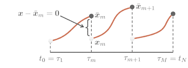
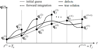
The most important issue with shooting methods is that the condition number of the Jacobian matrix $\Phi(t)$ in the variational equation (6.2.10) typically grows exponentially as $t \rightarrow \infty$. This can result in extremely ill-conditioned equations to solve for the starting point. We can avoid this extreme ill-conditioning by sub-dividing the interval $[a, b]$ into smaller pieces $a=t_0<t_1<\cdots<t_m=b$. Then to solve $g(\boldsymbol{x}(a), \boldsymbol{x}(b))=\mathbf{0}$ where $d \boldsymbol{x} / d t=\boldsymbol{f}(t, \boldsymbol{x})$ we now have additional equations to satisfy so that $\boldsymbol{x}\left(t_j^{+}\right)=\boldsymbol{x}\left(t_j^{-}\right)$at every interior break point $t_j, j=1,2, \ldots, m-1$. We have the functions $\boldsymbol{S}j\left(\boldsymbol{x}_j\right)=z\left(t{j+1}\right)$ where $d z / d t=\boldsymbol{f}(t, z(t))$ and $z\left(t_j\right)=\boldsymbol{x}j$. As for the standard shooting algorithm, $\nabla \boldsymbol{S}_j\left(\boldsymbol{x}_j\right)$ can be computed by means of the variational equation (6.2.10) except that $\nabla \boldsymbol{S}_j\left(\boldsymbol{x}_j\right)=\Phi_j\left(t{j+1}\right)$ where $\Phi_j\left(t_j\right)=I$. Provided we make $L\left|t_{j+1}-t_j\right|$ modest, the condition number of each $\Phi\left(t_{j+1}\right)$ should also be modest, and the overall system should not be ill-conditioned. The overall linear system to be solved for each step of Newton’s method for solving $g(x(a), \boldsymbol{x}(b))=\mathbf{0}$ is Ill-conditioning can still occur, but then it will be inherent in the problem, not an artifact of the shooting method. Also, the multiple shooting matrix is relatively sparse, so block-sparse matrix techniques can be used. For example, we can apply a block LU factorization to the matrix in (6.2.12), utilizing the block sparsity of the matrix. If $x(t) \in \mathbb{R}^n$ then (6.2.12) can be solved in $\mathcal{O}\left(m n^3\right)$ operations. Of course, LU factorization without pivoting can be numerically unstable. On the other hand, a block QR factorization can be performed in $\mathcal{O}\left(m n^3\right)$ operations without the risk of numerical instability, and the block sparsity of the matrix is still preserved.
数值分析代考
数学代写|数值分析代写numerical analysis代考|Shooting Methods
拍摄方法旨在使用解图 $S: x(a) \mapsto \boldsymbol{x}(b)$ 微分方程 $d \boldsymbol{x} / d t=\boldsymbol{f}(t, \boldsymbol{x})$ 帮助解决问题。方程式 $0=$ $\boldsymbol{g}(\boldsymbol{x}(a), \boldsymbol{x}(b))$ 可以写成 $0=\boldsymbol{g}(\boldsymbol{x}(a), \boldsymbol{S}(\boldsymbol{x}(a)))$. 例如,为此我们可以使用牛顿法。这需要计算雅可比 矩阵的估计值
$$
\nabla_{\boldsymbol{x}(a)}[\boldsymbol{g}(\boldsymbol{x}(a), \boldsymbol{S}(\boldsymbol{x}(a)))]=\nabla_{\boldsymbol{x} 1} \boldsymbol{g}(\boldsymbol{x}(a), \boldsymbol{S}(\boldsymbol{x}(a)))+\nabla \boldsymbol{x} 2 \boldsymbol{g}(\boldsymbol{x}(a), \boldsymbol{S}(\boldsymbol{x}(a))) \nabla \boldsymbol{S}(\boldsymbol{x}(a))
$$
我们需要确定 $\nabla \boldsymbol{S}(\boldsymbol{x}(a))$. 让 $\boldsymbol{x}\left(t ; \boldsymbol{x}0\right)$ 是微分方程的解 $d x / d t=f(t, x)$ 和 $\boldsymbol{x}(a)=x_0$. 如果 $\Phi(t)=\nabla x_0 \boldsymbol{x}\left(t ; x_0\right)$ 然后 $$ \frac{d}{d t} \Phi(t)=\frac{d}{d t} \nabla{x_0} x\left(t ; x_0\right)=\nabla_{x_0} \frac{d}{d t} x\left(t ; x_0\right) \quad=\nabla_{x_0}\left[f\left(t, x\left(t ; x_0\right)\right)\right]=\nabla_x f\left(t, x\left(t ; x_0\right)\right)
$$
这是微分方程的变分方程 $d x d t=f(t, \boldsymbol{x})$. 对于初始条件 $\Phi$, 我们注意到 $\boldsymbol{x}(a ; \boldsymbol{x} 0)=\boldsymbol{x}_0$. 所以 $\Phi(a)=\nabla x_0 \boldsymbol{x}(a ; \boldsymbol{x} 0)=\nabla x_0 x_0=I$. 然后 $x(t)$ 和 $\Phi(t)$ 可以使用应用到的标准数值 ODE 求解器一 起计十算
$$
\frac{d}{d t}[x \Phi]=\left[f(t, x) \nabla_x f(t, x) \Phi\right], \quad[x(a) \Phi(a)]=\left[x_0 I\right]
$$
这确实需要计算雅可比矩阵 $\boldsymbol{f}(t, \boldsymbol{x})$ 关于 $\boldsymbol{x}$. 这可以使用符号计算、数值微分公式(参见第 5.5.1.1 节) 或 自动微分 (参见第 5.5 .2 节) 来完成。
一次 $\Phi(t)$ 已被计算, $\nabla \boldsymbol{S}\left(\boldsymbol{x}_0\right)=\Phi(b)$ ,我们可以应用牛顿法。
数学代写|数值分析代写numerical analysis代考|Multiple Shooting
射击方法最重要的问题是雅可比矩阵的条件数 $\Phi(t)$ 在变分方程 (6.2.10) 中,通常呈指数增长 $t \rightarrow \infty$. 这 可能会导致极度病态的方程式求解起点。我们可以通过细分间隔来避免这种极端的病态 $[a, b]$ 分成小块 $a=t_0<t_1<\cdots<t_m=b$. 然后去解决 $g(\boldsymbol{x}(a), \boldsymbol{x}(b))=\mathbf{0}$ 在哪里 $d \boldsymbol{x} / d t=\boldsymbol{f}(t, \boldsymbol{x})$ 我们现在有 额外的方程来满足 $\boldsymbol{x}\left(t_j^{+}\right)=\boldsymbol{x}\left(t_j^{-}\right)$在每个内部断点 $t_j, j=1,2, \ldots, m-1$. 我们有功能 $\boldsymbol{S} j\left(\boldsymbol{x}j\right)=z(t j+1)$ 在哪里 $d z / d t=\boldsymbol{f}(t, z(t))$ 和 $z\left(t_j\right)=\boldsymbol{x} j$. 至于标准的拍摄算法, $\nabla \boldsymbol{S}_j\left(\boldsymbol{x}_j\right)$ 可 以通过变分方程 (6.2.10) 计算,除了 $\nabla \boldsymbol{S}_j\left(\boldsymbol{x}_j\right)=\Phi_j(t j+1)$ 在哪里 $\Phi_j\left(t_j\right)=I$. 只要我们让 $L\left|t{j+1}-t_j\right|$ 谦虚,每个的条件数 $\Phi\left(t_{j+1}\right)$ 也要适度,整体系统不能有病态。牛顿法求解每一步要求解 的整体线性系统 $g(x(a), \boldsymbol{x}(b))=\mathbf{0}$ 就是状态不佳还是会出现,但那会是固有的问题,不是拍摄方法的 人为因素。此外,多重射击矩阵相对稀疏,因此可以使用块稀疏矩阵技术。例如,我们可以利用矩阵的块 稀疏性对 (6.2.12) 中的矩阵应用块 $\mathrm{LU}$ 分解。如果 $x(t) \in \mathbb{R}^n$ 那么 (6.2.12) 可以求解 $\mathcal{O}\left(m n^3\right)$ 操作。当 然,没有主元的 LU 分解在数值上可能不稳定。另一方面,块 $\mathrm{QR}$ 分解可以在 $\mathcal{O}\left(m n^3\right)$ 操作没有数值不 稳定的风险,并且矩阵的块稀疏性仍然保留。

统计代写请认准statistics-lab™. statistics-lab™为您的留学生涯保驾护航。
金融工程代写
金融工程是使用数学技术来解决金融问题。金融工程使用计算机科学、统计学、经济学和应用数学领域的工具和知识来解决当前的金融问题,以及设计新的和创新的金融产品。
非参数统计代写
非参数统计指的是一种统计方法,其中不假设数据来自于由少数参数决定的规定模型;这种模型的例子包括正态分布模型和线性回归模型。
广义线性模型代考
广义线性模型(GLM)归属统计学领域,是一种应用灵活的线性回归模型。该模型允许因变量的偏差分布有除了正态分布之外的其它分布。
术语 广义线性模型(GLM)通常是指给定连续和/或分类预测因素的连续响应变量的常规线性回归模型。它包括多元线性回归,以及方差分析和方差分析(仅含固定效应)。
有限元方法代写
有限元方法(FEM)是一种流行的方法,用于数值解决工程和数学建模中出现的微分方程。典型的问题领域包括结构分析、传热、流体流动、质量运输和电磁势等传统领域。
有限元是一种通用的数值方法,用于解决两个或三个空间变量的偏微分方程(即一些边界值问题)。为了解决一个问题,有限元将一个大系统细分为更小、更简单的部分,称为有限元。这是通过在空间维度上的特定空间离散化来实现的,它是通过构建对象的网格来实现的:用于求解的数值域,它有有限数量的点。边界值问题的有限元方法表述最终导致一个代数方程组。该方法在域上对未知函数进行逼近。[1] 然后将模拟这些有限元的简单方程组合成一个更大的方程系统,以模拟整个问题。然后,有限元通过变化微积分使相关的误差函数最小化来逼近一个解决方案。
tatistics-lab作为专业的留学生服务机构,多年来已为美国、英国、加拿大、澳洲等留学热门地的学生提供专业的学术服务,包括但不限于Essay代写,Assignment代写,Dissertation代写,Report代写,小组作业代写,Proposal代写,Paper代写,Presentation代写,计算机作业代写,论文修改和润色,网课代做,exam代考等等。写作范围涵盖高中,本科,研究生等海外留学全阶段,辐射金融,经济学,会计学,审计学,管理学等全球99%专业科目。写作团队既有专业英语母语作者,也有海外名校硕博留学生,每位写作老师都拥有过硬的语言能力,专业的学科背景和学术写作经验。我们承诺100%原创,100%专业,100%准时,100%满意。
随机分析代写
随机微积分是数学的一个分支,对随机过程进行操作。它允许为随机过程的积分定义一个关于随机过程的一致的积分理论。这个领域是由日本数学家伊藤清在第二次世界大战期间创建并开始的。
时间序列分析代写
随机过程,是依赖于参数的一组随机变量的全体,参数通常是时间。 随机变量是随机现象的数量表现,其时间序列是一组按照时间发生先后顺序进行排列的数据点序列。通常一组时间序列的时间间隔为一恒定值(如1秒,5分钟,12小时,7天,1年),因此时间序列可以作为离散时间数据进行分析处理。研究时间序列数据的意义在于现实中,往往需要研究某个事物其随时间发展变化的规律。这就需要通过研究该事物过去发展的历史记录,以得到其自身发展的规律。
回归分析代写
多元回归分析渐进(Multiple Regression Analysis Asymptotics)属于计量经济学领域,主要是一种数学上的统计分析方法,可以分析复杂情况下各影响因素的数学关系,在自然科学、社会和经济学等多个领域内应用广泛。
MATLAB代写
MATLAB 是一种用于技术计算的高性能语言。它将计算、可视化和编程集成在一个易于使用的环境中,其中问题和解决方案以熟悉的数学符号表示。典型用途包括:数学和计算算法开发建模、仿真和原型制作数据分析、探索和可视化科学和工程图形应用程序开发,包括图形用户界面构建MATLAB 是一个交互式系统,其基本数据元素是一个不需要维度的数组。这使您可以解决许多技术计算问题,尤其是那些具有矩阵和向量公式的问题,而只需用 C 或 Fortran 等标量非交互式语言编写程序所需的时间的一小部分。MATLAB 名称代表矩阵实验室。MATLAB 最初的编写目的是提供对由 LINPACK 和 EISPACK 项目开发的矩阵软件的轻松访问,这两个项目共同代表了矩阵计算软件的最新技术。MATLAB 经过多年的发展,得到了许多用户的投入。在大学环境中,它是数学、工程和科学入门和高级课程的标准教学工具。在工业领域,MATLAB 是高效研究、开发和分析的首选工具。MATLAB 具有一系列称为工具箱的特定于应用程序的解决方案。对于大多数 MATLAB 用户来说非常重要,工具箱允许您学习和应用专业技术。工具箱是 MATLAB 函数(M 文件)的综合集合,可扩展 MATLAB 环境以解决特定类别的问题。可用工具箱的领域包括信号处理、控制系统、神经网络、模糊逻辑、小波、仿真等。