
如果你也在 怎样代写回归分析Regression Analysis 这个学科遇到相关的难题,请随时右上角联系我们的24/7代写客服。回归分析Regression Analysis回归中的概率观点具体体现在给定X数据的特定固定值的Y数据的可变性模型中。这种可变性是用条件分布建模的;因此,副标题是:“条件分布方法”。回归的整个主题都是用条件分布来表达的;这种观点统一了不同的方法,如经典回归、方差分析、泊松回归、逻辑回归、异方差回归、分位数回归、名义Y数据模型、因果模型、神经网络回归和树回归。所有这些都可以方便地用给定特定X值的Y条件分布模型来看待。
回归分析Regression Analysis条件分布是回归数据的正确模型。它们告诉你,对于变量X的给定值,可能存在可观察到的变量Y的分布。如果你碰巧知道这个分布,那么你就知道了你可能知道的关于响应变量Y的所有信息,因为它与预测变量X的给定值有关。与基于R^2统计量的典型回归方法不同,该模型解释了100%的潜在可观察到的Y数据,后者只解释了Y数据的一小部分,而且在假设几乎总是被违反的情况下也是不正确的。
statistics-lab™ 为您的留学生涯保驾护航 在代写回归分析Regression Analysis方面已经树立了自己的口碑, 保证靠谱, 高质且原创的统计Statistics代写服务。我们的专家在代写回归分析Regression Analysis代写方面经验极为丰富,各种代写回归分析Regression Analysis相关的作业也就用不着说。
统计代写|回归分析作业代写Regression Analysis代考|Multiple Regression from the Matrix Point of View
In the case of simple regression, you saw that the OLS estimate of slope has a simple form: It is the estimated covariance of the $(X, Y)$ distribution, divided by the estimated variance of the $X$ distribution, or $\hat{\beta}1=\hat{\sigma}{x y} / \hat{\sigma}_x^2$. There is no such simple formula in multiple regression. Instead, you must use matrix algebra, involving matrix multiplication and matrix inverses. If you are unfamiliar with basic matrix algebra, including multiplication, addition, subtraction, transpose, identity matrix, and matrix inverse, you should take some time now to get acquainted with those particular concepts before reading on. (Perhaps you can locate a “matrix algebra for beginners” type of web page.)
Done? Ok, read on.
Our first use of matrix algebra in regression is to give a concise representation of the regression model. Multiple regression models refer to $n$ observations and $k$ variables, both of which can be in the thousands or even millions. The following matrix form of the model provides a very convenient shorthand to represent all this information.
$$
Y=\mathrm{X} \beta+\varepsilon
$$
This concise form covers all the $n$ observations and all the $X$ variables ( $k$ of them) in one simple equation. Note that there are boldface non-italic terms and boldface italic terms in the expression. To make the material easier to read, we use the convention that boldface means a matrix, while boldface italic refers to a vector, which is a matrix with a single column. Thus $\boldsymbol{Y}, \boldsymbol{\beta}$, and $\varepsilon$, are vectors (single-column matrices), while $\mathbf{X}$ is a matrix having multiple columns.
统计代写|回归分析作业代写Regression Analysis代考|The Least Squares Estimates in Matrix Form
One use of matrix algebra is to display the model for all $n$ observations and all $X$ variables succinctly as shown above. Another use is to identify the OLS estimates of the $\beta$ ‘s. There is simply no way to display the OLS estimates other than by using matrix algebra, as follows:
$$
\hat{\boldsymbol{\beta}}=\left(\mathbf{X}^{\mathrm{T}} \mathbf{X}\right)^{-1} \mathbf{X}^{\mathrm{T}} Y
$$
(The ” $\mathrm{T}$ ” symbol denotes transpose of the matrix.) To see why the OLS estimates have this matrix representation, recall that in the simple, classical regression model, the maximum likelihood (ML) estimates must minimize the sum of squared “errors” called SSE. The same is true in multiple regression: The ML estimates must minimize the function
$$
\operatorname{SSE}\left(\beta_0, \beta_1, \ldots, \beta_k\right)=\sum_{i=1}^n\left{y_i-\left(\beta_0+\beta_1 x_{i 1}+\cdots+\beta_k x_{i k}\right)\right}^2
$$
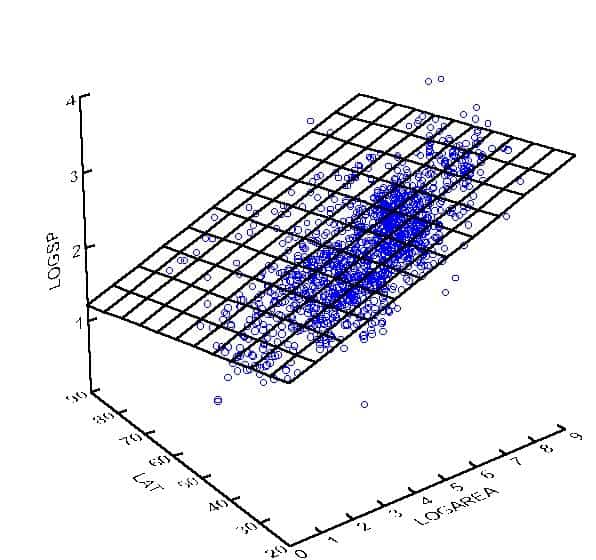
In the case of two $X$ variables $(k=2)$, you are to choose $\hat{\beta}0, \hat{\beta}_1$, and $\hat{\beta}_2$ that define the plane, $f\left(x_1, x_2\right)=\hat{\beta}_0+\hat{\beta}_1 x_1+\hat{\beta}_2 x_2$, such as the one shown in Figure 6.3 , that minimizes the sum of squared vertical deviations from the 3-dimensional point cloud $\left(x{i 1}, x_{i 2}, y_i\right), i=1,2, \ldots, n$. Figure 7.1 illustrates the concept.
回归分析代写
统计代写|回归分析作业代写Regression Analysis代考|Multiple Regression from the Matrix Point of View
在简单回归的情况下,您看到斜率的OLS估计有一个简单的形式:它是$(X, Y)$分布的估计协方差除以$X$分布或$\hat{\beta}1=\hat{\sigma}{x y} / \hat{\sigma}_x^2$的估计方差。在多元回归中没有这样简单的公式。相反,你必须使用矩阵代数,包括矩阵乘法和矩阵逆。如果您不熟悉基本的矩阵代数,包括乘法、加法、减法、转置、单位矩阵和矩阵逆,那么在继续阅读之前,您应该花一些时间熟悉这些特定的概念。(也许你可以找到一个“矩阵代数初学者”类型的网页。)
搞定了?好吧,继续读下去。
我们在回归中首先使用矩阵代数是为了给出回归模型的简明表示。多元回归模型涉及$n$观测值和$k$变量,这两个变量都可以是数千甚至数百万。该模型的以下矩阵形式提供了一种非常方便的速记方式来表示所有这些信息。
$$
Y=\mathrm{X} \beta+\varepsilon
$$
这个简洁的形式在一个简单的方程中涵盖了所有的$n$观测值和所有的$X$变量(其中的$k$变量)。请注意,表达式中有黑体非斜体项和黑体斜体项。为了使材料更容易阅读,我们使用约定,黑体表示矩阵,而黑体斜体表示向量,这是一个具有单列的矩阵。因此$\boldsymbol{Y}, \boldsymbol{\beta}$和$\varepsilon$是向量(单列矩阵),而$\mathbf{X}$是具有多列的矩阵。
统计代写|回归分析作业代写Regression Analysis代考|The Least Squares Estimates in Matrix Form
矩阵代数的一种用法是简洁地显示所有$n$观测值和所有$X$变量的模型,如上所示。另一个用途是识别$\beta$的OLS估计。除了使用矩阵代数之外,根本没有办法显示OLS估计,如下所示:
$$
\hat{\boldsymbol{\beta}}=\left(\mathbf{X}^{\mathrm{T}} \mathbf{X}\right)^{-1} \mathbf{X}^{\mathrm{T}} Y
$$
(“$\mathrm{T}$”符号表示矩阵的转置。)要了解为什么OLS估计具有这种矩阵表示,请回忆一下,在简单的经典回归模型中,最大似然(ML)估计必须最小化称为SSE的平方“误差”的总和。在多元回归中也是如此:机器学习估计必须最小化函数
$$
\operatorname{SSE}\left(\beta_0, \beta_1, \ldots, \beta_k\right)=\sum_{i=1}^n\left{y_i-\left(\beta_0+\beta_1 x_{i 1}+\cdots+\beta_k x_{i k}\right)\right}^2
$$
在有两个$X$变量$(k=2)$的情况下,您将选择$\hat{\beta}0, \hat{\beta}1$和$\hat{\beta}_2$来定义平面$f\left(x_1, x_2\right)=\hat{\beta}_0+\hat{\beta}_1 x_1+\hat{\beta}_2 x_2$,如图6.3所示,它最小化与三维点云$\left(x{i 1}, x{i 2}, y_i\right), i=1,2, \ldots, n$垂直偏差的平方和。图7.1说明了这个概念。

统计代写请认准statistics-lab™. statistics-lab™为您的留学生涯保驾护航。