如果你也在 怎样代写统计力学Statistical mechanics这个学科遇到相关的难题,请随时右上角联系我们的24/7代写客服。
统计力学是一个数学框架,它将统计方法和概率理论应用于大型微观实体的集合。它不假设或假定任何自然法则,而是从这种集合体的行为来解释自然界的宏观行为。
statistics-lab™ 为您的留学生涯保驾护航 在代写统计力学Statistical mechanics方面已经树立了自己的口碑, 保证靠谱, 高质且原创的统计Statistics代写服务。我们的专家在代写统计力学Statistical mechanics代写方面经验极为丰富,各种代写统计力学Statistical mechanics相关的作业也就用不着说。
我们提供的统计力学Statistical mechanics及其相关学科的代写,服务范围广, 其中包括但不限于:
- Statistical Inference 统计推断
- Statistical Computing 统计计算
- Advanced Probability Theory 高等概率论
- Advanced Mathematical Statistics 高等数理统计学
- (Generalized) Linear Models 广义线性模型
- Statistical Machine Learning 统计机器学习
- Longitudinal Data Analysis 纵向数据分析
- Foundations of Data Science 数据科学基础
物理代写|统计力学代写Statistical mechanics代考|Wave packets as eigenfunctions in the classical limit
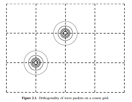
The primary goal here is to show how to get from the quantum picture to classical statistical mechanics, which is of course formulated in the classical phase space of the particles’ positions and momenta. To this end we use wave packets because they are localized simultaneously in position and momentum. Some care must be taken with using these as a basis, as there are issues with their orthogonality and completeness. Also the meaning of simultaneous localization must be reconciled with the Heisenberg uncertainty principle.
Consider a system consisting of $N$ particles in three dimensions, with position representation coordinates $\mathbf{r}=\left{\mathbf{r}{1}, \mathbf{r}{2}, \ldots, \mathbf{r}{N}\right}, \mathbf{r}{j}=\left{r_{j x}, r_{j y}, r_{j z}\right}, j=1,2, \ldots, N$. Define analogous vectors for the position label $\mathbf{q}$, and the momentum label $\mathbf{p}$. It will sometimes be convenient to write the combined labels as $\mathbf{\Gamma} \equiv{\mathbf{q}, \mathbf{p}}$. The representation coordinates $\mathbf{r}$ belong to the real continuum. The labels are discretized, for example $q_{j \alpha}=\ell_{\mathrm{q}, j \alpha} \Delta_{\mathrm{q}}$ and $p_{j a}=\ell_{\mathrm{p}, j \alpha} \Delta_{\mathrm{p}}$, with the $\ell_{\mathrm{q}}$ and $\ell_{\mathrm{p}}$ being integers. Below $\Gamma$ and $\ell$ are used interchangeably to label the system state. The meaning of position and momentum labels emerges from the following analysis.
At this stage we do not need to be more precise about the grid spacing or the system size. Messiah (1961, chapter V, section 11) insists that in order for the momentum operator to be Hermitian periodic boundary conditions must be imposed on all wave functions, and discrete momentum eigenvalues must have spacing $\Delta_{\mathrm{p}}=2 \pi \hbar / L$ where $I$. is the system edge length. This is true if the wave function does not go to zero at the boundaries. In any case, here we do not explicitly use this (but we consistently do so in later chapters), but instead observe that for a macroscopic system, $L \rightarrow \infty$, the present grid spacing could be made an integer multiple of this.
Spin could be included in the set of commuting dynamical variables, with $\mathbf{x}{j}=\left{\mathbf{r}{j}, \sigma_{j}\right}$, where $\sigma_{j} \in{-S,-S+1, \ldots, S}$ is the $z$-component of the spin of particle j. See Messiah (1961, section 14.1), or Merzbacher (1970, section 20.5), or section $6.4$ below. However, we do not include spin in the present analysis.
物理代写|统计力学代写Statistical mechanics代考| Eigenfunctions
The probability amplitude in the position representation is
$$
\zeta_{\mathrm{q}, \mathrm{p}}(\mathbf{r})^{*} \zeta_{\mathrm{q}, \mathrm{p}}(\mathbf{r})=\frac{1}{C^{2}} e^{-(\mathbf{r}-\mathbf{q})(\mathbf{r}-\mathbf{q}) / 2 \xi^{2}} .
$$
This is a Gaussian of width $\xi$ (per particle, per direction), peaked at the position label $\mathbf{q}$. Similarly in the momentum representation, the probability amplitude has width $\hbar / 2 \xi$ and is peaked at the momentum label p. To within an error of these magnitudes, the minimum uncertainty wave function is approximately a simultaneous eigenfunction of the position and momentum operators,
$$
\hat{\mathbf{q}} \zeta_{\mathbf{q}, \mathbf{p}}(\mathbf{r})=\mathbf{r} \zeta_{\mathbf{q}, \mathrm{p}}(\mathbf{r}) \approx \mathbf{q} \zeta_{\mathbf{q}, \mathbf{p}}(\mathbf{r}),
$$
and
$$
\hat{\mathbf{p}} \zeta_{\mathrm{q}, \mathrm{p}}(\mathbf{r})=\left[\frac{\mathrm{i} \hbar}{2 \xi^{2}}(\mathbf{r}-\mathbf{q})+\mathbf{p}\right] \zeta_{\mathrm{q}, \mathrm{p}}(\mathbf{r}) \approx \mathbf{p} \zeta_{\mathrm{q}, \mathrm{p}}(\mathbf{r}) .
$$
(Recall that the momentum operator is $\hat{\mathbf{p}}=-i \hbar \nabla_{\mathbf{r}}$.) Since the probability amplitude is sharply peaked about ${\mathbf{q}, \mathbf{p}}$, the approximation in these is to neglect contributions $\mathcal{O}(\xi)$ and $\mathcal{O}(\hbar / 2 \xi)$, respectively.
Because the wave packet is an approximate simultaneous position and momentum eigenfunction, for any sufficiently slowly varying phase function one can write $\int(\hat{\mathbf{q}}, \hat{\mathbf{p}}) \zeta_{\mathbf{q}, \mathbf{p}}(\mathbf{r}) \approx f(\mathbf{q}, \mathbf{p}) \zeta_{\mathbf{q}, \mathbf{p}}(\mathbf{r})$. In particular, the wave packet is an approximate energy eigenfunction,
$$
\hat{H}(\mathbf{r}) \zeta_{\mathbf{q}, \mathbf{p}}(\mathbf{r}) \equiv H(\hat{\mathbf{q}}, \hat{\mathbf{p}}) \zeta_{\mathbf{q}, \mathbf{p}}(\mathbf{r}) \approx H(\mathbf{q}, \mathbf{p}) \zeta_{\mathbf{q}, \mathbf{p}}(\mathbf{r}) .
$$
The eigenvalue is the classical Hamiltonian energy function of phase space, which is usually split into kinetic and potential energies,
$$
H(\mathbf{q}, \mathbf{p})=\mathcal{K}(\mathbf{p})+U(\mathbf{q}), \quad \mathcal{K}(\mathbf{p})=\frac{p^{2}}{2 m}=\frac{1}{2 m} \sum_{j, \alpha} p_{j \alpha}^{2} .
$$
统计力学代考
物理代写|统计力学代写Statistical mechanics代考|Wave packets as eigenfunctions in the classical limit
这里的主要目标是展示如何从量子图像到经典统计力学,这当然是在粒子位置和动量的经典相空间中制定的。为 此,我们使用波包,因为它们同时定位在位置和动量上。使用这些作为基础时必须小心谨慎,因为它们的正交性 和完整性存在问题。同时定位的含义也必须与海森堡测不准原理相协调。
考虑一个由以下组成的系统 $N$ 三个维度的粒子,具有位置表示坐标 . 为位置标签定义类似向量 $\mathbf{q}$, 和动量标签 $\mathbf{p}$. 有时将组合标签写为 $\boldsymbol{\Gamma} \equiv \mathbf{q}, \mathbf{p}$. 表示坐标 $\mathbf{r}$ 属于实相。标签是离散
的,例如 $q_{j \alpha}=\ell_{\mathrm{q}, j \alpha} \Delta_{\mathrm{q}}$ 和 $p_{j a}=\ell_{\mathrm{p}, j \alpha} \Delta_{\mathrm{p}}$, 与 $\ell_{\mathrm{q}}$ 和 $\ell_{\mathrm{p}}$ 是整数。以下 $\Gamma$ 和 $\ell$ 可以互换使用来标记系统状态。位置和 动量标签的含义来自以下分析。
在这个阶段,我们不需要更精确的网格间距或系统大小。Messiah(1961 年,第五章,第 11 节) 坚持认为,为 了使动量算子成为厄米特周期边界条件,必须对所有波函数施加周期性边界条件,并且离散动量特征值必须具有 间距 $\Delta_{\mathrm{p}}=2 \pi \hbar / L$ 在哪里 $I$. 是系统边长。如果波函数在边界处不为零,这是正确的。无论如何,这里我们没有 明确地使用它(但我们在后面的章节中一直这样做),而是观察到对于宏观系统, $L \rightarrow \infty$ ,现在的网格间距可 以是这个的整数倍。 $\sigma_{j} \in-S,-S+1, \ldots, S$ 是个 $z$-粒子 $\mathrm{j}$ 的自旋分量。见 Messiah (1961, section 14.1), or Merzbacher (1970, section 20.5), or section6.4以下。但是,我们在本分析中不包括自旋。
物理代写|统计力学代写Statistical mechanics代考| Eigenfunctions
位置表示中的概率幅度为
$$
\zeta_{\mathrm{q}, \mathrm{p}}(\mathbf{r})^{*} \zeta_{\mathrm{q}, \mathrm{p}}(\mathbf{r})=\frac{1}{C^{2}} e^{-(\mathbf{r}-\mathbf{q})(\mathbf{r}-\mathbf{q}) / 2 \xi^{2}}
$$
这是宽度的高斯 $\xi$ (每个粒子,每个方向),在位置标签处达到峰值q. 类似地,在动量表示中,概率幅具有宽度 $\hbar / 2 \xi$ 并且在动量标签 $\mathrm{p}$ 处达到峰值。在这些量级的误差范围内,最小不确定性波函数近似为位置和动量算子的同 时特征函数,
$$
\hat{\mathbf{q}} \zeta_{\mathbf{q}, \mathbf{p}}(\mathbf{r})=\mathbf{r} \zeta_{\mathbf{q}, \mathbf{p}}(\mathbf{r}) \approx \mathbf{q} \zeta_{\mathbf{q}, \mathbf{p}}(\mathbf{r})
$$
和
$$
\hat{\mathbf{p}} \zeta_{\mathrm{q}, \mathrm{p}}(\mathbf{r})=\left[\frac{\mathrm{i} \hbar}{2 \xi^{2}}(\mathbf{r}-\mathbf{q})+\mathbf{p}\right] \zeta_{\mathrm{q}, \mathrm{p}}(\mathbf{r}) \approx \mathbf{p} \zeta_{\mathrm{q}, \mathrm{p}}(\mathbf{r})
$$
(回想一下,动量算子是 $\hat{\mathbf{p}}=-i \hbar \nabla_{\mathbf{r}}$.) 由于概率幅度在大约 $\mathbf{q}, \mathbf{p}$ ,其中的近似值是忽略贡献 $\mathcal{O}(\xi)$ 和 $\mathcal{O}(\hbar / 2 \xi)$ ,分别。
因为波包是一个近似的同时位置和动量特征函数,对于任何足够缓慢变化的相位函数,我们可以写出 $\int(\hat{\mathbf{q}}, \hat{\mathbf{p}}) \zeta_{\mathbf{q}, \mathbf{p}}(\mathbf{r}) \approx f(\mathbf{q}, \mathbf{p}) \zeta_{\mathbf{q}, \mathbf{p}}(\mathbf{r})$. 特别地,波包是一个近似的能量特征函数,
$$
\hat{H}(\mathbf{r}) \zeta_{\mathbf{q}, \mathbf{p}}(\mathbf{r}) \equiv H(\hat{\mathbf{q}}, \hat{\mathbf{p}}) \zeta_{\mathbf{q}, \mathbf{p}}(\mathbf{r}) \approx H(\mathbf{q}, \mathbf{p}) \zeta_{\mathbf{q}, \mathbf{p}}(\mathbf{r})
$$
特征值是相空间的经典哈密顿能量函数,通常分为动能和势能,
$$
H(\mathbf{q}, \mathbf{p})=\mathcal{K}(\mathbf{p})+U(\mathbf{q}), \quad \mathcal{K}(\mathbf{p})=\frac{p^{2}}{2 m}=\frac{1}{2 m} \sum_{j, \alpha} p_{j \alpha}^{2}
$$

统计代写请认准statistics-lab™. statistics-lab™为您的留学生涯保驾护航。
金融工程代写
金融工程是使用数学技术来解决金融问题。金融工程使用计算机科学、统计学、经济学和应用数学领域的工具和知识来解决当前的金融问题,以及设计新的和创新的金融产品。
非参数统计代写
非参数统计指的是一种统计方法,其中不假设数据来自于由少数参数决定的规定模型;这种模型的例子包括正态分布模型和线性回归模型。
广义线性模型代考
广义线性模型(GLM)归属统计学领域,是一种应用灵活的线性回归模型。该模型允许因变量的偏差分布有除了正态分布之外的其它分布。
术语 广义线性模型(GLM)通常是指给定连续和/或分类预测因素的连续响应变量的常规线性回归模型。它包括多元线性回归,以及方差分析和方差分析(仅含固定效应)。
有限元方法代写
有限元方法(FEM)是一种流行的方法,用于数值解决工程和数学建模中出现的微分方程。典型的问题领域包括结构分析、传热、流体流动、质量运输和电磁势等传统领域。
有限元是一种通用的数值方法,用于解决两个或三个空间变量的偏微分方程(即一些边界值问题)。为了解决一个问题,有限元将一个大系统细分为更小、更简单的部分,称为有限元。这是通过在空间维度上的特定空间离散化来实现的,它是通过构建对象的网格来实现的:用于求解的数值域,它有有限数量的点。边界值问题的有限元方法表述最终导致一个代数方程组。该方法在域上对未知函数进行逼近。[1] 然后将模拟这些有限元的简单方程组合成一个更大的方程系统,以模拟整个问题。然后,有限元通过变化微积分使相关的误差函数最小化来逼近一个解决方案。
tatistics-lab作为专业的留学生服务机构,多年来已为美国、英国、加拿大、澳洲等留学热门地的学生提供专业的学术服务,包括但不限于Essay代写,Assignment代写,Dissertation代写,Report代写,小组作业代写,Proposal代写,Paper代写,Presentation代写,计算机作业代写,论文修改和润色,网课代做,exam代考等等。写作范围涵盖高中,本科,研究生等海外留学全阶段,辐射金融,经济学,会计学,审计学,管理学等全球99%专业科目。写作团队既有专业英语母语作者,也有海外名校硕博留学生,每位写作老师都拥有过硬的语言能力,专业的学科背景和学术写作经验。我们承诺100%原创,100%专业,100%准时,100%满意。
随机分析代写
随机微积分是数学的一个分支,对随机过程进行操作。它允许为随机过程的积分定义一个关于随机过程的一致的积分理论。这个领域是由日本数学家伊藤清在第二次世界大战期间创建并开始的。
时间序列分析代写
随机过程,是依赖于参数的一组随机变量的全体,参数通常是时间。 随机变量是随机现象的数量表现,其时间序列是一组按照时间发生先后顺序进行排列的数据点序列。通常一组时间序列的时间间隔为一恒定值(如1秒,5分钟,12小时,7天,1年),因此时间序列可以作为离散时间数据进行分析处理。研究时间序列数据的意义在于现实中,往往需要研究某个事物其随时间发展变化的规律。这就需要通过研究该事物过去发展的历史记录,以得到其自身发展的规律。
回归分析代写
多元回归分析渐进(Multiple Regression Analysis Asymptotics)属于计量经济学领域,主要是一种数学上的统计分析方法,可以分析复杂情况下各影响因素的数学关系,在自然科学、社会和经济学等多个领域内应用广泛。
MATLAB代写
MATLAB 是一种用于技术计算的高性能语言。它将计算、可视化和编程集成在一个易于使用的环境中,其中问题和解决方案以熟悉的数学符号表示。典型用途包括:数学和计算算法开发建模、仿真和原型制作数据分析、探索和可视化科学和工程图形应用程序开发,包括图形用户界面构建MATLAB 是一个交互式系统,其基本数据元素是一个不需要维度的数组。这使您可以解决许多技术计算问题,尤其是那些具有矩阵和向量公式的问题,而只需用 C 或 Fortran 等标量非交互式语言编写程序所需的时间的一小部分。MATLAB 名称代表矩阵实验室。MATLAB 最初的编写目的是提供对由 LINPACK 和 EISPACK 项目开发的矩阵软件的轻松访问,这两个项目共同代表了矩阵计算软件的最新技术。MATLAB 经过多年的发展,得到了许多用户的投入。在大学环境中,它是数学、工程和科学入门和高级课程的标准教学工具。在工业领域,MATLAB 是高效研究、开发和分析的首选工具。MATLAB 具有一系列称为工具箱的特定于应用程序的解决方案。对于大多数 MATLAB 用户来说非常重要,工具箱允许您学习和应用专业技术。工具箱是 MATLAB 函数(M 文件)的综合集合,可扩展 MATLAB 环境以解决特定类别的问题。可用工具箱的领域包括信号处理、控制系统、神经网络、模糊逻辑、小波、仿真等。