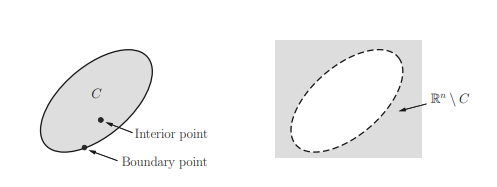
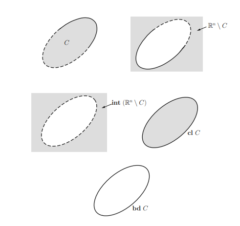
数学代写|凸优化作业代写Convex Optimization代考|Examples of convex sets
如果你也在 怎样代写凸优化Convex Optimization这个学科遇到相关的难题,请随时右上角联系我们的24/7代写客服。
凸优化是数学优化的一个子领域,研究的是凸集上凸函数最小化的问题。许多类凸优化问题都有多项时间算法,而数学优化一般来说是NP困难的。
statistics-lab™ 为您的留学生涯保驾护航 在代写凸优化Convex Optimization方面已经树立了自己的口碑, 保证靠谱, 高质且原创的统计Statistics代写服务。我们的专家在代写凸优化Convex Optimization代写方面经验极为丰富,各种代写凸优化Convex Optimization相关的作业也就用不着说。
我们提供的凸优化Convex Optimization及其相关学科的代写,服务范围广, 其中包括但不限于:
- Statistical Inference 统计推断
- Statistical Computing 统计计算
- Advanced Probability Theory 高等概率论
- Advanced Mathematical Statistics 高等数理统计学
- (Generalized) Linear Models 广义线性模型
- Statistical Machine Learning 统计机器学习
- Longitudinal Data Analysis 纵向数据分析
- Foundations of Data Science 数据科学基础
数学代写|凸优化作业代写Convex Optimization代考|Hyperplanes and halfspaces
A hyperplane is an affine set (hence a convex set) and is of the form
$$
H=\left{\mathbf{x} \mid \mathbf{a}^{T} \mathbf{x}=b\right} \subset \mathbb{R}^{n},
$$
where $\mathbf{a} \in \mathbb{R}^{n} \backslash\left{\mathbf{0}_{n}\right}$ is a normal vector of the hyperplane, and $b \in \mathbb{R}$. Analytically it is the solution set of a linear equation of the components of $\mathbf{x}$. In geometrical sense, a hyperplane can be interpreted as the set of points having a constant inner product (b) with the normal vector (a). Since affdim $(H)=n-1$,
the hyperplane (2.30) can also be expressed as
$$
H=\operatorname{aff}\left{\mathbf{s}{1}, \ldots, \mathbf{s}{n}\right} \subset \mathbb{R}^{n},
$$
where $\left{\mathbf{s}{1}, \ldots, \mathbf{s}{n}\right} \subset H$ is any affinely independent set. Then it can be seen that
$$
\left{\begin{array}{l}
\mathbf{B} \triangleq\left[\mathbf{s}{2}-\mathbf{s}{1}, \ldots, \mathbf{s}{n}-\mathbf{s}{1}\right] \in \mathbb{R}^{n \times(n-1)} \text { and } \operatorname{dim}(\mathcal{R}(\mathbf{B}))=n-1 \
\mathbf{B}^{T} \mathbf{a}=\mathbf{0}{n-1}, \text { i.e. }, \mathcal{R}(\mathbf{B})^{\perp}=\mathcal{R}(\mathbf{a}) \end{array}\right. $$ implying that the normal vector a can be determined from $\left{\mathbf{s}{1}, \ldots, \mathbf{s}_{n}\right}$ up to a scale factor.
The hyperplane $H$ defined in $(2.30)$ divides $\mathbb{R}^{n}$ into two closed halfspaces as follows:
$$
\begin{aligned}
&H_{-}=\left{\mathbf{x} \mid \mathbf{a}^{T} \mathbf{x} \leq b\right} \
&H_{+}=\left{\mathbf{x} \mid \mathbf{a}^{T} \mathbf{x} \geq b\right}
\end{aligned}
$$
and so each of them is the solution set of one (non-trivial) linear inequality. Note that $\mathbf{a}=\nabla\left(\mathbf{a}^{T} \mathbf{x}\right)$ denotes the maximally increasing direction of the linear function $\mathbf{a}^{T} \mathbf{x}$. The above representations for both $H_{-}$and $H_{+}$for a given $\mathbf{a} \neq \mathbf{0}$, are not unique, while they are unique if $\mathbf{a}$ is normalized such that $|\mathbf{a}|_{2}=1$. Moreover, $H_{-} \cap H_{+}=H$.
An open halfspace is a set of the form
$$
H_{–}=\left{\mathbf{x} \mid \mathbf{a}^{T} \mathbf{x}b\right}
$$
where $\mathbf{a} \in \mathbb{R}^{n}, \mathbf{a} \neq \mathbf{0}$, and $b \in \mathbb{R}$.
数学代写|凸优化作业代写Convex Optimization代考|Euclidean balls and ellipsoids
A Euclidean ball (or, simply, ball) in $\mathbb{R}^{n}$ has the following form:
$$
B\left(\mathbf{x}{c}, r\right)=\left{\mathbf{x} \mid\left|\mathbf{x}-\mathbf{x}{c}\right|_{2} \leq r\right}=\left{\mathbf{x} \mid\left(\mathbf{x}-\mathbf{x}{c}\right)^{T}\left(\mathbf{x}-\mathbf{x}{c}\right) \leq r^{2}\right},
$$
where $r>0$. The vector $\mathbf{x}{c}$ is the center of the ball and the positive scalar $r$ is its radius (see Figure 2.7). The Euclidean ball is also a 2-norm ball, and, for simplicity, a ball without explicitly mentioning the associated norm, means the Euclidean ball hereafter. Another common representation for the Euclidean ball is $$ B\left(\mathbf{x}{c}, r\right)=\left{\mathbf{x}{c}+r \mathbf{u} \mid|\mathbf{u}|{2} \leq 1\right}
$$
It can be easily proved that the Euclidean ball is a convex set.
Proof of convexity: Let $\mathbf{x}{1}$ and $\mathbf{x}{2} \in B\left(\mathbf{x}{c}, r\right)$, i.e., $\left|\mathbf{x}{1}-\mathbf{x}{c}\right|{2} \leq r$ and $| \mathbf{x}{2}-$ $\mathbf{x}{c} |_{2} \leq r$. Then,
$$
\begin{aligned}
\left|\theta \mathbf{x}{1}+(1-\theta) \mathbf{x}{2}-\mathbf{x}{c}\right|{2} &=\left|\theta \mathbf{x}{1}+(1-\theta) \mathbf{x}{2}-\left[\theta \mathbf{x}{c}+(1-\theta) \mathbf{x}{c}\right]\right|_{2} \
&=\left|\theta\left(\mathbf{x}{1}-\mathbf{x}{c}\right)+(1-\theta)\left(\mathbf{x}{2}-\mathbf{x}{c}\right)\right|_{2} \
& \leq\left|\theta\left(\mathbf{x}{1}-\mathbf{x}{c}\right)\right|_{2}+\left|(1-\theta)\left(\mathbf{x}{2}-\mathbf{x}{c}\right)\right|_{2} \
& \leq \theta r+(1-\theta) r \
&=r, \text { for all } 0 \leq \theta \leq 1
\end{aligned}
$$
Hence, $\theta \mathbf{x}{1}+(1-\theta) \mathbf{x}{2} \in B\left(\mathbf{x}{c}, r\right)$ for all $\theta \in[0,1]$, and thus we have proven that $B\left(\mathbf{x}{c}, r\right)$ is convex.
A related family of convex sets are ellipsoids (see Figure $2.7$ ), which have the form
$$
\mathcal{E}=\left{\mathbf{x} \mid\left(\mathbf{x}-\mathbf{x}{c}\right)^{T} \mathbf{P}^{-1}\left(\mathbf{x}-\mathbf{x}{c}\right) \leq 1\right},
$$
where $\mathbf{P} \in \mathcal{S}{++}^{n}$ and the vector $\mathbf{x}{c}$ is the center of the ellipsoid. The matrix $\mathbf{P}$ determines how far the ellipsoid extends in every direction from the center; the lengths of the semiaxes of $\mathcal{E}$ are given by $\sqrt{\lambda_{i}}$, where $\lambda_{i}$ are eigenvalues of $\mathbf{P}$. Note that a ball is an ellipsoid with $\mathbf{P}=r^{2} \mathbf{I}{n}$ where $r>0$. Another common representation of an ellipsoid is $$ \mathcal{E}=\left{\mathbf{x}{c}+\mathbf{A u} \mid|\mathbf{u}|_{2} \leq 1\right}
$$
where $\mathbf{A}$ is a square matrix and nonsingular. The ellipsoid $\mathcal{E}$ expressed by (2.38) is actually the image of the 2 -norm ball $B(\mathbf{0}, 1)=\left{\mathbf{u} \in \mathbb{R}^{n} \mid|\mathbf{u}|_{2} \leq 1\right}$ via an
affine mapping $\mathbf{x}{c}+\mathbf{A u}$ (cf. $\left.(2.58)\right)$, where $\mathbf{A}=\left(\mathbf{P}^{1 / 2}\right)^{T}$, and the proof will be presented below. With the expression (2.38) for an ellipsoid, the singular values of $\mathbf{A}, \sigma{i}(\mathbf{A})=\sqrt{\lambda_{i}}$ (lengths of semiaxes) characterize the structure of the ellipsoid in a more straightforward fashion than the expression (2.37).
Proof of the ellipsoid representation (2.38) and convexity: Let
$$
\mathbf{P}=\mathbf{Q} \boldsymbol{\Lambda} \mathbf{Q}^{T}=\left(\mathbf{P}^{1 / 2}\right)^{T} \mathbf{P}^{1 / 2}
$$
$(\mathrm{EVD}$ of $\mathbf{P} \succ \mathbf{0})$, where $\boldsymbol{\Lambda}=\boldsymbol{\operatorname { D i a g }}\left(\lambda_{1}, \lambda_{2}, \ldots, \lambda_{n}\right)$ and
$$
\mathbf{P}^{1 / 2}=\boldsymbol{\Lambda}^{1 / 2} \mathbf{Q}^{T},
$$
in which $\Lambda^{1 / 2}=\operatorname{Diag}\left(\sqrt{\lambda_{1}}, \sqrt{\lambda_{2}}, \ldots, \sqrt{\lambda_{n}}\right)$. Then
$$
\mathbf{P}^{-1}=\mathbf{Q} \boldsymbol{\Lambda}^{-1} \mathbf{Q}^{T}=\mathbf{P}^{-1 / 2}\left(\mathbf{P}^{-1 / 2}\right)^{T}, \quad \mathbf{P}^{-1 / 2}=\mathbf{Q} \mathbf{\Lambda}^{-1 / 2}
$$
From the definition of ellipsoid, we have
$$
\begin{aligned}
\mathcal{E} &=\left{\mathbf{x} \mid\left(\mathbf{x}-\mathbf{x}{c}\right)^{T} \mathbf{P}^{-1}\left(\mathbf{x}-\mathbf{x}{c}\right) \leq 1\right} \
&=\left{\mathbf{x} \mid\left(\mathbf{x}-\mathbf{x}{c}\right)^{T} \mathbf{Q} \mathbf{\Lambda}^{-1} \mathbf{Q}^{T}\left(\mathbf{x}-\mathbf{x}{c}\right) \leq 1\right}
\end{aligned}
$$
Let $\mathbf{z}=\mathbf{x}-\mathbf{x}{c}$. Then $$ \mathcal{E}=\left{\mathbf{x}{c}+\mathbf{z} \mid \mathbf{z}^{T} \mathbf{Q} \mathbf{\Lambda}^{-1} \mathbf{Q}^{T} \mathbf{z} \leq 1\right}
$$
Now, by letting $\mathbf{u}=\mathbf{\Lambda}^{-1 / 2} \mathbf{Q}^{T} \mathbf{z}=\left(\mathbf{P}^{-1 / 2}\right)^{T} \mathbf{z}$, we then obtain
$$
\mathcal{E}=\left{\mathbf{x}{c}+\left(\mathbf{P}^{1 / 2}\right)^{T} \mathbf{u} \mid|\mathbf{u}|{2} \leq 1\right}
$$
which is exactly (2.38) with $\left(\mathbf{P}^{1 / 2}\right)^{T}$ replaced by $\mathbf{A}$.
数学代写|凸优化作业代写Convex Optimization代考|Polyhedra
A polyhedron is a nonempty convex set and is defined as the solution set of a finite number of linear equalities and inequalities:
$$
\begin{aligned}
\mathcal{P} &=\left{\mathbf{x} \mid \mathbf{a}{i}^{T} \mathbf{x} \leq b{i}, i=1,2, \ldots, m, \mathbf{c}{j}^{T} \mathbf{x}=d{j}, j=1,2, \ldots, p\right} \
&=\left{\mathbf{x} \mid \mathbf{A} \mathbf{x} \preceq \mathbf{b}=\left(b_{1}, \ldots, b_{m}\right), \mathbf{C x}=\mathbf{d}=\left(d_{1}, \ldots, d_{p}\right)\right}
\end{aligned}
$$
where ” $\preceq “$ stands for componentwise inequality, $\mathbf{A} \in \mathbb{R}^{m \times n}$ and $\mathbf{C} \in \mathbb{R}^{p \times n}$ are matrices whose rows are $\mathbf{a}{j}^{T} \mathrm{~s}$ and $\mathbf{c}{j}^{T} \mathrm{~s}$, respectively, and $\mathbf{A} \neq \mathbf{0}$ or $\mathbf{C} \neq \mathbf{0}$ must be true. Note that either $m=0$ or $p=0$ is allowed as long as the other parameter is finite and nonzero.
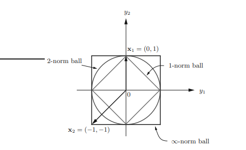
A polyhedron is just the intersection of some halfspaces and hyperplanes (see Figure 2.8). A polyhedron can be unbounded, while a bounded polyhedron is called a polytope, e.g., any 1-norm ball and $\infty$-norm ball of finite radius are polytopes.
Remark 2.3 It can be seen that the $\ell$-dimensional space $\mathbb{R}^{\ell}$ (also an affine set) cannot be expressed in the standard form (2.41) with either nonzero $\mathbf{A}$ or nonzero $\mathbf{C}$, and so it is not a polyhedron for any $\ell \in \mathbb{Z}{++}$. However, because any affine set in $\mathbb{R}^{\ell}$ can be expressed as (2.7) and each $\mathbf{x}$ in the set satisfies (2.8), this implies that the affine set must be a polyhedron if its affine dimension is strictly less than $\ell$. For instance, any subspaces with dimension less than $n$ in $\mathbb{R}^{n}$, and any hyperplane that is defined by a normal vector $\mathbf{a} \neq \mathbf{0}$ and a point $\mathbf{x}{0}$ on the hyperplane, i.e.,
$$
\mathcal{H}\left(\mathbf{a}, \mathbf{x}{0}\right)=\left{\mathbf{x} \mid \mathbf{a}^{T}\left(\mathbf{x}-\mathbf{x}{0}\right)=0\right}=\left{\mathbf{x}_{0}\right}+\mathcal{R}(\mathbf{a})^{\perp}
$$
in $\mathbb{R}^{n}$, and rays, line segments, and halfspaces are all polyhedra.
凸优化代写
数学代写|凸优化作业代写Convex Optimization代考|Hyperplanes and halfspaces
超平面是仿射集(因此是凸集)并且具有以下形式
H=\left{\mathbf{x} \mid \mathbf{a}^{T} \mathbf{x}=b\right} \subset \mathbb{R}^{n},H=\left{\mathbf{x} \mid \mathbf{a}^{T} \mathbf{x}=b\right} \subset \mathbb{R}^{n},
在哪里\mathbf{a} \in \mathbb{R}^{n} \反斜杠\left{\mathbf{0}_{n}\right}\mathbf{a} \in \mathbb{R}^{n} \反斜杠\left{\mathbf{0}_{n}\right}是超平面的法向量,并且b∈R. 解析地,它是一个线性方程组的解集X. 在几何意义上,超平面可以解释为具有恒定内积 (b) 与法向量 (a) 的点集。自从 affdim(H)=n−1,
超平面(2.30)也可以表示为
H=\operatorname{aff}\left{\mathbf{s}{1}, \ldots, \mathbf{s}{n}\right} \subset \mathbb{R}^{n},H=\operatorname{aff}\left{\mathbf{s}{1}, \ldots, \mathbf{s}{n}\right} \subset \mathbb{R}^{n},
在哪里\left{\mathbf{s}{1}, \ldots, \mathbf{s}{n}\right} \subset H\left{\mathbf{s}{1}, \ldots, \mathbf{s}{n}\right} \subset H是任何仿射独立集。然后可以看出
$$
\left{乙≜[s2−s1,…,sn−s1]∈Rn×(n−1) 和 暗淡(R(乙))=n−1 乙吨一种=0n−1, IE ,R(乙)⊥=R(一种)\对。$$ 暗示法线向量 a 可以从\left{\mathbf{s}{1}, \ldots, \mathbf{s}_{n}\right}\left{\mathbf{s}{1}, \ldots, \mathbf{s}_{n}\right}高达一个比例因子。
超平面H定义在(2.30)划分Rn分成两个封闭的半空间,如下所示:
\begin{aligned} &H_{-}=\left{\mathbf{x} \mid \mathbf{a}^{T} \mathbf{x} \leq b\right} \ &H_{+}=\left{\ mathbf{x} \mid \mathbf{a}^{T} \mathbf{x} \geq b\right} \end{对齐}\begin{aligned} &H_{-}=\left{\mathbf{x} \mid \mathbf{a}^{T} \mathbf{x} \leq b\right} \ &H_{+}=\left{\ mathbf{x} \mid \mathbf{a}^{T} \mathbf{x} \geq b\right} \end{对齐}
所以它们中的每一个都是一个(非平凡的)线性不等式的解集。注意一种=∇(一种吨X)表示线性函数的最大增加方向一种吨X. 以上两种说法H−和H+对于给定的一种≠0, 不是唯一的,而如果它们是唯一的一种被归一化,使得|一种|2=1. 而且,H−∩H+=H.
一个开放的半空间是一组形式
H_{–}=\left{\mathbf{x} \mid \mathbf{a}^{T} \mathbf{x}b\right}H_{–}=\left{\mathbf{x} \mid \mathbf{a}^{T} \mathbf{x}b\right}
在哪里一种∈Rn,一种≠0, 和b∈R.
数学代写|凸优化作业代写Convex Optimization代考|Euclidean balls and ellipsoids
一个欧几里得球(或简单地说,球)Rn具有以下形式:
B\left(\mathbf{x}{c}, r\right)=\left{\mathbf{x} \mid\left|\mathbf{x}-\mathbf{x}{c}\right|_{ 2} \leq r\right}=\left{\mathbf{x} \mid\left(\mathbf{x}-\mathbf{x}{c}\right)^{T}\left(\mathbf{x }-\mathbf{x}{c}\right) \leq r^{2}\right},B\left(\mathbf{x}{c}, r\right)=\left{\mathbf{x} \mid\left|\mathbf{x}-\mathbf{x}{c}\right|_{ 2} \leq r\right}=\left{\mathbf{x} \mid\left(\mathbf{x}-\mathbf{x}{c}\right)^{T}\left(\mathbf{x }-\mathbf{x}{c}\right) \leq r^{2}\right},
在哪里r>0. 向量XC是球的中心和正标量r是它的半径(见图 2.7)。欧几里得球也是一个2范数球,为了简单起见,没有明确提及相关范数的球在下文中指的是欧几里得球。欧几里得球的另一个常见表示是B\left(\mathbf{x}{c}, r\right)=\left{\mathbf{x}{c}+r \mathbf{u} \mid|\mathbf{u}|{2} \leq 1\右}B\left(\mathbf{x}{c}, r\right)=\left{\mathbf{x}{c}+r \mathbf{u} \mid|\mathbf{u}|{2} \leq 1\右}
可以很容易地证明欧几里得球是一个凸集。
凸性证明:让X1和X2∈乙(XC,r), IE,|X1−XC|2≤r和|X2− XC|2≤r. 然后,
|θX1+(1−θ)X2−XC|2=|θX1+(1−θ)X2−[θXC+(1−θ)XC]|2 =|θ(X1−XC)+(1−θ)(X2−XC)|2 ≤|θ(X1−XC)|2+|(1−θ)(X2−XC)|2 ≤θr+(1−θ)r =r, 对全部 0≤θ≤1
因此,θX1+(1−θ)X2∈乙(XC,r)对全部θ∈[0,1],因此我们证明了乙(XC,r)是凸的。
一个相关的凸集族是椭球体(见图2.7),其形式为
\mathcal{E}=\left{\mathbf{x} \mid\left(\mathbf{x}-\mathbf{x}{c}\right)^{T} \mathbf{P}^{-1} \left(\mathbf{x}-\mathbf{x}{c}\right) \leq 1\right},\mathcal{E}=\left{\mathbf{x} \mid\left(\mathbf{x}-\mathbf{x}{c}\right)^{T} \mathbf{P}^{-1} \left(\mathbf{x}-\mathbf{x}{c}\right) \leq 1\right},
在哪里磷∈小号++n和向量XC是椭球的中心。矩阵磷确定椭球从中心向各个方向延伸的距离;的半轴长度和由λ一世, 在哪里λ一世是的特征值磷. 请注意,球是椭球体磷=r2一世n在哪里r>0. 椭球的另一种常见表示是\mathcal{E}=\left{\mathbf{x}{c}+\mathbf{A u} \mid|\mathbf{u}|_{2} \leq 1\right}\mathcal{E}=\left{\mathbf{x}{c}+\mathbf{A u} \mid|\mathbf{u}|_{2} \leq 1\right}
在哪里一种是方阵且非奇异的。椭球体和由 (2.38) 表示的实际上是 2 范数球的图像B(\mathbf{0}, 1)=\left{\mathbf{u} \in \mathbb{R}^{n} \mid|\mathbf{u}|_{2} \leq 1\right}B(\mathbf{0}, 1)=\left{\mathbf{u} \in \mathbb{R}^{n} \mid|\mathbf{u}|_{2} \leq 1\right}通过一个
仿射映射XC+一种在(参见(2.58)), 在哪里一种=(磷1/2)吨, 下面将给出证明。对于椭球的表达式(2.38),奇异值一种,σ一世(一种)=λ一世(半轴长度)以比表达式 (2.37) 更直接的方式表征椭圆体的结构。
椭球表示(2.38)和凸性的证明:让
磷=问Λ问吨=(磷1/2)吨磷1/2
(和在D的磷≻0), 在哪里Λ=诊断(λ1,λ2,…,λn)和
磷1/2=Λ1/2问吨,
其中Λ1/2=诊断(λ1,λ2,…,λn). 然后
磷−1=问Λ−1问吨=磷−1/2(磷−1/2)吨,磷−1/2=问Λ−1/2
根据椭球的定义,我们有
\begin{对齐} \mathcal{E} &=\left{\mathbf{x} \mid\left(\mathbf{x}-\mathbf{x}{c}\right)^{T} \mathbf{P }^{-1}\left(\mathbf{x}-\mathbf{x}{c}\right) \leq 1\right} \ &=\left{\mathbf{x} \mid\left(\mathbf {x}-\mathbf{x}{c}\right)^{T} \mathbf{Q} \mathbf{\Lambda}^{-1} \mathbf{Q}^{T}\left(\mathbf{ x}-\mathbf{x}{c}\right) \leq 1\right} \end{对齐}\begin{对齐} \mathcal{E} &=\left{\mathbf{x} \mid\left(\mathbf{x}-\mathbf{x}{c}\right)^{T} \mathbf{P }^{-1}\left(\mathbf{x}-\mathbf{x}{c}\right) \leq 1\right} \ &=\left{\mathbf{x} \mid\left(\mathbf {x}-\mathbf{x}{c}\right)^{T} \mathbf{Q} \mathbf{\Lambda}^{-1} \mathbf{Q}^{T}\left(\mathbf{ x}-\mathbf{x}{c}\right) \leq 1\right} \end{对齐}
让和=X−XC. 然后\mathcal{E}=\left{\mathbf{x}{c}+\mathbf{z} \mid \mathbf{z}^{T} \mathbf{Q} \mathbf{\Lambda}^{-1} \mathbf{Q}^{T} \mathbf{z} \leq 1\right}\mathcal{E}=\left{\mathbf{x}{c}+\mathbf{z} \mid \mathbf{z}^{T} \mathbf{Q} \mathbf{\Lambda}^{-1} \mathbf{Q}^{T} \mathbf{z} \leq 1\right}
现在,通过让在=Λ−1/2问吨和=(磷−1/2)吨和,然后我们得到
\mathcal{E}=\left{\mathbf{x}{c}+\left(\mathbf{P}^{1 / 2}\right)^{T} \mathbf{u} \mid|\mathbf{ u}|{2} \leq 1\right}\mathcal{E}=\left{\mathbf{x}{c}+\left(\mathbf{P}^{1 / 2}\right)^{T} \mathbf{u} \mid|\mathbf{ u}|{2} \leq 1\right}
正好是 (2.38)(磷1/2)吨取而代之一种.
数学代写|凸优化作业代写Convex Optimization代考|Polyhedra
多面体是一个非空凸集,定义为有限数量的线性等式和不等式的解集:
\begin{aligned} \mathcal{P} &=\left{\mathbf{x} \mid \mathbf{a}{i}^{T} \mathbf{x} \leq b{i}, i=1, 2, \ldots, m, \mathbf{c}{j}^{T} \mathbf{x}=d{j}, j=1,2, \ldots, p\right} \ &=\left{\ mathbf{x} \mid \mathbf{A} \mathbf{x} \preceq \mathbf{b}=\left(b_{1}, \ldots, b_{m}\right), \mathbf{C x}= \mathbf{d}=\left(d_{1}, \ldots, d_{p}\right)\right} \end{对齐}\begin{aligned} \mathcal{P} &=\left{\mathbf{x} \mid \mathbf{a}{i}^{T} \mathbf{x} \leq b{i}, i=1, 2, \ldots, m, \mathbf{c}{j}^{T} \mathbf{x}=d{j}, j=1,2, \ldots, p\right} \ &=\left{\ mathbf{x} \mid \mathbf{A} \mathbf{x} \preceq \mathbf{b}=\left(b_{1}, \ldots, b_{m}\right), \mathbf{C x}= \mathbf{d}=\left(d_{1}, \ldots, d_{p}\right)\right} \end{对齐}
在哪里 ”⪯“代表分量不等式,一种∈R米×n和C∈Rp×n是行为 $\mathbf{a} {j}^{T} \mathrm{~s}的矩阵一种nd\mathbf{c} {j}^{T}\mathrm{~s},r和sp和C吨一世在和l是,一种nd\mathbf{A} \neq \mathbf{0}这r\mathbf{C} \neq \mathbf{0}米在s吨b和吨r在和.ñ这吨和吨H一种吨和一世吨H和rm=0这r只要其他参数是有限且非零的,就允许 p=0$。
多面体只是一些半空间和超平面的交集(见图 2.8)。多面体可以是无界的,而有界多面体称为多面体,例如,任何 1 范数球和∞有限半径的范数球是多面体。
备注 2.3 可以看出,ℓ维空间Rℓ(也是仿射集)不能用标准形式(2.41)表示,其中任一非零一种或非零C, 所以它不是任何一个多面体ℓ∈从++. 然而,因为任何仿射集在Rℓ可以表示为 (2.7) 并且每个X在集合满足 (2.8) 中,这意味着如果仿射集的仿射维数严格小于ℓ. 例如,任何维度小于n在Rn,以及由法线向量定义的任何超平面一种≠0和一点X0在超平面上,即
\mathcal{H}\left(\mathbf{a}, \mathbf{x}{0}\right)=\left{\mathbf{x} \mid \mathbf{a}^{T}\left(\mathbf {x}-\mathbf{x}{0}\right)=0\right}=\left{\mathbf{x}_{0}\right}+\mathcal{R}(\mathbf{a})^ {\perp}\mathcal{H}\left(\mathbf{a}, \mathbf{x}{0}\right)=\left{\mathbf{x} \mid \mathbf{a}^{T}\left(\mathbf {x}-\mathbf{x}{0}\right)=0\right}=\left{\mathbf{x}_{0}\right}+\mathcal{R}(\mathbf{a})^ {\perp}
在Rn,而射线、线段和半空间都是多面体。

统计代写请认准statistics-lab™. statistics-lab™为您的留学生涯保驾护航。
金融工程代写
金融工程是使用数学技术来解决金融问题。金融工程使用计算机科学、统计学、经济学和应用数学领域的工具和知识来解决当前的金融问题,以及设计新的和创新的金融产品。
非参数统计代写
非参数统计指的是一种统计方法,其中不假设数据来自于由少数参数决定的规定模型;这种模型的例子包括正态分布模型和线性回归模型。
广义线性模型代考
广义线性模型(GLM)归属统计学领域,是一种应用灵活的线性回归模型。该模型允许因变量的偏差分布有除了正态分布之外的其它分布。
术语 广义线性模型(GLM)通常是指给定连续和/或分类预测因素的连续响应变量的常规线性回归模型。它包括多元线性回归,以及方差分析和方差分析(仅含固定效应)。
有限元方法代写
有限元方法(FEM)是一种流行的方法,用于数值解决工程和数学建模中出现的微分方程。典型的问题领域包括结构分析、传热、流体流动、质量运输和电磁势等传统领域。
有限元是一种通用的数值方法,用于解决两个或三个空间变量的偏微分方程(即一些边界值问题)。为了解决一个问题,有限元将一个大系统细分为更小、更简单的部分,称为有限元。这是通过在空间维度上的特定空间离散化来实现的,它是通过构建对象的网格来实现的:用于求解的数值域,它有有限数量的点。边界值问题的有限元方法表述最终导致一个代数方程组。该方法在域上对未知函数进行逼近。[1] 然后将模拟这些有限元的简单方程组合成一个更大的方程系统,以模拟整个问题。然后,有限元通过变化微积分使相关的误差函数最小化来逼近一个解决方案。
tatistics-lab作为专业的留学生服务机构,多年来已为美国、英国、加拿大、澳洲等留学热门地的学生提供专业的学术服务,包括但不限于Essay代写,Assignment代写,Dissertation代写,Report代写,小组作业代写,Proposal代写,Paper代写,Presentation代写,计算机作业代写,论文修改和润色,网课代做,exam代考等等。写作范围涵盖高中,本科,研究生等海外留学全阶段,辐射金融,经济学,会计学,审计学,管理学等全球99%专业科目。写作团队既有专业英语母语作者,也有海外名校硕博留学生,每位写作老师都拥有过硬的语言能力,专业的学科背景和学术写作经验。我们承诺100%原创,100%专业,100%准时,100%满意。
随机分析代写
随机微积分是数学的一个分支,对随机过程进行操作。它允许为随机过程的积分定义一个关于随机过程的一致的积分理论。这个领域是由日本数学家伊藤清在第二次世界大战期间创建并开始的。
时间序列分析代写
随机过程,是依赖于参数的一组随机变量的全体,参数通常是时间。 随机变量是随机现象的数量表现,其时间序列是一组按照时间发生先后顺序进行排列的数据点序列。通常一组时间序列的时间间隔为一恒定值(如1秒,5分钟,12小时,7天,1年),因此时间序列可以作为离散时间数据进行分析处理。研究时间序列数据的意义在于现实中,往往需要研究某个事物其随时间发展变化的规律。这就需要通过研究该事物过去发展的历史记录,以得到其自身发展的规律。
回归分析代写
多元回归分析渐进(Multiple Regression Analysis Asymptotics)属于计量经济学领域,主要是一种数学上的统计分析方法,可以分析复杂情况下各影响因素的数学关系,在自然科学、社会和经济学等多个领域内应用广泛。
MATLAB代写
MATLAB 是一种用于技术计算的高性能语言。它将计算、可视化和编程集成在一个易于使用的环境中,其中问题和解决方案以熟悉的数学符号表示。典型用途包括:数学和计算算法开发建模、仿真和原型制作数据分析、探索和可视化科学和工程图形应用程序开发,包括图形用户界面构建MATLAB 是一个交互式系统,其基本数据元素是一个不需要维度的数组。这使您可以解决许多技术计算问题,尤其是那些具有矩阵和向量公式的问题,而只需用 C 或 Fortran 等标量非交互式语言编写程序所需的时间的一小部分。MATLAB 名称代表矩阵实验室。MATLAB 最初的编写目的是提供对由 LINPACK 和 EISPACK 项目开发的矩阵软件的轻松访问,这两个项目共同代表了矩阵计算软件的最新技术。MATLAB 经过多年的发展,得到了许多用户的投入。在大学环境中,它是数学、工程和科学入门和高级课程的标准教学工具。在工业领域,MATLAB 是高效研究、开发和分析的首选工具。MATLAB 具有一系列称为工具箱的特定于应用程序的解决方案。对于大多数 MATLAB 用户来说非常重要,工具箱允许您学习和应用专业技术。工具箱是 MATLAB 函数(M 文件)的综合集合,可扩展 MATLAB 环境以解决特定类别的问题。可用工具箱的领域包括信号处理、控制系统、神经网络、模糊逻辑、小波、仿真等。