数学代写|有限元方法代写Finite Element Method代考|Find 2022
如果你也在 怎样代写有限元方法Finite Element Method这个学科遇到相关的难题,请随时右上角联系我们的24/7代写客服。
有限元法是一种系统的方法,将无限维函数空间中的函数首先转换为有限维函数空间中的函数,最后转换为用数值方法可以处理的普通向量。
statistics-lab™ 为您的留学生涯保驾护航 在代写有限元方法Finite Element Method方面已经树立了自己的口碑, 保证靠谱, 高质且原创的统计Statistics代写服务。我们的专家在代写有限元方法Finite Element Method代写方面经验极为丰富,各种代写有限元方法Finite Element Method相关的作业也就用不着说。
我们提供的有限元方法Finite Element Method及其相关学科的代写,服务范围广, 其中包括但不限于:
- Statistical Inference 统计推断
- Statistical Computing 统计计算
- Advanced Probability Theory 高等概率论
- Advanced Mathematical Statistics 高等数理统计学
- (Generalized) Linear Models 广义线性模型
- Statistical Machine Learning 统计机器学习
- Longitudinal Data Analysis 纵向数据分析
- Foundations of Data Science 数据科学基础
数学代写|有限元方法代写Finite Element Method代考|General overview
The physical processes encountered in all branches of sciences and engineering can be classified into two major categories: time-dependent processes and stationary processes. Time-dependent processes describe evolutions in which quantities of interest change with time. If the quantities of interest cease to change in an evolution then the evolution is said to have reached a stationary state. Not all evolutions have stationary states. The evolutions without a stationary state are often referred to as unsteady processes. Stationary processes are those in which the quantities of interest do not depend upon time. For a stationary process to be valid or viable, it must correspond to the stationary state of an evolution. Every process in nature is an evolution. Nonetheless it is sometimes convenient to consider their stationary state. In this book we only consider non-stationary processes, i.e. evolutions that may have a stationary state or may be unsteady.
A mathematical description of most stationary processes in sciences and engineering often leads to a system of ordinary or partial differential equations. These mathematical descriptions of the stationary processes are referred to as boundary value problems (BVPs). Since stationary processes are independent of time, the partial differential equations describing their behavior only involve dependent variables and space coordinates as independent variables. On the other hand, mathematical descriptions of evolutions lead to partial differential equations in dependent variables, space coordinates, and time and are referred to as initial value problems (IVPs).
In case of simple physical systems, the mathematical descriptions of IVPs may be simple enough to permit analytical solutions. However, most physical systems of interest may be quite complicated and their mathematical description (IVPs) may be complex enough not to permit analytical solutions. In such cases, two alternatives are possible. In the first case, one could undertake simplifications of the mathematical descriptions to a point that analytical solutions are possible. In this approach, the simplified forms may not be descriptive of the actual behavior and sometimes this simplification may not be possible at all. In the second alternative, we abandon the possibility of theoretical solutions altogether as viable means of solving complex practical problems involving IVPs and instead we resort to numerical meth-ods for obtaining numerical solutions of IVPs. The finite element method (FEM) is one such method of solving IVPs numerically and constitutes the subject matter of this book. Before we delve deeper into the FEM for IVPs, it is perhaps fitting to discuss a little about the broader classes of available methods for obtaining numerical solutions of IVPs.
数学代写|有限元方法代写Finite Element Method代考|Space-time coupled methods of approximation
We note that since $\phi=\phi(x, t)$, the solution exhibits simultaneous dependence on spatial coordinates $x$ and time $t$. This feature is intrinsic in the mathematical description (1.1) of the physics.
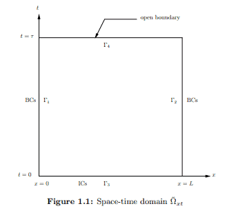
Thus, the most rational approach to undertake for the solution of (1.1) (approximate or otherwise) is to preserve simultaneous dependence of $\phi$ on $x$ and $t$. Such methods are known as space-time coupled methods. Broadly speaking, in such methods time $t$ is treated as another independent variable in addition to spatial coordinates. Fig. $1.1$ shows space-time domain $\bar{\Omega}{x t}=$ $\Omega{x t} \cup \Gamma ; \Gamma=\cup_{i=1}^{4} \Gamma_{i}$ with closed boundary $\Gamma$. For the sake of discussion, as an example we could have a boundary condition $(\mathrm{BC})$ at $x=0 \forall t \in[0, \tau]$, boundary $\Gamma_{1}$, as well as at $x=L \forall t \in[0, \tau]$, boundary $\Gamma_{2}$, and an initial condition $(\mathrm{IC})$ at $t=0 \forall x \in[0, L]$, boundary $\Gamma_{3}$. Boundary $\Gamma_{4}$ at final value of time $t=\tau$ is open, i.e. at this boundary only the evolution (the solution of (1.1) subjected to these $\mathrm{BCs}$ and $\mathrm{IC})$, will yield the function $\phi(x, \tau)$ and its spatial and time derivatives.
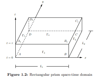
When the initial value problem contains two spatial coordinates, we have space-time slab $\bar{\Omega}{x t}$ shown in Fig. $1.2$ in which $$ \Omega{x t}=\left(0, L_{1}\right) \times\left(0, L_{2}\right) \times(0, \tau)
$$
is a prism. In this case $\Gamma_{1}, \Gamma_{2}, \Gamma_{3}$, and $\Gamma_{4}$ are faces of the prism (surfaces). For illustration, the possible choices of BCs and ICs could be: BCs on $\Gamma_{1}=$ $A D D_{1} A_{1}$ and $\Gamma_{2}=B C C_{1} B_{1}$, IC on $\Gamma_{3}=A B C D$, and $\Gamma_{4}=A_{1} B_{1} C_{1} D_{1}$ is the open boundary. This concept of space-time slab can be extended for three spatial dimensions and time. Using space-time domain shown in Fig. $1.1$ or $1.2$ and treating time as another independent variable, we could consider the following methods of approximation.
有限元方法代考
数学代写|有限元方法代写Finite Element Method代考|General overview
在科学和工程的所有分支中遇到的物理过程可以分为两大类:时间相关过程和平稳过程。时间相关过程描述了兴趣数量随时间变化的演变。如果感兴趣的数量在演化中停止变化,则称演化已达到静止状态。并非所有演化都有静止状态。没有稳态的演化通常被称为非稳态过程。平稳过程是那些感兴趣的数量不依赖于时间的过程。为了使平稳过程有效或可行,它必须对应于演化的平稳状态。自然界中的每一个过程都是一种进化。尽管如此,有时考虑它们的静止状态是很方便的。
对科学和工程中大多数平稳过程的数学描述通常会导致一个常微分方程或偏微分方程系统。这些平稳过程的数学描述被称为边界值问题(BVP)。由于平稳过程与时间无关,因此描述其行为的偏微分方程仅涉及因变量和空间坐标作为自变量。另一方面,演化的数学描述导致因变量、空间坐标和时间的偏微分方程,被称为初始值问题 (IVP)。
在简单物理系统的情况下,IVP 的数学描述可能足够简单以允许解析解。然而,大多数感兴趣的物理系统可能非常复杂,并且它们的数学描述 (IVP) 可能复杂到不允许解析解。在这种情况下,有两种选择是可能的。在第一种情况下,人们可以对数学描述进行简化,使解析解成为可能。在这种方法中,简化形式可能无法描述实际行为,有时这种简化可能根本不可能。在第二种选择中,我们完全放弃了将理论解作为解决涉及 IVP 的复杂实际问题的可行方法的可能性,而是采用数值方法来获得 IVP 的数值解。有限元法 (FEM) 就是这样一种数值求解 IVP 的方法,它构成了本书的主题。在我们深入研究 IVP 的 FEM 之前,可能适合讨论一下获得 IVP 数值解的更广泛的可用方法类别。
数学代写|有限元方法代写Finite Element Method代考|Space-time coupled methods of approximation
我们注意到,由于 $\phi=\phi(x, t)$, 该解决方案表现出同时依赖于空间坐标 $x$ 和时间 $t$. 这个特征在物理学的数学描述 (1.1) 中是固有的。
因此,解决 (1.1) 的最合理的方法 (近似或其他) 是保持同时依赖 $\phi$ 上 $x$ 和 $t$. 这种方法被称为时空耦合方法。从广 义上讲,在这种方法中,时间 $t$ 被视为除空间坐标之外的另一个自变量。如图。1.1显示时空域 $\bar{\Omega} x t=$ $\Omega x t \cup \Gamma ; \Gamma=\cup_{i=1}^{4} \Gamma_{i}$ 有封闭边界 $\Gamma$. 为了讨论,作为一个例子,我们可以有一个边界条件 $(\mathrm{BC})$ 在
$x=0 \forall t \in[0, \tau]$ ,边界 $\Gamma_{1}$ ,以及在 $x=L \forall t \in[0, \tau]$, 边界 $\Gamma_{2}$ ,和一个初始条件 (IC)在 $t=0 \forall x \in[0, L]$ ,边 界 $\Gamma_{3}$. 边界 $\Gamma_{4}$ 在最终时间值 $t=\tau$ 是开放的,即在这个边界上只有演化 ( (1.1) 的解受到这些BCs和IC),将产 生函数 $\phi(x, \tau)$ 及其空间和时间导数。
当初值问题包含两个空间坐标时,我们有时空平板 $\bar{\Omega} x t$ 如图所示。 $1.2$ 其中
$$
\Omega x t=\left(0, L_{1}\right) \times\left(0, L_{2}\right) \times(0, \tau)
$$
是棱镜。在这种情况下 $\Gamma_{1}, \Gamma_{2}, \Gamma_{3}$ ,和 $\Gamma_{4}$ 是棱镜的面 (表面)。举例来说,BCs 和 ICs 的可能选择可能是: BCs on $\Gamma_{1}=A D D_{1} A_{1}$ 和 $\Gamma_{2}=B C C_{1} B_{1}$ ,图标 $\Gamma_{3}=A B C D$ ,和 $\Gamma_{4}=A_{1} B_{1} C_{1} D_{1}$ 是开放边界。这种时空 平板的概念可以扩展到三个空间维度和时间。使用如图所示的时空域。1.1或者 $1.2$ 并将时间视为另一个自变量, 我们可以考虑以下近似方法。

统计代写请认准statistics-lab™. statistics-lab™为您的留学生涯保驾护航。
金融工程代写
金融工程是使用数学技术来解决金融问题。金融工程使用计算机科学、统计学、经济学和应用数学领域的工具和知识来解决当前的金融问题,以及设计新的和创新的金融产品。
非参数统计代写
非参数统计指的是一种统计方法,其中不假设数据来自于由少数参数决定的规定模型;这种模型的例子包括正态分布模型和线性回归模型。
广义线性模型代考
广义线性模型(GLM)归属统计学领域,是一种应用灵活的线性回归模型。该模型允许因变量的偏差分布有除了正态分布之外的其它分布。
术语 广义线性模型(GLM)通常是指给定连续和/或分类预测因素的连续响应变量的常规线性回归模型。它包括多元线性回归,以及方差分析和方差分析(仅含固定效应)。
有限元方法代写
有限元方法(FEM)是一种流行的方法,用于数值解决工程和数学建模中出现的微分方程。典型的问题领域包括结构分析、传热、流体流动、质量运输和电磁势等传统领域。
有限元是一种通用的数值方法,用于解决两个或三个空间变量的偏微分方程(即一些边界值问题)。为了解决一个问题,有限元将一个大系统细分为更小、更简单的部分,称为有限元。这是通过在空间维度上的特定空间离散化来实现的,它是通过构建对象的网格来实现的:用于求解的数值域,它有有限数量的点。边界值问题的有限元方法表述最终导致一个代数方程组。该方法在域上对未知函数进行逼近。[1] 然后将模拟这些有限元的简单方程组合成一个更大的方程系统,以模拟整个问题。然后,有限元通过变化微积分使相关的误差函数最小化来逼近一个解决方案。
tatistics-lab作为专业的留学生服务机构,多年来已为美国、英国、加拿大、澳洲等留学热门地的学生提供专业的学术服务,包括但不限于Essay代写,Assignment代写,Dissertation代写,Report代写,小组作业代写,Proposal代写,Paper代写,Presentation代写,计算机作业代写,论文修改和润色,网课代做,exam代考等等。写作范围涵盖高中,本科,研究生等海外留学全阶段,辐射金融,经济学,会计学,审计学,管理学等全球99%专业科目。写作团队既有专业英语母语作者,也有海外名校硕博留学生,每位写作老师都拥有过硬的语言能力,专业的学科背景和学术写作经验。我们承诺100%原创,100%专业,100%准时,100%满意。
随机分析代写
随机微积分是数学的一个分支,对随机过程进行操作。它允许为随机过程的积分定义一个关于随机过程的一致的积分理论。这个领域是由日本数学家伊藤清在第二次世界大战期间创建并开始的。
时间序列分析代写
随机过程,是依赖于参数的一组随机变量的全体,参数通常是时间。 随机变量是随机现象的数量表现,其时间序列是一组按照时间发生先后顺序进行排列的数据点序列。通常一组时间序列的时间间隔为一恒定值(如1秒,5分钟,12小时,7天,1年),因此时间序列可以作为离散时间数据进行分析处理。研究时间序列数据的意义在于现实中,往往需要研究某个事物其随时间发展变化的规律。这就需要通过研究该事物过去发展的历史记录,以得到其自身发展的规律。
回归分析代写
多元回归分析渐进(Multiple Regression Analysis Asymptotics)属于计量经济学领域,主要是一种数学上的统计分析方法,可以分析复杂情况下各影响因素的数学关系,在自然科学、社会和经济学等多个领域内应用广泛。
MATLAB代写
MATLAB 是一种用于技术计算的高性能语言。它将计算、可视化和编程集成在一个易于使用的环境中,其中问题和解决方案以熟悉的数学符号表示。典型用途包括:数学和计算算法开发建模、仿真和原型制作数据分析、探索和可视化科学和工程图形应用程序开发,包括图形用户界面构建MATLAB 是一个交互式系统,其基本数据元素是一个不需要维度的数组。这使您可以解决许多技术计算问题,尤其是那些具有矩阵和向量公式的问题,而只需用 C 或 Fortran 等标量非交互式语言编写程序所需的时间的一小部分。MATLAB 名称代表矩阵实验室。MATLAB 最初的编写目的是提供对由 LINPACK 和 EISPACK 项目开发的矩阵软件的轻松访问,这两个项目共同代表了矩阵计算软件的最新技术。MATLAB 经过多年的发展,得到了许多用户的投入。在大学环境中,它是数学、工程和科学入门和高级课程的标准教学工具。在工业领域,MATLAB 是高效研究、开发和分析的首选工具。MATLAB 具有一系列称为工具箱的特定于应用程序的解决方案。对于大多数 MATLAB 用户来说非常重要,工具箱允许您学习和应用专业技术。工具箱是 MATLAB 函数(M 文件)的综合集合,可扩展 MATLAB 环境以解决特定类别的问题。可用工具箱的领域包括信号处理、控制系统、神经网络、模糊逻辑、小波、仿真等。