如果你也在 怎样代写有限元方法Finite Element Method这个学科遇到相关的难题，请随时右上角联系我们的24/7代写客服。

有限元法是一种系统的方法，将无限维函数空间中的函数首先转换为有限维函数空间中的函数，最后转换为用数值方法可以处理的普通向量。

statistics-lab™ 为您的留学生涯保驾护航 在代写有限元方法Finite Element Method方面已经树立了自己的口碑, 保证靠谱, 高质且原创的统计Statistics代写服务。我们的专家在代写有限元方法Finite Element Method代写方面经验极为丰富，各种代写有限元方法Finite Element Method相关的作业也就用不着说。

我们提供的有限元方法Finite Element Method及其相关学科的代写，服务范围广, 其中包括但不限于:

• Statistical Inference 统计推断
• Statistical Computing 统计计算
• Advanced Probability Theory 高等概率论
• Advanced Mathematical Statistics 高等数理统计学
• (Generalized) Linear Models 广义线性模型
• Statistical Machine Learning 统计机器学习
• Longitudinal Data Analysis 纵向数据分析
• Foundations of Data Science 数据科学基础

数学代写|有限元方法代写Finite Element Method代考|Boundary value problem

In this chapter, we consider the solution of the Sturm-Liouville type second order differential equation,
$$
\frac{d}{d x}\left(a \frac{d u}{d x}\right)+p u+q=0 \text { in } 0<x<L
$$
where $a(x), p(x)$ and $q(x)$ are specified functions and $u(x)$ is the dependent variable. The admissible boundary conditions for this problem are as follows: at $x=0$ : either $u$ is specified or $-\frac{d u}{d x}=\alpha_0 u+\beta_0$ at $x=L$ : either $u$ is specified or $\frac{d u}{d x}=\alpha_0 u+\beta_0$
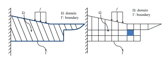
where $\alpha_{-}$and $\beta_{-}$are known coefficients on the boundaries. See Section 2.4.5.1 on the signs. The domain, $0<x<L$, is shown in Fig. 4.1. In what follows, the weighted residual method is implemented segment-by-segment over the solution domain.

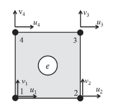
Spatial segmentation of the solution domain is known as discretization. In a one-dimensional problem discretization is straightforward as demonstrated in Fig. 4.1. The domain is divided into $N_E$ interconnected segments, known as elements. Each element has two ends (boundaries) through which the elements are connected. Thus, there are a total of $N_E+1$ boundary connectivity points known as boundary-nodes. As it will become clear in Section 4.3, there are also elements with internal nodes that are used to improve the order of polynomial interpolation along the element.

In a one dimensional domain, the element-to-node connectivity relationship is straightforward as shown below. This is especially true if the elements only have two nodes and the nodes are numbered consecutively starting from number one.

Element connectivity: Consider a discretization where elements are numbered consecutively as $1 \leq i \leq N_E$. It is easy to see that element- $i$ will be connected to nodes $i$ and $i+1$.
Element- $i$ will span the range $x_i<x<x_{i+1}$, and its length will be, $L^{(i)}=x_{i+1}-x_i$
The element-to-node connectivity of the higher order elements, i.e. those with internal nodes, can be handled in a similar manner.

While the weighted residual method can be developed in the (global) coordinate system $(x)$ of the boundary value problem, it is simpler to use an element coordinate system $\left(x^{\prime}\right)$ placed on the lower numbered node of the element (Fig. 4.1). In what follows the finite element form of the weak form of the boundary value problem will be developed over the element subdomain.

数学代写|有限元方法代写Finite Element Method代考|Heat transfer in a one-dimensional domain

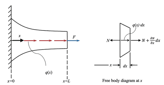
Conduction in a $1 \mathrm{D}$ medium that spans the length $x^{\prime}=0$ to $L^{(e)}$ is governed by Eq. (2.171),
$$
A Q+\frac{d}{d x^{\prime}}\left(k A \frac{d T}{d x^{\prime}}\right)=0 \text { in } 0<x^{\prime}<L^{(e)}
$$
where $Q$ is the rate of heat generation per unit volume, $k$ is the conductivity and $A$ is the cross sectional area. In case the heat is transferred from a thin fin to a surrounding fluid at temperature $T_{\infty}$ the energy balance can be approximated as follows:
$$
A Q+\frac{d}{d x^{\prime}}\left(k A \frac{d T}{d x^{\prime}}\right)+h P\left(T_{\infty}-T\right)=0 \text { in } 0<x^{\prime}<L^{(e)}
$$
where $P$ is the perimeter of the fin, $h$ is the convection coefficient. Heat flux is considered to be specified on the boundaries,
$$
\left(-k \frac{d T}{d x^{\prime}}\right)0 n=f{B 1} \text { and }\left(-k \frac{d T}{d x^{\prime}}\right){L^{(c)}} n=f{B 2}
$$
Note that $n$ represents the unit normal of the boundary with $n=-1$ and 1 at $x=0$ and $L$, respectively.
Insulated Boundary $: f_{B i}=f_B(t)$
Convected Boundary : $f_{B i}=h\left(T-T_{\infty}\right)$
Radiated Boundary : $f_{B i}=\sigma \psi\left(T^4-T_s^4\right)=\left[\sigma \psi\left(T^3-T_S^3\right)\right]\left(T-T_S\right)$
where $i=1,2$. Note that $f_{B i}$ for convection and radiation given in (2.4.18) are considered positive.

有限元方法代考

数学代写|有限元方法代写Finite Element Method代考|Boundary value problem

在本章中，我们考虑 Sturm-Liouville 型二阶微分方程的解，
$$
\frac{d}{d x}\left(a \frac{d u}{d x}\right)+p u+q=0 \text { in } 0<x<L
$$
在哪里 $a(x), p(x)$ 和 $q(x)$ 是指定的功能和 $u(x)$ 是因变量。该问题的可接受边界条件如下： $x=0$ ：任何 一个 $u$ 指定或 $-\frac{d u}{d x}=\alpha_0 u+\beta_0$ 在 $x=L:$ 任何一个 $u$ 指定或 $\frac{d u}{d x}=\alpha_0 u+\beta_0$
在哪里 $\alpha_{-}$和 $\beta_{-}$是边界上的已知系数。请参阅第 2.4.5.1 节中的标志。域名， $0<x<L$, 如图 4.1 所 示。接下来，加权残差法在解域上逐段实现。
解域的空间分割称为离散化。在一维问题中，离散化很简单，如图 $4.1$ 所示。域分为 $N_E$ 相互连接的部 分，称为元素。每个元素都有两个端点 (边界)，元素通过这两个端点连接。因此，总共有 $N_E+1$ 边界 连接点称为边界节点。正如在第 $4.3$ 节中将变得清楚的那样，还有一些带有内部节点的元素用于改进沿元 素的多项式揷值的阶数。
在一维域中，元素到节点的连接关系很简单，如下所示。如果元素只有两个节点并且节点从第一个开始连 续编号，则尤其如此。
元素连通性：考虑离散化，其中元素连续编号为 $1 \leq i \leq N_E$. 很容易看出该元素 $-i$ 将连接到节点 $i$ 和 $i+1$.
元素- $i$ 将跨越范围 $x_i<x<x_{i+1}$ ，其长度为 $L^{(i)}=x_{i+1}-x_i$
高阶元素的元素到节点的连接性，即那些具有内部节点的元素，可以用类似的方式处理。
而加权残差法可以在 (全局) 坐标系下开发 $(x)$ 边界值问题，使用元素坐标系更简单 $\left(x^{\prime}\right)$ 放置在元素的较 低编号节点上（图 4.1）。接下来将在单元子域上展开边值问题的弱形式的有限元形式。

数学代写|有限元方法代写Finite Element Method代考|Heat transfer in a one-dimensional domain

在一个传导 $1 \mathrm{D}$ 跨越长度的介质 $x^{\prime}=0$ 到 $L^{(e)}$ 受方程式约束。(2.171)，
$$
A Q+\frac{d}{d x^{\prime}}\left(k A \frac{d T}{d x^{\prime}}\right)=0 \text { in } 0<x^{\prime}<L^{(e)}
$$
在哪里 $Q$ 是每单位体积的热生成率， $k$ 是电导率和 $A$ 是横截面积。如果热量从薄翅片传递到周围温度较高 的流体 $T_{\infty}$ 能量平衡可以近似如下:
$$
A Q+\frac{d}{d x^{\prime}}\left(k A \frac{d T}{d x^{\prime}}\right)+h P\left(T_{\infty}-T\right)=0 \text { in } 0<x^{\prime}<L^{(e)}
$$
在哪里 $P$ 是鳍的周长， $h$ 是对流系数。热通量被认为是在边界上指定的，
$$
\left(-k \frac{d T}{d x^{\prime}}\right) 0 n=f B 1 \text { and }\left(-k \frac{d T}{d x^{\prime}}\right) L^{(c)} n=f B 2
$$
注意 $n$ 表示边界的单位法线 $n=-1$ 和 1 在 $x=0$ 和 $L$ ，分别。
绝缘边界: $f_{B i}=f_B(t)$
对流边界： $f_{B i}=h\left(T-T_{\infty}\right)$
辐射边界: $f_{B i}=\sigma \psi\left(T^4-T_s^4\right)=\left[\sigma \psi\left(T^3-T_S^3\right)\right]\left(T-T_S\right)$
在哪里 $i=1,2$. 注意 $f_{B i}$ (2.4.18) 中给出的对流和辐射被认为是正的。

统计代写请认准statistics-lab™. statistics-lab™为您的留学生涯保驾护航。

金融工程代写

金融工程是使用数学技术来解决金融问题。金融工程使用计算机科学、统计学、经济学和应用数学领域的工具和知识来解决当前的金融问题，以及设计新的和创新的金融产品。

非参数统计代写

非参数统计指的是一种统计方法，其中不假设数据来自于由少数参数决定的规定模型；这种模型的例子包括正态分布模型和线性回归模型。

广义线性模型代考

广义线性模型（GLM）归属统计学领域，是一种应用灵活的线性回归模型。该模型允许因变量的偏差分布有除了正态分布之外的其它分布。

术语 广义线性模型（GLM）通常是指给定连续和/或分类预测因素的连续响应变量的常规线性回归模型。它包括多元线性回归，以及方差分析和方差分析（仅含固定效应）。

有限元方法代写

有限元方法（FEM）是一种流行的方法，用于数值解决工程和数学建模中出现的微分方程。典型的问题领域包括结构分析、传热、流体流动、质量运输和电磁势等传统领域。

有限元是一种通用的数值方法，用于解决两个或三个空间变量的偏微分方程（即一些边界值问题）。为了解决一个问题，有限元将一个大系统细分为更小、更简单的部分，称为有限元。这是通过在空间维度上的特定空间离散化来实现的，它是通过构建对象的网格来实现的：用于求解的数值域，它有有限数量的点。边界值问题的有限元方法表述最终导致一个代数方程组。该方法在域上对未知函数进行逼近。[1] 然后将模拟这些有限元的简单方程组合成一个更大的方程系统，以模拟整个问题。然后，有限元通过变化微积分使相关的误差函数最小化来逼近一个解决方案。

tatistics-lab作为专业的留学生服务机构，多年来已为美国、英国、加拿大、澳洲等留学热门地的学生提供专业的学术服务，包括但不限于Essay代写，Assignment代写，Dissertation代写，Report代写，小组作业代写，Proposal代写，Paper代写，Presentation代写，计算机作业代写，论文修改和润色，网课代做，exam代考等等。写作范围涵盖高中，本科，研究生等海外留学全阶段，辐射金融，经济学，会计学，审计学，管理学等全球99%专业科目。写作团队既有专业英语母语作者，也有海外名校硕博留学生，每位写作老师都拥有过硬的语言能力，专业的学科背景和学术写作经验。我们承诺100%原创，100%专业，100%准时，100%满意。

随机分析代写

随机微积分是数学的一个分支，对随机过程进行操作。它允许为随机过程的积分定义一个关于随机过程的一致的积分理论。这个领域是由日本数学家伊藤清在第二次世界大战期间创建并开始的。

时间序列分析代写

随机过程，是依赖于参数的一组随机变量的全体，参数通常是时间。 随机变量是随机现象的数量表现，其时间序列是一组按照时间发生先后顺序进行排列的数据点序列。通常一组时间序列的时间间隔为一恒定值（如1秒，5分钟，12小时，7天，1年），因此时间序列可以作为离散时间数据进行分析处理。研究时间序列数据的意义在于现实中，往往需要研究某个事物其随时间发展变化的规律。这就需要通过研究该事物过去发展的历史记录，以得到其自身发展的规律。

回归分析代写

多元回归分析渐进（Multiple Regression Analysis Asymptotics）属于计量经济学领域，主要是一种数学上的统计分析方法，可以分析复杂情况下各影响因素的数学关系，在自然科学、社会和经济学等多个领域内应用广泛。

MATLAB代写

MATLAB 是一种用于技术计算的高性能语言。它将计算、可视化和编程集成在一个易于使用的环境中，其中问题和解决方案以熟悉的数学符号表示。典型用途包括：数学和计算算法开发建模、仿真和原型制作数据分析、探索和可视化科学和工程图形应用程序开发，包括图形用户界面构建MATLAB 是一个交互式系统，其基本数据元素是一个不需要维度的数组。这使您可以解决许多技术计算问题，尤其是那些具有矩阵和向量公式的问题，而只需用 C 或 Fortran 等标量非交互式语言编写程序所需的时间的一小部分。MATLAB 名称代表矩阵实验室。MATLAB 最初的编写目的是提供对由 LINPACK 和 EISPACK 项目开发的矩阵软件的轻松访问，这两个项目共同代表了矩阵计算软件的最新技术。MATLAB 经过多年的发展，得到了许多用户的投入。在大学环境中，它是数学、工程和科学入门和高级课程的标准教学工具。在工业领域，MATLAB 是高效研究、开发和分析的首选工具。MATLAB 具有一系列称为工具箱的特定于应用程序的解决方案。对于大多数 MATLAB 用户来说非常重要，工具箱允许您学习和应用专业技术。工具箱是 MATLAB 函数（M 文件）的综合集合，可扩展 MATLAB 环境以解决特定类别的问题。可用工具箱的领域包括信号处理、控制系统、神经网络、模糊逻辑、小波、仿真等。

R语言代写	问卷设计与分析代写
PYTHON代写	回归分析与线性模型代写
MATLAB代写	方差分析与试验设计代写
STATA代写	机器学习/统计学习代写
SPSS代写	计量经济学代写
EVIEWS代写	时间序列分析代写
EXCEL代写	深度学习代写
SQL代写	各种数据建模与可视化代写

如果你也在 怎样代写有限元方法Finite Element Method这个学科遇到相关的难题，请随时右上角联系我们的24/7代写客服。

有限元法是一种系统的方法，将无限维函数空间中的函数首先转换为有限维函数空间中的函数，最后转换为用数值方法可以处理的普通向量。

statistics-lab™ 为您的留学生涯保驾护航 在代写有限元方法Finite Element Method方面已经树立了自己的口碑, 保证靠谱, 高质且原创的统计Statistics代写服务。我们的专家在代写有限元方法Finite Element Method代写方面经验极为丰富，各种代写有限元方法Finite Element Method相关的作业也就用不着说。

我们提供的有限元方法Finite Element Method及其相关学科的代写，服务范围广, 其中包括但不限于:

• Statistical Inference 统计推断
• Statistical Computing 统计计算
• Advanced Probability Theory 高等概率论
• Advanced Mathematical Statistics 高等数理统计学
• (Generalized) Linear Models 广义线性模型
• Statistical Machine Learning 统计机器学习
• Longitudinal Data Analysis 纵向数据分析
• Foundations of Data Science 数据科学基础

数学代写|有限元方法代写Finite Element Method代考|Equation of motion of a beam

We will next develop the equations of motion for a beam subjected to external loading. First these equations will be developed in terms of the internal bending moment $M$ and shear force resultant $V$. In this form, these equations apply to both EB and Timoshenko beam theories. Let’s consider the deflection of a beam subjected to distributed force $q_y(x, t)$. Free body diagram of an infinitesimally small segment of a beam subjected to $q_y$ is shown in Fig. 2.19. The balance of forces acting in the transverse direction should be equal to the acceleration of the beam segment. This is expressed as follows:
$$
\begin{aligned}
V-\left(V+\frac{\partial V}{\partial x} d x\right)-q_y d x &=\rho A d x \frac{\partial^2 v}{\partial t^2} \
q_y+\frac{\partial V}{\partial x} &=\rho A \frac{\partial^2 v}{\partial t^2}
\end{aligned}
$$

The balance of moments acting on the small beam segment, about the $z$-axis gives,
$$
\begin{aligned}
&\rho I \frac{\partial^2 \alpha}{\partial t^2}=-M+\left(M+\frac{\partial M}{\partial x} d x\right)-V d x+q_y \frac{d x^2}{2} \
&\rho I \frac{\partial^2 \alpha}{\partial t^2}=\frac{\partial M}{\partial x}-V+q_y \frac{d x}{2}
\end{aligned}
$$
where $I$ is the second moment of area of the beam. Taking the limit as $d x \rightarrow 0$ we find
$$
\frac{\partial M}{\partial x}=V+\rho I \frac{\partial^2 \alpha}{\partial t^2}
$$
Thus we see that equation of motion of the beam is represented by two coupled Eqs. (2.133) and (2.136), where $M, V, v$ and $\alpha$ are the unknown variables. The kinematics of deformation allow further simplifications.

数学代写|有限元方法代写Finite Element Method代考|Stresses in an Euler–Bernoulli beam

Using Hooke’s law, the longitudinal stress due to bending can be derived as follows:
$$
\sigma_x=-E\left(y \frac{d^2 v}{d x^2}\right)
$$
This is also known as the bending stress. Eq. (2.139) shows that the bending stress is zero on the neutral axis $(y=0)$ and otherwise varies linearly through the thickness of the beam (Fig. 2.19). Close inspection of this figure shows that the bending stress can be represented by a resultant bending moment about the neutral axis. This gives rise to the moment-curvature relationship as follows:
$$
\begin{aligned}
&M=\int_{-h / 2}^{h / 2} \sigma_x y b d y=-E \frac{d^2 v}{d x^2} \int_{-h / 2}^{h / 2} y^2 b d y \
&M=-E I \frac{d^2 v}{d x^2}
\end{aligned}
$$
where the second moment of area of the cross-section of the beam is defined as follows:
$$
I=\int_{-h / 2}^{h / 2} y^2 b d y
$$
Note that for small beam deflections the curvature of the deflected beam is approximately given by the term, $d^2 v / d x^2$. By combining Eqs. (2.139) and (2.140a), a relationship between the bending moment and the bending stress can be obtained as follows:
$$
\sigma_x=-\frac{M y}{I}
$$
In case the beam deflection is due to the combined action of transverse loads and external bending moments, then internal shear force will develop in the beam. It is shown a bit later in this document that the shear force resultant is given by the following relationship:
$$
V=\frac{d M}{d x}=-\frac{d}{d x}\left(E I \frac{d^2 v}{d x^2}\right)
$$
The stress-displacement relationships for the Euler-Bernoulli beam are summarized in Table 2.1.

有限元方法代考

数学代写|有限元方法代写有限元法代考|梁的运动方程

我们接下来将推导受外力作用的梁的运动方程。首先，这些方程将根据内弯矩$M$和剪力合成$V$来发展。在这种形式下，这些方程适用于EB和Timoshenko束理论。让我们考虑受分布力$q_y(x, t)$作用的梁的挠度。图2.19显示了受$q_y$作用的梁的无穷小段的自由体图。作用于横方向的力的平衡应等于梁段的加速度。表达式如下:
$$
\begin{aligned}
V-\left(V+\frac{\partial V}{\partial x} d x\right)-q_y d x &=\rho A d x \frac{\partial^2 v}{\partial t^2} \
q_y+\frac{\partial V}{\partial x} &=\rho A \frac{\partial^2 v}{\partial t^2}
\end{aligned}
$$

作用在小梁段上的力矩平衡，约$z$ -轴给出，
$$
\begin{aligned}
&\rho I \frac{\partial^2 \alpha}{\partial t^2}=-M+\left(M+\frac{\partial M}{\partial x} d x\right)-V d x+q_y \frac{d x^2}{2} \
&\rho I \frac{\partial^2 \alpha}{\partial t^2}=\frac{\partial M}{\partial x}-V+q_y \frac{d x}{2}
\end{aligned}
$$
，其中$I$是梁面积的第二个弯矩。取极限$d x \rightarrow 0$，得到
$$
\frac{\partial M}{\partial x}=V+\rho I \frac{\partial^2 \alpha}{\partial t^2}
$$
，由此可知，梁的运动方程由两个耦合的方程式表示。(2.133)和(2.136)，其中$M, V, v$和$\alpha$为未知变量。变形的运动学可以进一步简化

数学代写|有限元方法代写有限元法代考|欧拉-伯努利梁中的应力

根据胡克定律，弯曲引起的纵向应力可以推导为:
$$
\sigma_x=-E\left(y \frac{d^2 v}{d x^2}\right)
$$
这也被称为弯曲应力。式(2.139)表明，弯曲应力在中性轴$(y=0)$上为零，否则随梁的厚度线性变化(图2.19)。仔细观察这个图可以看出弯曲应力可以用绕中性轴的合成弯矩表示。这就产生了如下的弯矩-曲率关系:
$$
\begin{aligned}
&M=\int_{-h / 2}^{h / 2} \sigma_x y b d y=-E \frac{d^2 v}{d x^2} \int_{-h / 2}^{h / 2} y^2 b d y \
&M=-E I \frac{d^2 v}{d x^2}
\end{aligned}
$$
其中梁横截面面积的第二个弯矩定义如下:
$$
I=\int_{-h / 2}^{h / 2} y^2 b d y
$$
注意，对于较小的梁挠度，挠度梁的曲率近似由术语$d^2 v / d x^2$给出。通过合并方程式。(2.139)和(2.140a)，弯矩与弯曲应力的关系为:
$$
\sigma_x=-\frac{M y}{I}
$$
如果梁的挠度是由于横向荷载和外弯矩的共同作用，则梁内部会产生剪力。在本文档后面稍作说明，剪力合成由以下关系给出:
$$
V=\frac{d M}{d x}=-\frac{d}{d x}\left(E I \frac{d^2 v}{d x^2}\right)
$$
欧拉-伯努利梁的应力-位移关系在表2.1中总结

统计代写请认准statistics-lab™. statistics-lab™为您的留学生涯保驾护航。

金融工程代写

金融工程是使用数学技术来解决金融问题。金融工程使用计算机科学、统计学、经济学和应用数学领域的工具和知识来解决当前的金融问题，以及设计新的和创新的金融产品。

非参数统计代写

非参数统计指的是一种统计方法，其中不假设数据来自于由少数参数决定的规定模型；这种模型的例子包括正态分布模型和线性回归模型。

广义线性模型代考

广义线性模型（GLM）归属统计学领域，是一种应用灵活的线性回归模型。该模型允许因变量的偏差分布有除了正态分布之外的其它分布。

术语 广义线性模型（GLM）通常是指给定连续和/或分类预测因素的连续响应变量的常规线性回归模型。它包括多元线性回归，以及方差分析和方差分析（仅含固定效应）。

有限元方法代写

有限元方法（FEM）是一种流行的方法，用于数值解决工程和数学建模中出现的微分方程。典型的问题领域包括结构分析、传热、流体流动、质量运输和电磁势等传统领域。

有限元是一种通用的数值方法，用于解决两个或三个空间变量的偏微分方程（即一些边界值问题）。为了解决一个问题，有限元将一个大系统细分为更小、更简单的部分，称为有限元。这是通过在空间维度上的特定空间离散化来实现的，它是通过构建对象的网格来实现的：用于求解的数值域，它有有限数量的点。边界值问题的有限元方法表述最终导致一个代数方程组。该方法在域上对未知函数进行逼近。[1] 然后将模拟这些有限元的简单方程组合成一个更大的方程系统，以模拟整个问题。然后，有限元通过变化微积分使相关的误差函数最小化来逼近一个解决方案。

tatistics-lab作为专业的留学生服务机构，多年来已为美国、英国、加拿大、澳洲等留学热门地的学生提供专业的学术服务，包括但不限于Essay代写，Assignment代写，Dissertation代写，Report代写，小组作业代写，Proposal代写，Paper代写，Presentation代写，计算机作业代写，论文修改和润色，网课代做，exam代考等等。写作范围涵盖高中，本科，研究生等海外留学全阶段，辐射金融，经济学，会计学，审计学，管理学等全球99%专业科目。写作团队既有专业英语母语作者，也有海外名校硕博留学生，每位写作老师都拥有过硬的语言能力，专业的学科背景和学术写作经验。我们承诺100%原创，100%专业，100%准时，100%满意。

随机分析代写

随机微积分是数学的一个分支，对随机过程进行操作。它允许为随机过程的积分定义一个关于随机过程的一致的积分理论。这个领域是由日本数学家伊藤清在第二次世界大战期间创建并开始的。

时间序列分析代写

随机过程，是依赖于参数的一组随机变量的全体，参数通常是时间。 随机变量是随机现象的数量表现，其时间序列是一组按照时间发生先后顺序进行排列的数据点序列。通常一组时间序列的时间间隔为一恒定值（如1秒，5分钟，12小时，7天，1年），因此时间序列可以作为离散时间数据进行分析处理。研究时间序列数据的意义在于现实中，往往需要研究某个事物其随时间发展变化的规律。这就需要通过研究该事物过去发展的历史记录，以得到其自身发展的规律。

回归分析代写

多元回归分析渐进（Multiple Regression Analysis Asymptotics）属于计量经济学领域，主要是一种数学上的统计分析方法，可以分析复杂情况下各影响因素的数学关系，在自然科学、社会和经济学等多个领域内应用广泛。

MATLAB代写

MATLAB 是一种用于技术计算的高性能语言。它将计算、可视化和编程集成在一个易于使用的环境中，其中问题和解决方案以熟悉的数学符号表示。典型用途包括：数学和计算算法开发建模、仿真和原型制作数据分析、探索和可视化科学和工程图形应用程序开发，包括图形用户界面构建MATLAB 是一个交互式系统，其基本数据元素是一个不需要维度的数组。这使您可以解决许多技术计算问题，尤其是那些具有矩阵和向量公式的问题，而只需用 C 或 Fortran 等标量非交互式语言编写程序所需的时间的一小部分。MATLAB 名称代表矩阵实验室。MATLAB 最初的编写目的是提供对由 LINPACK 和 EISPACK 项目开发的矩阵软件的轻松访问，这两个项目共同代表了矩阵计算软件的最新技术。MATLAB 经过多年的发展，得到了许多用户的投入。在大学环境中，它是数学、工程和科学入门和高级课程的标准教学工具。在工业领域，MATLAB 是高效研究、开发和分析的首选工具。MATLAB 具有一系列称为工具箱的特定于应用程序的解决方案。对于大多数 MATLAB 用户来说非常重要，工具箱允许您学习和应用专业技术。工具箱是 MATLAB 函数（M 文件）的综合集合，可扩展 MATLAB 环境以解决特定类别的问题。可用工具箱的领域包括信号处理、控制系统、神经网络、模糊逻辑、小波、仿真等。

R语言代写	问卷设计与分析代写
PYTHON代写	回归分析与线性模型代写
MATLAB代写	方差分析与试验设计代写
STATA代写	机器学习/统计学习代写
SPSS代写	计量经济学代写
EVIEWS代写	时间序列分析代写
EXCEL代写	深度学习代写
SQL代写	各种数据建模与可视化代写

如果你也在 怎样代写有限元方法Finite Element Method这个学科遇到相关的难题，请随时右上角联系我们的24/7代写客服。

有限元法是一种系统的方法，将无限维函数空间中的函数首先转换为有限维函数空间中的函数，最后转换为用数值方法可以处理的普通向量。

statistics-lab™ 为您的留学生涯保驾护航 在代写有限元方法Finite Element Method方面已经树立了自己的口碑, 保证靠谱, 高质且原创的统计Statistics代写服务。我们的专家在代写有限元方法Finite Element Method代写方面经验极为丰富，各种代写有限元方法Finite Element Method相关的作业也就用不着说。

我们提供的有限元方法Finite Element Method及其相关学科的代写，服务范围广, 其中包括但不限于:

• Statistical Inference 统计推断
• Statistical Computing 统计计算
• Advanced Probability Theory 高等概率论
• Advanced Mathematical Statistics 高等数理统计学
• (Generalized) Linear Models 广义线性模型
• Statistical Machine Learning 统计机器学习
• Longitudinal Data Analysis 纵向数据分析
• Foundations of Data Science 数据科学基础

数学代写|有限元方法代写Finite Element Method代考|Potential possessed by applied loads

In general, the external forces that act on a given deformable volume can be classified as body forces and surface forces. In vector notation these are expressed as follows:

$$
\begin{array}{lll}
\text { Body force } & \left{F_B\right}=\left{\begin{array}{lll}
F_{B x} & F_{B y} & F_{B z}
\end{array}\right}^T \
\text { Surface traction } & {T}=\left{\begin{array}{lll}
q_x & q_y & q_z
\end{array}\right}^T \
\text { Concentrated force } & {F} &
\end{array}
$$
The deformation vector $\vec{u}$ is expressed by using the vector representation as follows:
$$
{u}=\left{\begin{array}{lll}
u_x & u_y & u_z
\end{array}\right}^T
$$
In general, the work required to move a force $\vec{F}$ through a displacement $\vec{u}$ is expressed as follows:
$$
W=\vec{F} \cdot \vec{u} \text { or } W={u}^T{F}
$$
Considering that the body force acts per unit volume of the material, and the surface traction acts over the outer surface $S(=\Gamma)$ of the body, the total work done by the external forces is given as follows:
$$
W=\int_V{u}^T\left{F_b\right} d V+\int_S{u}^T{T} d S+\sum\left{u_F\right}^T{F}
$$
where $\left{u_F\right}$ represents the deflections where the concentrated loads ${F}$ are applied. The potential due this work is $\Omega=-W$ as before.

数学代写|有限元方法代写Finite Element Method代考|Mechanics of a flexible beam

Mechanics of a deformable medium that describe the three-dimensional loading and deformation states are described in the previous sections. If the plane stress and plane strain conditions can be satisfied by the geometry and the loading conditions, the analysis can be reduced to two spatial dimensions. Beam theory is another form of simplification that typically applies to long and slender deformable members that are typically loaded normal to their longitudinal axes $[1,5]$. For such structural members the analysis can be simplified to one spatial dimension.

A long $(L)$ and slender $(h \times b)$ beam subjected to a transverse distributed load $q_y$, transverse concentrated force $F$ and a bending moment $M_L$ is shown in Fig. 2.16. Such structural members resist external loads by developing internal bending moments $M(x)$ and transverse shear forces $V(x)$. The transverse deflection of the beam is $u_y$ and the longitudinal deflection is $u_x$. However, the customary notation for beam theory is $u=u_x$ and $v=u_y$, as depicted in Fig. 2.17. Both of these variables are functions of the longitudinal position $x$. If the external loading depends on time, then the beam deflection will also vary in time, $t$.

The following assumptions are made in order to develop the beam theory:
(1) transverse deflection $v$ is smaller than thickness $h$ of the beam $(v<h)$; (2) material is isotropic and behaves linearly and elastically; and (3) transverse normal stress $\sigma_y$ is negligible. The nature of the transverse shear strain gives rise to the two theories, as described below.

有限元方法代考

数学代写|有限元方法代写有限元法代考|施加载荷所具有的电位

.

一般来说，作用在给定变形体积上的外力可分为体力和表面力。用向量表示法表示如下:

$$
\begin{array}{lll}
\text { Body force } & \left{F_B\right}=\left{\begin{array}{lll}
F_{B x} & F_{B y} & F_{B z}
\end{array}\right}^T \
\text { Surface traction } & {T}=\left{\begin{array}{lll}
q_x & q_y & q_z
\end{array}\right}^T \
\text { Concentrated force } & {F} &
\end{array}
$$
变形向量 $\vec{u}$ 用向量表示如下:
$$
{u}=\left{\begin{array}{lll}
u_x & u_y & u_z
\end{array}\right}^T
$$一般来说，移动一个力所需做的功 $\vec{F}$ 通过位移 $\vec{u}$ 表达式为:
$$
W=\vec{F} \cdot \vec{u} \text { or } W={u}^T{F}
$$考虑到体力作用于材料的单位体积，表面牵引力作用于外表面 $S(=\Gamma)$ 对于物体，外力所做的总功为:
$$
W=\int_V{u}^T\left{F_b\right} d V+\int_S{u}^T{T} d S+\sum\left{u_F\right}^T{F}
$$
where $\left{u_F\right}$ 表示集中荷载处的挠度 ${F}$ 应用。这项工作的潜力是 $\Omega=-W$

数学代写|有限元方法代写有限元法代考|柔性梁的力学

描述三维加载和变形状态的可变形介质的力学在前面的章节中有描述。如果几何和加载条件都能满足平面应力和平面应变条件，则分析可简化为两个空间维度。梁理论是另一种简化形式，通常适用于长而细长的可变形构件，这些构件通常被垂直于其纵轴加载$[1,5]$。对于这种结构构件，分析可以简化到一个空间维度

图2.16所示为受横向分布荷载$q_y$、横向集中力$F$和弯矩$M_L$作用的长梁$(L)$和细长梁$(h \times b)$。这种结构构件通过发展内部弯矩$M(x)$和横向剪力$V(x)$来抵抗外部荷载。梁的横向挠度为$u_y$，纵向挠度为$u_x$。然而，束理论的习惯符号是$u=u_x$和$v=u_y$，如图2.17所示。这两个变量都是纵向位置$x$的函数。如果外部荷载取决于时间，那么梁的挠度也会随时间变化$t$ .

(1)横向挠度$v$小于梁的厚度$h$$(v<h)$;(2)材料是各向同性的，具有线性和弹性;(3)横向法向应力$\sigma_y$可以忽略不计。横向剪切应变的性质产生了这两种理论，如下所述

统计代写请认准statistics-lab™. statistics-lab™为您的留学生涯保驾护航。

金融工程代写

金融工程是使用数学技术来解决金融问题。金融工程使用计算机科学、统计学、经济学和应用数学领域的工具和知识来解决当前的金融问题，以及设计新的和创新的金融产品。

非参数统计代写

非参数统计指的是一种统计方法，其中不假设数据来自于由少数参数决定的规定模型；这种模型的例子包括正态分布模型和线性回归模型。

广义线性模型代考

广义线性模型（GLM）归属统计学领域，是一种应用灵活的线性回归模型。该模型允许因变量的偏差分布有除了正态分布之外的其它分布。

术语 广义线性模型（GLM）通常是指给定连续和/或分类预测因素的连续响应变量的常规线性回归模型。它包括多元线性回归，以及方差分析和方差分析（仅含固定效应）。

有限元方法代写

有限元方法（FEM）是一种流行的方法，用于数值解决工程和数学建模中出现的微分方程。典型的问题领域包括结构分析、传热、流体流动、质量运输和电磁势等传统领域。

有限元是一种通用的数值方法，用于解决两个或三个空间变量的偏微分方程（即一些边界值问题）。为了解决一个问题，有限元将一个大系统细分为更小、更简单的部分，称为有限元。这是通过在空间维度上的特定空间离散化来实现的，它是通过构建对象的网格来实现的：用于求解的数值域，它有有限数量的点。边界值问题的有限元方法表述最终导致一个代数方程组。该方法在域上对未知函数进行逼近。[1] 然后将模拟这些有限元的简单方程组合成一个更大的方程系统，以模拟整个问题。然后，有限元通过变化微积分使相关的误差函数最小化来逼近一个解决方案。

tatistics-lab作为专业的留学生服务机构，多年来已为美国、英国、加拿大、澳洲等留学热门地的学生提供专业的学术服务，包括但不限于Essay代写，Assignment代写，Dissertation代写，Report代写，小组作业代写，Proposal代写，Paper代写，Presentation代写，计算机作业代写，论文修改和润色，网课代做，exam代考等等。写作范围涵盖高中，本科，研究生等海外留学全阶段，辐射金融，经济学，会计学，审计学，管理学等全球99%专业科目。写作团队既有专业英语母语作者，也有海外名校硕博留学生，每位写作老师都拥有过硬的语言能力，专业的学科背景和学术写作经验。我们承诺100%原创，100%专业，100%准时，100%满意。

随机分析代写

随机微积分是数学的一个分支，对随机过程进行操作。它允许为随机过程的积分定义一个关于随机过程的一致的积分理论。这个领域是由日本数学家伊藤清在第二次世界大战期间创建并开始的。

时间序列分析代写

随机过程，是依赖于参数的一组随机变量的全体，参数通常是时间。 随机变量是随机现象的数量表现，其时间序列是一组按照时间发生先后顺序进行排列的数据点序列。通常一组时间序列的时间间隔为一恒定值（如1秒，5分钟，12小时，7天，1年），因此时间序列可以作为离散时间数据进行分析处理。研究时间序列数据的意义在于现实中，往往需要研究某个事物其随时间发展变化的规律。这就需要通过研究该事物过去发展的历史记录，以得到其自身发展的规律。

回归分析代写

多元回归分析渐进（Multiple Regression Analysis Asymptotics）属于计量经济学领域，主要是一种数学上的统计分析方法，可以分析复杂情况下各影响因素的数学关系，在自然科学、社会和经济学等多个领域内应用广泛。

MATLAB代写

MATLAB 是一种用于技术计算的高性能语言。它将计算、可视化和编程集成在一个易于使用的环境中，其中问题和解决方案以熟悉的数学符号表示。典型用途包括：数学和计算算法开发建模、仿真和原型制作数据分析、探索和可视化科学和工程图形应用程序开发，包括图形用户界面构建MATLAB 是一个交互式系统，其基本数据元素是一个不需要维度的数组。这使您可以解决许多技术计算问题，尤其是那些具有矩阵和向量公式的问题，而只需用 C 或 Fortran 等标量非交互式语言编写程序所需的时间的一小部分。MATLAB 名称代表矩阵实验室。MATLAB 最初的编写目的是提供对由 LINPACK 和 EISPACK 项目开发的矩阵软件的轻松访问，这两个项目共同代表了矩阵计算软件的最新技术。MATLAB 经过多年的发展，得到了许多用户的投入。在大学环境中，它是数学、工程和科学入门和高级课程的标准教学工具。在工业领域，MATLAB 是高效研究、开发和分析的首选工具。MATLAB 具有一系列称为工具箱的特定于应用程序的解决方案。对于大多数 MATLAB 用户来说非常重要，工具箱允许您学习和应用专业技术。工具箱是 MATLAB 函数（M 文件）的综合集合，可扩展 MATLAB 环境以解决特定类别的问题。可用工具箱的领域包括信号处理、控制系统、神经网络、模糊逻辑、小波、仿真等。

R语言代写	问卷设计与分析代写
PYTHON代写	回归分析与线性模型代写
MATLAB代写	方差分析与试验设计代写
STATA代写	机器学习/统计学习代写
SPSS代写	计量经济学代写
EVIEWS代写	时间序列分析代写
EXCEL代写	深度学习代写
SQL代写	各种数据建模与可视化代写

如果你也在 怎样代写有限元方法Finite Element Method这个学科遇到相关的难题，请随时右上角联系我们的24/7代写客服。

有限元法是一种系统的方法，将无限维函数空间中的函数首先转换为有限维函数空间中的函数，最后转换为用数值方法可以处理的普通向量。

statistics-lab™ 为您的留学生涯保驾护航 在代写有限元方法Finite Element Method方面已经树立了自己的口碑, 保证靠谱, 高质且原创的统计Statistics代写服务。我们的专家在代写有限元方法Finite Element Method代写方面经验极为丰富，各种代写有限元方法Finite Element Method相关的作业也就用不着说。

我们提供的有限元方法Finite Element Method及其相关学科的代写，服务范围广, 其中包括但不限于:

• Statistical Inference 统计推断
• Statistical Computing 统计计算
• Advanced Probability Theory 高等概率论
• Advanced Mathematical Statistics 高等数理统计学
• (Generalized) Linear Models 广义线性模型
• Statistical Machine Learning 统计机器学习
• Longitudinal Data Analysis 纵向数据分析
• Foundations of Data Science 数据科学基础

数学代写|有限元方法代写Finite Element Method代考|Total potential energy of conservative systems

A system is conservative if the work done by internal and external forces are both independent of the path taken between initial and final states. Here we consider conservative systems. Under this assumption, the total potential energy $\pi_p$ of a deformable body subjected to external forces is given by the following relationship,
$$
\pi_p=U+\Omega
$$
where $U$ is the strain energy of elastic distortion and $\Omega$ is the potential possessed by applied loads (by virtue of having the capacity to do work if displaced through a distance).
2.2.9.1 Total potential energy of a linear spring
In order to motivate the concept of strain energy let’s recall the familiar linear spring subjected to an axial load. The force-displacement relationship (Fig. 2.13) for a linear spring is given by the familiar relationship,
$$
F=k u
$$

where $k$ is the spring constant, and $u$ is the end displacement of spring.
Let us assume that for an external force of magnitude $F^$ the string stretches by an amount $u^$ Energy stored in the spring in the stretched configuration is found by computing the area under the force-displacement curve, and for a linear spring it is given as follows:
$$
\mathcal{U}=\frac{1}{2} k u^{* 2}
$$
The factor $1 / 2$ takes into account that the force $F$ increases linearly and slowly during deformation.

The work $W$ done by the force to stretch the spring by this amount is $W=F^* u^$. By doing this work, the load loses the same amount in potential. The potential of the applied load is expressed as follows: $$ \Omega=-W=-F^ u^*
$$
Note that here we assume that the load is regarded as acting at its full value, $F^$. The total potential energy of the system then becomes, $$ \pi_p=\frac{1}{2} k u^{ 2}-F^* u^*
$$

数学代写|有限元方法代写Finite Element Method代考|Total potential energy of an elastic body

We will next consider a deformable continuum, and the energy stored in it when it is loaded by external forces. In an elastic material, work done by internal forces is equal in magnitude to the change in strain energy.
Strain energy for one-dimensional deformation Let’s consider a bar under uniaxial tension (Fig. 2.14A). This bar is in a state of pure tensile stress. If we take an infinitesimally small volume from this bar as shown in Fig. 2.14B, we will see that it experiences a constant stress $\sigma$ and constant strain $\varepsilon$, along the $x$-axis.

The internal force in this state can be found as follows $d F=\sigma(d y d z)$ and the corresponding displacement from the relationship $\varepsilon=\Delta(d x) / d x$ as $d(d x)=\varepsilon d x$. If the material behaves in a linear elastic manner we can assume that the internal work is given by the familiar relationship:
$$
\frac{1}{2} d F d(d x)=\frac{1}{2} \sigma \varepsilon(d x d y d z)=\frac{1}{2} \sigma \varepsilon d V
$$
where $d V=(d x d y d z)$ represents the small volume of the element. Shortly, we will drop the assumption of linear elastic material, and generalize this relationship. For now, let’s state that the incremental internal work is stored in the material as incremental strain energyd $\mathcal{U}$,
$$
d \mathcal{U}=\frac{1}{2} \sigma \varepsilon d V
$$

The ratio of the strain energy to the volume of the material is the strain energy density $u$,
$$
u=\frac{d \mathcal{U}}{d V}=\frac{1}{2} \sigma \varepsilon
$$
Let’s next consider a material with nonlinear stress-strain relationship as shown in the Fig. 2.15. The increment of strain energy density $d u$ for a constant stress can be approximated as the area under the stress-strain curve for the strain increment $d \varepsilon$. This is depicted in Fig. $2.15$ and computed as follows:
$$
d u=\sigma d \varepsilon
$$

有限元方法代考

数学代写|有限元方法代写有限元法代考|保守系统的总势能

如果内力和外力所做的功与初始态和最终态之间的路径无关，则系统是保守的。这里我们考虑保守系统。在这种假设下，可变形体在外力作用下的总势能$\pi_p$由以下关系式给出，
$$
\pi_p=U+\Omega
$$
其中$U$是弹性变形的应变能，$\Omega$是施加的载荷所具有的势能(由于位移一段距离后具有功的能力)受轴向载荷的线性弹簧。线性弹簧的力-位移关系(图2.13)由熟悉的关系给出，
$$
F=k u
$$

其中$k$为弹簧常数，$u$为弹簧末端位移。让我们假设，对于一个大小为$F^$的外力，弦的拉伸量为$u^$在拉伸结构中，弹簧中储存的能量是通过计算力-位移曲线下的面积来找到的，对于一个线性弹簧，它被给出如下:
$$
\mathcal{U}=\frac{1}{2} k u^{* 2}
$$
因子$1 / 2$考虑到力$F$在变形过程中线性而缓慢地增加 将弹簧拉伸这个量的力做的功$W$是$W=F^* u^$。通过做这个功，负载损失了同样数量的电势。应用负载的潜力表示如下:$$ \Omega=-W=-F^ u^*
$$
注意，这里我们假设负载被视为在其全部值$F^$发挥作用。系统的总势能就变成$$ \pi_p=\frac{1}{2} k u^{ 2}-F^* u^*
$$

数学代写|有限元方法代写有限元法代考|弹性体总势能

我们接下来将考虑一个可变形的连续体，以及当它受外力加载时储存在它里面的能量。在弹性材料中，内力所作的功的大小等于应变能的变化。让我们考虑受单轴拉力的杆(图2.14A)。这根杆处于纯拉应力状态。如果我们取如图2.14B所示的这个杆的无穷小体积，我们会看到它沿着$x$ -轴经历恒定应力$\sigma$和恒定应变$\varepsilon$。

这种状态下的内力可以找到如下$d F=\sigma(d y d z)$，对应的位移从关系$\varepsilon=\Delta(d x) / d x$为$d(d x)=\varepsilon d x$。如果材料表现为线弹性的方式，我们可以假设内部功由熟悉的关系给出:
$$
\frac{1}{2} d F d(d x)=\frac{1}{2} \sigma \varepsilon(d x d y d z)=\frac{1}{2} \sigma \varepsilon d V
$$
，其中$d V=(d x d y d z)$表示元素的小体积。简而言之，我们将放弃线弹性材料的假设，并将这一关系推广。现在，让我们声明增量内部功存储在材料作为增量应变energyd $\mathcal{U}$，
$$
d \mathcal{U}=\frac{1}{2} \sigma \varepsilon d V
$$

应变能与材料体积的比值为应变能密度$u$，
$$
u=\frac{d \mathcal{U}}{d V}=\frac{1}{2} \sigma \varepsilon
$$
接下来让我们考虑如图2.15所示的具有非线性应力-应变关系的材料。恒定应力下应变能密度增量$d u$可近似为应变增量$d \varepsilon$的应力应变曲线下面积。这在图$2.15$中描述，并计算如下:
$$
d u=\sigma d \varepsilon
$$

统计代写请认准statistics-lab™. statistics-lab™为您的留学生涯保驾护航。

金融工程代写

金融工程是使用数学技术来解决金融问题。金融工程使用计算机科学、统计学、经济学和应用数学领域的工具和知识来解决当前的金融问题，以及设计新的和创新的金融产品。

非参数统计代写

非参数统计指的是一种统计方法，其中不假设数据来自于由少数参数决定的规定模型；这种模型的例子包括正态分布模型和线性回归模型。

广义线性模型代考

广义线性模型（GLM）归属统计学领域，是一种应用灵活的线性回归模型。该模型允许因变量的偏差分布有除了正态分布之外的其它分布。

术语 广义线性模型（GLM）通常是指给定连续和/或分类预测因素的连续响应变量的常规线性回归模型。它包括多元线性回归，以及方差分析和方差分析（仅含固定效应）。

有限元方法代写

有限元方法（FEM）是一种流行的方法，用于数值解决工程和数学建模中出现的微分方程。典型的问题领域包括结构分析、传热、流体流动、质量运输和电磁势等传统领域。

有限元是一种通用的数值方法，用于解决两个或三个空间变量的偏微分方程（即一些边界值问题）。为了解决一个问题，有限元将一个大系统细分为更小、更简单的部分，称为有限元。这是通过在空间维度上的特定空间离散化来实现的，它是通过构建对象的网格来实现的：用于求解的数值域，它有有限数量的点。边界值问题的有限元方法表述最终导致一个代数方程组。该方法在域上对未知函数进行逼近。[1] 然后将模拟这些有限元的简单方程组合成一个更大的方程系统，以模拟整个问题。然后，有限元通过变化微积分使相关的误差函数最小化来逼近一个解决方案。

tatistics-lab作为专业的留学生服务机构，多年来已为美国、英国、加拿大、澳洲等留学热门地的学生提供专业的学术服务，包括但不限于Essay代写，Assignment代写，Dissertation代写，Report代写，小组作业代写，Proposal代写，Paper代写，Presentation代写，计算机作业代写，论文修改和润色，网课代做，exam代考等等。写作范围涵盖高中，本科，研究生等海外留学全阶段，辐射金融，经济学，会计学，审计学，管理学等全球99%专业科目。写作团队既有专业英语母语作者，也有海外名校硕博留学生，每位写作老师都拥有过硬的语言能力，专业的学科背景和学术写作经验。我们承诺100%原创，100%专业，100%准时，100%满意。

随机分析代写

随机微积分是数学的一个分支，对随机过程进行操作。它允许为随机过程的积分定义一个关于随机过程的一致的积分理论。这个领域是由日本数学家伊藤清在第二次世界大战期间创建并开始的。

时间序列分析代写

随机过程，是依赖于参数的一组随机变量的全体，参数通常是时间。 随机变量是随机现象的数量表现，其时间序列是一组按照时间发生先后顺序进行排列的数据点序列。通常一组时间序列的时间间隔为一恒定值（如1秒，5分钟，12小时，7天，1年），因此时间序列可以作为离散时间数据进行分析处理。研究时间序列数据的意义在于现实中，往往需要研究某个事物其随时间发展变化的规律。这就需要通过研究该事物过去发展的历史记录，以得到其自身发展的规律。

回归分析代写

多元回归分析渐进（Multiple Regression Analysis Asymptotics）属于计量经济学领域，主要是一种数学上的统计分析方法，可以分析复杂情况下各影响因素的数学关系，在自然科学、社会和经济学等多个领域内应用广泛。

MATLAB代写

MATLAB 是一种用于技术计算的高性能语言。它将计算、可视化和编程集成在一个易于使用的环境中，其中问题和解决方案以熟悉的数学符号表示。典型用途包括：数学和计算算法开发建模、仿真和原型制作数据分析、探索和可视化科学和工程图形应用程序开发，包括图形用户界面构建MATLAB 是一个交互式系统，其基本数据元素是一个不需要维度的数组。这使您可以解决许多技术计算问题，尤其是那些具有矩阵和向量公式的问题，而只需用 C 或 Fortran 等标量非交互式语言编写程序所需的时间的一小部分。MATLAB 名称代表矩阵实验室。MATLAB 最初的编写目的是提供对由 LINPACK 和 EISPACK 项目开发的矩阵软件的轻松访问，这两个项目共同代表了矩阵计算软件的最新技术。MATLAB 经过多年的发展，得到了许多用户的投入。在大学环境中，它是数学、工程和科学入门和高级课程的标准教学工具。在工业领域，MATLAB 是高效研究、开发和分析的首选工具。MATLAB 具有一系列称为工具箱的特定于应用程序的解决方案。对于大多数 MATLAB 用户来说非常重要，工具箱允许您学习和应用专业技术。工具箱是 MATLAB 函数（M 文件）的综合集合，可扩展 MATLAB 环境以解决特定类别的问题。可用工具箱的领域包括信号处理、控制系统、神经网络、模糊逻辑、小波、仿真等。

R语言代写	问卷设计与分析代写
PYTHON代写	回归分析与线性模型代写
MATLAB代写	方差分析与试验设计代写
STATA代写	机器学习/统计学习代写
SPSS代写	计量经济学代写
EVIEWS代写	时间序列分析代写
EXCEL代写	深度学习代写
SQL代写	各种数据建模与可视化代写

如果你也在 怎样代写有限元方法Finite Element Method这个学科遇到相关的难题，请随时右上角联系我们的24/7代写客服。

有限元法是一种系统的方法，将无限维函数空间中的函数首先转换为有限维函数空间中的函数，最后转换为用数值方法可以处理的普通向量。

statistics-lab™ 为您的留学生涯保驾护航 在代写有限元方法Finite Element Method方面已经树立了自己的口碑, 保证靠谱, 高质且原创的统计Statistics代写服务。我们的专家在代写有限元方法Finite Element Method代写方面经验极为丰富，各种代写有限元方法Finite Element Method相关的作业也就用不着说。

我们提供的有限元方法Finite Element Method及其相关学科的代写，服务范围广, 其中包括但不限于:

• Statistical Inference 统计推断
• Statistical Computing 统计计算
• Advanced Probability Theory 高等概率论
• Advanced Mathematical Statistics 高等数理统计学
• (Generalized) Linear Models 广义线性模型
• Statistical Machine Learning 统计机器学习
• Longitudinal Data Analysis 纵向数据分析
• Foundations of Data Science 数据科学基础

数学代写|有限元方法代写Finite Element Method代考|Principal stresses and directions

Infinitely many planes can pass through a given point in a continuum, such as the plane that gives rise to the tetrahedron shown in Fig. 2.3. The normal and shear traction components $\sigma_{n n}$ and $\sigma_{n t}$ will vary according to the orientation of the cutting-plane. It is reasonable to assume that among these planes, there is one on which the shear tractions vanish, i.e., $\sigma_{n t}=0$. This plane is called the principal plane, and its orientation is called the principal orientation $\vec{n}{p}$. The normal component of the traction $\sigma{n n}$ acting on the principle plane has the magnitude $\lambda$ and it is named the principal stress.

The traction acting on the principal plane can be expressed by a simple vector argument and by using Eq. (2.17a) as follows:
$$
\begin{aligned}
&\vec{T}{n{p}}=\lambda \vec{n}{p} \ &\vec{T}{n_{p}}=[\sigma]^{T}\left{n_{p}\right}
\end{aligned}
$$
By combining these two relationships, we find,
$$
\begin{aligned}
\lambda\left(n_{p_{x}} \hat{i}+n_{p_{y}} \hat{j}+n_{p_{z}} \hat{k}\right)=& {\left[\left(\sigma_{x x} n_{p_{x}}+\tau_{y x} n_{p_{y}}+\tau_{z x} n_{p_{z}}\right) \hat{i}+\left(\tau_{x y} n_{p_{x}}+\sigma_{y y} n_{p_{y}}+\tau_{y y} n_{p_{z}}\right) \hat{j}\right.} \
&\left.+\left(\tau_{x z} n_{p_{x}}+\tau_{y z} n_{p_{y}}+\sigma_{z z} n_{p_{z}}\right) \hat{k}\right]
\end{aligned}
$$
The following system of equations can be obtained for the unknown vector components of the normal vector of the principle plane from this relationship,
$$
\begin{aligned}
\left(\sigma_{x x} n_{p_{x}}+\tau_{y x} n_{p_{y}}+\tau_{z x} n_{p_{z}}\right) &=\lambda n_{p_{x}} \
\left(\tau_{x y} n_{p_{x}}+\sigma_{y y} n_{p_{y}}+\tau_{z y} n_{p_{z}}\right.&=\lambda n_{p_{y}} \
\left(\tau_{x z} n_{p_{x}}+\tau_{y z} n_{p_{y}}+\sigma_{z z} n_{p_{z}}\right) &=\lambda n_{p_{z}}
\end{aligned}
$$
This equation can be represented in matrix form as follows:
$$
\left[\begin{array}{ccc}
\left(\sigma_{x x}-\lambda\right) & \tau_{y x} & \tau_{z x} \
\tau_{x y} & \left(\sigma_{y y}-\lambda\right) & \tau_{z y} \
\tau_{x z} & \tau_{y z} & \left(\sigma_{z z}-\lambda\right)
\end{array}\right]\left{\begin{array}{l}
n_{p_{x}} \
n_{p_{y}} \
n_{p_{z}}
\end{array}\right}=0
$$
or,
$$
([\sigma]-\lambda[I])\left{n_{p}\right}=0
$$
where $[I]$ is the identity matrix. This relationship represents the equilibrium of the principal stress $\lambda$ acting on the principal plane $\vec{n}_{p}$.

数学代写|有限元方法代写Finite Element Method代考|Deformation and strain

When subjected to external forces, an internal material point located, for example, at position $P$ before the loading, moves to point $P^{\prime}$ as depicted in two dimensions (a two-dimensional solid) in Fig. 2.6. The position of all material points in this solid domain are referred to a fixed Cartesian reference frame, and the position of point $P^{\prime}$ is found as follows (Fig. 2.6):
$$
\vec{r}{p^{\prime}}=\vec{r}{p}+\vec{u}
$$
where $\vec{u}$ is the deformation vector. For a general deformation in threedimensional space, the deformation vector is represented as follows:
$$
\vec{u}=u_{x} \hat{i}+u_{y} \hat{j}+u_{z} \hat{k}
$$
where $u_{x}, u_{y}$, and $u_{z}$ are the projections of $\vec{u}$ onto the $x, y$, and $z$ axes, respectively.

有限元方法代考

数学代写|有限元方法代写Finite Element Method代考|Principal stresses and directions

无限多的平面可以通过连续体中的给定点，例如产生图 $2.3$ 所示四面体的平面。法向和剪切牵引分量 $\sigma_{n n}$ 和 $\sigma_{n t}$ 将 根据切割平面的方向而变化。可以合理地假设，在这些平面中，存在一个剪切力消失的平面，即 $\sigma_{n t}=0$. 该平面 称为主平面，其方位称为主方位 $\vec{n} p$. 牵引的法向分量 $\sigma n n$ 作用在主平面上的大小 $\lambda$ 并命名为主应力。
作用在主平面上的牵引力可以用一个简单的向量参数和使用方程来表示。(2.17a) 如下:
通过结合这两种关系，我们发现，
$$
\lambda\left(n_{p_{x}} \hat{i}+n_{p_{y}} \hat{j}+n_{p_{z}} \hat{k}\right)=\left[\left(\sigma_{x x} n_{p_{x}}+\tau_{y x} n_{p_{y}}+\tau_{z x} n_{p_{z}}\right) \hat{i}+\left(\tau_{x y} n_{p_{x}}+\sigma_{y y} n_{p_{y}}+\tau_{y y} n_{p_{z}}\right) \hat{j} \quad+\left(\tau_{x z} r\right.\right.
$$
由该关系可以得到主平面法向量的末知向量分量的方程组如下:
$$
\left(\sigma_{x x} n_{p_{x}}+\tau_{y x} n_{p_{y}}+\tau_{z x} n_{p_{z}}\right)=\lambda n_{p_{x}}\left(\tau_{x y} n_{p_{x}}+\sigma_{y y} n_{p_{y}}+\tau_{z y} n_{p_{z}} \quad=\lambda n_{p_{y}}\left(\tau_{x z} n_{p_{x}}+\tau_{y z} n_{p_{y}}+\sigma_{z z} n_{p_{z}}\right.\right.
$$
这个方程可以用矩阵形式表示如下:
或者，
在哪里 $[I]$ 是单位矩阵。这种关系代表主应力的平衡 $\lambda$ 作用于主平面 $\vec{n}_{p}$.

数学代写|有限元方法代写Finite Element Method代考|Deformation and strain

当受到外力时，内部材料点位于，例如，位置 $P$ 加载前，移动到点 $P^{\prime}$ 如图 $2.6$ 中的二维 (二维实体) 所示。该实体 域中所有质点的位置均以固定的笛卡尔坐标系为参考，点的位置为 $P^{\prime}$ 发现如下（图 2.6) :
$$
\vec{r} p^{\prime}=\vec{r} p+\vec{u}
$$
在哪里 $\vec{u}$ 是变形向量。对于三维空间中的一般变形，变形向量表示如下:
$$
\vec{u}=u_{x} \hat{i}+u_{y} \hat{j}+u_{z} \hat{k}
$$
在哪里 $u_{x}, u_{y}$ ，和 $u_{z}$ 是的预测 $\vec{u}$ 到 $x, y$ ，和 $z$ 轴，分别。

统计代写请认准statistics-lab™. statistics-lab™为您的留学生涯保驾护航。

金融工程代写

金融工程是使用数学技术来解决金融问题。金融工程使用计算机科学、统计学、经济学和应用数学领域的工具和知识来解决当前的金融问题，以及设计新的和创新的金融产品。

非参数统计代写

非参数统计指的是一种统计方法，其中不假设数据来自于由少数参数决定的规定模型；这种模型的例子包括正态分布模型和线性回归模型。

广义线性模型代考

广义线性模型（GLM）归属统计学领域，是一种应用灵活的线性回归模型。该模型允许因变量的偏差分布有除了正态分布之外的其它分布。

术语 广义线性模型（GLM）通常是指给定连续和/或分类预测因素的连续响应变量的常规线性回归模型。它包括多元线性回归，以及方差分析和方差分析（仅含固定效应）。

有限元方法代写

有限元方法（FEM）是一种流行的方法，用于数值解决工程和数学建模中出现的微分方程。典型的问题领域包括结构分析、传热、流体流动、质量运输和电磁势等传统领域。

有限元是一种通用的数值方法，用于解决两个或三个空间变量的偏微分方程（即一些边界值问题）。为了解决一个问题，有限元将一个大系统细分为更小、更简单的部分，称为有限元。这是通过在空间维度上的特定空间离散化来实现的，它是通过构建对象的网格来实现的：用于求解的数值域，它有有限数量的点。边界值问题的有限元方法表述最终导致一个代数方程组。该方法在域上对未知函数进行逼近。[1] 然后将模拟这些有限元的简单方程组合成一个更大的方程系统，以模拟整个问题。然后，有限元通过变化微积分使相关的误差函数最小化来逼近一个解决方案。

tatistics-lab作为专业的留学生服务机构，多年来已为美国、英国、加拿大、澳洲等留学热门地的学生提供专业的学术服务，包括但不限于Essay代写，Assignment代写，Dissertation代写，Report代写，小组作业代写，Proposal代写，Paper代写，Presentation代写，计算机作业代写，论文修改和润色，网课代做，exam代考等等。写作范围涵盖高中，本科，研究生等海外留学全阶段，辐射金融，经济学，会计学，审计学，管理学等全球99%专业科目。写作团队既有专业英语母语作者，也有海外名校硕博留学生，每位写作老师都拥有过硬的语言能力，专业的学科背景和学术写作经验。我们承诺100%原创，100%专业，100%准时，100%满意。

随机分析代写

随机微积分是数学的一个分支，对随机过程进行操作。它允许为随机过程的积分定义一个关于随机过程的一致的积分理论。这个领域是由日本数学家伊藤清在第二次世界大战期间创建并开始的。

时间序列分析代写

随机过程，是依赖于参数的一组随机变量的全体，参数通常是时间。 随机变量是随机现象的数量表现，其时间序列是一组按照时间发生先后顺序进行排列的数据点序列。通常一组时间序列的时间间隔为一恒定值（如1秒，5分钟，12小时，7天，1年），因此时间序列可以作为离散时间数据进行分析处理。研究时间序列数据的意义在于现实中，往往需要研究某个事物其随时间发展变化的规律。这就需要通过研究该事物过去发展的历史记录，以得到其自身发展的规律。

回归分析代写

多元回归分析渐进（Multiple Regression Analysis Asymptotics）属于计量经济学领域，主要是一种数学上的统计分析方法，可以分析复杂情况下各影响因素的数学关系，在自然科学、社会和经济学等多个领域内应用广泛。

MATLAB代写

MATLAB 是一种用于技术计算的高性能语言。它将计算、可视化和编程集成在一个易于使用的环境中，其中问题和解决方案以熟悉的数学符号表示。典型用途包括：数学和计算算法开发建模、仿真和原型制作数据分析、探索和可视化科学和工程图形应用程序开发，包括图形用户界面构建MATLAB 是一个交互式系统，其基本数据元素是一个不需要维度的数组。这使您可以解决许多技术计算问题，尤其是那些具有矩阵和向量公式的问题，而只需用 C 或 Fortran 等标量非交互式语言编写程序所需的时间的一小部分。MATLAB 名称代表矩阵实验室。MATLAB 最初的编写目的是提供对由 LINPACK 和 EISPACK 项目开发的矩阵软件的轻松访问，这两个项目共同代表了矩阵计算软件的最新技术。MATLAB 经过多年的发展，得到了许多用户的投入。在大学环境中，它是数学、工程和科学入门和高级课程的标准教学工具。在工业领域，MATLAB 是高效研究、开发和分析的首选工具。MATLAB 具有一系列称为工具箱的特定于应用程序的解决方案。对于大多数 MATLAB 用户来说非常重要，工具箱允许您学习和应用专业技术。工具箱是 MATLAB 函数（M 文件）的综合集合，可扩展 MATLAB 环境以解决特定类别的问题。可用工具箱的领域包括信号处理、控制系统、神经网络、模糊逻辑、小波、仿真等。

R语言代写	问卷设计与分析代写
PYTHON代写	回归分析与线性模型代写
MATLAB代写	方差分析与试验设计代写
STATA代写	机器学习/统计学习代写
SPSS代写	计量经济学代写
EVIEWS代写	时间序列分析代写
EXCEL代写	深度学习代写
SQL代写	各种数据建模与可视化代写

如果你也在 怎样代写有限元方法Finite Element Method这个学科遇到相关的难题，请随时右上角联系我们的24/7代写客服。

有限元法是一种系统的方法，将无限维函数空间中的函数首先转换为有限维函数空间中的函数，最后转换为用数值方法可以处理的普通向量。

statistics-lab™ 为您的留学生涯保驾护航 在代写有限元方法Finite Element Method方面已经树立了自己的口碑, 保证靠谱, 高质且原创的统计Statistics代写服务。我们的专家在代写有限元方法Finite Element Method代写方面经验极为丰富，各种代写有限元方法Finite Element Method相关的作业也就用不着说。

我们提供的有限元方法Finite Element Method及其相关学科的代写，服务范围广, 其中包括但不限于:

• Statistical Inference 统计推断
• Statistical Computing 统计计算
• Advanced Probability Theory 高等概率论
• Advanced Mathematical Statistics 高等数理统计学
• (Generalized) Linear Models 广义线性模型
• Statistical Machine Learning 统计机器学习
• Longitudinal Data Analysis 纵向数据分析
• Foundations of Data Science 数据科学基础

数学代写|有限元方法代写Finite Element Method代考|Stress transformations

The state of stress of the point $P^{\prime}$ is expressed by the stress tensor in the global, Cartesian, coordinates $(x, y, z)$ by Eq. (2.5). However, the choice of this coordinate system and the small volume $(d V=d x . d y . d z)$ is arbitrary. We would like to be able to transform the stress state between different orientations.
In order to develop these transformations, we consider an oblique crosssection of the hexahedron by a plane of arbitrary, but known orientation. This results in the tetrahedral volume on one side of the plane as shown in Fig. 2.3. The traction components $\vec{T}{x}, \vec{T}{y}, \vec{T}{z}$, and $\vec{T}{n}$, acting on the small triangular areas $\Delta A_{x}, \Delta A_{y}, \Delta A_{z}$ and $\Delta A_{n}$, respectively, must be in static equilibrium in order to keep the continuum whole. Let us look into the arbitrary plane in more detail before we state this equilibrium condition.

The orientation of the plane is identified by its outward unit normal $\vec{n}$, as shown in the figure. The unit normal is defined as follows:
$$
\vec{n}=n_{x} \hat{i}+n_{y} \hat{j}+n_{z} \hat{k}
$$
in Cartesian coordinate system. In vector notation, the unit normal is expressed as follows:
$$
{n}=\left{\begin{array}{lll}
n_{x} & n_{y} & n_{z}
\end{array}\right}^{T}
$$
The components $n_{x}, n_{y}$, and $n_{z}$ are the direction cosines of $\vec{n}$ with respect to the $(x, y, z)$ axes, and have the property,
$$
n_{x}^{2}+n_{y}^{2}+n_{z}^{2}=1
$$

数学代写|有限元方法代写Finite Element Method代考|Normal and shear components of tractions

Traction $\vec{T}{n}$ on an oblique plane $\vec{n}$ can be expressed by using the normal and shear components on the plane as follows: $$ \vec{T}{n}=\sigma_{n n} \cdot \vec{n}+\sigma_{n t} \cdot \vec{t}
$$
where the normal and tangential traction components are $\sigma_{n n}$ and $\sigma_{n t}$, respectively. These components can be found as follows:
$$
\sigma_{n n}=\vec{T}{n} \cdot \vec{n} \quad \text { and } \quad \sigma{n t}=\vec{T}{n} \cdot \vec{t} $$ where $\vec{t}$ is a unit vector in the oblique the plane, which has the unit normal $\vec{n}$. The vector $\vec{t}$ has following components expressed in the global Cartesian system, $$ \vec{t}=t{x} \hat{i}+t_{y} \hat{j}+t_{z} \hat{k} \quad \text { or } \quad{t}=\left{\begin{array}{lll}
t_{x} & t_{y} & t_{z}
\end{array}\right}^{T}
$$
The normal component of the traction $\vec{T}{n}$ is found by using Eqs. (2.16) and (2.20) as follows: $$ \begin{aligned} \sigma{n n}=& \vec{T}{n} \cdot \vec{n}=\left([\sigma]^{T} \cdot{n}\right) \cdot{n} \ =& {\left[\left(\sigma{x x} n_{x}+\tau_{y x} n_{y}+\tau_{z x} n_{z}\right) \hat{i}+\left(\tau_{x y} n_{x}+\sigma_{y y} n_{y}+\tau_{z y} n_{z}\right) \hat{j}\right.} \
&\left.+\left(\tau_{x z} n_{x}+\tau_{y z} n_{y}+\sigma_{z z} n_{z}\right) \hat{k}\right] \cdot\left(n_{x} \hat{i}+n_{y} \hat{j}+n_{z} \hat{k}\right)
\end{aligned}
$$
or, after rearranging,
$$
\begin{aligned}
\sigma_{n n}=&\left(\sigma_{x x} n_{x}+\tau_{y x} n_{y}+\tau_{z x} n_{z}\right) n_{x}+\left(\tau_{x y} n_{x}+\sigma_{y y} n_{y}+\tau_{z y} n_{z}\right) n_{y} \
&+\left(\tau_{x z} n_{x}+\tau_{y z} n_{y}+\sigma_{z z} n_{z}\right) n_{z}
\end{aligned}
$$
Similarly, the tangential component of the traction $\vec{T}{n}$ is found as follows: $$ \begin{aligned} \sigma{n t}=&\left(\sigma_{x x} n_{x}+\tau_{y x} n_{y}+\tau_{z x} n_{z}\right) t_{x}+\left(\tau_{x y} n_{x}+\sigma_{y y} n_{y}+\tau_{z y} n_{z}\right) t_{y} \
&+\left(\tau_{x z} n_{x}+\tau_{y z} n_{y}+\sigma_{z z} n_{z}\right) t_{z}
\end{aligned}
$$
In fact, Eqs. (2.22) and (2.23) can be used to transform the stresses to any orientation $\vec{n}$ and $\vec{t}$.

有限元方法代考

数学代写|有限元方法代写Finite Element Method代考|Stress transformations

点的应力状态 $P^{\prime}$ 由全局、笛卡尔、坐标中的应力张量表示 $(x, y, z)$ 由等式。(2.5)。但是这个坐标系的选择和体积小 $(d V=d x . d y . d z)$ 是任意的。我们希望能够在不同方向之间转换应力状态。
为了发展这些变换，我们考虑了六面体的斜截面，该平面具有任意但已知方向的平面。这导致平面一侧的四面体体 积如图 $2.3$ 所示。牵引组件 $\vec{T} x, \vec{T} y, \vec{T} z$ ，和 $\vec{T} n$ ，作用于小三角形区域 $\Delta A_{x}, \Delta A_{y}, \Delta A_{z}$ 和 $\Delta A_{n}$ ，分别必须处 于静态平衡，以保持连续体的整体。在我们陈述这个平衡条件之前，让我们更详细地研究一下任意平面。
平面的方向由其向外的单位法线确定 $\vec{n}$ ，如图所示。单位法线定义如下:
$$
\vec{n}=n_{x} \hat{i}+n_{y} \hat{j}+n_{z} \hat{k}
$$
在笛卡尔坐标系中。在矢量符号中，单位法线表示如下:
${n}=|$ left $\left{\right.$ begin ${a r r a y}{| l}_{-}{x} \& n_{-}{y} \& n_{-}{z} \backslash$ lend ${a r r a y} \backslash r_{i g h t} \wedge \wedge{T}$
组件 $n_{x}, n_{y}$ ，和 $n_{z}$ 是方向余弦 $\vec{n}$ 相对于该 $(x, y, z)$ 轴，并具有属性，
$$
n_{x}^{2}+n_{y}^{2}+n_{z}^{2}=1
$$

数学代写|有限元方法代写Finite Element Method代考|Normal and shear components of tractions

牵引力 $\vec{T} n$ 在斜面上 $\vec{n}$ 可以用平面上的法向分量和剪切分量表示如下:
$$
\vec{T} n=\sigma_{n n} \cdot \vec{n}+\sigma_{n t} \cdot \vec{t}
$$
其中法向和切向牵引分量是 $\sigma_{n n}$ 和 $\sigma_{n t}$ ，分别。这些组件如下所示:
$$
\sigma_{n n}=\vec{T} n \cdot \vec{n} \quad \text { and } \quad \sigma n t=\vec{T} n \cdot \vec{t}
$$
在哪里 $\vec{t}$ 是斜平面上的单位向量，具有单位法线 $\vec{n}$. 向量 $\vec{t}$ 具有以下在全局笛卡尔系统中表示的组件，
㸻引的法向分量 $\vec{T} n$ 是通过使用方程式找到的。(2.16) 和 (2.20) 如下:
$$
\sigma n n=\vec{T} n \cdot \vec{n}=\left([\sigma]^{T} \cdot n\right) \cdot n=\quad\left[\left(\sigma x x n_{x}+\tau_{y x} n_{y}+\tau_{z x} n_{z}\right) \hat{i}+\left(\tau_{x y} n_{x}+\sigma_{y y} n_{y}+\tau_{z y} n_{z}\right) \hat{j}+\left(\tau_{x z}\right.\right.
$$
或者，重新排列后，
$$
\sigma_{n n}=\left(\sigma_{x x} n_{x}+\tau_{y x} n_{y}+\tau_{z x} n_{z}\right) n_{x}+\left(\tau_{x y} n_{x}+\sigma_{y y} n_{y}+\tau_{z y} n_{z}\right) n_{y} \quad+\left(\tau_{x z} n_{x}+\tau_{y z} n_{y}+\sigma_{z z} n_{z}\right) n_{z}
$$
同样，牵引力的切向分量 $\vec{T} n$ 发现如下:
$$
\sigma n t=\left(\sigma_{x x} n_{x}+\tau_{y x} n_{y}+\tau_{z x} n_{z}\right) t_{x}+\left(\tau_{x y} n_{x}+\sigma_{y y} n_{y}+\tau_{z y} n_{z}\right) t_{y} \quad+\left(\tau_{x z} n_{x}+\tau_{y z} n_{y}+\sigma_{z z} n_{z}\right) t_{z}
$$
事实上，方程式。(2.22) 和 (2.23) 可用于将应力转换为任何方向 $\vec{n}$ 和 $\vec{t}$.

统计代写请认准statistics-lab™. statistics-lab™为您的留学生涯保驾护航。

金融工程代写

金融工程是使用数学技术来解决金融问题。金融工程使用计算机科学、统计学、经济学和应用数学领域的工具和知识来解决当前的金融问题，以及设计新的和创新的金融产品。

非参数统计代写

非参数统计指的是一种统计方法，其中不假设数据来自于由少数参数决定的规定模型；这种模型的例子包括正态分布模型和线性回归模型。

广义线性模型代考

广义线性模型（GLM）归属统计学领域，是一种应用灵活的线性回归模型。该模型允许因变量的偏差分布有除了正态分布之外的其它分布。

术语 广义线性模型（GLM）通常是指给定连续和/或分类预测因素的连续响应变量的常规线性回归模型。它包括多元线性回归，以及方差分析和方差分析（仅含固定效应）。

有限元方法代写

有限元方法（FEM）是一种流行的方法，用于数值解决工程和数学建模中出现的微分方程。典型的问题领域包括结构分析、传热、流体流动、质量运输和电磁势等传统领域。

有限元是一种通用的数值方法，用于解决两个或三个空间变量的偏微分方程（即一些边界值问题）。为了解决一个问题，有限元将一个大系统细分为更小、更简单的部分，称为有限元。这是通过在空间维度上的特定空间离散化来实现的，它是通过构建对象的网格来实现的：用于求解的数值域，它有有限数量的点。边界值问题的有限元方法表述最终导致一个代数方程组。该方法在域上对未知函数进行逼近。[1] 然后将模拟这些有限元的简单方程组合成一个更大的方程系统，以模拟整个问题。然后，有限元通过变化微积分使相关的误差函数最小化来逼近一个解决方案。

tatistics-lab作为专业的留学生服务机构，多年来已为美国、英国、加拿大、澳洲等留学热门地的学生提供专业的学术服务，包括但不限于Essay代写，Assignment代写，Dissertation代写，Report代写，小组作业代写，Proposal代写，Paper代写，Presentation代写，计算机作业代写，论文修改和润色，网课代做，exam代考等等。写作范围涵盖高中，本科，研究生等海外留学全阶段，辐射金融，经济学，会计学，审计学，管理学等全球99%专业科目。写作团队既有专业英语母语作者，也有海外名校硕博留学生，每位写作老师都拥有过硬的语言能力，专业的学科背景和学术写作经验。我们承诺100%原创，100%专业，100%准时，100%满意。

随机分析代写

随机微积分是数学的一个分支，对随机过程进行操作。它允许为随机过程的积分定义一个关于随机过程的一致的积分理论。这个领域是由日本数学家伊藤清在第二次世界大战期间创建并开始的。

时间序列分析代写

随机过程，是依赖于参数的一组随机变量的全体，参数通常是时间。 随机变量是随机现象的数量表现，其时间序列是一组按照时间发生先后顺序进行排列的数据点序列。通常一组时间序列的时间间隔为一恒定值（如1秒，5分钟，12小时，7天，1年），因此时间序列可以作为离散时间数据进行分析处理。研究时间序列数据的意义在于现实中，往往需要研究某个事物其随时间发展变化的规律。这就需要通过研究该事物过去发展的历史记录，以得到其自身发展的规律。

回归分析代写

多元回归分析渐进（Multiple Regression Analysis Asymptotics）属于计量经济学领域，主要是一种数学上的统计分析方法，可以分析复杂情况下各影响因素的数学关系，在自然科学、社会和经济学等多个领域内应用广泛。

MATLAB代写

MATLAB 是一种用于技术计算的高性能语言。它将计算、可视化和编程集成在一个易于使用的环境中，其中问题和解决方案以熟悉的数学符号表示。典型用途包括：数学和计算算法开发建模、仿真和原型制作数据分析、探索和可视化科学和工程图形应用程序开发，包括图形用户界面构建MATLAB 是一个交互式系统，其基本数据元素是一个不需要维度的数组。这使您可以解决许多技术计算问题，尤其是那些具有矩阵和向量公式的问题，而只需用 C 或 Fortran 等标量非交互式语言编写程序所需的时间的一小部分。MATLAB 名称代表矩阵实验室。MATLAB 最初的编写目的是提供对由 LINPACK 和 EISPACK 项目开发的矩阵软件的轻松访问，这两个项目共同代表了矩阵计算软件的最新技术。MATLAB 经过多年的发展，得到了许多用户的投入。在大学环境中，它是数学、工程和科学入门和高级课程的标准教学工具。在工业领域，MATLAB 是高效研究、开发和分析的首选工具。MATLAB 具有一系列称为工具箱的特定于应用程序的解决方案。对于大多数 MATLAB 用户来说非常重要，工具箱允许您学习和应用专业技术。工具箱是 MATLAB 函数（M 文件）的综合集合，可扩展 MATLAB 环境以解决特定类别的问题。可用工具箱的领域包括信号处理、控制系统、神经网络、模糊逻辑、小波、仿真等。

R语言代写	问卷设计与分析代写
PYTHON代写	回归分析与线性模型代写
MATLAB代写	方差分析与试验设计代写
STATA代写	机器学习/统计学习代写
SPSS代写	计量经济学代写
EVIEWS代写	时间序列分析代写
EXCEL代写	深度学习代写
SQL代写	各种数据建模与可视化代写

如果你也在 怎样代写有限元方法Finite Element Method这个学科遇到相关的难题，请随时右上角联系我们的24/7代写客服。

有限元法是一种系统的方法，将无限维函数空间中的函数首先转换为有限维函数空间中的函数，最后转换为用数值方法可以处理的普通向量。

statistics-lab™ 为您的留学生涯保驾护航 在代写有限元方法Finite Element Method方面已经树立了自己的口碑, 保证靠谱, 高质且原创的统计Statistics代写服务。我们的专家在代写有限元方法Finite Element Method代写方面经验极为丰富，各种代写有限元方法Finite Element Method相关的作业也就用不着说。

我们提供的有限元方法Finite Element Method及其相关学科的代写，服务范围广, 其中包括但不限于:

• Statistical Inference 统计推断
• Statistical Computing 统计计算
• Advanced Probability Theory 高等概率论
• Advanced Mathematical Statistics 高等数理统计学
• (Generalized) Linear Models 广义线性模型
• Statistical Machine Learning 统计机器学习
• Longitudinal Data Analysis 纵向数据分析
• Foundations of Data Science 数据科学基础

数学代写|有限元方法代写Finite Element Method代考|Solution methods

In this work, modeling refers to mathematical formulation of a physical process. This requires background in the related subjects, certain mathematical tools, and experimental observations. In Chapter 2, we present the formulation of models for deformation of elastic solids and transfer and storage of thermal energy in solids and fluids. Solution of the mathematical model can be a challenging task and forms the general background of this work. Analytical solutions which can be expressed as relatively straight forward relationships between the dependent and independent variables exist only for a relatively small number of situations where the geometry and the physical nature of the problem can be simplified. Numerical methods are used otherwise. Among the numerical solution methods for solving PDEs are the finite difference, variational, and finite element methods.

The finite difference method (FDM) is implemented on the differential form of the BVP. The derivative operators of the PDE are approximated by finite difference operators. The solution domain is discretized in to a grid, and the unknowns are the values of the dependent variable at the nodes. The discretized version of the PDE is evaluated at each grid point. This results in a set of algebraic equations which can be represented in matrix form,
$$
[K]{D}={R}
$$
where $[K]$ is the stiffness matrix representing the discretized form of the partial derivatives, ${D}$ is the vector of unknown nodal values of the dependent variable, and ${R}$ is the loading vector representing the external effects. The boundary conditions often require specialized treatment of the finite difference operators and modify the $[K]$ matrix. The FDM is effective over relatively simple shapes such as rectangular and cylindrical domains in two-dimensional problems and parallelepiped or spherical domains in three-dimensional problems.

数学代写|有限元方法代写Finite Element Method代考|Mathematical modeling of physical systems

The goal of this chapter is to give brief descriptions to modeling of deformation of linear elastic solids and thermal energy transfer and storage in physical systems. More detailed discussion of these topics can be found in the specialized references provided at the end of this chapter. Our goal is to demonstrate how to obtain mathematical models (representations) of physical systems by using the fundamental laws of physics. Thus, we will show that deformation of elastic solids can be describéd by using Newton’s laws of motion. This will reesult in equations of motion represented as partial differential equations. Vibration of a long and slender bar (Section 2.1), deflection of a general deformable body (Section 2.2), and deflection of beams (Section 2.3) constitute examples of such systems. The principle of conservation of energy will be used to describe effects of heat transfer in a continuum (Section 2.4).

When a deformable body is subjected to external effects such as external forces and/or imposed displacements on its boundary, its shape will change and internal forces will develop throughout its volume. The level of deformation for given external effects depends on the material of the deformable body. In this section, the equations of motion for small deflections of linear, elastic materials are presented. In particular, we are interested in small deformations of linear, elastic solids. To this end, following are discussed: $i$ ) concepts of external and internal forces and the concept of stress, ii) elastic deformations and the concept of small strain, iii) linear elastic constitutive relations, iv) balance laws, and $v$ ) total potential energy of a deformable body.

有限元方法代考

数学代写|有限元方法代写Finite Element Method代考|Solution methods

在这项工作中，建模是指物理过程的数学公式。这需要相关学科的背景、某些数学工具和实验观察。在第 2 章中， 我们介绍了弹性固体变形以及固体和流体中热能传递和存储的模型的制定。数学模型的求解可能是一项具有挑战性 的任务，并构成了这项工作的一般背景。可以表示为因变量和自变量之间相对直截了当的关系的解析解仅存在于可 以简化问题的几何和物理性质的相对少数情况。否则使用数值方法。求解 PDE 的数值求解方法包括有限差分法、 变分法、
有限差分法 (FDM) 是在 BVP 的微分形式上实现的。PDE 的导数算子由有限差分算子逼近。解决方案域被离散化为 网格，末知数是节点处因变量的值。在每个网格点评估 PDE 的离散版本。这导致了一组代数方程，可以用矩阵形 式表示，
$$
[K] D=R
$$
在哪里 $[K]$ 是表示偏导数的离散形式的刚度矩阵， $D$ 是因变量的末知节点值的向量，并且 $R$ 是表示外部效应的加载 向量。边界条件通常需要对有限差分算子进行专门处理并修改 $[K]$ 矩阵。FDM 对相对简单的形状有效，例如二维问 题中的矩形和圆柱形域以及三维问题中的平行六面体或球形域。

数学代写|有限元方法代写Finite Element Method代考|Mathematical modeling of physical systems

本章的目的是简要描述线弹性固体的变形建模以及物理系统中的热能传递和存储。有关这些主题的更详细讨论，请参见本章末尾提供的专业参考资料。我们的目标是演示如何通过使用物理基本定律来获得物理系统的数学模型（表示）。因此，我们将证明弹性固体的变形可以用牛顿运动定律来描述。这将导致运动方程表示为偏微分方程。细长杆的振动（第 2.1 节）、一般可变形体的偏转（第 2.2 节）和梁的偏转（第 2.3 节）构成了此类系统的示例。

当可变形物体受到外部影响，例如外力和/或在其边界上施加位移时，其形状将发生变化，并且内力将在其整个体积中产生。给定外部效应的变形程度取决于可变形体的材料。在本节中，介绍了线性弹性材料小变形的运动方程。特别是，我们对线性弹性固体的小变形感兴趣。为此，讨论以下内容：一世) 外力和内力的概念和应力的概念，ii) 弹性变形和小应变的概念，iii) 线弹性本构关系，iv) 平衡定律，以及在) 可变形物体的总势能。

统计代写请认准statistics-lab™. statistics-lab™为您的留学生涯保驾护航。

金融工程代写

金融工程是使用数学技术来解决金融问题。金融工程使用计算机科学、统计学、经济学和应用数学领域的工具和知识来解决当前的金融问题，以及设计新的和创新的金融产品。

非参数统计代写

非参数统计指的是一种统计方法，其中不假设数据来自于由少数参数决定的规定模型；这种模型的例子包括正态分布模型和线性回归模型。

广义线性模型代考

广义线性模型（GLM）归属统计学领域，是一种应用灵活的线性回归模型。该模型允许因变量的偏差分布有除了正态分布之外的其它分布。

术语 广义线性模型（GLM）通常是指给定连续和/或分类预测因素的连续响应变量的常规线性回归模型。它包括多元线性回归，以及方差分析和方差分析（仅含固定效应）。

有限元方法代写

有限元方法（FEM）是一种流行的方法，用于数值解决工程和数学建模中出现的微分方程。典型的问题领域包括结构分析、传热、流体流动、质量运输和电磁势等传统领域。

有限元是一种通用的数值方法，用于解决两个或三个空间变量的偏微分方程（即一些边界值问题）。为了解决一个问题，有限元将一个大系统细分为更小、更简单的部分，称为有限元。这是通过在空间维度上的特定空间离散化来实现的，它是通过构建对象的网格来实现的：用于求解的数值域，它有有限数量的点。边界值问题的有限元方法表述最终导致一个代数方程组。该方法在域上对未知函数进行逼近。[1] 然后将模拟这些有限元的简单方程组合成一个更大的方程系统，以模拟整个问题。然后，有限元通过变化微积分使相关的误差函数最小化来逼近一个解决方案。

tatistics-lab作为专业的留学生服务机构，多年来已为美国、英国、加拿大、澳洲等留学热门地的学生提供专业的学术服务，包括但不限于Essay代写，Assignment代写，Dissertation代写，Report代写，小组作业代写，Proposal代写，Paper代写，Presentation代写，计算机作业代写，论文修改和润色，网课代做，exam代考等等。写作范围涵盖高中，本科，研究生等海外留学全阶段，辐射金融，经济学，会计学，审计学，管理学等全球99%专业科目。写作团队既有专业英语母语作者，也有海外名校硕博留学生，每位写作老师都拥有过硬的语言能力，专业的学科背景和学术写作经验。我们承诺100%原创，100%专业，100%准时，100%满意。

随机分析代写

随机微积分是数学的一个分支，对随机过程进行操作。它允许为随机过程的积分定义一个关于随机过程的一致的积分理论。这个领域是由日本数学家伊藤清在第二次世界大战期间创建并开始的。

时间序列分析代写

随机过程，是依赖于参数的一组随机变量的全体，参数通常是时间。 随机变量是随机现象的数量表现，其时间序列是一组按照时间发生先后顺序进行排列的数据点序列。通常一组时间序列的时间间隔为一恒定值（如1秒，5分钟，12小时，7天，1年），因此时间序列可以作为离散时间数据进行分析处理。研究时间序列数据的意义在于现实中，往往需要研究某个事物其随时间发展变化的规律。这就需要通过研究该事物过去发展的历史记录，以得到其自身发展的规律。

回归分析代写

多元回归分析渐进（Multiple Regression Analysis Asymptotics）属于计量经济学领域，主要是一种数学上的统计分析方法，可以分析复杂情况下各影响因素的数学关系，在自然科学、社会和经济学等多个领域内应用广泛。

MATLAB代写

MATLAB 是一种用于技术计算的高性能语言。它将计算、可视化和编程集成在一个易于使用的环境中，其中问题和解决方案以熟悉的数学符号表示。典型用途包括：数学和计算算法开发建模、仿真和原型制作数据分析、探索和可视化科学和工程图形应用程序开发，包括图形用户界面构建MATLAB 是一个交互式系统，其基本数据元素是一个不需要维度的数组。这使您可以解决许多技术计算问题，尤其是那些具有矩阵和向量公式的问题，而只需用 C 或 Fortran 等标量非交互式语言编写程序所需的时间的一小部分。MATLAB 名称代表矩阵实验室。MATLAB 最初的编写目的是提供对由 LINPACK 和 EISPACK 项目开发的矩阵软件的轻松访问，这两个项目共同代表了矩阵计算软件的最新技术。MATLAB 经过多年的发展，得到了许多用户的投入。在大学环境中，它是数学、工程和科学入门和高级课程的标准教学工具。在工业领域，MATLAB 是高效研究、开发和分析的首选工具。MATLAB 具有一系列称为工具箱的特定于应用程序的解决方案。对于大多数 MATLAB 用户来说非常重要，工具箱允许您学习和应用专业技术。工具箱是 MATLAB 函数（M 文件）的综合集合，可扩展 MATLAB 环境以解决特定类别的问题。可用工具箱的领域包括信号处理、控制系统、神经网络、模糊逻辑、小波、仿真等。

R语言代写	问卷设计与分析代写
PYTHON代写	回归分析与线性模型代写
MATLAB代写	方差分析与试验设计代写
STATA代写	机器学习/统计学习代写
SPSS代写	计量经济学代写
EVIEWS代写	时间序列分析代写
EXCEL代写	深度学习代写
SQL代写	各种数据建模与可视化代写

如果你也在 怎样代写有限元方法Finite Element Method这个学科遇到相关的难题，请随时右上角联系我们的24/7代写客服。

有限元法是一种系统的方法，将无限维函数空间中的函数首先转换为有限维函数空间中的函数，最后转换为用数值方法可以处理的普通向量。

statistics-lab™ 为您的留学生涯保驾护航 在代写有限元方法Finite Element Method方面已经树立了自己的口碑, 保证靠谱, 高质且原创的统计Statistics代写服务。我们的专家在代写有限元方法Finite Element Method代写方面经验极为丰富，各种代写有限元方法Finite Element Method相关的作业也就用不着说。

我们提供的有限元方法Finite Element Method及其相关学科的代写，服务范围广, 其中包括但不限于:

• Statistical Inference 统计推断
• Statistical Computing 统计计算
• Advanced Probability Theory 高等概率论
• Advanced Mathematical Statistics 高等数理统计学
• (Generalized) Linear Models 广义线性模型
• Statistical Machine Learning 统计机器学习
• Longitudinal Data Analysis 纵向数据分析
• Foundations of Data Science 数据科学基础

数学代写|有限元方法代写Finite Element Method代考|Boundary and initial value problems

Consider a system with dependent variables $u, v$, and $w$ defined over a domain $\Omega$, which itself occupies a subsection of space (Fig. 1.1). In general, each variable can take different values at different points in the domain and these values can also vary in time. Spatial position of a point $P$ in the domain $\Omega$ can be identified with respect to a spatial reference system (e.g., $(x, y, z)$ ). If the position of point $P$ also varies in time, the position of point $P$ is said to be time dependent. Thus, for example, if $u$ is a function of space and time $u=u(x, y, z, t)$. In these notes, we will consider boundary value problems (BVPs) and initial value problems that are formulated by using PDEs. A very general representation of such a problem can be given as follows:
$$
\mathcal{L}(u, v, w)=f \text { in } \Omega, \text { for } 0 \leq t \leq \tau
$$
where $\mathcal{L}(\cdot)$ is a differential operator of independent spatial variables $x, y, z$ and time $t, f=f(x, y, z, t)$ is typically a function that represents the internal effects that act on the system, and $\tau$ is the duration of interest.

The dependent variables interact with the outside of the domain $\Omega$ through the boundary $\Gamma$ of the domain, and typically experience changes as a result of the external effects that are imposed on the boundary. These external effects are known as the boundary conditions which depend on the physics of the problem.

The Dirichlet boundary condition represents a prescribed value for a dependent variable,
$$
u=u_{b}(t) \text { on } \Gamma_{E}
$$
Here the variable $u$ of the solution domain is prescribed to $u_{b}$ on a segment of the boundary $\Gamma_{E}$. In general, this prescribed variable can be a function of time $t$. The Dirichlet boundary condition is also known as the essential boundary condition.
The von Neumann boundary condition typically describes the external effects that cause a change in the system. Such effects include external forces, heat flow, etc. As we will demonstrate later in the notes, the von Neumann boundary conditions are typically represented as follows:
$$
\mathcal{B}(u, v, w)=g(t) \text { on } \Gamma_{N}
$$
where $\mathcal{B}(\cdot)$ is another differential operator, $g$ is a given function, and $\Gamma_{N}$ represents the segment of the boundary over which the von Neumann boundary condition is applied. The von Neumann boundary condition, also known as the natural boundary condition or the nonessential boundary condition, can also vary in time.

数学代写|有限元方法代写Finite Element Method代考|Boundary value problems

In some problems, only the steady state of the dependent variables is of interest and the temporal variation is neglected (or negligible). Thus, for example, $u$ becomes only a function of the spatial dimensions $u=u(x, y, z)$. A steady state boundary value problem can be formulated by dropping the time dependence as follows:
$$
\mathcal{L}(u, v, w)=f \text { in } \Omega
$$
where for a boundary value problem $\mathcal{L}(\cdot)$ is a differential operator of the independent spatial variables $(x, y, z)$ and $f=f(x, y, z)$. A steady state boundary value problem is also subject to the Dirichlet and/or von Neumann conditions on the boundary of the domain.
Example 1.1 Equation of motion of a solid bar
a) Derive the equation of motion of an elastic bar in terms of its deflection $u(x, t)$. Initially, assume that the bar has a variable cross-sectional area $A(x)$ and that it is subjected to distributed axial load $q(x, t)$ and a concentrated force $F$ at its free end as shown in Fig. 1.2. Also assume small deflections, linear elastic material behavior with constant elastic modulus $E$, and constant mass density $\rho$.
b) Obtain the steady state solution for the case of constant cross-section and zero distributed force.

Solution 1.1a: The solution domain $\Omega$ for this problem spans $0<x<L$. The boundaries $\Gamma$ of the solution domain are located at $x=0$ and $x=L$. Internal forces develop in the bar in response to external loading. The internal normal force $N(x)$ at the cross-section $x$ can be defined as follows:
$$
N(x)=\bar{\sigma}(x) A(x)
$$
where the average normal stress $\bar{\sigma}$ is defined as follows:
$$
\bar{\sigma}(x)=\frac{1}{A(x)} \int_{A(x)} \sigma d A
$$
and where $\sigma$ is the internal normal stress, $A$ is the cross-sectional area of the bar.

有限元方法代考

数学代写|有限元方法代写Finite Element Method代考|Boundary and initial value problems

考虑一个具有因变量的系统 $u, v$ ，和 $w$ 在域上定义 $\Omega$ ，它本身占据了一部分空间（图 1.1）。一般来说，每个变量 可以在域中的不同点取不同的值，这些值也可以随时间变化。点的空间位置 $P$ 在域中 $\Omega$ 可以相对于空间参考系统 (例如， $(x, y, z)$ ) 。如果点的位置 $P$ 也随时间变化，点的位置 $P$ 据说是时间依赖的。因此，例如，如果 $u$ 是空间 和时间的函数 $u=u(x, y, z, t)$. 在这些笔记中，我们将考虑使用 PDE 制定的边值问题 (BVP) 和初始值问题。可以 如下给出此类问题的非常一般的表示:
$$
\mathcal{L}(u, v, w)=f \text { in } \Omega, \text { for } 0 \leq t \leq \tau
$$
在哪里 $\mathcal{L}(\cdot)$ 是独立空间变量的微分算子 $x, y, z$ 和时间 $t, f=f(x, y, z, t)$ 通常是表示作用于系统的内部效应的函 数，并且 $\tau$ 是感兴趣的持续时间。
因变量与域外部交互 $\Omega$ 通过边界 $\Gamma$ 域，并且通常会由于施加在边界上的外部影响而经历变化。这些外部效应被称为 边界条件，它取决于问题的物理特性。
Dirichlet 边界条件表示因变量的规定值，
$$
u=u_{b}(t) \text { on } \Gamma_{E}
$$
这里的变量 $u$ 解决方案域的规定为 $u_{b}$ 在边界的一部分上 $\Gamma_{E}$. 一般来说，这个规定的变量可以是时间的函数 $t$. 狄利克 雷边界条件也称为本质边界条件。
冯诺依曼边界条件通常描述引起系统变化的外部效应。这种影响包括外力、热流等。正如我们将在后面的注释中演 示的那样，冯诺依曼边界条件通常表示如下:
$$
\mathcal{B}(u, v, w)=g(t) \text { on } \Gamma_{N}
$$
在哪里 $\mathcal{B}(\cdot)$ 是另一个微分算子， $g$ 是给定的函数，并且 $\Gamma_{N}$ 表示应用冯诺依曼边界条件的边界段。冯诺依曼边界条 件，也称为自然边界条件或非本质边界条件，也可以随时间变化。

数学代写|有限元方法代写Finite Element Method代考|Boundary value problems

在某些问题中，仅对因变量的稳态感兴趣，而时间变化被忽略（或可忽略不计）。因此，例如， $u$ 仅成为空间维度 的函数 $u=u(x, y, z)$. 一个稳态边值问题可以通过去掉时间依赖性来表述如下:
$$
\mathcal{L}(u, v, w)=f \text { in } \Omega
$$
哪里是边值问题 $\mathcal{L}(\cdot)$ 是独立空间变量的微分算子 $(x, y, z)$ 和 $f=f(x, y, z)$. 稳态边值问题也受到域边界上的 Dirichlet 和/或 von Neumann 条件的影响。
示例 $1.1$ 实心杆
的运动方程 a) 根据其偏转推导弹性杆的运动方程 $u(x, t)$. 最初，假设钢筋具有可变的横截面积 $A(x)$ 并且它受到分 布的轴向载荷 $q(x, t)$ 和集中的力量 $F$ 在其自由端，如图 $1.2$ 所示。还假设具有恒定弹性模量的小变形、线弹性材料 行为 $E$, 和恒定的质量密度 $\rho$.
b) 获得恒定截面和零分布力情况下的稳态解。
解决方案 1.1a：解决方案域 $\Omega$ 对于这个问题跨越 $0<x<L$. 边界 $\Gamma$ 的解决方案域位于 $x=0$ 和 $x=L$. 响应外部 载荷，杆中会产生内力。内部法向力 $N(x)$ 在横截面 $x$ 可以定义如下:
$$
N(x)=\bar{\sigma}(x) A(x)
$$
其中平均法向应力 $\bar{\sigma}$ 定义如下:
$$
\bar{\sigma}(x)=\frac{1}{A(x)} \int_{A(x)} \sigma d A
$$
和在哪里 $\sigma$ 是内部法向应力， $A$ 是钢筋的横截面积。

统计代写请认准statistics-lab™. statistics-lab™为您的留学生涯保驾护航。

金融工程代写

金融工程是使用数学技术来解决金融问题。金融工程使用计算机科学、统计学、经济学和应用数学领域的工具和知识来解决当前的金融问题，以及设计新的和创新的金融产品。

非参数统计代写

非参数统计指的是一种统计方法，其中不假设数据来自于由少数参数决定的规定模型；这种模型的例子包括正态分布模型和线性回归模型。

广义线性模型代考

广义线性模型（GLM）归属统计学领域，是一种应用灵活的线性回归模型。该模型允许因变量的偏差分布有除了正态分布之外的其它分布。

术语 广义线性模型（GLM）通常是指给定连续和/或分类预测因素的连续响应变量的常规线性回归模型。它包括多元线性回归，以及方差分析和方差分析（仅含固定效应）。

有限元方法代写

有限元方法（FEM）是一种流行的方法，用于数值解决工程和数学建模中出现的微分方程。典型的问题领域包括结构分析、传热、流体流动、质量运输和电磁势等传统领域。

有限元是一种通用的数值方法，用于解决两个或三个空间变量的偏微分方程（即一些边界值问题）。为了解决一个问题，有限元将一个大系统细分为更小、更简单的部分，称为有限元。这是通过在空间维度上的特定空间离散化来实现的，它是通过构建对象的网格来实现的：用于求解的数值域，它有有限数量的点。边界值问题的有限元方法表述最终导致一个代数方程组。该方法在域上对未知函数进行逼近。[1] 然后将模拟这些有限元的简单方程组合成一个更大的方程系统，以模拟整个问题。然后，有限元通过变化微积分使相关的误差函数最小化来逼近一个解决方案。

tatistics-lab作为专业的留学生服务机构，多年来已为美国、英国、加拿大、澳洲等留学热门地的学生提供专业的学术服务，包括但不限于Essay代写，Assignment代写，Dissertation代写，Report代写，小组作业代写，Proposal代写，Paper代写，Presentation代写，计算机作业代写，论文修改和润色，网课代做，exam代考等等。写作范围涵盖高中，本科，研究生等海外留学全阶段，辐射金融，经济学，会计学，审计学，管理学等全球99%专业科目。写作团队既有专业英语母语作者，也有海外名校硕博留学生，每位写作老师都拥有过硬的语言能力，专业的学科背景和学术写作经验。我们承诺100%原创，100%专业，100%准时，100%满意。

随机分析代写

随机微积分是数学的一个分支，对随机过程进行操作。它允许为随机过程的积分定义一个关于随机过程的一致的积分理论。这个领域是由日本数学家伊藤清在第二次世界大战期间创建并开始的。

时间序列分析代写

随机过程，是依赖于参数的一组随机变量的全体，参数通常是时间。 随机变量是随机现象的数量表现，其时间序列是一组按照时间发生先后顺序进行排列的数据点序列。通常一组时间序列的时间间隔为一恒定值（如1秒，5分钟，12小时，7天，1年），因此时间序列可以作为离散时间数据进行分析处理。研究时间序列数据的意义在于现实中，往往需要研究某个事物其随时间发展变化的规律。这就需要通过研究该事物过去发展的历史记录，以得到其自身发展的规律。

回归分析代写

多元回归分析渐进（Multiple Regression Analysis Asymptotics）属于计量经济学领域，主要是一种数学上的统计分析方法，可以分析复杂情况下各影响因素的数学关系，在自然科学、社会和经济学等多个领域内应用广泛。

MATLAB代写

MATLAB 是一种用于技术计算的高性能语言。它将计算、可视化和编程集成在一个易于使用的环境中，其中问题和解决方案以熟悉的数学符号表示。典型用途包括：数学和计算算法开发建模、仿真和原型制作数据分析、探索和可视化科学和工程图形应用程序开发，包括图形用户界面构建MATLAB 是一个交互式系统，其基本数据元素是一个不需要维度的数组。这使您可以解决许多技术计算问题，尤其是那些具有矩阵和向量公式的问题，而只需用 C 或 Fortran 等标量非交互式语言编写程序所需的时间的一小部分。MATLAB 名称代表矩阵实验室。MATLAB 最初的编写目的是提供对由 LINPACK 和 EISPACK 项目开发的矩阵软件的轻松访问，这两个项目共同代表了矩阵计算软件的最新技术。MATLAB 经过多年的发展，得到了许多用户的投入。在大学环境中，它是数学、工程和科学入门和高级课程的标准教学工具。在工业领域，MATLAB 是高效研究、开发和分析的首选工具。MATLAB 具有一系列称为工具箱的特定于应用程序的解决方案。对于大多数 MATLAB 用户来说非常重要，工具箱允许您学习和应用专业技术。工具箱是 MATLAB 函数（M 文件）的综合集合，可扩展 MATLAB 环境以解决特定类别的问题。可用工具箱的领域包括信号处理、控制系统、神经网络、模糊逻辑、小波、仿真等。

R语言代写	问卷设计与分析代写
PYTHON代写	回归分析与线性模型代写
MATLAB代写	方差分析与试验设计代写
STATA代写	机器学习/统计学习代写
SPSS代写	计量经济学代写
EVIEWS代写	时间序列分析代写
EXCEL代写	深度学习代写
SQL代写	各种数据建模与可视化代写