标签： MAST20005

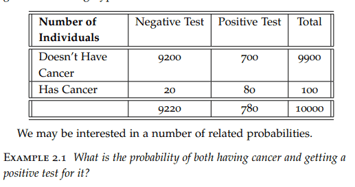
统计代写|统计推断代写Statistical inference代考|Student-t-test

Posted on 2023年5月23日2023年5月23日 by statistics-lab

如果你也在怎样代写统计推断Statistical Inference 这个学科遇到相关的难题，请随时右上角联系我们的24/7代写客服。统计推断Statistical Inference是利用数据分析来推断概率基础分布的属性的过程。推断性统计分析推断人口的属性，例如通过测试假设和得出估计值。假设观察到的数据集是从一个更大的群体中抽出的。

统计推断Statistical Inference（可以与描述性统计进行对比。描述性统计只关注观察到的数据的属性，它并不依赖于数据来自一个更大的群体的假设。在机器学习中，推理一词有时被用来代替 “通过评估一个已经训练好的模型来进行预测”；在这种情况下，推断模型的属性被称为训练或学习（而不是推理），而使用模型进行预测被称为推理（而不是预测）；另见预测推理。

statistics-lab™ 为您的留学生涯保驾护航在代写统计推断Statistical inference方面已经树立了自己的口碑, 保证靠谱, 高质且原创的统计Statistics代写服务。我们的专家在代写统计推断Statistical inference代写方面经验极为丰富，各种代写统计推断Statistical inference相关的作业也就用不着说。

统计代写|统计推断代写Statistical inference代考|Student-t-test

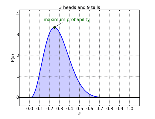
When we are not given the uncertainty of the measurements, $\sigma$, and the data are insufficient to estimate the uncertainty, then we need to estimate both the “true” value, $\mu$, and the uncertainty. This leads to a wider credible range for the “true” value. We can apply the same testing procedure, by looking at the $95 \%$ credible region to see if it includes zero, but this time the posterior distribution we use comes from the so-called Student- $t$ distribution.
1 For $N$ independent observations, we still have the best estimate of the “true” value given by the sample mean
$$
\hat{\mu}=\frac{x_1+x_2+\cdots+x_N}{N}
$$
2 The best estimate of the uncertainty of a single measurement is given by the sample standard deviation
$$
\hat{\sigma}=S
$$
where $S$ is the sample standard deviation
$$
S^2=\frac{1}{N-1}\left(\left(x_1-\bar{x}\right)^2+\cdots+\left(x_N-\bar{x}\right)^2\right)
$$
3 The credible region is determined by the $95 \%$ interval of the posterior, Student- $t$ distribution, of the following form
$$
\text { Student }_{\mathrm{dof}=N-1}(\bar{x}, S / \sqrt{N})
$$
4 Test to see if the credible range includes zero.
5 If so, then the test passes, and we can be reasonably confident that the parameter is non-zero – that the effect is real.
6 If the test fails, i.e. the credible range does not include zero, then under the model the possibility of a zero-effect cannot be reasonably excluded.

统计代写|统计推断代写Statistical inference代考|Model Construction

If we assume a model that states that there is a “true” value and the variation from this “true” value caused by some unknown process, but with known magnitude, $\sigma$,
$$
\text { data }=\text { true value }+\operatorname{Normal}(\text { mean }=\mathrm{o}, \text { known } \sigma)
$$
or equivalently
$$
\text { data }=\operatorname{Normal}(\text { mean=true value, known } \sigma)
$$
we can get the best estimate and uncertainty in that estimate from the following procedure, Using the normal approximation to the Student-T distribution (Section 7.4):
$$
\hat{\mu}=\bar{x} \pm k \cdot S / \sqrt{N}
$$
where the symbols in this equation are
1 the number of data points, $N$.
2 the best estimate for the true value, $\hat{\mu}$, is given by the sample mean, $\bar{x}$ :
$$
\begin{aligned}
\bar{x} & ==\frac{x_1+x_2+\cdots+x_N}{N} \
& =\frac{3.133 \mathrm{~g}+3.083 \mathrm{~g}+\cdots+3.093 \mathrm{~g}}{15} \
& =3.100 \mathrm{~g}
\end{aligned}
$$
3 The uncertainty is directly related to the sample standard deviation, $S:$
$$
\begin{aligned}
S & =\sqrt{\frac{\left(x_1-\bar{x}\right)^2+\left(x_2-\bar{x}\right)^2+\cdots+\left(x_N-\bar{x}\right)^2}{N-1}} \
& =\sqrt{\frac{(3.133 \mathrm{~g}-3.100 \mathrm{~g})^2+(3.083-3.100 \mathrm{~g})^2+\cdots+(3.093-3.100 \mathrm{~g})^2}{14}} \
& =0.0278 \mathrm{~g}
\end{aligned}
$$
4 The scale factor, $k$, adjusts for the small number of data points there is more uncertainty in our estimate when there are fewer data points:

$$
\begin{aligned}
k & =1+\frac{20}{N^2} \
& =1+\frac{20}{15^2} \
& =1.0889
\end{aligned}
$$
Finally, we have the best estimate and uncertainty for the pennies in this dataset:
$$
\begin{aligned}
\hat{\mu} & =\bar{x} \pm k \cdot S / \sqrt{N} \
& =3.100 \mathrm{~g} \pm 1.0889 \cdot 0.0278 \mathrm{~g} / \sqrt{15} \
& =3.100 \mathrm{~g} \pm 0.0078 \mathrm{~g}
\end{aligned}
$$

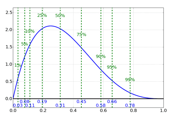
or, as a $99 \%$ credible range ( 3 times the uncertainty written above), we have, (see also Figure 9.4)
$$
\begin{aligned}
99 \% \text { CI for } \mu & =3.100 \mathrm{~g} \pm 3 \times 0.0078 \mathrm{~g} \
& =[3.077 \mathrm{~g}, 3.124 \mathrm{~g}]
\end{aligned}
$$

统计推断代考

统计代写|统计推断代写Statistical inference代考|Student-t-test

当我们没有给出测量的不确定度$\sigma$，并且数据不足以估计不确定度时，那么我们需要估计“真实”值$\mu$和不确定度。这导致“真实”值的可信范围更大。我们可以应用相同的测试程序，通过查看$95 \%$可信区域，看看它是否包含零，但这次我们使用的后验分布来自所谓的Student- $t$分布。
1对于$N$独立观测，我们仍然有样本均值给出的“真实”值的最佳估计
$$
\hat{\mu}=\frac{x_1+x_2+\cdots+x_N}{N}
$$
单次测量的不确定度的最佳估计是由样本标准偏差给出的
$$
\hat{\sigma}=S
$$
其中$S$是样本标准差
$$
S^2=\frac{1}{N-1}\left(\left(x_1-\bar{x}\right)^2+\cdots+\left(x_N-\bar{x}\right)^2\right)
$$
可信区域由以下形式的后验Student- $t$分布的$95 \%$区间确定
$$
\text { Student }_{\mathrm{dof}=N-1}(\bar{x}, S / \sqrt{N})
$$
4测试可信范围是否包括零。
如果是这样，那么测试通过了，我们可以合理地确信参数是非零的-效果是真实的。
如果检验不通过，即可信范围不包括零，则在该模型下不能合理地排除零效应的可能性。

统计代写|统计推断代写Statistical inference代考|Model Construction

如果我们假设一个模型表明存在一个“真实”值，并且这个“真实”值的变化是由某些未知过程引起的，但具有已知的大小，$\sigma$，
$$
\text { data }=\text { true value }+\operatorname{Normal}(\text { mean }=\mathrm{o}, \text { known } \sigma)
$$
或者等价地
$$
\text { data }=\operatorname{Normal}(\text { mean=true value, known } \sigma)
$$
使用Student-T分布的正态近似(第7.4节)，我们可以通过以下步骤获得最佳估计和该估计的不确定性:
$$
\hat{\mu}=\bar{x} \pm k \cdot S / \sqrt{N}
$$
方程中的符号在哪里
1 .数据点数，$N$。
2真实值的最佳估计值$\hat{\mu}$由样本均值$\bar{x}$给出:
$$
\begin{aligned}
\bar{x} & ==\frac{x_1+x_2+\cdots+x_N}{N} \
& =\frac{3.133 \mathrm{~g}+3.083 \mathrm{~g}+\cdots+3.093 \mathrm{~g}}{15} \
& =3.100 \mathrm{~g}
\end{aligned}
$$
3不确定度与样品标准差直接相关，$S:$
$$
\begin{aligned}
S & =\sqrt{\frac{\left(x_1-\bar{x}\right)^2+\left(x_2-\bar{x}\right)^2+\cdots+\left(x_N-\bar{x}\right)^2}{N-1}} \
& =\sqrt{\frac{(3.133 \mathrm{~g}-3.100 \mathrm{~g})^2+(3.083-3.100 \mathrm{~g})^2+\cdots+(3.093-3.100 \mathrm{~g})^2}{14}} \
& =0.0278 \mathrm{~g}
\end{aligned}
$$
4 .比例因子$k$针对少量数据点进行调整，当数据点较少时，我们的估计存在更大的不确定性:

$$
\begin{aligned}
k & =1+\frac{20}{N^2} \
& =1+\frac{20}{15^2} \
& =1.0889
\end{aligned}
$$
最后，我们对这个数据集中的便士有了最好的估计和不确定性:
$$
\begin{aligned}
\hat{\mu} & =\bar{x} \pm k \cdot S / \sqrt{N} \
& =3.100 \mathrm{~g} \pm 1.0889 \cdot 0.0278 \mathrm{~g} / \sqrt{15} \
& =3.100 \mathrm{~g} \pm 0.0078 \mathrm{~g}
\end{aligned}
$$

或者，作为$99 \%$可信范围(上述不确定性的3倍)，我们有，(参见图9.4)
$$
\begin{aligned}
99 \% \text { CI for } \mu & =3.100 \mathrm{~g} \pm 3 \times 0.0078 \mathrm{~g} \
& =[3.077 \mathrm{~g}, 3.124 \mathrm{~g}]
\end{aligned}
$$

统计代写|统计推断代写Statistical inference代考请认准statistics-lab™

统计代写请认准statistics-lab™. statistics-lab™为您的留学生涯保驾护航。

金融工程代写

金融工程是使用数学技术来解决金融问题。金融工程使用计算机科学、统计学、经济学和应用数学领域的工具和知识来解决当前的金融问题，以及设计新的和创新的金融产品。

非参数统计代写

非参数统计指的是一种统计方法，其中不假设数据来自于由少数参数决定的规定模型；这种模型的例子包括正态分布模型和线性回归模型。

广义线性模型代考

广义线性模型（GLM）归属统计学领域，是一种应用灵活的线性回归模型。该模型允许因变量的偏差分布有除了正态分布之外的其它分布。

术语广义线性模型（GLM）通常是指给定连续和/或分类预测因素的连续响应变量的常规线性回归模型。它包括多元线性回归，以及方差分析和方差分析（仅含固定效应）。

有限元方法代写

有限元方法（FEM）是一种流行的方法，用于数值解决工程和数学建模中出现的微分方程。典型的问题领域包括结构分析、传热、流体流动、质量运输和电磁势等传统领域。

有限元是一种通用的数值方法，用于解决两个或三个空间变量的偏微分方程（即一些边界值问题）。为了解决一个问题，有限元将一个大系统细分为更小、更简单的部分，称为有限元。这是通过在空间维度上的特定空间离散化来实现的，它是通过构建对象的网格来实现的：用于求解的数值域，它有有限数量的点。边界值问题的有限元方法表述最终导致一个代数方程组。该方法在域上对未知函数进行逼近。[1] 然后将模拟这些有限元的简单方程组合成一个更大的方程系统，以模拟整个问题。然后，有限元通过变化微积分使相关的误差函数最小化来逼近一个解决方案。

tatistics-lab作为专业的留学生服务机构，多年来已为美国、英国、加拿大、澳洲等留学热门地的学生提供专业的学术服务，包括但不限于Essay代写，Assignment代写，Dissertation代写，Report代写，小组作业代写，Proposal代写，Paper代写，Presentation代写，计算机作业代写，论文修改和润色，网课代做，exam代考等等。写作范围涵盖高中，本科，研究生等海外留学全阶段，辐射金融，经济学，会计学，审计学，管理学等全球99%专业科目。写作团队既有专业英语母语作者，也有海外名校硕博留学生，每位写作老师都拥有过硬的语言能力，专业的学科背景和学术写作经验。我们承诺100%原创，100%专业，100%准时，100%满意。

随机分析代写

随机微积分是数学的一个分支，对随机过程进行操作。它允许为随机过程的积分定义一个关于随机过程的一致的积分理论。这个领域是由日本数学家伊藤清在第二次世界大战期间创建并开始的。

时间序列分析代写

随机过程，是依赖于参数的一组随机变量的全体，参数通常是时间。随机变量是随机现象的数量表现，其时间序列是一组按照时间发生先后顺序进行排列的数据点序列。通常一组时间序列的时间间隔为一恒定值（如1秒，5分钟，12小时，7天，1年），因此时间序列可以作为离散时间数据进行分析处理。研究时间序列数据的意义在于现实中，往往需要研究某个事物其随时间发展变化的规律。这就需要通过研究该事物过去发展的历史记录，以得到其自身发展的规律。

回归分析代写

多元回归分析渐进（Multiple Regression Analysis Asymptotics）属于计量经济学领域，主要是一种数学上的统计分析方法，可以分析复杂情况下各影响因素的数学关系，在自然科学、社会和经济学等多个领域内应用广泛。

MATLAB代写

MATLAB 是一种用于技术计算的高性能语言。它将计算、可视化和编程集成在一个易于使用的环境中，其中问题和解决方案以熟悉的数学符号表示。典型用途包括：数学和计算算法开发建模、仿真和原型制作数据分析、探索和可视化科学和工程图形应用程序开发，包括图形用户界面构建MATLAB 是一个交互式系统，其基本数据元素是一个不需要维度的数组。这使您可以解决许多技术计算问题，尤其是那些具有矩阵和向量公式的问题，而只需用 C 或 Fortran 等标量非交互式语言编写程序所需的时间的一小部分。MATLAB 名称代表矩阵实验室。MATLAB 最初的编写目的是提供对由 LINPACK 和 EISPACK 项目开发的矩阵软件的轻松访问，这两个项目共同代表了矩阵计算软件的最新技术。MATLAB 经过多年的发展，得到了许多用户的投入。在大学环境中，它是数学、工程和科学入门和高级课程的标准教学工具。在工业领域，MATLAB 是高效研究、开发和分析的首选工具。MATLAB 具有一系列称为工具箱的特定于应用程序的解决方案。对于大多数 MATLAB 用户来说非常重要，工具箱允许您学习和应用专业技术。工具箱是 MATLAB 函数（M 文件）的综合集合，可扩展 MATLAB 环境以解决特定类别的问题。可用工具箱的领域包括信号处理、控制系统、神经网络、模糊逻辑、小波、仿真等。

R语言代写	问卷设计与分析代写
PYTHON代写	回归分析与线性模型代写
MATLAB代写	方差分析与试验设计代写
STATA代写	机器学习/统计学习代写
SPSS代写	计量经济学代写
EVIEWS代写	时间序列分析代写
EXCEL代写	深度学习代写
SQL代写	各种数据建模与可视化代写

统计代写|统计推断代写Statistical inference代考|Marginalization

Posted on 2023年5月23日2023年5月23日 by statistics-lab

统计代写|统计推断代写Statistical inference代考|Marginalization

In Section 1.4 we introduced the concept of marginalization, and in Section 2.1 we performed a discrete example of this. In that section it was seen as simply a consequence of the sum and product rules. It was a way of taking a probability that depended on several factors, and eliminating all but the single factor we’re interested in. If we have a continuous distribution, this process involves calculus and we will not cover it in detail, but it is the same process. In the case of the distribution above, we have a distribution over a single variable, like $\operatorname{Beta}(\theta \mid h, t)$. Imagine that we have a distribution that depends on two parameters,
$$
\operatorname{MyDist}(\theta, \xi)
$$
which specifies the probability of an event given each combination of the parameters, $\theta$ and $\xi$. We’d have to do a three-dimensional plot to visualize this. Many times, however, we want just the probability of one of the single parameters. In those cases we will write
$$
P(\theta) \sim[\operatorname{MyDist}(\theta, \xi)]_{\text {marginalize over } \xi}
$$
where we are “summing” over all the values of the other parameters, leaving the details to the mathematicians, and simply using the result.

Likewise we can marginalize the parameter $\theta$ to get the distribution of the other variable.
$$
P(\xi) \sim[\operatorname{MyDist}(\theta, \xi)]_{\text {marginalize over } \theta}
$$

统计代写|统计推断代写Statistical inference代考|Binomial and Beta Distributions

In Chapter 6 (Introduction to Parameter Estimation on page 121) we estimated the chance, $\theta$, that a bent coin would come up heads by combining a uniform prior for $\theta$ (i.e. all possible values are a-priori equally likely) and a binomial likelihood (i.e. given $\theta$, what is the probability of the data). This resulted in a Beta distribution for the posterior probability for $\theta$.
Notice what the procedure of Bayes’ Recipe is and how the Bayesian inference works here.
1 Specify the prior probabilities for the models being considered
We want to estimate a quantity (which we label as $\theta$ ), but begin with absolutely no knowledge of its value – we have a uniform prior probability.
2 Write the top of Bayes’ Rule for all models being considered
We construct a model for how different possible values of $\theta$ influence the outcome – a model we call the likelihood. In the case of the bent coin, the likelihood model is a binomial model, and describes the probability of flipping heads or tails given how bent the coin is (i.e. given $\theta$ ).
3 Put in the likelihood and prior values
4 Add these values for all models
5 Divide each of the values by this sum, $K$, to get the final probabilities
Once we observe data, we can combine the prior and the model or likelihood using the Bayes’ recipe, and obtain the posterior distribution for the unknown value, $\theta$, giving us the probability for each value, now updated with our new observations.

统计推断代考

统计代写|统计推断代写Statistical inference代考|Marginalization

在1.4节中，我们介绍了边缘化的概念，在2.1节中，我们执行了一个离散的例子。在那一节中，它被看作是简单的求和和乘积规则的结果。这是一种取概率的方法它取决于几个因素，然后剔除所有我们感兴趣的因素。如果我们有一个连续分布，这个过程涉及微积分，我们不会详细讲，但它是相同的过程。在上述分布的情况下，我们有一个单一变量的分布，如$\operatorname{Beta}(\theta \mid h, t)$。假设我们有一个依赖于两个参数的分布，
$$
\operatorname{MyDist}(\theta, \xi)
$$
它指定给定参数$\theta$和$\xi$的每种组合的事件的概率。我们需要做一个三维图来形象化。然而，很多时候，我们只想要单个参数中的一个的概率。在这种情况下，我们会写
$$
P(\theta) \sim[\operatorname{MyDist}(\theta, \xi)]_{\text {marginalize over } \xi}
$$
我们对其他参数的所有值进行“求和”，将细节留给数学家，并简单地使用结果。

同样，我们可以将参数$\theta$边缘化，从而得到另一个变量的分布。
$$
P(\xi) \sim[\operatorname{MyDist}(\theta, \xi)]_{\text {marginalize over } \theta}
$$

统计代写|统计推断代写Statistical inference代考|Binomial and Beta Distributions

在第6章(121页参数估计的介绍)中，我们通过结合$\theta$的统一先验(即所有可能的值都是先验的等可能)和二项似然(即给定$\theta$，数据的概率是什么)来估计概率$\theta$，即一枚弯曲的硬币将出现正面。这导致了$\theta$后验概率的Beta分布。
注意贝叶斯公式的过程是什么以及贝叶斯推理是如何工作的。
指定所考虑的模型的先验概率
我们想要估计一个量(我们标记为$\theta$)，但是在完全不知道它的值的情况下开始——我们有一个均匀的先验概率。
写下所有考虑的模型的贝叶斯规则的顶部
我们构建了一个模型，说明$\theta$的不同可能值如何影响结果——我们称之为可能性模型。在硬币弯曲的情况下，可能性模型是一个二项模型，并描述了给定硬币弯曲程度的抛掷正面或反面的概率(即给定$\theta$)。
输入可能性和先验值
4将所有模型的值相加
5将每个值除以这个和$K$，得到最终的概率
一旦我们观察到数据，我们可以使用贝叶斯配方将先验和模型或似然结合起来，并获得未知值的后验分布$\theta$，为我们提供每个值的概率，现在用我们的新观测值更新。

统计代写请认准statistics-lab™. statistics-lab™为您的留学生涯保驾护航。

金融工程代写

非参数统计代写

非参数统计指的是一种统计方法，其中不假设数据来自于由少数参数决定的规定模型；这种模型的例子包括正态分布模型和线性回归模型。

广义线性模型代考

广义线性模型（GLM）归属统计学领域，是一种应用灵活的线性回归模型。该模型允许因变量的偏差分布有除了正态分布之外的其它分布。

有限元方法代写

随机分析代写

时间序列分析代写

回归分析代写

MATLAB代写

R语言代写	问卷设计与分析代写
PYTHON代写	回归分析与线性模型代写
MATLAB代写	方差分析与试验设计代写
STATA代写	机器学习/统计学习代写
SPSS代写	计量经济学代写
EVIEWS代写	时间序列分析代写
EXCEL代写	深度学习代写
SQL代写	各种数据建模与可视化代写

统计代写|统计推断代写Statistical inference代考|Priors versus Data

Posted on 2023年5月23日2023年5月23日 by statistics-lab

统计代写|统计推断代写Statistical inference代考|Priors versus Data

It is instructive to pause and look at this example one flip at a time, to see how the probability and thus our state of knowledge adjusts as we collect more data. In Figure 6.3 we see the result of our procedure when there is no data (i.e. our initial, prior probabilities) and when we’ve flipped once and then again, both times tails. The curve for “no data” is the same as the prior probability, and in this case all models are equally likely. When the first tails is observed, the model which states that heads are certain (i.e. coin 10) goes to zero probability because coin 10 cannot flip tails. ${ }^2$. At this point we know that it is impossible for us to be flipping coin 10. We see also that the highnumbered coins (i.e. the ones with high probability of flipping heads) have greatly reduced probability while we’ve seen only tails.
As more tails are observed, the probability for the lower models is increased. As we flip more tails we become more confident in the lower-number models. Because at this point we haven’t flipped any heads, the model o still has non-zero probability – it is still possible that we are holding a coin that cannot flip heads.
When we continue with the next few flips (Figure 6.4) we encounter our first heads on the fourth flip. At this point the model which states that heads are impossible (i.e coin o) goes to zero probability. Finally, across our entire data set (Figure 6.5) we see that the curve gets narrower, where more of the probability falls on only a few of the models and the other models become less and less likely. With only 12 data points, there is still a lot of uncertainty in which model – several models have reasonably high probability values. We still can rule out a few models confidently (like coins o, 6, 7,8, 9, and 10). We are most confident in coins 2 and 3 , with the most probability.

统计代写|统计推断代写Statistical inference代考|Moving Toward the Continuous

There is a practical problem that we face at this point, when we consider a generic bent coin. Perhaps it doesn’t fit in one of the 11 models considered, falling somewhere in between, for example with $P$ (heads) $=0.132464$. Ones’ first thought might be to include one thousand coins or one million coins instead of the 11 we’ve considered so far, so we could have coin 132464, coin 132465, coin 132466, etc… Although this can be done, we run into two problems
1 Because we are dealing with so many models, the probability associated with any single model gets very small – and gets smaller with the more models you consider
2 We can’t practically distinguish between models such as $P$ (heads) = 0.132464 and $P$ (heads) $=0.132465$ (the last digit is different here)

In order to solve both of these problems mathematically, we introduce the concept of a continuous distribution. We start by labeling the model with a continuous number rather than an integer. In our present case it makes sense to label the model with the probability that the coin flips heads. We’ll call this label $\theta$, and it will have a value between o (heads are impossible) and I (heads are certain) and can take on any value in between. Because we now have an infinite number of labels, we have two consequences:
1 We can’t simply add up all the probabilities to get our value of $K$ to make everything add up to 1 . Instead, we look at areas under the curve and make sure the entire area equals 1.
2 Because, with distributions, areas under the curve (and not the values of the distribution itself) are the probabilities, we can only speak about ranges of values. For example, we can speak meaningfully about the probability of $\theta$ between o.3 and o.4 (i.e. $P(0.3<\theta<0.4))$. When we write down something like $P(\theta)=1$ we’re not talking about a probability of a single label but rather the magnitude of the distribution at that label, $\theta$.

统计推断代考

统计代写|统计推断代写Statistical inference代考|Priors versus Data

暂停一下，一次看一次这个例子，看看随着我们收集更多的数据，概率和我们的知识状态是如何调整的，这是有指导意义的。在图6.3中，我们看到了没有数据(即初始先验概率)和一次又一次抛硬币的结果，两次都是反面。“无数据”的曲线与先验概率相同，在这种情况下，所有模型都是等可能的。当观察到第一次反面时，声称正面是确定的模型(即第10枚硬币)的概率变为零，因为第10枚硬币不能掷出反面。${} ^ 2美元。此时，我们知道抛硬币10是不可能的。我们还看到，高编号硬币(即有高概率抛掷正面的硬币)的概率大大降低，而我们只看到反面。
随着观察到更多的反面，较低模型的概率增加。反面掷得越多，我们就越相信次数较少的模型。因为在这一点上，我们还没有抛过任何正面，模型0仍然有非零概率-，仍然有可能我们拿着的硬币不能抛正面。
当我们继续进行接下来的几次投掷(图6.4)时，我们在第四次投掷时遇到了第一次正面。此时，认为头像不可能出现的模型(即硬币0)的概率变为零。最后，纵观我们的整个数据集(图6.5)，我们看到曲线变得越来越窄，其中更多的概率落在少数模型上，而其他模型的可能性越来越小。在只有12个数据点的情况下，哪个模型仍然存在很多不确定性——有几个模型具有相当高的概率值。我们仍然可以自信地排除一些模型(如硬币0、6、7、8、9和10)。我们对硬币2和3最有信心，概率最大。

统计代写|统计推断代写Statistical inference代考|Moving Toward the Continuous

在这一点上，我们面临一个实际问题，当我们考虑一个一般的弯曲硬币时。也许它不适合所考虑的11个模型中的一个，落在两者之间的某个地方，例如$P$(正面)$=0.132464$。人们的第一个想法可能是包括1000枚或100万枚硬币，而不是我们目前考虑的11枚硬币，所以我们可以有硬币132464，硬币132465，硬币132466，等等
因为我们要处理的模型太多了，与任何一个模型相关的概率都变得非常小，而且随着你考虑的模型越多，概率就越小
2 .我们实际上无法区分$P$(正面)= 0.132464和$P$(正面)$=0.132465$(这里的最后一位数字不同)这样的模型。

为了从数学上解决这两个问题，我们引入了连续分布的概念。我们首先用连续数而不是整数标记模型。在我们目前的情况下，用硬币正面朝上的概率来标记模型是有意义的。我们称这个标签为$\theta$，它的值介于0(不可能出现正面)和I(正面是肯定的)之间，可以取这两者之间的任何值。因为我们现在有无限多的标签，我们有两个结果:
我们不能简单地把所有的概率加起来，使K的值等于1。相反，我们看曲线下的面积，确保整个面积等于1。
因为，对于分布，曲线下的面积(而不是分布本身的值)是概率，我们只能谈论值的范围。例如，我们可以有意义地讨论$\theta$在0.3和0.4之间的概率(例如$ P(0.3 < \θ< 0.4))。当我们写下P(\ θ)=1时我们不是在讨论单个标签的概率，而是在该标签处分布的大小。

统计代写请认准statistics-lab™. statistics-lab™为您的留学生涯保驾护航。

金融工程代写

非参数统计代写

非参数统计指的是一种统计方法，其中不假设数据来自于由少数参数决定的规定模型；这种模型的例子包括正态分布模型和线性回归模型。

广义线性模型代考

广义线性模型（GLM）归属统计学领域，是一种应用灵活的线性回归模型。该模型允许因变量的偏差分布有除了正态分布之外的其它分布。

有限元方法代写

随机分析代写

时间序列分析代写

回归分析代写

MATLAB代写

R语言代写	问卷设计与分析代写
PYTHON代写	回归分析与线性模型代写
MATLAB代写	方差分析与试验设计代写
STATA代写	机器学习/统计学习代写
SPSS代写	计量经济学代写
EVIEWS代写	时间序列分析代写
EXCEL代写	深度学习代写
SQL代写	各种数据建模与可视化代写

统计代写|统计推断代写Statistical inference代考|Visualization of Data

Posted on 2023年5月12日2023年5月12日 by statistics-lab

统计代写|统计推断代写Statistical inference代考|Visualization of Data

There are two main methods of visualizing data, and several others that are related to these methods. In this section we introduce just two, histograms and scatter plots, and we will use these throughout the text.
Histograms
Histograms are a way of summarizing data, when presenting the entire data set is impractical, or where some understanding of the data is made clearer by summarizing. The histogram plot is done with the following steps:
1 Choose a number of bins to divide the data.
2 Count up the data that fall into each bin
3 Make a bar plot, or a scatter plot to present the data.
The following is an example with a small data set. The process of binning and counting is often done by computer, but it is instructive to perform the process by hand a few times in order to understand what the results are.

Table 3.3 shows a collection of 106 heights (in centimeters) of the male students in a class’. As a collection of numbers it is relatively opaque, but as a histogram it is clearer.

From this histogram, we can immediately observe several quantities which summarize their data:
1 The average value (around the middle) should be around $175 \mathrm{~cm}$. The actual value can be calculated from the data, as
$$
\bar{x}=\frac{177.8+160.0+\cdots+180.34+183.0}{106}=178.83
$$
2 The range of the data is around $155 \mathrm{~cm}$ up to about $205 \mathrm{~cm}$. Again we can be more precise, and find the minimum of the data (154.94 $\mathrm{cm}$ ) and the maximum $(200 \mathrm{~cm}$ ) but the histogram picture yields an approximate value instantly.
3 The values are roughly symmetric about the mean (i.e. average) value. This can give us a clue concerning how to model the data.
What is quite clear is that it is far easier to deal with a histogram, as above, than find the same information from the table of numbers.

统计代写|统计推断代写Statistical inference代考|Computer Examples

This section summarizes how to make histograms and scatter plots with the computer software.
Histograms
from sie import *
Load a sample data set, and select only the Male data…
$$
\begin{aligned}
& \text { data=load_data (‘data/survey .csv’) } \
& \text { male_data=data [data [‘Sex’]== ‘Male’] }
\end{aligned}
$$
select only the height data, and drop the missing data (na)…
$$
\text { male_height }=\text { male_data [ ‘Height’]. dropna() }
$$
make the histogram
$$
\begin{aligned}
& \text { hist (male_height, bins }=20) \
& \text { xlabel (‘Height [cm]’) } \
& \text { ylabel (‘Number of People’) }
\end{aligned}
$$
$

data=load_data(‘data/survey.csv’)
male_data=data $[$ data [‘Sex’ $]==$ ‘Male’]
select only the height and the width of writing hand data, and drop the missing data (na)…
subdata=male_data [[ ‘Height’, ‘Wr.Hnd’]].dropna ()
height=subdata [‘Height’]
wr_hand=subdata [ ‘Wr.Hnd’]
plot the data
plot (height,wr_hand, ‘o’)
ylabel (‘Writing Hand Span [cm]’)
xlabel (‘Height [cm]’)
$

统计推断代考

统计代写|统计推断代写Statistical inference代考|Visualization of Data

有两种主要的数据可视化方法，以及与这些方法相关的其他几种方法。在本节中，我们只介绍两种，直方图和散点图，我们将在整个文本中使用它们。
直方图
当呈现整个数据集是不切实际的，或者通过汇总可以更清楚地理解数据时，直方图是一种汇总数据的方式。直方图的绘制步骤如下:
1选择若干个bin对数据进行划分。
把每个箱子里的数据加起来
制作条形图或散点图来表示数据。
下面是一个小数据集的例子。装箱和计数的过程通常是由计算机完成的，但为了了解结果是什么，手工执行几次这个过程是有指导意义的。

表3.3是某班级男生身高(厘米)106的汇总。作为一组数字，它相对不透明，但作为一个直方图，它更清晰。

从这个直方图中，我们可以立即观察到总结其数据的几个量:
1平均值(中间左右)应在$175 \mathrm{~cm}$左右。实际值可由数据计算得出，为
$$
\bar{x}=\frac{177.8+160.0+\cdots+180.34+183.0}{106}=178.83
$$
2数据范围在$155 \mathrm{~cm}$ ～ $205 \mathrm{~cm}$左右。同样，我们可以更精确地找到数据的最小值(154.94 $\mathrm{cm}$)和最大值$(200 \mathrm{~cm}$)，但直方图立即产生一个近似值。
这些值大致对称于平均值(即平均值)。这可以给我们一个关于如何对数据建模的线索。
很明显，处理直方图要比从数字表中找到相同的信息容易得多。

统计代写|统计推断代写Statistical inference代考|Computer Examples

本节总结了如何用计算机软件制作直方图和散点图。
直方图
源自sie import *
加载一个样本数据集，并只选择Male数据…
$$
\begin{aligned}
& \text { data=load_data (‘data/survey .csv’) } \
& \text { male_data=data [data [‘Sex’]== ‘Male’] }
\end{aligned}
$$
只选择高度数据，并删除缺失的数据(na)…
$$
\text { male_height }=\text { male_data [ ‘Height’]. dropna() }
$$
制作直方图
$$
\begin{aligned}
& \text { hist (male_height, bins }=20) \
& \text { xlabel (‘Height [cm]’) } \
& \text { ylabel (‘Number of People’) }
\end{aligned}
$$
$

data=load_data(‘data/survey.csv’)
male_data=data $ [$ data [‘Sex’ $]==$ ‘Male’]
select only the height and the width of writing hand data, and drop the missing data (na)…
subdata=male_data [[ ‘Height’, ‘Wr.Hnd’]].dropna ()
height=subdata [‘Height’]
wr_hand=subdata [ ‘Wr.Hnd’]
plot the data
plot (height,wr_hand, ‘o’)
ylabel (‘Writing Hand Span [cm]’)
xlabel (‘Height [cm]’)
$

统计代写请认准statistics-lab™. statistics-lab™为您的留学生涯保驾护航。

金融工程代写

非参数统计代写

非参数统计指的是一种统计方法，其中不假设数据来自于由少数参数决定的规定模型；这种模型的例子包括正态分布模型和线性回归模型。

广义线性模型代考

广义线性模型（GLM）归属统计学领域，是一种应用灵活的线性回归模型。该模型允许因变量的偏差分布有除了正态分布之外的其它分布。

有限元方法代写

随机分析代写

时间序列分析代写

回归分析代写

MATLAB代写

R语言代写	问卷设计与分析代写
PYTHON代写	回归分析与线性模型代写
MATLAB代写	方差分析与试验设计代写
STATA代写	机器学习/统计学习代写
SPSS代写	计量经济学代写
EVIEWS代写	时间序列分析代写
EXCEL代写	深度学习代写
SQL代写	各种数据建模与可视化代写

统计代写|统计推断代写Statistical inference代考|Three Doors with Information

Posted on 2023年5月12日2023年5月12日 by statistics-lab

统计代写|统计推断代写Statistical inference代考|Three Doors with Information

We return to the three-door case with a slight variation
ExAmpLE 2.17 Suppose you’re on a game show, and you’re given the choice of three doors: Behind one door is a car; behind the others, goats. You pick a door, say No. I (but the door is not opened), and the host, who knows what’s behind the doors, says that another door, say No. 3, has a o\% chance of having a car, and that the remaining door (that you haven’t chosen – i.e door No. 2) has a $66 \%$ of having the car. He then says to you, “Do you want to pick door No. 2?” Is it to your advantage to switch your choice?
In this case, switching to door No. 3 would be ridiculous – we know the car isn’t there, because the (honest) host knows that it is not there. The host also has told us that there is a $66 \%$ chance of the car behind door No. 2, and thus we have $P$ (car behind No. 1 ) $=0.34$ and $P($ car behind No. 2$)=0.66$ and it is better to switch to door No. 2.

It isn’t the number of choices that is important, it is the information we have about those choices. When you have no information, we assign equal probabilities. When we have information, we can assign non-equal probabilities.

统计代写|统计推断代写Statistical inference代考|Back to our original problem, we have

EXAMPLE 2.18 Suppose you’re on a game show, and you’re given the choice of three doors: behind one door is a car; behind the others, goats. You pick a door, say No. I (but the door is not opened), and the host, who knows what’s behind the doors, opens another door, say No. 3, which has a goat. He then says to you, “Do you want to change your choice to door No. 2?” Is it to your advantage or disadvantage to switch your choice, or does it matter whether you switch your choice or not?
The key part is that, no matter what happens,
I the host never opens your door
2 the host always opens a door with a goat
Given that your first choice, with three equal probability choices (i.e. you have no information about any of the choices), we expect to be correct only about $33 \%$ of the time. If we happened to get lucky with our first choice, then the host has a pick of two doors with goats and has some freedom. If we happened to get unlucky with our first choice (and there is a goat behind it), then the host has no freedom at all, because there is only one remaining door with a goat. So, about $66 \%$ of the time the host is forced to reveal some of his information, because the door he leaves closed (other than your door) must have the car. Thus, $66 \%$ of the time the host is telling you where the car is, just a little indirectly.

Formally, we need to involve model comparison, so we postpone this particular analysis until Section 5.4.

统计推断代考

统计代写|统计推断代写Statistical inference代考|Three Doors with Information

我们回到三门的情况下略有变化
例2.17假设你正在参加一个游戏节目，你被要求从三扇门中做出选择:一扇门后面是一辆车;在其他动物后面的是山羊。你选了一扇门，说不。我(但门没有打开)和知道门后面是什么的主持人说，另一扇门，比如3号门，有0 %的几率有车，而剩下的一扇门(你没有选择的，也就是2号门)有66 %的几率有车。然后他对你说:“你想选2号门吗?”改变你的选择对你有利吗?
在这种情况下，切换到3号门将是荒谬的-我们知道车不在那里，因为(诚实的)主人知道它不在那里。主持人还告诉我们，2号门后面的车有66%的可能性，因此我们有$P$(1号门后面的车)$=0.34$和$P$(2号门后面的车)=0.66$，最好换成2号门。

重要的不是选择的数量，而是我们掌握的关于这些选择的信息。当你没有信息时，我们分配相等的概率。当我们有信息时，我们可以分配非等概率。

统计代写|统计推断代写Statistical inference代考|Back to our original problem, we have

例2.18假设你正在参加一个游戏节目，你被要求从三扇门中做出选择:一扇门后面是一辆车;在其他动物后面的是山羊。你选了一扇门，说不。我(但门没有打开)和主人(他知道门后面是什么)打开了另一扇门，比如说3号，里面有一只山羊。然后他对你说:“你想改走2号门吗?”改变你的选择对你是有利还是不利，或者你是否改变你的选择有关系吗?
关键是，无论发生什么，
如果主人从不给你开门
主人总是用山羊开门
考虑到你的第一个选择，有三个等概率的选择(即你没有关于任何选择的信息)，我们预计只有大约33%的时间是正确的。如果我们碰巧幸运地选择了第一个，那么主人可以选择两个带山羊的门，并有一些自由。如果我们的第一个选择碰巧不走运(门后面有一只山羊)，那么主人就完全没有自由了，因为只剩下一扇门上有一只山羊。所以，大约66%的时候主人被迫透露他的一些信息，因为他留下的门关着(除了你的门)一定有车。因此，在66%的时间里，主人会告诉你车在哪里，只是有点间接。

形式上，我们需要涉及模型比较，因此我们将这个特殊的分析推迟到第5.4节。

统计代写请认准statistics-lab™. statistics-lab™为您的留学生涯保驾护航。

金融工程代写

非参数统计代写

非参数统计指的是一种统计方法，其中不假设数据来自于由少数参数决定的规定模型；这种模型的例子包括正态分布模型和线性回归模型。

广义线性模型代考

广义线性模型（GLM）归属统计学领域，是一种应用灵活的线性回归模型。该模型允许因变量的偏差分布有除了正态分布之外的其它分布。

有限元方法代写

随机分析代写

时间序列分析代写

回归分析代写

MATLAB代写

R语言代写	问卷设计与分析代写
PYTHON代写	回归分析与线性模型代写
MATLAB代写	方差分析与试验设计代写
STATA代写	机器学习/统计学习代写
SPSS代写	计量经济学代写
EVIEWS代写	时间序列分析代写
EXCEL代写	深度学习代写
SQL代写	各种数据建模与可视化代写

统计代写|统计推断代写Statistical inference代考|Cancer and Probability

Posted on 2023年5月12日2023年5月12日 by statistics-lab

统计代写|统计推断代写Statistical inference代考|Cancer and Probability

This is perhaps the most important probability question to learn, so we will spend some time covering it here and then cover it again, in a slightly different way, in Section 5.1 on page 109. Imagine we have a population of 10000 people who have been tested for cancer, and we get the following hypothetical data:

We can determine this by simply dividing the person counts from the table
$$
\begin{aligned}
P(\text { cancer and positive test }) & =\frac{# \text { of people with both cancer and positive test }}{\text { total # of people }} \
& =\frac{80}{10000}=0.008
\end{aligned}
$$
Doing this process for every part of the table yields a posterior probability table, giving the probability for every combination of variables (i.e. with cancer and positive test, without cancer and positive test, etc…)

Reading off of the table, we have
$$
P \text { (no cancer and positive test })=0.07
$$
This question, it turns out, is a not very interesting question. The type of question that actually arises in life is the following,

EXAMPLE 2.3 What is the probability of having cancer given a positive test for it?

Here we can perform the calculation in a couple of different ways, to give the (unintuitive) result.

统计代写|统计推断代写Statistical inference代考|Weather

ExAMPLE 2.4 If the probability that it will rain next Saturday is o.25 and the probability that it will rain next Sunday is 0.25 , what is the probability that it will rain during the weekend?
First Solution – Independence
If we assume that Sunday and Saturday weather are independent then the sum-rule (Section 1.4) applies:
$P($ rain Saturday or rain Sunday $)=$
$$
\begin{aligned}
& P(\text { rain Saturday })+P(\text { rain Sunday })-P(\text { rain Saturday and rain Sunday }) \
= & P(\text { rain Saturday })+P(\text { rain Sunday })-P(\text { rain Saturday }) \times P(\text { rain Sunday }) \
= & 0.25+0.25-0.25 \times 0.25=0.4375
\end{aligned}
$$
The diagrams in Figure 1.3 are useful in making this calculation more intuitive, especially the term where we subtract $P$ (rain Saturday) $\times$ $P$ (rain Sunday) because otherwise we over count the double-rain weekends.

Second Solution – Correlation
Is it really reasonable that rain on Saturday and Sunday are independent events? Probably not! It’s probably the case that knowing that it rained on Saturday, then rain on Sunday is more likely. It may also be that if it didn’t rain on Saturday then it will be less likely for rain on Sunday. So we’d have information possibly like:
$$
\begin{aligned}
P(\text { rain Sunday } \mid \text { rain Saturday }) & =0.35 \
P(\text { rain Sunday } \mid \text { not rain Saturday }) & =0.15
\end{aligned}
$$
Knowing this changes the equation as
$$
P(\text { rain Saturday or rain Sunday })=
$$

= P(rain Saturday) + P(rain Sunday) − P(rain Saturday and rain Sunday)

统计推断代考

统计代写|统计推断代写Statistical inference代考|Cancer and Probability

这可能是要学习的最重要的概率问题，所以我们将在这里花一些时间来讨论它，然后在109页的5.1节以稍微不同的方式再次讨论它。假设我们有一万人接受了癌症检测，我们得到以下假设数据:

我们可以通过简单地除以表格中的人数来确定这一点
$$
\begin{aligned}
P(\text { cancer and positive test }) & =\frac{# \text { of people with both cancer and positive test }}{\text { total # of people }} \
& =\frac{80}{10000}=0.008
\end{aligned}
$$
对表格的每个部分进行这个过程，会得到一个后验概率表，给出每个变量组合的概率(例如，有癌症和阳性测试，没有癌症和阳性测试，等等……)

桌上的读数，我们有
$$
P \text { (no cancer and positive test })=0.07
$$
这个问题，其实不是一个很有趣的问题。生活中实际出现的问题类型如下:

例2.3如果癌症检测呈阳性，患癌症的概率是多少?

在这里，我们可以用几种不同的方式执行计算，以给出(不直观的)结果。

统计代写|统计推断代写Statistical inference代考|Weather

如果下星期六下雨的概率是0.25，下星期天下雨的概率是0.25，那么周末下雨的概率是多少?
第一种解决方案-独立
如果我们假设周日和周六的天气是独立的，那么求和规则(第1.4节)适用:
$P($周六下雨，周日下雨$)=$
$$
\begin{aligned}
& P(\text { rain Saturday })+P(\text { rain Sunday })-P(\text { rain Saturday and rain Sunday }) \
= & P(\text { rain Saturday })+P(\text { rain Sunday })-P(\text { rain Saturday }) \times P(\text { rain Sunday }) \
= & 0.25+0.25-0.25 \times 0.25=0.4375
\end{aligned}
$$
图1.3中的图表有助于使计算更加直观，特别是减去$P$ (rain Saturday) $\times$$P$ (rain Sunday)的项，否则我们会过多地计算双雨周末。

第二个解决方案-相关性
周六和周日的降雨是独立事件，这真的合理吗?可能不会!很可能是这样的，知道周六下雨，那么周日下雨的可能性更大。如果星期六没有下雨，那么星期天下雨的可能性就会小一些。所以我们可能会得到这样的信息:
$$
\begin{aligned}
P(\text { rain Sunday } \mid \text { rain Saturday }) & =0.35 \
P(\text { rain Sunday } \mid \text { not rain Saturday }) & =0.15
\end{aligned}
$$
知道了这个方程就变成了
$$
P(\text { rain Saturday or rain Sunday })=
$$

= P(周六下雨)+ P(周日下雨)−P(周六下雨，周日下雨)

统计代写请认准statistics-lab™. statistics-lab™为您的留学生涯保驾护航。

金融工程代写

非参数统计代写

非参数统计指的是一种统计方法，其中不假设数据来自于由少数参数决定的规定模型；这种模型的例子包括正态分布模型和线性回归模型。

广义线性模型代考

广义线性模型（GLM）归属统计学领域，是一种应用灵活的线性回归模型。该模型允许因变量的偏差分布有除了正态分布之外的其它分布。

有限元方法代写

随机分析代写

时间序列分析代写

回归分析代写

MATLAB代写

R语言代写	问卷设计与分析代写
PYTHON代写	回归分析与线性模型代写
MATLAB代写	方差分析与试验设计代写
STATA代写	机器学习/统计学习代写
SPSS代写	计量经济学代写
EVIEWS代写	时间序列分析代写
EXCEL代写	深度学习代写
SQL代写	各种数据建模与可视化代写

统计代写|统计推断代写Statistical inference代考|Limiting distribution

Posted on 2023年4月13日2023年4月13日 by statistics-lab

如果你也在怎样代写统计推断Statistical inference这个学科遇到相关的难题，请随时右上角联系我们的24/7代写客服。

统计推断是指从数据中得出关于种群或科学真理的结论的过程。进行推断的模式有很多，包括统计建模、面向数据的策略以及在分析中明确使用设计和随机化。

我们提供的统计推断Statistical inference及其相关学科的代写，服务范围广, 其中包括但不限于:

Statistical Inference 统计推断
Statistical Computing 统计计算
Advanced Probability Theory 高等概率论
Advanced Mathematical Statistics 高等数理统计学
(Generalized) Linear Models 广义线性模型
Statistical Machine Learning 统计机器学习
Longitudinal Data Analysis 纵向数据分析
Foundations of Data Science 数据科学基础

统计代写|统计推断代写Statistical inference代考|Limiting distribution

We are often interested in the behaviour of a Markov chain as $n \rightarrow \infty$, that is, the distribution of $X_n$ after the chain has been running for a long time. This is particularly important in the context of Markov chain Monte Carlo (MCMC), which we discuss in Chapter 12. For a wide class of chains, $X_n$ converges in distribution to some discrete probability distribution on $S$, known as the limiting distribution. In this section, we explain how we find this distribution for a given chain, and state the conditions for convergence. We begin with the concept of a stationary distribution.
Definition 6.8.13 (Stationary distribution)
The vector of probabilities $\pi=\left(\pi_1, \ldots, \pi_M\right)$ is a stationary distribution of a Markov chain with transition matrix $\boldsymbol{P}$ if $\pi=\pi \boldsymbol{P}$.

Stationarity has a simple interpretation. If the mass function of $X_0$ is $f_{X_0}(i)=\pi_i$, then the mass function of $X_1$ is
$$
\begin{aligned}
f_{X_1}(i) & =\sum_{j=1}^M \mathrm{P}\left(X_1=i \mid X_0=j\right) \mathrm{P}\left(X_0=j\right)=\sum_{j=1}^M p_{j, i} \pi_j \
& =\left(\begin{array}{lll}
\pi_1 & \ldots & \pi_M
\end{array}\right)\left(\begin{array}{c}
p_{1, i} \
\vdots \
p_{M, i}
\end{array}\right)=[\pi \boldsymbol{P}]_i=\pi_i .
\end{aligned}
$$
We can deduce that $X_2, X_3, \ldots$ will also have the same mass function, so it appears that we have answered the initial question; as $n \rightarrow \infty$, the limiting distribution of $X_n$ is $\pi$.
Example 6.8.14 (Finding limiting distributions)
Consider again the Markov chain from Example 6.8.6. We have
$$
\pi \boldsymbol{P}=\left(\begin{array}{ll}
\pi_1 & \pi_2
\end{array}\right)\left(\begin{array}{cc}
1-p_1 & p_1 \
p_2 & 1-p_2
\end{array}\right)=\left(\pi_1\left(1-p_1\right)+\pi_2 p_2, \quad \pi_1 p_1+\pi_2\left(1-p_2\right)\right)
$$ which we set equal to $\pi$ to obtain
$$
\left.\left.\begin{array}{l}
\pi_1\left(1-p_1\right)+\pi_2 p_2=\pi_1 \
\pi_1 p_1+\pi_2\left(1-p_2\right)=\pi_2
\end{array}\right} \Rightarrow \begin{array}{r}
-\pi_1 p_1+\pi_2 p_2=0 \
\pi_1 p_1-\pi_2 p_2=0
\end{array}\right} .
$$
The two equations are the same, but we can use the condition $\pi_1+\pi_2=1$ to find a unique solution,
$$
\pi_1=\frac{p_2}{p_1+p_2} \quad \text { and } \quad \pi_2=\frac{p_1}{p_1+p_2} .
$$
Notice that the rows of the matrix $\boldsymbol{P}^{\infty}$ are equal to the limiting distribution.

统计代写|统计推断代写Statistical inference代考|Further exercises

For the one-way ANOVA model in section 6.3 .3 , let $n_j$ be the number of observations in the sample that came from population $j$,
$$
n_j=\sum_{i=1}^n x_{i, j},
$$
and define
$$
\bar{Y}j=\frac{1}{n_j} \sum{i=1}^n x_{i, j} Y_i,
$$
the mean of these observations; we refer to this as the $j^{\text {th }}$ group mean. Show that
$$
\underbrace{\sum_{i=1}^n\left(Y_i-\bar{Y}\right)^2}{\begin{array}{c} \text { Total sum } \ \text { of squares } \end{array}}=\underbrace{\sum{j=0}^{k-1} n_j\left(\bar{Y}j-\bar{Y}\right)^2}{\begin{array}{c}
\text { Between-group } \
\text { sum of squares }
\end{array}}+\underbrace{\sum_{i=1}^n\left(Y_i-\sum_{j=0}^{k-1} x_{i, j} \bar{Y}j\right)^2}{\begin{array}{c}
\text { Within-group } \
\text { sum of squares }
\end{array}} .
$$ [The total sum of squares is a measure of the variation in the response variable. The expression above shows that we can attribute some of this variation to the differences between the groups, and the rest to the differences within each group, which we typically consider to be random error.]
There is another way to formulate the logistic regression model, which uses the properties of the logistic distribution. If $Y \sim \operatorname{Logistic}(\mu, \tau)$, then the CDF of $Y$ is
$$
F_Y(y)=\left[1+\exp \left(-\frac{y-\mu}{\tau}\right)\right]^{-1} \text { for } y \in \mathbb{R},
$$
where $\mu$ is the location parameter and $\tau>0$ is the scale parameter. Suppose that we have binary data $Y_1, \ldots, Y_n$, where the value of $Y_i$ is dependent on the (unobserved) latent variable $Z_i \sim \operatorname{Logistic}\left(\mathbf{x}_i \boldsymbol{\beta}, 1\right)$. As before, $\mathbf{x}_i$ denotes a vector of explanatory variables, and $\boldsymbol{\beta}$ are the model parameters. We observe $Y_i=1$ if $Z_i>0$, and $Y_i=0$ otherwise. Show that this model is equivalent to the logistic regression model. What if the distribution of $Z_i$ were Normal with mean $\mathbf{x}_i \boldsymbol{\beta}$ and variance 1? Explain why we need to fix the variance parameter to 1 .

统计推断代考

统计代写|统计推断代写Statistical inference代考|Limiting distribution

我们通常对马尔可夫链的行为感兴趣 $n \rightarrow \infty$, 即分布 $X_n$ 在链运行了很长时间之后。这在我们将在第 12 章中讨论的马尔可夫链蒙特卡洛 (MCMC) 的上下文中尤为重要。对于广泛的链类， $X_n$ 在分布上收敛于某些离散概率分布 $S$ ，称为极限分布。在本节中，我们将解释如何找到给定链的这种分布，并说明收敛的条件。我们从平稳分布的概念开始。
定义 6.8 .13 (平稳分布)
概率向量 $\pi=\left(\pi_1, \ldots, \pi_M\right)$ 是具有转移矩阵的马尔可夫链的平稳分布 $\boldsymbol{P}$ 如果 $\pi=\pi \boldsymbol{P}$.
平稳性有一个简单的解释。如果质量函数 $X_0$ 是 $f_{X_0}(i)=\pi_i$ ，那么质量函数 $X_1$ 是
$$
f_{X_1}(i)=\sum_{j=1}^M \mathrm{P}\left(X_1=i \mid X_0=j\right) \mathrm{P}\left(X_0=j\right)=\sum_{j=1}^M p_{j, i} \pi_j \quad=\left(\begin{array}{ll}
\pi_1 & \ldots \quad \pi_M
\end{array}\right)\left(p_{1, i} \vdots p_{M, i}\right)
$$
我们可以推断出 $X_2, X_3, \ldots$ 也将具有相同的质量函数，因此看来我们已经回答了最初的问题；作为 $n \rightarrow \infty$, 的极限分布 $X_n$ 是 $\pi$.
示例 6.8.14 (寻找极限分布)
再次考虑示例 6.8 .6 中的马尔可夫链。我们有
$$
\pi \boldsymbol{P}=\left(\begin{array}{ll}
\pi_1 & \pi_2
\end{array}\right)\left(\begin{array}{lll}
1-p_1 & p_1 p_2 & 1-p_2
\end{array}\right)=\left(\pi_1\left(1-p_1\right)+\pi_2 p_2, \quad \pi_1 p_1+\pi_2\left(1-p_2\right)\right)
$$
我们设置为 $\pi$ 获得
这两个方程是相同的，但我们可以使用条件 $\pi_1+\pi_2=1$ 找到一个独特的解决方案，
$$
\pi_1=\frac{p_2}{p_1+p_2} \quad \text { and } \quad \pi_2=\frac{p_1}{p_1+p_2}
$$
注意矩阵的行 $\boldsymbol{P}^{\infty}$ 等于极限分布。

统计代写|统计推断代写Statistical inference代考|Further exercises

对于第 6.3 .3 节中的单向方差分析模型，令 $n_j$ 是样本中来自人口的观测值的数量 $j$,
$$
n_j=\sum_{i=1}^n x_{i, j}
$$
并定义
$$
\bar{Y} j=\frac{1}{n_j} \sum i=1^n x_{i, j} Y_i
$$
这些观察结果的平均值；我们称之为 $j^{\text {th }}$ 组的意思。显示
$$
\underbrace{\sum_{i=1}^n\left(Y_i-\bar{Y}\right)^2} \text { Total sum of squares }=\underbrace{\sum j=0^{k-1} n_j(\bar{Y} j-\bar{Y})^2} \text { Between-group }
$$
[总平方和是响应变量变化的度量。上面的表达式表明，我们可以将这种变化的一部分归因于组之间的差异，其余的归因于每个组内的差异，我们通常将其视为随机误差。]
还有另一种制定逻辑回归模型的方法，它使用逻辑分布的属性。如果 $Y \sim \operatorname{Logistic}(\mu, \tau)$ ，那么 $\mathrm{CDF}$ 的 $Y$ 是
$$
F_Y(y)=\left[1+\exp \left(-\frac{y-\mu}{\tau}\right)\right]^{-1} \text { for } y \in \mathbb{R}
$$
在哪里 $\mu$ 是位置参数和 $\tau>0$ 是尺度参数。假设我们有二进制数据 $Y_1, \ldots, Y_n$ ，其中的价值 $Y_i$ 取决于 (末观察到的) 潜在变量 $Z_i \sim \operatorname{Logistic}\left(\mathbf{x}_i \boldsymbol{\beta}, 1\right)$. 像之前一样， $\mathbf{x}_i$ 表示解释变量的向量，并且 $\beta$ 是模型参数。我们观察 $Y_i=1$ 如果 $Z_i>0$ ，和 $Y_i=0$ 否则。表明该模型等价于逻辑回归模型。如果分布怎么办 $Z_i$ 均值正常 $\mathbf{x}_i \boldsymbol{\beta}$ 和方差 1 ? 解释为什么我们需要将方差参数固定为 1 。

统计代写请认准statistics-lab™. statistics-lab™为您的留学生涯保驾护航。

金融工程代写

非参数统计代写

非参数统计指的是一种统计方法，其中不假设数据来自于由少数参数决定的规定模型；这种模型的例子包括正态分布模型和线性回归模型。

广义线性模型代考

广义线性模型（GLM）归属统计学领域，是一种应用灵活的线性回归模型。该模型允许因变量的偏差分布有除了正态分布之外的其它分布。

有限元方法代写

随机分析代写

时间序列分析代写

回归分析代写

MATLAB代写

R语言代写	问卷设计与分析代写
PYTHON代写	回归分析与线性模型代写
MATLAB代写	方差分析与试验设计代写
STATA代写	机器学习/统计学习代写
SPSS代写	计量经济学代写
EVIEWS代写	时间序列分析代写
EXCEL代写	深度学习代写
SQL代写	各种数据建模与可视化代写

统计代写|统计推断代写Statistical inference代考|Markov chains

Posted on 2023年4月13日2023年4月13日 by statistics-lab

如果你也在怎样代写统计推断Statistical inference这个学科遇到相关的难题，请随时右上角联系我们的24/7代写客服。

我们提供的统计推断Statistical inference及其相关学科的代写，服务范围广, 其中包括但不限于:

Statistical Inference 统计推断
Statistical Computing 统计计算
Advanced Probability Theory 高等概率论
Advanced Mathematical Statistics 高等数理统计学
(Generalized) Linear Models 广义线性模型
Statistical Machine Learning 统计机器学习
Longitudinal Data Analysis 纵向数据分析
Foundations of Data Science 数据科学基础

统计代写|统计推断代写Statistical inference代考|Markov chains

Consider the following problem: the current score in a game of a tennis is deuce (40-40), that is, each player has won three points. To win the game, a player needs to be two points ahead. Starting from deuce, the player who wins the next point is said to have the advantage. If the player with the advantage wins the next point, that player wins the game; if the player loses the next point, the game returns to deuce.

Suppose that Player A, who is serving, wins each point with probability $p$. If different points are independent, what is the probability that Player A wins this game?
We can represent this problem with Figure 6.10.

The techniques we have encountered so far are not particularly well suited to solving this problem. One approach would be to consider every possible path from “Deuce” to “A win” that does not pass through “B win”, but generating these paths is not trivial.

This situation is an example of a Markov chain. This section is intended as a concise introduction to Markov chains; proofs of the theorems are omitted. Markov chains are a subclass of stochastic processes, as the following definition makes clear.
Definition 6.8.1 (Markov chain)
Consider a stochastic process $\left{X_0, X_1, X_2, \ldots\right}$ with state space $S={1,2, \ldots, M}$, where $M$ may be infinite. This process is a Markov chain if
$$
\mathrm{P}\left(X_n=x_n \mid X_{n-1}=x_{n-1}, \ldots, X_0=x_0\right)=\mathrm{P}\left(X_n=x_n \mid X_{n-1}=x_{n-1}\right),
$$
for all $x_0, x_1, x_2, \ldots, x_n \in S$ and $n \in \mathbb{Z}^{+}$. This is known as the Markov property.
Definition 6.8.1 has an intuitive interpretation. If $X_{n-1}$ represents the present state of the chain, then $X_0, \ldots, X_{n-2}$ is the past, and $X_n$ is the future. The Markov property states that, if the present is known, any additional information about the past does not affect the future. In the context of the tennis game, any predictions about the future will be based only on the current score.
We are mostly interested in Markov chains that are homogeneous.

统计代写|统计推断代写Statistical inference代考|Classification of states and chains

State $j$ is accessible from state $i$ if $p_{i, j}^{(n)}>0$ for some $n \in \mathbb{Z}^{+}$, that is, if $j$ can be reached from $i$ in a finite number of steps. We denote this by $i \rightarrow j$. If $i \rightarrow j$ and $j \rightarrow i$, we write $i \leftrightarrow j$ and say that the two states communicate.
Proposition 6.8.7 (Properties of accessible and communicating states)
For states $i, j, k \in S$,
i. If $i \rightarrow j$ and $j \rightarrow k$, then $i \rightarrow k$.
ii. If $i \leftrightarrow j$ and $j \leftrightarrow k$, then $i \leftrightarrow k$.
The proof is part of Exercise 6.8.
A Markov chain is irreducible if every state is accessible from any other state. Furthermore, if $S$ is finite and there exists some value $N \in \mathbb{Z}^{+}$for which every element of $\boldsymbol{P}^N$ is positive, the chain is said to be regular. A regular chain is irreducible (it is possible to reach any $j \in S$ from any $i \in S$ in exactly $N$ steps), but the converse is not true; we provide a counterexample in subsection 6.8.3.

In general, we can partition the state space of any Markov chain into communicating classes.
Definition 6.8.8 (Communicating class)
A set of states $C \subset S$ is a communicating class if
i. $i \leftrightarrow j$ for any $i, j \in C$,

ii. $i \leftrightarrow k$ for any $i \in C$ and $k \in S \backslash C$.
This means that we can write $S=C_1 \cup C_2 \cup \ldots \cup C_K$, where $K$ may be infinite, and $C_i \cap C_j=\varnothing$. This partition is unique – the proof is left as an (easy) exercise. If the chain is irreducible, the state space forms a single communicating class. In the tennis example, there are three communicating classes $-{1},{2,3,4}$, and ${5}-$ so the chain is reducible.

Communicating classes are either open or closed. $C$ is a closed class if, for all $i \in C$ and $j \in S \backslash C$, we have $i \nrightarrow j$. In other words, if the chain enters a closed class, it cannot leave. If $i$ is an absorbing state, the class ${i}$ is a closed class.

统计推断代考

统计代写|统计推断代写Statistical inference代考|Markov chains

考虑以下问题: 一场网球比赛的当前比分是平局 (40-40)，即每个选手都赢得了三分。要赢得比赛，球员需要领先两分。从平分开始，赢得下一分的玩家被认为具有优势。如果有优势的玩家赢得下一分，则该玩家赢得游戏；如果玩家输掉下一分，游戏将返回平局。
假设正在发球的选手 $A$ 以概率赢得每一分 $p$. 如果不同的点是独立的，玩家 $A$ 赢得这场比赛的概率是多少?
我们可以用图 6.10 表示这个问题。
到目前为止，我们遇到的技术并不是特别适合解决这个问题。一种方法是考虑从“Deuce”到“A win”但不经过”B win”的所有可能路径，但生成这些路径并非易事。
这种情况是马尔可夫链的一个例子。本节旨在简要介绍马尔可夫链；省略了定理的证明。马尔可夫链是随机过程的一个子类，正如以下定义所表明的那样。
定义 6.8 .1 (马尔可夫链)
考虑一个随机过程 $\backslash$ left $\left{X_{-} 0, X_{-} 1, X_{-} 2\right.$, \dots\right } } \text { 有状态空间 } S = 1 , 2 , \ldots , M \text { ，在哪里 } M \text { 可能是无限 } 的。如果这个过程是一个马尔可夫链
$$
\mathrm{P}\left(X_n=x_n \mid X_{n-1}=x_{n-1}, \ldots, X_0=x_0\right)=\mathrm{P}\left(X_n=x_n \mid X_{n-1}=x_{n-1}\right),
$$
对全部 $x_0, x_1, x_2, \ldots, x_n \in S$ 和 $n \in \mathbb{Z}^{+}$. 这被称为马尔可夫属性。
定义 6.8.1 有一个直观的解释。如果 $X_{n-1}$ 代表链的当前状态，那么 $X_0, \ldots, X_{n-2}$ 是过去，并且 $X_n$ 是末来。马尔可夫属性指出，如果现在是已知的，那么关于过去的任何附加信息都不会影响末来。在网球比寒的背景下，对末来的任何预测都将仅基于当前比分。
我们最感兴趣的是齐次马尔可夫链。

统计代写|统计推断代写Statistical inference代考|Classification of states and chains

状态 $j$ 可以从状态访问 $i$ 如果 $p_{i, j}^{(n)}>0$ 对于一些 $n \in \mathbb{Z}^{+}$，也就是说，如果 $j$ 可以从 $i$ 在有限的步骤中。我们用 $i \rightarrow j$. 如果 $i \rightarrow j$ 和 $j \rightarrow i$ ，我们写 $i \leftrightarrow j$ 并说两国沟通。
提案 6.8.7 (可访问和通信状态的属性)
对于状态 $i, j, k \in S$ ，
我。如果 $i \rightarrow j$ 和 $j \rightarrow k$ ，然后 $i \rightarrow k$.
二. 如果 $i \leftrightarrow j$ 和 $j \leftrightarrow k$ ，然后 $i \leftrightarrow k$.
证明是练习 6.8 的一部分。
如果每个状态都可以从任何其他状态访问，则马尔可夫链是不可约的。此外，如果 $S$ 是有限的并且存在一些值 $N \in \mathbb{Z}^{+}$其中的每个元素 $\boldsymbol{P}^N$ 为正，则称该链是正则的。一条正则链是不可约的（有可能达到任何 $j \in S$ 从任何 $i \in S$ 恰好在 $N$ 步骙），但反之则不然；我们在 6.8 .3 小节中提供了一个反例。
通常，我们可以将任何马尔可夫链的状态空间划分为通信类。
定义 6.8 .8 (通信类)
一组状态 $C \subset S$ 是一个交流类，如果
我。 $i \leftrightarrow j$ 对于任何 $i, j \in C$ ，
二 $i \leftrightarrow k$ 对于任何 $i \in C$ 和 $k \in S \backslash C$.
这意味着我们可以写 $S=C_1 \cup C_2 \cup \ldots \cup C_K$ ，在哪里 $K$ 可能是无限的，并且 $C_i \cap C_j=\varnothing$. 这个划分是唯一的一一证明留作一个 (简单的) 练习。如果链是不可约的，则状态空间形成一个单一的通信类。在网球的例子中，有三个通信类 $-1,2,3,4$ ，和 5 -所以这个链条是可约的。
交流课程可以是开放式的，也可以是封闭式的。 $C$ 是封闭类，如果对所有人 $i \in C$ 和 $j \in S \backslash C$ ，我们有 $i \nrightarrow j$. 换句话说，如果链进入一个封闭类，它就不能离开。如果 $i$ 是一个吸收状态，类 $i$ 是封闭类。

统计代写请认准statistics-lab™. statistics-lab™为您的留学生涯保驾护航。

金融工程代写

非参数统计代写

非参数统计指的是一种统计方法，其中不假设数据来自于由少数参数决定的规定模型；这种模型的例子包括正态分布模型和线性回归模型。

广义线性模型代考

广义线性模型（GLM）归属统计学领域，是一种应用灵活的线性回归模型。该模型允许因变量的偏差分布有除了正态分布之外的其它分布。

有限元方法代写

随机分析代写

时间序列分析代写

回归分析代写

MATLAB代写

R语言代写	问卷设计与分析代写
PYTHON代写	回归分析与线性模型代写
MATLAB代写	方差分析与试验设计代写
STATA代写	机器学习/统计学习代写
SPSS代写	计量经济学代写
EVIEWS代写	时间序列分析代写
EXCEL代写	深度学习代写
SQL代写	各种数据建模与可视化代写

统计代写|统计推断代写Statistical inference代考|STATS2107

Posted on 2023年3月23日2023年3月23日 by statistics-lab

如果你也在怎样代写统计推断Statistical inference这个学科遇到相关的难题，请随时右上角联系我们的24/7代写客服。

我们提供的统计推断Statistical inference及其相关学科的代写，服务范围广, 其中包括但不限于:

Statistical Inference 统计推断
Statistical Computing 统计计算
Advanced Probability Theory 高等概率论
Advanced Mathematical Statistics 高等数理统计学
(Generalized) Linear Models 广义线性模型
Statistical Machine Learning 统计机器学习
Longitudinal Data Analysis 纵向数据分析
Foundations of Data Science 数据科学基础

统计代写|统计推断代写Statistical inference代考|STATS2107

统计代写|统计推断代写Statistical inference代考|Other Forms of Conditioning

In addition to conditioning on events of the form ${X=x}$, it is often of interest to condition on events such as ${X>a},{X<b}$, or ${a<X \leq b}$.

Discrete random variable. In the case of a discrete random variable $X$ and an event $A_x$ defined in terms of $X$ as above, the conditional density of $X$ given $A_x$ is defined by
$$
f\left(x \mid A_x\right)=\frac{f\left(x, A_x\right)}{\mathbb{P}\left(A_x\right)}, \text { for all } x \in \mathbb{R}X $$ Example 4.25 For the random experiment of casting two dice and adding up the dots occurring on the faces, let $X$ be the number of dots (Table 1.4) and let $A_x={X>9}$. Since $\mathbb{P}(X>9)=1 / 6, f\left(x \mid A_x\right)=[\mathbb{P}(X=x, X>9) / \mathbb{P}(X>9)]$ : \begin{tabular}{|c||c|c|c|c|} \hline$x$ & $1-9$ & 10 & 11 & 12 \ \hline$f(x \mid X>9)$ & 0 & $\frac{1}{2}$ & $\frac{1}{3}$ & $\frac{1}{6}$ \ \hline \end{tabular} Continuous random variable. In the case of a continuous random variable $X$ and an event $A_x$, one needs to go through the $\operatorname{cdf} F(x)$ to define the conditional $\operatorname{cdf}$ of $X$ given $A_x$ : $$ F{X \mid A_x}(x)=\frac{\mathbb{P}\left(X \leq x, A_x\right)}{\mathbb{P}\left(A_x\right)}, \text { for all } x \in \mathbb{R}_X
$$
and then define the conditional density of $X$ given $A_x$ using calculus to derive
$$
f\left(x \mid A_x\right)=\frac{f\left(x, A_x\right)}{\mathbb{P}\left(A_x\right)} \text {, for all } x \in A_x
$$
Example 4.26 For the random experiment of “measuring the life of a light bulb,” we might be interested in the probability that it will last $n=60$ hours given that it has lasted at least $m=1$ hours already $(n>m$ ). Let $X$ be the life of a light bulb in hours, assumed to have an exponential distribution, $f(x ; \theta)=e^{-\theta x}$, with $\theta=1$, and $A_x={X>1}$. Since $\mathbb{P}\left(A_x\right)=\int_1^{60} e^{-x} d x=.368$, the conditional density is $f(x \mid x>1)=\left[e^{-x} / .368\right]$, for $x>1$.

统计代写|统计推断代写Statistical inference代考|Marginalization vs. Conditioning

Marginal and conditional densities, viewed in relation to the joint density function:
$$
\begin{aligned}
\text { Joint } & f(., .):(\mathbb{R} \times \mathbb{R}) \rightarrow[0, \infty) \
\text { Marginal } & f_y(.): \mathbb{R} \rightarrow[0, \infty) \
\text { Conditional } & f(. \mid x): \mathbb{R} \rightarrow[0, \infty)
\end{aligned}
$$
have one thing in common: they are both univariate densities. In the case of the marginal density $f_y($.$) , the information relating to the other random variable X$ is suppressed (integrated out). On the other hand, in the case of the conditional density $f(. \mid x)$, part of the information relating to $X$ is retained; the information $X=x$.
The formula (4.21): defining the conditional density, can be rearranged to yield
$$
f(x, y)=f(y \mid x) \cdot f_x(x), \text { for all }(x, y) \in \mathbb{R}_X \times \mathbb{R}_Y
$$
This reduces the bivariate density $f(x, y)$ into a product of two univariate densities, $f(y \mid x)$ and $f_x(x)$. This reduction is important in relation to the concept of independence. Before we consider that, however, let us elaborate on the intuition underlying marginalization and conditioning.

Example 4.30 Contemplate the following scenario. You wake up in a hospital covered in plaster from head to toe with only your eyes, ears, and mouth showing and suffering from complete amnesia. A nurse, who just came on duty, walks in and informs you that, based on the report he has just read: you have been involved in a car accident, you are in bad shape (but out of danger), and you are likely to remain in hospital for a while. The first questions that come to mind are: who am I? and $>$ can I afford the bills? The nurse seems to be reading your mind, but the only thing he can offer is the joint distribution, shown below, pertaining to the broader local community you come from, where $X$ denotes age bracket and $Y$ income bracket: A glance at the joint probabilities brings more confusion, because the highest probability is attached to the event $(X=2, Y=1)$ (middle aged and middle income) and the lowest probability is attached to the event $(X=1, Y=2$ ) (young but rich!). In an attempt to reassure yourself you ignore income (as being of secondary importance) for the moment and look at the marginal density of $X$. The probability of being in the age bracket $X=3$ (56-70) (irrespective of income) is $f_x(x=3)=.28$, lower than the probabilities of being either young, $f_x(x=1)=.31$, or middle-aged, $f_x(x=2)=.41$; a sigh of relief but not much comfort, because $f_x(x=1)=.31$ is not very much higher than $f_x(x=3)=.28$ ! During this syllogism the nurse remembers that according to the report you were driving a Porsche! This additional piece of information suddenly changes the situation. Unless you were a thief speeding away when the accident happened (an unlikely event in a crime-free small community), you can assume that $Y=2$ has happened.

统计推断代考

统计代写|统计推断代写Statistical inference代考|Other Forms of Conditioning

除了以表单事件为条件 $X=x$ ，通常有兴趣以事件为条件，例如 $X>a, X9$. 自从 $\mathbb{P}(X>9)=1 / 6, f\left(x \mid A_x\right)=[\mathbb{P}(X=x, X>9) / \mathbb{P}(X>9)]$ :
连续随机变量。在连续随机变量的情况下 $X$ 和一个事件 $A_x$ ，需要经过 $\operatorname{cdf} F(x)$ 定义条件 $\operatorname{cdf}$ 的 $X$ 给予 $A_x$
$$
F X \mid A_x(x)=\frac{\mathbb{P}\left(X \leq x, A_x\right)}{\mathbb{P}\left(A_x\right)}, \text { for all } x \in \mathbb{R}_X
$$
然后定义条件密度 $X$ 给予 $A_x$ 使用微积分推导
$$
f\left(x \mid A_x\right)=\frac{f\left(x, A_x\right)}{\mathbb{P}\left(A_x\right)}, \text { for all } x \in A_x
$$
示例 4.26 对于“测量灯泡寿命”的随机实验，我们可能对它持续使用的概率感兴趣 $n=60$ 小时，因为它至少持续了 $m=1$ 小时了 $(n>m)$. 让 $X$ 是以小时为单位的灯泡寿命，假设具有指数分布，
$f(x ; \theta)=e^{-\theta x}$ ，和 $\theta=1$ ，和 $A_x=X>1$. 自从 $\mathbb{P}\left(A_x\right)=\int_1^{60} e^{-x} d x=.368$, 条件密度为 $f(x \mid x>1)=\left[e^{-x} / .368\right]$, 为了 $x>1$.

统计代写|统计推断代写Statistical inference代考|Marginalization vs. Conditioning

边际密度和条件密度，与联合密度函数相关：
Joint $f(.,):.(\mathbb{R} \times \mathbb{R}) \rightarrow[0, \infty)$ Marginal $\quad f_y():. \mathbb{R} \rightarrow[0, \infty)$ Conditional $f(. \mid x): \mathbb{R}$
有一个共同点：它们都是单变量密度。在边缘密度的情况下 $f_y($.
), theinformationrelatingtotheotherrandomvariable $X$ 被抑制 (整合出来)。另一方面，在条件密度的情况下 $f(. \mid x)$ ，部分资料有关 $X$ 被保留；信息 $X=x$.
公式 (4.21) : 定义条件密度，可以重排得到
$$
f(x, y)=f(y \mid x) \cdot f_x(x), \text { for all }(x, y) \in \mathbb{R}_X \times \mathbb{R}_Y
$$
这降低了双变量密度 $f(x, y)$ 变成两个单变量密度的乘积， $f(y \mid x)$ 和 $f_x(x)$. 这种减少对于独立性的概念很重要。然而，在我们考虑之前，让我们详细说明边缘化和条件反射背后的直觉。
示例 4.30 设想以下场景。你在一家医院醒来，从头到脚全是石享，只有你的眼睛、耳朵和嘴巴露出来，你完全失忆了。一个刚来值班的护士走进来告诉你，根据他刚刚看过的报告：你出了车祸，身体状况不佳 (但已经脱离危险)，你很可能留在医院一段时间。想到的第一个问题是：我是谁? 和 $>$ 我能负担得起账单吗? 护士似乎在读你的心思，但他唯一能提供的是联合分配，如下所示，与你来自的更广泛的当地社区有关，在那里 $X$ 表示年龄段和 $Y$ 收入等级：看一眼联合概率会带来更多混乱，因为最高概率与事件相关联 $(X=2, Y=1)$ (中年和中等收入) 且概率最低的附在事件上 $(X=1, Y=2)$ (年轻但富有!) )。为了让自己放心，你暂时忽略了收入 (因为它是次要的)，并查看了收入的边际密度 $X$. 处于该年龄段的概率 $X=3(56-70)$ (不考虑收入) 是 $f_x(x=3)=.28$ ，低于年轻的概率， $f_x(x=1)=.31$ ，或中年， $f_x(x=2)=.41$; 松了一口气，但并没有多少安慰，因为 $f_x(x=1)=.31$ 不是比 $f_x(x=3)=.28$ ! 在这个三段论中，护士记得根据报告，您驾驶的是一辆保时捷！这条额外的信息突然改变了局势。除非你是一个在事故发生时加速逃跑的小偷（在没有犯罪的小社区中不太可能发生），你可以假设 $Y=2$ 已经发生了。

统计代写请认准statistics-lab™. statistics-lab™为您的留学生涯保驾护航。

金融工程代写

非参数统计代写

非参数统计指的是一种统计方法，其中不假设数据来自于由少数参数决定的规定模型；这种模型的例子包括正态分布模型和线性回归模型。

广义线性模型代考

广义线性模型（GLM）归属统计学领域，是一种应用灵活的线性回归模型。该模型允许因变量的偏差分布有除了正态分布之外的其它分布。

有限元方法代写

随机分析代写

时间序列分析代写

回归分析代写

MATLAB代写

R语言代写	问卷设计与分析代写
PYTHON代写	回归分析与线性模型代写
MATLAB代写	方差分析与试验设计代写
STATA代写	机器学习/统计学习代写
SPSS代写	计量经济学代写
EVIEWS代写	时间序列分析代写
EXCEL代写	深度学习代写
SQL代写	各种数据建模与可视化代写

统计代写|统计推断代写Statistical inference代考|MAST30020

Posted on 2023年3月23日2023年3月23日 by statistics-lab

如果你也在怎样代写统计推断Statistical inference这个学科遇到相关的难题，请随时右上角联系我们的24/7代写客服。

我们提供的统计推断Statistical inference及其相关学科的代写，服务范围广, 其中包括但不限于:

Statistical Inference 统计推断
Statistical Computing 统计计算
Advanced Probability Theory 高等概率论
Advanced Mathematical Statistics 高等数理统计学
(Generalized) Linear Models 广义线性模型
Statistical Machine Learning 统计机器学习
Longitudinal Data Analysis 纵向数据分析
Foundations of Data Science 数据科学基础

统计代写|统计推断代写Statistical inference代考|MAST30020

统计代写|统计推断代写Statistical inference代考|Discrete Random Variables

In empirical modeling there are occasions when the modeler is required to model the relationship between continuous and discrete random variables. Naturally such discussions will involve the joint distribution of the random variables involved, and the question arises as to how to specify such distributions. It turns out that a most convenient way to specify such a joint distribution is via the conditional density.

Consider the case where $F(x, y)$ is the joint cdf of the random variables $(X, Y)$, where $X$ is discrete and $Y$ is continuous. Let $\mathbb{R}_X=\left{x_1, x_2, \ldots\right}$ be the range of values of the random variable $X$. The joint cdf is completely determined by the sequence of pairs of a marginal probability and the associated conditional density:
$\left(f_x\left(x_k\right), f\left(y \mid x_k\right)\right.$, for all $\left.x_k \in \mathbb{R}_X\right)$.
This can be visualized as a sequence of probability poles along the $x$-axis at the points $\left{x_1, x_2, \ldots\right}$ which are smudged along the $y$-axis in such a way that the density at any point $x_k$ is $\left[f_x\left(x_k\right) \cdot f\left(y \mid x_k\right)\right]$.

The only technical difficulty in this result is how to specify the conditional density. It is defined by
$$
f\left(y \mid x_k\right)=\frac{1}{f_x\left(x_k\right)} \frac{d\left[F\left(x_k, y\right)-F\left(x_k-0, y\right)\right]}{d y},
$$
where the notation $\left(x_k-0\right)$ indicates taking the derivative from the left, such that
$$
F(x, y)=\sum_{x_k \leq x} f_x\left(x_k\right) \int_{-\infty}^y f\left(u \mid x_k\right) d u .
$$
Similarly, the marginal distribution of the random variable $Y$ is defined by
$$
F_Y(y)=\sum_{x_k \in \mathbb{R}X} f_x\left(x_k\right) \int{-\infty}^y f\left(u \mid x_k\right) d u .
$$
Example 4.21 Consider the case with random variables $(X, Y), X$ Bernoulli and $Y$ Normally distributed, and the joint density takes the form
$$
\begin{aligned}
& f(x, y ; \boldsymbol{\phi})=f\left(y \mid x_k ; \boldsymbol{\theta}\right) \cdot f_x\left(x_k ; p\right), x_k \in \mathbb{R}_X \
& f\left(y \mid x_k ; \boldsymbol{\theta}\right)=\frac{1}{\sigma \sqrt{2 \pi}} \exp \left{-\frac{1}{2 \sigma^2}\left(y-\beta_0-\beta_1 x_k\right)^2\right}, \quad f_x(1)=p, f_x(0)=1-p .
\end{aligned}
$$

统计代写|统计推断代写Statistical inference代考|Conditional Moments

The conditional density, being a proper density function, also enjoys numerical characteristics analogous to marginal density functions. In particular, for continuous random variables we can define the conditional moments:

Raw $\quad E\left(Y^r \mid X=x\right)=\int_{-\infty}^{\infty} y^r f(y \mid x) d y, \quad r=1,2, \ldots$
Central $E\left{(Y-E[Y \mid X=x])^r \mid X=x\right}=\int_{-\infty}^{\infty}[y-E(y \mid x)]^r f(y \mid x) d y, r=2,3, \ldots$
Note that the only difference between the marginal and conditional moments is that the relevant distribution with respect to which $E($.$) is defined is now the conditional.$

In the case of discrete random variables we replace the integrals with summations, as exemplified in the case of the first of these conditional moments:
Conditional mean $\quad E(Y \mid X=x)=\sum_{y \in \mathbb{R}Y} y \cdot f(y \mid x)$ Conditional variance $\operatorname{Var}(Y \mid X=x)=\sum{y \in \mathbb{R}_Y}[y-E(y \mid x)]^2 \cdot f(y \mid x)$.
Example 4.22 Discrete distribution; no unknown parameters. For the conditional density
$(4.22):$
$$
\begin{aligned}
E(Y \mid X=0) & =0 \cdot\left(\frac{2}{3}\right)+2 \cdot\left(\frac{1}{3}\right)=\left(\frac{2}{3}\right), \operatorname{Var}(Y \mid X=0) \
& =\left[0-\left(\frac{2}{3}\right)\right]^2\left(\frac{2}{3}\right)+\left[2-\left(\frac{2}{3}\right)\right]^2\left(\frac{1}{3}\right)=\left(\frac{24}{27}\right) .
\end{aligned}
$$

统计推断代考

统计代写|统计推断代写Statistical inference代考|Discrete Random Variables

在实证建模中，有时建模者需要对连续和离散随机变量之间的关系进行建模。自然地，此类讨论将涉及所涉及的随机变量的联合分布，并且出现了如何指定此类分布的问题。事实证明，指定这种联合分布的最方便的方法是通过条件密度。
考虑以下情况 $F(x, y)$ 是随机变量的联合 $\operatorname{cdf}(X, Y)$ ，在哪里 $X$ 是离散的并且 $Y$ 是连续的。让度的序列确定：
$\left(f_x\left(x_k\right), f\left(y \mid x_k\right)\right.$ ，对全部 $\left.x_k \in \mathbb{R}X\right)$. 这可以可视化为沿 $x$-轴在点 \left } { x { – } 1 , x _ 2 \text { , \dots right } } \text { 沿着 } y \text { -axis 使得任意点的密度 } x _ { k } \text { 是 } $\left[f_x\left(x_k\right) \cdot f\left(y \mid x_k\right)\right]$
这个结果中唯一的技术难点是如何指定条件密度。它由定义
$$
f\left(y \mid x_k\right)=\frac{1}{f_x\left(x_k\right)} \frac{d\left[F\left(x_k, y\right)-F\left(x_k-0, y\right)\right]}{d y}
$$
符号在哪里 $\left(x_k-0\right)$ 表示从左边取导数，这样
$$
F(x, y)=\sum_{x_k \leq x} f_x\left(x_k\right) \int_{-\infty}^y f\left(u \mid x_k\right) d u .
$$
同样，随机变量的边际分布 $Y$ 由定义
$$
F_Y(y)=\sum_{x_k \in \mathbb{R} X} f_x\left(x_k\right) \int-\infty^y f\left(u \mid x_k\right) d u
$$
例 4.21 考虑随机变量的情况 $(X, Y), X$ 伯努利和 $Y$ 正态分布，联合密度形式

统计代写|统计推断代写Statistical inference代考|Conditional Moments

条件密度作为一个适当的密度函数，也具有类似于边际密度函数的数值特征。特别地，对于连续随机变量，我们可以定义条件矩:
生的 $E\left(Y^r \mid X=x\right)=\int_{-\infty}^{\infty} y^r f(y \mid x) d y, \quad r=1,2, \ldots$
请注意，边际矩和条件矩之间的唯一区别是相关分布相对于哪个 $E($.
)isdefinedisnowtheconditional.
在离散随机变量的情况下，我们用求和代替积分，如第一个条件矩的情况所示:
条件均值 $E(Y \mid X=x)=\sum_{y \in \mathbb{R} Y} y \cdot f(y \mid x)$ 条件方差
$\operatorname{Var}(Y \mid X=x)=\sum y \in \mathbb{R}_Y[y-E(y \mid x)]^2 \cdot f(y \mid x)$.
示例 4.22 离散分布；没有末知参数。对于条件密度
$(4.22):$
$$
E(Y \mid X=0)=0 \cdot\left(\frac{2}{3}\right)+2 \cdot\left(\frac{1}{3}\right)=\left(\frac{2}{3}\right), \operatorname{Var}(Y \mid X=0) \quad=\left[0-\left(\frac{2}{3}\right)\right]^2\left(\frac{2}{3}\right)
$$

统计代写请认准statistics-lab™. statistics-lab™为您的留学生涯保驾护航。

R语言代写	问卷设计与分析代写
PYTHON代写	回归分析与线性模型代写
MATLAB代写	方差分析与试验设计代写
STATA代写	机器学习/统计学习代写
SPSS代写	计量经济学代写
EVIEWS代写	时间序列分析代写
EXCEL代写	深度学习代写
SQL代写	各种数据建模与可视化代写