如果你也在 怎样代写广义线性模型generalized linear model这个学科遇到相关的难题，请随时右上角联系我们的24/7代写客服。

广义线性模型（GLiM，或GLM）是John Nelder和Robert Wedderburn在1972年制定的一种高级统计建模技术。它是一个包含许多其他模型的总称，它允许响应变量y具有除正态分布以外的误差分布。

statistics-lab™ 为您的留学生涯保驾护航 在代写广义线性模型generalized linear model方面已经树立了自己的口碑, 保证靠谱, 高质且原创的统计Statistics代写服务。我们的专家在代写广义线性模型generalized linear model代写方面经验极为丰富，各种代写广义线性模型generalized linear model相关的作业也就用不着说。

我们提供的广义线性模型generalized linear model及其相关学科的代写，服务范围广, 其中包括但不限于:

• Statistical Inference 统计推断
• Statistical Computing 统计计算
• Advanced Probability Theory 高等概率论
• Advanced Mathematical Statistics 高等数理统计学
• (Generalized) Linear Models 广义线性模型
• Statistical Machine Learning 统计机器学习
• Longitudinal Data Analysis 纵向数据分析
• Foundations of Data Science 数据科学基础

统计代写|广义线性模型代写generalized linear model代考|Heart Disease Example

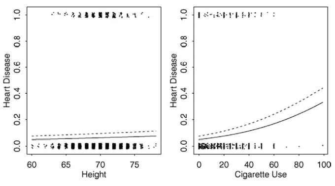
What might affect the chance of getting heart disease? One of the earliest studies addressing this issue started in 1960 and used 3154 healthy men, aged from 39 to 59 , from the San Francisco area. At the start of the study, all were free of heart disease. Eight and a half years later, the study recorded whether these men now suffered from heart disease along with many other variables that might be related to the chance of developing this disease. We load a subset of this data from the Western Collaborative Group Study described in Rosenman et al. (1975): We see that only 257 men developed heart disease as given by the factor variable chd. The men vary in height (in inches) and the number of cigarettes (cigs) smoked per day. We can plot these data using R base graphics:

The first panel in Figure $2.1$ shows a boxplot. This shows the similarity in the distribution of heights of the two groups of men with and without heart disease. But the heart disease is the response variable so we might prefer a plot which treats it as such. We convert the absence/presence of disease into a numerical $0 / 1$ variable and plot this in the second panel of Figure 2.1. Because heights are reported as round numbers of inches and the response can only take two values, it is sensible to add a small amount of noise to each point, called jittering, so that we can distinguish them. Again we can see the similarity in the distributions. We might think about fitting a line to this plot.

More informative plots may be obtained using the ggplot2 package of Wickham (2009). In the first panel of Figure 2.2, we see two histograms showing the distribution of heights for both those with and without heart disease. The dodge option ensures that the two histograms are interleaved. We see that the two similar. We also had to set the bin width of the histogram. It was natural to use one inch as all the height measurements are rounded to the nearest inch. In the second panel of Figure 2.2, we see the corresponding histograms for smoking. In this case, we have shown the frequency rather than the count version of the histogram. We see that smokers are more likely to get heart disease.distributions are

统计代写|广义线性模型代写generalized linear model代考|Logistic Regression

Suppose we have a response variable $Y_i$ for $i=1, \ldots, n$ which takes the values zero or one with $P\left(Y_i=1\right)=p_i$. This response may be related to a set of $q$ predictors $\left(x_{i 1}, \ldots, x_{i q}\right)$. We need a model that describes the relationship of $x_1, \ldots, x_q$ to the probability $p$. Following the linear model approach, we construct a linear predictor:
$$
\eta_i=\beta_0+\beta_1 x_{i 1}+\cdots+\beta_q x_{i q}
$$
Since the linear predictor can accommodate quantitative and qualitative predictors with the use of dummy variables and also allows for transformations and combinations of the original predictors, it is very flexible and yet retains interpretability. The idea that we can express the effect of the predictors on the response solely through the linear predictor is important. The idea can be extended to models for other types of response and is one of the defining features of the wider class of generalized linear models (GLMs) discussed later in Chapter 8.

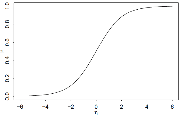
We have seen previously that the linear relation $\eta_i=p_i$ is not workable because we require $0 \leq p_i \leq 1$. Instead we shall use a link function $g$ such that $\eta_i=g\left(p_i\right)$. We need $g$ to be monotone and be such that $0 \leq g^{-1}(\eta) \leq 1$ for any $\eta$. The most popular choice of link function in this situation is the logit. It is defined so that:
$$
\eta=\log (p /(1-p))
$$
or equivalently:
$$
p=\frac{e^\eta}{1+e^\eta}
$$
Combining the use of the logit link with a linear predictor gives us the term logistic regression. Other choices of link function are possible but we will defer discussion of these until later. The logit and its inverse are defined as logit and ilogit in the faraway package. The relationship between $p$ and the linear predictor $\eta$ is shown in Figure 2.4.

广义线性模型代考

统计代写|广义线性模型代写generalized linear model代考|Heart Disease Example

哪些因素会影响患心脏病的几率？解决这个问题的最早研究之一始于 1960 年，使用了来自旧金山地区的 3154 名年龄在 39 至 59 岁之间的健康男性。在研究开始时，所有人都没有心脏病。八年半后，该研究记录了这些人现在是否患有心脏病以及许多其他可能与患这种疾病的机会有关的变量。我们从 Rosenman 等人描述的西方协作组研究中加载该数据的一个子集。(1975)：我们看到只有 257 名男性患上了由因子变量 chd 给出的心脏病。这些人的身高（以英寸为单位）和每天吸的香烟数量各不相同。我们可以使用 R 基础图形绘制这些数据：

第一个面板如图2.1显示箱线图。这表明患有和未患有心脏病的两组男性的身高分布相似。但是心脏病是响应变量，所以我们可能更喜欢这样对待它的情节。我们将疾病的不存在/存在转换为数字0/1变量并将其绘制在图 2.1 的第二个面板中。因为高度以英寸的整数形式报告并且响应只能取两个值，所以向每个点添加少量噪声（称为抖动）是明智的，这样我们就可以区分它们。我们再次可以看到分布的相似性。我们可能会考虑为该图拟合一条线。

使用 Wickham (2009) 的 ggplot2 包可以获得更多信息图。在图 2.2 的第一幅图中，我们看到两个直方图显示了患有和未患有心脏病的人的身高分布。闪避选项确保两个直方图交错。我们看到两者相似。我们还必须设置直方图的 bin 宽度。使用一英寸是很自然的，因为所有的身高测量值都四舍五入到最接近的英寸。在图 2.2 的第二个面板中，我们看到了吸烟的相应直方图。在这种情况下，我们显示的是频率而不是直方图的计数版本。我们看到吸烟者更容易患心脏病。分布是

统计代写|广义线性模型代写generalized linear model代考|Logistic Regression

假设我们有一个响应变量 $Y_i$ 为了 $i=1, \ldots, n$ 它取值零或 $-P\left(Y_i=1\right)=p_i$. 此响应可能与一组 $q$ 预测器 $\left(x_{i 1}, \ldots, x_{i q}\right)$. 我们需要一个描述关系的模型 $x_1, \ldots, x_q$ 概率 $p$. 按照线性模型方法，我们构建了一个线性预测 器:
$$
\eta_i=\beta_0+\beta_1 x_{i 1}+\cdots+\beta_q x_{i q}
$$
由于线性预测器可以通过使用虚拟变量来容纳定量和定性预测器，并且还允许原始预测器的转换和组合，因此它 非常灵活并保留了可解释性。我们可以仅通过线性预测变量来表达预测变量对响应的影响这一想法很重要。这个 想法可以扩展到其他类型响应的模型，并且是第 8 章稍后讨论的更广泛类别的广义线性模型 (GLM) 的定义特征 之一。
我们之前已经看到线性关系 $\eta_i=p_i$ 不可行，因为我们需要 $0 \leq p_i \leq 1$. 相反，我们将使用链接功能 $g$ 这样 $\eta_i=g\left(p_i\right)$. 我们需要 $g$ 是单调的，并且是这样的 $0 \leq g^{-1}(\eta) \leq 1$ 对于任何 $\eta$. 在这种情况下最流行的链接函数 选择是 logit。它被定义为:
$$
\eta=\log (p /(1-p))
$$
或等效地:
$$
p=\frac{e^\eta}{1+e^\eta}
$$
将 logit 链接的使用与线性预测变量相结合，我们就得到了术语逻辑回归。链接功能的其他选择是可能的，但我 们将推迟到以后再讨论这些。logit 及其反函数在 faraway 包中定义为 logit 和 ilogit。之间的关系 $p$ 和线性预测 器 $n$ 如图 $2.4$ 所示。

统计代写请认准statistics-lab™. statistics-lab™为您的留学生涯保驾护航。

金融工程代写

金融工程是使用数学技术来解决金融问题。金融工程使用计算机科学、统计学、经济学和应用数学领域的工具和知识来解决当前的金融问题，以及设计新的和创新的金融产品。

非参数统计代写

非参数统计指的是一种统计方法，其中不假设数据来自于由少数参数决定的规定模型；这种模型的例子包括正态分布模型和线性回归模型。

广义线性模型代考

广义线性模型（GLM）归属统计学领域，是一种应用灵活的线性回归模型。该模型允许因变量的偏差分布有除了正态分布之外的其它分布。

术语 广义线性模型（GLM）通常是指给定连续和/或分类预测因素的连续响应变量的常规线性回归模型。它包括多元线性回归，以及方差分析和方差分析（仅含固定效应）。

有限元方法代写

有限元方法（FEM）是一种流行的方法，用于数值解决工程和数学建模中出现的微分方程。典型的问题领域包括结构分析、传热、流体流动、质量运输和电磁势等传统领域。

有限元是一种通用的数值方法，用于解决两个或三个空间变量的偏微分方程（即一些边界值问题）。为了解决一个问题，有限元将一个大系统细分为更小、更简单的部分，称为有限元。这是通过在空间维度上的特定空间离散化来实现的，它是通过构建对象的网格来实现的：用于求解的数值域，它有有限数量的点。边界值问题的有限元方法表述最终导致一个代数方程组。该方法在域上对未知函数进行逼近。[1] 然后将模拟这些有限元的简单方程组合成一个更大的方程系统，以模拟整个问题。然后，有限元通过变化微积分使相关的误差函数最小化来逼近一个解决方案。

tatistics-lab作为专业的留学生服务机构，多年来已为美国、英国、加拿大、澳洲等留学热门地的学生提供专业的学术服务，包括但不限于Essay代写，Assignment代写，Dissertation代写，Report代写，小组作业代写，Proposal代写，Paper代写，Presentation代写，计算机作业代写，论文修改和润色，网课代做，exam代考等等。写作范围涵盖高中，本科，研究生等海外留学全阶段，辐射金融，经济学，会计学，审计学，管理学等全球99%专业科目。写作团队既有专业英语母语作者，也有海外名校硕博留学生，每位写作老师都拥有过硬的语言能力，专业的学科背景和学术写作经验。我们承诺100%原创，100%专业，100%准时，100%满意。

随机分析代写

随机微积分是数学的一个分支，对随机过程进行操作。它允许为随机过程的积分定义一个关于随机过程的一致的积分理论。这个领域是由日本数学家伊藤清在第二次世界大战期间创建并开始的。

时间序列分析代写

随机过程，是依赖于参数的一组随机变量的全体，参数通常是时间。 随机变量是随机现象的数量表现，其时间序列是一组按照时间发生先后顺序进行排列的数据点序列。通常一组时间序列的时间间隔为一恒定值（如1秒，5分钟，12小时，7天，1年），因此时间序列可以作为离散时间数据进行分析处理。研究时间序列数据的意义在于现实中，往往需要研究某个事物其随时间发展变化的规律。这就需要通过研究该事物过去发展的历史记录，以得到其自身发展的规律。

回归分析代写

多元回归分析渐进（Multiple Regression Analysis Asymptotics）属于计量经济学领域，主要是一种数学上的统计分析方法，可以分析复杂情况下各影响因素的数学关系，在自然科学、社会和经济学等多个领域内应用广泛。

MATLAB代写

MATLAB 是一种用于技术计算的高性能语言。它将计算、可视化和编程集成在一个易于使用的环境中，其中问题和解决方案以熟悉的数学符号表示。典型用途包括：数学和计算算法开发建模、仿真和原型制作数据分析、探索和可视化科学和工程图形应用程序开发，包括图形用户界面构建MATLAB 是一个交互式系统，其基本数据元素是一个不需要维度的数组。这使您可以解决许多技术计算问题，尤其是那些具有矩阵和向量公式的问题，而只需用 C 或 Fortran 等标量非交互式语言编写程序所需的时间的一小部分。MATLAB 名称代表矩阵实验室。MATLAB 最初的编写目的是提供对由 LINPACK 和 EISPACK 项目开发的矩阵软件的轻松访问，这两个项目共同代表了矩阵计算软件的最新技术。MATLAB 经过多年的发展，得到了许多用户的投入。在大学环境中，它是数学、工程和科学入门和高级课程的标准教学工具。在工业领域，MATLAB 是高效研究、开发和分析的首选工具。MATLAB 具有一系列称为工具箱的特定于应用程序的解决方案。对于大多数 MATLAB 用户来说非常重要，工具箱允许您学习和应用专业技术。工具箱是 MATLAB 函数（M 文件）的综合集合，可扩展 MATLAB 环境以解决特定类别的问题。可用工具箱的领域包括信号处理、控制系统、神经网络、模糊逻辑、小波、仿真等。

R语言代写	问卷设计与分析代写
PYTHON代写	回归分析与线性模型代写
MATLAB代写	方差分析与试验设计代写
STATA代写	机器学习/统计学习代写
SPSS代写	计量经济学代写
EVIEWS代写	时间序列分析代写
EXCEL代写	深度学习代写
SQL代写	各种数据建模与可视化代写

如果你也在 怎样代写广义线性模型generalized linear model这个学科遇到相关的难题，请随时右上角联系我们的24/7代写客服。

广义线性模型（GLiM，或GLM）是John Nelder和Robert Wedderburn在1972年制定的一种高级统计建模技术。它是一个包含许多其他模型的总称，它允许响应变量y具有除正态分布以外的误差分布。

statistics-lab™ 为您的留学生涯保驾护航 在代写广义线性模型generalized linear model方面已经树立了自己的口碑, 保证靠谱, 高质且原创的统计Statistics代写服务。我们的专家在代写广义线性模型generalized linear model代写方面经验极为丰富，各种代写广义线性模型generalized linear model相关的作业也就用不着说。

我们提供的广义线性模型generalized linear model及其相关学科的代写，服务范围广, 其中包括但不限于:

• Statistical Inference 统计推断
• Statistical Computing 统计计算
• Advanced Probability Theory 高等概率论
• Advanced Mathematical Statistics 高等数理统计学
• (Generalized) Linear Models 广义线性模型
• Statistical Machine Learning 统计机器学习
• Longitudinal Data Analysis 纵向数据分析
• Foundations of Data Science 数据科学基础

统计代写|广义线性模型代写generalized linear model代考|RANDOM VECTORS

Let the $n \times 1$ random vector $\mathbf{Y}=\left(Y_1, Y_2, \ldots, Y_n\right)^{\prime}$ where $Y_i$ is a random variable for $i=1, \ldots, n$. The vector $\mathbf{Y}$ is a random entity. Therefore, $\mathbf{Y}$ has an expectation; each element of $\mathbf{Y}$ has a variance; and any two elements of $\mathbf{Y}$ have a covariance (assuming the expectations, variances, and covariances exist). The following definitions and theorems describe the structure of random vectors.

Definition 1.3.1 Joint Probability Distribution: The probability distribution of the $n \times 1$ random vector $\mathbf{Y}=\left(Y_1, \ldots, Y_n\right)^{\prime}$ equals the joint probability distribution of $Y_1, \ldots, Y_n$. Denote the distribution of $\mathbf{Y}$ by $f_{\mathbf{Y}}(y)-f_{\mathbf{Y}}\left(y_1, \ldots, y_n\right)$.

Definition 1.3.2 Expectation of a Random Vector: The expected value of the $n \times 1$ random vector $\mathbf{Y}=\left(Y_1, \ldots, Y_n\right)^{\prime}$ is given by $\mathrm{E}(\mathbf{Y})=\left[\mathrm{E}\left(Y_1\right), \ldots, \mathrm{E}\left(Y_n\right)\right]^{\prime}$.
Definition 1.3.3 Covariance Matrix of a Random Vector $\mathbf{Y}$ : The $n \times 1$ random vector $\mathbf{Y}=\left(Y_1, \ldots, Y_n\right)^{\prime}$ has $n \times n$ covariance matrix given by
$$
\operatorname{cov}(\mathbf{Y})=\mathrm{E}\left{[\mathbf{Y}-\mathrm{E}(\mathbf{Y})][\mathbf{Y}-\mathrm{E}(\mathbf{Y})]^{\prime}\right} .
$$
The $i j^{\text {th }}$ element of $\operatorname{cov}(\mathbf{Y})$ equals $\mathrm{E}\left{\left[Y_i-\mathrm{E}\left(Y_i\right)\right]\left[Y_j-\mathrm{E}\left(Y_j\right)\right]\right}$ for $i, j=1, \ldots, n$.
Definition 1.3.4 Linear Transformations of a Random Vector $\mathbf{Y}$ : If $\mathbf{B}$ is an $m \times n$ matrix of constants and $\mathbf{Y}$ is an $n \times 1$ random vector, then the $m \times 1$ random vector BY represents $m$ linear transformations of $\mathbf{Y}$.

The following theorem provides the covariance matrix of linear transformations of a random vector.

Theorem 1.3.1 If $\mathbf{B}$ is an $m \times n$ matrix of constants, $\mathbf{Y}$ is an $n \times 1$ random vector, and $\operatorname{cov}(\mathbf{Y})$ is the $n \times n$ covariance matrix of $\mathbf{Y}$, then the $m \times 1$ random vector $\mathbf{B Y}$ has an $m \times m$ covariance matrix given by $\mathbf{B}[\operatorname{cov}(\mathbf{Y})] \mathbf{B}^{\prime}$.

统计代写|广义线性模型代写generalized linear model代考|MULTIVARIATE NORMAL DISTRIBUTION FUNCTION

Let $Z_1, \ldots, Z_n$ be independent, identically distributed normal random variables with mean 0 and variance 1 . The marginal distribution of $Z_i$ is
$$
f_{Z_i}\left(z_i\right)=(2 \pi)^{-1 / 2} e^{-z_i^2 / 2} \quad-\infty<z_i<\infty
$$
for $i=1, \ldots, n$. Since the $Z_i$ ‘s are independent random variables, the joint probability distribution of the $n \times 1$ random vector $\mathbf{Z}=\left(Z_1, \ldots, Z_n\right)^{\prime}$ is
$$
\begin{aligned}
f_{\mathbf{Z}}(\mathbf{z}) &=(2 \pi)^{-n / 2} e^{-\sum_{i=1}^n z_i^2 / 2} \
&=(2 \pi)^{-n / 2} e^{-\mathbf{z}^{\prime} / 2} \quad-\infty<z_i<\infty
\end{aligned}
$$ for $i=1, \ldots, n$. Let the $n \times 1$ vector $\mathbf{Y}=\mathbf{G Z}+\boldsymbol{\mu}$ where $\mathbf{G}$ is an $n \times n$ nonsingula matrix and $\mu$ is an $n \times 1$ vector. The joint distribution of the $n \times 1$ random vector $\mathbf{Y}$ is
$$
f_{\mathbf{Y}}(\mathbf{y})=|\mathbf{\Sigma}|^{-1 / 2}(2 \pi)^{-n / 2} e^{-\left{(\mathbf{y}-\mu)^{\prime} \mathbf{\Sigma}^{-1}(\mathbf{y}-\mu)\right} / 2} .
$$
where $\boldsymbol{\Sigma}=\mathbf{G G}^{\prime}$ is an $n \times n$ positive definite matrix and the Jacobian for the transformation $\mathbf{Z}=\mathbf{G}^{-1}(\mathbf{Y}-\mu)$ is $\left|\mathbf{G G}^{\prime}\right|^{-1 / 2}=|\mathbf{\Sigma}|^{-1 / 2}$.

The function $f_{\mathbf{Y}}(\mathbf{y})$ is the multivariate normal distribution of an $n \times 1$ random vector $Y$ with $n \times 1$ mean vector $\mu$ and $n \times n$ positive definite covariance matrix $\Sigma$. The following notation will be used to represent this distribution: the $n \times 1$ random vector $\mathbf{Y} \sim \mathrm{N}_n(\mu, \boldsymbol{\Sigma})$.

The moment generating function of an $n$-dimensional multivariate normal random vector is provided in the next theorem.

广义线性模型代考

统计代写|广义线性模型代写generalized linear model代考|RANDOM VECTORS

让 $n \times 1$ 随机向量 $\mathbf{Y}=\left(Y_1, Y_2, \ldots, Y_n\right)^{\prime}$ 在哪里 $Y_i$ 是一个随机变量 $i=1, \ldots, n$. 向量 $\mathbf{Y}$ 是一个随机实体。 所以， $\mathbf{Y}$ 有期望；的每个元素 $\mathbf{Y}$ 有方差；和任意两个元素 $\mathbf{Y}$ 有一个协方差 (假设存在期望、方差和协方差)。 以下定义和定理描述了随机向量的结构。
定义 $1.3 .1$ 联合概率分布: $n \times 1$ 随机向量 $\mathbf{Y}=\left(Y_1, \ldots, Y_n\right)^{\prime}$ 等于联合概率分布 $Y_1, \ldots, Y_n$. 表示分布 $\mathbf{Y}$ 经 过 $f_{\mathbf{Y}}(y)-f_{\mathbf{Y}}\left(y_1, \ldots, y_n\right)$.
定义 1.3.2 随机向量的期望值: $n \times 1$ 随机向量 $\mathbf{Y}=\left(Y_1, \ldots, Y_n\right)^{\prime}$ 是 (谁) 给的 $\mathrm{E}(\mathbf{Y})=\left[\mathrm{E}\left(Y_1\right), \ldots, \mathrm{E}\left(Y_n\right)\right]^{\prime}$
定义 1.3.3 随机向量的协方差矩阵 $\mathbf{Y}:$ 这 $n \times 1$ 随机向量 $\mathbf{Y}=\left(Y_1, \ldots, Y_n\right)^{\prime}$ 有 $n \times n$ 协方差矩阵由下式给出
这 $i j^{\text {th }}$ 的元素 $\operatorname{cov}(\mathbf{Y})$ 等于 $i, j=1, \ldots, n$.
定义 1.3.4 随机向量的线性变换 $\mathbf{Y}:$ : 如果 $\mathbf{B}$ 是一个 $m \times n$ 常数矩阵和 $\mathbf{Y}$ 是一个 $n \times 1$ 随机向量，则 $m \times 1$ 随机 向量 BY 表示 $m$ 的线性变换 $\mathbf{Y}$.
以下定理提供了随机向量的线性变换的协方差矩阵。
定理 $1.3 .1$ 如果 $\mathbf{B}$ 是一个 $m \times n$ 常数矩阵， $\mathbf{Y}$ 是一个 $n \times 1$ 随机向量，和 $\operatorname{cov}(\mathbf{Y})$ 是个 $n \times n$ 的协方差矩阵 $\mathbf{Y}$ ， 那么 $m \times 1$ 随机向量 $\mathbf{B Y}$ 有一个 $m \times m$ 协方差矩阵由下式给出 $\mathbf{B}[\operatorname{cov}(\mathbf{Y})] \mathbf{B}^{\prime}$.

统计代写|广义线性模型代写generalized linear model代考|MULTIVARIATE NORMAL DISTRIBUTION FUNCTION

让 $Z_1, \ldots, Z_n$ 是独立的，同分布的正态随机变量，均值为 0 方差为 1 。边际分布 $Z_i$ 是
$$
f_{Z_i}\left(z_i\right)=(2 \pi)^{-1 / 2} e^{-z_i^2 / 2} \quad-\infty<z_i<\infty
$$
为了 $i=1, \ldots, n$. 由于 $Z_i$ 是独立的随机变量，联合概率分布 $n \times 1$ 随机向量 $\mathbf{Z}=\left(Z_1, \ldots, Z_n\right)^{\prime}$ 是
$$
f_{\mathbf{Z}}(\mathbf{z})=(2 \pi)^{-n / 2} e^{-\sum_{i=1}^n z_i^2 / 2} \quad=(2 \pi)^{-n / 2} e^{-\mathbf{z}^{\prime} / 2} \quad-\infty<z_i<\infty
$$
为了 $i=1, \ldots, n$. 让 $n \times 1$ 向量 $\mathbf{Y}=\mathbf{G Z}+\boldsymbol{\mu}$ 在哪里 $\mathbf{G}$ 是一个 $n \times n$ 非奇异矩阵和 $\mu$ 是一个 $n \times 1$ 向量。联 合分布 $n \times 1$ 随机向量 $\mathbf{Y}$ 是
在哪里 $\boldsymbol{\Sigma}=\mathbf{G G}^{\prime}$ 是一个 $n \times n$ 正定矩阵和用于变㛟的雅可比行列式 $\mathbf{Z}=\mathbf{G}^{-1}(\mathbf{Y}-\mu)$ 是 $\left|\mathbf{G} \mathbf{G}^{\prime}\right|^{-1 / 2}=|\boldsymbol{\Sigma}|^{-1 / 2}$
功能 $f_{\mathbf{Y}}(\mathbf{y})$ 是一个多元正态分布 $n \times 1$ 随机向量 $Y$ 和 $n \times 1$ 平均向量 $\mu$ 和 $n \times n$ 正定协方差矩阵 $\Sigma$. 以下符号将用 于表示此分布: $n \times 1$ 随机向量 $\mathbf{Y} \sim \mathrm{N}_n(\mu, \boldsymbol{\Sigma})$.
的矩生成函数 $n$ 维多元正态随机向量在下一个定理中提供。

统计代写请认准statistics-lab™. statistics-lab™为您的留学生涯保驾护航。

金融工程代写

金融工程是使用数学技术来解决金融问题。金融工程使用计算机科学、统计学、经济学和应用数学领域的工具和知识来解决当前的金融问题，以及设计新的和创新的金融产品。

非参数统计代写

非参数统计指的是一种统计方法，其中不假设数据来自于由少数参数决定的规定模型；这种模型的例子包括正态分布模型和线性回归模型。

广义线性模型代考

广义线性模型（GLM）归属统计学领域，是一种应用灵活的线性回归模型。该模型允许因变量的偏差分布有除了正态分布之外的其它分布。

术语 广义线性模型（GLM）通常是指给定连续和/或分类预测因素的连续响应变量的常规线性回归模型。它包括多元线性回归，以及方差分析和方差分析（仅含固定效应）。

有限元方法代写

有限元方法（FEM）是一种流行的方法，用于数值解决工程和数学建模中出现的微分方程。典型的问题领域包括结构分析、传热、流体流动、质量运输和电磁势等传统领域。

有限元是一种通用的数值方法，用于解决两个或三个空间变量的偏微分方程（即一些边界值问题）。为了解决一个问题，有限元将一个大系统细分为更小、更简单的部分，称为有限元。这是通过在空间维度上的特定空间离散化来实现的，它是通过构建对象的网格来实现的：用于求解的数值域，它有有限数量的点。边界值问题的有限元方法表述最终导致一个代数方程组。该方法在域上对未知函数进行逼近。[1] 然后将模拟这些有限元的简单方程组合成一个更大的方程系统，以模拟整个问题。然后，有限元通过变化微积分使相关的误差函数最小化来逼近一个解决方案。

tatistics-lab作为专业的留学生服务机构，多年来已为美国、英国、加拿大、澳洲等留学热门地的学生提供专业的学术服务，包括但不限于Essay代写，Assignment代写，Dissertation代写，Report代写，小组作业代写，Proposal代写，Paper代写，Presentation代写，计算机作业代写，论文修改和润色，网课代做，exam代考等等。写作范围涵盖高中，本科，研究生等海外留学全阶段，辐射金融，经济学，会计学，审计学，管理学等全球99%专业科目。写作团队既有专业英语母语作者，也有海外名校硕博留学生，每位写作老师都拥有过硬的语言能力，专业的学科背景和学术写作经验。我们承诺100%原创，100%专业，100%准时，100%满意。

随机分析代写

随机微积分是数学的一个分支，对随机过程进行操作。它允许为随机过程的积分定义一个关于随机过程的一致的积分理论。这个领域是由日本数学家伊藤清在第二次世界大战期间创建并开始的。

时间序列分析代写

随机过程，是依赖于参数的一组随机变量的全体，参数通常是时间。 随机变量是随机现象的数量表现，其时间序列是一组按照时间发生先后顺序进行排列的数据点序列。通常一组时间序列的时间间隔为一恒定值（如1秒，5分钟，12小时，7天，1年），因此时间序列可以作为离散时间数据进行分析处理。研究时间序列数据的意义在于现实中，往往需要研究某个事物其随时间发展变化的规律。这就需要通过研究该事物过去发展的历史记录，以得到其自身发展的规律。

回归分析代写

多元回归分析渐进（Multiple Regression Analysis Asymptotics）属于计量经济学领域，主要是一种数学上的统计分析方法，可以分析复杂情况下各影响因素的数学关系，在自然科学、社会和经济学等多个领域内应用广泛。

MATLAB代写

MATLAB 是一种用于技术计算的高性能语言。它将计算、可视化和编程集成在一个易于使用的环境中，其中问题和解决方案以熟悉的数学符号表示。典型用途包括：数学和计算算法开发建模、仿真和原型制作数据分析、探索和可视化科学和工程图形应用程序开发，包括图形用户界面构建MATLAB 是一个交互式系统，其基本数据元素是一个不需要维度的数组。这使您可以解决许多技术计算问题，尤其是那些具有矩阵和向量公式的问题，而只需用 C 或 Fortran 等标量非交互式语言编写程序所需的时间的一小部分。MATLAB 名称代表矩阵实验室。MATLAB 最初的编写目的是提供对由 LINPACK 和 EISPACK 项目开发的矩阵软件的轻松访问，这两个项目共同代表了矩阵计算软件的最新技术。MATLAB 经过多年的发展，得到了许多用户的投入。在大学环境中，它是数学、工程和科学入门和高级课程的标准教学工具。在工业领域，MATLAB 是高效研究、开发和分析的首选工具。MATLAB 具有一系列称为工具箱的特定于应用程序的解决方案。对于大多数 MATLAB 用户来说非常重要，工具箱允许您学习和应用专业技术。工具箱是 MATLAB 函数（M 文件）的综合集合，可扩展 MATLAB 环境以解决特定类别的问题。可用工具箱的领域包括信号处理、控制系统、神经网络、模糊逻辑、小波、仿真等。

R语言代写	问卷设计与分析代写
PYTHON代写	回归分析与线性模型代写
MATLAB代写	方差分析与试验设计代写
STATA代写	机器学习/统计学习代写
SPSS代写	计量经济学代写
EVIEWS代写	时间序列分析代写
EXCEL代写	深度学习代写
SQL代写	各种数据建模与可视化代写

如果你也在 怎样代写广义线性模型generalized linear model这个学科遇到相关的难题，请随时右上角联系我们的24/7代写客服。

广义线性模型（GLiM，或GLM）是John Nelder和Robert Wedderburn在1972年制定的一种高级统计建模技术。它是一个包含许多其他模型的总称，它允许响应变量y具有除正态分布以外的误差分布。

statistics-lab™ 为您的留学生涯保驾护航 在代写广义线性模型generalized linear model方面已经树立了自己的口碑, 保证靠谱, 高质且原创的统计Statistics代写服务。我们的专家在代写广义线性模型generalized linear model代写方面经验极为丰富，各种代写广义线性模型generalized linear model相关的作业也就用不着说。

我们提供的广义线性模型generalized linear model及其相关学科的代写，服务范围广, 其中包括但不限于:

• Statistical Inference 统计推断
• Statistical Computing 统计计算
• Advanced Probability Theory 高等概率论
• Advanced Mathematical Statistics 高等数理统计学
• (Generalized) Linear Models 广义线性模型
• Statistical Machine Learning 统计机器学习
• Longitudinal Data Analysis 纵向数据分析
• Foundations of Data Science 数据科学基础

统计代写|广义线性模型代写generalized linear model代考|Linear Algebra

This representation of a symmetric idempotent matrix is generalized in the next theorem.

Theorem 1.1.10 If $\mathbf{A}$ is an $n \times n$ symmetric, idempotent matrix of rank $r$ then $\mathbf{A}=\mathbf{P P}^{\prime}$ where $\mathbf{P}$ is an $n \times r$ matrix whose columns are the eigenvectors of $\mathbf{A}$ associated with the $r$ eigenvalues equal to 1 .

Proof: Let $\mathbf{A}$ be an $n \times n$ symmetric, idempotent matrix of rank $r$. By Theorem $1.1 .3$
$$
\mathbf{R}^{\prime} \mathbf{A} \mathbf{R}=\left[\begin{array}{cc}
\mathbf{I}_r & \mathbf{0} \
\mathbf{0} & \mathbf{0}
\end{array}\right]
$$
where $\mathbf{R}=[\mathbf{P} \mid \mathbf{Q}]$ is the $n \times n$ matrix of eigenvectors of $\mathbf{A}, \mathbf{P}$ is the $n \times r$ matrix whose $r$ columns are the eigenvectors associated with the $r$ eigenvalues 1 , and $\mathbf{Q}$ is the $n \times(n-r)$ matrix of eigenvectors associated with the $(n-r)$ eigenvalues 0 . Therefore,
$$
\mathbf{A}=\left[\begin{array}{ll}
\mathbf{P} & \mathbf{Q}
\end{array}\right]\left[\begin{array}{cc}
\mathbf{I}_r & 0 \
\mathbf{0} & \mathbf{0}
\end{array}\right]\left[\begin{array}{l}
\mathbf{P}^{\prime} \
\mathbf{Q}^{\prime}
\end{array}\right]=\mathbf{P P}^{\prime} .
$$
Furthermore, $\mathbf{P}^{\prime} \mathbf{P}=\mathbf{I}_r$ because $\mathbf{P}$ is an $n \times r$ matrix of orthogonal eigenvectors.
If $\mathbf{X}^{\prime} \mathbf{A X}$ is a quadratic form with $n \times 1$ vector $\mathbf{X}$ and $n \times n$ symmetric matrix $\mathbf{A}$, then $\mathbf{X}^{\prime} \mathbf{A} \mathbf{X}$ is a quadratic form constructed from an $n$-dimensional vector. The following example uses Theorem $1.1 .10$ to show that if $\mathbf{A}$ is an $n \times n$ symmetric, idempotent matrix of rank $r \leq n$ then the quadratic form $\mathbf{X}^{\prime} \mathbf{A X}$ can be rewritten as a quadratic form constructed from an $r$-dimensional vector.

Example 1.1.14 Let $\mathbf{X}^{\prime} \mathbf{A} \mathbf{X}$ be a quadratic form with $n \times 1$ vector $\mathbf{X}$ and $n \times n$ symmetric, idempotent matrix $\mathbf{A}$ of rank $r \leq n$. By Theorem 1.1.10, $\mathbf{X}^{\prime} \mathbf{A X}=$ $\mathbf{X}^{\prime} \mathbf{P P}^{\prime} \mathbf{X}=\mathbf{Z}^{\prime} \mathbf{Z}$ where $\mathbf{P}$ is an $n \times r$ matrix of eigenvectors of $\mathbf{A}$ associated with the eigenvalues 1 and $\mathbf{Z}=\mathbf{P}^{\prime} \mathbf{X}$ is an $r \times 1$ vector. For a more specific example, note that $\mathbf{X}^{\prime}\left(\mathbf{I}_n-\frac{1}{n} \mathbf{J}_n\right) \mathbf{X}=\mathbf{X}^{\prime} \mathbf{P}_n \mathbf{P}_n^{\prime} \mathbf{X}=\mathbf{Z}^{\prime} \mathbf{Z}$ where $\mathbf{P}_n^{\prime}$ is the $(n-1) \times n$ lower portion of an $n$-dimensional Helmert matrix and $\mathbf{Z}=\mathbf{P}_n^{\prime} \mathbf{X}$ is an $(n-1) \times 1$ vector.

统计代写|广义线性模型代写generalized linear model代考|KRONECKER PRODUCTS

Kronecker products will be used extensively in this text. In this section the Kronecker product operation is defined and a number of related theorems are listed without proof.

Definition 1.2.1 Kronecker Product: If $\mathbf{A}$ is an $r \times s$ matrix with $i j^{\text {th }}$ element $a_{i j}$ for $i=1, \ldots, r$ and $j=1, \ldots, s$, and $\mathbf{B}$ is any $t \times v$ matrix, then the Kronecker product of $\mathbf{A}$ and $\mathbf{B}$, denoted by $\mathbf{A} \otimes \mathbf{B}$, is the $r t \times s v$ matrix formed by multiplying each $a_{i j}$ element by the entire matrix $\mathbf{B}$. That is,
$$
\mathbf{A} \otimes \mathbf{B}=\left[\begin{array}{cccc}
a_{11} \mathbf{B} & a_{12} \mathbf{B} & \cdots & a_{1 s} \mathbf{B} \
a_{21} \mathbf{B} & a_{22} \mathbf{B} & \cdots & a_{2 s} \mathbf{B} \
\vdots & \vdots & \ddots & \vdots \
a_{r 1} \mathbf{B} & a_{r 2} \mathbf{B} & \cdots & a_{r s} \mathbf{B}
\end{array}\right]
$$
Theorem 1.2.1 Let $\mathbf{A}$ and $\mathbf{B}$ be any matrices. Then $(\mathbf{A} \otimes \mathbf{B})^{\prime}=\mathbf{A}^{\prime} \otimes \mathbf{B}^{\prime}$.
Example 1.2.1 $\left[\mathbf{1}_a \otimes(2,1,4)\right]^{\prime}=\mathbf{1}_a^{\prime} \otimes(2,1,4)^{\prime}$.
Theorem 1.2.2 Let $\mathbf{A}, \mathbf{B}$, and $\mathbf{C}$ be any matrices and let $a$ be a scalar. Then $a \mathbf{A} \otimes \mathbf{B} \otimes \mathbf{C}=a(\mathbf{A} \otimes \mathbf{B}) \otimes \mathbf{C}=\mathbf{A} \otimes(a \mathbf{B} \otimes \mathbf{C})$.
Example 1.2.2 $\frac{1}{a} \mathbf{J}_a \otimes \mathbf{J}_b \otimes \mathbf{J}_c=\frac{1}{a}\left[\left(\mathbf{J}_a \otimes \mathbf{J}_b\right) \otimes \mathbf{J}_c\right]=\mathbf{J}_a \otimes\left(\frac{1}{a} \mathbf{J}_b \otimes \mathbf{J}_c\right)$.
Theorem 1.2.3 Let $\mathbf{A}$ and $\mathbf{B}$ be any square matrices. Then $\operatorname{tr}(\mathbf{A} \otimes \mathbf{B})=$ $[\operatorname{tr}(\mathbf{A})][\operatorname{tr}(\mathbf{B})]$

Example 1.2.3 $\operatorname{tr}\left[\left(\mathbf{I}_a-\frac{1}{a} \mathbf{J}_a\right) \otimes\left(\mathbf{I}_n-\frac{1}{n} \mathbf{J}_n\right)\right]=\operatorname{tr}\left[\left(\mathbf{I}_a-\frac{1}{a} \mathbf{J}_a\right)\right] \operatorname{tr}\left[\left(\mathbf{I}_n-\frac{1}{n} \mathbf{J}_n\right)\right]=$ $(a-1)(n-1)$

Theorem 1.2.4 Let $\mathbf{A}$ be an $r \times s$ matrix, $\mathbf{B}$ be a $t \times u$ matrix, $\mathbf{C}$ be an $s \times v$ matrix, and $\mathbf{D}$ be a $u \times w$ matrix. Then $(\mathbf{A} \otimes \mathbf{B})(\mathbf{C} \otimes \mathbf{D})=\mathbf{A C} \otimes \mathbf{B D}$.

广义线性模型代考

统计代写|广义线性模型代写generalized linear model代考|Linear Algebra

对称幂等矩阵的这种表示在下一个定理中得到推广。
定理 1.1.10 如果 $\mathbf{A}$ 是一个 $n \times n$ 对称幂等秩矩阵 $r$ 然后 $\mathbf{A}=\mathbf{P P}^{\prime}$ 在哪里 $\mathbf{P}$ 是一个 $n \times r$ 列是特征向量的矩阵 $\mathbf{A}$ 与 $r$ 特征值等于 1 。
证明: 让A豆 $n \times n$ 对称幕等秩矩阵 $r$. 按定理 $1.1 .3$
在哪里 $\mathbf{R}=[\mathbf{P} \mid \mathbf{Q}]$ 是个 $n \times n$ 的特征向量矩阵 $\mathbf{A}, \mathbf{P}$ 是个 $n \times r$ 矩阵 $r$ 列是与 $r$ 特征值 1 和 $\mathbf{Q}$ 是个 $n \times(n-r)$ 与相关联的特征向量矩阵 $(n-r)$ 特征值 0 。所以，
$$
\mathbf{A}=\left[\begin{array}{ll}
\mathbf{P} & \mathbf{Q}
\end{array}\right]\left[\begin{array}{llll}
\mathbf{I}r & 0 & \mathbf{0} & \mathbf{0} \end{array}\right]\left[\begin{array}{l} \mathbf{P}^{\prime} \ \mathbf{Q}^{\prime} \end{array}\right]=\mathbf{P P}^{\prime} . $$ 此外， $\mathbf{P}^{\prime} \mathbf{P}=\mathbf{I}_r$ 因为 $\mathbf{P}$ 是一个 $n \times r$ 正交特征向量矩阵。 如果 $\mathbf{X}^{\prime} \mathbf{A X}$ 是一个二次形式 $n \times 1$ 向量 $\mathbf{X}$ 和 $n \times n$ 对称矩阵 $\mathbf{A}$ ，然后 $\mathbf{X}^{\prime} \mathbf{A} \mathbf{X}$ 是一个二次形式，由 $n$ 维向量。 以下示例使用定理1.1.10证明如果 $\mathbf{A}$ 是一个 $n \times n$ 对称幂等秩矩阵 $r \leq n$ 然后是二次形式 $\mathbf{X}^{\prime} \mathbf{A} \mathbf{X}$ 可以重写为由 $r$ 维向量。 示例 1.1.14 让 $\mathbf{X}^{\prime} \mathbf{A} \mathbf{X}$ 是一个二次形式 $n \times 1$ 向量 $\mathbf{X}$ 和 $n \times n$ 对称的幂等矩阵 $\mathbf{A}$ 等级 $r \leq n$. 根据定理 1.1.10， $\mathbf{X}^{\prime} \mathbf{A} \mathbf{X}=\mathbf{X}^{\prime} \mathbf{P P}^{\prime} \mathbf{X}=\mathbf{Z}^{\prime} \mathbf{Z}$ 在哪里 $\mathbf{P}$ 是一个 $n \times r$ 的特征向量矩阵 $\mathbf{A}$ 与特征值 1 和 $\mathbf{Z}=\mathbf{P}^{\prime} \mathbf{X}{\text {是一个 }} \times 1$ 向量。对于更具体的示例，请注意 $\mathbf{X}^{\prime}\left(\mathbf{I}_n-\frac{1}{n} \mathbf{J}_n\right) \mathbf{X}=\mathbf{X}^{\prime} \mathbf{P}_n \mathbf{P}_n^{\prime} \mathbf{X}=\mathbf{Z}^{\prime} \mathbf{Z}$ 在哪里 $\mathbf{P}_n^{\prime}$ 是个 $(n-1) \times n$ 的 下部 $n$ 维 Helmert 矩阵和 $\mathbf{Z}=\mathbf{P}_n^{\prime} \mathbf{X}$ 是一个 $(n-1) \times 1$ 向量。

统计代写|广义线性模型代写generalized linear model代考|KRONECKER PRODUCTS

Kronecker 产品将在本文中广泛使用。在本节中，定义了克罗内克乘积运算，并列出了许多相关的定理，但没有 证明。
定义 1.2.1 克罗内克积: 如果 $\mathbf{A}$ 是一个 $r \times s$ 矩阵与 $i j^{\text {th }}$ 元素 $a_{i j}$ 为了i $i, \ldots, r$ 和 $j=1, \ldots, s$ ，和 $\mathbf{B}$ 是任 何 $t \times v$ 矩阵，然后是克罗内克积 $\mathbf{A}$ 和 $\mathbf{B}$ ，表示为 $\mathbf{A} \otimes \mathbf{B}$ ，是个 $r t \times s v$ 每个相乘形成的矩阵 $a_{i j}$ 整个矩阵的元 素 $\mathbf{B}$. 那是，
定理 1.2.1 令 $\mathbf{A}$ 和 $\mathbf{B}$ 是任何矩阵。然后 $(\mathbf{A} \otimes \mathbf{B})^{\prime}=\mathbf{A}^{\prime} \otimes \mathbf{B}^{\prime}$.
示例 1.2.1 $\left[\mathbf{1}_a \otimes(2,1,4)\right]^{\prime}=\mathbf{1}_a^{\prime} \otimes(2,1,4)^{\prime}$.
定理 1.2.2 让 $\mathbf{A}, \mathbf{B}$ ，和 $\mathbf{C}$ 是任何矩阵并让 $a$ 是一个标量。然后
$a \mathbf{A} \otimes \mathbf{B} \otimes \mathbf{C}=a(\mathbf{A} \otimes \mathbf{B}) \otimes \mathbf{C}=\mathbf{A} \otimes(a \mathbf{B} \otimes \mathbf{C})$.
示例 1.2.2 $\frac{1}{a} \mathbf{J}_a \otimes \mathbf{J}_b \otimes \mathbf{J}_c=\frac{1}{a}\left[\left(\mathbf{J}_a \otimes \mathbf{J}_b\right) \otimes \mathbf{J}_c\right]=\mathbf{J}_a \otimes\left(\frac{1}{a} \mathbf{J}_b \otimes \mathbf{J}_c\right)$.
定理 1.2.3 让 $\mathbf{A}$ 和 $\mathbf{B}$ 是任何方阵。然后 $\operatorname{tr}(\mathbf{A} \otimes \mathbf{B})=[\operatorname{tr}(\mathbf{A})][\operatorname{tr}(\mathbf{B})]$
示例 1.2.3tr $\left[\left(\mathbf{I}_a-\frac{1}{a} \mathbf{J}_a\right) \otimes\left(\mathbf{I}_n-\frac{1}{n} \mathbf{J}_n\right)\right]=\operatorname{tr}\left[\left(\mathbf{I}_a-\frac{1}{a} \mathbf{J}_a\right)\right] \operatorname{tr}\left[\left(\mathbf{I}_n-\frac{1}{n} \mathbf{J}_n\right)\right]=(a-1)(n-1)$
定理 1.2.4 让 $\mathbf{A}$ 豆 $r \times s$ 矩阵， $\mathbf{B}$ 做一个 $t \times u$ 矩阵， $\mathbf{C}$ 豆 $s \times v$ 矩阵，和 $\mathbf{D}$ 做一个 $u \times w$ 矩阵。然后 $(\mathbf{A} \otimes \mathbf{B})(\mathbf{C} \otimes \mathbf{D})=\mathbf{A} \mathbf{C} \otimes \mathbf{B D}$.

统计代写请认准statistics-lab™. statistics-lab™为您的留学生涯保驾护航。

金融工程代写

金融工程是使用数学技术来解决金融问题。金融工程使用计算机科学、统计学、经济学和应用数学领域的工具和知识来解决当前的金融问题，以及设计新的和创新的金融产品。

非参数统计代写

非参数统计指的是一种统计方法，其中不假设数据来自于由少数参数决定的规定模型；这种模型的例子包括正态分布模型和线性回归模型。

广义线性模型代考

广义线性模型（GLM）归属统计学领域，是一种应用灵活的线性回归模型。该模型允许因变量的偏差分布有除了正态分布之外的其它分布。

术语 广义线性模型（GLM）通常是指给定连续和/或分类预测因素的连续响应变量的常规线性回归模型。它包括多元线性回归，以及方差分析和方差分析（仅含固定效应）。

有限元方法代写

有限元方法（FEM）是一种流行的方法，用于数值解决工程和数学建模中出现的微分方程。典型的问题领域包括结构分析、传热、流体流动、质量运输和电磁势等传统领域。

有限元是一种通用的数值方法，用于解决两个或三个空间变量的偏微分方程（即一些边界值问题）。为了解决一个问题，有限元将一个大系统细分为更小、更简单的部分，称为有限元。这是通过在空间维度上的特定空间离散化来实现的，它是通过构建对象的网格来实现的：用于求解的数值域，它有有限数量的点。边界值问题的有限元方法表述最终导致一个代数方程组。该方法在域上对未知函数进行逼近。[1] 然后将模拟这些有限元的简单方程组合成一个更大的方程系统，以模拟整个问题。然后，有限元通过变化微积分使相关的误差函数最小化来逼近一个解决方案。

tatistics-lab作为专业的留学生服务机构，多年来已为美国、英国、加拿大、澳洲等留学热门地的学生提供专业的学术服务，包括但不限于Essay代写，Assignment代写，Dissertation代写，Report代写，小组作业代写，Proposal代写，Paper代写，Presentation代写，计算机作业代写，论文修改和润色，网课代做，exam代考等等。写作范围涵盖高中，本科，研究生等海外留学全阶段，辐射金融，经济学，会计学，审计学，管理学等全球99%专业科目。写作团队既有专业英语母语作者，也有海外名校硕博留学生，每位写作老师都拥有过硬的语言能力，专业的学科背景和学术写作经验。我们承诺100%原创，100%专业，100%准时，100%满意。

随机分析代写

随机微积分是数学的一个分支，对随机过程进行操作。它允许为随机过程的积分定义一个关于随机过程的一致的积分理论。这个领域是由日本数学家伊藤清在第二次世界大战期间创建并开始的。

时间序列分析代写

随机过程，是依赖于参数的一组随机变量的全体，参数通常是时间。 随机变量是随机现象的数量表现，其时间序列是一组按照时间发生先后顺序进行排列的数据点序列。通常一组时间序列的时间间隔为一恒定值（如1秒，5分钟，12小时，7天，1年），因此时间序列可以作为离散时间数据进行分析处理。研究时间序列数据的意义在于现实中，往往需要研究某个事物其随时间发展变化的规律。这就需要通过研究该事物过去发展的历史记录，以得到其自身发展的规律。

回归分析代写

多元回归分析渐进（Multiple Regression Analysis Asymptotics）属于计量经济学领域，主要是一种数学上的统计分析方法，可以分析复杂情况下各影响因素的数学关系，在自然科学、社会和经济学等多个领域内应用广泛。

MATLAB代写

MATLAB 是一种用于技术计算的高性能语言。它将计算、可视化和编程集成在一个易于使用的环境中，其中问题和解决方案以熟悉的数学符号表示。典型用途包括：数学和计算算法开发建模、仿真和原型制作数据分析、探索和可视化科学和工程图形应用程序开发，包括图形用户界面构建MATLAB 是一个交互式系统，其基本数据元素是一个不需要维度的数组。这使您可以解决许多技术计算问题，尤其是那些具有矩阵和向量公式的问题，而只需用 C 或 Fortran 等标量非交互式语言编写程序所需的时间的一小部分。MATLAB 名称代表矩阵实验室。MATLAB 最初的编写目的是提供对由 LINPACK 和 EISPACK 项目开发的矩阵软件的轻松访问，这两个项目共同代表了矩阵计算软件的最新技术。MATLAB 经过多年的发展，得到了许多用户的投入。在大学环境中，它是数学、工程和科学入门和高级课程的标准教学工具。在工业领域，MATLAB 是高效研究、开发和分析的首选工具。MATLAB 具有一系列称为工具箱的特定于应用程序的解决方案。对于大多数 MATLAB 用户来说非常重要，工具箱允许您学习和应用专业技术。工具箱是 MATLAB 函数（M 文件）的综合集合，可扩展 MATLAB 环境以解决特定类别的问题。可用工具箱的领域包括信号处理、控制系统、神经网络、模糊逻辑、小波、仿真等。

R语言代写	问卷设计与分析代写
PYTHON代写	回归分析与线性模型代写
MATLAB代写	方差分析与试验设计代写
STATA代写	机器学习/统计学习代写
SPSS代写	计量经济学代写
EVIEWS代写	时间序列分析代写
EXCEL代写	深度学习代写
SQL代写	各种数据建模与可视化代写

如果你也在 怎样代写广义线性模型generalized linear model这个学科遇到相关的难题，请随时右上角联系我们的24/7代写客服。

广义线性模型（GLiM，或GLM）是John Nelder和Robert Wedderburn在1972年制定的一种高级统计建模技术。它是一个包含许多其他模型的总称，它允许响应变量y具有除正态分布以外的误差分布。

statistics-lab™ 为您的留学生涯保驾护航 在代写广义线性模型generalized linear model方面已经树立了自己的口碑, 保证靠谱, 高质且原创的统计Statistics代写服务。我们的专家在代写广义线性模型generalized linear model代写方面经验极为丰富，各种代写广义线性模型generalized linear model相关的作业也就用不着说。

我们提供的广义线性模型generalized linear model及其相关学科的代写，服务范围广, 其中包括但不限于:

• Statistical Inference 统计推断
• Statistical Computing 统计计算
• Advanced Probability Theory 高等概率论
• Advanced Mathematical Statistics 高等数理统计学
• (Generalized) Linear Models 广义线性模型
• Statistical Machine Learning 统计机器学习
• Longitudinal Data Analysis 纵向数据分析
• Foundations of Data Science 数据科学基础

统计代写|广义线性模型代写generalized linear model代考|ELEMENTARY MATRIX CONCEPTS

The following list of definitions provides a brief summary of some useful matrix operations.

Definition 1.1.1 Matrix: An $r \times s$ matrix $\mathbf{A}$ is a rectangular array of elements with $r$ rows and $s$ columns. An $r \times 1$ vector $\mathbf{Y}$ is a matrix with $r$ rows and 1 column. Matrix elements are restricted to real numbers throughout the text.

Definition 1.1.2 Transpose: If $\mathbf{A}$ is an $n \times s$ matrix, then the transpose of $\mathbf{A}$, denoted by $\mathbf{A}^{\prime}$, is an $s \times n$ matrix formed by interchanging the rows and columns of $\mathbf{A}$.

Definition 1.1.3 Identity Matrix, Matrix of Ones and Zeros: $\mathbf{I}n$ represents an $n \times n$ identity matrix, $\mathbf{J}_n$ is an $n \times n$ matrix of ones, $\mathbf{1}_n$ is an $n \times 1$ vector of ones, and $\mathbf{0}{m \times n}$ is an $m \times n$ matrix of zeros.

Definition 1.1.4 Multiplication of Matrices: Let $a_{i j}$ represent the $i j^{\text {th }}$ element of an $r \times s$ matrix $\mathbf{A}$ with $i=1, \ldots, r$ rows and $j=1, \ldots, s$ columns. Likewise, let $b_{j k}$ represent the $j k^{\text {th }}$ element of an $s \times t$ matrix $\mathbf{B}$ with $j=1, \ldots, s$ rows and $k=1, \ldots, t$ columns. The matrix multiplication of $\mathbf{A}$ and $\mathbf{B}$ is represented by $\mathbf{A B}=\mathbf{C}$ where $\mathbf{C}$ is an $r \times t$ matrix whose $i k^{\text {th }}$ element $c_{i k}=\sum_{j=1}^s a_{i j} b_{j k}$. If the $r \times s$ matrix $\mathbf{A}$ is multiplied by a scalar $d$, then the resulting $r \times s$ matrix $d \mathbf{A}$ has $i j^{\text {th }}$ element $d a_{i j}$.
Example 1.1.1 The following matrix multiplications commonly occur.
$$
\begin{aligned}
\mathbf{1}n^{\prime} \mathbf{1}_n &=n \ \mathbf{1}_n \mathbf{1}_n^{\prime} &=\mathbf{J}_n \ \mathbf{J}_n \mathbf{J}_n &=n \mathbf{J}_n \ \mathbf{1}_n^{\prime}\left(\mathbf{I}_n-\frac{1}{n} \mathbf{J}_n\right) &=\mathbf{0}{1 \times n} \
\mathbf{J}n^{\prime}\left(\mathbf{I}_n-\frac{1}{n} \mathbf{J}_n\right) &=\mathbf{0}{n \times n} \
\left(\mathbf{I}n-\frac{1}{n} \mathbf{J}_n\right)\left(\mathbf{I}_n-\frac{1}{n} \mathbf{J}_n\right) &=\left(\mathbf{I}_n-\frac{1}{n} \mathbf{J}_n\right) . \end{aligned} $$ Definition 1.1.5 Addition of Matrices: The sum of two $r \times s$ matrices $\mathbf{A}$ and $\mathbf{B}$ is represented by $\mathbf{A}+\mathbf{B}=\mathbf{C}$ where $\mathbf{C}$ is the $r \times s$ matrix whose $i j^{\text {th }}$ element $c{i j}=a_{i j}+b_{i j}$

统计代写|广义线性模型代写generalized linear model代考|Linear Algebra

It is assumed that the reader is familiar with the definition of the determinant of a square matrix. Therefore, a rigorous definition is omitted. The next definition actually provides the notation used for a determinant.

Definition 1.1.10 Determinant of a Square Matrix: Let $\operatorname{det}(\mathbf{A})=|\mathbf{A}|$ denote the determinant of an $n \times n$ matrix $\mathbf{A}$. Note $\operatorname{det}(\mathbf{A})=0$ if $\mathbf{A}$ is singular.

Definition 1.1.11 Symmetric Matrix: An $n \times n$ matrix $\mathbf{A}$ is symmetric if $\mathbf{A}=\mathbf{A}^{\prime}$.
Definition 1.1.12 Linear Dependence and the Rank of a Matrix: Let A be an $n \times s$ matrix $(s \leq n)$ where $\mathbf{a}_1, \ldots, \mathbf{a}_s$ represent the $s n \times 1$ column vectors of $\mathbf{A}$. The $s$ vectors $\mathbf{a}_1, \ldots, \mathbf{a}_s$ are linearly dependent provided there exists $s$ elements $k_1, \ldots, k_s$, not all zero, such that $k_1 \mathbf{a}_1+\cdots+k_s \mathbf{a}_s=0$. Otherwise, the $s$ vectors are linearly independent. Furthermore, if there are exactly $r \leq s$ vectors of the set $\mathbf{a}_1, \ldots, \mathbf{a}_s$ which are linearly independent, while the remaining $s-r$ can be expressed as a linear combination of these $r$ vectors, then the rank of $\mathbf{A}$, denoted by rank (A), is $r$.

The following list shows the results of the preceding definitions and are stated without proof:
Result 1.1: Let $\mathbf{A}$ and $\mathbf{B}$ each be $n \times n$ nonsingular matrices. Then $(\mathbf{A B})^{-1}=\mathbf{B}^{-1} \mathbf{A}^{-1}$.
Result 1.2: Let $\mathbf{A}$ and $\mathbf{B}$ be any two matrices such that $\mathbf{A B}$ is defined. Then $(\mathbf{A B})^{\prime}=\mathbf{B}^{\prime} \mathbf{A}^{\prime}$.
Result 1.3: Let $\mathbf{A}$ be any matrix. The $\mathbf{A}^{\prime} \mathbf{A}$ and $\mathbf{A} \mathbf{A}^{\prime}$ are symmetric.
Result 1.4: Let $\mathbf{A}$ and $\mathbf{B}$ each be $n \times n$ matrices. Then $\operatorname{det}(\mathbf{A B})=$ [det(A)][det(B)].
Result 1.5: Let $\mathbf{A}$ and $\mathbf{B}$ be $m \times n$ and $n \times m$ matrices, respectively. Then $\operatorname{tr}(\mathbf{A B})=\operatorname{tr}(\mathbf{B A})$

广义线性模型代考

统计代写|广义线性模型代写generalized linear model代考|ELEMENTARY MATRIX CONCEPTS

下面的定义列表提供了一些有用的矩阵运算的简要总结。
定义 1.1.1 矩阵: 一个 $r \times s$ 矩阵 $\mathbf{A}$ 是一个矩形的元素数组 $r$ 行和 $s$ 列。一个 $r \times 1$ 向量 $\mathbf{Y}$ 是一个矩阵 $r$ 行和 1 列。 整篇文章中，矩阵元素仅限于实数。
定义 1.1.2 转置: 如果 $\mathbf{A}$ 是一个 $n \times s$ 矩阵，然后转置 $\mathbf{A}$ ，表示为 $\mathbf{A}^{\prime}$ ，是一个 $s \times n$ 矩阵的行和列互换形成的 矩阵 $\mathbf{A}$.
定义 $1.1 .3$ 单位矩阵， 1 和 0 矩阵: $\mathbf{I} n$ 代表一个 $n \times n$ 单位矩阵， $\mathbf{J}n$ 是一个 $n \times n$ 的矩阵， $\mathbf{1}_n$ 是一个 $n \times 1$ 个 向量，和 $\mathbf{0} m \times n$ 是一个 $m \times n$ 零矩阵。 定义 $1.1 .4$ 矩阵乘法: 让 $a{i j}$ 代表 $i j^{\text {th }}$ 一个元素 $r \times s$ 矩阵 $\mathbf{A}$ 和 $i=1, \ldots, r$ 行和 $j=1, \ldots, s$ 列。同样，让 $b_{j k}$ 代表 $j k^{\text {th }}$ 一个元素 $s \times t$ 矩阵 $\mathbf{B}$ 和 $j=1, \ldots, s$ 行和 $k=1, \ldots, t$ 列。的矩阵乘法 $\mathbf{A}$ 和 $\mathbf{B}$ 表示为 $\mathbf{A B}=\mathbf{C}$ 在 哪里 $\mathbf{C}$ 是一个 $r \times t$ 矩阵 $i k^{\text {th }}$ 元素 $c_{i k}=\sum_{j=1}^s a_{i j} b_{j k}$. 如果 $r \times s$ 矩阵 $\mathbf{A}$ 乘以一个标量 $d$ 那么结果 $r \times s$ 矩阵 $d \mathbf{A}$ 有 $i j^{\text {th }}$ 元素 $d a_{i j}$.
示例 $1.1 .1$ 通常会出现以下矩阵乘法。
$$
\mathbf{1}^{\prime} \mathbf{1}n=n \mathbf{1}_n \mathbf{1}_n^{\prime} \quad=\mathbf{J}_n \mathbf{J}_n \mathbf{J}_n=n \mathbf{J}_n \mathbf{1}_n^{\prime}\left(\mathbf{I}_n-\frac{1}{n} \mathbf{J}_n\right) \quad=\mathbf{0} 1 \times n \mathbf{J} n^{\prime}\left(\mathbf{I}_n-\frac{1}{n} \mathbf{J}_n\right)=\mathbf{0} n \times n $$ 定义 1.1.5 矩阵相加: 两个之和 $r \times s$ 矩阵 $\mathbf{A}$ 和 $\mathbf{B}$ 表示为 $\mathbf{A}+\mathbf{B}=\mathbf{C}$ 在哪里 $\mathbf{C}$ 是个 $r \times s s^{\text {矩阵 } i j^{\text {th }}}$ 元素 $c i j=a{i j}+b_{i j}$

统计代写|广义线性模型代写generalized linear model代考|Linear Algebra

假设读者熟乎方阵行列式的定义。因此，省略了严格的定义。下一个定义实际上提供了用于行列式的符号。
定义 1.1.10 方阵的行列式: 让 $\operatorname{det}(\mathbf{A})=|\mathbf{A}|$ 表示一个的行列式 $n \times n$ 矩阵 $\mathbf{A}$. 笔记det $(\mathbf{A})=0$ 如果 $\mathbf{A}$ 是单 数。
定义 1.1.11 对称矩阵: 一个 $n \times n$ 矩阵 $\mathbf{A}$ 是对称的，如果 $\mathbf{A}=\mathbf{A}^{\prime}$.
定义 1.1.12 线性相关和矩阵的秩: 设 A 为 $n \times s$ 矩阵 $(s \leq n)$ 在哪里 $\mathbf{a}_1, \ldots, \mathbf{a}_s$ 代表 $s n \times 1$ 的列向量 $\mathbf{A}$. 这 $s$ 矢量图 $\mathbf{a}_1, \ldots, \mathbf{a}_s$ 如果存在，则线性相关 $s$ 元素 $k_1, \ldots, k_s$ ，并非全为零，这样 $k_1 \mathbf{a}_1+\cdots+k_s \mathbf{a}_s=0$. 否 则，该 $s$ 向量是线性无关的。此外，如果有确切的 $r \leq s$ 集合的向量 $\mathbf{a}_1, \ldots, \mathbf{a}_s$ 它们是线性独立的，而其余的 $s-r$ 可以表示为这些的线性组合 $r$ 向量，然后的秩 $\mathbf{A}$ ，用等级 (A) 表示，是 $r$.
下面的列表显示了前面定义的结果，并且没有证明:
结果 1.1：让 $\mathbf{A}$ 和 $\mathbf{B}$ 每个都是 $n \times n$ 非奇异矩阵。然后 $(\mathbf{A B})^{-1}=\mathbf{B}^{-1} \mathbf{A}^{-1}$.
结果 1.2：让 $\mathbf{A}$ 和 $\mathbf{B}$ 是任意两个矩阵，使得 $\mathbf{A} \mathbf{B}$ 被定义为。然后 $(\mathbf{A B})^{\prime}=\mathbf{B}^{\prime} \mathbf{A}^{\prime}$.
结果 1.3: 让 $\mathbf{A}$ 是任何矩阵。这 $\mathbf{A}^{\prime} \mathbf{A}$ 和 $\mathbf{A} \mathbf{A}^{\prime}$ 是对称的。
结果 1.4：让 $\mathbf{A}$ 和 $\mathbf{B}$ 每个都是 $n \times n$ 矩阵。然后 $\operatorname{det}(\mathbf{A B})=[$ 它(A)] $[$ 它(B)]。
结果 1.5：容易 $\mathbf{A}$ 和 $\mathbf{B}$ 是 $m \times n$ 和 $n \times m$ 矩阵，分别。然后 $\operatorname{tr}(\mathbf{A B})=\operatorname{tr}(\mathbf{B} \mathbf{A})$

统计代写请认准statistics-lab™. statistics-lab™为您的留学生涯保驾护航。

金融工程代写

金融工程是使用数学技术来解决金融问题。金融工程使用计算机科学、统计学、经济学和应用数学领域的工具和知识来解决当前的金融问题，以及设计新的和创新的金融产品。

非参数统计代写

非参数统计指的是一种统计方法，其中不假设数据来自于由少数参数决定的规定模型；这种模型的例子包括正态分布模型和线性回归模型。

广义线性模型代考

广义线性模型（GLM）归属统计学领域，是一种应用灵活的线性回归模型。该模型允许因变量的偏差分布有除了正态分布之外的其它分布。

术语 广义线性模型（GLM）通常是指给定连续和/或分类预测因素的连续响应变量的常规线性回归模型。它包括多元线性回归，以及方差分析和方差分析（仅含固定效应）。

有限元方法代写

有限元方法（FEM）是一种流行的方法，用于数值解决工程和数学建模中出现的微分方程。典型的问题领域包括结构分析、传热、流体流动、质量运输和电磁势等传统领域。

有限元是一种通用的数值方法，用于解决两个或三个空间变量的偏微分方程（即一些边界值问题）。为了解决一个问题，有限元将一个大系统细分为更小、更简单的部分，称为有限元。这是通过在空间维度上的特定空间离散化来实现的，它是通过构建对象的网格来实现的：用于求解的数值域，它有有限数量的点。边界值问题的有限元方法表述最终导致一个代数方程组。该方法在域上对未知函数进行逼近。[1] 然后将模拟这些有限元的简单方程组合成一个更大的方程系统，以模拟整个问题。然后，有限元通过变化微积分使相关的误差函数最小化来逼近一个解决方案。

tatistics-lab作为专业的留学生服务机构，多年来已为美国、英国、加拿大、澳洲等留学热门地的学生提供专业的学术服务，包括但不限于Essay代写，Assignment代写，Dissertation代写，Report代写，小组作业代写，Proposal代写，Paper代写，Presentation代写，计算机作业代写，论文修改和润色，网课代做，exam代考等等。写作范围涵盖高中，本科，研究生等海外留学全阶段，辐射金融，经济学，会计学，审计学，管理学等全球99%专业科目。写作团队既有专业英语母语作者，也有海外名校硕博留学生，每位写作老师都拥有过硬的语言能力，专业的学科背景和学术写作经验。我们承诺100%原创，100%专业，100%准时，100%满意。

随机分析代写

随机微积分是数学的一个分支，对随机过程进行操作。它允许为随机过程的积分定义一个关于随机过程的一致的积分理论。这个领域是由日本数学家伊藤清在第二次世界大战期间创建并开始的。

时间序列分析代写

随机过程，是依赖于参数的一组随机变量的全体，参数通常是时间。 随机变量是随机现象的数量表现，其时间序列是一组按照时间发生先后顺序进行排列的数据点序列。通常一组时间序列的时间间隔为一恒定值（如1秒，5分钟，12小时，7天，1年），因此时间序列可以作为离散时间数据进行分析处理。研究时间序列数据的意义在于现实中，往往需要研究某个事物其随时间发展变化的规律。这就需要通过研究该事物过去发展的历史记录，以得到其自身发展的规律。

回归分析代写

多元回归分析渐进（Multiple Regression Analysis Asymptotics）属于计量经济学领域，主要是一种数学上的统计分析方法，可以分析复杂情况下各影响因素的数学关系，在自然科学、社会和经济学等多个领域内应用广泛。

MATLAB代写

MATLAB 是一种用于技术计算的高性能语言。它将计算、可视化和编程集成在一个易于使用的环境中，其中问题和解决方案以熟悉的数学符号表示。典型用途包括：数学和计算算法开发建模、仿真和原型制作数据分析、探索和可视化科学和工程图形应用程序开发，包括图形用户界面构建MATLAB 是一个交互式系统，其基本数据元素是一个不需要维度的数组。这使您可以解决许多技术计算问题，尤其是那些具有矩阵和向量公式的问题，而只需用 C 或 Fortran 等标量非交互式语言编写程序所需的时间的一小部分。MATLAB 名称代表矩阵实验室。MATLAB 最初的编写目的是提供对由 LINPACK 和 EISPACK 项目开发的矩阵软件的轻松访问，这两个项目共同代表了矩阵计算软件的最新技术。MATLAB 经过多年的发展，得到了许多用户的投入。在大学环境中，它是数学、工程和科学入门和高级课程的标准教学工具。在工业领域，MATLAB 是高效研究、开发和分析的首选工具。MATLAB 具有一系列称为工具箱的特定于应用程序的解决方案。对于大多数 MATLAB 用户来说非常重要，工具箱允许您学习和应用专业技术。工具箱是 MATLAB 函数（M 文件）的综合集合，可扩展 MATLAB 环境以解决特定类别的问题。可用工具箱的领域包括信号处理、控制系统、神经网络、模糊逻辑、小波、仿真等。

R语言代写	问卷设计与分析代写
PYTHON代写	回归分析与线性模型代写
MATLAB代写	方差分析与试验设计代写
STATA代写	机器学习/统计学习代写
SPSS代写	计量经济学代写
EVIEWS代写	时间序列分析代写
EXCEL代写	深度学习代写
SQL代写	各种数据建模与可视化代写

如果你也在 怎样代写广义线性模型generalized linear model这个学科遇到相关的难题，请随时右上角联系我们的24/7代写客服。

广义线性模型（GLiM，或GLM）是John Nelder和Robert Wedderburn在1972年制定的一种高级统计建模技术。它是一个包含许多其他模型的总称，它允许响应变量y具有除正态分布以外的误差分布。

statistics-lab™ 为您的留学生涯保驾护航 在代写广义线性模型generalized linear model方面已经树立了自己的口碑, 保证靠谱, 高质且原创的统计Statistics代写服务。我们的专家在代写广义线性模型generalized linear model代写方面经验极为丰富，各种代写广义线性模型generalized linear model相关的作业也就用不着说。

我们提供的广义线性模型generalized linear model及其相关学科的代写，服务范围广, 其中包括但不限于:

• Statistical Inference 统计推断
• Statistical Computing 统计计算
• Advanced Probability Theory 高等概率论
• Advanced Mathematical Statistics 高等数理统计学
• (Generalized) Linear Models 广义线性模型
• Statistical Machine Learning 统计机器学习
• Longitudinal Data Analysis 纵向数据分析
• Foundations of Data Science 数据科学基础

统计代写|广义线性模型代写generalized linear model代考|Multivariate Normal Distribution

In the following examples mean vectors and covariance matrices are derived for a few common problems.

Example 2.1.3 Let $Y_1, \ldots, Y_n$ be independent, identically distributed $\mathrm{N}_1\left(\alpha, \sigma^2\right)$ random variables. By Theorem 2.1.4 $\operatorname{cov}\left(Y_i, Y_j\right)=0$ for $i \neq j$. Furthermore, $\mathrm{E}\left(Y_i\right)=\alpha$ and the $\operatorname{var}\left(Y_i\right)=\sigma^2$ for all $i=1, \ldots, n$. Therefore, the $n \times 1$ random vector $\mathbf{Y}=\left(Y_1, \ldots, Y_n\right)^{\prime} \sim \mathrm{N}_n\left(\alpha \mathbf{1}_n, \sigma^2 \mathbf{I}_n\right)$.

Example 2.1.4 Consider the one-way classification described in Example 1.2.10. Let $Y_{i j}$ be a random variable representing the $j^{\text {th }}$ replicate observation in the $i^{\text {th }}$ level of the fixed factor for $i=1, \ldots, t$ and $j=1, \ldots, r$. Let the $\operatorname{tr} \times 1$ random vector $\left.\mathbf{Y}=Y_{11}, \ldots, Y_{1 r}, \ldots, Y_{t 1}, \ldots, Y_{t r}\right)^{\prime}$ where the $Y_{i j}$ ‘s are assumed to be independent, normally distributed random variables with $\mathrm{E}\left(Y_{i j}\right)=\mu_i$ and $\operatorname{var}\left(Y_{i j}\right)=\sigma^2$. This experiment can be characterized with the model
$$
Y_{i j}=\mu_i+R(T){(i) j} $$ where the $R(T){(i) j}$ are independent, identically distributed normal random variables with mean 0 and variance $\sigma^2$. The letter $R$ signifies replicates and the letter $T$ signifies the fixed factor or fixed treatments. Therefore, $R(T)$ represents the effect of the random replicates nested in the fixed treatment levels. The parentheses around $T$ identify the nesting. By Theorems $2.1 .2$ and 2.1.4, $\mathbf{Y} \sim \mathrm{N}{t r}(\mu, \Sigma)$ where the $\operatorname{tr} \times 1$ mean vector $\mu$ is given by $$ \begin{aligned} \boldsymbol{\mu} &=\left[\mathrm{E}\left(Y{11}\right), \ldots, \mathrm{E}\left(Y_{1 r}\right), \ldots, \mathrm{E}\left(Y_{t 1}\right), \ldots, \mathrm{E}\left(Y_{t r}\right)\right]^{\prime} \
&=\left[\mu_1, \ldots, \mu_1, \ldots, \mu_t, \ldots, \mu_t\right]^{\prime} \
&=\left[\mu_1 \mathbf{1}r^{\prime}, \ldots, \mu_t \mathbf{1}_r^{\prime}\right]^{\prime} \ &=\left(\mu_1, \ldots, \mu_t\right)^{\prime} \otimes \mathbf{1}_r \end{aligned} $$ and using Definition 1.3.3 the elements of the $\operatorname{tr} \times \operatorname{tr}$ covariance matrix $\boldsymbol{\Sigma}$ are $$ \begin{aligned} \operatorname{cov}\left(Y{i j}, Y_{i^{\prime} j^{\prime}}\right) &=\mathrm{E}\left[\left(Y_{i j}-\mathrm{E}\left(Y_{i j}\right)\right)\left(Y_{i^{\prime} j^{\prime}}-\mathrm{E}\left(Y_{i^{\prime} j^{\prime}}\right)\right)\right] \
&=\mathrm{E}\left[\left(\mu_i+R(T){(i) j}-\mu_i\right)\left(\mu{i^{\prime}}+R(T){\left(i^{\prime}\right) j^{\prime}}-\mu{i^{\prime}}\right)\right] \
&=\mathrm{E}\left[R(T){(i) j} R(T){\left(i^{\prime}\right) j^{\prime}}\right] \
&= \begin{cases}\sigma^2 & \text { if } i=i^{\prime} \text { and } j=j^{\prime} \
0 & \text { otherwise. }\end{cases}
\end{aligned}
$$
That is, $\boldsymbol{\Sigma}=\sigma^2 \mathbf{I}_t \otimes \mathbf{I}_r$.

统计代写|广义线性模型代写generalized linear model代考|QUADRATIC FORMS OF NORMAL RANDOM VECTORS

A chi-square random variable with $n$ degrees of freedom and the noncentrality parameter $\lambda$ will be designated by $\chi_n^2(\lambda)$. Therefore, a central chi-square random variable with $n$ degrees of freedom is denoted by $\chi_n^2(\lambda=0)$ or $\chi_n^2(0)$.

Theorem 3.1.1 Let the $n \times 1$ random vector $\mathbf{Y} \sim \mathbf{N}_n\left(\mathbf{0}, \mathbf{I}_n\right)$ then $\mathbf{Y}^{\prime} \mathbf{A Y} \sim$ $\chi_p^2(\lambda=0)$ if and only if $\mathbf{A}$ is an $n \times n$ idempotent matrix of rank $p$.

Proof: First assume $\mathbf{A}$ is an $n \times n$ idempotent matrix of rank $p$. By Theorem 1.1.10, $\mathbf{A}=\mathbf{P P}^{\prime}$ where $\mathbf{P}$ is an $n \times p$ matrix of eigenvectors with $\mathbf{P}^{\prime} \mathbf{P}=\mathbf{I}_p$. Let the $p \times 1$ random vector $\mathbf{X}=\mathbf{P}^{\prime} \mathbf{Y}$. By Theorem $2.1 .2$ with $p \times n$ matrix $\mathbf{B}=\mathbf{P}^{\prime}$ and $p \times 1$ vector $\mathbf{b}=\mathbf{0}{p \times 1}, \mathbf{X}=\left(X_1, \ldots, X_p\right)^{\prime} \sim \mathbf{N}_p\left(\mathbf{0}, \mathbf{I}_p\right)$. Therefore, by Example 1.3.2, $\mathbf{Y}^{\prime} \mathbf{A Y}=\mathbf{Y}^{\prime} \mathbf{P P}^{\prime} \mathbf{Y}=\mathbf{X}^{\prime} \mathbf{X}=\sum{i=1}^p X_i^2 \sim \chi_p^2(\lambda=0)$. Next assume that $\mathbf{Y}^{\prime} \mathbf{A Y} \sim \chi_p^2(\lambda=0)$. Therefore, the moment generating function of $\mathbf{Y}^{\prime} \mathbf{A} \mathbf{Y}$ is $(1-2 t)^{-p / 2}$. But the moment generating function of $\mathbf{Y}^{\prime} \mathbf{A Y}$ is also defined as
$$
\begin{aligned}
m_{\mathbf{Y}^{\prime} \mathbf{A Y}}(t) &=\mathrm{E}\left[e^{t \mathbf{Y}^{\prime} \mathbf{A Y}}\right] \
&=\int \cdots \int(2 \pi)^{-n / 2} e^{\left[t y^{\prime} \mathbf{A}-\mathbf{y}^{\prime} \mathbf{y} / 2\right]} d y_1 \ldots d y_n \
&=\int \cdots \int(2 \pi)^{-n / 2} e^{\left[\mathbf{Y}^{\prime}\left(\mathbf{I}n-2 t \mathbf{A}\right) \mathbf{y} / 2\right]} d y_1 \ldots d y_n \ &=\left|\mathbf{I}_n-2 t \mathbf{A}\right|^{-1 / 2} . \end{aligned} $$ The final equality holds since the last integral equation is the integral of a multivariate normal distribution (without the Jacobian $\left|\mathbf{I}_n-2 t \mathbf{A}\right|^{1 / 2}$ ) with mean vector $\mathbf{0}{n \times 1}$ and covariance matrix $\left(\mathbf{I}n-2 t \mathbf{A}\right)^{-1}$. The two forms of the moment generating function must be equal for all $t$ in some neighborhood of zero. Therefore, $$ (1-2 t)^{-p / 2}=\left|\mathbf{I}_n-2 t \mathbf{A}\right|^{-1 / 2} $$ or $$ (1-2 t)^p=\left|\mathbf{I}_n-2 t \mathbf{A}\right| . $$ Let $\mathbf{Q}$ be the $n \times n$ matrix of eigenvectors and $\mathbf{D}$ be the $n \times n$ diagonal matrix of eigenvalues of $\mathbf{A}$ where the eigenvalues are given by $\lambda_1, \ldots, \lambda_n$. By Theorem 1.1.3, $\mathbf{Q}^{\prime} \mathbf{A} \mathbf{Q}=\mathbf{D}, \mathbf{Q}^{\prime} \mathbf{Q}=\mathbf{I}_n$, and $$ \begin{aligned} \left|\mathbf{I}_n-2 t \mathbf{A}\right| &=\left(\left|\mathbf{Q}^{\prime} \mathbf{Q}\right|\right)\left(\left|\mathbf{I}_n-2 t \mathbf{A}\right|\right) \ &=\left|\mathbf{Q}^{\prime}\left(\mathbf{I}_n-2 t \mathbf{A}\right) \mathbf{Q}\right| \ &=\left|\mathbf{I}_n-2 t \mathbf{Q}^{\prime} \mathbf{A} \mathbf{Q}\right| \ &\left.=\mid \mathbf{I}_n-2 t \mathbf{D}\right] \ &=\prod{i=1}^n\left(1-2 t \lambda_i\right)
\end{aligned}
$$

广义线性模型代考

统计代写|广义线性模型代写generalized linear model代考|多元正态分布

在以下示例中，均值向量和协方差矩阵是针对一些常见问题推导出的。
示例 2.1.3 让 $Y_1, \ldots, Y_n$ 独立同分布 $\mathrm{N}1\left(\alpha, \sigma^2\right)$ 随机变量。由定理 2.1.4 $\operatorname{cov}\left(Y_i, Y_j\right)=0$ 为了 $i \neq j$. 此外， $\mathrm{E}\left(Y_i\right)=\alpha$ 和 $\operatorname{var}\left(Y_i\right)=\sigma^2$ 对所有人 $i=1, \ldots, n$. 因此， $n \times 1$ 随机向量 $\mathbf{Y}=\left(Y_1, \ldots, Y_n\right)^{\prime} \sim \mathrm{N}_n\left(\alpha \mathbf{1}_n, \sigma^2 \mathbf{I}_n\right)$ 示例 2.1.4 考虑示例 $1.2 .10$ 中描述的单向分类。让 $Y{i j}$ 是一个随机变量，代表 ${ }^{\text {th }}$ 重复观察 $i^{\text {th }}$ 固定因子水平 $i=1, \ldots, t$ 和 $j=1, \ldots, r$. 让 $\operatorname{tr} \times 1$ 随机向量 $\left.\mathbf{Y}=Y_{11}, \ldots, Y_{1 r}, \ldots, Y_{t 1}, \ldots, Y_{t r}\right)^{\prime}$ 在哪里 $Y_{i j}$ 被假定为独 立的、正态分布的随机变量 $\mathrm{E}\left(Y_{i j}\right)=\mu_i$ 和 $\operatorname{var}\left(Y_{i j}\right)=\sigma^2$. 这个实验可以用模型来表征
$$
Y_{i j}=\mu_i+R(T)(i) j
$$
在哪里 $R(T)(i) j$ 是独立的、同分布的正态随机变量，均值为 0 ，方差为 $\sigma^2$. 信 $R$ 表示复制和字母 $T$ 表示固定因子或 固定处理。所以， $R(T)$ 表示嵌套在固定处理水平中的随机重复的效果。周围的括号 $T$ 识别嵌套。按定理 $2.1 .2$ 和 2.1.4， $\mathbf{Y} \sim \mathrm{N} \operatorname{tr}(\mu, \Sigma)$ 在哪里 $\operatorname{tr} \times 1$ 平均向量 $\mu$ 是 (谁) 给的
$$
\boldsymbol{\mu}=\left[\mathrm{E}(Y 11), \ldots, \mathrm{E}\left(Y_{1 r}\right), \ldots, \mathrm{E}\left(Y_{t 1}\right), \ldots, \mathrm{E}\left(Y_{t r}\right)\right]^{\prime} \quad=\left[\mu_1, \ldots, \mu_1, \ldots, \mu_t, \ldots, \mu_t\right]^{\prime}=\left[\mu_1 \mathbf{1} r^{\prime}, \ldots\right.
$$
并使用定义 $1.3 .3$ 的元素 $\operatorname{tr} \times \operatorname{tr}$ 协方差矩阵 $\boldsymbol{\Sigma}$ 是
$$
\operatorname{cov}\left(Y i j, Y_{i^{\prime} j^{\prime}}\right)=\mathrm{E}\left[\left(Y_{i j}-\mathrm{E}\left(Y_{i j}\right)\right)\left(Y_{i^{\prime} j^{\prime}}-\mathrm{E}\left(Y_{i^{\prime} j^{\prime}}\right)\right)\right] \quad=\mathrm{E}\left[( \mu _ { i } + R ( T ) ( i ) j – \mu _ { i } ) \left(\mu i^{\prime}+R(T)\left(i^{\prime}\right)\right.\right.
$$
那是， $\boldsymbol{\Sigma}=\sigma^2 \mathbf{I}_t \otimes \mathbf{I}_r$.

统计代写|广义线性模型代写generalized linear model代考|法向随机向量的二次型

一个卡方随机变量 $n$ 自由度和非中心性参数 $\lambda$ 将被指定 $\chi_n^2(\lambda)$. 因此，中心卡方随机变量 $n$ 自由度表示为 $\chi_n^2(\lambda=0)$ 或者 $\chi_n^2(0)$
定理 3.1.1 让 $n \times 1$ 随机向量 $\mathbf{Y} \sim \mathbf{N}n\left(\mathbf{0}, \mathbf{I}_n\right)$ 然后 $\mathbf{Y}^{\prime} \mathbf{A} \mathbf{Y} \sim \chi_p^2(\lambda=0)$ 当且仅当 $\mathbf{A}$ 是一个 $n \times n$ 幂等秩矩阵 $p$ 证明: 首先假设 $\mathbf{A}$ 是一个 $n \times n$ 幂等秩矩阵 $p$. 根据定理 1.1.10， $\mathbf{A}=\mathbf{P P}^{\prime}$ 在哪里 $\mathbf{P}$ 是一个 $n \times p$ 特征向量矩阵 $\mathbf{P}^{\prime} \mathbf{P}=\mathbf{I}_p$. 让 $p \times 1$ 随机向量 $\mathbf{X}=\mathbf{P}^{\prime} \mathbf{Y}$. 按定理 $2.1 .2$ 和 $p \times n$ 矩阵 $\mathbf{B}=\mathbf{P}^{\prime}$ 和 $p \times 1$ 向量 $\mathbf{b}=\mathbf{0} p \times 1, \mathbf{X}=\left(X_1, \ldots, X_p\right)^{\prime} \sim \mathbf{N}_p\left(\mathbf{0}, \mathbf{I}_p\right)$. 因此，通过示例 1.3.2， $\mathbf{Y}^{\prime} \mathbf{A} \mathbf{Y}=\mathbf{Y}^{\prime} \mathbf{P} \mathbf{P}^{\prime} \mathbf{Y}=\mathbf{X}^{\prime} \mathbf{X}=\sum i=1^p X_i^2 \sim \chi_p^2(\lambda=0)$. 接下来假设 $\mathbf{Y}^{\prime} \mathbf{A} \mathbf{Y} \sim \chi_p^2(\lambda=0)$. 因此，矩 生成函数为 $\mathbf{Y}^{\prime} \mathbf{A} \mathbf{Y}$ 是 $(1-2 t)^{-p / 2}$. 但矩生成函数为 $\mathbf{Y}^{\prime} \mathbf{A} \mathbf{Y}$ 也被定义为 $$ m{\mathbf{Y}^{\prime} \mathbf{A Y}}(t)=\mathrm{E}\left[e^{t \mathbf{Y}^{\prime} \mathbf{A Y}}\right] \quad=\int \cdots \int(2 \pi)^{-n / 2} e^{\left[t y^{\prime} \mathbf{A}-\mathbf{y}^{\prime} \mathbf{y} / 2\right]} d y_1 \ldots d y_n=\int \cdots \int(2 \pi)^{-n / 2} e^{\left[\mathbf { Y } ^ { \prime } \left(\mathbf{I} n-2 t\right.}
$$
最后的等式成立，因为最后一个积分方程是多元正态分布的积分（没有雅可比 $\left|\mathbf{I}_n-2 t \mathbf{A}\right|^{1 / 2}$ ) 与平均向量 $0 n \times 1$ 和协方差矩阵 $(\mathbf{I} n-2 t \mathbf{A})^{-1}$. 矩生成函数的两种形式必须对所有 $t$ 在某个零附近。所以，
$$
(1-2 t)^{-p / 2}=\left|\mathbf{I}_n-2 t \mathbf{A}\right|^{-1 / 2}
$$
或者
$$
(1-2 t)^p=\left|\mathbf{I}_n-2 t \mathbf{A}\right| .
$$
让 $\mathbf{Q}$ 成为 $n \times n$ 特征向量矩阵和 $\mathbf{D}$ 成为 $n \times n$ 的特征值的对角矩阵 $\mathbf{A}$ 其中特征值由下式给出 $\lambda_1, \ldots, \lambda_n$. 根据定 理 1.1.3， $\mathbf{Q}^{\prime} \mathbf{A} \mathbf{Q}=\mathbf{D}, \mathbf{Q}^{\prime} \mathbf{Q}=\mathbf{I}_n$ ，和
$$
\left.\left|\mathbf{I}_n-2 t \mathbf{A}\right|=\left(\left|\mathbf{Q}^{\prime} \mathbf{Q}\right|\right)\left(\left|\mathbf{I}_n-2 t \mathbf{A}\right|\right) \quad=\left|\mathbf{Q}^{\prime}\left(\mathbf{I}_n-2 t \mathbf{A}\right) \mathbf{Q}\right|=\left|\mathbf{I}_n-2 t \mathbf{Q}^{\prime} \mathbf{A} \mathbf{Q}\right| \quad=\mid \mathbf{I}_n-2 t \mathbf{D}\right]
$$

统计代写请认准statistics-lab™. statistics-lab™为您的留学生涯保驾护航。

金融工程代写

金融工程是使用数学技术来解决金融问题。金融工程使用计算机科学、统计学、经济学和应用数学领域的工具和知识来解决当前的金融问题，以及设计新的和创新的金融产品。

非参数统计代写

非参数统计指的是一种统计方法，其中不假设数据来自于由少数参数决定的规定模型；这种模型的例子包括正态分布模型和线性回归模型。

广义线性模型代考

广义线性模型（GLM）归属统计学领域，是一种应用灵活的线性回归模型。该模型允许因变量的偏差分布有除了正态分布之外的其它分布。

术语 广义线性模型（GLM）通常是指给定连续和/或分类预测因素的连续响应变量的常规线性回归模型。它包括多元线性回归，以及方差分析和方差分析（仅含固定效应）。

有限元方法代写

有限元方法（FEM）是一种流行的方法，用于数值解决工程和数学建模中出现的微分方程。典型的问题领域包括结构分析、传热、流体流动、质量运输和电磁势等传统领域。

有限元是一种通用的数值方法，用于解决两个或三个空间变量的偏微分方程（即一些边界值问题）。为了解决一个问题，有限元将一个大系统细分为更小、更简单的部分，称为有限元。这是通过在空间维度上的特定空间离散化来实现的，它是通过构建对象的网格来实现的：用于求解的数值域，它有有限数量的点。边界值问题的有限元方法表述最终导致一个代数方程组。该方法在域上对未知函数进行逼近。[1] 然后将模拟这些有限元的简单方程组合成一个更大的方程系统，以模拟整个问题。然后，有限元通过变化微积分使相关的误差函数最小化来逼近一个解决方案。

tatistics-lab作为专业的留学生服务机构，多年来已为美国、英国、加拿大、澳洲等留学热门地的学生提供专业的学术服务，包括但不限于Essay代写，Assignment代写，Dissertation代写，Report代写，小组作业代写，Proposal代写，Paper代写，Presentation代写，计算机作业代写，论文修改和润色，网课代做，exam代考等等。写作范围涵盖高中，本科，研究生等海外留学全阶段，辐射金融，经济学，会计学，审计学，管理学等全球99%专业科目。写作团队既有专业英语母语作者，也有海外名校硕博留学生，每位写作老师都拥有过硬的语言能力，专业的学科背景和学术写作经验。我们承诺100%原创，100%专业，100%准时，100%满意。

随机分析代写

随机微积分是数学的一个分支，对随机过程进行操作。它允许为随机过程的积分定义一个关于随机过程的一致的积分理论。这个领域是由日本数学家伊藤清在第二次世界大战期间创建并开始的。

时间序列分析代写

随机过程，是依赖于参数的一组随机变量的全体，参数通常是时间。 随机变量是随机现象的数量表现，其时间序列是一组按照时间发生先后顺序进行排列的数据点序列。通常一组时间序列的时间间隔为一恒定值（如1秒，5分钟，12小时，7天，1年），因此时间序列可以作为离散时间数据进行分析处理。研究时间序列数据的意义在于现实中，往往需要研究某个事物其随时间发展变化的规律。这就需要通过研究该事物过去发展的历史记录，以得到其自身发展的规律。

回归分析代写

多元回归分析渐进（Multiple Regression Analysis Asymptotics）属于计量经济学领域，主要是一种数学上的统计分析方法，可以分析复杂情况下各影响因素的数学关系，在自然科学、社会和经济学等多个领域内应用广泛。

MATLAB代写

MATLAB 是一种用于技术计算的高性能语言。它将计算、可视化和编程集成在一个易于使用的环境中，其中问题和解决方案以熟悉的数学符号表示。典型用途包括：数学和计算算法开发建模、仿真和原型制作数据分析、探索和可视化科学和工程图形应用程序开发，包括图形用户界面构建MATLAB 是一个交互式系统，其基本数据元素是一个不需要维度的数组。这使您可以解决许多技术计算问题，尤其是那些具有矩阵和向量公式的问题，而只需用 C 或 Fortran 等标量非交互式语言编写程序所需的时间的一小部分。MATLAB 名称代表矩阵实验室。MATLAB 最初的编写目的是提供对由 LINPACK 和 EISPACK 项目开发的矩阵软件的轻松访问，这两个项目共同代表了矩阵计算软件的最新技术。MATLAB 经过多年的发展，得到了许多用户的投入。在大学环境中，它是数学、工程和科学入门和高级课程的标准教学工具。在工业领域，MATLAB 是高效研究、开发和分析的首选工具。MATLAB 具有一系列称为工具箱的特定于应用程序的解决方案。对于大多数 MATLAB 用户来说非常重要，工具箱允许您学习和应用专业技术。工具箱是 MATLAB 函数（M 文件）的综合集合，可扩展 MATLAB 环境以解决特定类别的问题。可用工具箱的领域包括信号处理、控制系统、神经网络、模糊逻辑、小波、仿真等。

R语言代写	问卷设计与分析代写
PYTHON代写	回归分析与线性模型代写
MATLAB代写	方差分析与试验设计代写
STATA代写	机器学习/统计学习代写
SPSS代写	计量经济学代写
EVIEWS代写	时间序列分析代写
EXCEL代写	深度学习代写
SQL代写	各种数据建模与可视化代写

如果你也在 怎样代写广义线性模型generalized linear model这个学科遇到相关的难题，请随时右上角联系我们的24/7代写客服。

广义线性模型（GLiM，或GLM）是John Nelder和Robert Wedderburn在1972年制定的一种高级统计建模技术。它是一个包含许多其他模型的总称，它允许响应变量y具有除正态分布以外的误差分布。

statistics-lab™ 为您的留学生涯保驾护航 在代写广义线性模型generalized linear model方面已经树立了自己的口碑, 保证靠谱, 高质且原创的统计Statistics代写服务。我们的专家在代写广义线性模型generalized linear model代写方面经验极为丰富，各种代写广义线性模型generalized linear model相关的作业也就用不着说。

我们提供的广义线性模型generalized linear model及其相关学科的代写，服务范围广, 其中包括但不限于:

• Statistical Inference 统计推断
• Statistical Computing 统计计算
• Advanced Probability Theory 高等概率论
• Advanced Mathematical Statistics 高等数理统计学
• (Generalized) Linear Models 广义线性模型
• Statistical Machine Learning 统计机器学习
• Longitudinal Data Analysis 纵向数据分析
• Foundations of Data Science 数据科学基础

统计代写|广义线性模型代写generalized linear model代考|RANDOM VECTORS

Let the $n \times 1$ random vector $\mathbf{Y}=\left(Y_1, Y_2, \ldots, Y_n\right)^{\prime}$ where $Y_i$ is a random variable for $i=1, \ldots, n$. The vector $\mathbf{Y}$ is a random entity. Therefore, $\mathbf{Y}$ has an expectation; each element of $\mathbf{Y}$ has a variance; and any two elements of $\mathbf{Y}$ have a covariance (assuming the expectations, variances, and covariances exist). The following definitions and theorems describe the structure of random vectors.

Definition 1.3.1 Joint Probability Distribution: The probability distribution of the $n \times 1$ random vector $\mathbf{Y}=\left(Y_1, \ldots, Y_n\right)^{\prime}$ equals the joint probability distribution of $Y_1, \ldots, Y_n$. Denote the distribution of $\mathbf{Y}$ by $f_{\mathbf{Y}}(y)-f_{\mathbf{Y}}\left(y_1, \ldots, y_n\right)$.

Definition 1.3.2 Expectation of a Random Vector: The expected value of the $n \times 1$ random vector $\mathbf{Y}=\left(Y_1, \ldots, Y_n\right)^{\prime}$ is given by $\mathrm{E}(\mathbf{Y})=\left[\mathrm{E}\left(Y_1\right), \ldots, \mathrm{E}\left(Y_n\right)\right]^{\prime}$.
Definition 1.3.3 Covariance Matrix of a Random Vector $\mathbf{Y}$ : The $n \times 1$ random vector $\mathbf{Y}=\left(Y_1, \ldots, Y_n\right)^{\prime}$ has $n \times n$ covariance matrix given by
$$
\operatorname{cov}(\mathbf{Y})=\mathrm{E}\left{[\mathbf{Y}-\mathrm{E}(\mathbf{Y})][\mathbf{Y}-\mathrm{E}(\mathbf{Y})]^{\prime}\right} .
$$
The $i j^{\text {th }}$ element of $\operatorname{cov}(\mathbf{Y})$ equals $\mathrm{E}\left{\left[Y_i-\mathrm{E}\left(Y_i\right)\right]\left[Y_j-\mathrm{E}\left(Y_j\right)\right]\right}$ for $i, j=1, \ldots, n$.
Definition 1.3.4 Linear Transformations of a Random Vector $\mathbf{Y}$ : If $\mathbf{B}$ is an $m \times n$ matrix of constants and $\mathbf{Y}$ is an $n \times 1$ random vector, then the $m \times 1$ random vector BY represents $m$ linear transformations of $\mathbf{Y}$.

The following theorem provides the covariance matrix of linear transformations of a random vector.

Theorem 1.3.1 If $\mathbf{B}$ is an $m \times n$ matrix of constants, $\mathbf{Y}$ is an $n \times 1$ random vector, and $\operatorname{cov}(\mathbf{Y})$ is the $n \times n$ covariance matrix of $\mathbf{Y}$, then the $m \times 1$ random vector BY has an $m \times m$ covariance matrix given by $\mathbf{B}[\operatorname{cov}(\mathbf{Y})] \mathbf{B}^{\prime}$.

统计代写|广义线性模型代写generalized linear model代考|MULTIVARIATE NORMAL DISTRIBUTION FUNCTION

Let $Z_1, \ldots, Z_n$ be independent, identically distributed normal random variables with mean 0 and variance 1 . The marginal distribution of $Z_i$ is
$$
f_{Z_i}\left(z_i\right)=(2 \pi)^{-1 / 2} e^{-z_i^2 / 2} \quad-\infty<z_i<\infty
$$
for $i=1, \ldots, n$. Since the $Z_i$ ‘s are independent random variables, the joint probability distribution of the $n \times 1$ random vector $\mathbf{Z}=\left(Z_1, \ldots, Z_n\right)^{\prime}$ is
$$
\begin{aligned}
f_{\mathbf{Z}}(\mathbf{z}) &=(2 \pi)^{-n / 2} e^{-\sum_{i=1}^n z_i^2 / 2} \
&=(2 \pi)^{-n / 2} e^{-\mathbf{Z}^{\prime} / 2} \quad-\infty<z_i<\infty
\end{aligned}
$$

for $i=1, \ldots, n$. Let the $n \times 1$ vector $\mathbf{Y}=\mathbf{G Z}+\boldsymbol{\mu}$ where $\mathbf{G}$ is an $n \times n$ nonsingular matrix and $\mu$ is an $n \times 1$ vector. The joint distribution of the $n \times 1$ random vector $\mathbf{Y}$ is
$$
f_{\mathbf{Y}}(\mathbf{y})=|\mathbf{\Sigma}|^{-1 / 2}(2 \pi)^{-n / 2} e^{-\left{(\mathbf{y}-\mu)^{\prime} \mathbf{\Sigma}^{-1}(\mathbf{y}-\mu)\right) / 2} .
$$
where $\boldsymbol{\Sigma}=\mathbf{G G}^{\prime}$ is an $n \times n$ positive definite matrix and the Jacobian for the transformation $\mathbf{Z}=\mathbf{G}^{-1}(\mathbf{Y}-\mu)$ is $\left|\mathbf{G G}^{\prime}\right|^{-1 / 2}=|\mathbf{\Sigma}|^{-1 / 2}$.

The function $f_{\mathbf{Y}}(\mathbf{y})$ is the multivariate normal distribution of an $n \times 1$ random vector $\mathbf{Y}$ with $n \times 1$ mean vector $\mu$ and $n \times n$ positive definite covariance matrix $\boldsymbol{\Sigma}$. The following notation will be used to represent this distribution: the $n \times 1$ random vector $\mathbf{Y} \sim \mathrm{N}_n(\boldsymbol{\mu}, \boldsymbol{\Sigma})$.

The moment generating function of an $n$-dimensional multivariate normal random vector is provided in the next theorem.

Theorem 2.1.1 Let the $n \times 1$ random vector $\mathbf{Y} \sim \mathrm{N}n(\mu, \boldsymbol{\Sigma})$. The $M G F$ of $\mathbf{Y}$ is $$ m{\mathbf{Y}}(\mathbf{t})=e^{\mathbf{t}^{\mathbf{t} \mu+t} \Sigma \mathbf{t} / 2}
$$
where the $n \times 1$ vector $\mathbf{t}=\left(t_1, \ldots, t_n\right)^{\prime}$ for $-h0$, and $i=1, \ldots, n$.

广义线性模型代考

统计代写|广义线性模型代写generalized linear model代考|随机向量

让 $n \times 1$ 随机向量 $\mathbf{Y}=\left(Y_1, Y_2, \ldots, Y_n\right)^{\prime}$ 在哪里 $Y_i$ 是一个随机变量 $i=1, \ldots, n$. 向量 $\mathbf{Y}$ 是一个随机实体。所 以，Y有期望；的每个元素 $\mathbf{Y}$ 有方差；和任意两个元素 $\mathbf{Y}$ 有一个协方差（假设存在期望、方差和协方差）。以下 定义和定理描述了随机向量的结构。
定义 1.3.1 联合概率分布: $n \times 1$ 随机向量 $\mathbf{Y}=\left(Y_1, \ldots, Y_n\right)^{\prime}$ 等于联合概率分布 $Y_1, \ldots, Y_n$. 表示分布 $\mathbf{Y}$ 经过 $f_{\mathbf{Y}}(y)-f_{\mathbf{Y}}\left(y_1, \ldots, y_n\right)$.
定义 1.3.2 随机向量的期望值: $n \times 1$ 随机向量 $\mathbf{Y}=\left(Y_1, \ldots, Y_n\right)^{\prime}$ 是 (谁) 给的 $\mathrm{E}(\mathbf{Y})=\left[\mathrm{E}\left(Y_1\right), \ldots, \mathrm{E}\left(Y_n\right)\right]^{\prime}$
定义 1.3.3 随机向量的协方差矩阵 $\mathbf{Y}:$ 这 $n \times 1$ 随机向量 $\mathbf{Y}=\left(Y_1, \ldots, Y_n\right)^{\prime}$ 有 $n \times n$ 协方差矩阵由下式给出
这 $i j^{\text {th }}$ 的元素 $\operatorname{cov}(\mathbf{Y})$ 等于 $i, j=1, \ldots, n$.
定义 $1.3 .4$ 随机向量的线性变换Y: 如果 $\mathbf{B}$ 是一个 $m \times n$ 常数矩阵和 $\mathbf{Y}$ 是一个 $n \times 1$ 随机向量，则 $m \times 1$ 随机向 量 BY 表示 $m$ 的线性变换 $\mathbf{Y}$.
以下定理提供了随机向量的线性变换的协方差矩阵。
定理 1.3.1 如果 $\mathbf{B}$ 是一个 $m \times n$ 常数矩阵， $\mathbf{Y}$ 是一个 $n \times 1$ 随机向量，和 $\operatorname{cov}(\mathbf{Y})$ 是个 $n \times n$ 的协方差矩阵 $\mathbf{Y}$ ，那 么 $m \times 1$ 随机向量 BY 有一个 $m \times m$ 协方差矩阵由下式给出 $\mathbf{B}[\operatorname{cov}(\mathbf{Y})] \mathbf{B}^{\prime}$.

统计代写|广义线性模型代写generalized linear model代考|多元正态分布函数

让 $Z_1, \ldots, Z_n$ 是独立的，同分布的正态随机变量，均值为 0 方差为 1 。边际分布 $Z_i$ 是
$$
f_{Z_i}\left(z_i\right)=(2 \pi)^{-1 / 2} e^{-z_i^2 / 2} \quad-\infty<z_i<\infty
$$
为了 $i=1, \ldots, n$. 由于 $Z_i$ 是独立的随机变量，联合概率分布 $n \times 1$ 随机向量 $\mathbf{Z}=\left(Z_1, \ldots, Z_n\right)^{\prime}$ 是
$$
f_{\mathbf{Z}}(\mathbf{z})=(2 \pi)^{-n / 2} e^{-\sum_{i=1}^n z_i^2 / 2} \quad=(2 \pi)^{-n / 2} e^{-\mathbf{Z}^{\prime} / 2} \quad-\infty<z_i<\infty
$$
为了 $i=1, \ldots, n$. 让 $n \times 1$ 向量 $\mathbf{Y}=\mathbf{G Z}+\boldsymbol{\mu}$ 在哪里 $\mathbf{G}$ 是一个 $n \times n$ 非奇异矩阵和 $\mu$ 是一个 $n \times 1$ 向量。联合 分布 $n \times 1$ 随机向量 $\mathbf{Y}$ 是 $\$ \$$
$f_{-}{\backslash m a t h b f{Y}}(\backslash \operatorname{mathbf}{y})=\mid \backslash$ mathbf $\left.{\backslash$ Sigma $}\right|^{\wedge}{-1 / 2}(2 \backslash \text { pi })^{\wedge}{-\mathrm{n} / 2}$ e $\wedge\left{-\backslash \operatorname{left}\left{(\backslash m a t h b f{y}-\backslash \mathrm{mu})^{\wedge}{\backslash\right.\right.$ prime $}$ $\backslash$ Imathbf{\sigma}$\wedge{-1}(\backslash \operatorname{mathbf}{y}-\backslash \mathrm{mu}) \backslash \backslash i g h t) / 2}$ 。
$\$ \$$
在挪里 $\boldsymbol{\Sigma}=\mathbf{G G}^{\prime}$ 是一个 $n \times n$ 正定矩阵和用于变换的雅可比行列式 $\mathbf{Z}=\mathbf{G}^{-1}(\mathbf{Y}-\mu)$ 是 $\left|\mathbf{G} \mathbf{G}^{\prime}\right|^{-1 / 2}=|\boldsymbol{\Sigma}|^{-1 / 2}$.
功能 $f_{\mathbf{Y}}(\mathbf{y})$ 是一个多元正态分布 $n \times 1$ 随机向量 $\mathbf{Y}$ 和 $n \times 1$ 平均向量 $\mu$ 和 $n \times n$ 正定协方差矩阵 $\boldsymbol{\Sigma}$. 以下符号将用 于表示此分布: $n \times 1$ 随机向量 $\mathbf{Y} \sim \mathbf{N}_n(\boldsymbol{\mu}, \boldsymbol{\Sigma})$.
的矩生成函数 $n$ 维多元正态随机向量在下一个定理中提供。
定理 2.1.1 让 $n \times 1$ 随机向量 $\mathbf{Y} \sim \mathrm{N} n(\mu, \boldsymbol{\Sigma})$. 这 $M G F$ 的 $\mathbf{Y}$ 是
$$
m \mathbf{Y}(\mathbf{t})=e^{\mathbf{t}^{\mathbf{t} \mu+t} \Sigma \mathbf{t} / 2}
$$
在哪里 $n \times 1$ 向量 $\mathbf{t}=\left(t_1, \ldots, t_n\right)^{\prime}$ 为了 $-h 0$ ，和 $i=1, \ldots, n$.

统计代写请认准statistics-lab™. statistics-lab™为您的留学生涯保驾护航。

金融工程代写

金融工程是使用数学技术来解决金融问题。金融工程使用计算机科学、统计学、经济学和应用数学领域的工具和知识来解决当前的金融问题，以及设计新的和创新的金融产品。

非参数统计代写

非参数统计指的是一种统计方法，其中不假设数据来自于由少数参数决定的规定模型；这种模型的例子包括正态分布模型和线性回归模型。

广义线性模型代考

广义线性模型（GLM）归属统计学领域，是一种应用灵活的线性回归模型。该模型允许因变量的偏差分布有除了正态分布之外的其它分布。

术语 广义线性模型（GLM）通常是指给定连续和/或分类预测因素的连续响应变量的常规线性回归模型。它包括多元线性回归，以及方差分析和方差分析（仅含固定效应）。

有限元方法代写

有限元方法（FEM）是一种流行的方法，用于数值解决工程和数学建模中出现的微分方程。典型的问题领域包括结构分析、传热、流体流动、质量运输和电磁势等传统领域。

有限元是一种通用的数值方法，用于解决两个或三个空间变量的偏微分方程（即一些边界值问题）。为了解决一个问题，有限元将一个大系统细分为更小、更简单的部分，称为有限元。这是通过在空间维度上的特定空间离散化来实现的，它是通过构建对象的网格来实现的：用于求解的数值域，它有有限数量的点。边界值问题的有限元方法表述最终导致一个代数方程组。该方法在域上对未知函数进行逼近。[1] 然后将模拟这些有限元的简单方程组合成一个更大的方程系统，以模拟整个问题。然后，有限元通过变化微积分使相关的误差函数最小化来逼近一个解决方案。

tatistics-lab作为专业的留学生服务机构，多年来已为美国、英国、加拿大、澳洲等留学热门地的学生提供专业的学术服务，包括但不限于Essay代写，Assignment代写，Dissertation代写，Report代写，小组作业代写，Proposal代写，Paper代写，Presentation代写，计算机作业代写，论文修改和润色，网课代做，exam代考等等。写作范围涵盖高中，本科，研究生等海外留学全阶段，辐射金融，经济学，会计学，审计学，管理学等全球99%专业科目。写作团队既有专业英语母语作者，也有海外名校硕博留学生，每位写作老师都拥有过硬的语言能力，专业的学科背景和学术写作经验。我们承诺100%原创，100%专业，100%准时，100%满意。

随机分析代写

随机微积分是数学的一个分支，对随机过程进行操作。它允许为随机过程的积分定义一个关于随机过程的一致的积分理论。这个领域是由日本数学家伊藤清在第二次世界大战期间创建并开始的。

时间序列分析代写

随机过程，是依赖于参数的一组随机变量的全体，参数通常是时间。 随机变量是随机现象的数量表现，其时间序列是一组按照时间发生先后顺序进行排列的数据点序列。通常一组时间序列的时间间隔为一恒定值（如1秒，5分钟，12小时，7天，1年），因此时间序列可以作为离散时间数据进行分析处理。研究时间序列数据的意义在于现实中，往往需要研究某个事物其随时间发展变化的规律。这就需要通过研究该事物过去发展的历史记录，以得到其自身发展的规律。

回归分析代写

多元回归分析渐进（Multiple Regression Analysis Asymptotics）属于计量经济学领域，主要是一种数学上的统计分析方法，可以分析复杂情况下各影响因素的数学关系，在自然科学、社会和经济学等多个领域内应用广泛。

MATLAB代写

MATLAB 是一种用于技术计算的高性能语言。它将计算、可视化和编程集成在一个易于使用的环境中，其中问题和解决方案以熟悉的数学符号表示。典型用途包括：数学和计算算法开发建模、仿真和原型制作数据分析、探索和可视化科学和工程图形应用程序开发，包括图形用户界面构建MATLAB 是一个交互式系统，其基本数据元素是一个不需要维度的数组。这使您可以解决许多技术计算问题，尤其是那些具有矩阵和向量公式的问题，而只需用 C 或 Fortran 等标量非交互式语言编写程序所需的时间的一小部分。MATLAB 名称代表矩阵实验室。MATLAB 最初的编写目的是提供对由 LINPACK 和 EISPACK 项目开发的矩阵软件的轻松访问，这两个项目共同代表了矩阵计算软件的最新技术。MATLAB 经过多年的发展，得到了许多用户的投入。在大学环境中，它是数学、工程和科学入门和高级课程的标准教学工具。在工业领域，MATLAB 是高效研究、开发和分析的首选工具。MATLAB 具有一系列称为工具箱的特定于应用程序的解决方案。对于大多数 MATLAB 用户来说非常重要，工具箱允许您学习和应用专业技术。工具箱是 MATLAB 函数（M 文件）的综合集合，可扩展 MATLAB 环境以解决特定类别的问题。可用工具箱的领域包括信号处理、控制系统、神经网络、模糊逻辑、小波、仿真等。

R语言代写	问卷设计与分析代写
PYTHON代写	回归分析与线性模型代写
MATLAB代写	方差分析与试验设计代写
STATA代写	机器学习/统计学习代写
SPSS代写	计量经济学代写
EVIEWS代写	时间序列分析代写
EXCEL代写	深度学习代写
SQL代写	各种数据建模与可视化代写

如果你也在 怎样代写广义线性模型generalized linear model这个学科遇到相关的难题，请随时右上角联系我们的24/7代写客服。

广义线性模型（GLiM，或GLM）是John Nelder和Robert Wedderburn在1972年制定的一种高级统计建模技术。它是一个包含许多其他模型的总称，它允许响应变量y具有除正态分布以外的误差分布。

statistics-lab™ 为您的留学生涯保驾护航 在代写广义线性模型generalized linear model方面已经树立了自己的口碑, 保证靠谱, 高质且原创的统计Statistics代写服务。我们的专家在代写广义线性模型generalized linear model代写方面经验极为丰富，各种代写广义线性模型generalized linear model相关的作业也就用不着说。

我们提供的广义线性模型generalized linear model及其相关学科的代写，服务范围广, 其中包括但不限于:

• Statistical Inference 统计推断
• Statistical Computing 统计计算
• Advanced Probability Theory 高等概率论
• Advanced Mathematical Statistics 高等数理统计学
• (Generalized) Linear Models 广义线性模型
• Statistical Machine Learning 统计机器学习
• Longitudinal Data Analysis 纵向数据分析
• Foundations of Data Science 数据科学基础

统计代写|广义线性模型代写generalized linear model代考|ELEMENTARY MATRIX CONCEPTS

The following list of definitions provides a brief summary of some useful matrix operations.

Definition 1.1.1 Matrix: An $r \times s$ matrix $A$ is a rectangular array of elements with $r$ rows and $s$ columns. An $r \times 1$ vector $\mathbf{Y}$ is a matrix with $r$ rows and 1 column. Matrix elements are restricted to real numbers throughout the text.

Definition 1.1.2 Transpose: If $\mathbf{A}$ is an $n \times s$ matrix, then the transpose of $\mathbf{A}$, denoted by $\mathbf{A}^{\prime}$, is an $s \times n$ matrix formed by interchanging the rows and columns of $\mathbf{A}$.

Definition 1.1.3 Identity Matrix, Matrix of Ones and Zeros: $\mathbf{I}n$ represents an $n \times n$ identity matrix, $J_n$ is an $n \times n$ matrix of ones, $\mathbf{1}_n$ is an $n \times 1$ vector of ones, and $0{m \times n}$ is an $m \times n$ matrix of zeros.

Definition 1.1.4 Multiplication of Matrices: Let $a_{i j}$ represent the $i j^{\text {th }}$ element of an $r \times s$ matrix A with $i=1, \ldots, r$ rows and $j=1, \ldots, s$ columns. Likewise, let $b_{j k}$ represent the $j k^{\text {th }}$ element of an $s \times t$ matrix $\mathbf{B}$ with $j=1, \ldots, s$ rows and $k=1, \ldots, t$ columns. The matrix multiplication of $\mathbf{A}$ and $\mathbf{B}$ is represented by $\mathbf{A B}=\mathbf{C}$ where $\mathbf{C}$ is an $r \times t$ matrix whose $i k^{\text {th }}$ element $c_{i k}=\sum_{j=1}^s a_{i j} b_{j k}$. If the $r \times s$ matrix $\mathbf{A}$ is multiplied by a scalar $d$, then the resulting $r \times s$ matrix $d \mathbf{A}$ has $i j^{\text {th }}$ element $d a_{i j}$.
Example 1.1.1 The following matrix multiplications commonly occur.
$$
\begin{aligned}
\mathbf{1}n^{\prime} \mathbf{1}_n &=n \ \mathbf{1}_n \mathbf{1}_n^{\prime} &=\mathbf{J}_n \ \mathbf{J}_n \mathbf{J}_n &=n \mathbf{J}_n \ \mathbf{1}_n^{\prime}\left(\mathbf{I}_n-\frac{1}{n} \mathbf{J}_n\right) &=\mathbf{0}{1 \times n} \
\mathbf{J}n^{\prime}\left(\mathbf{I}_n-\frac{1}{n} \mathbf{J}_n\right) &=\mathbf{0}{n \times n} \
\left(\mathbf{I}n-\frac{1}{n} \mathbf{J}_n\right)\left(\mathbf{I}_n-\frac{1}{n} \mathbf{J}_n\right) &=\left(\mathbf{I}_n-\frac{1}{n} \mathbf{J}_n\right) . \end{aligned} $$ Definition 1.1.5 Addition of Matrices: The sum of two $r \times s$ matrices $\mathbf{A}$ and $\mathbf{B}$ is represented by $\mathbf{A}+\mathbf{B}=\mathbf{C}$ where $\mathbf{C}$ is the $r \times s$ matrix whose $i j^{\text {th }}$ element $c{i j}=a_{i j}+b_{i j}$.

统计代写|广义线性模型代写generalized linear model代考|Linear Algebra

It is assumed that the reader is familiar with the definition of the determinant of a square matrix. Therefore, a rigorous definition is omitted. The next definition actually provides the notation used for a determinant.

Definition 1.1.10 Determinant of a Square Matrix: Let $\operatorname{det}(\mathbf{A})=|\mathbf{A}|$ denote the determinant of an $n \times n$ matrix $\mathbf{A}$. Note $\operatorname{det}(\mathbf{A})=0$ if $\mathbf{A}$ is singular.

Definition 1.1.11 Symmetric Matrix: An $n \times n$ matrix $\mathbf{A}$ is symmetric if $\mathbf{A}=\mathbf{A}^{\prime}$.
Definition 1.1.12 Linear Dependence and the Rank of a Matrix: Let $\mathbf{A}$ be an $n \times s$ matrix $(s \leq n)$ where $\mathbf{a}_1, \ldots, \mathbf{a}_s$ represent the $s n \times 1$ column vectors of $\mathbf{A}$. The $s$ vectors $\mathbf{a}_1, \ldots, \mathbf{a}_s$ are linearly dependent provided there exists $s$ elements $k_1, \ldots, k_s$, not all zero, such that $k_1 \mathbf{a}_1+\cdots+k_s \mathbf{a}_s=0$. Otherwise, the $s$ vectors are linearly independent. Furthermore, if there are exactly $r \leq s$ vectors of the set $\mathbf{a}_1, \ldots, \mathbf{a}_s$ which are linearly independent, while the remaining $s-r$ can be expressed as a linear combination of these $r$ vectors, then the rank of $\mathbf{A}$, denoted by rank (A), is $r$.

The following list shows the results of the preceding definitions and are stated without proof:
Result 1.1: Let $\mathbf{A}$ and $\mathbf{B}$ each be $n \times n$ nonsingular matrices. Then $(\mathbf{A B})^{-1}=\mathbf{B}^{-1} \mathbf{A}^{-1}$.
Result 1.2: Let $\mathbf{A}$ and $\mathbf{B}$ be any two matrices such that $\mathbf{A B}$ is defined. Then $(\mathbf{A B})^{\prime}=\mathbf{B}^{\prime} \mathbf{A}^{\prime}$.
Result 1.3: Let $\mathbf{A}$ be any matrix. The $\mathbf{A}^{\prime} \mathbf{A}$ and $\mathbf{A} \mathbf{A}^{\prime}$ are symmetric.
Result 1.4: Let $\mathbf{A}$ and $\mathbf{B}$ each be $n \times n$ matrices. Then $\operatorname{det}(\mathbf{A B})=$ $[\operatorname{det}(\mathbf{A})][\operatorname{det}(\mathbf{B})]$.
Result 1.5: Let $\mathbf{A}$ and $\mathbf{B}$ be $m \times n$ and $n \times m$ matrices, respectively. Then $\operatorname{tr}(\mathbf{A B})=\operatorname{tr}(\mathbf{B A})$
Quadratic forms play a key role in linear model theory. The following definitions introduce quadratic forms.

广义线性模型代考

统计代写|广义线性模型代写generalized linear model代考|基本矩阵概念

下面的定义列表提供了一些有用的矩阵运算的简要总结。
定义 1.1.1 矩阵: 一个 $r \times s$ 矩阵 $A$ 是一个矩形的元素数组 $r$ 行和 $s$ 列。一个 $r \times 1$ 向量 $\mathbf{Y}$ 是一个矩阵 $r$ 行和 1 列。整 篇文章中，矩阵元素仅限于实数。
定义 1.1.2 转置: 如果 $\mathbf{A}$ 是一个 $n \times s$ 矩阵，然后转置 $\mathbf{A}$ ，表示为 $\mathbf{A}^{\prime}$ ，是一个 $s \times n$ 矩阵的行和列互换形成的矩 阵 $\mathbf{A}$.
定义 1.1.3 单位矩阵， 1 和 0 矩阵: $\mathbf{I} n$ 代表一个 $n \times n$ 单位矩阵， $J_n$ 是一个 $n \times n$ 的矩阵， $\mathbf{1}n$ 是一个 $n \times 1$ 个向 量，和 $0 m \times n$ 是一个 $m \times n$ 零矩阵。 定义 1.1.4 矩阵乘法: 让 $a{i j}$ 代表 $i j^{\text {th }}$ 一个元素 $r \times s$ 矩阵 A 与 $i=1, \ldots, r$ 行和 $j=1, \ldots, s$ 列。同样，让 $b_{j k}$ 代 表 $j k^{\text {th }}$ 一个元素 $s \times t$ 矩阵 $\mathbf{B}$ 和 $j=1, \ldots, s$ 行和 $k=1, \ldots, t$ 列。的矩阵乘法 $\mathbf{A}$ 和 $\mathbf{B}$ 表示为 $\mathbf{A B}=\mathbf{C}$ 在哪里 $\mathbf{C}$ 是一个 $r \times t$ 矩阵 $i k^{\text {th }}$ 元素 $c_{i k}=\sum_{j=1}^s a_{i j} b_{j k}$. 如果 $r \times s$ 矩阵 $\mathbf{A}$ 乘以一个标量 $d$ ，那么结果 $r \times s$ 矩阵 $d \mathbf{A}$ 有 $i j^{\text {th }}$ 元素 $d a_{i j}$.
示例 1.1.1 通常会出现以下矩阵乘法。
$$
\mathbf{1}^{\prime} \mathbf{1}n=n \mathbf{1}_n \mathbf{1}_n^{\prime} \quad=\mathbf{J}_n \mathbf{J}_n \mathbf{J}_n=n \mathbf{J}_n \mathbf{1}_n^{\prime}\left(\mathbf{I}_n-\frac{1}{n} \mathbf{J}_n\right) \quad=\mathbf{0} 1 \times n \mathbf{J}^{\prime}\left(\mathbf{I}_n-\frac{1}{n} \mathbf{J}_n\right)=\mathbf{0} n \times n $$ 定义 1.1.5 矩阵相加：两个之和 $r \times s$ 矩阵 $\mathbf{A}$ 和 $\mathbf{B}$ 表示为 $\mathbf{A}+\mathbf{B}=\mathbf{C}$ 在哪里 $\mathbf{C}$ 是个 $r \times s$ 矩阵 $j^{\text {th }}$ 元素 $c i j=a{i j}+b_{i j}$.

统计代写|广义线性模型代写generalized linear model代考|线性代数

假设读者熟乎方阵行列式的定义。因此，省略了严格的定义。下一个定义实际上提供了用于行列式的符号。
定义 1.1.10 方阵的行列式: 让䅧 $(\mathbf{A})=|\mathbf{A}|$ 表示一个的行列式 $n \times n$ 矩阵 $\mathbf{A}$. 笔记det $(\mathbf{A})=0$ 如果 $\mathbf{A}$ 是单 数。
定义 1.1.11 对称矩阵: 一个 $n \times n$ 矩阵 $\mathbf{A}$ 是对称的，如果 $\mathbf{A}=\mathbf{A}^{\prime}$.
定义 1.1.12 线性相关和矩阵的秩: 让 $\mathbf{A}$ 豆 $n \times s$ 矩阵 $(s \leq n)$ 在哪里 $\mathbf{a}_1, \ldots, \mathbf{a}_s$ 代表 $s n \times 1$ 的列向量 $\mathbf{A}$. 这 $s$ 矢量 图 $\mathbf{a}_1, \ldots, \mathbf{a}_s$ 如果存在，则线性相关 $s$ 元素 $k_1, \ldots, k_s$ ，并非全为零，这样 $k_1 \mathbf{a}_1+\cdots+k_s \mathbf{a}_s=0$. 否则，该 $s$ 向量是线性无关的。此外，如果有确切的 $r \leq s s$ 集合的向量 $\mathbf{a}_1, \ldots, \mathbf{a}_s$ 它们是线性独立的，而其余的 $s-r$ 可以表 示为这些的线性组合 $r$ 向量，然后的秩 $\mathbf{A}$ ，用等级 (A) 表示，是 $r$.
下面的列表显示了前面定义的结果，并且没有证明:
结果 1.1: 让 $\mathbf{A}$ 和 $\mathbf{B}$ 每个都是 $n \times n$ 非奇异矩阵。然后 $(\mathbf{A B})^{-1}=\mathbf{B}^{-1} \mathbf{A}^{-1}$.
结果 1.2：让 $\mathbf{A}$ 和 $\mathbf{B}$ 是任意两个矩阵，使得 $\mathbf{A} \mathbf{B}$ 被定义为。然后 $(\mathbf{A B})^{\prime}=\mathbf{B}^{\prime} \mathbf{A}^{\prime}$.
结果 1.3: 让 $\mathbf{A}$ 是任何矩阵。这 $\mathbf{A}^{\prime} \mathbf{A}$ 和 $\mathbf{A} \mathbf{A}^{\prime}$ 是对称的。
结果 1.4：让 $\mathbf{A}$ 和 $\mathbf{B}$ 每个都是 $n \times n$ 矩阵。然后 $\operatorname{det}(\mathbf{A B})=[\operatorname{det}(\mathbf{A})][\operatorname{det}(\mathbf{B})]$.
结果 1.5：让 $\mathbf{A}$ 和 $\mathbf{B}$ 是 $m \times n$ 和 $n \times m$ 矩阵，分别。然后 $\operatorname{tr}(\mathbf{A B})=\operatorname{tr}(\mathbf{B A})$
二次型在线性模型理论中起着关键作用。以下定义介绍了二次形式。

统计代写请认准statistics-lab™. statistics-lab™为您的留学生涯保驾护航。

金融工程代写

金融工程是使用数学技术来解决金融问题。金融工程使用计算机科学、统计学、经济学和应用数学领域的工具和知识来解决当前的金融问题，以及设计新的和创新的金融产品。

非参数统计代写

非参数统计指的是一种统计方法，其中不假设数据来自于由少数参数决定的规定模型；这种模型的例子包括正态分布模型和线性回归模型。

广义线性模型代考

广义线性模型（GLM）归属统计学领域，是一种应用灵活的线性回归模型。该模型允许因变量的偏差分布有除了正态分布之外的其它分布。

术语 广义线性模型（GLM）通常是指给定连续和/或分类预测因素的连续响应变量的常规线性回归模型。它包括多元线性回归，以及方差分析和方差分析（仅含固定效应）。

有限元方法代写

有限元方法（FEM）是一种流行的方法，用于数值解决工程和数学建模中出现的微分方程。典型的问题领域包括结构分析、传热、流体流动、质量运输和电磁势等传统领域。

有限元是一种通用的数值方法，用于解决两个或三个空间变量的偏微分方程（即一些边界值问题）。为了解决一个问题，有限元将一个大系统细分为更小、更简单的部分，称为有限元。这是通过在空间维度上的特定空间离散化来实现的，它是通过构建对象的网格来实现的：用于求解的数值域，它有有限数量的点。边界值问题的有限元方法表述最终导致一个代数方程组。该方法在域上对未知函数进行逼近。[1] 然后将模拟这些有限元的简单方程组合成一个更大的方程系统，以模拟整个问题。然后，有限元通过变化微积分使相关的误差函数最小化来逼近一个解决方案。

tatistics-lab作为专业的留学生服务机构，多年来已为美国、英国、加拿大、澳洲等留学热门地的学生提供专业的学术服务，包括但不限于Essay代写，Assignment代写，Dissertation代写，Report代写，小组作业代写，Proposal代写，Paper代写，Presentation代写，计算机作业代写，论文修改和润色，网课代做，exam代考等等。写作范围涵盖高中，本科，研究生等海外留学全阶段，辐射金融，经济学，会计学，审计学，管理学等全球99%专业科目。写作团队既有专业英语母语作者，也有海外名校硕博留学生，每位写作老师都拥有过硬的语言能力，专业的学科背景和学术写作经验。我们承诺100%原创，100%专业，100%准时，100%满意。

随机分析代写

随机微积分是数学的一个分支，对随机过程进行操作。它允许为随机过程的积分定义一个关于随机过程的一致的积分理论。这个领域是由日本数学家伊藤清在第二次世界大战期间创建并开始的。

时间序列分析代写

随机过程，是依赖于参数的一组随机变量的全体，参数通常是时间。 随机变量是随机现象的数量表现，其时间序列是一组按照时间发生先后顺序进行排列的数据点序列。通常一组时间序列的时间间隔为一恒定值（如1秒，5分钟，12小时，7天，1年），因此时间序列可以作为离散时间数据进行分析处理。研究时间序列数据的意义在于现实中，往往需要研究某个事物其随时间发展变化的规律。这就需要通过研究该事物过去发展的历史记录，以得到其自身发展的规律。

回归分析代写

多元回归分析渐进（Multiple Regression Analysis Asymptotics）属于计量经济学领域，主要是一种数学上的统计分析方法，可以分析复杂情况下各影响因素的数学关系，在自然科学、社会和经济学等多个领域内应用广泛。

MATLAB代写

MATLAB 是一种用于技术计算的高性能语言。它将计算、可视化和编程集成在一个易于使用的环境中，其中问题和解决方案以熟悉的数学符号表示。典型用途包括：数学和计算算法开发建模、仿真和原型制作数据分析、探索和可视化科学和工程图形应用程序开发，包括图形用户界面构建MATLAB 是一个交互式系统，其基本数据元素是一个不需要维度的数组。这使您可以解决许多技术计算问题，尤其是那些具有矩阵和向量公式的问题，而只需用 C 或 Fortran 等标量非交互式语言编写程序所需的时间的一小部分。MATLAB 名称代表矩阵实验室。MATLAB 最初的编写目的是提供对由 LINPACK 和 EISPACK 项目开发的矩阵软件的轻松访问，这两个项目共同代表了矩阵计算软件的最新技术。MATLAB 经过多年的发展，得到了许多用户的投入。在大学环境中，它是数学、工程和科学入门和高级课程的标准教学工具。在工业领域，MATLAB 是高效研究、开发和分析的首选工具。MATLAB 具有一系列称为工具箱的特定于应用程序的解决方案。对于大多数 MATLAB 用户来说非常重要，工具箱允许您学习和应用专业技术。工具箱是 MATLAB 函数（M 文件）的综合集合，可扩展 MATLAB 环境以解决特定类别的问题。可用工具箱的领域包括信号处理、控制系统、神经网络、模糊逻辑、小波、仿真等。

R语言代写	问卷设计与分析代写
PYTHON代写	回归分析与线性模型代写
MATLAB代写	方差分析与试验设计代写
STATA代写	机器学习/统计学习代写
SPSS代写	计量经济学代写
EVIEWS代写	时间序列分析代写
EXCEL代写	深度学习代写
SQL代写	各种数据建模与可视化代写

如果你也在 怎样代写广义线性模型generalized linear model这个学科遇到相关的难题，请随时右上角联系我们的24/7代写客服。

广义线性模型（GLiM，或GLM）是John Nelder和Robert Wedderburn在1972年制定的一种高级统计建模技术。它是一个包含许多其他模型的总称，它允许响应变量y具有除正态分布以外的误差分布。

statistics-lab™ 为您的留学生涯保驾护航 在代写广义线性模型generalized linear model方面已经树立了自己的口碑, 保证靠谱, 高质且原创的统计Statistics代写服务。我们的专家在代写广义线性模型generalized linear model代写方面经验极为丰富，各种代写广义线性模型generalized linear model相关的作业也就用不着说。

我们提供的广义线性模型generalized linear model及其相关学科的代写，服务范围广, 其中包括但不限于:

• Statistical Inference 统计推断
• Statistical Computing 统计计算
• Advanced Probability Theory 高等概率论
• Advanced Mathematical Statistics 高等数理统计学
• (Generalized) Linear Models 广义线性模型
• Statistical Machine Learning 统计机器学习
• Longitudinal Data Analysis 纵向数据分析
• Foundations of Data Science 数据科学基础

统计代写|广义线性模型代写generalized linear model代考|Superiority and non-inferiority

In all the application of the generalized linear mixed models and their related models, we mainly use the statistical analysis system called SAS. In any outputs of SAS programs you can see several $p$-values (two-tailed) for fixedeffects parameters of interest. It should be noted, however, that any $p$-value (two-tailed) for the parameter $\beta_3\left(=\mu_2-\mu_1\right)$ of the primary interest shown in the SAS outputs is implicitly the result of a test for a set of hypotheses
$H_0: \beta_3=0$, versus $H_1: \beta_3 \neq 0$,
which is also called a test for superiority. In more detail, the definition of superiority hypotheses is as follows:

Test for superiority
If a negative $\beta_3$ indicates benefits, the superiority hypotheses are interpreted as
$$
H_0: \beta_3 \geq 0 \text {, versus } H_1: \beta_3<0 \text {. } $$ If a positive $\beta_3$ indicates benefits, then they are $$ H_0: \beta_3 \leq 0 \text {, versus } H_1: \beta_3>0 \text {. }
$$
These hypotheses imply that investigators are interested in establishing whether there is evidence of a statistical difference in the comparison of interest between two treatment groups. However, it is debatable whether the terminology superiority can be used or not in this situation. Although the set of hypotheses defined in (1.16) was adopted as those for superiority tests in regulatory guidelines such as FDA draft guidance (2010), I do not think this is appropriate.

The non-inferiority hypotheses of the new treatment over the control treatment, on the other hand, take the following form:
Test for non-inferiority
If a positive $\beta_3$ indicates benefits, the hypotheses are
$$
H_0: \beta_3 \leq-\Delta \text {, versus } H_1: \beta_3>-\Delta \text {, }
$$
where $\Delta(>0)$ denotes the so-called non-inferiority margin. If a negative $\beta_3$ indicates benefits, the hypotheses should be
$$
H_0: \beta_3 \geq \Delta \text {, versus } H_1: \beta_3<\Delta \text {. }
$$

统计代写|广义线性模型代写generalized linear model代考|Analysis of variance model

Consider a clinical trial or an animal experiment to evaluate a treatment effect, such as data shown in Table 2.1, where subjects are randomly assigned to one treatment group, and measurements are made at equally spaced times on each subject. Then, the basic design will be the following:

1. Purpose: Comparison of $G$ treatment groups including the control group.
2. Trial design: Parallel group randomized controlled trial and suppose that $n_k$ subjects are allocated to treatment group $k(=1,2, \ldots, G), n_1+$ $n_2+\cdots n_G-N$, where the first treatment group $(k-1)$ is defined as the control group.

3. Repeated Measure Design: Basic 1:T repeated measures design described in Chapter $1 .$

A typical statistical model or analysis of variance model for the basic design will be
$$
\begin{aligned}
\text { Response }=& \text { Grand mean }+\text { Treatment group }+\text { time }+\
&+\text { treatment group } \times \text { time }+\text { error. }
\end{aligned}
$$
However, the prerequisite for the analysis of variance model is the homogeneity assumption for the subject-specific response profile over time within each treatment group so that the mean response profile within each treatment group is meaningful and thus the treatment effect can be evaluated by the difference in mean response profiles. If the subject by time interaction within each treatment group is not negligible, the mean response profile within each group could be inappropriate measures for treatment effect. To deal with this type of heterogeneity, see Chapter $11 .$

In this chapter, we shall use the notation “triply subscripted array”, which is frequently used in analysis of variance models, which is different from the repeated measures design described in Chapter 1 . For the $i$ th subject $\left(i=1, \ldots, n_k\right)$ nested in each treatment group $k$, let $y_{k i j}$ denote the primary response variable at the $j$ th measurement time $t_j$.

广义线性模型代考

统计代写|广义线性模型代写generalized linear model代考|Superiority and non-inferiority

在广义线性混合模型及其相关模型的所有应用中，我们主要使用称为SAS的统计分析系统。在 SAS 程序的任何输出 中，您都可以看到几个 $p$ – 感兴趣的固定效应参数的值 (双尾) 。然而，应该指出的是，任何 $p$ 参数的-value（双 尾) $\beta_3\left(=\mu_2-\mu_1\right) \mathrm{SAS}$ 输出中显示的主要兴趣隐含地是一组假设的检验结果 $H_0: \beta_3=0$ ， 相对 $H_1: \beta_3 \neq 0$ ，
这也称为优越性测试。更详细地说，优越性假设的定义如下:
测试优越性
如果否定 $\beta_3$ 表示收益，优势假设被解释为
$$
H_0: \beta_3 \geq 0, \text { versus } H_1: \beta_3<0 . $$ 如果一个阳性 $\beta_3$ 表示好处，那么它们是 $$ H_0: \beta_3 \leq 0, \text { versus } H_1: \beta_3>0 .
$$
这些假设意味着研究人员有兴趣确定两个治疗组之间的兴趣比较是否存在统计学差异的证据。然而，在这种情况下 是否可以使用术语优越性是有争议的。尽管 (1.16) 中定义的一组假设被采纳为监管指南（如 FDA 指南草案 （2010）中的优越性测试的假设），但我认为这不合适。
另一方面，新治疗相对于对照治疗的非劣效性假设采用以下形式
$\beta_3$ 表示收益，假设是
$$
H_0: \beta_3 \leq-\Delta, \text { versus } H_1: \beta_3>-\Delta,
$$
在哪里 $\Delta(>0)$ 表示所谓的非劣效性边际。如果一个否定 $\beta_3$ 表示好处，假设应该是
$$
H_0: \beta_3 \geq \Delta, \text { versus } H_1: \beta_3<\Delta
$$

统计代写|广义线性模型代写generalized linear model代考|Analysis of variance model

考虑一项临床试验或动物实验来评估治疗效果，例如表 $2.1$ 中显示的数据，其中受试者被随机分配到一个治疗组， 并且在每个受试者的等间隔时间进行测量。然后，基本设计如下:

1. 目的: 比较 $G$ 治疗组包括对照组。
2. 试验设计：平行组随机对照试验，假设 $n_k$ 受试者被分配到治疗组 $k(=1,2, \ldots, G), n_1+$ $n_2+\cdots n_G-N$ ，其中第一个治疗组 $(k-1)$ 定义为对照组。
3. 重复测量设计：基本 1:T 重复测量设计在章节中描述 1 .
   基本设计的典型统计模型或方差分析模型将是
   Response $=$ Grand mean $+$ Treatment group $+$ time $+\quad+$ treatment group $\times$ time $+$ err
   然而，方差分析模型的先决条件是每个治疗组内受试者特异性反应曲线随时间的同质性假设，因此每个治疗组内的 平均反应曲线是有意义的，因此可以通过差异评估治疗效果在平均响应配置文件中。如果每个治疗组内的受试者时 间交互作用不可忽略，则每组内的平均反应曲线可能是治疗效果的不适当测量。要处理这种类型的异质性，请参阅 第11.
   在本章中，我们将使用方差分析模型中经常使用的符号“三下标数组”，这与第 1 章中描述的重复测量设计不同。为 了 $i$ 主题 $\left(i=1, \ldots, n_k\right)$ 嵌套在每个治疗组中 $k$ ，让 $y_{k i j}$ 表示主要响应变量 $j$ 测量时间 $t_j$.

统计代写请认准statistics-lab™. statistics-lab™为您的留学生涯保驾护航。

金融工程代写

金融工程是使用数学技术来解决金融问题。金融工程使用计算机科学、统计学、经济学和应用数学领域的工具和知识来解决当前的金融问题，以及设计新的和创新的金融产品。

非参数统计代写

非参数统计指的是一种统计方法，其中不假设数据来自于由少数参数决定的规定模型；这种模型的例子包括正态分布模型和线性回归模型。

广义线性模型代考

广义线性模型（GLM）归属统计学领域，是一种应用灵活的线性回归模型。该模型允许因变量的偏差分布有除了正态分布之外的其它分布。

术语 广义线性模型（GLM）通常是指给定连续和/或分类预测因素的连续响应变量的常规线性回归模型。它包括多元线性回归，以及方差分析和方差分析（仅含固定效应）。

有限元方法代写

有限元方法（FEM）是一种流行的方法，用于数值解决工程和数学建模中出现的微分方程。典型的问题领域包括结构分析、传热、流体流动、质量运输和电磁势等传统领域。

有限元是一种通用的数值方法，用于解决两个或三个空间变量的偏微分方程（即一些边界值问题）。为了解决一个问题，有限元将一个大系统细分为更小、更简单的部分，称为有限元。这是通过在空间维度上的特定空间离散化来实现的，它是通过构建对象的网格来实现的：用于求解的数值域，它有有限数量的点。边界值问题的有限元方法表述最终导致一个代数方程组。该方法在域上对未知函数进行逼近。[1] 然后将模拟这些有限元的简单方程组合成一个更大的方程系统，以模拟整个问题。然后，有限元通过变化微积分使相关的误差函数最小化来逼近一个解决方案。

tatistics-lab作为专业的留学生服务机构，多年来已为美国、英国、加拿大、澳洲等留学热门地的学生提供专业的学术服务，包括但不限于Essay代写，Assignment代写，Dissertation代写，Report代写，小组作业代写，Proposal代写，Paper代写，Presentation代写，计算机作业代写，论文修改和润色，网课代做，exam代考等等。写作范围涵盖高中，本科，研究生等海外留学全阶段，辐射金融，经济学，会计学，审计学，管理学等全球99%专业科目。写作团队既有专业英语母语作者，也有海外名校硕博留学生，每位写作老师都拥有过硬的语言能力，专业的学科背景和学术写作经验。我们承诺100%原创，100%专业，100%准时，100%满意。

随机分析代写

随机微积分是数学的一个分支，对随机过程进行操作。它允许为随机过程的积分定义一个关于随机过程的一致的积分理论。这个领域是由日本数学家伊藤清在第二次世界大战期间创建并开始的。

时间序列分析代写

随机过程，是依赖于参数的一组随机变量的全体，参数通常是时间。 随机变量是随机现象的数量表现，其时间序列是一组按照时间发生先后顺序进行排列的数据点序列。通常一组时间序列的时间间隔为一恒定值（如1秒，5分钟，12小时，7天，1年），因此时间序列可以作为离散时间数据进行分析处理。研究时间序列数据的意义在于现实中，往往需要研究某个事物其随时间发展变化的规律。这就需要通过研究该事物过去发展的历史记录，以得到其自身发展的规律。

回归分析代写

多元回归分析渐进（Multiple Regression Analysis Asymptotics）属于计量经济学领域，主要是一种数学上的统计分析方法，可以分析复杂情况下各影响因素的数学关系，在自然科学、社会和经济学等多个领域内应用广泛。

MATLAB代写

MATLAB 是一种用于技术计算的高性能语言。它将计算、可视化和编程集成在一个易于使用的环境中，其中问题和解决方案以熟悉的数学符号表示。典型用途包括：数学和计算算法开发建模、仿真和原型制作数据分析、探索和可视化科学和工程图形应用程序开发，包括图形用户界面构建MATLAB 是一个交互式系统，其基本数据元素是一个不需要维度的数组。这使您可以解决许多技术计算问题，尤其是那些具有矩阵和向量公式的问题，而只需用 C 或 Fortran 等标量非交互式语言编写程序所需的时间的一小部分。MATLAB 名称代表矩阵实验室。MATLAB 最初的编写目的是提供对由 LINPACK 和 EISPACK 项目开发的矩阵软件的轻松访问，这两个项目共同代表了矩阵计算软件的最新技术。MATLAB 经过多年的发展，得到了许多用户的投入。在大学环境中，它是数学、工程和科学入门和高级课程的标准教学工具。在工业领域，MATLAB 是高效研究、开发和分析的首选工具。MATLAB 具有一系列称为工具箱的特定于应用程序的解决方案。对于大多数 MATLAB 用户来说非常重要，工具箱允许您学习和应用专业技术。工具箱是 MATLAB 函数（M 文件）的综合集合，可扩展 MATLAB 环境以解决特定类别的问题。可用工具箱的领域包括信号处理、控制系统、神经网络、模糊逻辑、小波、仿真等。

R语言代写	问卷设计与分析代写
PYTHON代写	回归分析与线性模型代写
MATLAB代写	方差分析与试验设计代写
STATA代写	机器学习/统计学习代写
SPSS代写	计量经济学代写
EVIEWS代写	时间序列分析代写
EXCEL代写	深度学习代写
SQL代写	各种数据建模与可视化代写

如果你也在 怎样代写广义线性模型generalized linear model这个学科遇到相关的难题，请随时右上角联系我们的24/7代写客服。

广义线性模型（GLiM，或GLM）是John Nelder和Robert Wedderburn在1972年制定的一种高级统计建模技术。它是一个包含许多其他模型的总称，它允许响应变量y具有除正态分布以外的误差分布。

statistics-lab™ 为您的留学生涯保驾护航 在代写广义线性模型generalized linear model方面已经树立了自己的口碑, 保证靠谱, 高质且原创的统计Statistics代写服务。我们的专家在代写广义线性模型generalized linear model代写方面经验极为丰富，各种代写广义线性模型generalized linear model相关的作业也就用不着说。

我们提供的广义线性模型generalized linear model及其相关学科的代写，服务范围广, 其中包括但不限于:

• Statistical Inference 统计推断
• Statistical Computing 统计计算
• Advanced Probability Theory 高等概率论
• Advanced Mathematical Statistics 高等数理统计学
• (Generalized) Linear Models 广义线性模型
• Statistical Machine Learning 统计机器学习
• Longitudinal Data Analysis 纵向数据分析
• Foundations of Data Science 数据科学基础

统计代写|广义线性模型代写generalized linear model代考|Model for the average treatment effect

As mentioned in Section $1.1$, the primary interest of $S: T$ design, especially in confirmatory trials in the later phases of drug development, is to estimate the overall or average treatment effect during the evaluation period, leading to sample size calculation in the design stage (see Chapter 12 for details). So, let us consider here the case where we would like to estimate the average treatment effect during the evaluation period even though the treatment effect is not always expected to be constant over the evaluation period. However, in such a situation, it is important to select the evaluation period during which the treatment effect could be expected to be stable to a certain extent.

Here also, let us introduce two models, a random intercept model and a random intercept plus slope model. The former model is
$$
\begin{array}{rlr}
g\left{E\left(y_{i j} \mid b_{0 i}\right)\right} & =g\left{\mu_{i j} \mid b_{0 i}\right} & \
& = \begin{cases}\beta_0+\beta_1 x_{1 i}+b_{0 i}+\boldsymbol{w}i^t \boldsymbol{\xi} & \text { for } j \leq 0 \ \beta_0+\beta_1 x{1 i}+b_{0 i}+\beta_2+\beta_3 x_{1 i}+\boldsymbol{w}i^t \boldsymbol{\xi} & \text { for } j \geq 1\end{cases} \ b{0 i} & \sim N\left(0, \sigma_{B 0}^2\right), \
i & =1, \ldots, n_1(\text { control group }), & \
& =n_1+1, \ldots, n_1+n_2(\text { new treatment group }), \
j & =-(S-1),-(S-2), \ldots, 0,1, \ldots, T, &
\end{array}
$$
and the latter is
$$
\begin{aligned}
g\left{E\left(y_{i j} \mid \boldsymbol{b}i\right)\right} &= \begin{cases}\beta_0+\beta_1 x{1 i}+b_{0 i}+\boldsymbol{w}i^t \boldsymbol{\xi} & \text { for } j \leq 0 \ \beta_0+\beta_1 x{1 i}+b_{0 i}+b_{1 i}+\beta_2+\beta_3 x_{1 i}+\boldsymbol{w}i^t \boldsymbol{\xi} & \text { for } j \geq 1 \ \boldsymbol{b}_i & =\left(b{0 i}, b_{1 i}\right)^t \sim N(\mathbf{0}, \Phi),\end{cases}
\end{aligned}
$$
where both a random intercept $b_{0 i}$ and a random slope $b_{1 i}$ denote the same meanings as those introduced in the previous section. It should be noted here also that the random slope introduced in the above model does not mean the slope on the time or a linear time trend, which will be considered in the next section.

统计代写|广义线性模型代写generalized linear model代考|Model for the treatment by linear time interaction

In the previous subsection, we focused on the generalized linear mixed models where we are primarily interested in comparing the average treatment effect during the evaluation period. However, there are other study designs where the primary interest is not the average treatment effect but the treatment-bytime interaction (Diggle et al., 2002; Fitzmaurice et al., 2011). For example, in the National Institute of Mental Health Schizophrenia Collaboratory Study, the primary interest is testing the drug by linear time interaction, i.e., testing whether the differences between treatment groups are linearly increasing over time (Hedeker and Gibbons, 2006; Roy et al., 2007; Bhumik et al., 2008).
So, let us consider here a random intercept and a random intercept plus slope model with a random slope on the time (a linear time trend model) for testing the null hypothesis that the rates of change or improvement over time are the same in the new treatment group compared with the control group. The former model is
$$
\begin{aligned}
g\left{E\left(y_{i j} \mid b_{0 i}\right)\right} &=g\left{\mu_{i j} \mid b_{0 i}\right} \
&=\beta_0+b_{0 i}+\beta_1 x_{1 i}+\left(\beta_2+\beta_3 x_{1 i}\right) t_j+\boldsymbol{w}i^t \boldsymbol{\xi} \ b{0 i} & \sim N\left(0, \sigma_{B 0}^2\right) \
i &=1, \ldots, n_1(\text { control group }) \
&=n_1+1, \ldots, n_1+n_2(\text { new treatment group }) \
j &=-(S-1),-(S-2), \ldots, 0,1, \ldots, T
\end{aligned}
$$

where $t_j$ denotes the $j$ th measurement time and we have
$$
t_{-S+1}=t_{-S+2}=\cdots=t_0=0 .
$$
Interpretation of the fixed-effects parameters $\boldsymbol{\beta}$ of interest are as follows:

1. $\beta_2$ denotes the rate of change over time in the control group.
2. $\beta_2+\beta_3$ denotes the same quantity in the new treatment group.
3. $\beta_3$ denotes the difference in these two rates of change over time, i.e., the treatment effect of the new treatment compared with the control treatment.

广义线性模型代考

统计代写|广义线性模型代写generalized linear model代考|Model for the average treatment effect

如部分所述 $1.1$ ，的主要兴趣 $S: T$ 设计，特别是在药物开发后期的验证性试验中，是在评估期间估计总体或平均治 疗效果，导致设计阶段的样本量计算（详见第12章）。因此，让我们在这里考虑这样一种情况，即我们希望在评 估期间估计平均治疗效果，即使在评估期间并不总是期望治疗效果保持不变。但是，在这种情况下，重要的是选择 可以预期治疗效果在一定程度上稳定的评估期。
在这里，我们还要介绍两个模型，一个随机截距模型和一个随机截距加斜率模型。前一个模型是
后者是
两者都是随机截距 $b_{0 i}$ 和一个随机斜率 $b_{1 i}$ 表示与上一节中介绍的含义相同的含义。这里还需要注意的是，上述模型 中引入的随机斜率并不意味着时间上的斜率或线性时间趋势，这将在下一节中讨论。

统计代写|广义线性模型代写generalized linear model代考|Model for the treatment by linear time interaction

在上一小节中，我们主要关注广义线性混合模型，我们主要感兴趣的是比较评估期间的平均治疗效果。然而，在其 他研究设计中，主要关注的不是平均治疗效果，而是按时间治疗的相互作用 (Diggle 等人，2002； Fitzmaurice 等人，2011）。例如，在美国国家心理健康研究所精神分裂症合作研究中，主要兴趣是通过线性时间相互作用来 测试药物，即测试治疗组之间的差异是否随时间线性增加（Hedeker 和 Gibbons，2006；Roy 等人） ., 2007 年; Bhumik 等人，2008 年)。
因此，让我们在这里考虑一个随机截距和一个随机截距加斜率模型，该模型在时间上具有随机斜率 (线性时间趋势 模型），用于检验零假设，即随着时间的变化率或改进率在新模型中是相同的治疗组与对照组比较。前一个模型是
在哪里 $t_j$ 表示 $j$ 测量时间，我们有
$$
t_{-S+1}=t_{-S+2}=\cdots=t_0=0 .
$$
固定效应参数的解释 $\beta$ 感兴趣的如下:

1. $\beta_2$ 表示对照组随时间的变化率。
2. $\beta_2+\beta_3$ 表示新治疗组中的相同数量。
3. $\beta_3$ 表示这两种变化率随时间的差异，即新治疗与对照治疗相比的治疗效果。

统计代写请认准statistics-lab™. statistics-lab™为您的留学生涯保驾护航。

金融工程代写

金融工程是使用数学技术来解决金融问题。金融工程使用计算机科学、统计学、经济学和应用数学领域的工具和知识来解决当前的金融问题，以及设计新的和创新的金融产品。

非参数统计代写

非参数统计指的是一种统计方法，其中不假设数据来自于由少数参数决定的规定模型；这种模型的例子包括正态分布模型和线性回归模型。

广义线性模型代考

广义线性模型（GLM）归属统计学领域，是一种应用灵活的线性回归模型。该模型允许因变量的偏差分布有除了正态分布之外的其它分布。

术语 广义线性模型（GLM）通常是指给定连续和/或分类预测因素的连续响应变量的常规线性回归模型。它包括多元线性回归，以及方差分析和方差分析（仅含固定效应）。

有限元方法代写

有限元方法（FEM）是一种流行的方法，用于数值解决工程和数学建模中出现的微分方程。典型的问题领域包括结构分析、传热、流体流动、质量运输和电磁势等传统领域。

有限元是一种通用的数值方法，用于解决两个或三个空间变量的偏微分方程（即一些边界值问题）。为了解决一个问题，有限元将一个大系统细分为更小、更简单的部分，称为有限元。这是通过在空间维度上的特定空间离散化来实现的，它是通过构建对象的网格来实现的：用于求解的数值域，它有有限数量的点。边界值问题的有限元方法表述最终导致一个代数方程组。该方法在域上对未知函数进行逼近。[1] 然后将模拟这些有限元的简单方程组合成一个更大的方程系统，以模拟整个问题。然后，有限元通过变化微积分使相关的误差函数最小化来逼近一个解决方案。

tatistics-lab作为专业的留学生服务机构，多年来已为美国、英国、加拿大、澳洲等留学热门地的学生提供专业的学术服务，包括但不限于Essay代写，Assignment代写，Dissertation代写，Report代写，小组作业代写，Proposal代写，Paper代写，Presentation代写，计算机作业代写，论文修改和润色，网课代做，exam代考等等。写作范围涵盖高中，本科，研究生等海外留学全阶段，辐射金融，经济学，会计学，审计学，管理学等全球99%专业科目。写作团队既有专业英语母语作者，也有海外名校硕博留学生，每位写作老师都拥有过硬的语言能力，专业的学科背景和学术写作经验。我们承诺100%原创，100%专业，100%准时，100%满意。

随机分析代写

随机微积分是数学的一个分支，对随机过程进行操作。它允许为随机过程的积分定义一个关于随机过程的一致的积分理论。这个领域是由日本数学家伊藤清在第二次世界大战期间创建并开始的。

时间序列分析代写

随机过程，是依赖于参数的一组随机变量的全体，参数通常是时间。 随机变量是随机现象的数量表现，其时间序列是一组按照时间发生先后顺序进行排列的数据点序列。通常一组时间序列的时间间隔为一恒定值（如1秒，5分钟，12小时，7天，1年），因此时间序列可以作为离散时间数据进行分析处理。研究时间序列数据的意义在于现实中，往往需要研究某个事物其随时间发展变化的规律。这就需要通过研究该事物过去发展的历史记录，以得到其自身发展的规律。

回归分析代写

多元回归分析渐进（Multiple Regression Analysis Asymptotics）属于计量经济学领域，主要是一种数学上的统计分析方法，可以分析复杂情况下各影响因素的数学关系，在自然科学、社会和经济学等多个领域内应用广泛。

MATLAB代写

MATLAB 是一种用于技术计算的高性能语言。它将计算、可视化和编程集成在一个易于使用的环境中，其中问题和解决方案以熟悉的数学符号表示。典型用途包括：数学和计算算法开发建模、仿真和原型制作数据分析、探索和可视化科学和工程图形应用程序开发，包括图形用户界面构建MATLAB 是一个交互式系统，其基本数据元素是一个不需要维度的数组。这使您可以解决许多技术计算问题，尤其是那些具有矩阵和向量公式的问题，而只需用 C 或 Fortran 等标量非交互式语言编写程序所需的时间的一小部分。MATLAB 名称代表矩阵实验室。MATLAB 最初的编写目的是提供对由 LINPACK 和 EISPACK 项目开发的矩阵软件的轻松访问，这两个项目共同代表了矩阵计算软件的最新技术。MATLAB 经过多年的发展，得到了许多用户的投入。在大学环境中，它是数学、工程和科学入门和高级课程的标准教学工具。在工业领域，MATLAB 是高效研究、开发和分析的首选工具。MATLAB 具有一系列称为工具箱的特定于应用程序的解决方案。对于大多数 MATLAB 用户来说非常重要，工具箱允许您学习和应用专业技术。工具箱是 MATLAB 函数（M 文件）的综合集合，可扩展 MATLAB 环境以解决特定类别的问题。可用工具箱的领域包括信号处理、控制系统、神经网络、模糊逻辑、小波、仿真等。

R语言代写	问卷设计与分析代写
PYTHON代写	回归分析与线性模型代写
MATLAB代写	方差分析与试验设计代写
STATA代写	机器学习/统计学习代写
SPSS代写	计量经济学代写
EVIEWS代写	时间序列分析代写
EXCEL代写	深度学习代写
SQL代写	各种数据建模与可视化代写

如果你也在 怎样代写广义线性模型generalized linear model这个学科遇到相关的难题，请随时右上角联系我们的24/7代写客服。

广义线性模型（GLiM，或GLM）是John Nelder和Robert Wedderburn在1972年制定的一种高级统计建模技术。它是一个包含许多其他模型的总称，它允许响应变量y具有除正态分布以外的误差分布。

statistics-lab™ 为您的留学生涯保驾护航 在代写广义线性模型generalized linear model方面已经树立了自己的口碑, 保证靠谱, 高质且原创的统计Statistics代写服务。我们的专家在代写广义线性模型generalized linear model代写方面经验极为丰富，各种代写广义线性模型generalized linear model相关的作业也就用不着说。

我们提供的广义线性模型generalized linear model及其相关学科的代写，服务范围广, 其中包括但不限于:

• Statistical Inference 统计推断
• Statistical Computing 统计计算
• Advanced Probability Theory 高等概率论
• Advanced Mathematical Statistics 高等数理统计学
• (Generalized) Linear Models 广义线性模型
• Statistical Machine Learning 统计机器学习
• Longitudinal Data Analysis 纵向数据分析
• Foundations of Data Science 数据科学基础

统计代写|广义线性模型代写generalized linear model代考|Repeated measures design

Let $y_{i j}$ denote the primary response variable for the $i$ th subject at the $j$ th time $t_{i j}$. An ordinary situation of repeated measures design adopted in RCTs or animal experiments is when the primary response variable is measured once at baseline period (before randomization) and $T$ times during the treatment period (after randomization) where measurements are scheduled to be made at the same times for all subjects $t_{i j}=t_j$ in the sampling design. We call this design the Basic 1: $T$ repeated measures design throughout the book, where the response profile vector $\boldsymbol{y}i$ for the $i$ th subject is expressed as $$ \boldsymbol{y}_i=(\underbrace{y{i 0}}{\text {baseline data }}, \underbrace{y{i 1}, \ldots, y_{i T}}_{\text {data after randomization }})^t .
$$
In exploratory trials in the early phases of drug development, statistical analyses of interest will be to estimate the time-dependent mean profile for each treatment group and to test whether there is any treatment-by-time interaction. In confirmatory trials in the later phases of drug development, on the other hand, we need a simple and clinically meaningful effect size of the new treatment. So, many RCTs tend to try to narrow the evaluation period down to one time point (ex., the last $T$ th measurement), leading to the so-called pre-post design or the 1:1 design:
$$
\boldsymbol{y}i=(\underbrace{y{i 0}}{\text {baseline data }}, y{i 1}, \ldots, y_{i(T-1)}, \underbrace{y_{i T}}{\text {data to be analyzed }})^t . $$ Some other RCTs define a summary statistic such as the mean $\bar{y}_i$ of repeated measures during the evaluation period (ex., mean of $y{i(T-1)}$ and $y_{i T}$ ), which also leads to a $1: 1$ design. In these simple $1: 1$ designs, traditional analysis methods such as analysis of covariance (ANCOVA) have been used to analyze data where the baseline measurement is used as a covariate. In the 1:1 design, ANCOVA is preferred over the mixed-effects model when the covariance matrix over time is homogeneous across groups (Winkens et al., 2007; Crager, 1987; Chen, 2006) although the difference is small in practice. However, ANCOVA cannot be applied when the covariance matrices over time are heterogeneous across groups. Since the ANCOVA-type method is easily influenced by missing data, some kind of imputation method such as LOCF (last observation carried forward) are inevitably needed for ITT (intention-to-treat) analysis (Winkens et al., 2007; Crager, 1987; Chen, 2006).

统计代写|广义线性模型代写generalized linear model代考|Generalized linear mixed models

In this book, we shall consider mainly a parallel group randomized controlled trial or an animal experiment of two treatment groups where the primary response variable is either a continuous, count or binary response and that the first $n_1$ subjects belong to the control treatment (group 1) and the latter $n_2$ subjects to the new treatment (group 2). Needless to say, the following arguments are applicable when multiple treatment groups are compared. To a $S: T$ repeated measures design, we shall introduce here the following practical and important three types of statistical analysis plans or statistical models that you frequently encounter in many randomized controlled trials:
Model for the treatment effect at each scheduled visit
$\diamond$ Model for the average treatment effect
$\diamond$ Model for the treatment by linear time interaction
All of these models are based on the repeated measures models or generalized linear mixed models (GLMM), which are also called generalized linear mixedeffects models

广义线性模型代考

统计代写|广义线性模型代写generalized linear model代考|Repeated measures design

让 $y_{i j}$ 表示主要响应变量 $i$ 主题在 $j$ 第一次 $t_{i j}$. 在 RCT 或动物实验中采用重复测量设计的常见情况是在基线期 (随机 化之前) 测量一次主要响应变量，并且 $T$ 治疗期间 (随机化后) 的时间，计划在同一时间对所有受试者进行测量 $t_{i j}=t_j$ 在抽样设计中。我们称这种设计为 Basic 1: $T$ 贯穿全书的重复测量设计，其中响应剖面向量 $\boldsymbol{y} i$ 为了 $i$ 主题 表示为
$$
\boldsymbol{y}i=(\underbrace{y i 0}{\text {data after randomization }} \text { baseline data }, \underbrace{t} .
$$
在药物开发早期阶段的探索性试验中，感兴趣的统计分析将是估计每个治疗组的时间依赖性平均分布，并测试是否 存在任何治疗与时间的相互作用。另一方面，在药物开发后期的验证性试验中，我们需要新疗法的简单且具有临床 意义的效果大小。因此，许多 RCT 倾向于尝试将评估期缩小到一个时间点 (例如，最后一个 $T$ th测量) ，导致所 谓的pre-post设计或1：1设计:
$$
\boldsymbol{y} i=(\underbrace{y i 0} \text { baseline data }, y i 1, \ldots, y_{i(T-1)}, \underbrace{y_{i T}} \text { data to be analyzed })^t .
$$
其他一些 RCT 定义了一个汇总统计量，例如平均值 $\bar{y}i$ 评估期间重复测量的次数（例如，平均 $y i(T-1)$ 和 $\left.y{i T}\right)$ ， 这也导致了1 : 1设计。在这些简单的 $1: 1$ 设计中，传统的分析方法，例如协方差分析 (ANCOVA)，已被用于分析 使用基线测量作为协变量的数据。在 1:1 设计中，当协方差矩阵随时间在组间是均匀的时，ANCOVA 优于混合效 应模型 (Winkens 等，2007；Crager，1987；Chen，2006)，尽管在实践中差异很小。然而，当协方差矩阵随 时间在组间是异质的时，不能应用 ANCOVA 。由于 ANCOVA 类型的方法容易受到缺失数据的影响，因此 ITT (意 向治疗) 分析不可避免地需要某种揷补方法，例如 LOCF（最后一次观察结转) (Winkens 等，2007；Crager， 1987；陈，2006)。

统计代写|广义线性模型代写generalized linear model代考|Generalized linear mixed models

在本书中，我们将主要考虑平行组随机对照试验或两个治疗组的动物实验，其中主要反应变量是连续、计数或二元反应，而第一个n1受试者属于对照治疗（组 1）和后者n2接受新治疗的受试者（第 2 组）。不用说，当比较多个治疗组时，以下论点是适用的。到一个小号:吨重复测量设计，我们将在此介绍您在许多随机对照试验中经常遇到的以下三种实用且重要的统计分析计划或统计模型：
每次计划就诊时的治疗效果模型
⋄平均治疗效果模型
⋄线性时间交互作用治疗模型
所有这些模型均基于重复测量模型或广义线性混合模型（GLMM），也称为广义线性混合效应模型

统计代写请认准statistics-lab™. statistics-lab™为您的留学生涯保驾护航。

金融工程代写

金融工程是使用数学技术来解决金融问题。金融工程使用计算机科学、统计学、经济学和应用数学领域的工具和知识来解决当前的金融问题，以及设计新的和创新的金融产品。

非参数统计代写

非参数统计指的是一种统计方法，其中不假设数据来自于由少数参数决定的规定模型；这种模型的例子包括正态分布模型和线性回归模型。

广义线性模型代考

广义线性模型（GLM）归属统计学领域，是一种应用灵活的线性回归模型。该模型允许因变量的偏差分布有除了正态分布之外的其它分布。

术语 广义线性模型（GLM）通常是指给定连续和/或分类预测因素的连续响应变量的常规线性回归模型。它包括多元线性回归，以及方差分析和方差分析（仅含固定效应）。

有限元方法代写

有限元方法（FEM）是一种流行的方法，用于数值解决工程和数学建模中出现的微分方程。典型的问题领域包括结构分析、传热、流体流动、质量运输和电磁势等传统领域。

有限元是一种通用的数值方法，用于解决两个或三个空间变量的偏微分方程（即一些边界值问题）。为了解决一个问题，有限元将一个大系统细分为更小、更简单的部分，称为有限元。这是通过在空间维度上的特定空间离散化来实现的，它是通过构建对象的网格来实现的：用于求解的数值域，它有有限数量的点。边界值问题的有限元方法表述最终导致一个代数方程组。该方法在域上对未知函数进行逼近。[1] 然后将模拟这些有限元的简单方程组合成一个更大的方程系统，以模拟整个问题。然后，有限元通过变化微积分使相关的误差函数最小化来逼近一个解决方案。

tatistics-lab作为专业的留学生服务机构，多年来已为美国、英国、加拿大、澳洲等留学热门地的学生提供专业的学术服务，包括但不限于Essay代写，Assignment代写，Dissertation代写，Report代写，小组作业代写，Proposal代写，Paper代写，Presentation代写，计算机作业代写，论文修改和润色，网课代做，exam代考等等。写作范围涵盖高中，本科，研究生等海外留学全阶段，辐射金融，经济学，会计学，审计学，管理学等全球99%专业科目。写作团队既有专业英语母语作者，也有海外名校硕博留学生，每位写作老师都拥有过硬的语言能力，专业的学科背景和学术写作经验。我们承诺100%原创，100%专业，100%准时，100%满意。

随机分析代写

随机微积分是数学的一个分支，对随机过程进行操作。它允许为随机过程的积分定义一个关于随机过程的一致的积分理论。这个领域是由日本数学家伊藤清在第二次世界大战期间创建并开始的。

时间序列分析代写

随机过程，是依赖于参数的一组随机变量的全体，参数通常是时间。 随机变量是随机现象的数量表现，其时间序列是一组按照时间发生先后顺序进行排列的数据点序列。通常一组时间序列的时间间隔为一恒定值（如1秒，5分钟，12小时，7天，1年），因此时间序列可以作为离散时间数据进行分析处理。研究时间序列数据的意义在于现实中，往往需要研究某个事物其随时间发展变化的规律。这就需要通过研究该事物过去发展的历史记录，以得到其自身发展的规律。

回归分析代写

多元回归分析渐进（Multiple Regression Analysis Asymptotics）属于计量经济学领域，主要是一种数学上的统计分析方法，可以分析复杂情况下各影响因素的数学关系，在自然科学、社会和经济学等多个领域内应用广泛。

MATLAB代写

MATLAB 是一种用于技术计算的高性能语言。它将计算、可视化和编程集成在一个易于使用的环境中，其中问题和解决方案以熟悉的数学符号表示。典型用途包括：数学和计算算法开发建模、仿真和原型制作数据分析、探索和可视化科学和工程图形应用程序开发，包括图形用户界面构建MATLAB 是一个交互式系统，其基本数据元素是一个不需要维度的数组。这使您可以解决许多技术计算问题，尤其是那些具有矩阵和向量公式的问题，而只需用 C 或 Fortran 等标量非交互式语言编写程序所需的时间的一小部分。MATLAB 名称代表矩阵实验室。MATLAB 最初的编写目的是提供对由 LINPACK 和 EISPACK 项目开发的矩阵软件的轻松访问，这两个项目共同代表了矩阵计算软件的最新技术。MATLAB 经过多年的发展，得到了许多用户的投入。在大学环境中，它是数学、工程和科学入门和高级课程的标准教学工具。在工业领域，MATLAB 是高效研究、开发和分析的首选工具。MATLAB 具有一系列称为工具箱的特定于应用程序的解决方案。对于大多数 MATLAB 用户来说非常重要，工具箱允许您学习和应用专业技术。工具箱是 MATLAB 函数（M 文件）的综合集合，可扩展 MATLAB 环境以解决特定类别的问题。可用工具箱的领域包括信号处理、控制系统、神经网络、模糊逻辑、小波、仿真等。

R语言代写	问卷设计与分析代写
PYTHON代写	回归分析与线性模型代写
MATLAB代写	方差分析与试验设计代写
STATA代写	机器学习/统计学习代写
SPSS代写	计量经济学代写
EVIEWS代写	时间序列分析代写
EXCEL代写	深度学习代写
SQL代写	各种数据建模与可视化代写