数学代写|抽象代数作业代写abstract algebra代考|First Principle of Mathematical Induction
So, to use induction to prove that a statement involving positive integers is true for every positive integer, we must first verify that the statement is true for the integer 1 . We then assume the statement is true for the integer $n$ and use this assumption to prove that the statement is true for the integer $n+1$.
Our next example uses some facts about plane geometry. Recall that given a straightedge and compass, we can construct a right angle.
IEXAMPLE 12 We use induction to prove that given a straightedge, a compass, and a unit length, we can construct a line segment of length $\sqrt{n}$ for every positive integer $n$. The case when $n=1$ is given. Now we assume that we can construct a line segment of length $\sqrt{n}$. Then use the straightedge and compass to construct a right triangle with height 1 and base $\sqrt{n}$. The hypotenuse of the triangle has length $\sqrt{n+1}$. So, by induction, we can construct a line segment of length $\sqrt{n}$ for every positive integer $n$.
数学代写|抽象代数作业代写abstract algebra代考|Second Principle of Mathematical Induction
To use this form of induction, we first show that the statement is true for the integer a. We then assume that the statement is true for all integers that are greater than or equal to $a$ and less than $n$, and use this assumption to prove that the statement is true for $n$.
EXAMPLE 14 We will use the Second Principle of Mathematical Induction with $a=2$ to prove the existence portion of the Fundamental Theorem of Arithmetic. Let $S$ be the set of integers greater than 1 that are primes or products of primes. Clearly, $2 \in S$. Now we assume that for some integer $n, S$ contains all integers $k$ with $2 \leq k<n$. We must show that $n \in S$. If $n$ is a prime, then $n \in S$ by definition. If $n$ is not a prime, then $n$ can be written in the form $a b$, where $1<a<n$ and $1<b<n$.
Since we are assuming that both $a$ and $b$ belong to $S$, we know that each of them is a prime or a product of primes. Thus, $n$ is also a product of primes. This completes the proof.
Notice that it is more natural to prove the Fundamental Theorem of Arithmetic with the Second Principle of Mathematical Induction than with the First Principle. Knowing that a particular integer factors as a product of primes does not tell you anything about factoring the next larger integer. (Does knowing that 5280 is a product of primes help you to factor 5281 as a product of primes?)
The following problem appeared in the “Brain Boggler” section of the January 1988 issue of the science magazine Discovery. ${ }^{2}$ Problems like this one are often called chicken McNugget problems, postage stamp problems, or Frobenius coin problems. Originally, McDonald’s sold its chicken nuggets in packs of 9 and 20 . The largest number of nuggets that could not have been bought with these packs is 151 .
Another application of the division algorithm that will be important to us is modular arithmetic. Modular arithmetic is an abstraction of a method of counting that you often use. For example, if it is now September, what month will it be 25 months from now? Of course, the answer is October, but the interesting fact is that you didn’t arrive at the answer by starting with September and counting off 25 months. Instead, without even thinking about it, you simply observed that $25=2 \cdot 12+1$, and you added 1 month to September. Similarly, if it is now Wednesday, you know that in 23 days it will be Friday. This time, you arrived at your answer by noting that $23=7 \cdot 3+2$, so you added 2 days to Wednesday instead of counting off 23 days. If your electricity is off for 26 hours, you must advance your clock 2 hours, since $26=2 \cdot 12+2$. Surprisingly, this simple idea has numerous important applications in mathematics and computer science. You will see a few of them in this section. We shall see many more in later chapters.
The following notation is convenient. When $a=q n+r$, where $q$ is the quotient and $r$ is the remainder upon dividing $a$ by $n$, we write $a \bmod n=r$. Thus, $$ \begin{aligned} 3 \bmod 2 &=1 \text { since } 3=1 \cdot 2+1, \ 6 \bmod 2 &=0 \text { since } 6=3 \cdot 2+0, \ 11 \bmod 3 &=2 \text { since } 11=3 \cdot 3+2, \ 62 \bmod 85 &=62 \text { since } 62=0 \cdot 85+62, \ -2 \bmod 15 &=13 \text { since }-2=(-1) 15+13 . \end{aligned} $$ In general, if $a$ and $b$ are integers and $n$ is a positive integer, then $a \bmod n=b \bmod n$ if and only if $n$ divides $a-b$ (Exercise $9) .$
In our applications, we will use addition and multiplication $\bmod n$. When you wish to compute $a b \bmod n$ or $(a+b) \bmod n$, and $a$ or $b$ is greater than $n$, it is easier to “mod first.” For example, to compute $(27 \cdot 36) \bmod 11$, we note that $27 \bmod 11=5$ and $36 \bmod 11=3$, so $(27 \cdot 36) \bmod 11=(5 \cdot 3) \bmod 11=4$. (See Exercise 11.)
Modular arithmetic is often used in assigning an extra digit to identification numbers for the purpose of detecting forgery or errors. We present two such applications.
数学代写|抽象代数作业代写abstract algebra代考|Complex Numbers
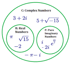
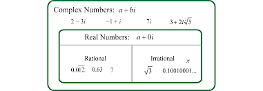
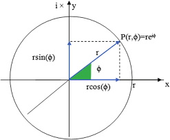
Recall that complex numbers $\mathrm{C}$ are expressions of the form $a+b \sqrt{-1}$, where $a$ and $b$ are real numbers. The number $\sqrt{-1}$ is defined to have the property $\sqrt{-1^{2}}=-1$. It is customary to use $i$ to denote $\sqrt{-1}$. Then, $i^{2}=-1$. Complex numbers written in the form $a+b i$ are said to be in standard form. In some instances it is convenient to write a complex number $a+b i$ in another form. To do this we represent $a+b i$ as the point $(a, b)$ in a plane coordinatized by a horizontal axis called the real axis and a vertical $i$ axis called the imaginary axis. The distance from the point $a+b i$ to the origin is $r=\sqrt{a^{2}+b^{2}}$ and is often denoted by $|a+b i|$ and called the norm of $a+b i$. If we draw the line segment from the origin to $a+b i$ and denote the angle formed by the line segment and the positive real axis by $\theta$, we can write $a+b i$ as $r(\cos \theta+i \sin \theta)$.
This form of $a+b i$ is called the polar form. An advantage of the polar form is demonstrated in parts 5 and 6 of Theorem 0.4.IEXAMPLE $11(-1+i)^{4}=\left(\sqrt{2}\left(\cos \frac{3 \pi}{4}+i \sin \frac{3 \pi}{4}\right)\right)^{4}=$ $\sqrt{2^{4}}\left(\cos \frac{4 \cdot 3 \pi}{4}+i \sin \frac{4 \cdot 3 \pi}{4}\right)=4(\cos 3 \pi+i \sin 3 \pi)=-4 .$ The three cube roots of $i=\cos \frac{\pi}{2}+i \sin \frac{\pi}{2}$ are $\cos \frac{\pi}{6}+i \sin \frac{\pi}{6}=\frac{\sqrt{3}}{2}+\frac{1}{2} i$ $\cos \left(\frac{\pi}{6}+\frac{2 \pi}{3}\right)+i \sin \left(\frac{\pi}{6}+\frac{2 \pi}{3}\right)=-\frac{\sqrt{3}}{2}+\frac{1}{2} i$ $\cos \left(\frac{\pi}{6}+\frac{4 \pi}{3}\right)+i \sin \left(\frac{\pi}{6}+\frac{4 \pi}{3}\right)=-i$.
PROOF We begin with the existence portion of the theorem. Consider the set $S={a-b k \mid k$ is an integer and $a-b k \geq 0}$. If $0 \in S$, then $b$ divides $a$ and we may obtain the desired result with $q=a / b$ and $r=0$. Now assume $0 \notin S$. Since $S$ is nonempty [if $a>0, a-b \cdot 0 \in S$; if $a<0, a-b(2 a)=a(1-2 b) \in S ; a \neq 0$ since $0 \notin S]$, we may apply the Well Ordering Principle to conclude that $S$ has a smallest member, say $r=a-b q$. Then $a=b q+r$ and $r \geq 0$, so all that remains to be proved is that $r<b$.
If $r \geq b$, then $a-b(q+1)=a-b q-b=r-b \geq 0$, so that $a-b(q+1) \in S$. But $a-b(q+1)<a-b q$, and $a-b q$ is the smallest member of $S$. So, $r<b$.
To establish the uniqueness of $q$ and $r$, let us suppose that there are integers $q, q^{\prime}, r$, and $r^{\prime}$ such that $$ a=b q+r, 0 \leq r<b, \text { and } a=b q^{\prime}+r^{\prime}, \quad 0 \leq r^{\prime}<b $$ For convenience, we may also suppose that $r^{\prime} \geq r$. Then $b q+$ $r=b q^{\prime}+r^{\prime}$ and $b\left(q-q^{\prime}\right)=r^{\prime}-r$. So, $b$ divides $r^{\prime}-r$ and $0 \leq r^{\prime}-r \leq r^{\prime}<b$. It follows that $r^{\prime}-r=0$, and therefore $r^{\prime}=r$ and $q=q^{\prime}$.
The integer $q$ in the division algorithm is called the quotient upon dividing $a$ by $b$; the integer $r$ is called the remainder upon dividing $a$ by $b$.
数学代写|抽象代数作业代写abstract algebra代考|GCD is a Linear Combination
PROOF Consider the set $S={a m+b n \mid m, n$ are integers and $a m+b n>0}$. Since $S$ is obviously nonempty (if some choice of $m$ and $n$ makes $a m+b n<0$, then replace $m$ and $n$ by $-m$ and $-n)$, the Well Ordering Principle asserts that $S$ has a smallest member, say, $d=a s+b t$. We claim that $d=\operatorname{gcd}(a, b)$. To verify this claim, use the division algorithm to write $a=d q+r$, where $0 \leq r0$, then $r=a-d \eta=a-(a s+b t) q=a-$ $a s q-b t q=a(1-s q)+b(-t q) \in S$, contradicting the fact that $d$ is the smallest member of $S$. So, $r=0$ and $d$ divides $a$. Analogously (or, better yet, by symmetry), $d$ divides $b$ as well. This proves that $d$ is a common divisor of $a$ and $b$. Now suppose $d^{\prime}$ is another common divisor of $a$ and $b$ and write $a=d^{\prime} h$ and $b=d^{\prime} k$. Then $d=a s+b t=\left(d^{\prime} h\right) s+\left(d^{\prime} k\right) t=d^{\prime}(h s+k t)$, so that $d^{\prime}$ is a divisor of $d$. Thus, among all common divisors of $a$ and $b, d$ is the greatest. The special case of Theorem $0.2$ when $a$ and $b$ are relatively prime is so important in abstract algebra that we single it out as a corollary.
■ EXAMPLE $2 \operatorname{gcd}(4,15)=1 ; \operatorname{gcd}(4,10)=2 ; \operatorname{gcd}\left(2^{2} \cdot 3^{2} \cdot 5,2 \cdot 3^{3}\right.$. $\left.7^{2}\right)=2 \cdot 3^{2}$. Note that 4 and 15 are relatively prime, whereas 4 and 10 are not. Also, $4 \cdot 4+15(-1)=1$ and $4(-2)+10 \cdot 1=2$. The corollary of Theorem $0.2$ provides a convenient method to show that two integers represented by polynomial expressions are relatively prime.
IEXAMPLE 3 For any integer $n$ the integers $n+1$ and $n^{2}+n+1$ are relatively prime. To verify this we observe that $n^{2}+n+1-$ $n(n+1)=1 .$
The next lemma is frequently used. It appeared in Euclid’s Elements.
数学代写|抽象代数作业代写abstract algebra代考|Notation for Arbitrary Groups
In group theory, we will regularly discuss the properties of an arbitrary group. In this case, instead of writing the operation as $a * b$, where * represents some unspecified binary operation, it is common to write the generic group operation as $a b$. With this convention of notation, it is also common to indicate the identity in an arbitrary group as 1 instead of $e$. In this chapter, however, we will continue to write $e$ for the arbitrary group identity in order to avoid confusion. Finally, with arbitrary groups, we denote the inverse of an element $a$ as $a^{-1} .$
This shorthand of notation should not surprise us too much. We already developed a similar habit with vector spaces. When discussing an arbitrary vector space, we regularly say, “Let $V$ be a vector space.” So though, in a strict sense, $V$ is only the set of the vector space, we implicitly understand that part of the information of a vector space is the addition of vectors (some operation usually denoted $+$ ) and the scalar multiplication of vectors.
By a similar abuse of language, we often refer, for example, to “the dihedral group $D_{n}$,” as opposed to “the dihedral group $\left(D_{n}, \circ\right)$.” Similarly, when we talk about “the group $\mathbb{Z} / n \mathbb{Z}$,” we mean $(\mathbb{Z} / n \mathbb{Z},+)$ because $(\mathbb{Z} / n \mathbb{Z}, \times)$ is not a group. And when we refer to “the group $U(n)$,” we mean the group $(U(n), \times)$. We will explicitly list the pair of set and binary operation if there could be confusion as to which binary operation the group refers. Furthermore, as we already saw with $D_{n}$, even if a group is equipped with a natural operation, we often just write $a b$ to indicate that operation. Following the analogy with multiplication, in a group $G$, if $a \in G$ and $k$ is a positive integer, by $a^{k}$ we mean $$ a^{k} \stackrel{\text { def }}{=} \overbrace{a a \cdots a}^{k \text { times }} . $$ We extend the power notation so that $a^{0}=e$ and $a^{-k}=\left(a^{-1}\right)^{k}$, for any positive integer $k$.
Groups that involve addition give an exception to the above habit of notation. In that case, we always write $a+b$ for the operation, $-a$ for the inverse, and, if $k$ is a positive integer, $$ k \cdot a \stackrel{\text { def }}{=} \overbrace{a+a+\cdots+a} . $$ We refer to $k \cdot a$ as a multiple of $a$ instead of as a power. Again, we extend the notation to nonpositive “multiples” just as above with powers.
数学代写|抽象代数作业代写abstract algebra代考|First Properties
The following proposition holds for any associative binary operation and does not require the other two axioms of group theory.
Proof. Before starting the proof, we define a temporary but useful notation. Given a sequence $a_{1}, a_{2}, \ldots, a_{k}$ of elements in $S$, by analogy with the $\sum$ notation, we define $$ \star_{i=1}^{k} a_{i} \stackrel{\text { def }}{=}\left(\cdots\left(\left(a_{1} \star a_{2}\right) \star a_{3}\right) \cdots a_{k-1}\right) \star a_{k} $$ In this notation, we perform the operations in (1.4) from left to right. Note that if $k=1$, the expression is equal to the element $a_{1}$.
We prove by (strong) induction on $n$, that every operation expression in $(1.4)$ is equal to $\boldsymbol{x}{i=1}^{n} a{i}$
The basis step with $n \geq 3$ is precisely the assumption that $\star$ is associative. We now assume that the proposition is true for all integers $k$ with $3 \leq$ $k \leq n$. Consider an operation expression (1.4) involving $n+1$ terms. Suppose without loss of generality that the last operation performed occurs between the $j$ th and $(j+1)$ th term, i.e.,
Since both operation expressions involve $n$ terms or less, by the induction hypothesis $$ q=\left(\star_{i=1}^{j} a_{i}\right) \star\left(\star_{i=j+1}^{n} a_{i}\right) . $$ Furthermore, $$ \begin{aligned} q &=\left(\star_{i=1}^{j} a_{i}\right) \star\left(a_{j+1} \star\left(\star_{i=j+2}^{n} a_{i}\right)\right) \quad \text { by the induction hypothesis } \ &=\left(\left(\star_{i=1}^{j} a_{i}\right) \star a_{j+1}\right) \star\left(\star_{i=j+2}^{n} a_{i}\right) \quad \text { by associativity } \ &=\left(\star_{i=1}^{j+1} a_{i}\right) \star\left(\star_{i=j+2}^{n} a_{i}\right) \end{aligned} $$ Repeating this $n-j-2$ more times, we conclude that $$ q=\star_{i=1}^{n+1} a_{i} $$ The proposition follows.
As we now jump into group theory with both feet, the reader might not immediately see the value in the definition of a group. The plethora of examples we provide subsequent to the definition will begin to showcase the breadth of applications. Definition 1.2.1 A group is a pair $(G, )$ where $G$ is a set and $$ is a binary operation on $G$ that satisfies the following properties: (1) associativity: $(a * b) * c=a *(b * c)$ for all $a, b, c \in G$; (2) identity: there exists $e \in G$ such that $a * e=e * a=a$ for all $a \in G$; (3) inverses: for all $a \in G$, there exists $b \in G$ such that $a * b=b * a=e$. By Proposition A.2.16, if any binary operation has an identity, then that identity is unique. Similarly, any element in a group has exactly one inverse element. Proposition 1.2.2 Let $(G, *)$ be a group. Then for all $a \in G$, there exists a unique inverse element to $a$.
Proof. Let $a \in G$ be arbitrary and suppose that $b_{1}$ and $b_{2}$ satisfy the properties of the inverse axiom for the element $a$. Then $$ \begin{aligned} b_{1} &=b_{1} * e & & \text { by identity axiom } \ &=b_{1} *\left(a * b_{2}\right) & & \text { by inverse axiom } \ &=\left(b_{1} * a\right) * b_{2} & & \text { by associativity } \ &=e * b_{2} & & \text { by definition of } b_{1} \ &=b_{2} & & \text { by identity axiom. } \end{aligned} $$ Therefore, for all $a \in G$ there exists a unique inverse. Since every group element has a unique inverse, our notation for inverses can reflect this. We denote the inverse element of $a$ by $a^{-1}$.
数学代写|抽象代数作业代写abstract algebra代考|A Few Examples
It is important to develop a robust list of examples of groups that show the breadth and restriction of the group axioms.
Example 1.2.4. The pairs $(\mathbb{Z},+),(\mathbb{Q},+),(\mathbb{R},+)$, and $(\mathbb{C},+)$ are groups. In each case, addition is associative and has 0 as the identity element. For a given element $a$, the additive inverse is $-a$.
Example 1.2.5. The pairs $\left(\mathbb{Q}^{}, \times\right),\left(\mathbb{R}^{}, \times\right)$, and $\left(\mathbb{C}^{}, \times\right)$ are groups. Recall that $A^{}$ mean $A-{0}$ when $A$ is a set that includes 0 . In each group, 1 is the multiplicative identity, and, for a given element $a$, the (multiplicative) inverse is $\frac{1}{a}$. Note that $\left(\mathbb{Z}^{*}, x\right)$ is not a group because it fails the inverse axiom. For example, there is no nonzero integer $b$ such that $2 b=1$.
On the other hand $\left(\mathbb{Q}^{>0}, x\right)$ and $\left(\mathbb{R}^{>0}, x\right)$ are groups. Multiplication is a binary operation on $\mathbb{Q}^{>0}$ and on $\mathbb{R}^{>0}$, and it satisfies all the axioms.
Example 1.2.6. A vector space $V$ is a group under vector addition with $\overrightarrow{0}$ as the identity. The (additive) inverse of a vector $\vec{v}$ is $-\vec{v}$. Note that the scalar multiplication of a vector spaces has no bearing on the group properties of vector addition.
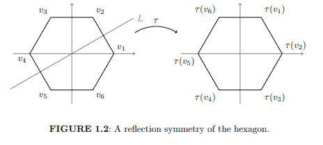
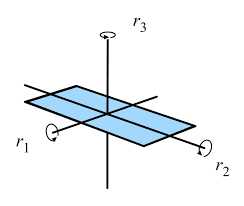
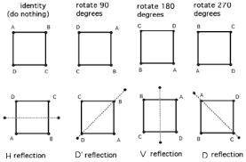
Let $n \geq 3$ and consider a regular $n$-sided polygon, $P_{n}$. Call $V=$ $\left{v_{1}, v_{2}, \ldots, v_{n}\right}$ the set of vertices of $P_{n}$ as a subset of the Euclidean plane $\mathbb{R}^{2}$. For simplicity, we often imagine the center of $P_{n}$ at the origin and that the vertex $v_{1}$ on the positive $x$-axis.
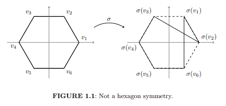
A symmetry of a regular $n$-gon is a bijection $\sigma: V \rightarrow V$ that is the restriction of a bijection $F: \mathbb{R}^{2} \rightarrow \mathbb{R}^{2}$, that leaves the overall vertex-edge structure of $P_{n}$ in place; i.e., if the unordered pair $\left{v_{i}, v_{j}\right}$ are the end points of an edge of the regular $n$-gon, then $\left{\sigma\left(v_{i}\right), \sigma\left(v_{j}\right)\right}$ is also an edge.
Consider, for example, a regular hexagon $P_{6}$ and the bijection $\sigma: V \rightarrow V$ such that $\sigma\left(v_{1}\right)=v_{2}, \sigma\left(v_{2}\right)=v_{1}$, and $\sigma$ stays fixed on all the other vertices. Then $\sigma$ is not a symmetry of $P_{6}$ because it fails to preserve the vertex-edge structure of the hexagon. As we see in Figure $1.1$, though $\left{v_{2}, v_{3}\right}$ is an edge of the hexagon, while $\left{\sigma\left(v_{2}\right), \sigma\left(v_{3}\right)\right}$ are not the endpoints of an edge of the hexagon.
To count the number of bijections on the set $V=\left{v_{1}, v_{2}, \ldots, v_{n}\right}$, we note that a bijection $f: V \rightarrow V$ can map $f\left(v_{1}\right)$ to any element in $V$; then it can map $f\left(v_{2}\right)$ to any element in $V \backslash\left{f\left(v_{1}\right)\right}$; then it can map $f\left(v_{3}\right)$ to any element in $V \backslash\left{f\left(v_{1}\right), f\left(v_{2}\right)\right}$; and so on. Hence, there are $$ n \times(n-1) \times(n-2) \times \cdots \times 2 \times 1=n ! $$ distinct bijections on $V$. However, a symmetry $\sigma \in D_{n}$ can map $\sigma\left(v_{1}\right)$ to any element in $V(n$ options), but then $\sigma$ must map $v_{2}$ to a vertex adjacent to $\sigma\left(v_{1}\right)$ (2 options). Once $\sigma\left(v_{1}\right)$ and $\sigma\left(v_{2}\right)$ are known, all remaining $\sigma\left(v_{i}\right)$ for $3 \leq i \leq n$ are determined. In particular, $\sigma\left(v_{3}\right)$ must be the vertex adjacent to $\sigma\left(v_{2}\right)$ that is not $\sigma\left(v_{1}\right) ; \sigma\left(v_{4}\right)$ must be the vertex adjacent to $\sigma\left(v_{3}\right)$ that is not $\sigma\left(v_{2}\right)$; and so on. This reasoning leads to the following proposition.
数学代写|抽象代数作业代写abstract algebra代考|Abstract Notation
We introduce a notation that is briefer and aligns with the abstract notation that we will regularly use in group theory.
Having fixed an integer $n \geq 3$, denote by $r$ the rotation of angle $2 \pi / n$, by $s$ the reflection through the $x$-axis, and by $\iota$ the identity function. In other words, $$ r=R_{2 \pi / n}, \quad s=F_{0}, \quad \text { and } \quad \iota=R_{0} \text {. } $$ In abstract notation, similar to our habit of notation for multiplication of real variables, we write $a b$ to mean $a \circ b$ for two elements $a, b \in D_{n}$. Borrowing from a theorem in the next section (Proposition 1.2.13), since $\circ$ is associative, an expression such as $r r s r$ is well-defined, regardless of the order in which we pair terms to perform the composition. In this example, with $n=4$, $$ r r s r=R_{\pi / 2} \circ R_{\pi / 2} \circ F_{0} \circ R_{\pi / 2}=R_{\pi} \circ F_{0} \circ R_{\pi / 2}=F_{\pi / 2} \circ R_{\pi / 2}=F_{\pi / 4} . $$ To simplify notations, if $a \in D_{n}$ and $k \in \mathbb{N}^{*}$, then we write $a^{k}$ to represent $$ a^{k}=\overbrace{a a a \cdots a}^{k \text { times }} . $$ Hence, we write $r^{2} s r$ for $r r s r$. Since composition o is not commutative, $r^{3} s$ is not necessarily equal to $r^{2} s r$. From Proposition 1.1.3, it is not hard to see that $$ r^{k}=R_{2 \pi k / n} \quad \text { and } \quad r^{k} s=F_{\pi k / n} $$ where $k$ satisfies $0 \leq k \leq n-1$. Consequently, as a set $$ D_{n}=\left{\iota, r, r^{2}, \ldots, r^{n-1}, s, r s, r^{2} s, \ldots, r^{n-1} s\right} $$ The symbols $r$ and $s$ have a few interesting properties. First, $r^{n}=\iota$ and $s^{2}=\iota$. These are obvious as long as we do not forget the geometric meaning of the functions $r$ and $s$. Less obvious is the equality in the following proposition.
让 $n \geq 3$ 并考虑一个常规的 $n$ 边多边形, $P_{n}$. 称呼 $V=\mathrm{~ l e f t { v _ { 1 } , ~ V _ { 2 } , ~ V d o t s , ~ V _ { { n }}$ 得平面的子集 $\mathbb{R}^{2}$. 为简单起见,我们经常想象 $P_{n}$ 在原点和那个顶点 $v_{1}$ 在积极的 $x$-轴。 正则对称 $n$-gon 是双射 $\sigma: V \rightarrow V$ 这是双射的限制 $F: \mathbb{R}^{2} \rightarrow \mathbb{R}^{2}$ ,这留下了整体的顶点边缘结构 $P_{n}$ 到位; 即, 如果无序对 Vleft{v_{{i}, v_{j}\right} 是正则的一条边的端点 $n$-gon,然后 $\mathrm{~ ע l e f t { \ s i g m a l l e f t ( v _ { i }}$ 例如,考虑一个正六边形 $P_{6}$ 和双射 $\sigma: V \rightarrow V$ 这样 $\sigma\left(v_{1}\right)=v_{2}, \sigma\left(v_{2}\right)=v_{1}$ , 和 $\sigma$ 保持固定在所有其他顶点 上。然后 $\sigma$ 不是对称的 $P_{6}$ 因为它末能保留六边形的顶点边缘结构。如图所示 $1.1$ ,尽管 left{v_{{2}, V__{3}\right } } \text { 是六 } $\mathrm{~ 边 形 的 一 条 边 , 而 l l e f t { \ s i g m a l l e f t ( v _ { 2 } | r i g h t ) , ~ I s i g m a l l e f t ( v _ { ( 3 }}$ 任何元素 $V$; 然后它可以映射 $f\left(v_{2}\right) \mathrm{~ 中 的 任 何 元 素 ⿰ V ⿱ ⺌}$ 的任何元素 $V \mathrm{~ \ b a c k s l a s h l l e f t ( f ) l e f t ( V _ { { 1 } \ r i g h t ) , ~ f ^ l e f t (}$ $$ n \times(n-1) \times(n-2) \times \cdots \times 2 \times 1=n ! $$ 不同的双射 $V$. 然而,对称 $\sigma \in D_{n}$ 可以映射 $\sigma\left(v_{1}\right)$ 中的任何元素 $V\left(n\right.$ 选项),但随后 $\sigma$ 必须映射 $v_{2}$ 到相邻的顶点 $\sigma\left(v_{1}\right)$ (2 个选 项)。一次 $\sigma\left(v_{1}\right)$ 和 $\sigma\left(v_{2}\right)$ 是已知的,所有剩余的 $\sigma\left(v_{i}\right)$ 为了 $3 \leq i \leq n$ 被确定。尤其是, $\sigma\left(v_{3}\right)$ 必须是相邻的顶 点 $\sigma\left(v_{2}\right)$ 那不是 $\sigma\left(v_{1}\right) ; \sigma\left(v_{4}\right)$ 必须是相邻的顶点 $\sigma\left(v_{3}\right)$ 那不是 $\sigma\left(v_{2}\right)$; 等等。这个推理导致了以下命题。
数学代写|抽象代数作业代写abstract algebra代考|History of Ring Theory
数学代写|抽象代数作业代写abstract algebra代考|Noncommutative ring theory
Algebra textbooks usually give the definition of a ring first and follow it with examples. Of course the examples came first, and the abstract definition later-much later. So we begin with examples.
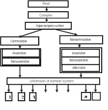
Among the most important examples of rings are the integers, polynomials, and matrices. “Simple” extensions of these examples are at the roots of ring theory. Specifically, we have in mind the following three examples: (a) The integers $Z$ can be thought of as the appropriate subdomain of the field $Q$ of rationals in which to do number theory. (The rationals themselves are unsuitable for that purpose: every rational is divisible by every other (nonzero) rational.) Take a simple extension field $Q(\alpha)$ of the rationals, where $\alpha$ is an algebraic number, that is, a root of a polynomial with integer coefficients. $Q(\alpha)$ is called an algebraic number field; it consists of polynomials in $\alpha$ with rational coefficients. For example, $Q(\sqrt{3})={a+b \sqrt{3}: a, b \in Q}$.
The appropriate subdomain of $Q(\alpha)$ in which to do number theory -the “integers” of $Q(\alpha)$-consists of those elements that are roots of monic polynomials with integer coefficients, polynomials $p(x)$ in which the coefficient of the highest power of $x$ is 1 . For example, the integers of $Q(\sqrt{3})$ are ${a+b \sqrt{3}: a, b \in Z}$ (this is not obvious). This is our first example. (b) The polynomial rings $\mathbf{R}[x]$ and $\mathbf{R}[x, y]$ in one and in two variables, respectively, share important properties but also differ in significant ways ( $\mathbf{R}$ denotes the real numbers). In particular, while the roots of a polynomial in one variable constitute a discrete set of real numbers, the roots of a polynomial in two variables constitute a curve in the plane-a so-called algebraic curve. Our second example, then, is the ring of polynomials in two (or more) variables. (c) Square $m \times m$ matrices (for example, over the reals) can be viewed as $m^{2}$ tuples of real numbers with coordinate-wise addition and appropriate multiplication obeying the axioms of a ring. Our third example consists, more generally, of $n$-tuples $\mathbf{R}^{n}$ of real numbers with coordinate-wise addition and appropriate multiplication, so that the resulting system is a (not necessarily commutative) ring. Such systems, often extensions of the complex numbers, were called in the nineteenth and early twentieth centuries hypercomplex number systems.
In what contexts did these examples arise? What was their importance? The answers will lead us to the genesis of ring theory.
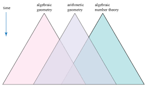
Rings fall into two broad categories: commutative and noncommutative. The abstract theories of these two categories came from distinct sources and developed in different directions. Commutative ring theory originated in algebraic number theory, algebraic geometry, and invariant theory. Central to the development of these subjects were the rings of integers in algebraic number fields and algebraic function fields, and the rings of polynomials in two or more variables.
Noncommutative ring theory began with attempts to extend the complex numbers to various hypercomplex number systems. The genesis of the theories of commutative and noncommutative rings dates back to the early nineteenth century, while their maturity was achieved only in the third decade of the twentieth century. The following is a diagrammatic sketch of the above remarks.
数学代写|抽象代数作业代写abstract algebra代考|Examples of Hypercomplex Number Systems
Hamilton’s invention of the quaternions was conceptually groundbreaking-_”a revolution in arithmetic which is entirely similar to the one which Lobachevsky effected
in geometry,” according to Poincaré. Indeed, both achievements were radical violations of prevailing conceptions. Like all revolutions, however, the invention of the quaternions was initially received with less than universal approbation: “I have not yet any clear view as to the extent to which we are at liberty arbitrarily to create imaginaries, and to endow them with supernatural properties,” declared Hamilton’s mathematician friend John Graves.
Most mathematicians, however, including Graves, soon came around to Hamilton’s point of view. The quaternions acted as a catalyst for the exploration of diverse “number systems,” with properties which departed in various ways from those of the real and complex numbers. Among the examples of such hypercomplex number systems are the following: (i) Octonions These are 8-tuples of reals which contain the quaternions and form a division algebra in which multiplication is nonassociative. They were introduced in 1844 by Cayley and independently by the very John Graves who questioned Hamilton’s “imaginaries.” (ii) Exterior algebras These are $n$-tuples of reals, added componentwise and multiplied via the “exterior product.” They were introduced by Grassmann in 1844 as part of a brilliant attempt to construct a vector algehra in $n$-dimensional space. Grassmann’s style was far from simple and his approach was ahead of its time. (iii) Group algebras In 1854 Cayley published a paper on (finite) abstract groups, at the end of which he gave a definition of a group algebra (over the real or complex numbers). He called it a system of “complex quantities” and observed that it is analogous to Hamilton’s quaternions-it is associative, noncommutative, but in general not a division algebra. (iv) Matrices In two papers of 1855 and 1858 Cayley introduced square matrices. He noted that they can be treated as “single quantities,” added and multiplied like “ordinary algebraic quantities,” but that “as regards their multiplication, there is the peculiarity that matrices are not in general convertible [commutative].” See Chapter 5.1.3.
数学代写|抽象代数作业代写abstract algebra代考|Classification
Over a thirty-year period (c. $1840-1870$ ) a stock of examples of noncommutative number systems had been established. One could now begin to construct a theory. The general concept of a hypercomplex number system (in current terminology, a finite-dimensional algebra) emerged, and work began on classifying certain types
of these structures. We focus on three such developments, dealing with associative algebras. Note that such algebras are, of course, rings. (i) Low-dimensional algebras Of fundamental importance here was the work of Benjamin Peirce of Harvard-the first important contribution to algebra in the U.S. We are referring to his groundbreaking paper “Linear Associative Algebra” of 1870. In the last 100 pages of this 150-page paper Peirce classified algebras (i.e., hypercomplex number systems) of dimension $<6$ by giving their multiplication tables. There are, he showed, over 150 such algebras! What is important in this paper, though, is not the classification but the means used to obtain it. For here Peirce introduced concepts, and derived results, which proved fundamental for subsequent developments. Among these conceptual advances were:
(a) An “abstract” definition of a finite-dimensional algebra. Peirce defined such an algebra-he called it a “linear associative algebra”-as the totality of formal expressions of the form $\sum_{i=1}^{n} a_{i} e_{i}$, where the $e_{i}$ are “basis elements.” Addition was defined componentwise and multiplication by means of “structural constants” $c_{i j k}$, namely $e_{i} e_{j}=\sum_{k=1}^{n} c_{i j k} e_{k}$. Associativity under multiplication and distributivity were postulated, but not commutativity. This is probably the earliest explicit definition of an associative algebra. (b) The use of complex coefficients. Peirce took the coefficients $a_{i}$ in the expressions $\sum a_{i} e_{i}$ to be complex numbers. This conscious broadening of the field of coefficients from $\mathbf{R}$ to $\mathbf{C}$ was an important conceptual advance on the road to coefficients taken from an arbitrary field. (c) Relaxation of the requirement that an algebra have an identity. This, too, was a departure from past practice and gave an indication of Peirce’s general, abstract approach.
数学代写|抽象代数作业代写abstract algebra代考|History of Ring Theory
数学代写|抽象代数作业代写abstract algebra代考|Emergence of abstraction in group theory
数学代写|抽象代数作业代写abstract algebra代考|Emergence of abstraction in group theory
The abstract point of view in group theory emerged slowly. It took over one hundred years from the time of Lagrange’s implicit group-theoretic work of 1770 for the abstract group concept to evolve. E. T. Bell discerns several stages in this process of evolution towards abstraction and axiomatization: The entire development required about a century. Its progress is typical of the evolution of any major mathematical discipline of the recent period; first, the discovery of isolated phenomena; then the recognition of certain features common to all; next the search for further instances, their detailed calculation and classification; then the emergence of general principles making further calculations, unless needed for some definite application, superfluous; and last, the formulation of postulates crystallizing in abstract form the structure of the system investigated [2].
Although somewhat oversimplified, as all such generalizations tend to be, this is nevertheless a useful framework. Indeed, in the case of group theory, first came the “isolated phenomena”-for example, permutations, binary quadratic forms, roots of unity; then the recognition of “common features”-the concept of a finite group, encompassing both permutation groups and finite abelian groups (cf. the paper of Frobenius and Stickelberger cited above); next the search for “other instances”-in our case transformation groups; and finally the formulation of “postulates”-in this case the postulates of a group, encompassing both the finite and infinite cases. We now consider when and how the intermediate and final stages of abstraction occurred. In 1854 Cayley gave the first abstract definition of a finite group in a paper entitled “On the theory of groups, as depending on the symbolic equation $\theta^{n}=1 . “$ (In 1858 Dedekind, in lectures on Galois theory at Göttingen, gave another. See 8.2.) Here is Cayley’s definition: A set of symbols $1, \alpha, \beta, \ldots$, all of them different, and such that the product of any two of them (no matter in what order), or the product of any one of them into itself, belongs to the set, is said to be a group. Cayley went on to say that: These symbols are not in general convertible [commutative] but are associative … and it follows that if the entire group is multiplied by any one of the symbols, either as further or nearer factor [i.e., on the left or on the right], the effect is simply to reproduce the group [33]. He then presented several examples of groups, such as the quaternions (under addition), invertible matrices (under multiplication), permutations, Gauss’ quadratic forms, and groups arising in elliptic function theory. Next he showed that every abstract group is (in our terminology) isomorphic to a permutation group, a result now known as Cayley’s theorem.
数学代写|抽象代数作业代写abstract algebra代考|Consolidation of the abstract group concept
The abstract group concept spread rapidly during the $1880 \mathrm{~s}$ and $1890 \mathrm{~s}$, although there still appeared a great many papers in the areas of permutation and transformation
groups. The abstract viewpoint was manifested in two ways: (a) Concepts and results introduced and proved in the setting of “concrete” groups were now reformulated and reproved in an abstract setting; (b) Studies originating in, and based on, an abstract setting began to appear. An interesting example of the former case is the reproving by Frobenius, in an abstract setting, of Sylow’s theorem, which was proved by Sylow in 1872 for permutation groups. This was done in 1887, in a paper entitled “A new proof of Sylow’s theorem.” Although Frobennius admitted that the fact that every finite group can be repreesented by a group of permutations proves that Sylow’s theorem must hold for all finite groups, he nevertheless wished to establish the theorem abstractly: Since the symmetric group, which is introduced into all these proofs, is totally alien to the context of Sylow’s theorem, I have tried to find a new derivation of it. For a case study of the evolution of abstraction in group theory in connection with Sylow’s theorem see [28] and [32].
Hölder was an important contributor to abstract group theory, and was responsible for introducing a number of group-theoretic concepts abstractly. For example, in 1889 he defined the abstract notion of a quotient group. The quotient group was first seen as the group of the “auxiliary equation,” later as a homomorphic image, and only in Hölder’s time as a group of cosets. He then “completed” the proof of the JordanHölder theorem, namely that the quotient groups in a composition series are invariant up to isomorphism (see Jordan’s contribution, p. 25). For a history of the concept of quotient group see [36].
In 1893 , in a paper on groups of order $p^{3}, p q^{2}, p q r$, and $p^{4}$, Holder introduced the concept of an automorphism of a group abstractly. He was also the first to study simple groups abstractly. (Previously they were considered in concrete cases-as permutation groups, transformation groups, and so on.) As he said: “It would be of the greatest interest if a survey of all simple groups with a finite number of operations could be known.” (By “operations” Hölder meant “elements.”) He then went on to determine the simple groups of order up to 200 .
数学代写|抽象代数作业代写abstract algebra代考|Divergence of developments in group theory
Group theory evolved from several different sources, giving rise to various concrete theories. These theories developed independently, some for over one hundred years, beginning in 1770 , before they converged in the early 1880 s within the abstract group concept. Abstract group theory emerged and was consolidated in the next thirty to forty years. At the end of that period (around 1920) one can discern the divergence of group theory into several distinct “theories.” Here is the barest indication of some of these advances and new directions in group theory, beginning in the $1920 \mathrm{~s}$, with the names of some of the major contributors and approximate dates: (a) Finite group theory. The major problem here, already formulated by Cayley in the 1870 s and studied by Jordan and Hölder. was to find all finite groups of a given order. The problem proved too difficult and mathematicians turned to special cases, suggested especially by Galois theory: to find all simple or all solvable groups (cf. the Feit-Thompson theorem of 1963 , and the classification of all finite simple groups in 1981). See [14], [15], [30].
数学代写|抽象代数作业代写abstract algebra代考|Emergence of abstraction in group theory
数学代写|抽象代数作业代写abstract algebra代考|Development of “specialized” theories of groups
数学代写|抽象代数作业代写abstract algebra代考|Permutation Groups
As noted earlier, Lagrange’s work of 1770 initiated the study of permutations in connection with the study of the solution of equations. It was probably the first clear instance of implicit group-theoretic thinking in mathematics. It led directly to the $\mathrm{~ w o ̄ ̄ i k s ̄ ~ o ̂ f ~ K u ̈ f f i n ̃ i , ~ A ̊ b e ́ l , ~ a ̄ n đ ~ G a ̄ l o ̄ i s ~ đ u ̈}$ to the concept of a permutation group.
Ruffini and Abel proved the unsolvability of the quintic by building on the ideas of Lagrange concerning resolvents. Lagrange showed that a necessary condition for the solvability of the general polynomial equation of degree $n$ is the existence of a resolvent of degree less than $n$. Ruffini and Abel showed that such resolvents do not exist for $n>4$. In the process they developed elements of permutation theory. It was Galois, however, who made the fundamental conceptual advances, and who is considered by many as the founder of (permutation) group theory.
He was familiar with the works of Lagrange, Abel, and Gauss on the solution of polynomial equations. But his aim went well beyond finding a method for solvability of equations. He was concerned with gaining insight into general principles, dissatisfied as he was with the methods of his predecessors: “From the beginning of this century,” he wrote, “computational procedures have become so complicated that any progress by those means has become impossible.”
Galois recognized the separation between “Galois theory”-the correspondence between fields and groups-and its application to the solution of equations, for he wrote that he was presenting “the general principles and just one application” of the theory. “Many of the early commentators on Galois theory failed to recognize this distinction, and this led to an emphasis on applications at the expense of the theory” [19].
Galois was the first to use the term “group” in a technical sense-to him it signified a collection of permutations closed under multiplication: “If one has in the same group the substitutions $S$ and $T$, one is certain to have the substitution $S T$.” He recognized that the most important properties of an algebraic equation were reflected in certain properties of a group uniquely associated with the equation-“the group of the equation.” To describe these properties he invented the fundamental notion of normal subgroup and used it to great effect.
While the issue of resolvent equations preoccupied Lagrange, Ruffini, and Abel, Galois’ basic idea was to bypass them, for the construction of a resolvent required great skill and was not based on a clear methodology. Galois noted instead that the existence of a resolvent was equivalent to the existence of a normal subgroup of prime index in the group of the equation. This insight shifted consideration from the resolvent equation to the group of the equation and its subgroups. Galois defined the group of an equation as follows: Let an equation be given, whose $m$ roots are $a, b, c, \ldots .$ There will always be a group of permutations of the letters $a, b, c, \ldots$ which has the following property: (1) that every function of the roots, invariant under the substitutions of that group, is rationally known [i.e., is a rational function of the coefficients and any adjoined quantities]; (2) conversely, that every function of the roots, which can be expressed rationally, is invariant under these substitutions [19].
数学代写|抽象代数作业代写abstract algebra代考|Abelian Groups
As noted earlier, the main source for abelian group theory was number theory, beginning with Gauss’ Disquisitiones Arithmeticae. (Note also implicit abelian group theory in Euler’s number-theoretic work [33].) In contrast to permutation theory, grouptheoretic modes of thought in number theory remained implicit until about the last third of the nineteenth century. Until that time no explicit use of the term “group” was made, and there was no link to the contemporary, flourishing theory of permutation groups. We now give a sample of some implicit group-theoretic work in number theory, especially in algebraic number theory.
Algebraic number theory arose in connection with Fermat’s Last Theorem, the insolvability in nonzero integers of $x^{n}+y^{n}=z^{n}$ for $n>2$, Gauss’ theory of binary quadratic forms, and higher reciprocity laws (see Chapter 3.2). Algebraic number fields and their arithmetical properties were the main objects of study. In 1846 Dirichlet studied the units in an algebraic number field and established that (in our terminology) the group of these units is a direct product of a finite cyclic group and a free abelian group of finite rank. At about the same time Kummer introduced his “ideal numbers,” defined an equivalence relation on them, and derived, for cyclotomic fields, certain special properties of the number of equivalence classes, the so-called class number of a cyclotomic field-in our terminology, the order of the ideal class group of the cyclotomic field. Dirichlet had earlier made similar studies of quadratic fields. In 1869 Schering, a former student of Gauss, investigated the structure of Gauss’ (group of) equivalence classes of binary quadratic forms (see Chapter 3 ). He found certain fundamental classes from which all classes of forms could be obtained by composition. In group-theoretic terms, Schering found a basis for the abelian group of equivalence classes of binary quadratic forms.
数学代写|抽象代数作业代写abstract algebra代考|Transformation Groups
As in number theory, so in geometry and analysis, group-theoretic ideas remained implicit until the last third of the nineteenth century. Moreover, Klein’s (and Lie’s) explicit use of groups in geometry influenced the evolution of group theory concep tually rather than technically. It signified a genuine shift in the development of group theory from a preoccupation with permutation groups to the study of groups of transformations. (That is not to suggest, of course, that permutation groups were no longer studied.) This transition was also notable in that it pointed to a turn from finite groups to infinite groups.
Klein noted the connection of his work with permutation groups but also realized the departure he was making. He stated that what Galois theory and his own program have in common is the investigation of “groups of changes,” but added that “to be sure,
the objects the changes apply to are different: there [Galois theory] one deals with a finite number of discrete elements, whereas here one deals with an infinite number of elements of a continuous manifold.”‘ To continue the analogy, Klein noted that just as there is a theory of permutation groups, “we insist on a theory of transformations, a study of groups generated by transformations of a given type.”
Klein shunned the abstract point of view in group theory, and even his technical definition of a (transformation) group is deficient: Now let there be given a sequence of transformations $A, B, C, \ldots .$ If this sequence has the property that the composite of any two of its transformations yields a transformation that again belongs to the sequence, then the latter will be called a group of transformations [33]. Klein’s work, however, broadened considerably the conception of a group and its applicability in other fields of mathematics. He did much to promote the view that group-theoretic ideas are fundamental in mathematics: The special subject of group theory extends through all of modern mathematics. As an ordering and classifying principle, it intervenes in the most varied domains.
数学代写|抽象代数作业代写abstract algebra代考|Development of “specialized” theories of groups
Ruffini 和 Abel 通过建立拉格朗日关于分解的思想证明了五次方程的不可解性。拉格朗日证明了一般多项式度方程的可解性的必要条件n是否存在度数小于的解析器n. Ruffini 和 Abel 表明此类解决方案不存在n>4. 在这个过程中,他们发展了置换理论的元素。然而,是伽罗瓦在概念上取得了根本性的进步,并且被许多人认为是(置换)群论的创始人。
数学代写|抽象代数作业代写abstract algebra代考|Sources of group theory
数学代写|抽象代数作业代写abstract algebra代考|Classical Algebra
The major problems in algebra at the time $(1770)$ that Lagrange wrote his fundamental memoir “Reflections on the solution of algebraic equations” concerned polynomial equations. There were “theoretical” questions dealing with the existence and nature of the roots-for example, does every equation have a root? how many roots are there? are they real, complex, positive, negative?-and “practical” questions dealing with methods for finding the roots. In the latter instance there were exact methods and approximate methods. In what follows we mention exact methods.
The Babylonians knew how to solve quadratic equations, essentially by the method of completing the square, around $1600 \mathrm{BC}$ (see Chapter 1). Algebraic methods for solving the cubic and the quartic were given around 1540 (Chapter 1). One of the major problems for the next two centuries was the algebraic solution of the quintic. This is the task Lagrange set for himself in his paper of 1770 .In this paper Lagrange first analyzed the various known methods, devised by Viète, Descartes, Euler, and Bezout, for solving cubic and quartic equations. He showed that the common feature of these methods is the reduction of such equations to auxiliary equations-the so-called resolvent equations. The latter are one degree lower than the original equations.
Lagrange next attempted a similar analysis of polynomial equations of arbitrary degree $n$. With each such equation he associated a resolvent equation, as follows: let $f(x)$ be the original equation, with roots $x_{1}, x_{2}, x_{3}, \ldots, x_{n}$. Pick a rational function $\mathbf{R}\left(x_{1}, x_{2}, x_{3}, \ldots, x_{n}\right)$ of the roots and coefficients of $f(x)$. (Lagrange described methods for doing this.) Consider the different values which $\mathbf{R}\left(x_{1}, x_{2}, x_{3}, \ldots, x_{n}\right)$ assumes under all the $n$ ! permutations of the roots $x_{1}, x_{2}, x_{3}, \ldots, x_{n}$ of $f(x)$. If these are denoted by $y_{1}, y_{2}, y_{3}, \ldots, y_{k}$, then the resolvent equation is given by $g(x)=\left(x-y_{1}\right)\left(x-y_{2}\right) \cdots\left(x-y_{k}\right) .$
It is imporotant to note that the coefficients of $g(x)$ aree symmetric functions in $x_{1}, x_{2}, x_{3}, \ldots, x_{n}$, hence they are polynomials in the elementary symmetric functions of $x_{1}, x_{2}, x_{3}, \ldots, x_{n}$; that is, they are polynomials in the coefficients of the original equation $f(x)$. Lagrange showed that $k$ divides $n$ !-the source of what we call Lagrange’s theorem in group theory.
For example, if $f(x)$ is a quartic with roots $x_{1}, x_{2}, x_{3}, x_{4}$, then $\mathbf{R}\left(x_{1}, x_{2}, x_{3}, x_{4}\right)$ may be taken to be $x_{1} x_{2}+x_{3} x_{4}$, and this function assumes three distinct values under the twenty-four permutations of $x_{1}, x_{2}, x_{3}, x_{4}$. Thus the resolvent equation of a quartic is a cubic. However, in carrying over this analysis to the quintic Lagrange found that the resolvent equation is of degree six.
Although Lagrange did not succeed in resolving the problem of the algebraic solvability of the quintic, his work was a milestone. It was the first time that an association was made between the solutions of a polynomial equation and the permutations of its roots. In fact, the study of the permutations of the roots of an equation was a cornerstone of Lagrange’s general theory of algebraic equations. This, he speculated, formed “the true principles of the solution of equations.” He was, of course, vindicated in this by Galois. Although Lagrange spoke of permutations without considering a “calculus” of permutations (e.g., there is no consideration of their composition or closure), it can be said that the germ of the group concept-as a group of permutations-is present in his work. For details see [12], [16], [19], [25], [33].
数学代写|抽象代数作业代写abstract algebra代考|Number Theory
In the Disquisitiones Arithmeticae (Arithmetical Investigations) of 1801 Gauss summarized and unified much of the number theory that preceded him. The work also suggested new directions which kept mathematicians occupied for the entire century. As for its impact on group theory, the Disquisitiones may be said to have initiated the theory of finite abelian groups. In fact, Gauss established many of the significant properties of these groups without using any of the terminology of group theory. The groups appeared in four different guises: the additive group of integers modulo $m$, the multiplicative group of integers relatively prime to $m$, modulo $m$, the group of equivalence classes of binary quadratic forms, and the group of $n$-th roots of unity. And although these examples turned up in number-theoretic contexts, it is as abelian groups that Gauss treated them, using what are clear prototypes of modern algebraic proofs.
For example, considering the nonzero integers modulo $p$ ( $p$ a prime), he showed that they are all powers of a single element; that is, that the group $Z_{p}^{*}$ of such integers
is cyclic. Moreover, he determined the number of generators of this group, showing that it is equal to $\varphi(p-1)$, where $\varphi$ is Euler’s $\varphi$-function.
Given any element of $Z_{p}^{}$, he defined the order of the element (without using the terminology) and showed that the order of an element is a divisor of $p-1$. He then used this result to prove Fermat’s “little theorem,” namely that $a^{p-1} \equiv 1(\bmod p)$ if $p$ does not divide $a$, thus employing group-theoretic ideas to prove number-theoretic results. Next he showed that if $t$ is a positive integer which divides $p-1$, then there exists an element in $Z_{p}^{}$ whose order is $t$-essentially the converse of Lagrange’s theorem for cyclic groups.
Concerning the $n$-th roots of 1 , which he considered in connection with the cyclotomic equation, he showed that they too form a cyclic group. In relation to this group he raised and answered many of the same questions he raised and answered in the case of $Z_{p}^{*}$.
The problem of representing integers by binary quadratic forms goes back to Fermat in the early seventeenth century. (Recall his theorem that every prime of the form $4 n+1$ can be represented as a sum of two squares $x^{2}+y^{2}$.) Gauss devoted a large part of the Disquisitiones to an exhaustive study of binary quadratic forms and the representation of integers by such forms.
A binary quadratic form is an expression of the form $a x^{2}+b x y+c y^{2}$, with $a, b, c$ integers. Gauss defined a composition on such forms, and remarked that if $K_{1}$ and $K_{2}$ are two such forms, one may denote their composition by $K_{1}+K_{2}$. He then showed that this composition is associative and commutative, that there exists an identity, and that each form has an inverse, thus verifying all the properties of an abelian group.
Despite these remarkable insights, one should not infer that Gauss had the concept of an abstract group, or even of a finite abelian group. Although the arguments in the Disquisitiones are quite general, each of the various types of “groups” he considered was dealt with separately-there was no unifying group-theoretic method which he applied to all cases. For further details see [5], [9], [25], [30], [33].
数学代写|抽象代数作业代写abstract algebra代考|Geometry
We are referring here to Klein’s famous and influential (but see [18]) lecture entitled “A Comparative Review of Recent Researches in Geometry,” which he delivered in 1872 on the occasion of his admission to the faculty of the University of Erlangen. The aim of this so-called Erlangen Program was the classification of geometry as the study of invariants under various groups of transformations. Here there appear groups such as the projective group, the group of rigid motions, the group of similarities, the hyperbolic group, the elliptic groups, as well as the geometries associated with them. (The affine group was not mentioned by Klein.) Now for some background leading to Klein’s Erlangen Program.
The nineteenth century witnessed an explosive growth in geometry, both in scope and in depth. New geometries emerged: projective geometry, noneuclidean geometries, differential geometry, algebraic geometry, $n$-dimensional geometry, and
Grassmann’s geometry of extension. Various geometric methods competed for supremacy: the synthetic versus the analytic, the metric versus the projective.
At mid-century a major problem had arisen, namely the classification of the relations and inner connections among the different geometries and geometric methods. This gave rise to the study of “geometric relations,” focusing on the study of properties of figures invariant under transformations. Soon the focus shifted to a study of the transformations themselves. Thus the study of the geometric relations of figures became the study of the associated transformations.
Various types of transformations (e.g., collineations, circular transformations, inversive transformations, affinities) became the objects of specialized studies. Subsequently, the logical connections among transformations were investigated, and this led to the problem of classifying transformations, and eventually to Klein’s group-theoretic synthesis of geometry.
Klein’s use of groups in geometry was the final stage in bringing order to geometry. An intermediate stage was the founding of the first major theory of classification in geometry, beginning in the $1850 \mathrm{~s}$, the Cayley-Sylvester Invariant Theory. Here the objective was to study invariants of “forms” under transformations of their variables (see Chapter 8.1). This theory of classification, the precursor of Klein’s Erlangen Program, can be said to be implicitly group-theoretic. Klein’s use of groups in geometry was, of course, explicit. (For a thorough analysis of implicit group-theoretic thinking in geometry leading to Klein’s Erlangen Program see [33].)
In the next section we will note the significance of Klein’s Erlangen Program (and his other works) for the evolution of group theory. Since the Program originated a hundred years after Lagrange’s work and eighty years after Gauss’ work, its importance for group theory can best be appreciated after a discussion of the evolution of group theory beginning with the works of Lagrange and Gauss and ending with the period around 1870 .
数学代写|抽象代数作业代写abstract algebra代考|Sources of group theory