如果你也在 怎样代写复分析Complex function这个学科遇到相关的难题，请随时右上角联系我们的24/7代写客服。

复分析是一个从复数到复数的函数。换句话说，它是一个以复数的一个子集为域，以复数为子域的函数。复数函数通常应该有一个包含复数平面的非空开放子集的域。

statistics-lab™ 为您的留学生涯保驾护航 在代写复分析Complex function方面已经树立了自己的口碑, 保证靠谱, 高质且原创的统计Statistics代写服务。我们的专家在代写复分析Complex function代写方面经验极为丰富，各种代写复分析Complex function相关的作业也就用不着说。

我们提供的复分析Complex function及其相关学科的代写，服务范围广, 其中包括但不限于:

• Statistical Inference 统计推断
• Statistical Computing 统计计算
• Advanced Probability Theory 高等概率论
• Advanced Mathematical Statistics 高等数理统计学
• (Generalized) Linear Models 广义线性模型
• Statistical Machine Learning 统计机器学习
• Longitudinal Data Analysis 纵向数据分析
• Foundations of Data Science 数据科学基础

数学代写|复分析作业代写Complex function代考|Preservation of Symmetry

Consider [3.11a], which shows two points $\mathrm{a}$ and $\mathrm{b}$ that are symmetric with respect to a line L. If reflection in a line $M$ maps a to $\tilde{a}, b$ to $\tilde{b}$, and $L$ to $\tilde{L}$, then clearly the image points $\tilde{a}$ and $\tilde{b}$ are again symmetric with respect to the image line $\tilde{L}$. In brief, reflection in lines “preserves symmetry” with respect to lines.

We now show that reflection in circles also preserves symmetry with respect to circles:
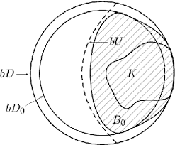
If $\mathrm{a}$ and $\mathrm{b}$ are symmetric with respect to $a$ circle $\mathrm{K}$, then their images $\tilde{\mathrm{a}}$ and $\widetilde{\mathrm{b}}$ under inversion in any circle $\mathrm{J}$ are again symmetric with respect to the image $\widetilde{\mathrm{K}}$ of $\mathrm{K}$.
To understand this, first note that, since inversion is anticonformal, (3.10) is just a special case of the following more general result:
Inversion maps any pair of orthogonal circles to another pair of orthogonal circles.
Of course if one of the circles passes through the centre of inversion then its image will be a line. However, if we think of lines as merely being circles of infinite radius then the result is true without qualification.

The preservation of symmetry result is now easily understood. See [3.11b]. Since the two dashed circles through $\mathrm{a}$ and $\mathrm{b}$ are orthogonal to $\mathrm{K}$, their images under inversion in J are likewise orthogonal to $\widetilde{K}$, and they therefore intersect in a pair of points that are symmetric with respect to $\widetilde{K}$.

数学代写|复分析作业代写Complex function代考|Inversion in a Sphere

Inversion $J_S$ of three-dimensional space in a sphere $\mathrm{S}$ (radius $\mathrm{R}$ and centre $\mathrm{q}$ ) is defined in the obvious way: if $p$ is a point in space at distance $\rho$ from $q$, then $\mathcal{J}_S(p)$ is the point in the same direction from $q$ as $p$, and at distance $\left(R^2 / \rho\right)$ from $q$. We should explain that this is not generalization for its own sake; soon we will see how this three-dimensional inversion sheds new light on two-dimensional inversion in $\mathbb{C}$.

Without any additional work, we may immediately generalize most of the above results on inversion in circles to results on inversion in spheres. For example, reconsider [3.3]. If we rotate this figure (in space) about the line through $q$ and $a$, then we obtain [3.12], in which the circle of inversion $\mathrm{K}$ has swept out a sphere of inversion $S$, and the line has swept out a plane $\Pi$. Thus we have the following result:
Under inversion in a sphere centred at q, a plane $\Pi$ that does not contain $\mathrm{q}$ is mapped to a sphere that contains $\mathrm{q}$ and whose tangent plane there is parallel to $\Pi$. Conversely, a sphere containing $\mathrm{q}$ is mapped to a plane that is parallel to the tangent plane of that sphere at $\mathrm{q}$.

By the same token, if we rotate figure [3.4] about the line through $q$ and $a$, then we find that
Under inversion in a sphere, the image of a sphere that does not contain the centre of inversion is another sphere that does not contain the centre of inversion.
This result immediately tells us what will happen to a circle in space under inversion in a sphere, for such a circle may be thought of as the intersection of two spheres. Thus we easily deduce [exercise] the following result:
Under inversion in a sphere, the image of a circle $\mathrm{C}$ that does not pass through the centre $\mathrm{q}$ of inversion is another circle that does not pass through q. If $\mathrm{C}$ does pass through $\mathrm{q}$ then the image is a line parallel to the tangent of $\mathrm{C}$ at $\mathrm{q}$.
The close connection between inversion in a circle and reflection in a line also persists: reflection in a plane is a limiting case of inversion in a sphere. For this reason, inversion in a sphere is also called “reflection in a sphere”.

复分析代写

数学代写|复分析作业代写Complex function代考|Preservation of Symmetry

考虑 [3.11a]，它显示了两点 $\mathrm{a}$ 和 $\mathrm{b}$ 相对于线 $\mathrm{L}$ 对称。如果线中的反射 $M$ 映射到 $\tilde{a}, b$ 到 $\tilde{b}$ ，和 $L$ 到 $\tilde{L}$ ，然后清 晰的图像点 $\tilde{a}$ 和 $\tilde{b}$ 再次关于图像线对称 $\tilde{L}$. 简而言之，线中的反射相对于线“保持对称性”。
我们现在表明，圆中的反射也保持关于圆的对称性:
如果 $\mathrm{a}$ 和b对称于 $a$ 圆圈K，然后他们的图像 $\mathrm{a}$ 和 $\mathrm{b}$ 在任意圈内反转 $\mathrm{J}$ 再次关于图像对称 $\widetilde{\mathrm{K}}$ 的K.
要理解这一点，首先要注意，由于反演是反共形的，(3.10) 只是以下更一般结果的特例:
反演将任何一对正交圆映射到另一对正交圆。
当然，如果其中一个圆圈穿过反转中心，那么它的图像将是一条线。然而，如果我们将线仅仅看作是无限 半径的圆，那么结果是没有条件的。
对称性保持结果现在很容易理解。见 [3.11b]。由于两个虚线圆圈通过a和b正交于 $K$ ，它们在 」 中反转的 图像同样正交于 $\widetilde{K}$ ，因此它们相交于一对对称于 $\widetilde{K}$.

数学代写|复分析作业代写Complex function代考|Inversion in a Sphere

反转 $J_S$ 球体中的三维空间 $\mathrm{S}$ (半径R和中心q) 以显而易见的方式定义：如果 $p$ 是远处空间中的一个点 $\rho 从 q$ ，然后 $\mathcal{J}_S(p)$ 是同一个方向的点 $q$ 作为 $p$ ，在远处 $\left(R^2 / \rho\right)$ 从 $q$. 我们应该解释这并不是为了泛化而泛化；很 快我们就会看到这个三维反演如何为二维反演提供新的思路 $\mathbb{C}$.
无需任何额外工作，我们可以立即将上述大部分关于圆圈反演的结果推广到球体反演的结果。例如，重新 考虑 [3.3]。如果我们围绕直线旋转这个图形 (在空间中) $q$ 和 $a$ ，然后我们得到 [3.12], 其中反转圆K扫过 一个反转球体 $S$ ，直线扫过一个平面 $\Pi$. 行于该球体切平面的平面q.
出于同样的原因，如果我们围绕穿过的直线旋转图 [3.4] $[$ 和 $a$ ，那么我们发现
在球体反演下，一个不包含反演中心的球体的图像是另一个不包含反演中心的球体。
这个结果立即告诉我们在球面反转下空间中的圆会发生什么，因为这样的圆可以被认为是两个球的交点。
因此我们很容易推导出[练习]以下结果：C不通过中心 $q$ 的反转是另一个不通过 $q$ 的圆。如果C确实通过 $q$ 那么图像是一条平行于切线的线C在q.
圆中的反演与直线中的反射之间的密切联系也依然存在: 平面中的反射是球体中反演的一种极限情况。因 此，球面反转也称为“球面反射”。

统计代写请认准statistics-lab™. statistics-lab™为您的留学生涯保驾护航。

金融工程代写

金融工程是使用数学技术来解决金融问题。金融工程使用计算机科学、统计学、经济学和应用数学领域的工具和知识来解决当前的金融问题，以及设计新的和创新的金融产品。

非参数统计代写

非参数统计指的是一种统计方法，其中不假设数据来自于由少数参数决定的规定模型；这种模型的例子包括正态分布模型和线性回归模型。

广义线性模型代考

广义线性模型（GLM）归属统计学领域，是一种应用灵活的线性回归模型。该模型允许因变量的偏差分布有除了正态分布之外的其它分布。

术语 广义线性模型（GLM）通常是指给定连续和/或分类预测因素的连续响应变量的常规线性回归模型。它包括多元线性回归，以及方差分析和方差分析（仅含固定效应）。

有限元方法代写

有限元方法（FEM）是一种流行的方法，用于数值解决工程和数学建模中出现的微分方程。典型的问题领域包括结构分析、传热、流体流动、质量运输和电磁势等传统领域。

有限元是一种通用的数值方法，用于解决两个或三个空间变量的偏微分方程（即一些边界值问题）。为了解决一个问题，有限元将一个大系统细分为更小、更简单的部分，称为有限元。这是通过在空间维度上的特定空间离散化来实现的，它是通过构建对象的网格来实现的：用于求解的数值域，它有有限数量的点。边界值问题的有限元方法表述最终导致一个代数方程组。该方法在域上对未知函数进行逼近。[1] 然后将模拟这些有限元的简单方程组合成一个更大的方程系统，以模拟整个问题。然后，有限元通过变化微积分使相关的误差函数最小化来逼近一个解决方案。

tatistics-lab作为专业的留学生服务机构，多年来已为美国、英国、加拿大、澳洲等留学热门地的学生提供专业的学术服务，包括但不限于Essay代写，Assignment代写，Dissertation代写，Report代写，小组作业代写，Proposal代写，Paper代写，Presentation代写，计算机作业代写，论文修改和润色，网课代做，exam代考等等。写作范围涵盖高中，本科，研究生等海外留学全阶段，辐射金融，经济学，会计学，审计学，管理学等全球99%专业科目。写作团队既有专业英语母语作者，也有海外名校硕博留学生，每位写作老师都拥有过硬的语言能力，专业的学科背景和学术写作经验。我们承诺100%原创，100%专业，100%准时，100%满意。

随机分析代写

随机微积分是数学的一个分支，对随机过程进行操作。它允许为随机过程的积分定义一个关于随机过程的一致的积分理论。这个领域是由日本数学家伊藤清在第二次世界大战期间创建并开始的。

时间序列分析代写

随机过程，是依赖于参数的一组随机变量的全体，参数通常是时间。 随机变量是随机现象的数量表现，其时间序列是一组按照时间发生先后顺序进行排列的数据点序列。通常一组时间序列的时间间隔为一恒定值（如1秒，5分钟，12小时，7天，1年），因此时间序列可以作为离散时间数据进行分析处理。研究时间序列数据的意义在于现实中，往往需要研究某个事物其随时间发展变化的规律。这就需要通过研究该事物过去发展的历史记录，以得到其自身发展的规律。

回归分析代写

多元回归分析渐进（Multiple Regression Analysis Asymptotics）属于计量经济学领域，主要是一种数学上的统计分析方法，可以分析复杂情况下各影响因素的数学关系，在自然科学、社会和经济学等多个领域内应用广泛。

MATLAB代写

MATLAB 是一种用于技术计算的高性能语言。它将计算、可视化和编程集成在一个易于使用的环境中，其中问题和解决方案以熟悉的数学符号表示。典型用途包括：数学和计算算法开发建模、仿真和原型制作数据分析、探索和可视化科学和工程图形应用程序开发，包括图形用户界面构建MATLAB 是一个交互式系统，其基本数据元素是一个不需要维度的数组。这使您可以解决许多技术计算问题，尤其是那些具有矩阵和向量公式的问题，而只需用 C 或 Fortran 等标量非交互式语言编写程序所需的时间的一小部分。MATLAB 名称代表矩阵实验室。MATLAB 最初的编写目的是提供对由 LINPACK 和 EISPACK 项目开发的矩阵软件的轻松访问，这两个项目共同代表了矩阵计算软件的最新技术。MATLAB 经过多年的发展，得到了许多用户的投入。在大学环境中，它是数学、工程和科学入门和高级课程的标准教学工具。在工业领域，MATLAB 是高效研究、开发和分析的首选工具。MATLAB 具有一系列称为工具箱的特定于应用程序的解决方案。对于大多数 MATLAB 用户来说非常重要，工具箱允许您学习和应用专业技术。工具箱是 MATLAB 函数（M 文件）的综合集合，可扩展 MATLAB 环境以解决特定类别的问题。可用工具箱的领域包括信号处理、控制系统、神经网络、模糊逻辑、小波、仿真等。

R语言代写	问卷设计与分析代写
PYTHON代写	回归分析与线性模型代写
MATLAB代写	方差分析与试验设计代写
STATA代写	机器学习/统计学习代写
SPSS代写	计量经济学代写
EVIEWS代写	时间序列分析代写
EXCEL代写	深度学习代写
SQL代写	各种数据建模与可视化代写

如果你也在 怎样代写复分析Complex function这个学科遇到相关的难题，请随时右上角联系我们的24/7代写客服。

复分析是一个从复数到复数的函数。换句话说，它是一个以复数的一个子集为域，以复数为子域的函数。复数函数通常应该有一个包含复数平面的非空开放子集的域。

statistics-lab™ 为您的留学生涯保驾护航 在代写复分析Complex function方面已经树立了自己的口碑, 保证靠谱, 高质且原创的统计Statistics代写服务。我们的专家在代写复分析Complex function代写方面经验极为丰富，各种代写复分析Complex function相关的作业也就用不着说。

我们提供的复分析Complex function及其相关学科的代写，服务范围广, 其中包括但不限于:

• Statistical Inference 统计推断
• Statistical Computing 统计计算
• Advanced Probability Theory 高等概率论
• Advanced Mathematical Statistics 高等数理统计学
• (Generalized) Linear Models 广义线性模型
• Statistical Machine Learning 统计机器学习
• Longitudinal Data Analysis 纵向数据分析
• Foundations of Data Science 数据科学基础

数学代写|复分析作业代写Complex function代考|Preservation of Circles

Let us examine the effect of $\mathfrak{I}_K$ on lines and then on circles. If a line $L$ passes through the centre $q$ of $K$, then clearly $J_K$ maps $L$ to itself, which we may write as $\mathcal{I}_K(L)=L$. Of course we don’t mean that each point of $L$ remains fixed, for $I_K$ interchanges the portions of $L$ interior and exterior to $K$; the only points of $L$ that remain fixed are the two places where it intersects $\mathrm{K}$.

Matters become much more interesting when we consider a general line $\mathrm{L}$ that does not pass through q. Figure [3.3] provides the surprising answer:
If a line $\mathrm{L}$ does not pass through the centre $\mathrm{q}$ of $\mathrm{K}$, then inversion in $\mathrm{K}$ maps $\mathrm{L}$ to a circle that passes through $\mathrm{q}$.
Here $b$ is an arbitrary point on $L$, while $a$ is the intersection of $L$ with the perpendicular line through q. By virtue of (3.5), $\angle \mathbf{q} \widetilde{\mathbf{a}} \widetilde{\mathrm{a}}=\angle \mathrm{qab}=(\pi / 2)$, so $\widetilde{\mathrm{b}}$ lies on the circle having the line-segment $q \tilde{a}$ as diameter. Done. Notice, incidentally, that the tangent at $q$ of the image circle is parallel to $L$.

Note that (3.7) makes no mention of the radius R of K. You may therefore be concerned that in [3.3] we have chosen $\mathrm{R}$ so that $\mathrm{K}$ does not intersect $\mathrm{L}$; what happens if $\mathrm{K}$ does intersect $\mathrm{L}$ ? Check for yourself that, while the picture looks somewhat different in this case, the geometric argument above continues to apply without any modification.

We now give a less direct, but more instructive way of understanding why (3.7) does not depend on the size of $\mathrm{K}$. We will show that if the result holds for one circle $K_1$ (radius $R_1$ ) centred at $q$, then it will hold for any other circle $K_2$ (radius $R_2$ ) centred at $q$.

Let $z$ be an arbitrary point, and let $\widetilde{z}1=\mathcal{J}{K_1}(z)$ and $\widetilde{z}2=\mathcal{J}{K_2}(z)$. Obviously $\widetilde{z}1$ and $\tilde{z}_2$ are both in the same direction from $q$ as $z$, and you can easily check that the ratio of their distances from $\mathrm{q}$ is independent of the location of $\mathrm{z}$ : $$ \left[q \tilde{z}_2\right] /\left[q \tilde{z}_1\right]=\left(R_2 / R_1\right)^2 \equiv \mathrm{k} \text {, say. } $$ Thus $$ \mathcal{J}{K_2}=\mathcal{D}{\mathrm{q}}^k \circ \mathcal{J}{\mathrm{K}1}, $$ where the “central dilation” $\mathcal{D}{\mathrm{q}}^k$ [see p. 45] is an expansion (centred at q) of the plane by a factor of $k$. It follows [exercise] that if (3.7) holds for $K_1$ then it also holds for $K_2$.

数学代写|复分析作业代写Complex function代考|Preservation of Angles

Let us begin by discussing what is meant by “preservation of angles”. In the centre of [3.8] are two curves $S_1$ and $S_2$ intersecting at a point $p$. Provided these curves are sufficiently smooth at $p$, then, as illustrated, we may draw their tangent lines $\mathrm{T}_1$ and $T_2$ at $p$. We now define the “angle between $S_1$ and $S_2$ ” at $p$ to be the acute angle $\theta$ from $T_1$ to $T_2$. Thus this angle $\theta$ has a sign attached to it: the angle between $S_2$ and $S_1$ is minus the illustrated angle between $\mathrm{S}_1$ and $\mathrm{S}_2$. If we now apply a sufficiently smooth transformation to the curves, then the image curves will again possess tangents at the image of $p$, and so there will be a well-defined angle between these image curves.

If the angle between the image curves is the same as the angle between the original curves through $\mathrm{p}$, then we say that the transformation has “preserved” the angle at $p$. It is perfectly possible that the transformation preserves the angle between one pair of curves through $p$, but not every pair through $p$. However, if the transformation does preserve the angle between every pair of curves through $\mathrm{p}$, then we say that it is conformal at $p$. We stress that this means that both the magnitude and the sign of the angles are preserved; see the right of [3.8]. If every angle at $p$ is instead mapped to an angle of equal magnitude but opposite sign, then we say that the mapping is anticonformal at p; see the left of [3.8]. If the mapping is conformal at every point in the region where it is defined, then we call it a conformal mapping; if it is instead anticonformal at every point, then we call it an anticonformal mapping. Finally, if a mapping is known to preserve the magnitude of angles, but we are unable to say whether or not it preserves their sense, then we call it an isogonal mapping.

复分析代写

数学代写|复分析作业代写Complex function代考|Preservation of Circles

让我们检查一下效果 $J_K$ 在线上，然后在圆圈上。如果一条线 $L$ 穿过中心 $q$ 的 $K$ ，那么很明显 $J_K$ 地图 $L$ 对它 自己，我们可以写成 $\mathcal{I}_K(L)=L$. 当然我们并不是说每一点 $L$ 保持不变，因为 $I_K$ 互换的部分 $L$ 内部和外 部 $K ;$ 唯一的要点 $L$ 保持固定的是它相交的两个地方 $K$.
当我们考虑一条总路线时，事情就变得有趣多了L不通过 q。图 [3.3] 提供了令人惊讶的答案: 如果一条线L不通过中心q的K， 然后反演K地图L到一个穿过的圆q.
这里 $b$ 是一个任意点 $L$ ，尽管 $a$ 是交集 $L$ 与通过 $q$ 的垂直线。凭借 (3.5)， $\angle \mathbf{q a ̃} \tilde{a}=\angle \mathrm{qab}=(\pi / 2)$ ，所 以 $\tilde{b}$ 位于具有线段的圆上 $q \tilde{a}$ 作为直径。完毕。顺便注意，切线位于 $q$ 像圈的平行于 $L$.
注意 (3.7) 没有提到 $K$ 的半径 $R$ 。因此你可能会担心在 [3.3] 中我们选择了 $\mathrm{R}$ 以便 $K$ 不相交 $L$; 如果会发生 什么K相交L? 自己检查一下，虽然在这种情况下图片看起来有些不同，但上面的几何论证继续适用而无 需任何修改。
我们现在给出一种不太直接但更有启发性的方式来理解为什么 (3.7) 不依赖于 $\mathrm{K}$. 我们将证明，如果结果适
让 $z$ 是一个任意点，让 $\tilde{z} 1=\mathcal{J} K_1(z)$ 和 $\tilde{z} 2=\mathcal{J} K_2(z)$. 明显地 $\tilde{z} 1$ 和 $\tilde{z}_2$ 都在同一个方向 $q$ 作为 $z$ ，你可 以很容易地检查它们与 $q$ 与位置无关z :
$$
\left[q \tilde{z}_2\right] /\left[q \tilde{z}_1\right]=\left(R_2 / R_1\right)^2 \equiv \mathrm{k}, \text { say }
$$
因此
$$
\mathcal{J} K_2=\mathcal{D} \mathrm{q}^k \circ \mathcal{J} K 1
$$
“中心扩张”在哪里 $\mathcal{D} \mathrm{q}^k$ [见第 45] 是平面的扩展 (以 q 为中心) $k$. 它遵循 [练习] 如果 (3.7) 成立 $K_1$ 那么它 也适用于 $K_2$.

数学代写|复分析作业代写Complex function代考|Preservation of Angles

让我们首先讨论“角度保持”的含义。[3.8] 的中心是两条曲线小号1和小号2相交于一点p. 只要这些曲线在p，然后，如图所示，我们可以画出它们的切线吨1和吨2在p. 我们现在定义“之间的角度小号1和小号2“ 在p是锐角我从吨1到吨2. 因此这个角度我附有一个标志：之间的角度小号2和小号1减去图示的夹角小号1和小号2. 如果我们现在对曲线应用足够平滑的变换，那么图像曲线将再次在图像处具有切线p, 因此这些图像曲线之间将有一个明确定义的角度。

如果图像曲线之间的角度与原始曲线之间的角度相同p，然后我们说变换“保留”了角度p. 完全有可能变换保留一对曲线之间的角度p，但不是每一对通过p. 但是，如果变换确实保留了每对曲线之间的角度p, 那么我们说它是共形的p. 我们强调这意味着角度的大小和符号都被保留；见[3.8]右边。如果每个角度都在p相反映射到大小相等但符号相反的角度，那么我们说映射在 p 处是反共形的；见[3.8]的左边。如果映射在它定义的区域中的每个点都是共形的，那么我们称它为共形映射；如果它在每一点都是反共形的，那么我们称它为反共形映射。最后，如果已知映射可以保持角度的大小，但我们无法说它是否保持角度的意义，那么我们称它为等角映射。

统计代写请认准statistics-lab™. statistics-lab™为您的留学生涯保驾护航。

金融工程代写

金融工程是使用数学技术来解决金融问题。金融工程使用计算机科学、统计学、经济学和应用数学领域的工具和知识来解决当前的金融问题，以及设计新的和创新的金融产品。

非参数统计代写

非参数统计指的是一种统计方法，其中不假设数据来自于由少数参数决定的规定模型；这种模型的例子包括正态分布模型和线性回归模型。

广义线性模型代考

广义线性模型（GLM）归属统计学领域，是一种应用灵活的线性回归模型。该模型允许因变量的偏差分布有除了正态分布之外的其它分布。

术语 广义线性模型（GLM）通常是指给定连续和/或分类预测因素的连续响应变量的常规线性回归模型。它包括多元线性回归，以及方差分析和方差分析（仅含固定效应）。

有限元方法代写

有限元方法（FEM）是一种流行的方法，用于数值解决工程和数学建模中出现的微分方程。典型的问题领域包括结构分析、传热、流体流动、质量运输和电磁势等传统领域。

有限元是一种通用的数值方法，用于解决两个或三个空间变量的偏微分方程（即一些边界值问题）。为了解决一个问题，有限元将一个大系统细分为更小、更简单的部分，称为有限元。这是通过在空间维度上的特定空间离散化来实现的，它是通过构建对象的网格来实现的：用于求解的数值域，它有有限数量的点。边界值问题的有限元方法表述最终导致一个代数方程组。该方法在域上对未知函数进行逼近。[1] 然后将模拟这些有限元的简单方程组合成一个更大的方程系统，以模拟整个问题。然后，有限元通过变化微积分使相关的误差函数最小化来逼近一个解决方案。

tatistics-lab作为专业的留学生服务机构，多年来已为美国、英国、加拿大、澳洲等留学热门地的学生提供专业的学术服务，包括但不限于Essay代写，Assignment代写，Dissertation代写，Report代写，小组作业代写，Proposal代写，Paper代写，Presentation代写，计算机作业代写，论文修改和润色，网课代做，exam代考等等。写作范围涵盖高中，本科，研究生等海外留学全阶段，辐射金融，经济学，会计学，审计学，管理学等全球99%专业科目。写作团队既有专业英语母语作者，也有海外名校硕博留学生，每位写作老师都拥有过硬的语言能力，专业的学科背景和学术写作经验。我们承诺100%原创，100%专业，100%准时，100%满意。

随机分析代写

随机微积分是数学的一个分支，对随机过程进行操作。它允许为随机过程的积分定义一个关于随机过程的一致的积分理论。这个领域是由日本数学家伊藤清在第二次世界大战期间创建并开始的。

时间序列分析代写

随机过程，是依赖于参数的一组随机变量的全体，参数通常是时间。 随机变量是随机现象的数量表现，其时间序列是一组按照时间发生先后顺序进行排列的数据点序列。通常一组时间序列的时间间隔为一恒定值（如1秒，5分钟，12小时，7天，1年），因此时间序列可以作为离散时间数据进行分析处理。研究时间序列数据的意义在于现实中，往往需要研究某个事物其随时间发展变化的规律。这就需要通过研究该事物过去发展的历史记录，以得到其自身发展的规律。

回归分析代写

多元回归分析渐进（Multiple Regression Analysis Asymptotics）属于计量经济学领域，主要是一种数学上的统计分析方法，可以分析复杂情况下各影响因素的数学关系，在自然科学、社会和经济学等多个领域内应用广泛。

MATLAB代写

MATLAB 是一种用于技术计算的高性能语言。它将计算、可视化和编程集成在一个易于使用的环境中，其中问题和解决方案以熟悉的数学符号表示。典型用途包括：数学和计算算法开发建模、仿真和原型制作数据分析、探索和可视化科学和工程图形应用程序开发，包括图形用户界面构建MATLAB 是一个交互式系统，其基本数据元素是一个不需要维度的数组。这使您可以解决许多技术计算问题，尤其是那些具有矩阵和向量公式的问题，而只需用 C 或 Fortran 等标量非交互式语言编写程序所需的时间的一小部分。MATLAB 名称代表矩阵实验室。MATLAB 最初的编写目的是提供对由 LINPACK 和 EISPACK 项目开发的矩阵软件的轻松访问，这两个项目共同代表了矩阵计算软件的最新技术。MATLAB 经过多年的发展，得到了许多用户的投入。在大学环境中，它是数学、工程和科学入门和高级课程的标准教学工具。在工业领域，MATLAB 是高效研究、开发和分析的首选工具。MATLAB 具有一系列称为工具箱的特定于应用程序的解决方案。对于大多数 MATLAB 用户来说非常重要，工具箱允许您学习和应用专业技术。工具箱是 MATLAB 函数（M 文件）的综合集合，可扩展 MATLAB 环境以解决特定类别的问题。可用工具箱的领域包括信号处理、控制系统、神经网络、模糊逻辑、小波、仿真等。

R语言代写	问卷设计与分析代写
PYTHON代写	回归分析与线性模型代写
MATLAB代写	方差分析与试验设计代写
STATA代写	机器学习/统计学习代写
SPSS代写	计量经济学代写
EVIEWS代写	时间序列分析代写
EXCEL代写	深度学习代写
SQL代写	各种数据建模与可视化代写

如果你也在 怎样代写复分析Complex function这个学科遇到相关的难题，请随时右上角联系我们的24/7代写客服。

复分析是一个从复数到复数的函数。换句话说，它是一个以复数的一个子集为域，以复数为子域的函数。复数函数通常应该有一个包含复数平面的非空开放子集的域。

statistics-lab™ 为您的留学生涯保驾护航 在代写复分析Complex function方面已经树立了自己的口碑, 保证靠谱, 高质且原创的统计Statistics代写服务。我们的专家在代写复分析Complex function代写方面经验极为丰富，各种代写复分析Complex function相关的作业也就用不着说。

我们提供的复分析Complex function及其相关学科的代写，服务范围广, 其中包括但不限于:

• Statistical Inference 统计推断
• Statistical Computing 统计计算
• Advanced Probability Theory 高等概率论
• Advanced Mathematical Statistics 高等数理统计学
• (Generalized) Linear Models 广义线性模型
• Statistical Machine Learning 统计机器学习
• Longitudinal Data Analysis 纵向数据分析
• Foundations of Data Science 数据科学基础

数学代写|复分析作业代写Complex function代考|Approximating a Power Series with a Polynomial

Implicit in the definition of convergence is a simple but very important fact: if $P(a)$ converges, then its value can be approximated by the partial sum $\mathrm{P}{\mathrm{m}}(\mathrm{a})$, and by choosing a sufficiently large value of $m$ we can make the approximation as accurate as we wish. Combining this observation with (2.11), At each point $\mathrm{z}$ in the disc of convergence, $\mathrm{P}(\mathrm{z})$ can be approximated with arbitrarily high precision by a polynomial $\mathrm{P}{\mathrm{m}}(\mathrm{z})$ of sufficiently high degree.
For simplicity’s sake, let us investigate this further in the case that $P(z)$ is centred at the origin. The error $E_m(z)$ at $z$ associated with the approximation $P_m(z)$ can be defined as the distance $E_m(z)=\left|P(z)-P_m(z)\right|$ between the exact answer and the approximation. For a fixed value of $m$, the error $E_m(z)$ will vary as $z$ moves around in the disc of convergence. Clearly, since $E_m(0)=0$, the error will be extremely small if $z$ is close to the origin, but what if $z$ approaches the circle of convergence? The answer depends on the particular power series, but it can happen that the error becomes enormous! [See Ex. 12.] This does not contradict the above result: for any fixed $z$, no matter how close to the circle of convergence, the error $\mathrm{E}_m(z)$ will become arbitrarily small as $m$ tends to infinity.

This problem is avoided if we restrict $z$ to the disc $|z| \leqslant r$, where $r<R$, because this prevents $z$ from getting arbitrarily close to the circle of convergence, $|z|=R$. In attempting to approximate $P(z)$ within this disc, it turns out that we can do the following. We first decide on the maximum error (say $\epsilon$ ) that we are willing to put up with, then choose (once and for all) an approximating polynomial $\mathrm{P}_{\mathrm{m}}(z)$ of sufficiently high degree that the error is smaller than $\epsilon$ throughout the disc. That is, throughout the disc, the approximating point $P_m(z)$ lies less than $\epsilon$ away from the true point, $\mathrm{P}(z)$. One describes this by saying that $\mathrm{P}(z)$ is uniformly convergent on this disc:
If $\mathrm{P}(z)$ has disc of convergence $|z|<\mathrm{R}$, then $\mathrm{P}(z)$ is uniformly convergent on the closed disc $|z| \leqslant r$, where $r<R$.
Although we may not have uniform convergence on the whole disc of convergence, the above result shows that this is really a technicality: we do have uniform convergence on a disc that almost fills the complete disc of convergence, say $\mathrm{r}=(0.999999999) \mathrm{R}$.
To verify (2.12), first do Ex. 12, then have a good look at (2.9).

数学代写|复分析作业代写Complex function代考|Uniqueness

If a complex function can be expressed as a power series, then it can only be done so in one way-the power series is unique. This is an immediate consequence of the Identity Theorem:
If
$$
\mathrm{c}0+\mathrm{c}_1 z+\mathrm{c}_2 z^2+\mathrm{c}_3 z^3+\cdots=\mathrm{d}_0+\mathrm{d}_1 z+\mathrm{d}_2 z^2+\mathrm{d}_3 z^3+\cdots $$ for all $z$ in a neighbourhood (no matter how small) of 0 , then the power series are identical: $\mathrm{c}{\mathrm{j}}=\mathrm{d}_{\mathbf{j}}$.
Putting $z=0$ yields $c_0=\mathrm{d}_0$, so they may be cancelled from both sides. Dividing by $z$ and again putting $z=0$ then yields $c_1=d_1$, and so on. [Although this was easy, Ex. 13 shows that it is actually rather remarkable.] The result can be strengthened considerably: If the power series merely agree along a segment of curve (no matter how small) through 0, or if they agree at every point of an infinite sequence of points that converges to 0, then the series are identical. The verification is essentially the same, only instead of putting $z=0$, we now take the limit as $z$ approaches 0 , either along the segment of curve or through the sequence of points.

We can perhaps make greater intuitive sense of these results if we first recall that a power series can be approximated with arbitrarily high precision by a polynomial of sufficiently high degree. Given two points in the plane (no matter how close together) there is a unique line passing through them. Thinking in terms of a graph $y=f(x)$, this says that a polynomial of degree 1 , say $f(x)=c_0+c_1 x$, is uniquely determined by the images of any two points, no matter how close together. Likewise, in the case of degree 2, if we are given three points (no matter how close together), there is only one parabolic graph $y=f(x)=c_0+c_1 x+c_2 x^2$ that can be threaded through them. This idea easily extends to complex functions: there is one, and only one, complex polynomial of degree $n$ that maps a given set of $(n+1)$ points to a given set of $(n+1)$ image points. The above result may therefore be thought of as the limiting case in which the number of known points (together with their known image points) tends to infinity.

Earlier we alluded to a sense in which $h(z)=1 /\left(1+z^2\right)$ is the only complex function that agrees with the real function $H(x)=1 /\left(1+x^2\right)$ on the real line. Yet clearly we can easily write down infinitely many complex functions that agree with $\mathrm{H}(x)$ in this way. For example,
$$
g(z)=g(x+i y)=\frac{\cos \left[x^2 y\right]+i \sin \left[y^2\right]}{e^y+x^2 \ln \left(e+y^4\right)}
$$
Then in what sense can $h(z)$ be considered the unique generalization of $\mathrm{H}(\mathrm{x})$ ?
We already know that $h(z)$ can be expressed as the power series $\sum_{j=0}^{\infty}(-1)^j z^{2 j}$, and this fact yields [exercise] a provisional answer: $h(z)$ is the only complex function that (i) agrees with $\mathrm{H}(\mathrm{x})$ on the real axis, and (ii) can be expressed as a power series in $z$. This still does not completely capture the sense in which $h(z)$ is unique, but it’s a start.

复分析代写

数学代写|复分析作业代写Complex function代考|Approximating a Power Series with a Polynomial

收敛定义中隐含了一个简单但非常重要的事实: 如果 $P(a)$ 收敛，那么它的值可以用部分和来近似 $\operatorname{Pm}(\mathrm{a})$ ，并通过选择足够大的值 $m$ 我们可以使近似值尽可能准确。将此观察结果与 (2.11) 相结合，在 每个点 $z$ 在会聚圆盘中， $\mathrm{P}(\mathrm{z})$ 可以通过多项式以任意高精度近似 $\operatorname{Pm}(\mathrm{z})$ 足够高的程度。
为了简单起见，让我们在以下情况下进一步调查 $P(z)$ 以原点为中心。错误 $E_m(z)$ 在 $z$ 与近似相关 $P_m(z)$ 可以定义为距离 $E_m(z)=\left|P(z)-P_m(z)\right|$ 在准确答案和近似值之间。对于固定值 $m$ ，错误 $E_m(z)$ 会有所不同 $z$ 在会聚圆盘中四处移动。显然，因为 $E_m(0)=0$, 如果 $z$ 接近原点，但如果 $z$ 接近收 敛圆? 答案取决于特定的帋级数，但误差可能会变得很大! [见例。12.] 这与上述结果并不矛盾：对于任 何固定的 $z$ ，无论收敛圆有多接近，误差 $\mathrm{E}m(z)$ 将变得任意小 $m$ 趋于无穷大。 如果我们限制这个问题就可以避免 $z$ 到光盘 $|z| \leqslant r$ ，在哪里 $r{\mathrm{m}}(z)$ 程度足够高，误差小于 $\epsilon$ 整个 光盘。即，在整个圆盘中，逼近点 $P_m(z)$ 小于 $\epsilon$ 远离真实点， $\mathrm{P}(z)$.一个人这样描述这个 $\mathrm{P}(z)$ 在这个圆 盘上一致收敛:
如果 $\mathrm{P}(z)$ 有收敛圆盘 $|z|<\mathrm{R}$ ，然后 $\mathrm{P}(z)$ 一致收敛于闭盘 $|z| \leqslant r$ ，在哪里 $r<R$.
虽然我们可能没有在整个收敛圆盘上一致收敛，但上面的结果表明这确实是一个技术问题: 我们在几乎 填满整个收敛圆盘的圆盘上确实有一致收敛，比如说 $r=(0.999999999) R$. 要验证 (2.12)，首先做 Ex. 12，然后好好看看（2.9）。

数学代写|复分析作业代写Complex function代考|Uniqueness

如果一个复杂的函数可以表示为幂级数，那么只能用一种方式来表示一一幂级数是唯一的。这是恒等定 理的直接结果： 如果
$$
\mathrm{c} 0+\mathrm{c}1 z+\mathrm{c}_2 z^2+\mathrm{c}_3 z^3+\cdots=\mathrm{d}_0+\mathrm{d}_1 z+\mathrm{d}_2 z^2+\mathrm{d}_3 z^3+\cdots $$ 对全部 $z$ 在 0 的邻域 (无论多小) 中，幂级数相同： $c j=\mathrm{d}{\mathbf{j}}$.
推杆 $z=0$ 产量 $c_0=\mathrm{d}0$ ，所以他们可能会从双方取消。除以 $z$ 再次投入 $z=0$ 然后产量 $c_1=d_1$ ，等 等。[虽然这很容易，Ex。13 表明它实际上相当显着。] 结果可以大大加强：如果幂级数仅沿着通过 0 的 曲线段 (无论多小) 一致，或者如果它们在无限点序列的每个点都一致收敛于0，则级数相同。验证本质 上是一样的，只是代替了put $z=0$ ，我们现在将极限作为 $z$ 沿着曲线段或通过点序列接近 0 。 如果我们首先回忆起可以通过足够高次数的多项式以任意高精度逼近幂级数，我们或许可以更直观地理 解这些结果。给定平面上的两个点（无论距离多近），有一条唯一的线穿过它们。用图表思考 $y=f(x)$ 同样，在 2 次的情况下，如果给我们三个点（无论多近），则只有一个抛物线图 $y=f(x)=c_0+c_1 x+c_2 x^2$ 可以穿过它们。这个想法很容易扩展到复杂的功能：有一个，而且只有 一个，复杂的次数多项式 $n$ 映射一组给定的 $(n+1)$ 指向一组给定的 $(n+1)$ 图像点。因此，上述结果可 以被认为是已知点 (连同它们的已知图像点) 的数量趋于无穷大的极限情况。 早些时候我们提到了一种感觉 $h(z)=1 /\left(1+z^2\right)$ 是唯一符合实函数的复函数 $H(x)=1 /\left(1+x^2\right)$ 在实线上。然而很明显，我们可以很容易地写出无限多的复杂函数，这些函数符合 $\mathrm{H}(x)$ 这样。例如， $$ g(z)=g(x+i y)=\frac{\cos \left[x^2 y\right]+i \sin \left[y^2\right]}{e^y+x^2 \ln \left(e+y^4\right)} $$ 那么在什么意义上可以 $h(z)$ 被认为是 $\mathrm{H}(\mathrm{x}) ?$ 我们已经知道 $h(z)$ 可以表示为幂级数 $\sum{j=0}^{\infty}(-1)^j z^{2 j}$ ，这个事实产生了[练习]一个临时的答案: $h(z)$ 是 (i) 同意的唯一复杂函数 $\mathrm{H}(\mathrm{x}$ ) 在实轴上，并且 (ii) 可以表示为幂级数 $z$. 这仍然没有完全捕捉到 $h(z)$ 是独一无二的，但这是一个开始。

统计代写请认准statistics-lab™. statistics-lab™为您的留学生涯保驾护航。

金融工程代写

金融工程是使用数学技术来解决金融问题。金融工程使用计算机科学、统计学、经济学和应用数学领域的工具和知识来解决当前的金融问题，以及设计新的和创新的金融产品。

非参数统计代写

非参数统计指的是一种统计方法，其中不假设数据来自于由少数参数决定的规定模型；这种模型的例子包括正态分布模型和线性回归模型。

广义线性模型代考

广义线性模型（GLM）归属统计学领域，是一种应用灵活的线性回归模型。该模型允许因变量的偏差分布有除了正态分布之外的其它分布。

术语 广义线性模型（GLM）通常是指给定连续和/或分类预测因素的连续响应变量的常规线性回归模型。它包括多元线性回归，以及方差分析和方差分析（仅含固定效应）。

有限元方法代写

有限元方法（FEM）是一种流行的方法，用于数值解决工程和数学建模中出现的微分方程。典型的问题领域包括结构分析、传热、流体流动、质量运输和电磁势等传统领域。

有限元是一种通用的数值方法，用于解决两个或三个空间变量的偏微分方程（即一些边界值问题）。为了解决一个问题，有限元将一个大系统细分为更小、更简单的部分，称为有限元。这是通过在空间维度上的特定空间离散化来实现的，它是通过构建对象的网格来实现的：用于求解的数值域，它有有限数量的点。边界值问题的有限元方法表述最终导致一个代数方程组。该方法在域上对未知函数进行逼近。[1] 然后将模拟这些有限元的简单方程组合成一个更大的方程系统，以模拟整个问题。然后，有限元通过变化微积分使相关的误差函数最小化来逼近一个解决方案。

tatistics-lab作为专业的留学生服务机构，多年来已为美国、英国、加拿大、澳洲等留学热门地的学生提供专业的学术服务，包括但不限于Essay代写，Assignment代写，Dissertation代写，Report代写，小组作业代写，Proposal代写，Paper代写，Presentation代写，计算机作业代写，论文修改和润色，网课代做，exam代考等等。写作范围涵盖高中，本科，研究生等海外留学全阶段，辐射金融，经济学，会计学，审计学，管理学等全球99%专业科目。写作团队既有专业英语母语作者，也有海外名校硕博留学生，每位写作老师都拥有过硬的语言能力，专业的学科背景和学术写作经验。我们承诺100%原创，100%专业，100%准时，100%满意。

随机分析代写

随机微积分是数学的一个分支，对随机过程进行操作。它允许为随机过程的积分定义一个关于随机过程的一致的积分理论。这个领域是由日本数学家伊藤清在第二次世界大战期间创建并开始的。

时间序列分析代写

随机过程，是依赖于参数的一组随机变量的全体，参数通常是时间。 随机变量是随机现象的数量表现，其时间序列是一组按照时间发生先后顺序进行排列的数据点序列。通常一组时间序列的时间间隔为一恒定值（如1秒，5分钟，12小时，7天，1年），因此时间序列可以作为离散时间数据进行分析处理。研究时间序列数据的意义在于现实中，往往需要研究某个事物其随时间发展变化的规律。这就需要通过研究该事物过去发展的历史记录，以得到其自身发展的规律。

回归分析代写

多元回归分析渐进（Multiple Regression Analysis Asymptotics）属于计量经济学领域，主要是一种数学上的统计分析方法，可以分析复杂情况下各影响因素的数学关系，在自然科学、社会和经济学等多个领域内应用广泛。

MATLAB代写

MATLAB 是一种用于技术计算的高性能语言。它将计算、可视化和编程集成在一个易于使用的环境中，其中问题和解决方案以熟悉的数学符号表示。典型用途包括：数学和计算算法开发建模、仿真和原型制作数据分析、探索和可视化科学和工程图形应用程序开发，包括图形用户界面构建MATLAB 是一个交互式系统，其基本数据元素是一个不需要维度的数组。这使您可以解决许多技术计算问题，尤其是那些具有矩阵和向量公式的问题，而只需用 C 或 Fortran 等标量非交互式语言编写程序所需的时间的一小部分。MATLAB 名称代表矩阵实验室。MATLAB 最初的编写目的是提供对由 LINPACK 和 EISPACK 项目开发的矩阵软件的轻松访问，这两个项目共同代表了矩阵计算软件的最新技术。MATLAB 经过多年的发展，得到了许多用户的投入。在大学环境中，它是数学、工程和科学入门和高级课程的标准教学工具。在工业领域，MATLAB 是高效研究、开发和分析的首选工具。MATLAB 具有一系列称为工具箱的特定于应用程序的解决方案。对于大多数 MATLAB 用户来说非常重要，工具箱允许您学习和应用专业技术。工具箱是 MATLAB 函数（M 文件）的综合集合，可扩展 MATLAB 环境以解决特定类别的问题。可用工具箱的领域包括信号处理、控制系统、神经网络、模糊逻辑、小波、仿真等。

R语言代写	问卷设计与分析代写
PYTHON代写	回归分析与线性模型代写
MATLAB代写	方差分析与试验设计代写
STATA代写	机器学习/统计学习代写
SPSS代写	计量经济学代写
EVIEWS代写	时间序列分析代写
EXCEL代写	深度学习代写
SQL代写	各种数据建模与可视化代写

如果你也在 怎样代写复分析Complex function这个学科遇到相关的难题，请随时右上角联系我们的24/7代写客服。

复分析是一个从复数到复数的函数。换句话说，它是一个以复数的一个子集为域，以复数为子域的函数。复数函数通常应该有一个包含复数平面的非空开放子集的域。

statistics-lab™ 为您的留学生涯保驾护航 在代写复分析Complex function方面已经树立了自己的口碑, 保证靠谱, 高质且原创的统计Statistics代写服务。我们的专家在代写复分析Complex function代写方面经验极为丰富，各种代写复分析Complex function相关的作业也就用不着说。

我们提供的复分析Complex function及其相关学科的代写，服务范围广, 其中包括但不限于:

• Statistical Inference 统计推断
• Statistical Computing 统计计算
• Advanced Probability Theory 高等概率论
• Advanced Mathematical Statistics 高等数理统计学
• (Generalized) Linear Models 广义线性模型
• Statistical Machine Learning 统计机器学习
• Longitudinal Data Analysis 纵向数据分析
• Foundations of Data Science 数据科学基础

数学代写|复分析作业代写Complex function代考|Cassinian Curves

Consider [2.8a]. The ends of a piece of string of length $l$ are attached to two fixed points $a_1$ and $a_2$ in $\mathbb{C}$, and, with its tip at $z$, a pencil holds the string taut. The figure illustrates the well known fact that if we move the pencil (continuing to keep the string taut) it traces out an ellipse, with foci $a_1$ and $a_2$. Writing $r_{1,2}=\left|z-a_{1,2}\right|$, the equation of the ellipse is thus
$$
r_1+r_2=l
$$
By choosing different values of $l$ we obtain the illustrated family of confocal ellipses.

In 1687 Newton published his great Principia, in which he demonstrated that the planets orbit in such ellipses, with the sun at one of the foci. Seven years earlier, however, Giovanni Cassini had instead proposed that the orbits were curves for which the product of the distances is constant:
$$
r_1 \cdot r_2=\text { const. }=k^2
$$

These curves are illustrated in $[2.8 \mathrm{~b}]$; they are called Cassinian curves, and the points $a_1$ and $a_2$ are again called foci.

The following facts will become clearer in a moment, but you might like to think about them for yourself. If $k$ is small then the curve consists of two separate pieces, resembling small circles centred at $a_1$ and $a_2$. As $k$ increases, these two components of the curve become more egg shaped. When $k$ reaches a value equal to half the distance between the foci then the pointed ends of the egg shapes meet at the midpoint of the foci, producing a figure eight [shown solid]. Increasing the value of $k$ still further, the curve first resembles an hourglass, then an ellipse, and finally a circle.

Although Cassinian curves turned out to be useless as a description of planetary motion, the figure eight curve proved extremely valuable in quite another context. In 1694 it was rediscovered by James Bernoulli and christened the lemniscate-it then became the catalyst in unravelling the behaviour of the so-called elliptic integrals and elliptic functions. See Stillwell (2010) and Siegel (1969) for more on this fascinating story.

数学代写|复分析作业代写Complex function代考|The Mystery of Real Power Series

Many real functions $F(x)$ can be expressed (e.g., via Taylor’s Theorem) as power series:
$$
F(x)=\sum_{j=0}^{\infty} c_j x^j=c_0+c_1 x+c_2 x^2+c_3 x^3+\cdots,
$$
where the $c_j$ ‘s are real constants. Of course, this infinite series will normally only converge to $F(x)$ in some origin-centred interval of convergence $-R<x<R$. But how is $R$ (the radius of convergence) determined by $F(x)$ ?

It turns out that this question has a beautifully simple answer, but only if we investigate it in the complex plane. If we instead restrict ourselves to the real line-as mathematicians were forced to in the era in which such series were first employed – then the relationship between $R$ and $F(x)$ is utterly mysterious. Historically, it was precisely this mystery ${ }^1$ that led Cauchy to several of his breakthroughs in complex analysis.

To see that there is a mystery, consider the power series representations of the functions
$$
\mathrm{G}(\mathrm{x})=\frac{1}{1-x^2} \quad \text { and } \quad \mathrm{H}(x)=\frac{1}{1+x^2}
$$
The familiar infinite geometric series,
$$
\frac{1}{1-x}=\sum_{j=0}^{\infty} x^j=1+x+x^2+x^3+\cdots \quad \text { if and only if }-1<x<1
$$
immediately yields
$$
G(x)=\sum_{j=0}^{\infty} \chi^{2 j} \quad \text { and } \quad H(x)=\sum_{j=0}^{\infty}(-1)^j \chi^{2 j}
$$
where both series have the same interval of convergence, $-1<x<1$.
It is easy to understand the interval of convergence of the series for $G(x)$ if we look at the graph [2.12a]. The series becomes divergent at $x= \pm 1$ because these points are singularities of the function itself, i.e., they are places where $|\mathrm{G}(\mathrm{x})|$ becomes infinite. But if we look at $y=|\mathrm{H}(\mathrm{x})|$ in $[2.12 \mathrm{~b}]$, there seems to be no reason for the series to break down at $x= \pm 1$. Yet break down it does.

复分析代写

数学代写|复分析作业代写Complex function代考|Cassinian Curves

拉紧了绳子。该图说明了一个众所周知的事实，即如果我们移动铅笔（继续保持绳子绷坚)，它会描绘 出一个椭圆，焦点为 $a_1$ 和 $a_2$. 写作 $r_{1,2}=\left|z-a_{1,2}\right|$ ，椭圆的方程因此是
$$
r_1+r_2=l
$$
通过选择不同的值我们得到了图示的共焦椭圆族。
1687 年，牛顿出版了他伟大的《原理》，其中他证明了行星以这样的椭圆轨道运行，其中一个焦点是太 阳。然而，七年前，乔瓦尼卡西尼 (Giovanni Cassini) 提出轨道是距离乘积恒定的曲线：
$$
r_1 \cdot r_2=\text { const. }=k^2
$$
这些曲线示于 $[2.8 \mathrm{~b}]$; 它们被称为卡西尼曲线，点 $a_1$ 和 $a_2$ 再次被称为焦点。
以下事实稍后会变得更加清晰，但您可能㹷望自己考虑一下。如果 $k$ 很小，那么曲线由两个独立的部分 组成，类似于以为中心的小圆圈 $a_1$ 和 $a_2$. 作为 $k$ 增加，曲线的这两个分量变得更蛋形。什么时候 $k$ 达到等 于焦点之间距离的一半的值，然后蛋形的尖端在焦点的中点相遇，产生数字 8 [显示为实线]。增加的价 值 $k$ 更进一步，曲线先像沙漏，然后像椭圆，最后像圆。
尽管事实证明卡西尼曲线在描述行星运动时毫无用处，但在完全不同的情况下，8 字形曲线被证明是极 其有价值的。1694 年，詹姆斯·伯努利 (James Bernoulli) 重新发现了它，并将其命名为双纽线一一它随 后成为揭示所谓椭圆积分和椭圆函数行为的催化剂。有关这个引人入胜的故事的更多信息，请参阅 Stillwell (2010) 和 Siegel (1969)。

数学代写|复分析作业代写Complex function代考|The Mystery of Real Power Series

许多真实的功能 $F(x)$ 可以表示 (例如，通过泰勒定理) 为幂级数:
$$
F(x)=\sum_{j=0}^{\infty} c_j x^j=c_0+c_1 x+c_2 x^2+c_3 x^3+\cdots
$$
在哪里 $c_j$ 是实常数。当然，这个无穷级数通常只会收敛到 $F(x)$ 在一些以原点为中心的收敛区间 $-R<x<R$. 但是怎么样 $R$ (收敛半径) 由 $F(x)$ ?
事实证明，这个问题有一个非常简单的答案，但前提是我们在复平面上进行调查。如果我们改为将自己 限制在实线一一就像数学家在首次使用此类级数的时代被迫这样做的那样一一那么两者之间的关系 $R$ 和 $F(x)$ 是完全神秘的。历史上，正是这个谜团 ${ }^1$ 这导致柯西在复数分析中取得了多项突破。
要看出其中的血秘，请考虑函数的幂级数表示
$$
\mathrm{G}(\mathrm{x})=\frac{1}{1-x^2} \quad \text { and } \quad \mathrm{H}(x)=\frac{1}{1+x^2}
$$
熟手的无限几何级数，
$$
\frac{1}{1-x}=\sum_{j=0}^{\infty} x^j=1+x+x^2+x^3+\cdots \quad \text { if and only if }-1<x<1
$$
立即产生
$$
G(x)=\sum_{j=0}^{\infty} \chi^{2 j} \quad \text { and } \quad H(x)=\sum_{j=0}^{\infty}(-1)^j \chi^{2 j}
$$
其中两个系列具有相同的收敛区间， $-1<x<1$.
很容易理解级数的收敛区间为 $G(x)$ 如果我们看一下图 [2.12a]。该系列在 $x= \pm 1$ 因为这些点是函数本 身的奇点，即它们是 $|\mathrm{G}(\mathrm{x})|$ 变得无穷大。但是如果我们看 $y=|\mathrm{H}(\mathrm{x})|$ 在 $[2.12 \mathrm{~b}]$, 该系列似乎没有理由 在 $x= \pm 1$. 然而分解它确实如此。

统计代写请认准statistics-lab™. statistics-lab™为您的留学生涯保驾护航。

金融工程代写

金融工程是使用数学技术来解决金融问题。金融工程使用计算机科学、统计学、经济学和应用数学领域的工具和知识来解决当前的金融问题，以及设计新的和创新的金融产品。

非参数统计代写

非参数统计指的是一种统计方法，其中不假设数据来自于由少数参数决定的规定模型；这种模型的例子包括正态分布模型和线性回归模型。

广义线性模型代考

广义线性模型（GLM）归属统计学领域，是一种应用灵活的线性回归模型。该模型允许因变量的偏差分布有除了正态分布之外的其它分布。

术语 广义线性模型（GLM）通常是指给定连续和/或分类预测因素的连续响应变量的常规线性回归模型。它包括多元线性回归，以及方差分析和方差分析（仅含固定效应）。

有限元方法代写

有限元方法（FEM）是一种流行的方法，用于数值解决工程和数学建模中出现的微分方程。典型的问题领域包括结构分析、传热、流体流动、质量运输和电磁势等传统领域。

有限元是一种通用的数值方法，用于解决两个或三个空间变量的偏微分方程（即一些边界值问题）。为了解决一个问题，有限元将一个大系统细分为更小、更简单的部分，称为有限元。这是通过在空间维度上的特定空间离散化来实现的，它是通过构建对象的网格来实现的：用于求解的数值域，它有有限数量的点。边界值问题的有限元方法表述最终导致一个代数方程组。该方法在域上对未知函数进行逼近。[1] 然后将模拟这些有限元的简单方程组合成一个更大的方程系统，以模拟整个问题。然后，有限元通过变化微积分使相关的误差函数最小化来逼近一个解决方案。

tatistics-lab作为专业的留学生服务机构，多年来已为美国、英国、加拿大、澳洲等留学热门地的学生提供专业的学术服务，包括但不限于Essay代写，Assignment代写，Dissertation代写，Report代写，小组作业代写，Proposal代写，Paper代写，Presentation代写，计算机作业代写，论文修改和润色，网课代做，exam代考等等。写作范围涵盖高中，本科，研究生等海外留学全阶段，辐射金融，经济学，会计学，审计学，管理学等全球99%专业科目。写作团队既有专业英语母语作者，也有海外名校硕博留学生，每位写作老师都拥有过硬的语言能力，专业的学科背景和学术写作经验。我们承诺100%原创，100%专业，100%准时，100%满意。

随机分析代写

随机微积分是数学的一个分支，对随机过程进行操作。它允许为随机过程的积分定义一个关于随机过程的一致的积分理论。这个领域是由日本数学家伊藤清在第二次世界大战期间创建并开始的。

时间序列分析代写

随机过程，是依赖于参数的一组随机变量的全体，参数通常是时间。 随机变量是随机现象的数量表现，其时间序列是一组按照时间发生先后顺序进行排列的数据点序列。通常一组时间序列的时间间隔为一恒定值（如1秒，5分钟，12小时，7天，1年），因此时间序列可以作为离散时间数据进行分析处理。研究时间序列数据的意义在于现实中，往往需要研究某个事物其随时间发展变化的规律。这就需要通过研究该事物过去发展的历史记录，以得到其自身发展的规律。

回归分析代写

多元回归分析渐进（Multiple Regression Analysis Asymptotics）属于计量经济学领域，主要是一种数学上的统计分析方法，可以分析复杂情况下各影响因素的数学关系，在自然科学、社会和经济学等多个领域内应用广泛。

MATLAB代写

MATLAB 是一种用于技术计算的高性能语言。它将计算、可视化和编程集成在一个易于使用的环境中，其中问题和解决方案以熟悉的数学符号表示。典型用途包括：数学和计算算法开发建模、仿真和原型制作数据分析、探索和可视化科学和工程图形应用程序开发，包括图形用户界面构建MATLAB 是一个交互式系统，其基本数据元素是一个不需要维度的数组。这使您可以解决许多技术计算问题，尤其是那些具有矩阵和向量公式的问题，而只需用 C 或 Fortran 等标量非交互式语言编写程序所需的时间的一小部分。MATLAB 名称代表矩阵实验室。MATLAB 最初的编写目的是提供对由 LINPACK 和 EISPACK 项目开发的矩阵软件的轻松访问，这两个项目共同代表了矩阵计算软件的最新技术。MATLAB 经过多年的发展，得到了许多用户的投入。在大学环境中，它是数学、工程和科学入门和高级课程的标准教学工具。在工业领域，MATLAB 是高效研究、开发和分析的首选工具。MATLAB 具有一系列称为工具箱的特定于应用程序的解决方案。对于大多数 MATLAB 用户来说非常重要，工具箱允许您学习和应用专业技术。工具箱是 MATLAB 函数（M 文件）的综合集合，可扩展 MATLAB 环境以解决特定类别的问题。可用工具箱的领域包括信号处理、控制系统、神经网络、模糊逻辑、小波、仿真等。

R语言代写	问卷设计与分析代写
PYTHON代写	回归分析与线性模型代写
MATLAB代写	方差分析与试验设计代写
STATA代写	机器学习/统计学习代写
SPSS代写	计量经济学代写
EVIEWS代写	时间序列分析代写
EXCEL代写	深度学习代写
SQL代写	各种数据建模与可视化代写

如果你也在 怎样代写复分析Complex function这个学科遇到相关的难题，请随时右上角联系我们的24/7代写客服。

复分析是一个从复数到复数的函数。换句话说，它是一个以复数的一个子集为域，以复数为子域的函数。复数函数通常应该有一个包含复数平面的非空开放子集的域。

statistics-lab™ 为您的留学生涯保驾护航 在代写复分析Complex function方面已经树立了自己的口碑, 保证靠谱, 高质且原创的统计Statistics代写服务。我们的专家在代写复分析Complex function代写方面经验极为丰富，各种代写复分析Complex function相关的作业也就用不着说。

我们提供的复分析Complex function及其相关学科的代写，服务范围广, 其中包括但不限于:

• Statistical Inference 统计推断
• Statistical Computing 统计计算
• Advanced Probability Theory 高等概率论
• Advanced Mathematical Statistics 高等数理统计学
• (Generalized) Linear Models 广义线性模型
• Statistical Machine Learning 统计机器学习
• Longitudinal Data Analysis 纵向数据分析
• Foundations of Data Science 数据科学基础

数学代写|复分析作业代写Complex function代考|Some Terminology and Notation

Leaving history behind us, we now introduce the modern terminology and notation used to describe complex numbers. The information is summarized in the table below, and is illustrated in [1.4].

It is valuable to grasp from the outset that (according to the geometric view) a complex number is a single, indivisible entity-a point in the plane. Only when we choose to describe such a point with numerical coordinates does a complex number appear to be compound or “complex”. More precisely, $\mathbb{C}$ is said to be two dimensional, meaning that two real numbers (coordinates) are needed to label a point within it, but exactly how the labelling is done is entirely up to us.

One way to label the points is with Cartesian coordinates (the real part $x$ and the imaginary part $y$ ), the complex number being written as $z=x+i y$. This is the natural labelling when we are dealing with the addition of two complex numbers, because (1.5) says that the real and imaginary parts of $A+B$ are obtained by adding the real and imaginary parts of $A$ and $B$.

In the case of multiplication, the Cartesian labelling no longer appears natural, for it leads to the messy and unenlightening rule (1.6). The much simpler geometric rule (1.2) makes it clear that we should instead label a typical point $z$ with its polar coordinates, $r=|z|$ and $\theta=\arg z$. In place of $z=x+i y$ we may now write $z=r \angle \theta$, where the symbol $\angle$ serves to remind us that $\theta$ is the angle of $z$. [Although this notation is still used by some, we shall only employ it briefly; later in this chapter we will discover a much better notation (the standard one) which will then be used throughout the remainder of the book.] The geometric multiplication rule (1.2) now takes the simple form,
$$
(\mathrm{R} \angle \phi)(\mathrm{r} \angle \theta)=(\mathrm{Rr}) \angle(\phi+\theta)
$$
In common with the Cartesian label $x+i y$, a given polar label $r \angle \theta$ specifies a unique point, but (unlike the Cartesian case) a given point does not have a unique polar label. Since any two angles that differ by a multiple of $2 \pi$ correspond to the same direction, a given point has infinitely many different labels:
$$
\ldots=r \angle(\theta-4 \pi)=r \angle(\theta-2 \pi)=r \angle \theta=r \angle(\theta+2 \pi)=r \angle(\theta+4 \pi)=\ldots
$$
This simple fact about angles will become increasingly important as our subject unfolds.

The Cartesian and polar coordinates are the most common ways of labelling complex numbers, but they are not the only ways. In Chapter 3 we will meet another particularly useful method, called “stereographic” coordinates.

数学代写|复分析作业代写Complex function代考|Practice

Before continuing, we strongly suggest that you make yourself comfortable with the concepts, terminology, and notation introduced thus far. To do so, try to convince yourself geometrically (and/or algebraically) of each of the following facts:
$$
\begin{array}{ccc}
\operatorname{Re}(z)=\frac{1}{2}[z+\bar{z}] & \operatorname{Im}(z)=\frac{1}{2 i}[z-\bar{z}] & |z|=\sqrt{x^2+y^2} \
\tan [\arg z]=\frac{\operatorname{Im}(z)}{\operatorname{Re}(z)} & z \bar{z}=|z|^2 & r \angle \theta=r(\cos \theta+i \sin \theta)
\end{array}
$$
Defining $\frac{1}{z}$ by $(1 / z) z=1$, it follows that $\frac{1}{z}=\frac{1}{r \angle \theta}=\frac{1}{r} \angle(-\theta)$.
$$
\begin{aligned}
& \frac{R \angle \phi}{r \angle \theta}=\frac{R}{r} \angle(\phi-\theta) \quad \frac{1}{(x+i y)}=\frac{x}{x^2+y^2}-i \frac{y}{x^2+y^2} \
& (1+i)^4=-4 \quad(1+i)^{13}=-2^6(1+i) \quad(1+i \sqrt{3})^6=2^6 \
& \frac{(1+i \sqrt{3})^3}{(1-i)^2}=-4 i \quad \frac{(1+i)^5}{(\sqrt{3}+i)^2}=-\sqrt{2} \angle-(\pi / 12) \quad \bar{r} \angle \theta=r \angle(-\theta) \
& \overline{z_1+z_2}=\overline{z_1}+\overline{z_2} \quad \overline{z_1 z_2}=\overline{z_1} \overline{z_2} \quad \overline{z_1 / z_2}=\overline{z_1} / \overline{z_2} . \
&
\end{aligned}
$$
Lastly, establish the so-called generalized triangle inequality:
$$
\left|z_1+z_2+\cdots+z_n\right| \leqslant\left|z_1\right|+\left|z_2\right|+\cdots+\left|z_n\right|
$$
When does equality hold?

复分析代写

数学代写|复分析作业代写Complex function代考|Historical Sketch

自从首次发现复数以来，已经过去了半个世纪。在这里，正如读者可能已经知道的那样，术语复数指的是形式的实体A+我b， 在哪里A和b是普通实数，并且与任何普通数不同，我具有以下属性我2=−1. 这一发现最终将对整个数学产生深远的影响，统一了许多以前看起来完全不同的东西，并解释了很多以前似乎无法解释的东西。尽管结局圆满——事实上，这个故事一直延续到今天——在最初发现复数之后，进展缓慢得令人痛苦。事实上，相对于 19 世纪取得的进步，在复数生命的头 250 年里，取得的成就微乎其微。

在见证了笛卡尔、费马、莱布尼茨，甚至是富有远见的天才牛顿等伟大思想的出现和逝去的时代，复数怎么可能一直处于休眠状态？答案似乎在于这样一个事实，即复数远非被接受，而是最初受到怀疑、困惑甚至敌意的欢迎。

Girolamo Cardano 于 1545 年发表的 Ars Magna 通常被认为是复数的出生证明。然而，在那篇著作中，卡尔达诺引入了这些数字，但立即以“无用而微妙”为由而将其摒弃。正如我们将要讨论的，第一个实质性的复数计算是由拉斐尔·邦贝利 (Rafael Bombelli) 进行的，出现在他 1572 年的《代数》(L’Algebra) 中。然而，在这里我们也发现这位创新者似乎否认了他的发现（至少最初是这样），他说“整个事情似乎取决于诡辩而不是真理”。迟至 1702 年，莱布尼茨描述了我，-1 的平方根，作为“存在与不存在之间的两栖动物”。这种情绪在那个时期的术语中得到了回应。就它们被讨论的程度而言，复数被称为“不可能的”或“虚数的”，后者（不幸的是）一直流传至今 1 。即使在 1770 年，情况仍然十分混乱，以至于像欧拉这样伟大的数学家有可能错误地争辩说：−2−3=6.

所有这些麻烦的根源似乎是心理或哲学上的障碍。当没有人觉得他们知道“什么是复数”这个问题的答案时，人们怎么能热情或自信地研究这些问题呢？

这个问题直到十八世纪末才找到满意的答案2. Wessel、Argand 和 Gauss 各自独立地并迅速相继地认识到，复数可以作为平面中的点（或向量）给出简单、具体的几何解释：神秘的数量A+我b应简单地视为 xy 平面中具有笛卡尔坐标的点(A,b)，或等同于将原点连接到该点的向量。见[1.1]。以这种方式思考时，平面表示为C并称为复平面。

数学代写|复分析作业代写Complex function代考|Bombelli’s “Wild Thought”

复数分析的力量和美感最终源于乘法规则 (1.2) 与加法规则 (1.1) 的结合。这些规则首先由 Bombelli 以符 号形式发现；两个多世纪过去了，复平面才显示出图 [1.2]。由于我们只是凭空提取规则，让我们回到 16 世纪以了解它们的代数起源。
许多文本试图通过基于求解二次方程的方便的历史小说来介绍复数，
$$
x^2=m x+c
$$
两千年BCE，众所周知，可以使用等同于现代公式的方法求解此类方程式，
$$
x=\frac{1}{2}\left[m \pm \sqrt{m^2+4 c}\right]
$$
但是如果 $\mathrm{m}^2+4 \mathrm{c}$ 是负数? 这正是导致卡尔达诺考虑负数平方根的问题。到目前为止，教科书在历史上 是准确的，但接下来我们读到 (1.3) 总是有解的需要迫使我们认真对待复数。这个论点现在几乎和它在 16 世纪时一样没有分量。事实上，我们已经指出，卡尔达诺毫不犹豫地丢弃了这些无用的“解决方案”。
并不是卡尔达诺缺乏进一步追究此事的想象力，而是他有一个相当令人信服的理由不这样做。对于古㹷 腊人来说，数学是几何学的同义词，这一概念在 16 世纪仍然盛行。因此，像 (1.3) 这样的代数关系本身 并没有被认为是一个问题，而只是作为解决真正几何问题的工具。例如，(1.3) 可以认为是表示求抛物 线交点的问题 $y=x^2$ 和线 $y=m x+c$. 看 $[1.3 a]$
如果是 $L_1$ 问题有解决办法；代数上， $\left(\mathrm{m}^2+4 \mathrm{c}\right)>0$ 两个交点由上面的公式给出。如果是 $L_2$ 问题显然 没有解决方案；代数上， $\left(m^2+4 c\right)<0$ 公式中出现“不可能”的数字，可以正确地证明没有解决方案。

统计代写请认准statistics-lab™. statistics-lab™为您的留学生涯保驾护航。

金融工程代写

金融工程是使用数学技术来解决金融问题。金融工程使用计算机科学、统计学、经济学和应用数学领域的工具和知识来解决当前的金融问题，以及设计新的和创新的金融产品。

非参数统计代写

非参数统计指的是一种统计方法，其中不假设数据来自于由少数参数决定的规定模型；这种模型的例子包括正态分布模型和线性回归模型。

广义线性模型代考

广义线性模型（GLM）归属统计学领域，是一种应用灵活的线性回归模型。该模型允许因变量的偏差分布有除了正态分布之外的其它分布。

术语 广义线性模型（GLM）通常是指给定连续和/或分类预测因素的连续响应变量的常规线性回归模型。它包括多元线性回归，以及方差分析和方差分析（仅含固定效应）。

有限元方法代写

有限元方法（FEM）是一种流行的方法，用于数值解决工程和数学建模中出现的微分方程。典型的问题领域包括结构分析、传热、流体流动、质量运输和电磁势等传统领域。

有限元是一种通用的数值方法，用于解决两个或三个空间变量的偏微分方程（即一些边界值问题）。为了解决一个问题，有限元将一个大系统细分为更小、更简单的部分，称为有限元。这是通过在空间维度上的特定空间离散化来实现的，它是通过构建对象的网格来实现的：用于求解的数值域，它有有限数量的点。边界值问题的有限元方法表述最终导致一个代数方程组。该方法在域上对未知函数进行逼近。[1] 然后将模拟这些有限元的简单方程组合成一个更大的方程系统，以模拟整个问题。然后，有限元通过变化微积分使相关的误差函数最小化来逼近一个解决方案。

tatistics-lab作为专业的留学生服务机构，多年来已为美国、英国、加拿大、澳洲等留学热门地的学生提供专业的学术服务，包括但不限于Essay代写，Assignment代写，Dissertation代写，Report代写，小组作业代写，Proposal代写，Paper代写，Presentation代写，计算机作业代写，论文修改和润色，网课代做，exam代考等等。写作范围涵盖高中，本科，研究生等海外留学全阶段，辐射金融，经济学，会计学，审计学，管理学等全球99%专业科目。写作团队既有专业英语母语作者，也有海外名校硕博留学生，每位写作老师都拥有过硬的语言能力，专业的学科背景和学术写作经验。我们承诺100%原创，100%专业，100%准时，100%满意。

随机分析代写

随机微积分是数学的一个分支，对随机过程进行操作。它允许为随机过程的积分定义一个关于随机过程的一致的积分理论。这个领域是由日本数学家伊藤清在第二次世界大战期间创建并开始的。

时间序列分析代写

随机过程，是依赖于参数的一组随机变量的全体，参数通常是时间。 随机变量是随机现象的数量表现，其时间序列是一组按照时间发生先后顺序进行排列的数据点序列。通常一组时间序列的时间间隔为一恒定值（如1秒，5分钟，12小时，7天，1年），因此时间序列可以作为离散时间数据进行分析处理。研究时间序列数据的意义在于现实中，往往需要研究某个事物其随时间发展变化的规律。这就需要通过研究该事物过去发展的历史记录，以得到其自身发展的规律。

回归分析代写

多元回归分析渐进（Multiple Regression Analysis Asymptotics）属于计量经济学领域，主要是一种数学上的统计分析方法，可以分析复杂情况下各影响因素的数学关系，在自然科学、社会和经济学等多个领域内应用广泛。

MATLAB代写

MATLAB 是一种用于技术计算的高性能语言。它将计算、可视化和编程集成在一个易于使用的环境中，其中问题和解决方案以熟悉的数学符号表示。典型用途包括：数学和计算算法开发建模、仿真和原型制作数据分析、探索和可视化科学和工程图形应用程序开发，包括图形用户界面构建MATLAB 是一个交互式系统，其基本数据元素是一个不需要维度的数组。这使您可以解决许多技术计算问题，尤其是那些具有矩阵和向量公式的问题，而只需用 C 或 Fortran 等标量非交互式语言编写程序所需的时间的一小部分。MATLAB 名称代表矩阵实验室。MATLAB 最初的编写目的是提供对由 LINPACK 和 EISPACK 项目开发的矩阵软件的轻松访问，这两个项目共同代表了矩阵计算软件的最新技术。MATLAB 经过多年的发展，得到了许多用户的投入。在大学环境中，它是数学、工程和科学入门和高级课程的标准教学工具。在工业领域，MATLAB 是高效研究、开发和分析的首选工具。MATLAB 具有一系列称为工具箱的特定于应用程序的解决方案。对于大多数 MATLAB 用户来说非常重要，工具箱允许您学习和应用专业技术。工具箱是 MATLAB 函数（M 文件）的综合集合，可扩展 MATLAB 环境以解决特定类别的问题。可用工具箱的领域包括信号处理、控制系统、神经网络、模糊逻辑、小波、仿真等。

R语言代写	问卷设计与分析代写
PYTHON代写	回归分析与线性模型代写
MATLAB代写	方差分析与试验设计代写
STATA代写	机器学习/统计学习代写
SPSS代写	计量经济学代写
EVIEWS代写	时间序列分析代写
EXCEL代写	深度学习代写
SQL代写	各种数据建模与可视化代写

如果你也在 怎样代写复分析Complex function这个学科遇到相关的难题，请随时右上角联系我们的24/7代写客服。

复分析是一个从复数到复数的函数。换句话说，它是一个以复数的一个子集为域，以复数为子域的函数。复数函数通常应该有一个包含复数平面的非空开放子集的域。

statistics-lab™ 为您的留学生涯保驾护航 在代写复分析Complex function方面已经树立了自己的口碑, 保证靠谱, 高质且原创的统计Statistics代写服务。我们的专家在代写复分析Complex function代写方面经验极为丰富，各种代写复分析Complex function相关的作业也就用不着说。

我们提供的复分析Complex function及其相关学科的代写，服务范围广, 其中包括但不限于:

• Statistical Inference 统计推断
• Statistical Computing 统计计算
• Advanced Probability Theory 高等概率论
• Advanced Mathematical Statistics 高等数理统计学
• (Generalized) Linear Models 广义线性模型
• Statistical Machine Learning 统计机器学习
• Longitudinal Data Analysis 纵向数据分析
• Foundations of Data Science 数据科学基础

数学代写|复分析作业代写Complex function代考|Historical Sketch

Half a millennium has elapsed since complex numbers were first discovered. Here, as the reader is probably already aware, the term complex number refers to an entity of the form $a+i b$, where $a$ and $b$ are ordinary real numbers and, unlike any ordinary number, $i$ has the property that $i^2=-1$. This discovery would ultimately have a profound impact on the whole of mathematics, unifying much that had previously seemed disparate, and explaining much that had previously seemed inexplicable. Despite this happy ending – in reality the story continues to unfold to this day-progress following the initial discovery of complex numbers was painfully slow. Indeed, relative to the advances made in the nineteenth century, little was achieved during the first 250 years of the life of the complex numbers.

How is it possible that complex numbers lay dormant through ages that saw the coming and the passing of such great minds as Descartes, Fermat, Leibniz, and even the visionary genius of Newton? The answer appears to lie in the fact that, far from being embraced, complex numbers were initially greeted with suspicion, confusion, and even hostility.

Girolamo Cardano’s Ars Magna, which appeared in 1545, is conventionally taken to be the birth certificate of the complex numbers. Yet in that work Cardano introduced such numbers only to immediately dismiss them as “subtle as they are useless”. As we shall discuss, the first substantial calculations with complex numbers were carried out by Rafael Bombelli, appearing in his L’Algebra of 1572. Yet here too we find the innovator seemingly disowning his discoveries (at least initially), saying that “the whole matter seems to rest on sophistry rather than truth”. As late as 1702 , Leibniz described $i$, the square root of -1 , as “that amphibian between existence and nonexistence”. Such sentiments were echoed in the terminology of the period. To the extent that they were discussed at all, complex numbers were called “impossible” or “imaginary”, the latter term having (unfortunately) lingered to the present day 1 . Even in 1770 the situation was still sufficiently confused that it was possible for so great a mathematician as Euler to mistakenly argue that $\sqrt{-2} \sqrt{-3}=\sqrt{6}$.

The root cause of all this trouble seems to have been a psychological or philosophical block. How could one investigate these matters with enthusiasm or confidence when nobody felt they knew the answer to the question, “What is a complex number?”

A satisfactory answer to this question was only found at the end of the eighteenth century ${ }^2$. Independently, and in rapid succession, Wessel, Argand, and Gauss all recognized that complex numbers could be given a simple, concrete, geometric interpretation as points (or vectors) in the plane: The mystical quantity $a+i b$ should be viewed simply as the point in the xy-plane having Cartesian coordinates $(a, b)$, or equivalently as the vector connecting the origin to that point. See [1.1]. When thought of in this way, the plane is denoted $\mathbb{C}$ and is called the complex plane.

数学代写|复分析作业代写Complex function代考|Bombelli’s “Wild Thought”

The power and beauty of complex analysis ultimately springs from the multiplication rule (1.2) in conjunction with the addition rule (1.1). These rules were first discovered by Bombelli in symbolic form; more than two centuries passed before the complex plane revealed figure [1.2]. Since we merely plucked the rules out of thin air, let us return to the sixteenth century in order to understand their algebraic origins.

Many texts seek to introduce complex numbers with a convenient historical fiction based on solving quadratic equations,
$$
x^2=m x+c
$$
Two thousand years $\mathrm{BCE}$, it was already known that such equations could be solved using a method that is equivalent to the modern formula,
$$
x=\frac{1}{2}\left[m \pm \sqrt{m^2+4 c}\right]
$$
But what if $\mathrm{m}^2+4 \mathrm{c}$ is negative? This was the very problem that led Cardano to consider square roots of negative numbers. Thus far the textbook is being historically accurate, but next we read that the need for (1.3) to always have a solution forces us to take complex numbers seriously. This argument carries almost as little weight now as it did in the sixteenth century. Indeed, we have already pointed out that Cardano did not hesitate to discard such “solutions” as useless.

It was not that Cardano lacked the imagination to pursue the matter further, rather he had a fairly compelling reason not to. For the ancient Greeks mathematics was synonymous with geometry, and this conception still held sway in the sixteenth century. Thus an algebraic relation such as (1.3) was not so much thought of as a problem in its own right, but rather as a mere vehicle for solving a genuine problem of geometry. For example, (1.3) may be considered to represent the problem of finding the intersection points of the parabola $y=x^2$ and the line $y=m x+c$. See $[1.3 a]$

In the case of $L_1$ the problem has a solution; algebraically, $\left(\mathrm{m}^2+4 \mathrm{c}\right)>0$ and the two intersection points are given by the formula above. In the case of $L_2$ the problem clearly does not have a solution; algebraically, $\left(m^2+4 c\right)<0$ and the absence of solutions is correctly manifested by the occurrence of “impossible” numbers in the formula.

复分析代写

数学代写|复分析作业代写Complex function代考|Historical Sketch

自从首次发现复数以来，已经过去了半个世纪。在这里，正如读者可能已经知道的那样，术语复数指的是形式的实体A+我b， 在哪里A和b是普通实数，并且与任何普通数不同，我具有以下属性我2=−1. 这一发现最终将对整个数学产生深远的影响，统一了许多以前看起来完全不同的东西，并解释了很多以前似乎无法解释的东西。尽管结局圆满——事实上，这个故事一直延续到今天——在最初发现复数之后，进展缓慢得令人痛苦。事实上，相对于 19 世纪取得的进步，在复数生命的头 250 年里，取得的成就微乎其微。

在见证了笛卡尔、费马、莱布尼茨，甚至是富有远见的天才牛顿等伟大思想的出现和逝去的时代，复数怎么可能一直处于休眠状态？答案似乎在于这样一个事实，即复数远非被接受，而是最初受到怀疑、困惑甚至敌意的欢迎。

Girolamo Cardano 于 1545 年发表的 Ars Magna 通常被认为是复数的出生证明。然而，在那篇著作中，卡尔达诺引入了这些数字，但立即以“无用而微妙”为由而将其摒弃。正如我们将要讨论的，第一个实质性的复数计算是由拉斐尔·邦贝利 (Rafael Bombelli) 进行的，出现在他 1572 年的《代数》(L’Algebra) 中。然而，在这里我们也发现这位创新者似乎否认了他的发现（至少最初是这样），他说“整个事情似乎取决于诡辩而不是真理”。迟至 1702 年，莱布尼茨描述了我，-1 的平方根，作为“存在与不存在之间的两栖动物”。这种情绪在那个时期的术语中得到了回应。就它们被讨论的程度而言，复数被称为“不可能的”或“虚数的”，后者（不幸的是）一直流传至今 1 。即使在 1770 年，情况仍然十分混乱，以至于像欧拉这样伟大的数学家有可能错误地争辩说：−2−3=6.

所有这些麻烦的根源似乎是心理或哲学上的障碍。当没有人觉得他们知道“什么是复数”这个问题的答案时，人们怎么能热情或自信地研究这些问题呢？

这个问题直到十八世纪末才找到满意的答案2. Wessel、Argand 和 Gauss 各自独立地并迅速相继地认识到，复数可以作为平面中的点（或向量）给出简单、具体的几何解释：神秘的数量A+我b应简单地视为 xy 平面中具有笛卡尔坐标的点(A,b)，或等同于将原点连接到该点的向量。见[1.1]。以这种方式思考时，平面表示为C并称为复平面。

数学代写|复分析作业代写Complex function代考|Bombelli’s “Wild Thought”

复数分析的力量和美感最终源于乘法规则 (1.2) 与加法规则 (1.1) 的结合。这些规则首先由 Bombelli 以符 号形式发现；两个多世纪过去了，复平面才显示出图 [1.2]。由于我们只是凭空提取规则，让我们回到 16 世纪以了解它们的代数起源。
许多文本试图通过基于求解二次方程的方便的历史小说来介绍复数，
$$
x^2=m x+c
$$
两千年BCE，众所周知，可以使用等同于现代公式的方法求解此类方程式，
$$
x=\frac{1}{2}\left[m \pm \sqrt{m^2+4 c}\right]
$$
但是如果 $\mathrm{m}^2+4 \mathrm{c}$ 是负数? 这正是导致卡尔达诺考虑负数平方根的问题。到目前为止，教科书在历史上 是准确的，但接下来我们读到 (1.3) 总是有解的需要迫使我们认真对待复数。这个论点现在几乎和它在 16 世纪时一样没有分量。事实上，我们已经指出，卡尔达诺毫不犹豫地丢弃了这些无用的“解决方案”。
并不是卡尔达诺缺乏进一步追究此事的想象力，而是他有一个相当令人信服的理由不这样做。对于古㹷 腊人来说，数学是几何学的同义词，这一概念在 16 世纪仍然盛行。因此，像 (1.3) 这样的代数关系本身 并没有被认为是一个问题，而只是作为解决真正几何问题的工具。例如，(1.3) 可以认为是表示求抛物 线交点的问题 $y=x^2$ 和线 $y=m x+c$. 看 $[1.3 a]$
如果是 $L_1$ 问题有解决办法；代数上， $\left(\mathrm{m}^2+4 \mathrm{c}\right)>0$ 两个交点由上面的公式给出。如果是 $L_2$ 问题显然 没有解决方案；代数上， $\left(m^2+4 c\right)<0$ 公式中出现“不可能”的数字，可以正确地证明没有解决方案。

统计代写请认准statistics-lab™. statistics-lab™为您的留学生涯保驾护航。

金融工程代写

金融工程是使用数学技术来解决金融问题。金融工程使用计算机科学、统计学、经济学和应用数学领域的工具和知识来解决当前的金融问题，以及设计新的和创新的金融产品。

非参数统计代写

非参数统计指的是一种统计方法，其中不假设数据来自于由少数参数决定的规定模型；这种模型的例子包括正态分布模型和线性回归模型。

广义线性模型代考

广义线性模型（GLM）归属统计学领域，是一种应用灵活的线性回归模型。该模型允许因变量的偏差分布有除了正态分布之外的其它分布。

术语 广义线性模型（GLM）通常是指给定连续和/或分类预测因素的连续响应变量的常规线性回归模型。它包括多元线性回归，以及方差分析和方差分析（仅含固定效应）。

有限元方法代写

有限元方法（FEM）是一种流行的方法，用于数值解决工程和数学建模中出现的微分方程。典型的问题领域包括结构分析、传热、流体流动、质量运输和电磁势等传统领域。

有限元是一种通用的数值方法，用于解决两个或三个空间变量的偏微分方程（即一些边界值问题）。为了解决一个问题，有限元将一个大系统细分为更小、更简单的部分，称为有限元。这是通过在空间维度上的特定空间离散化来实现的，它是通过构建对象的网格来实现的：用于求解的数值域，它有有限数量的点。边界值问题的有限元方法表述最终导致一个代数方程组。该方法在域上对未知函数进行逼近。[1] 然后将模拟这些有限元的简单方程组合成一个更大的方程系统，以模拟整个问题。然后，有限元通过变化微积分使相关的误差函数最小化来逼近一个解决方案。

tatistics-lab作为专业的留学生服务机构，多年来已为美国、英国、加拿大、澳洲等留学热门地的学生提供专业的学术服务，包括但不限于Essay代写，Assignment代写，Dissertation代写，Report代写，小组作业代写，Proposal代写，Paper代写，Presentation代写，计算机作业代写，论文修改和润色，网课代做，exam代考等等。写作范围涵盖高中，本科，研究生等海外留学全阶段，辐射金融，经济学，会计学，审计学，管理学等全球99%专业科目。写作团队既有专业英语母语作者，也有海外名校硕博留学生，每位写作老师都拥有过硬的语言能力，专业的学科背景和学术写作经验。我们承诺100%原创，100%专业，100%准时，100%满意。

随机分析代写

随机微积分是数学的一个分支，对随机过程进行操作。它允许为随机过程的积分定义一个关于随机过程的一致的积分理论。这个领域是由日本数学家伊藤清在第二次世界大战期间创建并开始的。

时间序列分析代写

随机过程，是依赖于参数的一组随机变量的全体，参数通常是时间。 随机变量是随机现象的数量表现，其时间序列是一组按照时间发生先后顺序进行排列的数据点序列。通常一组时间序列的时间间隔为一恒定值（如1秒，5分钟，12小时，7天，1年），因此时间序列可以作为离散时间数据进行分析处理。研究时间序列数据的意义在于现实中，往往需要研究某个事物其随时间发展变化的规律。这就需要通过研究该事物过去发展的历史记录，以得到其自身发展的规律。

回归分析代写

多元回归分析渐进（Multiple Regression Analysis Asymptotics）属于计量经济学领域，主要是一种数学上的统计分析方法，可以分析复杂情况下各影响因素的数学关系，在自然科学、社会和经济学等多个领域内应用广泛。

MATLAB代写

MATLAB 是一种用于技术计算的高性能语言。它将计算、可视化和编程集成在一个易于使用的环境中，其中问题和解决方案以熟悉的数学符号表示。典型用途包括：数学和计算算法开发建模、仿真和原型制作数据分析、探索和可视化科学和工程图形应用程序开发，包括图形用户界面构建MATLAB 是一个交互式系统，其基本数据元素是一个不需要维度的数组。这使您可以解决许多技术计算问题，尤其是那些具有矩阵和向量公式的问题，而只需用 C 或 Fortran 等标量非交互式语言编写程序所需的时间的一小部分。MATLAB 名称代表矩阵实验室。MATLAB 最初的编写目的是提供对由 LINPACK 和 EISPACK 项目开发的矩阵软件的轻松访问，这两个项目共同代表了矩阵计算软件的最新技术。MATLAB 经过多年的发展，得到了许多用户的投入。在大学环境中，它是数学、工程和科学入门和高级课程的标准教学工具。在工业领域，MATLAB 是高效研究、开发和分析的首选工具。MATLAB 具有一系列称为工具箱的特定于应用程序的解决方案。对于大多数 MATLAB 用户来说非常重要，工具箱允许您学习和应用专业技术。工具箱是 MATLAB 函数（M 文件）的综合集合，可扩展 MATLAB 环境以解决特定类别的问题。可用工具箱的领域包括信号处理、控制系统、神经网络、模糊逻辑、小波、仿真等。

R语言代写	问卷设计与分析代写
PYTHON代写	回归分析与线性模型代写
MATLAB代写	方差分析与试验设计代写
STATA代写	机器学习/统计学习代写
SPSS代写	计量经济学代写
EVIEWS代写	时间序列分析代写
EXCEL代写	深度学习代写
SQL代写	各种数据建模与可视化代写

如果你也在 怎样代写复分析Complex function这个学科遇到相关的难题，请随时右上角联系我们的24/7代写客服。

复分析是一个从复数到复数的函数。换句话说，它是一个以复数的一个子集为域，以复数为子域的函数。复数函数通常应该有一个包含复数平面的非空开放子集的域。

statistics-lab™ 为您的留学生涯保驾护航 在代写复分析Complex function方面已经树立了自己的口碑, 保证靠谱, 高质且原创的统计Statistics代写服务。我们的专家在代写复分析Complex function代写方面经验极为丰富，各种代写复分析Complex function相关的作业也就用不着说。

我们提供的复分析Complex function及其相关学科的代写，服务范围广, 其中包括但不限于:

• Statistical Inference 统计推断
• Statistical Computing 统计计算
• Advanced Probability Theory 高等概率论
• Advanced Mathematical Statistics 高等数理统计学
• (Generalized) Linear Models 广义线性模型
• Statistical Machine Learning 统计机器学习
• Longitudinal Data Analysis 纵向数据分析
• Foundations of Data Science 数据科学基础

数学代写|复分析作业代写Complex function代考|Related Studies and Applications

The AFD type expansions is in a great extent related to the Beurling-Lax shiftinvariant subspaces of the Hardy $H^2$ spaces. In the unit disc case,
$$
H^2(\mathbf{D})=\overline{\operatorname{span}}\left{B_k\right}_{k=1}^{\infty} \oplus \phi H^2(\mathbf{D}),
$$
where $\left{B_k\right}_{k=1}^{\infty}$ is the TM system generated by a sequence $\left{a_1, \cdots, a_n, \cdots\right}$, where multiples are counted, and $\phi$ is the Blaschke product with the zeros $\left{a_1, \cdots, a_n, \cdots\right}$ including the multiples. Note that when a Blaschke product $\phi$ having $a_k$ ‘s as all its zeros does not exist, corresponding to the condition
$$
\sum_{k=1}^{\mathbf{1 2})}\left(1-\left|a_k\right|\right)<\infty,
$$
then the associated TM system is a basis. Although this has been well known over a long time, its relations with adaptive expansions, as far as what are aware by the author, have not been brought up. The fact that TM systems being Schauder systems was proved in [93]. The space decomposition relation (26) was extended to $H^p$ spaces, where $p \neq 2$ [80]. Relations between backward shift invariant subspaces and bandlimited functions and Bedrosian identity $[80,107]$ were studied. There are open questions on whether there exist adaptive and fast converging expansions by using TM systems for the cases $p \neq 2$, and for $p=2$ how far one can extend AFD (26) to higher dimensions. The study has a great room to be further developed.

数学代写|复分析作业代写Complex function代考|Extra-Strong Uncertainty Principle

The phase and frequency studies in mono-component function theory lay certain foundations in digital signal processing. In related studies what is called extra-strong uncertainty principle
$$
\sigma_t^2 \sigma_\omega^2 \geq \frac{1}{4}+\left(\int _ { – \infty } ^ { \infty } \left|t-\langle t\rangle\left|\left.|\phi(t)-\langle\omega\rangle || f(t)\right|^2 d t\right)^2\right.\right.
$$
was recently established [22], where $f$ is a real-valued signal, $\sigma_t^2$ and $\sigma_\omega^2$ are the standard deviations with respect to the time and the Fourier frequency, and $\langle t\rangle$ and $\langle\omega\rangle$ are the corresponding means. A weaker uncertainty principle of the same type was previously given by L. Cohen
$$
\sigma_t^2 \sigma_\omega^2 \geq \frac{1}{4}+\left.\left.\left|\int_{-\infty}^{\infty}(t-\langle t\rangle)(\phi(t)-\langle\omega\rangle)\right| f(t)\right|^2 d t\right|^2
$$
[13]. We further extended the above result to multi-dimensional contexts [21-24, 26].

The Dirac-type time-frequency distribution (DTFD) of the form
$$
P(t, \omega)=\rho^2(t) \delta\left(\omega-\theta^{\prime}(t)\right)
$$
is the ultimate desire of signal analysts. Several time-frequency distributions, including windowed Fourier transform and Wigner-Ville transform, etc., have been used by signal analysts, of which none are entirely satisfied. The existing timefrequency distributions do not give explicit and clear frequency components, and, they often depend on parameter selections. Positive-frequency decompositions of signals offered by the AFD decompositions naturally give rise to Dirac-type timefrequency distributions. For a single mono-component $m_1(t)=\rho_1(t) \cos \theta_1(t)$ the corresponding DTFD according to (28) is the graph $\left(t, \theta_1^{\prime}(t)\right)$ of the function $\omega=\theta_1^{\prime}(t)$ in the $\omega-t$ plane, while the weight $\rho_1^2(t)$ may be represented by colors continuously changing along with changing of the values $\rho_1^2(t)$. If a signal $f$ is expanded into a series of “intrinsic composing” mono-components, then its DTFD is the bunch of color-weighted graphs of which each is made from a composing monocomponent $[20,126]$. This definition has been interested and being paid attention by signal analysts including Leon Cohen and Lorenzo Galleani, etc., and has been used in practice (see below the application section).

复分析代写

数学代写|复分析作业代写Complex function代考|Related Studies and Applications

AFD 类型展开在很大程度上与 Hardy 的 Beurling-Lax 位移不变子空间相关 $H^2$ 空间。在单元盘盒中，
$\mathrm{H}^{\wedge} 2(\backslash \mathrm{mathbf}{\mathrm{D}})=$ loverline ${\backslash 0$ peratorname ${$ span $}} \backslash l$ eft $\left{B_{-} k \backslash \text { ight }\right}_{-}{\mathrm{k}=1}^{\wedge}{\backslash$ infty $} \backslash$ plus $\backslash p h i \mathrm{H}^{\wedge} 2(\backslash \mathrm{mathbf}{\mathrm{D}})$, , 算倍数，并且 $\phi$ 是零点的 Blaschke 积 Ileft{a_1, Icdots，a_n, Icdots\right } } \text { 包括倍数。请注意，当 Blaschke } 产品 $\phi$ 有 $a_k$ 的因为它的所有雩都不存在，对应于条件
$$
\sum_{k=1}^{12)}\left(1-\left|a_k\right|\right)<\infty
$$
那么相关的TM系统就是一个基础。虽然这一点早已为人所知，但就作者所知，它与自适应扩展的关系还 没有被提及。TM 系统是 Schauder 系统的事实在 [93] 中得到了证明。空间分解关系 (26) 被扩展为 $H^p$ 空 间，其中 $p \neq 2[80]$ 。后移不变子空间和带限函数与 Bedrosian 恒等式的关系 $[80,107]$ 被研究。对于案 例是否存在使用 TM 系统的自适应和快速收敛扩展存在悬而末决的问题 $p \neq 2$ ，对于 $p=2$ 可以将 AFD (26) 扩展到更高维度的程度。该研究还有很大的发展空间。

数学代写|复分析作业代写Complex function代考|Extra-Strong Uncertainty Principle

单分量函数理论中的相位和频率研究为数字信号处理奠定了一定的基础。相关研究中所谓的超强不确定性 原理
$$
\sigma_t^2 \sigma_\omega^2 \geq \frac{1}{4}+\left(\int_{-\infty}^{\infty}|t-\langle t\rangle||\phi(t)-\langle\omega\rangle||f(t)|^2 d t\right)^2
$$
最近建立了[22]，其中 $f$ 是一个实值信号， $\sigma_t^2$ 和 $\sigma_\omega^2$ 是相对于时间和傅立叶频率的标准偏差，以及 $\langle t\rangle$ 和 $\langle\omega\rangle$ 是相应的手段。L. Cohen 先前给出了相同类型的较弱的不确定性原理
$$
\sigma_t^2 \sigma_\omega^2 \geq \frac{1}{4}+\left.\left.\left|\int_{-\infty}^{\infty}(t-\langle t\rangle)(\phi(t)-\langle\omega\rangle)\right| f(t)\right|^2 d t\right|^2
$$
[13]. 我们进一步将上述结果扩展到多维上下文 [21-24, 26]。
狄拉克式时频分布 (DTFD) 的形式
$$
P(t, \omega)=\rho^2(t) \delta\left(\omega-\theta^{\prime}(t)\right)
$$
是信号分析师的终极愿望。一些时频分布，包括加窗傅立叶变换和维格纳-维尔变换等，已经被信号分析 人员使用，但没有一个是完全令人满意的。现有的时频分布没有给出明确清晰的频率分量，而且，它们往 往依赖于参数的选择。AFD 分解提供的信号的正频率分解自然会产生狄拉克式时频分布。对于单个单组 分 $m_1(t)=\rho_1(t) \cos \theta_1(t)$ 根据 (28) 对应的DTFD是图 $\left(t, \theta_1^{\prime}(t)\right)$ 功能的 $\omega=\theta_1^{\prime}(t)$ 在里面 $\omega-t$ 飞 机，而重量 $\rho_1^2(t)$ 可以用随着值的变化而不断变化的颜色来表示 $\rho_1^2(t)$. 如果一个信号 $f$ 被扩展成一系列“内 在组合”单组分，那么它的 DTFD 是一堆颜色加权图，每个图都由组合单组分组成 $[20,126]$. 这个定义引 起了包括Leon Cohen和Lorenzo Galleani等信号分析师的兴趣和关注，并在实践中得到应用（见下文应 用部分)。

统计代写请认准statistics-lab™. statistics-lab™为您的留学生涯保驾护航。

金融工程代写

金融工程是使用数学技术来解决金融问题。金融工程使用计算机科学、统计学、经济学和应用数学领域的工具和知识来解决当前的金融问题，以及设计新的和创新的金融产品。

非参数统计代写

非参数统计指的是一种统计方法，其中不假设数据来自于由少数参数决定的规定模型；这种模型的例子包括正态分布模型和线性回归模型。

广义线性模型代考

广义线性模型（GLM）归属统计学领域，是一种应用灵活的线性回归模型。该模型允许因变量的偏差分布有除了正态分布之外的其它分布。

术语 广义线性模型（GLM）通常是指给定连续和/或分类预测因素的连续响应变量的常规线性回归模型。它包括多元线性回归，以及方差分析和方差分析（仅含固定效应）。

有限元方法代写

有限元方法（FEM）是一种流行的方法，用于数值解决工程和数学建模中出现的微分方程。典型的问题领域包括结构分析、传热、流体流动、质量运输和电磁势等传统领域。

有限元是一种通用的数值方法，用于解决两个或三个空间变量的偏微分方程（即一些边界值问题）。为了解决一个问题，有限元将一个大系统细分为更小、更简单的部分，称为有限元。这是通过在空间维度上的特定空间离散化来实现的，它是通过构建对象的网格来实现的：用于求解的数值域，它有有限数量的点。边界值问题的有限元方法表述最终导致一个代数方程组。该方法在域上对未知函数进行逼近。[1] 然后将模拟这些有限元的简单方程组合成一个更大的方程系统，以模拟整个问题。然后，有限元通过变化微积分使相关的误差函数最小化来逼近一个解决方案。

tatistics-lab作为专业的留学生服务机构，多年来已为美国、英国、加拿大、澳洲等留学热门地的学生提供专业的学术服务，包括但不限于Essay代写，Assignment代写，Dissertation代写，Report代写，小组作业代写，Proposal代写，Paper代写，Presentation代写，计算机作业代写，论文修改和润色，网课代做，exam代考等等。写作范围涵盖高中，本科，研究生等海外留学全阶段，辐射金融，经济学，会计学，审计学，管理学等全球99%专业科目。写作团队既有专业英语母语作者，也有海外名校硕博留学生，每位写作老师都拥有过硬的语言能力，专业的学科背景和学术写作经验。我们承诺100%原创，100%专业，100%准时，100%满意。

随机分析代写

随机微积分是数学的一个分支，对随机过程进行操作。它允许为随机过程的积分定义一个关于随机过程的一致的积分理论。这个领域是由日本数学家伊藤清在第二次世界大战期间创建并开始的。

时间序列分析代写

随机过程，是依赖于参数的一组随机变量的全体，参数通常是时间。 随机变量是随机现象的数量表现，其时间序列是一组按照时间发生先后顺序进行排列的数据点序列。通常一组时间序列的时间间隔为一恒定值（如1秒，5分钟，12小时，7天，1年），因此时间序列可以作为离散时间数据进行分析处理。研究时间序列数据的意义在于现实中，往往需要研究某个事物其随时间发展变化的规律。这就需要通过研究该事物过去发展的历史记录，以得到其自身发展的规律。

回归分析代写

多元回归分析渐进（Multiple Regression Analysis Asymptotics）属于计量经济学领域，主要是一种数学上的统计分析方法，可以分析复杂情况下各影响因素的数学关系，在自然科学、社会和经济学等多个领域内应用广泛。

MATLAB代写

MATLAB 是一种用于技术计算的高性能语言。它将计算、可视化和编程集成在一个易于使用的环境中，其中问题和解决方案以熟悉的数学符号表示。典型用途包括：数学和计算算法开发建模、仿真和原型制作数据分析、探索和可视化科学和工程图形应用程序开发，包括图形用户界面构建MATLAB 是一个交互式系统，其基本数据元素是一个不需要维度的数组。这使您可以解决许多技术计算问题，尤其是那些具有矩阵和向量公式的问题，而只需用 C 或 Fortran 等标量非交互式语言编写程序所需的时间的一小部分。MATLAB 名称代表矩阵实验室。MATLAB 最初的编写目的是提供对由 LINPACK 和 EISPACK 项目开发的矩阵软件的轻松访问，这两个项目共同代表了矩阵计算软件的最新技术。MATLAB 经过多年的发展，得到了许多用户的投入。在大学环境中，它是数学、工程和科学入门和高级课程的标准教学工具。在工业领域，MATLAB 是高效研究、开发和分析的首选工具。MATLAB 具有一系列称为工具箱的特定于应用程序的解决方案。对于大多数 MATLAB 用户来说非常重要，工具箱允许您学习和应用专业技术。工具箱是 MATLAB 函数（M 文件）的综合集合，可扩展 MATLAB 环境以解决特定类别的问题。可用工具箱的领域包括信号处理、控制系统、神经网络、模糊逻辑、小波、仿真等。

R语言代写	问卷设计与分析代写
PYTHON代写	回归分析与线性模型代写
MATLAB代写	方差分析与试验设计代写
STATA代写	机器学习/统计学习代写
SPSS代写	计量经济学代写
EVIEWS代写	时间序列分析代写
EXCEL代写	深度学习代写
SQL代写	各种数据建模与可视化代写

如果你也在 怎样代写复分析Complex function这个学科遇到相关的难题，请随时右上角联系我们的24/7代写客服。

复分析是一个从复数到复数的函数。换句话说，它是一个以复数的一个子集为域，以复数为子域的函数。复数函数通常应该有一个包含复数平面的非空开放子集的域。

statistics-lab™ 为您的留学生涯保驾护航 在代写复分析Complex function方面已经树立了自己的口碑, 保证靠谱, 高质且原创的统计Statistics代写服务。我们的专家在代写复分析Complex function代写方面经验极为丰富，各种代写复分析Complex function相关的作业也就用不着说。

我们提供的复分析Complex function及其相关学科的代写，服务范围广, 其中包括但不限于:

• Statistical Inference 统计推断
• Statistical Computing 统计计算
• Advanced Probability Theory 高等概率论
• Advanced Mathematical Statistics 高等数理统计学
• (Generalized) Linear Models 广义线性模型
• Statistical Machine Learning 统计机器学习
• Longitudinal Data Analysis 纵向数据分析
• Foundations of Data Science 数据科学基础

数学代写|复分析作业代写Complex function代考|Cyclic AFD for n-Best Rational Approximation

In core-AFD the parameters $a_1, \ldots, a_n, \ldots$ are selected in the one by one manner to obtain an optimal sequence of Blaschke forms to approximate the given function
$$
\sum_{k=1}^n\left\langle f, B_{\left{a_1, \cdots, a_k\right}}\right\rangle B_{\left{a_1, \cdots, a_k\right}}(z) .
$$
Now we change the question to the following: Given $f \in H^2(\mathbf{D})$ and a fixed positive integer $n$, find $n$ parameters $\tilde{a}1, \ldots, \tilde{a}_n$ such that the associated $n$-Blaschke form best approximates $f$, that is, $$ \begin{aligned} & \left|f-\sum{k=1}^n\left\langle f, B_{\left{\tilde{a}1, \cdots, \tilde{a}_k\right}}\right\rangle B{\left{\tilde{a}1, \cdots, \tilde{a}_k\right}}(z)\right| \ = & \min \left{\left|f-\sum{k=1}^n\left\langle f, B_{\left{b_1, \cdots, b_k\right}}\right\rangle B_{\left{b_1, \cdots, b_k\right}}(z)\right|:\left{b_1, \cdots, b_n\right} \in \mathbf{D}^n\right} .
\end{aligned}
$$
This amounts an optimization with simultaneous selected $n$ parameters that is obviously better than one on selections of $n$ parameters in the one by one manner. Simultaneous selection of the parameters in an approximating $n$-Blaschke form is equivalent with the so-called optimal approximation by rational functions of degrees not larger than $n$. The latter problem was phrased as $n$-best rational approximation. It has been a long standing open problem, presented as follows.

Let $p$ and $q$ denote polynomials of one complex variable. We say that $(p, q)$ is an n-pair if $p$ and $q$ are co-prime, both of degrees less than or equal to $n$, and $q$ does not have zero in the unit disc. Denote by $\mathcal{R}_n$ the set of all such $n$-pairs. If $(p, q) \in \mathcal{R}_n$, then the rational function $p / q$ is said to be a rational function of degree less or equal $n$. Let $f$ be a function in the Hardy $H^2$ space in the unit disc. To find an $n$-best rational approximation to $f$ is to find an $n$-pair $\left(p_1, q_1\right)$ such that
$$
\left|f-p_1 / q_1\right|=\min \left{|f-p / q|:(p, q) \in \mathcal{R}_n\right} .
$$
Existence of such a minimum solution was proved many decades ago [4, 112], a practical algorithm to get a solution, however, has been an open problem till now. The best $n$-Blaschke form approximation is essentially equivalent with the $n$-best rational approximation. There are separate proofs for existence of the solution of optimization problem (15) $[75,84]$. By taking advantages of the explicit form and the orthogonality of Blaschke forms we get a practical algorithm for the classical $n$-best rational approximation problem.

数学代写|复分析作业代写Complex function代考|Pre-Orthogonal Adaptive Fourier Decomposition

The approximation theory and algorithm that were developed in the previous sections can be extended to more general contexts. To explain just the idea we restrict ourselves to the simplest cases, including the weighted Bergman spaces and weighted Hardy spaces, etc. Assume that Hilbert space $\mathcal{H}$ consists of functions defined in an open connected region $\mathcal{E}$ (can be unbounded) in the complex plane, and the reproducing kernel $k_a$ is an analytic function of the variable $a$ in $\mathcal{E}$ satisfying the relation
$$
f^{(l)}(a)=\left\langle f,\left(\frac{\partial}{\partial \bar{a}}\right)^l k_a\right\rangle, \quad l=1,2, \cdots
$$
Let $\left{a_1, \cdots, a_n, \cdots\right}$ be a finite or infinite sequence. For a fixed $n$ we define the multiple of $a_n$, denoted by $l\left(a_n\right)$, to be the repeating times of $a_n$ in the $n$-tuple $\left{a_1, \cdots, a_n\right}$. With this definition, for instance, the multiple of $a_1$ is just 1 , and the multiple of $a_2$ will depend on whether $a_2=a_1$. If yes, then $l\left(a_2\right)=2$, and, if not, $l\left(a_2\right)=1$, and so on. Note that it is a little abuse of notation for it is not dependent on the value of $a_n$ but on the repeating times of $a_n$ in the corresponding $n$-tuple. We accordingly define
$$
\tilde{k}{a_n} \triangleq\left[\left(\frac{\partial}{\partial \bar{a}}\right)^{l\left(a_n\right)-1} k_a\right]{a=a_n} \triangleq\left(\frac{\partial}{\partial \bar{a}}\right)^{l\left(a_n\right)-1} k_{a_n} .
$$
We further assume the following boundary vanishing condition, implying the maximal selection principle in every individual context, as follows: Let $a_1, \cdots, a_{n-1}$ be previously given, and $\left{B_1, \cdots, B_{n-1}\right}$ be the Gram-Schmidt orthonormalization of $\left{\tilde{k}{a_1}, \cdots, \tilde{k}{a_{n-1}}\right}$, then for every $f \in \mathcal{H}$, the pre-orthogonal system has the property
$$
\lim _{a \rightarrow \partial \mathcal{E}}\left\langle f, B_n^a\right\rangle=0,
$$ where $\left{B_1, \cdots, B_{n-1}, B_n^a\right}$ is the Gram-Schmidt orthonormalization of $\left{\tilde{k}{a_1}, \cdots, \tilde{k}{a_{n-1}}, k_a\right}$, with $a \neq a_k, k=1, \cdots, n-1$. We note (1) if $a \rightarrow \partial \mathcal{E}$, then $a$ is different from any already selected $a_k, k=1, \cdots, n-1$; and (2) in any case the limit $a \rightarrow \partial \mathcal{E}$ is in the sense of the topology of the one-point-compactification of the complex plane while the “one point” takes to be $\infty$. With boundary vanishing assumption we conclude the maximal selection principle of POAFD: Under the assumption (21), through a compact argument, there exists a sequence $\left{b_j\right}_{j=1}^{\infty}$ such that none of the $b_j$ ‘s take any values $a_1, \cdots, a_{n-1}$, and $\lim {j \rightarrow \infty} b_j \triangleq a_n \in \mathcal{E}$, and $$ \lim {j \rightarrow \infty}\left|\left\langle f, B_n^{b_j}\right\rangle\right|=\max \left{\left|\left\langle f, B_n^a\right\rangle\right|: a \in \mathcal{E}\right}
$$

复分析代写

数学代写|复分析作业代写Complex function代考|Cyclic AFD for n-Best Rational Approximation

在 core-AFD 中的参数 $a_1, \ldots, a_n, \ldots$ 以一种一种方式选择以获得Blaschke形式的最佳序列来逼近给定 的函数
现在我们将问题更改为以下内容: 给定 $f \in H^2(\mathbf{D})$ 和一个固定的正整数 $n$ ，寻找 $n$ 参数 $\tilde{a} 1, \ldots, \tilde{a}_n$ 这 样相关的 $n$-Blaschke 形式最佳近似 $f$ ，那是，
这相当于同时选择的优化 $n$ 在选择上明显优于一个参数 $n$ 个一个地参数。在近似中同时选择参数 $n$ Blaschke 形式等价于度数不大于的有理函数的所谓最优逼近 $n$. 后一个问题被表述为 $n$-最佳有理逼近。这 是一个长期悬而末决的问题，现介绍如下。
让 $p$ 和 $q$ 表示一个复杂变量的多项式。我们说 $(p, q)$ 是 $\mathrm{n}$ 对如果 $p$ 和 $q$ 是互质的，度数都小于或等于 $n$ ，和 $q$ 单位圆盘中没有零。表示为 $\mathcal{R}_n$ 所有这些的集合 $n$-对。如果 $(p, q) \in \mathcal{R}_n$ ，那么有理函数 $p / q$ 据说是次数小 于或等于的有理函数 $n$. 让 $f$ 成为 Hardy 中的一个函数 $H^2$ 单元盘中的空间。找到一个 $n$-最佳有理逼近 $f$ 是 找到一个n-一对 $\left(p_1, q_1\right)$ 这样
几十年前就证明了这种最小解的存在性 $[4,112]$ ，然而，一种实用的求解算法至今仍是一个悬而末决的问 题。最好的 $n$-Blaschke 形式近似基本上等同于 $n$-最佳有理逼近。存在优化问题解的单独证明 (15) $[75,84]$. 通过利用 Blaschke 形式的显式和正交性，我们得到了经典的实用算法 $n$-最佳有理逼近问题。

数学代写|复分析作业代写Complex function代考|Pre-Orthogonal Adaptive Fourier Decomposition

前面部分中开发的近似理论和算法可以扩展到更一般的上下文。为了解释这个想法，我们将自己限制在最 简单的情况下，包括加权 Bergman 空间和加权 Hardy 空间等。假设 Hilbert 空间 $\mathcal{H}$ 由在开放连接区域中 定义的函数组成 $\mathcal{E}$ (可以是无界的) 在复平面中，并且复制内核 $k_a$ 是变量的解析函数 $a$ 在 $\mathcal{E}$ 满足关系
$$
f^{(l)}(a)=\left\langle f,\left(\frac{\partial}{\partial \bar{a}}\right)^l k_a\right\rangle, \quad l=1,2, \cdots
$$
让 Ueft{a_1， Icdots, a_n, Icdots\right } } \text { 是有限或无限序列。对于一个固定的 } n \text { 我们定义的倍数 } a _ { n } \text { ，表示为 } $l\left(a_n\right)$, 是的重复次数 $a_n$ 在里面 $n$-元组 Ueft{a_1， \cdots, a_n\right } } \text { . 例如，根据这个定义， } a _ { 1 } \text { 只是 } 1 \text { ，并 } 且是的倍数 $a_2$ 将取决于是否 $a_2=a_1$. 如果是，那么 $l\left(a_2\right)=2$ ， 如果不， $l\left(a_2\right)=1$ ，等等。请注 意，它有点滥用符号，因为它不依赖于 $a_n$ 但在重复的时候 $a_n$ 在相应的 $n$-元组。我们据此定义
$$
\tilde{k} a_n \triangleq\left[\left(\frac{\partial}{\partial \bar{a}}\right)^{l\left(a_n\right)-1} k_a\right] a=a_n \triangleq\left(\frac{\partial}{\partial \bar{a}}\right)^{l\left(a_n\right)-1} k_{a_n} .
$$
我们进一步假设以下边界消失条件，暗示每个个体上下文中的最大选择原则，如下所示： $a_1, \cdots, a_{n-1}$ 预先给出，并且 Veft{B_1, \cdots, B_{n-1}\right } } \text { 是 Gram-Schmidt 正交化 }
$$
\lim {a \rightarrow \partial \mathcal{E}}\left\langle f, B_n^a\right\rangle=0, $$ 在哪里 Veft{B_1, \cdots, B{n-1}, B_n^a\right } } \text { 是 Gram-Schmidt 正交化 }
Veft{\tilde{k}{a_1}, \cdots, \tilde{k}{a_{n-1}}, k_a\right} ， 和 $a \neq a_k, k=1, \cdots, n-1$. 我们注意到 (1) 如 果 $a \rightarrow \partial \mathcal{E} ，$ 然后 $a$ 不同于任何已选择的 $a_k, k=1, \cdots, n-1$ ； (2) 在任何情况下限制 $a \rightarrow \partial \mathcal{E}$ 是在复 平面的一点紧化的拓扑意义上，而“一点”是 $\infty$. 通过边界消失假设，我们得出 POAFD 的最大选择原则： 在假设 (21) 下，通过坚凑的论证，存在一个序列 \eft{b_jright $\left.}_{-}{j=1}^{\wedge}{\backslash i n f t y}\right}$ 竝样就没有 $b_j$ 取任何值 $a_1, \cdots, a_{n-1}$ ， 和lim $j \rightarrow \infty b_j \triangleq a_n \in \mathcal{E} ，$ 和

统计代写请认准statistics-lab™. statistics-lab™为您的留学生涯保驾护航。

金融工程代写

金融工程是使用数学技术来解决金融问题。金融工程使用计算机科学、统计学、经济学和应用数学领域的工具和知识来解决当前的金融问题，以及设计新的和创新的金融产品。

非参数统计代写

非参数统计指的是一种统计方法，其中不假设数据来自于由少数参数决定的规定模型；这种模型的例子包括正态分布模型和线性回归模型。

广义线性模型代考

广义线性模型（GLM）归属统计学领域，是一种应用灵活的线性回归模型。该模型允许因变量的偏差分布有除了正态分布之外的其它分布。

术语 广义线性模型（GLM）通常是指给定连续和/或分类预测因素的连续响应变量的常规线性回归模型。它包括多元线性回归，以及方差分析和方差分析（仅含固定效应）。

有限元方法代写

有限元方法（FEM）是一种流行的方法，用于数值解决工程和数学建模中出现的微分方程。典型的问题领域包括结构分析、传热、流体流动、质量运输和电磁势等传统领域。

有限元是一种通用的数值方法，用于解决两个或三个空间变量的偏微分方程（即一些边界值问题）。为了解决一个问题，有限元将一个大系统细分为更小、更简单的部分，称为有限元。这是通过在空间维度上的特定空间离散化来实现的，它是通过构建对象的网格来实现的：用于求解的数值域，它有有限数量的点。边界值问题的有限元方法表述最终导致一个代数方程组。该方法在域上对未知函数进行逼近。[1] 然后将模拟这些有限元的简单方程组合成一个更大的方程系统，以模拟整个问题。然后，有限元通过变化微积分使相关的误差函数最小化来逼近一个解决方案。

tatistics-lab作为专业的留学生服务机构，多年来已为美国、英国、加拿大、澳洲等留学热门地的学生提供专业的学术服务，包括但不限于Essay代写，Assignment代写，Dissertation代写，Report代写，小组作业代写，Proposal代写，Paper代写，Presentation代写，计算机作业代写，论文修改和润色，网课代做，exam代考等等。写作范围涵盖高中，本科，研究生等海外留学全阶段，辐射金融，经济学，会计学，审计学，管理学等全球99%专业科目。写作团队既有专业英语母语作者，也有海外名校硕博留学生，每位写作老师都拥有过硬的语言能力，专业的学科背景和学术写作经验。我们承诺100%原创，100%专业，100%准时，100%满意。

随机分析代写

随机微积分是数学的一个分支，对随机过程进行操作。它允许为随机过程的积分定义一个关于随机过程的一致的积分理论。这个领域是由日本数学家伊藤清在第二次世界大战期间创建并开始的。

时间序列分析代写

随机过程，是依赖于参数的一组随机变量的全体，参数通常是时间。 随机变量是随机现象的数量表现，其时间序列是一组按照时间发生先后顺序进行排列的数据点序列。通常一组时间序列的时间间隔为一恒定值（如1秒，5分钟，12小时，7天，1年），因此时间序列可以作为离散时间数据进行分析处理。研究时间序列数据的意义在于现实中，往往需要研究某个事物其随时间发展变化的规律。这就需要通过研究该事物过去发展的历史记录，以得到其自身发展的规律。

回归分析代写

多元回归分析渐进（Multiple Regression Analysis Asymptotics）属于计量经济学领域，主要是一种数学上的统计分析方法，可以分析复杂情况下各影响因素的数学关系，在自然科学、社会和经济学等多个领域内应用广泛。

MATLAB代写

MATLAB 是一种用于技术计算的高性能语言。它将计算、可视化和编程集成在一个易于使用的环境中，其中问题和解决方案以熟悉的数学符号表示。典型用途包括：数学和计算算法开发建模、仿真和原型制作数据分析、探索和可视化科学和工程图形应用程序开发，包括图形用户界面构建MATLAB 是一个交互式系统，其基本数据元素是一个不需要维度的数组。这使您可以解决许多技术计算问题，尤其是那些具有矩阵和向量公式的问题，而只需用 C 或 Fortran 等标量非交互式语言编写程序所需的时间的一小部分。MATLAB 名称代表矩阵实验室。MATLAB 最初的编写目的是提供对由 LINPACK 和 EISPACK 项目开发的矩阵软件的轻松访问，这两个项目共同代表了矩阵计算软件的最新技术。MATLAB 经过多年的发展，得到了许多用户的投入。在大学环境中，它是数学、工程和科学入门和高级课程的标准教学工具。在工业领域，MATLAB 是高效研究、开发和分析的首选工具。MATLAB 具有一系列称为工具箱的特定于应用程序的解决方案。对于大多数 MATLAB 用户来说非常重要，工具箱允许您学习和应用专业技术。工具箱是 MATLAB 函数（M 文件）的综合集合，可扩展 MATLAB 环境以解决特定类别的问题。可用工具箱的领域包括信号处理、控制系统、神经网络、模糊逻辑、小波、仿真等。

R语言代写	问卷设计与分析代写
PYTHON代写	回归分析与线性模型代写
MATLAB代写	方差分析与试验设计代写
STATA代写	机器学习/统计学习代写
SPSS代写	计量经济学代写
EVIEWS代写	时间序列分析代写
EXCEL代写	深度学习代写
SQL代写	各种数据建模与可视化代写

如果你也在 怎样代写复分析Complex function这个学科遇到相关的难题，请随时右上角联系我们的24/7代写客服。

复分析是一个从复数到复数的函数。换句话说，它是一个以复数的一个子集为域，以复数为子域的函数。复数函数通常应该有一个包含复数平面的非空开放子集的域。

statistics-lab™ 为您的留学生涯保驾护航 在代写复分析Complex function方面已经树立了自己的口碑, 保证靠谱, 高质且原创的统计Statistics代写服务。我们的专家在代写复分析Complex function代写方面经验极为丰富，各种代写复分析Complex function相关的作业也就用不着说。

我们提供的复分析Complex function及其相关学科的代写，服务范围广, 其中包括但不限于:

• Statistical Inference 统计推断
• Statistical Computing 统计计算
• Advanced Probability Theory 高等概率论
• Advanced Mathematical Statistics 高等数理统计学
• (Generalized) Linear Models 广义线性模型
• Statistical Machine Learning 统计机器学习
• Longitudinal Data Analysis 纵向数据分析
• Foundations of Data Science 数据科学基础

数学代写|复分析作业代写Complex function代考|One Dimensional Core-Adaptive Fourier Decomposition

Due to the above-mentioned reason we decide to use the rational orthonormal system, or by another name the Takenaka-Malmquist, or TM system in brief, introduced in Theorem 2.2. We note that TM systems in general cannot be avoided for they are Gram-Schmidt (G-S) orthogonalization of the partial fractions with poles outside the closed unit disc, the latter being fundamental constructive building blocks of rational functions in the Hardy spaces. TM systems consist of functions of positive frequency due to their construction in (finite) Blaschke products. The difference between our use and the traditional use of TM systems is that we make the parameters defining the system to be adaptive: For every individual function or signal we expand it by using a suitable TM system while the determining parameters are deliberately selected according to the data of the given function. The TM system itself may not be a basis. Whether or not the system in use is a basis, is, in fact, not interested or required. On the other hand, the adaptive expansion in the selected TM system converges very fast. And, additionally, each expanding term has positive non-constant and non-linear instantaneous frequencies. In contrast, the traditional use of a TM system is based on a fixed collection of parameters making the corresponding TM system a basis of the underlying space. The reason of use of a particular and fixed collection of parameters, however, is, as usual, not be well justified. Laguerre and two-parameter Kautz systems are examples of such fixedparameter TM bases.

In the sequel we change our function notation $s^{+}$in the Hardy $H^2(\mathbf{D})$ to $f$. In the unit circle context we have $f(z)=\sum_{l=1}^{\infty} c_l z^l, \sum_{l=1}^{\infty}\left|c_l\right|^2<\infty$. Now we seek a decomposition of $f$ into a TM system with adaptively selected parameters. The collection of the functions
$$
e_a(z)=\frac{\sqrt{1-|a|^2}}{1-\bar{a} z}, \quad a \in \mathbf{D},
$$
consists of normalized Szegö kernels of the disc. Below we present AFD, or more specifically, Core-AFD algorithm. Set $f=f_1$. First write
$$
f(z)=\left\langle f_1, e_{a_1}\right\rangle e_{a_1}(z)+\frac{f_1(z)-\left\langle f_1, e_{a_1}\right\rangle e_{a_1}(z)}{\frac{z-a_1}{1-\bar{a}_1 z}} \frac{z-a_1}{1-\bar{a}_1 z}
$$

数学代写|复分析作业代写Complex function代考|Unwinding AFD

Let $f=h g$, where $f, g$ are Hardy $H^2(\mathbf{D})$ functions, and $h$ is an inner function. Let $f$ and $g$ be expanded into their respective Fourier series, viz.,
$$
f(z)=\sum_{k=0}^{\infty} c_k z^k, \quad g(z)=\sum_{k=0}^{\infty} d_k z^k
$$

The Plancherel theorem and the modular 1 property of inner functions assert that
$$
\sum_{k=0}^{\infty}\left|c_k\right|^2=|f|^2=|g|^2=\sum_{k=0}^{\infty}\left|d_k\right|^2
$$
In digital signal processing (DSP) there is the following result: For any $n$,
$$
\sum_{k=n}^{\infty}\left|c_k\right|^2 \geq \sum_{k=n}^{\infty}\left|d_k\right|^2
$$
(see, for instance, $[11,19]$ ).
In DSP this is referred as energy-front-loading property of minimum phase signals. This amounts to saying that through factorizing out the inner function factor the convergence rate of the Fourier series of the remaining outer function becomes higher. This fact suggests that the AFD process would be better to incorporate with the factorization process for speeding up the convergence. This instructs that when a signal by its nature is of high frequency, one should first perform “unwinding” before extracting out from it a maximal portion of lower frequency. We proceed as follows [74, 92]. First we do factorization $f=f_1=I_1 O_1$, where $I_1$ and $O_1$ are, respectively, the inner and outer factors of $f$. The factorization is based on Nevanlinna’s factorization theorem, also see [117]. The outer function has the explicit integral representation
$$
O_1(z)=e^{\frac{1}{2 \pi} \int_0^{2 \pi} \frac{e^{i t}+z}{e^{i t}-z} \log \left|f_1\left(e^{i t}\right)\right| d t}
$$
The outer function is computed by using the boundary value of $f_1$. On the boundary the above integral is taken to be of the principal integral sense. The imaginary part of the integral reduces to the circular Hilbert transform of $\log \left|f_1\left(e^{i t}\right)\right|$. Next, we do a maximal sifting to $O_1$.

复分析代写

数学代写|复分析作业代写Complex function代考|One Dimensional Core-Adaptive Fourier Decomposition

由于上述原因，我们决定使用有理正交系统，或另一个名称 Takenaka-Malmquist，或简称 TM 系统，在 定理 $2.2$ 中介绍。我们注意到，TM 系统通常无法避免，因为它们是部分分数的 Gram-Schmidt (GS) 正交 化，极点位于封闭单位圆盘之外，后者是 Hardy 空间中有理函数的基本建设性构建块。TM 系统由于其在 (有限) Blaschke 积中的构造而包含正频率的函数。我们使用和传统使用 TM 系统的不同之处在于，我 们使定义系统的参数具有自适应性：对于每个单独的函数或信号，我们通过使用合适的 TM 系统对其进行 扩展，同时根据给定函数的数据有意选择确定参数。TM 系统本身可能不是基础。事实上，无论使用中的 系统是否为基础，都不感兴趣或不需要。另一方面，所选 TM 系统中的自适应扩展收敛得非常快。此外， 每个扩展项都具有正的非常数和非线性瞬时频率。相比之下，TM 系统的传统使用基于固定的参数集合， 使相应的 TM 系统成为底层空间的基础。然而，像往常一样，使用特定和固定的参数集合的原因是没有充 分理田的。
在续集中我们改变我们的函数符号 $s^{+}$在哈代 $H^2(\mathbf{D})$ 到 $f$. 在单位圆上下文中，我们有 $f(z)=\sum_{l=1}^{\infty} c_l z^l, \sum_{l=1}^{\infty}\left|c_l\right|^2<\infty$. 现在我们寻求分解 $f$ 进入具有自适应选择参数的 TM 系统。函数 的集合
$$
e_a(z)=\frac{\sqrt{1-|a|^2}}{1-\bar{a} z}, \quad a \in \mathbf{D}
$$
由圆盘的归一化 Szegö 内核组成。下面我们介绍 AFD，或者更具体地说，Core-AFD 算法。放 $f=f_1$. 先写
$$
f(z)=\left\langle f_1, e_{a_1}\right\rangle e_{a_1}(z)+\frac{f_1(z)-\left\langle f_1, e_{a_1}\right\rangle e_{a_1}(z)}{\frac{z-a_1}{1-\bar{a}_1 z}} \frac{z-a_1}{1-\bar{a}_1 z}
$$

数学代写|复分析作业代写Complex function代考|Unwinding AFD

让 $f=h g$ ，在哪里 $f, g$ 是哈代 $H^2(\mathbf{D})$ 功能，和 $h$ 是一个内部函数。让 $f$ 和 $g$ 展开成它们各自的傅立叶级 数，即，
$$
f(z)=\sum_{k=0}^{\infty} c_k z^k, \quad g(z)=\sum_{k=0}^{\infty} d_k z^k
$$
Plancherel 定理和内部函数的模 1 属性断言
$$
\sum_{k=0}^{\infty}\left|c_k\right|^2=|f|^2=|g|^2=\sum_{k=0}^{\infty}\left|d_k\right|^2
$$
在数字信号处理 (DSP) 中有以下结果：对于任何 $n$,
$$
\sum_{k=n}^{\infty}\left|c_k\right|^2 \geq \sum_{k=n}^{\infty}\left|d_k\right|^2
$$
(例如，参见 $[11,19]$ ).
在 DSP 中，这被称为最小相位信号的能量前载特性。这等于说，通过分解出内函数因子，剩下的外函数的傅立叶级数的收敛速度变快了。这一事实表明，AFD 过程最好与因式分解过程相结合以加速收敛。这 说明当一个信号本质上是高频信号时，应该先进行“展开“，然后再从中提取出最大部分的低频信号。我们 进行如下 [74，92]。首先我们做因式分解 $f=f_1=I_1 O_1$ ，在哪里 $I_1$ 和 $O_1$ 分别是内部因素和外部因素 $f$. 因式分解基于 Nevanlinna 的因式分解定理，另见 [117]。外部函数具有显式积分表示
$$
O_1(z)=e^{\frac{1}{2 \pi} \int_0^{2 \pi} \frac{e^{i t}+z}{e^{i t}-z} \log \left|f_1\left(e^{i t}\right)\right| d t}
$$
外部函数是通过使用边界值计算的 $f_1$. 在边界上，上述积分被认为是主积分意义。积分的虚部简化为循环 莃尔伯特变换 $\log \left|f_1\left(e^{i t}\right)\right|$. 接下来，我们进行最大筛选 $O_1$.

统计代写请认准statistics-lab™. statistics-lab™为您的留学生涯保驾护航。

金融工程代写

金融工程是使用数学技术来解决金融问题。金融工程使用计算机科学、统计学、经济学和应用数学领域的工具和知识来解决当前的金融问题，以及设计新的和创新的金融产品。

非参数统计代写

非参数统计指的是一种统计方法，其中不假设数据来自于由少数参数决定的规定模型；这种模型的例子包括正态分布模型和线性回归模型。

广义线性模型代考

广义线性模型（GLM）归属统计学领域，是一种应用灵活的线性回归模型。该模型允许因变量的偏差分布有除了正态分布之外的其它分布。

术语 广义线性模型（GLM）通常是指给定连续和/或分类预测因素的连续响应变量的常规线性回归模型。它包括多元线性回归，以及方差分析和方差分析（仅含固定效应）。

有限元方法代写

有限元方法（FEM）是一种流行的方法，用于数值解决工程和数学建模中出现的微分方程。典型的问题领域包括结构分析、传热、流体流动、质量运输和电磁势等传统领域。

有限元是一种通用的数值方法，用于解决两个或三个空间变量的偏微分方程（即一些边界值问题）。为了解决一个问题，有限元将一个大系统细分为更小、更简单的部分，称为有限元。这是通过在空间维度上的特定空间离散化来实现的，它是通过构建对象的网格来实现的：用于求解的数值域，它有有限数量的点。边界值问题的有限元方法表述最终导致一个代数方程组。该方法在域上对未知函数进行逼近。[1] 然后将模拟这些有限元的简单方程组合成一个更大的方程系统，以模拟整个问题。然后，有限元通过变化微积分使相关的误差函数最小化来逼近一个解决方案。

tatistics-lab作为专业的留学生服务机构，多年来已为美国、英国、加拿大、澳洲等留学热门地的学生提供专业的学术服务，包括但不限于Essay代写，Assignment代写，Dissertation代写，Report代写，小组作业代写，Proposal代写，Paper代写，Presentation代写，计算机作业代写，论文修改和润色，网课代做，exam代考等等。写作范围涵盖高中，本科，研究生等海外留学全阶段，辐射金融，经济学，会计学，审计学，管理学等全球99%专业科目。写作团队既有专业英语母语作者，也有海外名校硕博留学生，每位写作老师都拥有过硬的语言能力，专业的学科背景和学术写作经验。我们承诺100%原创，100%专业，100%准时，100%满意。

随机分析代写

随机微积分是数学的一个分支，对随机过程进行操作。它允许为随机过程的积分定义一个关于随机过程的一致的积分理论。这个领域是由日本数学家伊藤清在第二次世界大战期间创建并开始的。

时间序列分析代写

随机过程，是依赖于参数的一组随机变量的全体，参数通常是时间。 随机变量是随机现象的数量表现，其时间序列是一组按照时间发生先后顺序进行排列的数据点序列。通常一组时间序列的时间间隔为一恒定值（如1秒，5分钟，12小时，7天，1年），因此时间序列可以作为离散时间数据进行分析处理。研究时间序列数据的意义在于现实中，往往需要研究某个事物其随时间发展变化的规律。这就需要通过研究该事物过去发展的历史记录，以得到其自身发展的规律。

回归分析代写

多元回归分析渐进（Multiple Regression Analysis Asymptotics）属于计量经济学领域，主要是一种数学上的统计分析方法，可以分析复杂情况下各影响因素的数学关系，在自然科学、社会和经济学等多个领域内应用广泛。

MATLAB代写

MATLAB 是一种用于技术计算的高性能语言。它将计算、可视化和编程集成在一个易于使用的环境中，其中问题和解决方案以熟悉的数学符号表示。典型用途包括：数学和计算算法开发建模、仿真和原型制作数据分析、探索和可视化科学和工程图形应用程序开发，包括图形用户界面构建MATLAB 是一个交互式系统，其基本数据元素是一个不需要维度的数组。这使您可以解决许多技术计算问题，尤其是那些具有矩阵和向量公式的问题，而只需用 C 或 Fortran 等标量非交互式语言编写程序所需的时间的一小部分。MATLAB 名称代表矩阵实验室。MATLAB 最初的编写目的是提供对由 LINPACK 和 EISPACK 项目开发的矩阵软件的轻松访问，这两个项目共同代表了矩阵计算软件的最新技术。MATLAB 经过多年的发展，得到了许多用户的投入。在大学环境中，它是数学、工程和科学入门和高级课程的标准教学工具。在工业领域，MATLAB 是高效研究、开发和分析的首选工具。MATLAB 具有一系列称为工具箱的特定于应用程序的解决方案。对于大多数 MATLAB 用户来说非常重要，工具箱允许您学习和应用专业技术。工具箱是 MATLAB 函数（M 文件）的综合集合，可扩展 MATLAB 环境以解决特定类别的问题。可用工具箱的领域包括信号处理、控制系统、神经网络、模糊逻辑、小波、仿真等。

R语言代写	问卷设计与分析代写
PYTHON代写	回归分析与线性模型代写
MATLAB代写	方差分析与试验设计代写
STATA代写	机器学习/统计学习代写
SPSS代写	计量经济学代写
EVIEWS代写	时间序列分析代写
EXCEL代写	深度学习代写
SQL代写	各种数据建模与可视化代写

如果你也在 怎样代写复分析Complex function这个学科遇到相关的难题，请随时右上角联系我们的24/7代写客服。

复分析是一个从复数到复数的函数。换句话说，它是一个以复数的一个子集为域，以复数为子域的函数。复数函数通常应该有一个包含复数平面的非空开放子集的域。

statistics-lab™ 为您的留学生涯保驾护航 在代写复分析Complex function方面已经树立了自己的口碑, 保证靠谱, 高质且原创的统计Statistics代写服务。我们的专家在代写复分析Complex function代写方面经验极为丰富，各种代写复分析Complex function相关的作业也就用不着说。

我们提供的复分析Complex function及其相关学科的代写，服务范围广, 其中包括但不限于:

• Statistical Inference 统计推断
• Statistical Computing 统计计算
• Advanced Probability Theory 高等概率论
• Advanced Mathematical Statistics 高等数理统计学
• (Generalized) Linear Models 广义线性模型
• Statistical Machine Learning 统计机器学习
• Longitudinal Data Analysis 纵向数据分析
• Foundations of Data Science 数据科学基础

数学代写|复分析作业代写Complex function代考|Mergelyan Approximation in L2-Spaces

In his thesis from 2015, S. Gubkin [88] investigated Mergelyan approximation in $L^2$ spaces of holomorphic functions on pseudoconvex domains in $\mathbb{C}^n$ :
$$
H^2(\Omega)=\mathscr{O}(\Omega) \cap L^2(\Omega) .
$$
The following theorem generalizes both his main results [88, Theorems $4.2 .2$ and $4.3 .3]$; in the first one the domain is assumed to have $\mathscr{C}^{\infty}$-smooth boundary, and in the second one it is assumed to admit a $\mathscr{C}^2$ plurisubharmonic defining function. We only assume that the closure of the domain is a Stein compact.

Theorem 26 Assume that $X$ is a Stein manifold and $\Omega \Subset X$ is a relatively compact pseudoconvex domain with $\mathscr{C}^1$ boundary whose closure $\bar{\Omega}$ is a Stein compact. Then for any $f \in H^2(\Omega)$ there exists a sequence $f_j \in \mathscr{O}(\bar{\Omega})$ such that $\lim {j \rightarrow \infty} | f_j-$ $f |{L^2(\Omega)}=0$.

Proof As in the proof of Theorem 24, we find an open cover $\left{W_j\right}_{j=0}^l$ of $\bar{\Omega}{1 / m_0}$ for some $m_0 \in \mathbb{N}$ such that (22) holds. (This only requires that $b \Omega$ is of class $\mathscr{C}^1$.) Let $\left{\chi_j\right}{j=0}^l$ be a smooth partition of unity subordinate to $\left{W_j\right}_{j=0}^l$. Given an integer $m \geq m_0$ we define the cover $\left{U_{m, j}\right}_{j=0}^l$ and the functions $\left(f_{m, j}\right){j=0}^l$ by (23) and (24), respectively. Consider the function $$ g_m=\sum{j=0}^l \chi_j f_{m, j} \in L^2\left(\Omega_{1 / m}\right)
$$
Fix $\delta>0$. Since $|f|_{L^2(\Omega)}<\infty$, there exists a compact subset $K \subset \Omega$ such that
$$
|f|_{L^2(\Omega \backslash K)}<\delta .
$$
Choose a compact set $K^{\prime} \subset \Omega$ such that
$$
K \cup \operatorname{supp}\left(\chi_0\right) \subset \stackrel{\circ}{K}^{\prime} .
$$

数学代写|复分析作业代写Complex function代考|Carleman Approximation in Several Variables

Carleman approximation on the totally real affine subspace $M=\mathbb{R}^n \subset \mathbb{C}^n$ was proved by S. Scheinberg [147] in 1976. Such spaces are obviously polynomially convex, and, although less obviously so, they satisfy the following condition (compare with Definition 2). For any compact set $C \subset \mathbb{C}^n$ we set
$$
h(C):=\overline{\widehat{C} \backslash C} .
$$
Definition 6 A closed set $M \subset \mathbb{C}^n$ has the bounded exhaustion hulls property if for any polynomially convex compact set $K \subset \mathbb{C}^n$ there exists $R>0$ such that for any compact set $L \subset M$ we have that
$$
h(K \cup L) \subset \mathbb{B}^n(0, R) .
$$

Clearly, it suffices to test this condition on any increasing sequence of compact sets $K_j$ increasing to $\mathbb{C}^n$. This notion extends in an obvious way to closed sets in an arbitrary complex manifold $X$, replacing polynomial hulls by $\mathscr{O}(X)$-convex hulls. For closed sets $M$ in $\mathbb{C}$, this notion is equivalent to the one in Definition 2, and to the condition that $\mathbb{C P}^1 \backslash M$ is locally connected at infinity. (This is precisely the condition under which Arakelian’s Theorem 10 holds.)

To see that $M=\mathbb{R}^n$ has bounded exhaustion hulls in $\mathbb{C}^n$, we consider compact sets of the form
$$
K_r=\left{z \in \mathbb{C}^n:\left|x_j\right| \leq r,\left|y_j\right| \leq r, j=1, \ldots n\right} .
$$
Let us first look at a point $\tilde{z}=\tilde{x}+i \tilde{y} \in \mathbb{C}^n \backslash \mathbb{R}^n$ with $\left|\tilde{x}j\right|>(\sqrt{n}+1) r$ for some $j$. Consider the pluriharmonic polynomial $$ f(z)=-\Re\left((z-\tilde{x})^2\right)=\sum{i=1}^n\left(y_i^2-\left(x_i-\tilde{x}_i\right)^2\right), \quad z \in \mathbb{C}^n .
$$
A simple calculation shows that $f(z)<0$ holds for any point $z \in K_r$, and we clearly have $f \leq 0$ on $\mathbb{R}^n$ and $f(\tilde{z})=(\tilde{y})^2>0$. This shows that
$$
h\left(K_r \cup \mathbb{R}^n\right) \subset\left{z \in \mathbb{C}^n:\left|x_j\right| \leq(\sqrt{n}+1) r, j=1, \ldots, n\right} .
$$
Clearly we also have $h\left(K_r \cup \mathbb{R}^n\right) \subset\left{z \in \mathbb{C}^n:\left|y_j\right| \leq r, j=1, \ldots, n\right}$, and (29) follows.

复分析代写

数学代写|复分析作业代写Complex function代考|Mergelyan Approximation in L2-Spaces

在他 2015 年的论文中，S. Gubkin [88] 研究了 Mergelyan 近似 $L^2$ 伪凸域上的全纯函数空间 $\mathbb{C}^n$ :
$$
H^2(\Omega)=\mathscr{O}(\Omega) \cap L^2(\Omega) .
$$
下面的定理概括了他的两个主要结果 [88，Theorems $4.2 .2$ 和 $4.3 .3]$; 在第一个域中假定有 $\mathscr{C}^{\infty}$-平滑边 界，在第二个边界中，假定允许一个 $\mathscr{C}^2$ 多次谐波定义函数。我们只假设域的闭包是 Stein 契约。
定理 26 假设 $X$ 是斯坦因流形并且 $\Omega \Subset X$ 是一个相对紧凑的伪凸域 $\mathscr{C}^1$ 封闭的边界 $\bar{\Omega}$ 是斯坦因紧凑型。然 后对于任何 $f \in H^2(\Omega)$ 存在一个序列 $f_j \in \mathscr{O}(\bar{\Omega})$ 这样 $\lim j \rightarrow \infty\left|f_j-f\right| L^2(\Omega)=0$.
证明 与定理 24 的证明一样，我们找到一个开覆盖 $\backslash$ left $\left{W_{-} j \backslash i g h t\right}_{-}{j=0} \wedge \wedge$ 的 $\bar{\Omega} 1 / m_0$ 对于一些 $m_0 \in \mathbb{N}$ 使 $\left(f_{m, j}\right) j=0^l$ 分别由 (23) 和 (24)。考虑函数
$$
g_m=\sum j=0^l \chi_j f_{m, j} \in L^2\left(\Omega_{1 / m}\right)
$$
使固定 $\delta>0$. 自从 $|f|{L^2(\Omega)}<\infty$, 存在一个紧凑的子集 $K \subset \Omega$ 这样 $$ |f|{L^2(\Omega \backslash K)}<\delta
$$
选择桑凑的套装 $K^{\prime} \subset \Omega$ 这样
$$
K \cup \operatorname{supp}\left(\chi_0\right) \subset \stackrel{\circ}{K}
$$

数学代写|复分析作业代写Complex function代考|Carleman Approximation in Several Variables

全实仿射子空间上的 Carleman 近似 $M=\mathbb{R}^n \subset \mathbb{C}^n$ S. Scheinberg [147] 在 1976 年证明了这一点。这 样的空间显然是多项式凸的，并且尽管不太明显，但它们满足以下条件 (与定义 2 比较)。对于任何紧集 $C \subset \mathbb{C}^n$ 我们设置
$$
h(C):=\overline{\widehat{C} \backslash C}
$$
定义 6 闭集 $M \subset \mathbb{C}^n$ 如果对于任何多项式凸紧凑集，则具有有界耗尽包属性 $K \subset \mathbb{C}^n$ 那里存在 $R>0$ 这 样对于任何紧集 $L \subset M$ 我们有那个
$$
h(K \cup L) \subset \mathbb{B}^n(0, R) .
$$
显然，在任何递增的紧集序列上测试这个条件就足够了 $K_j$ 增加到 $\mathbb{C}^n$. 这个概念以一种明显的方式扩展到 任意复流形中的闭集 $X$ ，将多项式外壳替换为 $\mathscr{O}(X)$-凸壳。对于闭集 $M$ 在 $\mathbb{C}$ ，这个概念等同于定义 2 中的 概念，并且条件是 $\mathbb{C P}^1 \backslash M$ 在无穷远处局部连通。（这正是 Arakelian 定理 10 成立的条件。)
看到那个 $M=\mathbb{R}^n$ 有有限的疲㽞船体 $\mathbb{C}^n$ ，我们考虑形式的紧凑集
让我们先来看一个点 $\tilde{z}=\tilde{x}+i \tilde{y} \in \mathbb{C}^n \backslash \mathbb{R}^n$ 和 $|\tilde{x} j|>(\sqrt{n}+1) r$ 对于一些 $j$. 考虑多项式
$$
f(z)=-\Re\left((z-\tilde{x})^2\right)=\sum i=1^n\left(y_i^2-\left(x_i-\tilde{x}_i\right)^2\right), \quad z \in \mathbb{C}^n
$$
一个简单的计算表明 $f(z)<0$ 对任何一点都成立 $z \in K_r$ ，我们显然有 $f \leq 0$ 在 $\mathbb{R}^n$ 和 $f(\tilde{z})=(\tilde{y})^2>0$ .这表明
显然我们也有
hhleft(K r \cup \mathbb ${R}^{\wedge} n \backslash$ ight) $\backslash$ subset $\backslash$ eft $\left{z \backslash\right.$ in $\backslash m a t h b b{C}^{\wedge} n$ :

统计代写请认准statistics-lab™. statistics-lab™为您的留学生涯保驾护航。

金融工程代写

金融工程是使用数学技术来解决金融问题。金融工程使用计算机科学、统计学、经济学和应用数学领域的工具和知识来解决当前的金融问题，以及设计新的和创新的金融产品。

非参数统计代写

非参数统计指的是一种统计方法，其中不假设数据来自于由少数参数决定的规定模型；这种模型的例子包括正态分布模型和线性回归模型。

广义线性模型代考

广义线性模型（GLM）归属统计学领域，是一种应用灵活的线性回归模型。该模型允许因变量的偏差分布有除了正态分布之外的其它分布。

术语 广义线性模型（GLM）通常是指给定连续和/或分类预测因素的连续响应变量的常规线性回归模型。它包括多元线性回归，以及方差分析和方差分析（仅含固定效应）。

有限元方法代写

有限元方法（FEM）是一种流行的方法，用于数值解决工程和数学建模中出现的微分方程。典型的问题领域包括结构分析、传热、流体流动、质量运输和电磁势等传统领域。

有限元是一种通用的数值方法，用于解决两个或三个空间变量的偏微分方程（即一些边界值问题）。为了解决一个问题，有限元将一个大系统细分为更小、更简单的部分，称为有限元。这是通过在空间维度上的特定空间离散化来实现的，它是通过构建对象的网格来实现的：用于求解的数值域，它有有限数量的点。边界值问题的有限元方法表述最终导致一个代数方程组。该方法在域上对未知函数进行逼近。[1] 然后将模拟这些有限元的简单方程组合成一个更大的方程系统，以模拟整个问题。然后，有限元通过变化微积分使相关的误差函数最小化来逼近一个解决方案。

tatistics-lab作为专业的留学生服务机构，多年来已为美国、英国、加拿大、澳洲等留学热门地的学生提供专业的学术服务，包括但不限于Essay代写，Assignment代写，Dissertation代写，Report代写，小组作业代写，Proposal代写，Paper代写，Presentation代写，计算机作业代写，论文修改和润色，网课代做，exam代考等等。写作范围涵盖高中，本科，研究生等海外留学全阶段，辐射金融，经济学，会计学，审计学，管理学等全球99%专业科目。写作团队既有专业英语母语作者，也有海外名校硕博留学生，每位写作老师都拥有过硬的语言能力，专业的学科背景和学术写作经验。我们承诺100%原创，100%专业，100%准时，100%满意。

随机分析代写

随机微积分是数学的一个分支，对随机过程进行操作。它允许为随机过程的积分定义一个关于随机过程的一致的积分理论。这个领域是由日本数学家伊藤清在第二次世界大战期间创建并开始的。

时间序列分析代写

随机过程，是依赖于参数的一组随机变量的全体，参数通常是时间。 随机变量是随机现象的数量表现，其时间序列是一组按照时间发生先后顺序进行排列的数据点序列。通常一组时间序列的时间间隔为一恒定值（如1秒，5分钟，12小时，7天，1年），因此时间序列可以作为离散时间数据进行分析处理。研究时间序列数据的意义在于现实中，往往需要研究某个事物其随时间发展变化的规律。这就需要通过研究该事物过去发展的历史记录，以得到其自身发展的规律。

回归分析代写

多元回归分析渐进（Multiple Regression Analysis Asymptotics）属于计量经济学领域，主要是一种数学上的统计分析方法，可以分析复杂情况下各影响因素的数学关系，在自然科学、社会和经济学等多个领域内应用广泛。

MATLAB代写

MATLAB 是一种用于技术计算的高性能语言。它将计算、可视化和编程集成在一个易于使用的环境中，其中问题和解决方案以熟悉的数学符号表示。典型用途包括：数学和计算算法开发建模、仿真和原型制作数据分析、探索和可视化科学和工程图形应用程序开发，包括图形用户界面构建MATLAB 是一个交互式系统，其基本数据元素是一个不需要维度的数组。这使您可以解决许多技术计算问题，尤其是那些具有矩阵和向量公式的问题，而只需用 C 或 Fortran 等标量非交互式语言编写程序所需的时间的一小部分。MATLAB 名称代表矩阵实验室。MATLAB 最初的编写目的是提供对由 LINPACK 和 EISPACK 项目开发的矩阵软件的轻松访问，这两个项目共同代表了矩阵计算软件的最新技术。MATLAB 经过多年的发展，得到了许多用户的投入。在大学环境中，它是数学、工程和科学入门和高级课程的标准教学工具。在工业领域，MATLAB 是高效研究、开发和分析的首选工具。MATLAB 具有一系列称为工具箱的特定于应用程序的解决方案。对于大多数 MATLAB 用户来说非常重要，工具箱允许您学习和应用专业技术。工具箱是 MATLAB 函数（M 文件）的综合集合，可扩展 MATLAB 环境以解决特定类别的问题。可用工具箱的领域包括信号处理、控制系统、神经网络、模糊逻辑、小波、仿真等。

R语言代写	问卷设计与分析代写
PYTHON代写	回归分析与线性模型代写
MATLAB代写	方差分析与试验设计代写
STATA代写	机器学习/统计学习代写
SPSS代写	计量经济学代写
EVIEWS代写	时间序列分析代写
EXCEL代写	深度学习代写
SQL代写	各种数据建模与可视化代写