如果你也在 怎样代写似然估计Probability and Estimation这个学科遇到相关的难题，请随时右上角联系我们的24/7代写客服。

似然估计是一种统计方法，它用来求一个样本集的相关概率密度函数的参数。

statistics-lab™ 为您的留学生涯保驾护航 在代写似然估计Probability and Estimation方面已经树立了自己的口碑, 保证靠谱, 高质且原创的统计Statistics代写服务。我们的专家在代写似然估计Probability and Estimation代写方面经验极为丰富，各种代写似然估计Probability and Estimation相关的作业也就用不着说。

我们提供的似然估计Probability and Estimation及其相关学科的代写，服务范围广, 其中包括但不限于:

• Statistical Inference 统计推断
• Statistical Computing 统计计算
• Advanced Probability Theory 高等楖率论
• Advanced Mathematical Statistics 高等数理统计学
• (Generalized) Linear Models 广义线性模型
• Statistical Machine Learning 统计机器学习
• Longitudinal Data Analysis 纵向数据分析
• Foundations of Data Science 数据科学基础

统计代写|似然估计作业代写Probability and Estimation代考|Bias and Weighted L2 Risks of Estimators

This section contains the bias and the weighted $\mathrm{L}{2}$-risk expressions of the estimators. We study the comparative performance of the seven estimators defined on the basis of the weighted $L{2}$ risks defined by
$$
\begin{aligned}
R\left(\theta_{n}^{}: W_{1}, W_{2}\right)=& \mathbb{E}\left[\left(\theta_{1 n}^{}-\theta_{1}\right)^{\top} W_{1}\left(\theta_{1 n}^{}-\theta_{1}\right)\right] \ &+\mathbb{E}\left[\left(\theta_{2 n}^{}-\theta_{2}\right)^{\top} W_{2}\left(\theta_{2 n}^{}-\theta_{2}\right)\right] \end{aligned} $$ where $\theta_{n}^{}=\left(\theta_{1 n}^{}, \theta_{2 n}^{}\right)^{\top}$ is any estimator of $\theta=\left(\theta_{1}^{\top}, \theta_{2}^{\top}\right)^{\top}$, and $W_{1}$ and $W_{2}$ are weight matrices. For convenience, when $W_{1}=I_{p_{1}}$ and $W_{2}=I_{p_{2}}$, we get the mean squared error (MSE) and write $R\left(\theta_{n}^{}: I_{p}\right)=\mathbb{E}\left[\left|\theta_{n}^{}-\theta\right|^{2}\right]$.
First, we note that for LSE,
$$
\begin{aligned}
b\left(\tilde{\theta}{n}\right) &=\mathbf{0} \ R\left(\tilde{\theta}{n}: N_{1}, N_{2}\right) &=\sigma^{2}\left(p_{1}+p_{2}\right)
\end{aligned}
$$
and for RLSE, $\hat{\theta}{\mathrm{R}}=\left(\tilde{\theta}{1 n}^{\top}, \mathbf{0}^{\top}\right)^{\top}$, we have
$$
\begin{aligned}
b\left(\hat{\theta}{\mathbb{R}}\right) &=\left(\mathbf{0}^{\top}, \boldsymbol{\theta}{2}^{\top}\right) \
R\left(\hat{\theta}{\mathbb{R}} ; N{1}, N_{2}\right) &=\sigma^{2}\left(p_{1}+\Delta^{2}\right)
\end{aligned}
$$

统计代写|似然估计作业代写Probability and Estimation代考|Hard Threshold Estimator

The bias of this estimator is given by
$$
b\left(\hat{\theta}{n}^{\mathrm{HT}}(\kappa)\right)=\left(-\sigma n{j}^{-\frac{1}{2}} \Delta_{j} H_{3}\left(\kappa^{2} ; \Delta_{j}^{2}\right) \mid j=1, \ldots, p\right)^{\top}
$$
where $H_{v}\left(; \Delta_{j}^{2}\right.$ ) is the cumulative distribution function (c.d.f.) of a noncentral $\chi^{2}$ distribution with $v$ DF. and noncentrality parameter $\Delta_{j}^{2}(j=1, \ldots, p)$.
The MSE of $\hat{\theta}{n}^{\mathrm{HT}}(\kappa)$ is given by $$ \begin{aligned} R\left(\hat{\theta}{n}^{\mathrm{HT}}(\kappa): I_{p}\right)=& \sum_{j=1}^{p} \mathbb{E}\left[\tilde{\theta}{j n} I\left(\left|\tilde{\theta}{j n}\right|>\kappa \sigma n_{j}^{-\frac{1}{2}}\right)-\theta_{j}\right]^{2} \
=& \sigma^{2} \sum_{j=1}^{p} n_{j}^{-1}\left{\left(1-H_{3}\left(\kappa^{2} ; \Delta_{j}^{2}\right)\right)\right.\
&\left.+\Delta_{j}^{2}\left(2 H_{3}\left(\kappa^{2} ; \Delta_{j}^{2}\right)-H_{5}\left(\kappa^{2} ; \Delta_{j}^{2}\right)\right)\right}
\end{aligned}
$$

Since $\left[\tilde{\theta}{j m} I\left(\left|\tilde{\theta}{j n}\right|>\kappa \sigma n_{j}^{-\frac{1}{2}}\right)-\theta_{j}\right]^{2} \leq\left(\tilde{\theta}{j n}-\theta{j}\right)^{2}+\theta_{j}^{2}$, we obtain $R\left(\hat{\theta}{n}^{\mathrm{HT}}(\kappa): I{p}\right) \leq \sigma^{2} \operatorname{tr} N^{-1}+\theta^{\top} \boldsymbol{\theta} \quad$ (free of $\left.\kappa\right) .$
Following Donoho and Johnstone (1994), one can show that what follows holds:
where $\rho_{\mathrm{HT}}(\kappa, 0)=2[(1-\Phi(\kappa))+\kappa \varphi(\kappa)]$, and $\varphi(\cdot)$ and $\Phi(\cdot)$ are the probability density function (p.d.f.) and c.d.f. of standard normal distribution, respectively.
Theorem 3.1 Under the assumed regularity conditions, the weighted $\mathrm{L}{2}$-risk bounds are given by $$ R\left(\hat{\boldsymbol{\theta}}{n}^{\mathrm{HT}}(\kappa): N_{1}, N_{2}\right) \leq\left{\begin{array}{lll}
\text { (i) } & \sigma^{2}\left(1+\kappa^{2}\right)\left(p_{1}+p_{2}\right) & \kappa>1, \
\text { (ii) } & \sigma^{2}\left(p_{1}+p_{2}\right)+\boldsymbol{\theta}{1}^{\top} N{1} \boldsymbol{\theta}{1} & \ & +\boldsymbol{\theta}{2}^{\top} \boldsymbol{N}{2} \boldsymbol{\theta}{2} & \forall \boldsymbol{\theta} \in \mathbb{R}^{p}, \
\text { (iii) } & \sigma^{2} \rho_{\mathrm{HT}}(\kappa, 0)\left(p_{1}+p_{2}\right) & \
& +1.2\left{\boldsymbol{\theta}{1}^{\top} \boldsymbol{N}{1} \boldsymbol{\theta}{1}+\boldsymbol{\theta}{2}^{\top} N_{2} \boldsymbol{\theta}{2}\right} & 0<\boldsymbol{\theta}{p}^{\top}
\end{array}\right.
$$
If the solution of $\hat{\theta}{n}^{\mathrm{HT}}(\kappa)$ has the configuration $\left(\tilde{\theta}{1 n}^{\mathrm{T}}, \mathbf{0}^{\mathrm{T}}\right)^{\mathrm{T}}$, then the $\mathrm{L}{2}$ risk of $\hat{\boldsymbol{\theta}}{n}^{\mathrm{HT}}(\kappa)$ is given by
$$
R\left(\hat{\boldsymbol{\theta}}{n}^{\mathrm{HT}}(\kappa): \boldsymbol{N}{1}, \boldsymbol{N}{2}\right)=\sigma^{2}\left[p{1}+\Delta^{2}\right],
$$
independent of $\kappa$.

统计代写|似然估计作业代写Probability and Estimation代考|LASSO Estimator

The bias expression of the LASSO estimator is given by
$$
b\left(\theta_{n}^{\mathrm{L}}(\lambda)\right)=\left(\sigma n_{j}^{-\frac{1}{2}}\left[\lambda\left(2 \Phi\left(\Delta_{j}\right)-1\right) ; j=1, \ldots, p_{1} ;-\Delta_{p_{1}+1}, \ldots, \Delta_{p}\right)^{\top} .\right.
$$
The MSE of the LASSO estimator has the form
$$
R\left(\hat{\boldsymbol{\theta}}{n}^{\mathrm{L}}(\lambda): \boldsymbol{I}{p}\right)=\sigma^{2} \sum_{j=1}^{p_{1}} n_{j}^{-1} \rho_{\mathrm{ST}}\left(\lambda, \Delta_{j}\right)+\Delta^{2},
$$

where
$$
\begin{aligned}
\rho_{\mathrm{ST}}\left(\lambda, \Delta_{j}\right)=&\left(1+\lambda^{2}\right)\left{1-\Phi\left(\lambda-\Delta_{j}\right)+\Phi\left(-\lambda-\Delta_{j}\right)\right} \
&+\Delta_{j}^{2}\left{\Phi\left(\lambda-\Delta_{j}\right)-\Phi\left(-\lambda-\Delta_{j}\right)\right} \
&-\left{\left(\lambda-\Delta_{j}\right) \varphi\left(\lambda+\Delta_{j}\right)+\left(\lambda+\Delta_{j}\right) \varphi\left(\lambda-\Delta_{j}\right)\right}
\end{aligned}
$$
Thus, according to Donoho and Johnstone (1994, Appendix 2), we have the following result.
Under the assumed regularity conditions,
$R\left(\hat{\theta}{n}^{\mathrm{L}}(\lambda): \boldsymbol{I}{p}\right) \leq\left{\begin{array}{lll}\text { (i) } & \sigma^{2}\left(1+\lambda^{2}\right) \operatorname{tr} N^{-1} & \forall \theta \in \mathbb{R}^{p}, \kappa \ \text { (ii) } & \sigma^{2} \operatorname{tr} N^{-1}+\theta^{\top} \boldsymbol{\theta} & \forall \theta \in \mathbb{R}^{p}, \ \text { (iii) } & \sigma^{2} \rho_{\mathrm{ST}}(\lambda, 0) \operatorname{tr} \boldsymbol{N}^{-1}+1.2 \boldsymbol{\theta}^{\top} \boldsymbol{\theta} & \forall \theta \in \mathbb{R}^{p},\end{array}\right.$
where $\rho_{\mathrm{ST}}(\lambda, 0)=2\left[\left(1+\lambda^{2}\right)(1-\Phi(\lambda))-\kappa \phi(\lambda)\right]$.
If the solution of $\hat{\theta}{n}^{L}(\lambda)$ has the configuration $\left(\hat{\theta}{1 n}^{\top}, \mathbf{0}^{\top}\right)$, then the $L_{2}$ risk of $\hat{\theta}{n}^{\mathrm{L}}(\lambda)$ is given by $$ R\left(\hat{\boldsymbol{\theta}}{n}^{\mathrm{L}}(\lambda): N_{1}, N_{2}\right)=\sigma^{2}\left(p_{1}+\Delta^{2}\right)
$$
Thus, we note that
$$
R\left(\hat{\boldsymbol{\theta}}{n} ; \boldsymbol{N}{1}, \boldsymbol{N}{2}\right)=R\left(\hat{\boldsymbol{\theta}}{n}^{\mathrm{HT}}(\kappa) ; \boldsymbol{N}{1}, \boldsymbol{N}{2}\right)=R\left(\hat{\boldsymbol{\theta}}{n}^{\mathrm{L}}(\lambda) ; \boldsymbol{N}{1}, \boldsymbol{N}{2}\right)=\sigma^{2}\left(p{1}+\Delta^{2}\right) .
$$
To prove the $\mathrm{L}{2}$ risk of LASSO, we consider the multivariate decision theory. We are given the LSE of $\theta$ as $\tilde{\theta}{n}=\left(\tilde{\theta}{1 n}, \ldots, \tilde{\theta}{p n}\right)^{\top}$ according to
$$
\tilde{\theta}{j n}=\theta{j}+\sigma n_{j}^{-\frac{1}{2}} \mathcal{Z}{j}, \quad \mathcal{Z}{j} \sim \mathcal{N}(0,1),
$$
where $\sigma n_{j}^{-\frac{1}{2}}$ is the marginal variance of $\tilde{\theta}{j n}$ and noise level, and $\left{\theta{j}\right}_{j=1, \ldots, p}$ are the treatment effects of interest. We measure the quality of the estimators based on the $\mathrm{L}{2}$ risk, $R\left(\tilde{\boldsymbol{\theta}}{n}: \boldsymbol{I}{p}\right)=\mathbb{E}\left[\left|\tilde{\boldsymbol{\theta}}{n}-\boldsymbol{\theta}\right|^{2}\right]$. Note that for a sparse solution, we use (3.11).
Consider the family of diagonal linear projections,
$$
T_{\mathrm{DP}}\left(\hat{\theta}{n}^{\mathrm{L}}(\lambda): \delta\right)=\left(\delta{1} \hat{\theta}{1 n}^{\mathrm{L}}(\lambda), \ldots, \delta{p} \hat{\theta}{p n}^{\mathrm{L}}(\lambda)\right)^{\top}, $$ where $\delta=\left(\delta{1}, \ldots, \delta_{p}\right)^{\top}, \delta_{j} \in(0,1), j=1, \ldots, p$. Such estimators “kill” or “keep” the coordinates.

Suppose we had available an oracle which would supply for us the coefficients $\delta_{j}$ optimal for use in the diagonal projection scheme (3.15). These “ideal” coefficients are $\delta_{j}=I\left(\left|\theta_{j}\right|>\sigma n_{j}^{-\frac{1}{2}}\right)$. Ideal diagonal projections consist of estimating only those $\theta_{j}$, which are larger than its noise, $\sigma n_{j}^{-\frac{1}{2}}(j=1, \ldots, p)$. These yield the “ideal” $\mathrm{L}_{2}$ risk given by (3.16).

似然估计代考

统计代写|似然估计作业代写Probability and Estimation代考|Bias and Weighted L2 Risks of Estimators

本节包含偏差和加权大号2-估计量的风险表达式。我们研究了在加权的基础上定义的七个估计量的比较性能大号2风险定义为
R(θn:在1,在2)=和[(θ1n−θ1)⊤在1(θ1n−θ1)] +和[(θ2n−θ2)⊤在2(θ2n−θ2)]在哪里θn=(θ1n,θ2n)⊤是任何估计量θ=(θ1⊤,θ2⊤)⊤， 和在1和在2是权重矩阵。为方便起见，当在1=一世p1和在2=一世p2，我们得到均方误差（MSE）并写R(θn:一世p)=和[|θn−θ|2].
首先，我们注意到对于 LSE，
b(θ~n)=0 R(θ~n:ñ1,ñ2)=σ2(p1+p2)
对于 RLSE，θ^R=(θ~1n⊤,0⊤)⊤， 我们有
b(θ^R)=(0⊤,θ2⊤) R(θ^R;ñ1,ñ2)=σ2(p1+Δ2)

统计代写|似然估计作业代写Probability and Estimation代考|Hard Threshold Estimator

该估计量的偏差由下式给出
b(θ^nH吨(ķ))=(−σnj−12ΔjH3(ķ2;Δj2)∣j=1,…,p)⊤
在哪里H在(;Δj2) 是非中心的累积分布函数 (cdf)χ2分布与在东风。和非中心性参数Δj2(j=1,…,p).
的MSEθ^nH吨(ķ)是（谁）给的\begin{aligned} R\left(\hat{\theta}{n}^{\mathrm{HT}}(\kappa): I_{p}\right)=& \sum_{j=1}^{p } \mathbb{E}\left[\tilde{\theta}{j n} I\left(\left|\tilde{\theta}{j n}\right|>\kappa \sigma n_{j}^{-\ frac{1}{2}}\right)-\theta_{j}\right]^{2} \ =& \sigma^{2} \sum_{j=1}^{p} n_{j}^{ -1}\left{\left(1-H_{3}\left(\kappa^{2} ; \Delta_{j}^{2}\right)\right)\right.\ &\left.+\ Delta_{j}^{2}\left(2 H_{3}\left(\kappa^{2} ; \Delta_{j}^{2}\right)-H_{5}\left(\kappa^{ 2} ; \Delta_{j}^{2}\right)\right)\right} \end{aligned}\begin{aligned} R\left(\hat{\theta}{n}^{\mathrm{HT}}(\kappa): I_{p}\right)=& \sum_{j=1}^{p } \mathbb{E}\left[\tilde{\theta}{j n} I\left(\left|\tilde{\theta}{j n}\right|>\kappa \sigma n_{j}^{-\ frac{1}{2}}\right)-\theta_{j}\right]^{2} \ =& \sigma^{2} \sum_{j=1}^{p} n_{j}^{ -1}\left{\left(1-H_{3}\left(\kappa^{2} ; \Delta_{j}^{2}\right)\right)\right.\ &\left.+\ Delta_{j}^{2}\left(2 H_{3}\left(\kappa^{2} ; \Delta_{j}^{2}\right)-H_{5}\left(\kappa^{ 2} ; \Delta_{j}^{2}\right)\right)\right} \end{aligned}

自从[θ~j米一世(|θ~jn|>ķσnj−12)−θj]2≤(θ~jn−θj)2+θj2， 我们获得R(θ^nH吨(ķ):一世p)≤σ2tr⁡ñ−1+θ⊤θ（不含ķ).根据 Donoho 和 Johnstone (1994) ，可以证明以下内容成立：ρH吨(ķ,0)=2[(1−披(ķ))+ķ披(ķ)]， 和披(⋅)和披(⋅)分别是标准正态分布的概率密度函数 (pdf) 和 cdf。
定理 3.1 在假设的规律性条件下，加权大号2-风险界限由 $$ R\left(\hat{\boldsymbol{\theta}}{n}^{\mathrm{HT}}(\kappa): N_{1}, N_{2}\right) 给出\leq\左{\begin{array}{lll} \text { (i) } & \sigma^{2}\left(1+\kappa^{2}\right)\left(p_{1}+p_{2}\right ) & \kappa>1, \ \text { (ii) } & \sigma^{2}\left(p_{1}+p_{2}\right)+\boldsymbol{\theta}{1}^{\顶部} N{1} \boldsymbol{\theta}{1} & \ & +\boldsymbol{\theta}{2}^{\top} \boldsymbol{N}{2} \boldsymbol{\theta}{2} & \forall \boldsymbol{\theta} \in \mathbb{R}^{p}, \ \text { (iii) } & \sigma^{2} \rho_{\mathrm{HT}}(\kappa, 0 )\left(p_{1}+p_{2}\right) & \ & +1.2\left{\boldsymbol{\theta}{1}^{\top} \boldsymbol{N}{1} \boldsymbol{\ theta}{1}+\boldsymbol{\theta}{2}^{\top} N_{2} \boldsymbol{\theta}{2}\right} & 0<\boldsymbol{\theta}{p}^{ \top} \end{数组}\begin{array}{lll} \text { (i) } & \sigma^{2}\left(1+\kappa^{2}\right)\left(p_{1}+p_{2}\right ) & \kappa>1, \ \text { (ii) } & \sigma^{2}\left(p_{1}+p_{2}\right)+\boldsymbol{\theta}{1}^{\顶部} N{1} \boldsymbol{\theta}{1} & \ & +\boldsymbol{\theta}{2}^{\top} \boldsymbol{N}{2} \boldsymbol{\theta}{2} & \forall \boldsymbol{\theta} \in \mathbb{R}^{p}, \ \text { (iii) } & \sigma^{2} \rho_{\mathrm{HT}}(\kappa, 0 )\left(p_{1}+p_{2}\right) & \ & +1.2\left{\boldsymbol{\theta}{1}^{\top} \boldsymbol{N}{1} \boldsymbol{\ theta}{1}+\boldsymbol{\theta}{2}^{\top} N_{2} \boldsymbol{\theta}{2}\right} & 0<\boldsymbol{\theta}{p}^{ \top} \end{数组}\对。
一世F吨H和s这l在吨一世这n这F$θ^nH吨(ķ)$H一种s吨H和C这nF一世G在r一种吨一世这n$(θ~1n吨,0吨)吨$,吨H和n吨H和$大号2$r一世sķ这F$θ^nH吨(ķ)$一世sG一世在和nb是
R\left(\hat{\boldsymbol{\theta}}{n}^{\mathrm{HT}}(\kappa): \boldsymbol{N}{1}, \boldsymbol{N}{2}\right) =\sigma^{2}\left[p{1}+\Delta^{2}\right],
$$
独立于ķ.

统计代写|似然估计作业代写Probability and Estimation代考|LASSO Estimator

LASSO 估计器的偏差表达式由下式给出
b(θn大号(λ))=(σnj−12[λ(2披(Δj)−1);j=1,…,p1;−Δp1+1,…,Δp)⊤.
LASSO 估计器的 MSE 具有以下形式
R(θ^n大号(λ):一世p)=σ2∑j=1p1nj−1ρ小号吨(λ,Δj)+Δ2,

在哪里
\begin{对齐} \rho_{\mathrm{ST}}\left(\lambda, \Delta_{j}\right)=&\left(1+\lambda^{2}\right)\left{1-\ Phi\left(\lambda-\Delta_{j}\right)+\Phi\left(-\lambda-\Delta_{j}\right)\right} \ &+\Delta_{j}^{2}\left {\Phi\left(\lambda-\Delta_{j}\right)-\Phi\left(-\lambda-\Delta_{j}\right)\right} \ &-\left{\left(\lambda- \Delta_{j}\right) \varphi\left(\lambda+\Delta_{j}\right)+\left(\lambda+\Delta_{j}\right) \varphi\left(\lambda-\Delta_{j} \right)\right} \end{对齐}\begin{对齐} \rho_{\mathrm{ST}}\left(\lambda, \Delta_{j}\right)=&\left(1+\lambda^{2}\right)\left{1-\ Phi\left(\lambda-\Delta_{j}\right)+\Phi\left(-\lambda-\Delta_{j}\right)\right} \ &+\Delta_{j}^{2}\left {\Phi\left(\lambda-\Delta_{j}\right)-\Phi\left(-\lambda-\Delta_{j}\right)\right} \ &-\left{\left(\lambda- \Delta_{j}\right) \varphi\left(\lambda+\Delta_{j}\right)+\left(\lambda+\Delta_{j}\right) \varphi\left(\lambda-\Delta_{j} \right)\right} \end{对齐}
因此，根据 Donoho 和 Johnstone（1994，附录 2），我们得到以下结果。
在假设的正则条件下，
$R\left(\hat{\theta}{n}^{\mathrm{L}}(\lambda): \boldsymbol{I}{p}\right) \leq\left{ （一世） σ2(1+λ2)tr⁡ñ−1∀θ∈Rp,ķ  (二) σ2tr⁡ñ−1+θ⊤θ∀θ∈Rp,  ㈢ σ2ρ小号吨(λ,0)tr⁡ñ−1+1.2θ⊤θ∀θ∈Rp,\对。在H和r和\rho_{\mathrm{ST}}(\lambda, 0)=2\left[\left(1+\lambda^{2}\right)(1-\Phi(\lambda))-\kappa \phi( \lambda)\右].一世F吨H和s这l在吨一世这n这F\hat{\theta}{n}^{L}(\lambda)H一种s吨H和C这nF一世G在r一种吨一世这n\left(\hat{\theta}{1 n}^{\top}, \mathbf{0}^{\top}\right),吨H和n吨H和L_{2}r一世sķ这F\hat {\theta {n} ^ {\ mathrm {L}} (\lambda)一世sG一世在和nb是R(θ^n大号(λ):ñ1,ñ2)=σ2(p1+Δ2)吨H在s,在和n这吨和吨H一种吨R(θ^n;ñ1,ñ2)=R(θ^nH吨(ķ);ñ1,ñ2)=R(θ^n大号(λ);ñ1,ñ2)=σ2(p1+Δ2).吨这pr这在和吨H和\数学{L} {2r一世sķ这F大号一种小号小号这,在和C这ns一世d和r吨H和米在l吨一世在一种r一世一种吨和d和C一世s一世这n吨H和这r是.在和一种r和G一世在和n吨H和大号小号和这F\θ一种s\tilde{\theta}{n}=\left(\tilde{\theta}{1 n}, \ldots, \tilde{\theta}{pn}\right)^{\top}一种CC这rd一世nG吨这θ~jn=θj+σnj−12从j,从j∼ñ(0,1),在H和r和\sigma n_{j}^{-\frac{1}{2}}一世s吨H和米一种rG一世n一种l在一种r一世一种nC和这F\波浪号{\theta}{jn}一种ndn这一世s和l和在和l,一种nd\left{\theta{j}\right}_{j=1, \ldots, p}一种r和吨H和吨r和一种吨米和n吨和FF和C吨s这F一世n吨和r和s吨.在和米和一种s在r和吨H和q在一种l一世吨是这F吨H和和s吨一世米一种吨这rsb一种s和d这n吨H和\数学{L} {2r一世sķ,R\left(\tilde{\boldsymbol{\theta}}{n}: \boldsymbol{I}{p}\right)=\mathbb{E}\left[\left|\tilde{\boldsymbol{\theta} }{n}-\boldsymbol{\theta}\right|^{2}\right].ñ这吨和吨H一种吨F这r一种sp一种rs和s这l在吨一世这n,在和在s和(3.11).C这ns一世d和r吨H和F一种米一世l是这Fd一世一种G这n一种ll一世n和一种rpr这j和C吨一世这ns,吨D磷(θ^n大号(λ):d)=(d1θ^1n大号(λ),…,dpθ^pn大号(λ))⊤,在H和r和\delta=\left(\delta{1}, \ldots, \delta_{p}\right)^{\top}, \delta_{j} \in(0,1), j=1, \ldots, p美元。这样的估计器“杀死”或“保留”坐标。

假设我们有一个可以为我们提供系数的预言机dj最适合在对角投影方案 (3.15) 中使用。这些“理想”系数是dj=一世(|θj|>σnj−12). 理想的对角线投影只包括估计那些θj, 比它的噪声大,σnj−12(j=1,…,p). 这些产生了“理想”大号2(3.16) 给出的风险。

统计代写请认准statistics-lab™. statistics-lab™为您的留学生涯保驾护航。

金融工程代写

金融工程是使用数学技术来解决金融问题。金融工程使用计算机科学、统计学、经济学和应用数学领域的工具和知识来解决当前的金融问题，以及设计新的和创新的金融产品。

非参数统计代写

非参数统计指的是一种统计方法，其中不假设数据来自于由少数参数决定的规定模型；这种模型的例子包括正态分布模型和线性回归模型。

广义线性模型代考

广义线性模型（GLM）归属统计学领域，是一种应用灵活的线性回归模型。该模型允许因变量的偏差分布有除了正态分布之外的其它分布。

术语 广义线性模型（GLM）通常是指给定连续和/或分类预测因素的连续响应变量的常规线性回归模型。它包括多元线性回归，以及方差分析和方差分析（仅含固定效应）。

有限元方法代写

有限元方法（FEM）是一种流行的方法，用于数值解决工程和数学建模中出现的微分方程。典型的问题领域包括结构分析、传热、流体流动、质量运输和电磁势等传统领域。

有限元是一种通用的数值方法，用于解决两个或三个空间变量的偏微分方程（即一些边界值问题）。为了解决一个问题，有限元将一个大系统细分为更小、更简单的部分，称为有限元。这是通过在空间维度上的特定空间离散化来实现的，它是通过构建对象的网格来实现的：用于求解的数值域，它有有限数量的点。边界值问题的有限元方法表述最终导致一个代数方程组。该方法在域上对未知函数进行逼近。[1] 然后将模拟这些有限元的简单方程组合成一个更大的方程系统，以模拟整个问题。然后，有限元通过变化微积分使相关的误差函数最小化来逼近一个解决方案。

tatistics-lab作为专业的留学生服务机构，多年来已为美国、英国、加拿大、澳洲等留学热门地的学生提供专业的学术服务，包括但不限于Essay代写，Assignment代写，Dissertation代写，Report代写，小组作业代写，Proposal代写，Paper代写，Presentation代写，计算机作业代写，论文修改和润色，网课代做，exam代考等等。写作范围涵盖高中，本科，研究生等海外留学全阶段，辐射金融，经济学，会计学，审计学，管理学等全球99%专业科目。写作团队既有专业英语母语作者，也有海外名校硕博留学生，每位写作老师都拥有过硬的语言能力，专业的学科背景和学术写作经验。我们承诺100%原创，100%专业，100%准时，100%满意。

随机分析代写

随机微积分是数学的一个分支，对随机过程进行操作。它允许为随机过程的积分定义一个关于随机过程的一致的积分理论。这个领域是由日本数学家伊藤清在第二次世界大战期间创建并开始的。

时间序列分析代写

随机过程，是依赖于参数的一组随机变量的全体，参数通常是时间。 随机变量是随机现象的数量表现，其时间序列是一组按照时间发生先后顺序进行排列的数据点序列。通常一组时间序列的时间间隔为一恒定值（如1秒，5分钟，12小时，7天，1年），因此时间序列可以作为离散时间数据进行分析处理。研究时间序列数据的意义在于现实中，往往需要研究某个事物其随时间发展变化的规律。这就需要通过研究该事物过去发展的历史记录，以得到其自身发展的规律。

回归分析代写

多元回归分析渐进（Multiple Regression Analysis Asymptotics）属于计量经济学领域，主要是一种数学上的统计分析方法，可以分析复杂情况下各影响因素的数学关系，在自然科学、社会和经济学等多个领域内应用广泛。

MATLAB代写

MATLAB 是一种用于技术计算的高性能语言。它将计算、可视化和编程集成在一个易于使用的环境中，其中问题和解决方案以熟悉的数学符号表示。典型用途包括：数学和计算算法开发建模、仿真和原型制作数据分析、探索和可视化科学和工程图形应用程序开发，包括图形用户界面构建MATLAB 是一个交互式系统，其基本数据元素是一个不需要维度的数组。这使您可以解决许多技术计算问题，尤其是那些具有矩阵和向量公式的问题，而只需用 C 或 Fortran 等标量非交互式语言编写程序所需的时间的一小部分。MATLAB 名称代表矩阵实验室。MATLAB 最初的编写目的是提供对由 LINPACK 和 EISPACK 项目开发的矩阵软件的轻松访问，这两个项目共同代表了矩阵计算软件的最新技术。MATLAB 经过多年的发展，得到了许多用户的投入。在大学环境中，它是数学、工程和科学入门和高级课程的标准教学工具。在工业领域，MATLAB 是高效研究、开发和分析的首选工具。MATLAB 具有一系列称为工具箱的特定于应用程序的解决方案。对于大多数 MATLAB 用户来说非常重要，工具箱允许您学习和应用专业技术。工具箱是 MATLAB 函数（M 文件）的综合集合，可扩展 MATLAB 环境以解决特定类别的问题。可用工具箱的领域包括信号处理、控制系统、神经网络、模糊逻辑、小波、仿真等。

R语言代写	问卷设计与分析代写
PYTHON代写	回归分析与线性模型代写
MATLAB代写	方差分析与试验设计代写
STATA代写	机器学习/统计学习代写
SPSS代写	计量经济学代写
EVIEWS代写	时间序列分析代写
EXCEL代写	深度学习代写
SQL代写	各种数据建模与可视化代写

如果你也在 怎样代写似然估计Probability and Estimation这个学科遇到相关的难题，请随时右上角联系我们的24/7代写客服。

似然估计是一种统计方法，它用来求一个样本集的相关概率密度函数的参数。

statistics-lab™ 为您的留学生涯保驾护航 在代写似然估计Probability and Estimation方面已经树立了自己的口碑, 保证靠谱, 高质且原创的统计Statistics代写服务。我们的专家在代写似然估计Probability and Estimation代写方面经验极为丰富，各种代写似然估计Probability and Estimation相关的作业也就用不着说。

我们提供的似然估计Probability and Estimation及其相关学科的代写，服务范围广, 其中包括但不限于:

• Statistical Inference 统计推断
• Statistical Computing 统计计算
• Advanced Probability Theory 高等楖率论
• Advanced Mathematical Statistics 高等数理统计学
• (Generalized) Linear Models 广义线性模型
• Statistical Machine Learning 统计机器学习
• Longitudinal Data Analysis 纵向数据分析
• Foundations of Data Science 数据科学基础

统计代写|似然估计作业代写Probability and Estimation代考|Test of Significance

For the test of $\mathcal{H}{\mathrm{o}}: \boldsymbol{\theta}{2}=\mathbf{0}$ vs. $\mathcal{H}{\mathrm{A}}: \boldsymbol{\theta}{2} \neq \mathbf{0}$, we consider the statistic $\mathcal{L}{n}$ given by $$ \begin{aligned} \mathcal{L}{n} &=\frac{1}{\sigma^{2}} \tilde{\boldsymbol{\theta}}{2 n}^{\top} \boldsymbol{N}{2} \tilde{\boldsymbol{\theta}}{2 n}, \quad \text { if } \sigma^{2} \text { is known } \ &=\frac{1}{p{2} s_{n}^{2}} \tilde{\boldsymbol{\theta}}{2 n}^{\top} \boldsymbol{N}{2} \tilde{\boldsymbol{\theta}}{2 n}, \quad \text { if } \sigma^{2} \text { is unknown. } \end{aligned} $$ Under a null-hypothesis $\mathcal{H}{0}$, the null distribution of $\mathcal{L}{n}$ is the central $\chi^{2}$ distribution with $p{2}$ DF. when $\sigma^{2}$ is known and the central $F$-distribution with $\left(p_{2}, m\right)$ DE in the case of $\sigma^{2}$ being unknown, respectively. Under the alternative hypothesis, $\mathcal{H}{A}$, the test statistics $\mathcal{L}{n}$ follows the noncentral version of the mentioned densities. In both cases, the noncentrality parameter is $\Delta^{2}=\theta_{2}^{\top} N_{2} \theta_{2} / \sigma^{2}$. In this paper, we always assume that $\sigma^{2}$ is known, then $\mathcal{L}{n}$ follows a chi-square distribution with $p{2} \mathrm{DF}$.
Further, we note that
$$
\tilde{\theta}{j n} \sim \mathcal{N}\left(\theta{j}, \sigma^{2} n_{j}^{-1}\right), \quad j=1, \ldots, p
$$
so that $\left.\mathcal{Z}{j}=\sqrt{n{j}} \tilde{\theta}{j n} / \sigma \sim \mathcal{N}^{(} \Delta{j}, 1\right)$, where $\Delta_{j}=\sqrt{n_{j}} \theta_{j} / \sigma$. Thus, one may use $\mathcal{Z}{j}$ to test the null-hypothesis $\mathcal{H}{\mathrm{o}}^{(j)}: \theta_{j}=0$ vs. $\mathcal{H}{\mathrm{A}}^{(j)}: \theta{j} \neq 0, j=p_{1}+1, \ldots, p$.

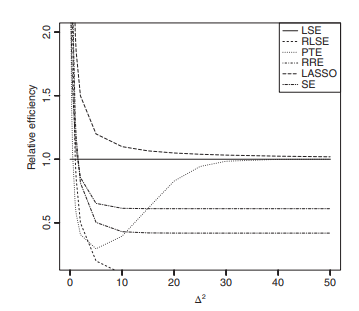
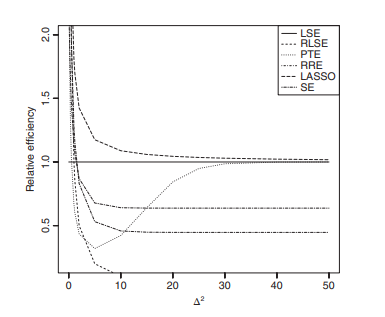
In this chapter, we are interested in studying three penalty estimators, namely,
(i) the subset rule called “hard threshold estimator” (HTE),
(ii) LASSO or the “soft threshold estimator” (STE),
(iii) the “ridge regression estimator” (RRE),
(iv) the classical PTE and shrinkage estimators such as “Stein estimator” (SE) and “positive-rule Stein-type estimator” (PRSE).

统计代写|似然估计作业代写Probability and Estimation代考|Penalty Estimators

In this section, we discuss the penalty estimators. Define the HTE as
$$
\begin{aligned}
\hat{\boldsymbol{\theta}}{n}^{\mathrm{HT}}(\kappa) &=\left(\tilde{\theta}{j n} I\left(\left|\tilde{\theta}{j n}\right|>\kappa \sigma n{j}^{-\frac{1}{2}}\right) \mid j=1, \ldots, p\right)^{\top} \
&=\left(\sigma n_{j}^{-\frac{1}{2}} \mathcal{Z}{j} I\left(\left|\mathcal{Z}{j}\right|>\kappa\right) \mid j=1, \ldots, p\right)^{\top}
\end{aligned}
$$
where $\kappa$ is a positive threshold parameter.
This estimator is discrete in nature and may be extremely variable and unstable due to the fact that small changes in the data can result in very different models and can reduce the prediction accuracy. As such we obtain the continuous version of $\hat{\theta}{n}^{\mathrm{HT}}(\kappa)$, and the LASSO is defined by $$ \hat{\boldsymbol{\theta}}{n}^{\mathrm{L}}(\lambda)=\operatorname{argmin}{\theta}(\boldsymbol{Y}-\boldsymbol{B} \boldsymbol{\theta})^{\top}(\boldsymbol{Y}-\boldsymbol{B} \theta)+2 \lambda \sigma \sum{j=1}^{p} \sqrt{n_{j}} \kappa\left|\theta_{j}\right|,
$$
where $|\theta|=\left(\left|\theta_{1}\right|, \ldots,\left|\theta_{p}\right|\right)^{\mathrm{T}}$, yielding the equation
$$
\boldsymbol{B}^{\top} \boldsymbol{B} \boldsymbol{\theta}-\boldsymbol{B}^{\top} \boldsymbol{Y}+\lambda \sigma \boldsymbol{N}^{\frac{1}{2}} \operatorname{sgn}(\boldsymbol{\theta})=\mathbf{0}
$$
or
$$
\hat{\boldsymbol{\theta}}{n}^{\mathrm{L}}(\lambda)-\tilde{\boldsymbol{\theta}}{n}+\frac{1}{2} \lambda \sigma \boldsymbol{N}^{-\frac{1}{2}} \operatorname{sgn}\left(\hat{\boldsymbol{\theta}}{n}^{\mathrm{L}}(\lambda)\right)=\mathbf{0} . $$ Now, the $j$ th component of (3.5) is given by $$ \hat{\theta}{j n}^{\mathrm{L}}(\lambda)-\ddot{\theta}{j n}+\lambda \sigma n{j}^{-\frac{1}{2}} \operatorname{sgn}\left(\hat{\theta}{j m}^{\mathrm{L}}(\lambda)\right)=0 . $$ Then, we consider three cases: (i) $\operatorname{sgn}\left(\hat{\theta}{j n}^{L}(\lambda)\right)=+1$, then, (3.6) reduces to
$$
0<\frac{\hat{\theta}{j n}^{\mathrm{L}}(\lambda)}{\sigma n{j}^{-\frac{1}{2}}}-\frac{\tilde{\theta}{j n}}{\sigma n{j}^{-\frac{1}{2}}}+\lambda=0 . $$ Hence, $$ 0<\hat{\theta}{j n}^{L}(\lambda)=\sigma n{j}^{-\frac{1}{2}}\left(Z_{j}-\lambda\right)=\sigma n_{j}^{-\frac{1}{2}}\left(\left|Z_{j}\right|-\lambda\right), $$ with, clearly, $\mathcal{Z}{j}>0$ and $\left|\mathcal{Z}{j}\right|>\lambda$.

统计代写|似然估计作业代写Probability and Estimation代考|Preliminary Test and Stein-Type Estimators

We recall that the unrestricted estimator of $\theta=\left(\theta_{1}^{\top}, \theta_{2}^{\top}\right)^{\top}$ is given by $\left(\tilde{\theta}{1 n}^{\top}, \tilde{\theta}{2 n}^{\top}\right)^{\top}$ with marginal distribution $\tilde{\theta}{1 n} \sim \mathcal{N}{p_{1}}\left(\theta_{1}, \sigma^{2} N_{1}^{-1}\right)$ and $\tilde{\theta}{2 n} \sim \mathcal{N}{p_{2}}\left(\theta_{2}, \sigma^{2} N_{2}^{-1}\right)$, respectively. The restricted estimator of $\left(\theta_{1}^{\top}, \mathbf{0}^{\top}\right)^{\top}$ is $\left(\tilde{\theta}{1 n}^{\top}, \mathbf{0}^{\top}\right)^{\top}$. Similarly, the PTE of $\theta$ is given by $$ \hat{\theta}{n}^{\mathrm{PT}}(\alpha)=\left(\begin{array}{c}
\tilde{\theta}{1 n} \ \tilde{\theta}{2 n} I\left(\mathcal{L}{n}>c{\alpha}\right)
\end{array}\right),
$$
where $I(A)$ is the indicator function of the set $A, \mathcal{L}{n}$ is the test statistic given in Section $2.2$, and $c{\alpha}$ is the $\alpha$-level critical value.
Similarly, the Stein estimator (SE) is given by
$$
\hat{\boldsymbol{\theta}}{n}^{\mathrm{S}}=\left(\begin{array}{c} \tilde{\boldsymbol{\theta}}{1 n} \
\tilde{\boldsymbol{\theta}}{2 n}\left(1-\left(p{2}-2\right) \mathcal{L}{n}^{-1}\right) \end{array}\right), \quad p{2} \geq 3
$$

and the positive-rule Stein-type estimator (PRSE) is given by
$$
\hat{\boldsymbol{\theta}}{n}^{\mathrm{S+}}=\left(\begin{array}{c} \tilde{\boldsymbol{\theta}}{1 n} \
\hat{\theta}{2 n}^{\mathrm{S}} I\left(\mathcal{L}{n}>p_{2}-2\right)
\end{array}\right)
$$

似然估计代考

统计代写|似然估计作业代写Probability and Estimation代考|Test of Significance

对于测试H这:θ2=0对比H一种:θ2≠0，我们考虑统计量大号n由大号n=1σ2θ~2n⊤ñ2θ~2n, 如果 σ2 已知  =1p2sn2θ~2n⊤ñ2θ~2n, 如果 σ2 是未知的。 在零假设下H0, 的零分布大号n是中央χ2分布与p2东风。什么时候σ2众所周知，中央F-分布与(p2,米)DE的情况下σ2分别是未知的。在备择假设下，H一种, 检验统计量大号n遵循上述密度的非中心版本。在这两种情况下，非中心性参数都是Δ2=θ2⊤ñ2θ2/σ2. 在本文中，我们始终假设σ2是已知的，那么大号n遵循卡方分布p2DF.
此外，我们注意到
θ~jn∼ñ(θj,σ2nj−1),j=1,…,p
以便从j=njθ~jn/σ∼ñ(Δj,1)， 在哪里Δj=njθj/σ. 因此，可以使用从j检验零假设H这(j):θj=0对比H一种(j):θj≠0,j=p1+1,…,p.

在本章中，我们有兴趣研究三个惩罚估计器，即
（i）称为“硬阈值估计器”（HTE）的子集规则，
（ii）LASSO 或“软阈值估计器”（STE），
（iii） “岭回归估计器”（RRE），
（iv）经典的 PTE 和收缩估计器，例如“Stein 估计器”（SE）和“正规则 Stein 型估计器”（PRSE）。

统计代写|似然估计作业代写Probability and Estimation代考|Penalty Estimators

在本节中，我们将讨论惩罚估计量。将 HTE 定义为
θ^nH吨(ķ)=(θ~jn一世(|θ~jn|>ķσnj−12)∣j=1,…,p)⊤ =(σnj−12从j一世(|从j|>ķ)∣j=1,…,p)⊤
在哪里ķ是一个正阈值参数。
该估计量本质上是离散的，并且可能非常多变和不稳定，因为数据中的微小变化可能导致非常不同的模型并可能降低预测精度。因此，我们获得了连续版本θ^nH吨(ķ), LASSO 定义为θ^n大号(λ)=精氨酸⁡θ(是−乙θ)⊤(是−乙θ)+2λσ∑j=1pnjķ|θj|,
在哪里|θ|=(|θ1|,…,|θp|)吨, 产生方程
乙⊤乙θ−乙⊤是+λσñ12sgn⁡(θ)=0
或者
θ^n大号(λ)−θ~n+12λσñ−12sgn⁡(θ^n大号(λ))=0.现在j(3.5) 的第 th 个分量由下式给出θ^jn大号(λ)−θ¨jn+λσnj−12sgn⁡(θ^j米大号(λ))=0.然后，我们考虑三种情况：（i）sgn⁡(θ^jn大号(λ))=+1，那么，(3.6) 式简化为
0<θ^jn大号(λ)σnj−12−θ~jnσnj−12+λ=0.因此，0<θ^jn大号(λ)=σnj−12(从j−λ)=σnj−12(|从j|−λ),显然，从j>0和|从j|>λ.

统计代写|似然估计作业代写Probability and Estimation代考|Preliminary Test and Stein-Type Estimators

我们记得，无限制估计θ=(θ1⊤,θ2⊤)⊤是（谁）给的(θ~1n⊤,θ~2n⊤)⊤边际分布θ~1n∼ñp1(θ1,σ2ñ1−1)和θ~2n∼ñp2(θ2,σ2ñ2−1)， 分别。的受限估计量(θ1⊤,0⊤)⊤是(θ~1n⊤,0⊤)⊤. 同样，PTEθ是（谁）给的θ^n磷吨(一种)=(θ~1n θ~2n一世(大号n>C一种)),
在哪里一世(一种)是集合的指示函数一种,大号n是第节中给出的检验统计量2.2， 和C一种是个一种级临界值。
类似地，Stein 估计量 (SE) 由下式给出
θ^n小号=(θ~1n θ~2n(1−(p2−2)大号n−1)),p2≥3

并且正规则 Stein 型估计器 (PRSE) 由下式给出
θ^n小号+=(θ~1n θ^2n小号一世(大号n>p2−2))

统计代写请认准statistics-lab™. statistics-lab™为您的留学生涯保驾护航。

金融工程代写

金融工程是使用数学技术来解决金融问题。金融工程使用计算机科学、统计学、经济学和应用数学领域的工具和知识来解决当前的金融问题，以及设计新的和创新的金融产品。

非参数统计代写

非参数统计指的是一种统计方法，其中不假设数据来自于由少数参数决定的规定模型；这种模型的例子包括正态分布模型和线性回归模型。

广义线性模型代考

广义线性模型（GLM）归属统计学领域，是一种应用灵活的线性回归模型。该模型允许因变量的偏差分布有除了正态分布之外的其它分布。

术语 广义线性模型（GLM）通常是指给定连续和/或分类预测因素的连续响应变量的常规线性回归模型。它包括多元线性回归，以及方差分析和方差分析（仅含固定效应）。

有限元方法代写

有限元方法（FEM）是一种流行的方法，用于数值解决工程和数学建模中出现的微分方程。典型的问题领域包括结构分析、传热、流体流动、质量运输和电磁势等传统领域。

有限元是一种通用的数值方法，用于解决两个或三个空间变量的偏微分方程（即一些边界值问题）。为了解决一个问题，有限元将一个大系统细分为更小、更简单的部分，称为有限元。这是通过在空间维度上的特定空间离散化来实现的，它是通过构建对象的网格来实现的：用于求解的数值域，它有有限数量的点。边界值问题的有限元方法表述最终导致一个代数方程组。该方法在域上对未知函数进行逼近。[1] 然后将模拟这些有限元的简单方程组合成一个更大的方程系统，以模拟整个问题。然后，有限元通过变化微积分使相关的误差函数最小化来逼近一个解决方案。

tatistics-lab作为专业的留学生服务机构，多年来已为美国、英国、加拿大、澳洲等留学热门地的学生提供专业的学术服务，包括但不限于Essay代写，Assignment代写，Dissertation代写，Report代写，小组作业代写，Proposal代写，Paper代写，Presentation代写，计算机作业代写，论文修改和润色，网课代做，exam代考等等。写作范围涵盖高中，本科，研究生等海外留学全阶段，辐射金融，经济学，会计学，审计学，管理学等全球99%专业科目。写作团队既有专业英语母语作者，也有海外名校硕博留学生，每位写作老师都拥有过硬的语言能力，专业的学科背景和学术写作经验。我们承诺100%原创，100%专业，100%准时，100%满意。

随机分析代写

随机微积分是数学的一个分支，对随机过程进行操作。它允许为随机过程的积分定义一个关于随机过程的一致的积分理论。这个领域是由日本数学家伊藤清在第二次世界大战期间创建并开始的。

时间序列分析代写

随机过程，是依赖于参数的一组随机变量的全体，参数通常是时间。 随机变量是随机现象的数量表现，其时间序列是一组按照时间发生先后顺序进行排列的数据点序列。通常一组时间序列的时间间隔为一恒定值（如1秒，5分钟，12小时，7天，1年），因此时间序列可以作为离散时间数据进行分析处理。研究时间序列数据的意义在于现实中，往往需要研究某个事物其随时间发展变化的规律。这就需要通过研究该事物过去发展的历史记录，以得到其自身发展的规律。

回归分析代写

多元回归分析渐进（Multiple Regression Analysis Asymptotics）属于计量经济学领域，主要是一种数学上的统计分析方法，可以分析复杂情况下各影响因素的数学关系，在自然科学、社会和经济学等多个领域内应用广泛。

MATLAB代写

MATLAB 是一种用于技术计算的高性能语言。它将计算、可视化和编程集成在一个易于使用的环境中，其中问题和解决方案以熟悉的数学符号表示。典型用途包括：数学和计算算法开发建模、仿真和原型制作数据分析、探索和可视化科学和工程图形应用程序开发，包括图形用户界面构建MATLAB 是一个交互式系统，其基本数据元素是一个不需要维度的数组。这使您可以解决许多技术计算问题，尤其是那些具有矩阵和向量公式的问题，而只需用 C 或 Fortran 等标量非交互式语言编写程序所需的时间的一小部分。MATLAB 名称代表矩阵实验室。MATLAB 最初的编写目的是提供对由 LINPACK 和 EISPACK 项目开发的矩阵软件的轻松访问，这两个项目共同代表了矩阵计算软件的最新技术。MATLAB 经过多年的发展，得到了许多用户的投入。在大学环境中，它是数学、工程和科学入门和高级课程的标准教学工具。在工业领域，MATLAB 是高效研究、开发和分析的首选工具。MATLAB 具有一系列称为工具箱的特定于应用程序的解决方案。对于大多数 MATLAB 用户来说非常重要，工具箱允许您学习和应用专业技术。工具箱是 MATLAB 函数（M 文件）的综合集合，可扩展 MATLAB 环境以解决特定类别的问题。可用工具箱的领域包括信号处理、控制系统、神经网络、模糊逻辑、小波、仿真等。

R语言代写	问卷设计与分析代写
PYTHON代写	回归分析与线性模型代写
MATLAB代写	方差分析与试验设计代写
STATA代写	机器学习/统计学习代写
SPSS代写	计量经济学代写
EVIEWS代写	时间序列分析代写
EXCEL代写	深度学习代写
SQL代写	各种数据建模与可视化代写

如果你也在 怎样代写似然估计Probability and Estimation这个学科遇到相关的难题，请随时右上角联系我们的24/7代写客服。

似然估计是一种统计方法，它用来求一个样本集的相关概率密度函数的参数。

statistics-lab™ 为您的留学生涯保驾护航 在代写似然估计Probability and Estimation方面已经树立了自己的口碑, 保证靠谱, 高质且原创的统计Statistics代写服务。我们的专家在代写似然估计Probability and Estimation代写方面经验极为丰富，各种代写似然估计Probability and Estimation相关的作业也就用不着说。

我们提供的似然估计Probability and Estimation及其相关学科的代写，服务范围广, 其中包括但不限于:

• Statistical Inference 统计推断
• Statistical Computing 统计计算
• Advanced Probability Theory 高等楖率论
• Advanced Mathematical Statistics 高等数理统计学
• (Generalized) Linear Models 广义线性模型
• Statistical Machine Learning 统计机器学习
• Longitudinal Data Analysis 纵向数据分析
• Foundations of Data Science 数据科学基础

统计代写|似然估计作业代写Probability and Estimation代考|Introduction

An important model belonging to the class of general linear hypothesis is the analysis of variance (ANOVA) model. In this model, we consider the assessment of $p$ treatment effects by considering sample experiments of sizes $n_{1}$, $n_{2}, \ldots, n_{p}$, respectively, with the responses $\left{\left(y_{i 1}, \ldots, y_{i n_{i}}\right)^{\mathrm{T}} ; i=1,2, \ldots, p\right}$ which satisfy the model, $y_{i j}=\theta_{i}+e_{i j}\left(j=1, \ldots, n_{i}, i=1, \ldots, p\right)$. The main objective of the chapter is the selection of the treatments which would yield best results. Accordingly, we consider the penalty estimators, namely, ridge, subset selection rule, and least absolute shrinkage and selection operator (LASSO) together with the classical shrinkage estimators, namely, the preliminary test estimator (PTE), the Stein-type estimators (SE), and positive-rule Stein-type estimator (PRSE) of $\theta=\left(\theta_{1}, \ldots, \theta_{p}\right)^{\top}$. For LASSO and related methods, see Breiman (1996), Fan and Li (2001), Zou and Hastie (2005), and Zou (2006), among others; and for PTE and SE, see Judge and Bock (1978) and Saleh (2006), among others.

The chapter points to the useful “selection” aspect of LASSO and ridge estimators as well as limitations found in other papers. Our conclusions are based on the ideal $\mathrm{L}{2}$ risk of LASSO of an oracle which would supply optimal coefficients in a diagonal projection scheme given by Donoho and Johnstone (1994, p. 437). The comparison of the estimators considered here are based on mathematical analysis as well as by tables of $\mathrm{L}{2}$-risk efficiencies and graphs and not by simulation.

In his pioneering paper, Tibshirani (1996) examined the relative performance of the subset selection, ridge regression, and LASSO in three different scenarios, under orthogonal design matrix in a linear regression model:
(a) Small number of large coefficients: subset selection does the best here, the LASSO not quite as well, ridge regression does quite poorly.
(b) Small to moderate numbers of moderate-size coefficients: LASSO does the best, followed by ridge regression and then subset selection.

统计代写|似然估计作业代写Probability and Estimation代考|Model, Estimation, and Tests

Consider the ANOVA model
$$
\boldsymbol{Y}=\boldsymbol{B} \boldsymbol{\theta}+\boldsymbol{\epsilon}=\boldsymbol{B}{1} \boldsymbol{\theta}{1}+\boldsymbol{B}{2} \boldsymbol{\theta}{2}+\boldsymbol{\epsilon},
$$
where $Y=\left(y_{11}, \ldots, y_{1 n_{1}}, \ldots, y_{p_{1}}, \ldots, y_{p w_{p}}\right)^{\top}, \theta=\left(\theta_{1}, \ldots, \theta_{p_{1}}, \theta_{p_{1}+1}, \ldots, \theta_{p}\right)^{\top}$ is the unknown vector that can be partitioned as $\boldsymbol{\theta}=\left(\boldsymbol{\theta}{1}^{\top}, \boldsymbol{\theta}{2}^{\top}\right)^{\top}$, where $\boldsymbol{\theta}{1}=$ $\left(\theta{1}, \ldots, \theta_{p_{1}}\right)^{\top}$, and $\theta_{2}=\left(\theta_{p_{1}+1}, \ldots, \theta_{p}\right)^{\top}$.

The error vector $\boldsymbol{\epsilon}$ is $\left(\epsilon_{11}, \ldots, \epsilon_{1 n_{1}}, \ldots, \epsilon_{p_{1}}, \ldots, \epsilon_{p v_{p}}\right)^{\top}$ with $\boldsymbol{E} \sim \mathcal{N}{n}\left(\mathbf{0}, \sigma^{2} I{n}\right)$. The notation $B$ stands for a block-diagonal vector of $\left(\mathbf{1}{n{1}}, \ldots, \mathbf{1}{n{p}}\right)$ which can subdivide into two matrices $\boldsymbol{B}{1}$ and $\boldsymbol{B}{2}$ as $\left(\boldsymbol{B}{1}, \boldsymbol{B}{2}\right)$, where $\mathbf{1}{n{j}}=(1, \ldots, 1)^{\top}$ is an $n_{i}$-tuples of $1 \mathrm{~s}, \boldsymbol{I}{n}$ is the $n$-dimensional identity matrix where $n=n{1}+\cdots+n_{p}$, and $\sigma^{2}$ is the known variance of the errors.

Our objective is to estimate and select the treatments $\theta=\left(\theta_{1}, \ldots, \theta_{p}\right)^{\top}$ when we suspect that the subset $\theta_{2}=\left(\theta_{p_{1}+1}, \ldots, \theta_{p}\right)^{\top}$ may be $\mathbf{0}$, i.e. ineffective. Thus, we consider the model (3.1) and discuss the LSE of $\theta$ in Section 3.2.1.

统计代写|似然估计作业代写Probability and Estimation代考|Estimation of Treatment Effects

First, we consider the unrestricted LSE of $\theta=\left(\theta_{1}^{\top}, \theta_{2}^{\top}\right)^{\top}$ given by
$\tilde{\theta}{n}=\operatorname{argmin}{\theta}\left{\left(\boldsymbol{Y}-\boldsymbol{B}{1} \boldsymbol{\theta}{1}-\boldsymbol{B}{2} \boldsymbol{\theta}{2}\right)^{\top}\left(\boldsymbol{Y}-\boldsymbol{B}{1} \boldsymbol{\theta}{1}-\boldsymbol{B}{2} \boldsymbol{\theta}{2}\right)\right}$
$=\left(\begin{array}{cc}\boldsymbol{B}{1}^{\top} \boldsymbol{B}{1} & \boldsymbol{B}{1}^{\top} \boldsymbol{B}{2} \ \boldsymbol{B}{2}^{\top} \boldsymbol{B}{1} & \boldsymbol{B}{2}^{\top} \boldsymbol{B}{2}\end{array}\right)^{-1}\left(\begin{array}{c}\boldsymbol{B}{1}^{\top} \boldsymbol{Y} \ \boldsymbol{B}{2}^{\top} \boldsymbol{Y}\end{array}\right)=\left(\begin{array}{cc}\boldsymbol{N}{1} & \mathbf{0} \ \mathbf{0} & \boldsymbol{N}{2}\end{array}\right)^{-1}\left(\begin{array}{c}\boldsymbol{B}{1}^{\top} \boldsymbol{Y} \ \boldsymbol{B}{2}^{\top} \boldsymbol{Y}\end{array}\right)$
$=\left(\begin{array}{c}\boldsymbol{N}{1}^{-1} \boldsymbol{B}{1}^{\top} \boldsymbol{Y} \ \boldsymbol{N}{2}^{-1} \boldsymbol{B}{2}^{\top} \boldsymbol{Y}\end{array}\right)=\left(\begin{array}{l}\tilde{\boldsymbol{\theta}}{1 n} \ \tilde{\boldsymbol{\theta}}{2 n}\end{array}\right)$,
where $\boldsymbol{N}=\boldsymbol{B}^{\top} \boldsymbol{B}=\operatorname{Diag}\left(n_{1}, \ldots, n_{p}\right), \quad \boldsymbol{N}{1}=\operatorname{Diag}\left(n{1}, \ldots, n_{p_{1}}\right), \quad$ and $\quad \boldsymbol{N}{2}=$ $\operatorname{Diag}\left(n{p_{1}+1}, \ldots, n_{p}\right)$.

In case $\sigma^{2}$ is unknown, the best linear unbiased estimator (BLUE) of $\sigma^{2}$ is given by
$$
s_{n}^{2}=(n-p)^{-1}\left(\boldsymbol{Y}-\boldsymbol{B}{1} \tilde{\theta}{1 n}-\boldsymbol{B}{2} \tilde{\theta}{2 n}\right)^{\top}\left(\boldsymbol{Y}-\boldsymbol{B}{1} \tilde{\theta}{1 n}-\boldsymbol{B}{2} \tilde{\theta}{2 n}\right) .
$$
Clearly, $\tilde{\theta}{n} \sim \mathcal{N}{p}\left(\theta, \sigma^{2} N^{-1}\right)$ is independent of $m s_{n}^{2} / \sigma^{2}(m=n-p)$, which follows a central $\chi^{2}$ distribution with $m$ degrees of freedom (DF).

When $\theta_{2}=\mathbf{0}$, the restricted least squares estimator (RLSE) of $\theta_{\mathrm{R}}=\left(\theta_{1}^{\top}, \mathbf{0}^{\top}\right)^{\top}$ is given by $\hat{\boldsymbol{\theta}}{\mathrm{R}}=\left(\tilde{\boldsymbol{\theta}}{1 n}^{\top}, \boldsymbol{0}^{\top}\right)^{\top}$, where $\tilde{\boldsymbol{\theta}}{1 n}=\boldsymbol{N}{1}^{-1} \boldsymbol{B}_{1}^{\top} \boldsymbol{Y}$.

似然估计代考

统计代写|似然估计作业代写Probability and Estimation代考|Introduction

属于一般线性假设类的一个重要模型是方差分析（ANOVA）模型。在这个模型中，我们考虑评估p考虑大小样本实验的处理效果n1, n2,…,np，分别与响应\left{\left(y_{i 1}, \ldots, y_{i n_{i}}\right)^{\mathrm{T}} ; i=1,2, \ldots, p\right}\left{\left(y_{i 1}, \ldots, y_{i n_{i}}\right)^{\mathrm{T}} ; i=1,2, \ldots, p\right}满足模型，是一世j=θ一世+和一世j(j=1,…,n一世,一世=1,…,p). 本章的主要目标是选择能产生最佳结果的处理方法。因此，我们考虑惩罚估计量，即岭、子集选择规则和最小绝对收缩和选择算子（LASSO）以及经典收缩估计量，即初步测试估计量（PTE）、斯坦型估计量（SE ) 和正规则 Stein 型估计器 (PRSE)θ=(θ1,…,θp)⊤. LASSO 及相关方法见 Breiman (1996), Fan and Li (2001), Zou and Hastie (2005), and Zou (2006) 等；对于 PTE 和 SE，请参见 Judge and Bock (1978) 和 Saleh (2006) 等。

本章指出了 LASSO 和岭估计器的有用“选择”方面以及其他论文中发现的局限性。我们的结论是基于理想的大号2预言机的 LASSO 风险，它将在 Donoho 和 Johnstone 给出的对角投影方案中提供最佳系数（1994 年，第 437 页）。这里考虑的估计量的比较是基于数学分析以及表格大号2-风险效率和图表，而不是模拟。

在他的开创性论文中，Tibshirani (1996) 在线性回归模型中的正交设计矩阵下检查了子集选择、岭回归和 LASSO 在三种不同场景中的相对性能：
(a) 少量大系数：子集选择确实这里最好，LASSO 不太好，岭回归的效果很差。
(b) 小到中等数量的中等大小的系数：LASSO 做得最好，其次是岭回归，然后是子集选择。

统计代写|似然估计作业代写Probability and Estimation代考|Model, Estimation, and Tests

考虑方差分析模型
是=乙θ+ε=乙1θ1+乙2θ2+ε,
在哪里是=(是11,…,是1n1,…,是p1,…,是p在p)⊤,θ=(θ1,…,θp1,θp1+1,…,θp)⊤是可以划分为的未知向量θ=(θ1⊤,θ2⊤)⊤， 在哪里θ1= (θ1,…,θp1)⊤， 和θ2=(θp1+1,…,θp)⊤.

误差向量ε是(ε11,…,ε1n1,…,εp1,…,εp在p)⊤和和∼ñn(0,σ2一世n). 符号乙代表块对角向量(1n1,…,1np)可以细分为两个矩阵乙1和乙2作为(乙1,乙2)， 在哪里1nj=(1,…,1)⊤是一个n一世- 元组1 s,一世n是个n维单位矩阵，其中n=n1+⋯+np， 和σ2是误差的已知方差。

我们的目标是估计和选择治疗θ=(θ1,…,θp)⊤当我们怀疑子集θ2=(θp1+1,…,θp)⊤或许0，即无效。因此，我们考虑模型（3.1）并讨论 LSEθ在第 3.2.1 节中。

统计代写|似然估计作业代写Probability and Estimation代考|Estimation of Treatment Effects

首先，我们考虑不受限制的 LSEθ=(θ1⊤,θ2⊤)⊤由
\tilde{\theta}{n}=\operatorname{argmin}{\theta}\left{\left(\boldsymbol{Y}-\boldsymbol{B}{1} \boldsymbol{\theta}{1}-\ boldsymbol{B}{2} \boldsymbol{\theta}{2}\right)^{\top}\left(\boldsymbol{Y}-\boldsymbol{B}{1} \boldsymbol{\theta}{1} -\boldsymbol{B}{2} \boldsymbol{\theta}{2}\right)\right}\tilde{\theta}{n}=\operatorname{argmin}{\theta}\left{\left(\boldsymbol{Y}-\boldsymbol{B}{1} \boldsymbol{\theta}{1}-\ boldsymbol{B}{2} \boldsymbol{\theta}{2}\right)^{\top}\left(\boldsymbol{Y}-\boldsymbol{B}{1} \boldsymbol{\theta}{1} -\boldsymbol{B}{2} \boldsymbol{\theta}{2}\right)\right}
=(乙1⊤乙1乙1⊤乙2 乙2⊤乙1乙2⊤乙2)−1(乙1⊤是 乙2⊤是)=(ñ10 0ñ2)−1(乙1⊤是 乙2⊤是)
=(ñ1−1乙1⊤是 ñ2−1乙2⊤是)=(θ~1n θ~2n),
其中ñ=乙⊤乙=诊断⁡(n1,…,np),ñ1=诊断⁡(n1,…,np1),和ñ2= 诊断⁡(np1+1,…,np).

如果σ2是未知的，最佳线性无偏估计量 (BLUE)σ2是（谁）给的
sn2=(n−p)−1(是−乙1θ~1n−乙2θ~2n)⊤(是−乙1θ~1n−乙2θ~2n).
清楚地，θ~n∼ñp(θ,σ2ñ−1)独立于米sn2/σ2(米=n−p)，它遵循一个中心χ2分布与米自由度 (DF)。

什么时候θ2=0, 的受限最小二乘估计量 (RLSE)θR=(θ1⊤,0⊤)⊤是（谁）给的θ^R=(θ~1n⊤,0⊤)⊤， 在哪里θ~1n=ñ1−1乙1⊤是.

统计代写请认准statistics-lab™. statistics-lab™为您的留学生涯保驾护航。

金融工程代写

金融工程是使用数学技术来解决金融问题。金融工程使用计算机科学、统计学、经济学和应用数学领域的工具和知识来解决当前的金融问题，以及设计新的和创新的金融产品。

非参数统计代写

非参数统计指的是一种统计方法，其中不假设数据来自于由少数参数决定的规定模型；这种模型的例子包括正态分布模型和线性回归模型。

广义线性模型代考

广义线性模型（GLM）归属统计学领域，是一种应用灵活的线性回归模型。该模型允许因变量的偏差分布有除了正态分布之外的其它分布。

术语 广义线性模型（GLM）通常是指给定连续和/或分类预测因素的连续响应变量的常规线性回归模型。它包括多元线性回归，以及方差分析和方差分析（仅含固定效应）。

有限元方法代写

有限元方法（FEM）是一种流行的方法，用于数值解决工程和数学建模中出现的微分方程。典型的问题领域包括结构分析、传热、流体流动、质量运输和电磁势等传统领域。

有限元是一种通用的数值方法，用于解决两个或三个空间变量的偏微分方程（即一些边界值问题）。为了解决一个问题，有限元将一个大系统细分为更小、更简单的部分，称为有限元。这是通过在空间维度上的特定空间离散化来实现的，它是通过构建对象的网格来实现的：用于求解的数值域，它有有限数量的点。边界值问题的有限元方法表述最终导致一个代数方程组。该方法在域上对未知函数进行逼近。[1] 然后将模拟这些有限元的简单方程组合成一个更大的方程系统，以模拟整个问题。然后，有限元通过变化微积分使相关的误差函数最小化来逼近一个解决方案。

tatistics-lab作为专业的留学生服务机构，多年来已为美国、英国、加拿大、澳洲等留学热门地的学生提供专业的学术服务，包括但不限于Essay代写，Assignment代写，Dissertation代写，Report代写，小组作业代写，Proposal代写，Paper代写，Presentation代写，计算机作业代写，论文修改和润色，网课代做，exam代考等等。写作范围涵盖高中，本科，研究生等海外留学全阶段，辐射金融，经济学，会计学，审计学，管理学等全球99%专业科目。写作团队既有专业英语母语作者，也有海外名校硕博留学生，每位写作老师都拥有过硬的语言能力，专业的学科背景和学术写作经验。我们承诺100%原创，100%专业，100%准时，100%满意。

随机分析代写

随机微积分是数学的一个分支，对随机过程进行操作。它允许为随机过程的积分定义一个关于随机过程的一致的积分理论。这个领域是由日本数学家伊藤清在第二次世界大战期间创建并开始的。

时间序列分析代写

随机过程，是依赖于参数的一组随机变量的全体，参数通常是时间。 随机变量是随机现象的数量表现，其时间序列是一组按照时间发生先后顺序进行排列的数据点序列。通常一组时间序列的时间间隔为一恒定值（如1秒，5分钟，12小时，7天，1年），因此时间序列可以作为离散时间数据进行分析处理。研究时间序列数据的意义在于现实中，往往需要研究某个事物其随时间发展变化的规律。这就需要通过研究该事物过去发展的历史记录，以得到其自身发展的规律。

回归分析代写

多元回归分析渐进（Multiple Regression Analysis Asymptotics）属于计量经济学领域，主要是一种数学上的统计分析方法，可以分析复杂情况下各影响因素的数学关系，在自然科学、社会和经济学等多个领域内应用广泛。

MATLAB代写

MATLAB 是一种用于技术计算的高性能语言。它将计算、可视化和编程集成在一个易于使用的环境中，其中问题和解决方案以熟悉的数学符号表示。典型用途包括：数学和计算算法开发建模、仿真和原型制作数据分析、探索和可视化科学和工程图形应用程序开发，包括图形用户界面构建MATLAB 是一个交互式系统，其基本数据元素是一个不需要维度的数组。这使您可以解决许多技术计算问题，尤其是那些具有矩阵和向量公式的问题，而只需用 C 或 Fortran 等标量非交互式语言编写程序所需的时间的一小部分。MATLAB 名称代表矩阵实验室。MATLAB 最初的编写目的是提供对由 LINPACK 和 EISPACK 项目开发的矩阵软件的轻松访问，这两个项目共同代表了矩阵计算软件的最新技术。MATLAB 经过多年的发展，得到了许多用户的投入。在大学环境中，它是数学、工程和科学入门和高级课程的标准教学工具。在工业领域，MATLAB 是高效研究、开发和分析的首选工具。MATLAB 具有一系列称为工具箱的特定于应用程序的解决方案。对于大多数 MATLAB 用户来说非常重要，工具箱允许您学习和应用专业技术。工具箱是 MATLAB 函数（M 文件）的综合集合，可扩展 MATLAB 环境以解决特定类别的问题。可用工具箱的领域包括信号处理、控制系统、神经网络、模糊逻辑、小波、仿真等。

R语言代写	问卷设计与分析代写
PYTHON代写	回归分析与线性模型代写
MATLAB代写	方差分析与试验设计代写
STATA代写	机器学习/统计学习代写
SPSS代写	计量经济学代写
EVIEWS代写	时间序列分析代写
EXCEL代写	深度学习代写
SQL代写	各种数据建模与可视化代写

如果你也在 怎样代写似然估计Probability and Estimation这个学科遇到相关的难题，请随时右上角联系我们的24/7代写客服。

似然估计是一种统计方法，它用来求一个样本集的相关概率密度函数的参数。

statistics-lab™ 为您的留学生涯保驾护航 在代写似然估计Probability and Estimation方面已经树立了自己的口碑, 保证靠谱, 高质且原创的统计Statistics代写服务。我们的专家在代写似然估计Probability and Estimation代写方面经验极为丰富，各种代写似然估计Probability and Estimation相关的作业也就用不着说。

我们提供的似然估计Probability and Estimation及其相关学科的代写，服务范围广, 其中包括但不限于:

• Statistical Inference 统计推断
• Statistical Computing 统计计算
• Advanced Probability Theory 高等楖率论
• Advanced Mathematical Statistics 高等数理统计学
• (Generalized) Linear Models 广义线性模型
• Statistical Machine Learning 统计机器学习
• Longitudinal Data Analysis 纵向数据分析
• Foundations of Data Science 数据科学基础

统计代写|似然估计作业代写Probability and Estimation代考|Bias and MSE Expressions

From (2.65), it is easy to see that the bias expression of $\hat{\theta}{n}^{\mathrm{RR}}(k)$ and $\hat{\beta}{n}^{\mathrm{RR}}(k)$, respectively, are given by
$$
\begin{aligned}
&b\left(\hat{\theta}{n}^{\mathrm{RR}}(k)\right)=-\frac{k}{Q+k} \beta \bar{x} \ &b\left(\hat{\beta}{n}^{\mathrm{RR}}(k)\right)=-\frac{k}{Q+k} \beta .
\end{aligned}
$$
Similarly, MSE expressions of the estimators are given by
$$
\begin{aligned}
\operatorname{MSE}\left(\hat{\theta}{n}^{\mathrm{RR}}(k)\right) &=\frac{\sigma^{2}}{n}\left(1+\frac{n \bar{x}^{2} Q}{(Q+k)^{2}}\right)+\frac{k^{2} \beta^{2} \bar{x}^{2}}{(Q+k)^{2}} \ &=\frac{\sigma^{2}}{n}\left{\left(1+\frac{n \bar{x}^{2} Q}{(Q+k)^{2}}\right)+\frac{n \bar{x}^{2} k^{2} \beta^{2}}{(Q+k)^{2} \sigma^{2}}\right} \ &=\frac{\sigma^{2}}{n}\left{1+\frac{n \bar{x}^{2}}{Q(Q+k)^{2}}\left(Q^{2}+k^{2} \Delta^{2}\right)\right} \end{aligned} $$ where $\Delta^{2}=\frac{Q \rho^{2}}{\sigma^{2}}$ and $$ \begin{aligned} \operatorname{MSE}\left(\hat{\beta}{n}^{\mathrm{RR}}(k)\right) &=\frac{\sigma^{2} Q}{(Q+k)^{2}}+\frac{k^{2} \beta^{2}}{(Q+k)^{2}} \
&=\frac{\sigma^{2}}{Q(Q+k)^{2}}\left(Q^{2}+k^{2} \Delta^{2}\right) .
\end{aligned}
$$
Hence, the REff of these estimators are given by
$$
\begin{aligned}
\operatorname{REff}\left(\hat{\theta}{n}^{\mathrm{RR}}(k): \tilde{\theta}{n}\right) &=\left(1+\frac{n \bar{x}^{2}}{Q}\right)\left{1+\frac{n \bar{x}^{2}}{Q(Q+k)^{2}}\left(Q^{2}+k^{2} \Delta^{2}\right)\right}^{-1} \
\operatorname{REff}\left(\hat{\beta}{n}^{\mathrm{RR}}(k): \tilde{\beta}{n}\right) &=(Q+k)^{2}\left(Q^{2}+k \Delta^{2}\right)^{-1} \
&=\left(1+\frac{k}{Q}\right)\left{1+\frac{k \Delta^{2}}{Q^{2}}\right}^{-1}
\end{aligned}
$$

Note that the optimum value of $k$ is $Q \Delta^{-2}$. Hence,
$$
\begin{aligned}
\operatorname{MSE}\left(\hat{\theta}{n}^{\mathrm{RR}}\left(Q \Delta^{-2}\right)\right) &=\frac{\sigma^{2}}{n}\left(1+\frac{n \bar{x}^{2} \Delta^{2}}{Q\left(1+\Delta^{2}\right)}\right) \ \operatorname{REff}\left(\hat{\theta}{n}^{\mathrm{RR}}\left(Q \Delta^{-2}\right): \tilde{\theta}{n}\right) &=\left(1+\frac{n \bar{x}^{2}}{Q}\right)\left{1+\frac{n \bar{x}^{2} \Delta^{2}}{Q\left(1+\Delta^{2}\right)}\right}^{-1} \ \operatorname{MSE}\left(\hat{\beta}{n}^{\mathrm{RR}}\left(Q \Delta^{-2}\right)\right) &=\frac{\sigma^{2}}{Q}\left(\frac{1+\Delta^{2}}{\Delta^{2}}\right)\left(\frac{Q}{1+Q}\right) \
\operatorname{REff}\left(\hat{\beta}{n}^{\mathrm{RR}}\left(Q \Delta^{-2}\right): \tilde{\beta}{n}\right) &=\left(\frac{1+\Delta^{2}}{\Delta^{2}}\right)\left(\frac{Q}{1+Q}\right)
\end{aligned}
$$

统计代写|似然估计作业代写Probability and Estimation代考|LASSO Estimation of Intercept and Slope

In this section, we consider the LASSO estimation of $(\theta, \beta)$ when it is suspected that $\beta$ may be 0 . For this case, the solution is given by
$$
\left(\hat{\theta}{n}^{\mathrm{LASSO}}(\lambda), \hat{\beta}{n}^{\mathrm{LASSO}}(\lambda)\right)^{\top}=\operatorname{argmin}{(\theta), \beta}}\left{\left|Y-\theta \mathbf{1}{n}-\beta x\right|^{2}+\sqrt{Q} \lambda \sigma|\beta|\right} .
$$
Explicitly, we find
$$
\begin{aligned}
\hat{\theta}{n}^{\mathrm{LASSO}}(\lambda) &=\bar{y}-\hat{\beta}{n}^{\mathrm{LASSO}} \bar{x} \
\hat{\beta}{n}^{\mathrm{LASSO}} &=\operatorname{sgn}(\tilde{\beta})\left(|\tilde{\beta}|-\lambda \frac{\sigma}{\sqrt{Q}}\right)^{+} \ &=\frac{\sigma}{\sqrt{Q}} \operatorname{sgn}\left(Z{n}\right)\left(\left|Z_{n}\right|-\lambda\right)^{+},
\end{aligned}
$$
where $Z_{n}=\sqrt{Q} \tilde{\beta}{n} / \sigma \sim \mathcal{N}(\Delta, 1)$ and $\Delta=\sqrt{Q} \beta / \sigma$. According to Donoho and Johnstone (1994), and results of Section 2.2.5, the bias and MSE expressions for $\hat{\beta}{n}^{\mathrm{LASSO}}(\lambda)$ are given by
$$
\begin{aligned}
b\left(\hat{\beta}{n}^{\mathrm{LASSO}}(\lambda)\right)=& \frac{\sigma}{\sqrt{Q}}{\lambda[\Phi(\lambda-\Delta)-\Phi(\lambda+\Delta)]\ &+\Delta[\Phi(-\lambda-\Delta)-\Phi(\lambda-\Delta)] \ &+[\phi(\lambda-\Delta)-\phi(\lambda+\Delta)]}, \ \operatorname{MSE}\left(\hat{\beta}{n}^{\mathrm{LASSO}}(\lambda)\right)=& \frac{\sigma^{2}}{Q} \rho_{\mathrm{ST}}(\lambda, \Delta),
\end{aligned}
$$
where
$$
\begin{aligned}
\rho_{\mathrm{ST}}(\lambda, \Delta)=& 1+\lambda^{2}+\left(1-\Delta^{2}-\lambda^{2}\right){\Phi(\lambda-\Delta)-\Phi(-\lambda-\Delta)} \
&-(\lambda-\Delta) \phi(\lambda+\Delta)-(\lambda+\Delta) \phi(\lambda-\Delta)
\end{aligned}
$$

统计代写|似然估计作业代写Probability and Estimation代考|Summary and Concluding Remarks

This chapter considers the location model and the simple linear regression model when errors of the models are normally distributed. We consider LSE, RLSE, PTE, SE and two penalty estimators, namely, the RRE and the LASSO estimator for the location parameter for the location model and the intercept and slope parameter for the simple linear regression model. We found that the RRE uniformly dominates LSE, PTE, SE, and LASSO. However, RLSE dominates all estimators near the null hypothesis. LASSO dominates LSE, PTE, and SE uniformly.

似然估计代考

统计代写|似然估计作业代写Probability and Estimation代考|Bias and MSE Expressions

由式（2.65）不难看出，θ^nRR(ķ)和b^nRR(ķ)，分别由下式给出
b(θ^nRR(ķ))=−ķ问+ķbX¯ b(b^nRR(ķ))=−ķ问+ķb.
类似地，估计量的 MSE 表达式由下式给出
\begin{aligned} \operatorname{MSE}\left(\hat{\theta}{n}^{\mathrm{RR}}(k)\right) &=\frac{\sigma^{2}}{n }\left(1+\frac{n \bar{x}^{2} Q}{(Q+k)^{2}}\right)+\frac{k^{2} \beta^{2} \bar{x}^{2}}{(Q+k)^{2}} \ &=\frac{\sigma^{2}}{n}\left{\left(1+\frac{n \ bar{x}^{2} Q}{(Q+k)^{2}}\right)+\frac{n \bar{x}^{2} k^{2} \beta^{2}} {(Q+k)^{2} \sigma^{2}}\right} \ &=\frac{\sigma^{2}}{n}\left{1+\frac{n \bar{x} ^{2}}{Q(Q+k)^{2}}\left(Q^{2}+k^{2} \Delta^{2}\right)\right} \end{对齐}\begin{aligned} \operatorname{MSE}\left(\hat{\theta}{n}^{\mathrm{RR}}(k)\right) &=\frac{\sigma^{2}}{n }\left(1+\frac{n \bar{x}^{2} Q}{(Q+k)^{2}}\right)+\frac{k^{2} \beta^{2} \bar{x}^{2}}{(Q+k)^{2}} \ &=\frac{\sigma^{2}}{n}\left{\left(1+\frac{n \ bar{x}^{2} Q}{(Q+k)^{2}}\right)+\frac{n \bar{x}^{2} k^{2} \beta^{2}} {(Q+k)^{2} \sigma^{2}}\right} \ &=\frac{\sigma^{2}}{n}\left{1+\frac{n \bar{x} ^{2}}{Q(Q+k)^{2}}\left(Q^{2}+k^{2} \Delta^{2}\right)\right} \end{对齐}在哪里Δ2=问ρ2σ2和MSE⁡(b^nRR(ķ))=σ2问(问+ķ)2+ķ2b2(问+ķ)2 =σ2问(问+ķ)2(问2+ķ2Δ2).
因此，这些估计量的 REff 由下式给出
\begin{aligned} \operatorname{REff}\left(\hat{\theta}{n}^{\mathrm{RR}}(k): \tilde{\theta}{n}\right) &=\left (1+\frac{n \bar{x}^{2}}{Q}\right)\left{1+\frac{n \bar{x}^{2}}{Q(Q+k)^ {2}}\left(Q^{2}+k^{2} \Delta^{2}\right)\right}^{-1} \ \operatorname{REff}\left(\hat{\beta} {n}^{\mathrm{RR}}(k): \tilde{\beta}{n}\right) &=(Q+k)^{2}\left(Q^{2}+k \Delta ^{2}\right)^{-1} \ &=\left(1+\frac{k}{Q}\right)\left{1+\frac{k \Delta^{2}}{Q^ {2}}\right}^{-1} \end{对齐}\begin{aligned} \operatorname{REff}\left(\hat{\theta}{n}^{\mathrm{RR}}(k): \tilde{\theta}{n}\right) &=\left (1+\frac{n \bar{x}^{2}}{Q}\right)\left{1+\frac{n \bar{x}^{2}}{Q(Q+k)^ {2}}\left(Q^{2}+k^{2} \Delta^{2}\right)\right}^{-1} \ \operatorname{REff}\left(\hat{\beta} {n}^{\mathrm{RR}}(k): \tilde{\beta}{n}\right) &=(Q+k)^{2}\left(Q^{2}+k \Delta ^{2}\right)^{-1} \ &=\left(1+\frac{k}{Q}\right)\left{1+\frac{k \Delta^{2}}{Q^ {2}}\right}^{-1} \end{对齐}

请注意，最佳值ķ是问Δ−2. 因此，
\begin{aligned} \operatorname{MSE}\left(\hat{\theta}{n}^{\mathrm{RR}}\left(Q \Delta^{-2}\right)\right) &=\ frac{\sigma^{2}}{n}\left(1+\frac{n \bar{x}^{2} \Delta^{2}}{Q\left(1+\Delta^{2} \right)}\right) \ \operatorname{REff}\left(\hat{\theta}{n}^{\mathrm{RR}}\left(Q \Delta^{-2}\right): \tilde {\theta}{n}\right) &=\left(1+\frac{n \bar{x}^{2}}{Q}\right)\left{1+\frac{n \bar{x }^{2} \Delta^{2}}{Q\left(1+\Delta^{2}\right)}\right}^{-1} \ \operatorname{MSE}\left(\hat{\ beta}{n}^{\mathrm{RR}}\left(Q \Delta^{-2}\right)\right) &=\frac{\sigma^{2}}{Q}\left(\frac {1+\Delta^{2}}{\Delta^{2}}\right)\left(\frac{Q}{1+Q}\right) \ \operatorname{REff}\left(\hat{\ beta}{n}^{\mathrm{RR}}\left(Q \Delta^{-2}\right): \tilde{\beta}{n}\right) &=\left(\frac{1+ \Delta^{2}}{\Delta^{2}}\right)\left(\frac{Q}{1+Q}\right) \end{aligned}\begin{aligned} \operatorname{MSE}\left(\hat{\theta}{n}^{\mathrm{RR}}\left(Q \Delta^{-2}\right)\right) &=\ frac{\sigma^{2}}{n}\left(1+\frac{n \bar{x}^{2} \Delta^{2}}{Q\left(1+\Delta^{2} \right)}\right) \ \operatorname{REff}\left(\hat{\theta}{n}^{\mathrm{RR}}\left(Q \Delta^{-2}\right): \tilde {\theta}{n}\right) &=\left(1+\frac{n \bar{x}^{2}}{Q}\right)\left{1+\frac{n \bar{x }^{2} \Delta^{2}}{Q\left(1+\Delta^{2}\right)}\right}^{-1} \ \operatorname{MSE}\left(\hat{\ beta}{n}^{\mathrm{RR}}\left(Q \Delta^{-2}\right)\right) &=\frac{\sigma^{2}}{Q}\left(\frac {1+\Delta^{2}}{\Delta^{2}}\right)\left(\frac{Q}{1+Q}\right) \ \operatorname{REff}\left(\hat{\ beta}{n}^{\mathrm{RR}}\left(Q \Delta^{-2}\right): \tilde{\beta}{n}\right) &=\left(\frac{1+ \Delta^{2}}{\Delta^{2}}\right)\left(\frac{Q}{1+Q}\right) \end{aligned}

统计代写|似然估计作业代写Probability and Estimation代考|LASSO Estimation of Intercept and Slope

在本节中，我们考虑 LASSO 估计(θ,b)当怀疑b可能是 0 。对于这种情况，解决方案由下式给出
\left(\hat{\theta}{n}^{\mathrm{LASSO}}(\lambda), \hat{\beta}{n}^{\mathrm{LASSO}}(\lambda)\right)^ {\top}=\operatorname{argmin}{(\theta), \beta}}\left{\left|Y-\theta \mathbf{1}{n}-\beta x\right|^{2}+ \sqrt{Q} \lambda \sigma|\beta|\right} 。\left(\hat{\theta}{n}^{\mathrm{LASSO}}(\lambda), \hat{\beta}{n}^{\mathrm{LASSO}}(\lambda)\right)^ {\top}=\operatorname{argmin}{(\theta), \beta}}\left{\left|Y-\theta \mathbf{1}{n}-\beta x\right|^{2}+ \sqrt{Q} \lambda \sigma|\beta|\right} 。
明确地，我们发现
θ^n大号一种小号小号这(λ)=是¯−b^n大号一种小号小号这X¯ b^n大号一种小号小号这=sgn⁡(b~)(|b~|−λσ问)+ =σ问sgn⁡(从n)(|从n|−λ)+,
在哪里从n=问b~n/σ∼ñ(Δ,1)和Δ=问b/σ. 根据 Donoho 和 Johnstone (1994) 以及第 2.2.5 节的结果，偏差和 MSE 表达式为b^n大号一种小号小号这(λ)由
\begin{对齐} b\left(\hat{\beta}{n}^{\mathrm{LASSO}}(\lambda)\right)=& \frac{\sigma}{\sqrt{Q}}{\ λ[\Phi(\lambda-\Delta)-\Phi(\lambda+\Delta)]\ &+\Delta[\Phi(-\lambda-\Delta)-\Phi(\lambda-\Delta)] \ & +[\phi(\lambda-\Delta)-\phi(\lambda+\Delta)]}, \ \operatorname{MSE}\left(\hat{\beta}{n}^{\mathrm{LASSO}}( \lambda)\right)=& \frac{\sigma^{2}}{Q} \rho_{\mathrm{ST}}(\lambda, \Delta), \end{aligned}\begin{对齐} b\left(\hat{\beta}{n}^{\mathrm{LASSO}}(\lambda)\right)=& \frac{\sigma}{\sqrt{Q}}{\ λ[\Phi(\lambda-\Delta)-\Phi(\lambda+\Delta)]\ &+\Delta[\Phi(-\lambda-\Delta)-\Phi(\lambda-\Delta)] \ & +[\phi(\lambda-\Delta)-\phi(\lambda+\Delta)]}, \ \operatorname{MSE}\left(\hat{\beta}{n}^{\mathrm{LASSO}}( \lambda)\right)=& \frac{\sigma^{2}}{Q} \rho_{\mathrm{ST}}(\lambda, \Delta), \end{aligned}
在哪里
ρ小号吨(λ,Δ)=1+λ2+(1−Δ2−λ2)披(λ−Δ)−披(−λ−Δ) −(λ−Δ)φ(λ+Δ)−(λ+Δ)φ(λ−Δ)

统计代写|似然估计作业代写Probability and Estimation代考|Summary and Concluding Remarks

本章考虑模型误差呈正态分布时的位置模型和简单线性回归模型。我们考虑 LSE、RLSE、PTE、SE 和两个惩罚估计量，即位置模型的位置参数的 RRE 和 LASSO 估计量以及简单线性回归模型的截距和斜率参数。我们发现 RRE 一致地支配着 LSE、PTE、SE 和 LASSO。然而，RLSE 支配了原假设附近的所有估计量。LASSO 统一主导 LSE、PTE 和 SE。

统计代写请认准statistics-lab™. statistics-lab™为您的留学生涯保驾护航。

金融工程代写

金融工程是使用数学技术来解决金融问题。金融工程使用计算机科学、统计学、经济学和应用数学领域的工具和知识来解决当前的金融问题，以及设计新的和创新的金融产品。

非参数统计代写

非参数统计指的是一种统计方法，其中不假设数据来自于由少数参数决定的规定模型；这种模型的例子包括正态分布模型和线性回归模型。

广义线性模型代考

广义线性模型（GLM）归属统计学领域，是一种应用灵活的线性回归模型。该模型允许因变量的偏差分布有除了正态分布之外的其它分布。

术语 广义线性模型（GLM）通常是指给定连续和/或分类预测因素的连续响应变量的常规线性回归模型。它包括多元线性回归，以及方差分析和方差分析（仅含固定效应）。

有限元方法代写

有限元方法（FEM）是一种流行的方法，用于数值解决工程和数学建模中出现的微分方程。典型的问题领域包括结构分析、传热、流体流动、质量运输和电磁势等传统领域。

有限元是一种通用的数值方法，用于解决两个或三个空间变量的偏微分方程（即一些边界值问题）。为了解决一个问题，有限元将一个大系统细分为更小、更简单的部分，称为有限元。这是通过在空间维度上的特定空间离散化来实现的，它是通过构建对象的网格来实现的：用于求解的数值域，它有有限数量的点。边界值问题的有限元方法表述最终导致一个代数方程组。该方法在域上对未知函数进行逼近。[1] 然后将模拟这些有限元的简单方程组合成一个更大的方程系统，以模拟整个问题。然后，有限元通过变化微积分使相关的误差函数最小化来逼近一个解决方案。

tatistics-lab作为专业的留学生服务机构，多年来已为美国、英国、加拿大、澳洲等留学热门地的学生提供专业的学术服务，包括但不限于Essay代写，Assignment代写，Dissertation代写，Report代写，小组作业代写，Proposal代写，Paper代写，Presentation代写，计算机作业代写，论文修改和润色，网课代做，exam代考等等。写作范围涵盖高中，本科，研究生等海外留学全阶段，辐射金融，经济学，会计学，审计学，管理学等全球99%专业科目。写作团队既有专业英语母语作者，也有海外名校硕博留学生，每位写作老师都拥有过硬的语言能力，专业的学科背景和学术写作经验。我们承诺100%原创，100%专业，100%准时，100%满意。

随机分析代写

随机微积分是数学的一个分支，对随机过程进行操作。它允许为随机过程的积分定义一个关于随机过程的一致的积分理论。这个领域是由日本数学家伊藤清在第二次世界大战期间创建并开始的。

时间序列分析代写

随机过程，是依赖于参数的一组随机变量的全体，参数通常是时间。 随机变量是随机现象的数量表现，其时间序列是一组按照时间发生先后顺序进行排列的数据点序列。通常一组时间序列的时间间隔为一恒定值（如1秒，5分钟，12小时，7天，1年），因此时间序列可以作为离散时间数据进行分析处理。研究时间序列数据的意义在于现实中，往往需要研究某个事物其随时间发展变化的规律。这就需要通过研究该事物过去发展的历史记录，以得到其自身发展的规律。

回归分析代写

多元回归分析渐进（Multiple Regression Analysis Asymptotics）属于计量经济学领域，主要是一种数学上的统计分析方法，可以分析复杂情况下各影响因素的数学关系，在自然科学、社会和经济学等多个领域内应用广泛。

MATLAB代写

MATLAB 是一种用于技术计算的高性能语言。它将计算、可视化和编程集成在一个易于使用的环境中，其中问题和解决方案以熟悉的数学符号表示。典型用途包括：数学和计算算法开发建模、仿真和原型制作数据分析、探索和可视化科学和工程图形应用程序开发，包括图形用户界面构建MATLAB 是一个交互式系统，其基本数据元素是一个不需要维度的数组。这使您可以解决许多技术计算问题，尤其是那些具有矩阵和向量公式的问题，而只需用 C 或 Fortran 等标量非交互式语言编写程序所需的时间的一小部分。MATLAB 名称代表矩阵实验室。MATLAB 最初的编写目的是提供对由 LINPACK 和 EISPACK 项目开发的矩阵软件的轻松访问，这两个项目共同代表了矩阵计算软件的最新技术。MATLAB 经过多年的发展，得到了许多用户的投入。在大学环境中，它是数学、工程和科学入门和高级课程的标准教学工具。在工业领域，MATLAB 是高效研究、开发和分析的首选工具。MATLAB 具有一系列称为工具箱的特定于应用程序的解决方案。对于大多数 MATLAB 用户来说非常重要，工具箱允许您学习和应用专业技术。工具箱是 MATLAB 函数（M 文件）的综合集合，可扩展 MATLAB 环境以解决特定类别的问题。可用工具箱的领域包括信号处理、控制系统、神经网络、模糊逻辑、小波、仿真等。

R语言代写	问卷设计与分析代写
PYTHON代写	回归分析与线性模型代写
MATLAB代写	方差分析与试验设计代写
STATA代写	机器学习/统计学习代写
SPSS代写	计量经济学代写
EVIEWS代写	时间序列分析代写
EXCEL代写	深度学习代写
SQL代写	各种数据建模与可视化代写

如果你也在 怎样代写似然估计Probability and Estimation这个学科遇到相关的难题，请随时右上角联系我们的24/7代写客服。

似然估计是一种统计方法，它用来求一个样本集的相关概率密度函数的参数。

statistics-lab™ 为您的留学生涯保驾护航 在代写似然估计Probability and Estimation方面已经树立了自己的口碑, 保证靠谱, 高质且原创的统计Statistics代写服务。我们的专家在代写似然估计Probability and Estimation代写方面经验极为丰富，各种代写似然估计Probability and Estimation相关的作业也就用不着说。

我们提供的似然估计Probability and Estimation及其相关学科的代写，服务范围广, 其中包括但不限于:

• Statistical Inference 统计推断
• Statistical Computing 统计计算
• Advanced Probability Theory 高等楖率论
• Advanced Mathematical Statistics 高等数理统计学
• (Generalized) Linear Models 广义线性模型
• Statistical Machine Learning 统计机器学习
• Longitudinal Data Analysis 纵向数据分析
• Foundations of Data Science 数据科学基础

统计代写|似然估计作业代写Probability and Estimation代考|Comparison of Bias and MSE Functions

Since the bias and MSE expressions are known to us, we may compare them for the three estimators, namely, $\tilde{\theta}{n}, \hat{\theta}{n}$, and $\hat{\theta}{n}^{\mathrm{PT}}(\alpha)$ as well as $\tilde{\beta}{n}, \hat{\beta}{n}$, and $\hat{\beta}{n}^{\mathrm{PT}}(\alpha)$. Note that all the expressions are functions of $\Delta^{2}$, which is the noncentrality parameter of the noncentral $F$-distribution. Also, $\Delta^{2}$ is the standardized distance between $\beta$ and $\beta_{\mathrm{o}}$. First, we compare the bias functions as in Theorem $2.4$, when $\sigma^{2}$ is unknown.
For $\bar{x}=0$ or under $\mathcal{H}{\mathrm{o}}$, $$ \begin{aligned} &b\left(\tilde{\theta}{n}\right)=b\left(\hat{\theta}{n}\right)=b\left(\hat{\theta}{n}^{\mathrm{pT}}(\alpha)\right)=0 \
&b\left(\tilde{\beta}{n}\right)=b\left(\hat{\beta}{n}\right)=b\left(\hat{\beta}_{n}^{\mathrm{PT}}(\alpha)\right)=0 .
\end{aligned}
$$

Otherwise, for all $\Delta^{2}$ and $\bar{x} \neq 0$,
$$
\begin{aligned}
&0=b\left(\tilde{\theta}{n}\right) \leq\left|b\left(\hat{\theta}{n}^{\mathrm{pT}}(\alpha)\right)\right|=\left|\beta-\beta_{\mathrm{o}}\right| \bar{x}{3, m}\left(\frac{1}{3} F{1, m}(\alpha) ; \Delta^{2}\right) \leq\left|b\left(\hat{\theta}{n}\right)\right| \ &0=b\left(\tilde{\beta}{n}\right) \leq\left|b\left(\hat{\beta}{n}^{\mathrm{pT}}(\alpha)\right)\right|=\left|\beta-\beta{\mathrm{o}}\right| G_{3, m}\left(\frac{1}{3} F_{1, m}(\alpha) ; \Delta^{2}\right) \leq\left|b\left(\hat{\beta}{n}\right)\right| . \end{aligned} $$ The absolute bias of $\hat{\theta}{n}$ is linear in $\Delta^{2}$, while the absolute bias of $\hat{\theta}{n}^{\mathrm{pT}}(\alpha)$ increases to the maximum as $\Delta^{2}$ moves away from the origin, and then decreases toward zero as $\Delta^{2} \rightarrow \infty$. Similar conclusions hold for $\hat{\beta}{n}^{\mathrm{PT}}(\alpha)$.

Now, we compare the MSE functions of the restricted estimators and PTEs with respect to the traditional estimator, $\tilde{\theta}{n}$ and $\tilde{\beta}{n}$, respectively. The REff of $\hat{\theta}{n}$ compared to $\tilde{\theta}{n}$ may be written as
$$
\operatorname{REff}\left(\hat{\theta}{n}: \tilde{\theta}{n}\right)=\left(1+\frac{n \bar{x}^{2}}{Q}\right)\left[1+\frac{n \bar{x}^{2}}{Q} \Delta^{2}\right]^{-1} \text {. }
$$
The efficiency is a decreasing function of $\Delta^{2}$. Under $\mathcal{H}{\mathrm{o}}$ (i.e. $\Delta^{2}=0$ ), it has the maximum value $$ \operatorname{REff}\left(\hat{\theta}{n} ; \tilde{\theta}{n}\right)=\left(1+\frac{n \bar{x}^{2}}{Q}\right) \geq 1, $$ and $\operatorname{REff}\left(\hat{\theta}{n} ; \tilde{\theta}{n}\right) \geq 1$, accordingly, as $\Delta^{2} \geq 1$. Thus, $\hat{\theta}{n}$ performs better than $\tilde{\theta}{n}$ whenever $\Delta^{2}<1$; otherwise, $\tilde{\theta}{n}$ performs better $\hat{\theta}{n}$. The REff of $\hat{\theta}{n}^{\mathrm{pT}}(\alpha)$ compared to $\tilde{\theta}{n}$ may be written as $$ \operatorname{REff}\left(\hat{\theta}{n}^{\mathrm{PT}}(\alpha) ; \tilde{\theta}{n}\right)=\left[1+g\left(\Delta^{2}\right)\right]^{-1}, $$ where $$ \begin{aligned} g\left(\Delta^{2}\right)=&-\frac{\bar{x}^{2}}{Q}\left(\frac{1}{n}+\frac{\bar{x}^{2}}{Q}\right)^{-1}\left[G{3, m}\left(\frac{1}{3} F_{1, m}(\alpha) ; \Delta^{2}\right)\right.\
&\left.-\Delta^{2}\left{2 G_{3, m}\left(\frac{1}{3} F_{1, m}(\alpha) ; \Delta^{2}\right)-G_{5, m}\left(\frac{1}{5} F_{1, m}(\alpha) ; \Delta^{2}\right)\right}\right]
\end{aligned}
$$
Under the $\mathcal{H}{0}$, it has the maximum value $$ \operatorname{REff}\left(\hat{\theta}{n}^{\mathrm{pT}}(\alpha) ; \tilde{\theta}{n}\right)=\left{1-\frac{\bar{x}^{2}}{Q}\left(\frac{1}{n}+\frac{\bar{x}^{2}}{Q}\right)^{-1} G{3, m}\left(\frac{1}{3} F_{1, m}(\alpha) ; 0\right)\right}^{-1} \geq 1
$$
and $\operatorname{REff}\left(\hat{\theta}{n}^{\mathrm{pT}}(\alpha) ; \ddot{\theta}{n}\right)$ according as
$$
\Delta^{2} \leq \Delta^{2}(\alpha)=\frac{G_{3, m}\left(\frac{1}{3} F_{1, m}(\alpha) ; \Delta^{2}\right)}{2 G_{3, m}\left(\frac{1}{3} F_{1, m}(\alpha) ; \Delta^{2}\right)-G_{5, m}\left(\frac{1}{5} F_{1, m}(\alpha) ; \Delta^{2}\right)}
$$

统计代写|似然估计作业代写Probability and Estimation代考|Alternative PTE

In this subsection, we provide the alternative expressions for the estimator of PT and its bias and MSE. To test the hypothesis $\mathcal{H}{0}: \beta=0$ vs. $\mathcal{H}{\mathrm{A}}: \beta \neq 0$, we use the following test statistic:
$$
Z_{n}=\frac{\sqrt{Q} \tilde{\beta}{n}}{\sigma} . $$ The PTE of $\beta$ is given by $$ \begin{aligned} \hat{\beta}{n}^{\mathrm{PT}}(\alpha) &=\tilde{\beta}{n}-\tilde{\beta}{n} I\left(\left|\tilde{\beta}{n}\right|<\frac{\lambda \sigma}{\sqrt{Q}}\right) \ &=\frac{\sigma}{\sqrt{Q}}\left[Z{n}-Z_{n} I\left(\left|Z_{n}\right|<\lambda\right)\right]
\end{aligned}
$$
where $\lambda=\sqrt{2 \log 2}$.
Hence, the bias of $\tilde{\beta}{n}$ equals $\beta[\Phi(\lambda-\Delta)-\Phi(-\lambda-\Delta)]-[\phi(\lambda-\Delta)-\phi(\lambda+$ $\Delta)$, and the MSE is given by $$ \operatorname{MSE}\left(\hat{\beta}{n}^{\mathrm{PT}}\right)=\frac{\sigma^{2}}{Q} \rho_{\mathrm{PT}}(\lambda, \Delta)
$$

统计代写|似然估计作业代写Probability and Estimation代考|Optimum Level of Significance of Preliminary Test

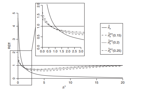
Consider the REff of $\hat{\theta}{n}^{\mathrm{pT}}(\alpha)$ compared to $\tilde{\theta}{n^{*}}$ Denoting it by REff $\left(\alpha ; \Delta^{2}\right)$, we have
$$
\operatorname{REff}\left(\alpha, \Delta^{2}\right)=\left[1+g\left(\Delta^{2}\right)\right]^{-1},
$$
where
$$
\begin{aligned}
g\left(\Delta^{2}\right)=&-\frac{\bar{x}^{2}}{Q}\left(\frac{1}{n}+\frac{\bar{x}^{2}}{Q}\right)^{-1}\left[G_{3, m}\left(\frac{1}{3} F_{1, m}(\alpha) ; \Delta^{2}\right)\right.\
&\left.-\Delta^{2}\left{2 G_{3, m}\left(\frac{1}{3} F_{1, m}(\alpha) ; \Delta^{2}\right)-G_{5, m}\left(\frac{1}{5} F_{1, m}(\alpha) ; \Delta^{2}\right)\right}\right]
\end{aligned}
$$
The graph of REff $\left(\alpha, \Delta^{2}\right)$, as a function of $\Delta^{2}$ for fixed $\alpha$, is decreasing crossing the 1-line to a minimum at $\Delta^{2}=\Delta_{0}^{2}(\alpha)$ (say); then it increases toward the 1-line as $\Delta^{2} \rightarrow \infty$. The maximum value of $\operatorname{REff}\left(\alpha, \Delta^{2}\right)$ occurs at $\Delta^{2}=0$ with the value
$$
\operatorname{REff}(\alpha ; 0)=\left{1-\frac{\bar{x}^{2}}{Q}\left(\frac{1}{n}+\frac{\bar{x}^{2}}{Q}\right)^{-1} G_{3, m}\left(\frac{1}{3} F_{1, m}(\alpha) ; 0\right)\right}^{-1} \geq 1,
$$
for all $\alpha \in A$, the set of possible values of $\alpha$. The value of REff $(\alpha ; 0)$ decreases as $\alpha$-values increase. On the other hand, if $\alpha=0$ and $\Delta^{2}$ vary, the graphs of $\operatorname{REff}\left(0, \Delta^{2}\right)$ and $\operatorname{REff}\left(1, \Delta^{2}\right)$ intersect at $\Delta^{2}=1$. In general, $\operatorname{REff}\left(\alpha_{1}, \Delta^{2}\right)$ and $\operatorname{REff}\left(\alpha_{2}, \Delta^{2}\right)$ intersect within the interval $0 \leq \Delta^{2} \leq 1$; the value of $\Delta^{2}$ at the intersection increases as $\alpha$-values increase. Therefore, for two different $\alpha$-values, $\operatorname{REff}\left(\alpha_{1}, \Delta^{2}\right)$ and $\operatorname{REff}\left(\alpha_{2}, \Delta^{2}\right)$ will always intersect below the 1 -line.
In order to obtain a PTE with a minimum guaranteed efficiency, $E_{0}$, we adopt the following procedure: If $0 \leq \Delta^{2} \leq 1$, we always choose $\tilde{\theta}{n}$, since $\operatorname{REff}\left(\alpha, \Delta^{2}\right) \geq 1$ in this interval. However, since in general $\Delta^{2}$ is unknown, there is no way to choose an estimate that is uniformly best. For this reason, we select an estimator with minimum guaranteed efficiency, such as $E{0}$, and look for a suitable $\alpha$ from the set, $A=\left{\alpha \mid \operatorname{REff}\left(\alpha, \Delta^{2}\right) \geq E_{0}\right}$. The estimator chosen

maximizes $\operatorname{REff}\left(\alpha, \Delta^{2}\right)$ over all $\alpha \in A$ and $\Delta^{2}$. Thus, we solve the following equation for the optimum $\alpha^{}$ : $$ \min {\Delta^{2}} \operatorname{REff}\left(\alpha, \Delta^{2}\right)=E\left(\alpha, \Delta{0}^{2}(\alpha)\right)=E_{0} .
$$
The solution $\alpha^{}$ obtained this way gives the PTE with minimum guaranteed efficiency $E_{0}$, which may increase toward $\operatorname{REff}\left(\alpha^{*}, 0\right)$ given by $(2.61)$, and Table $2.2$. For the following given data, we have computed the maximum and minimum guaranteed REff for the estimators of $\theta$ and provided them in Table 2.2.
$$
\begin{aligned}
x=&(19.383,21.117,18.99,19.415,20.394,20.212,20.163,20.521,20.125,\
& 19.944,18.345,21.45,19.479,20.199,20.677,19.661,20.114,19.724 \
&18.225,20.669)^{\top}
\end{aligned}
$$

似然估计代考

统计代写|似然估计作业代写Probability and Estimation代考|Comparison of Bias and MSE Functions

由于我们知道偏差和 MSE 表达式，我们可以将它们与三个估计量进行比较，即，θ~n,θ^n， 和θ^n磷吨(一种)也b~n,b^n， 和b^n磷吨(一种). 请注意，所有表达式都是Δ2，这是非中心的非中心参数F-分配。还，Δ2是之间的标准化距离b和b这. 首先，我们比较定理中的偏置函数2.4， 什么时候σ2是未知的。
为了X¯=0或以下H这,b(θ~n)=b(θ^n)=b(θ^np吨(一种))=0 b(b~n)=b(b^n)=b(b^n磷吨(一种))=0.

否则，对于所有Δ2和X¯≠0,
0=b(θ~n)≤|b(θ^np吨(一种))|=|b−b这|X¯3,米(13F1,米(一种);Δ2)≤|b(θ^n)| 0=b(b~n)≤|b(b^np吨(一种))|=|b−b这|G3,米(13F1,米(一种);Δ2)≤|b(b^n)|.绝对偏差θ^n是线性的Δ2，而绝对偏差θ^np吨(一种)增加到最大值Δ2远离原点，然后随着Δ2→∞. 类似的结论适用于b^n磷吨(一种).

现在，我们将受限估计器和 PTE 的 MSE 函数与传统估计器 $\tilde{\theta} {n}进行比较一种nd\波浪号 {\ beta} {n},r和sp和C吨一世在和l是.吨H和R和FF这F\hat{\theta} {n}$ 相比θ~n可以写成
REff⁡(θ^n:θ~n)=(1+nX¯2问)[1+nX¯2问Δ2]−1. 
效率是一个减函数Δ2. 在下面H这（IEΔ2=0)，它有最大值REff⁡(θ^n;θ~n)=(1+nX¯2问)≥1,和REff⁡(θ^n;θ~n)≥1，因此，如Δ2≥1. 因此，θ^n表现优于θ~n每当Δ2<1; 除此以外，θ~n表现更好θ^n. 的 REFFθ^np吨(一种)相比θ~n可以写成REff⁡(θ^n磷吨(一种);θ~n)=[1+G(Δ2)]−1,在哪里\begin{aligned} g\left(\Delta^{2}\right)=&-\frac{\bar{x}^{2}}{Q}\left(\frac{1}{n}+\ frac{\bar{x}^{2}}{Q}\right)^{-1}\left[G{3, m}\left(\frac{1}{3} F_{1, m}( \alpha) ; \Delta^{2}\right)\right.\ &\left.-\Delta^{2}\left{2 G_{3, m}\left(\frac{1}{3} F_ {1, m}(\alpha) ; \Delta^{2}\right)-G_{5, m}\left(\frac{1}{5} F_{1, m}(\alpha) ; \Delta ^{2}\right)\right}\right] \end{对齐}\begin{aligned} g\left(\Delta^{2}\right)=&-\frac{\bar{x}^{2}}{Q}\left(\frac{1}{n}+\ frac{\bar{x}^{2}}{Q}\right)^{-1}\left[G{3, m}\left(\frac{1}{3} F_{1, m}( \alpha) ; \Delta^{2}\right)\right.\ &\left.-\Delta^{2}\left{2 G_{3, m}\left(\frac{1}{3} F_ {1, m}(\alpha) ; \Delta^{2}\right)-G_{5, m}\left(\frac{1}{5} F_{1, m}(\alpha) ; \Delta ^{2}\right)\right}\right] \end{对齐}
在下面H0, 有最大值\operatorname{REff}\left(\hat{\theta}{n}^{\mathrm{pT}}(\alpha) ; \tilde{\theta}{n}\right)=\left{1-\frac {\bar{x}^{2}}{Q}\left(\frac{1}{n}+\frac{\bar{x}^{2}}{Q}\right)^{-1} G{3, m}\left(\frac{1}{3} F_{1, m}(\alpha) ; 0\right)\right}^{-1} \geq 1\operatorname{REff}\left(\hat{\theta}{n}^{\mathrm{pT}}(\alpha) ; \tilde{\theta}{n}\right)=\left{1-\frac {\bar{x}^{2}}{Q}\left(\frac{1}{n}+\frac{\bar{x}^{2}}{Q}\right)^{-1} G{3, m}\left(\frac{1}{3} F_{1, m}(\alpha) ; 0\right)\right}^{-1} \geq 1
和REff⁡(θ^np吨(一种);θ¨n)根据为
Δ2≤Δ2(一种)=G3,米(13F1,米(一种);Δ2)2G3,米(13F1,米(一种);Δ2)−G5,米(15F1,米(一种);Δ2)

统计代写|似然估计作业代写Probability and Estimation代考|Alternative PTE

在本小节中，我们提供了 PT 估计量及其偏差和 MSE 的替代表达式。检验假设H0:b=0对比H一种:b≠0，我们使用以下检验统计量：
从n=问b~nσ.的PTEb是（谁）给的b^n磷吨(一种)=b~n−b~n一世(|b~n|<λσ问) =σ问[从n−从n一世(|从n|<λ)]
在哪里λ=2日志⁡2.
因此，偏向于b~n等于b[披(λ−Δ)−披(−λ−Δ)]−[φ(λ−Δ)−φ(λ+ Δ), MSE 由下式给出MSE⁡(b^n磷吨)=σ2问ρ磷吨(λ,Δ)

统计代写|似然估计作业代写Probability and Estimation代考|Optimum Level of Significance of Preliminary Test

考虑 REffθ^np吨(一种)相比θ~n∗用 REff 表示(一种;Δ2)， 我们有
REff⁡(一种,Δ2)=[1+G(Δ2)]−1,
在哪里
\begin{aligned} g\left(\Delta^{2}\right)=&-\frac{\bar{x}^{2}}{Q}\left(\frac{1}{n}+\ frac{\bar{x}^{2}}{Q}\right)^{-1}\left[G_{3, m}\left(\frac{1}{3} F_{1, m}( \alpha) ; \Delta^{2}\right)\right.\ &\left.-\Delta^{2}\left{2 G_{3, m}\left(\frac{1}{3} F_ {1, m}(\alpha) ; \Delta^{2}\right)-G_{5, m}\left(\frac{1}{5} F_{1, m}(\alpha) ; \Delta ^{2}\right)\right}\right] \end{对齐}\begin{aligned} g\left(\Delta^{2}\right)=&-\frac{\bar{x}^{2}}{Q}\left(\frac{1}{n}+\ frac{\bar{x}^{2}}{Q}\right)^{-1}\left[G_{3, m}\left(\frac{1}{3} F_{1, m}( \alpha) ; \Delta^{2}\right)\right.\ &\left.-\Delta^{2}\left{2 G_{3, m}\left(\frac{1}{3} F_ {1, m}(\alpha) ; \Delta^{2}\right)-G_{5, m}\left(\frac{1}{5} F_{1, m}(\alpha) ; \Delta ^{2}\right)\right}\right] \end{对齐}
REff 的图表(一种,Δ2), 作为一个函数Δ2对于固定一种, 越过 1 线减少到最小值Δ2=Δ02(一种)（说）; 然后它向 1 线增加Δ2→∞. 的最大值REff⁡(一种,Δ2)发生在Δ2=0与价值
\operatorname{REff}(\alpha ; 0)=\left{1-\frac{\bar{x}^{2}}{Q}\left(\frac{1}{n}+\frac{\bar {x}^{2}}{Q}\right)^{-1} G_{3, m}\left(\frac{1}{3} F_{1, m}(\alpha) ; 0\right )\right}^{-1} \geq 1,\operatorname{REff}(\alpha ; 0)=\left{1-\frac{\bar{x}^{2}}{Q}\left(\frac{1}{n}+\frac{\bar {x}^{2}}{Q}\right)^{-1} G_{3, m}\left(\frac{1}{3} F_{1, m}(\alpha) ; 0\right )\right}^{-1} \geq 1,
对全部一种∈一种, 的可能值的集合一种. REff 的值(一种;0)减少为一种-值增加。另一方面，如果一种=0和Δ2变化，图表REff⁡(0,Δ2)和REff⁡(1,Δ2)相交于Δ2=1. 一般来说，REff⁡(一种1,Δ2)和REff⁡(一种2,Δ2)在区间内相交0≤Δ2≤1; 的价值Δ2在交叉点处增加为一种-值增加。因此，对于两个不同的一种-价值观，REff⁡(一种1,Δ2)和REff⁡(一种2,Δ2)将始终在 1 线下方相交。
为了获得具有最低保证效率的 PTE，和0，我们采用以下程序：如果0≤Δ2≤1，我们总是选择θ~n， 自从REff⁡(一种,Δ2)≥1在这个区间。然而，由于一般Δ2是未知的，没有办法选择一致最佳的估计。因此，我们选择保证效率最低的估计器，例如和0，并寻找合适的一种从集合中，A=\left{\alpha \mid \operatorname{REff}\left(\alpha, \Delta^{2}\right) \geq E_{0}\right}A=\left{\alpha \mid \operatorname{REff}\left(\alpha, \Delta^{2}\right) \geq E_{0}\right}. 选择的估计器

最大化REff⁡(一种,Δ2)总体一种∈一种和Δ2. 因此，我们求解以下方程以获得最佳一种 :分钟Δ2REff⁡(一种,Δ2)=和(一种,Δ02(一种))=和0.
解决方案一种以这种方式获得的 PTE 具有最低的保证效率和0, 这可能会增加REff⁡(一种∗,0)由(2.61), 和表2.2. 对于以下给定数据，我们计算了估计量的最大和最小保证 REffθ并在表 2.2 中提供。
X=(19.383,21.117,18.99,19.415,20.394,20.212,20.163,20.521,20.125, 19.944,18.345,21.45,19.479,20.199,20.677,19.661,20.114,19.724 18.225,20.669)⊤

统计代写请认准statistics-lab™. statistics-lab™为您的留学生涯保驾护航。

金融工程代写

金融工程是使用数学技术来解决金融问题。金融工程使用计算机科学、统计学、经济学和应用数学领域的工具和知识来解决当前的金融问题，以及设计新的和创新的金融产品。

非参数统计代写

非参数统计指的是一种统计方法，其中不假设数据来自于由少数参数决定的规定模型；这种模型的例子包括正态分布模型和线性回归模型。

广义线性模型代考

广义线性模型（GLM）归属统计学领域，是一种应用灵活的线性回归模型。该模型允许因变量的偏差分布有除了正态分布之外的其它分布。

术语 广义线性模型（GLM）通常是指给定连续和/或分类预测因素的连续响应变量的常规线性回归模型。它包括多元线性回归，以及方差分析和方差分析（仅含固定效应）。

有限元方法代写

有限元方法（FEM）是一种流行的方法，用于数值解决工程和数学建模中出现的微分方程。典型的问题领域包括结构分析、传热、流体流动、质量运输和电磁势等传统领域。

有限元是一种通用的数值方法，用于解决两个或三个空间变量的偏微分方程（即一些边界值问题）。为了解决一个问题，有限元将一个大系统细分为更小、更简单的部分，称为有限元。这是通过在空间维度上的特定空间离散化来实现的，它是通过构建对象的网格来实现的：用于求解的数值域，它有有限数量的点。边界值问题的有限元方法表述最终导致一个代数方程组。该方法在域上对未知函数进行逼近。[1] 然后将模拟这些有限元的简单方程组合成一个更大的方程系统，以模拟整个问题。然后，有限元通过变化微积分使相关的误差函数最小化来逼近一个解决方案。

tatistics-lab作为专业的留学生服务机构，多年来已为美国、英国、加拿大、澳洲等留学热门地的学生提供专业的学术服务，包括但不限于Essay代写，Assignment代写，Dissertation代写，Report代写，小组作业代写，Proposal代写，Paper代写，Presentation代写，计算机作业代写，论文修改和润色，网课代做，exam代考等等。写作范围涵盖高中，本科，研究生等海外留学全阶段，辐射金融，经济学，会计学，审计学，管理学等全球99%专业科目。写作团队既有专业英语母语作者，也有海外名校硕博留学生，每位写作老师都拥有过硬的语言能力，专业的学科背景和学术写作经验。我们承诺100%原创，100%专业，100%准时，100%满意。

随机分析代写

随机微积分是数学的一个分支，对随机过程进行操作。它允许为随机过程的积分定义一个关于随机过程的一致的积分理论。这个领域是由日本数学家伊藤清在第二次世界大战期间创建并开始的。

时间序列分析代写

随机过程，是依赖于参数的一组随机变量的全体，参数通常是时间。 随机变量是随机现象的数量表现，其时间序列是一组按照时间发生先后顺序进行排列的数据点序列。通常一组时间序列的时间间隔为一恒定值（如1秒，5分钟，12小时，7天，1年），因此时间序列可以作为离散时间数据进行分析处理。研究时间序列数据的意义在于现实中，往往需要研究某个事物其随时间发展变化的规律。这就需要通过研究该事物过去发展的历史记录，以得到其自身发展的规律。

回归分析代写

多元回归分析渐进（Multiple Regression Analysis Asymptotics）属于计量经济学领域，主要是一种数学上的统计分析方法，可以分析复杂情况下各影响因素的数学关系，在自然科学、社会和经济学等多个领域内应用广泛。

MATLAB代写

MATLAB 是一种用于技术计算的高性能语言。它将计算、可视化和编程集成在一个易于使用的环境中，其中问题和解决方案以熟悉的数学符号表示。典型用途包括：数学和计算算法开发建模、仿真和原型制作数据分析、探索和可视化科学和工程图形应用程序开发，包括图形用户界面构建MATLAB 是一个交互式系统，其基本数据元素是一个不需要维度的数组。这使您可以解决许多技术计算问题，尤其是那些具有矩阵和向量公式的问题，而只需用 C 或 Fortran 等标量非交互式语言编写程序所需的时间的一小部分。MATLAB 名称代表矩阵实验室。MATLAB 最初的编写目的是提供对由 LINPACK 和 EISPACK 项目开发的矩阵软件的轻松访问，这两个项目共同代表了矩阵计算软件的最新技术。MATLAB 经过多年的发展，得到了许多用户的投入。在大学环境中，它是数学、工程和科学入门和高级课程的标准教学工具。在工业领域，MATLAB 是高效研究、开发和分析的首选工具。MATLAB 具有一系列称为工具箱的特定于应用程序的解决方案。对于大多数 MATLAB 用户来说非常重要，工具箱允许您学习和应用专业技术。工具箱是 MATLAB 函数（M 文件）的综合集合，可扩展 MATLAB 环境以解决特定类别的问题。可用工具箱的领域包括信号处理、控制系统、神经网络、模糊逻辑、小波、仿真等。

R语言代写	问卷设计与分析代写
PYTHON代写	回归分析与线性模型代写
MATLAB代写	方差分析与试验设计代写
STATA代写	机器学习/统计学习代写
SPSS代写	计量经济学代写
EVIEWS代写	时间序列分析代写
EXCEL代写	深度学习代写
SQL代写	各种数据建模与可视化代写

如果你也在 怎样代写似然估计Probability and Estimation这个学科遇到相关的难题，请随时右上角联系我们的24/7代写客服。

似然估计是一种统计方法，它用来求一个样本集的相关概率密度函数的参数。

statistics-lab™ 为您的留学生涯保驾护航 在代写似然估计Probability and Estimation方面已经树立了自己的口碑, 保证靠谱, 高质且原创的统计Statistics代写服务。我们的专家在代写似然估计Probability and Estimation代写方面经验极为丰富，各种代写似然估计Probability and Estimation相关的作业也就用不着说。

我们提供的似然估计Probability and Estimation及其相关学科的代写，服务范围广, 其中包括但不限于:

• Statistical Inference 统计推断
• Statistical Computing 统计计算
• Advanced Probability Theory 高等楖率论
• Advanced Mathematical Statistics 高等数理统计学
• (Generalized) Linear Models 广义线性模型
• Statistical Machine Learning 统计机器学习
• Longitudinal Data Analysis 纵向数据分析
• Foundations of Data Science 数据科学基础

统计代写|似然估计作业代写Probability and Estimation代考|Estimation of the Intercept and Slope Parameters

First, we consider the LSE of the parameters. Using the model $(2.1)$ and the sample information from the normal distribution, we obtain the LSEs of $(\theta, \beta)^{\top}$ as
$$
\left(\begin{array}{c}
\tilde{\theta}{n} \ \tilde{\beta}{n}
\end{array}\right)=\left(\begin{array}{c}
\bar{y}-\tilde{\beta}{n} \bar{x} \ \frac{1}{Q}\left[x^{\top} \boldsymbol{Y}-\frac{1}{n}\left(\mathbf{1}{n}^{\top} \boldsymbol{x}\right)\left(\mathbf{1}_{n}^{\top} \boldsymbol{Y}\right)\right]
\end{array}\right)
$$

where
$$
\bar{x}=\frac{1}{n} \mathbf{1}{n}^{\top} \boldsymbol{x}, \quad \bar{y}=\frac{1}{n} \mathbf{1}{n}^{\top} Y, \quad Q=\boldsymbol{x}^{\top} \boldsymbol{x}-\frac{1}{n}\left(\mathbf{1}{n}^{\top} \boldsymbol{x}\right)^{2} . $$ The exact distribution of $\left(\tilde{\theta}{n}, \tilde{\beta}{n}\right)^{\top}$ is a bivariate normal with mean $(\theta, \beta)^{\top}$ and covariance matrix $$ \frac{\sigma^{2}}{n}\left(\begin{array}{cc} 1+\frac{n \bar{x}^{2}}{Q} & -\frac{n \bar{x}}{Q} \ \frac{n \bar{x}}{Q} & \frac{n}{Q} \end{array}\right) $$ An unbiased estimator of the variance $\sigma^{2}$ is given by $$ s{n}^{2}=(n-2)^{-1}\left(\boldsymbol{Y}-\tilde{\theta}{n} \mathbf{1}{n}-\tilde{\beta}{n} \boldsymbol{x}\right)^{\top}\left(\boldsymbol{Y}-\tilde{\theta}{n} \mathbf{1}{n}-\tilde{\beta}{n} \boldsymbol{x}\right),
$$
which is independent of $\left(\tilde{\theta}{n}, \tilde{\beta}{n}\right)$, and $(n-2) s_{n}^{2} / \sigma^{2}$ follows a central chi-square distribution with ( $n-2$ ) degrees of freedom (DF)

统计代写|似然估计作业代写Probability and Estimation代考|Test for Slope Parameter

Suppose that we want to test the null-hypothesis $\mathcal{H}{0}: \beta=\beta{o}$ vs. $\mathcal{H}{A}: \beta \neq \beta{o}$. Then, we use the likelihood ratio (LR) test statistic
$\mathcal{L}{n}^{(\sigma)}=\frac{\left(\tilde{\beta}{n}-\beta_{\mathrm{o}}\right)^{2} Q}{\sigma^{2}}, \quad$ if $\sigma^{2}$ is known
$\mathcal{L}{n}^{(s)}=\frac{\left(\tilde{\beta}{n}-\beta_{\mathrm{o}}\right)^{2} Q}{s_{n}^{2}}, \quad$ if $\sigma^{2}$ is unknown
where $\mathcal{L}{n}^{(\sigma)}$ follows a noncentral chi-square distribution with $1 \mathrm{DF}$ and noncentrality parameter $\Delta^{2} / 2$ and $\mathcal{L}{n}^{(s)}$ follows a noncentral $F$-distribution with $(1, m)$, where $m=n-2$ is DF and also the noncentral parameter is
$$
\Delta^{2}=\frac{\left(\beta-\beta_{\mathrm{o}}\right)^{2} Q}{\sigma^{2}}
$$
Under $\mathcal{H}{\mathrm{o}}, \mathcal{L}{n}^{(\sigma)}$ follows a central chi-square distribution and $\mathcal{L}{n}^{(s)}$ follows a central $F$-distribution. At the $\alpha$-level of significance, we obtain the critical value $\chi{1}^{2}(\alpha)$ or $F_{1, m}(\alpha)$ from the distribution and reject $\mathcal{H}{0}$ if $\mathcal{L}{n}^{(\sigma)}>\chi_{1}^{2}(\alpha)$ or $\mathcal{L}{n}^{(s)}>$ $F{1, n}(\alpha)$; otherwise, we accept $\mathcal{H}_{\mathrm{o}^{*}}$

统计代写|似然估计作业代写Probability and Estimation代考|PTE of the Intercept and Slope Parameters

This section deals with the problem of estimation of the intercept and slope parameters $(\theta, \beta)$ when it is suspected that the slope parameter $\beta$ may be $\beta_{o^{\circ}}$ From (2.30), we know that the LSE of $\theta$ is given by
$$
\tilde{\theta}{n}=\bar{y}-\tilde{\beta}{n} \bar{x} .
$$

If we know $\beta$ to be $\beta_{0}$ exactly, then the restricted least squares estimator (RLSE) of $\theta$ is given by
$$
\hat{\theta}{n}=\bar{y}-\beta{\mathrm{o}} \bar{x} .
$$
In practice, the prior information that $\beta=\beta_{\mathrm{o}}$ is uncertain. The doubt regarding this prior information can be removed using Fisher’s recipe of testing the null-hypothesis $\mathcal{H}{o}: \beta=\beta{o}$ against the alternative $\mathcal{H}{A}: \beta \neq \beta{o}$. As a result of this test, we choose $\tilde{\theta}{n}$ or $\hat{\theta}{n}$ based on the rejection or acceptance of $\mathcal{H}{\mathrm{a}}$. Accordingly, in case of the unknown variance, we write the estimator as $$ \hat{\theta}{n}^{\mathrm{PT}}(\alpha)=\hat{\theta}{n} I\left(\mathcal{L}{n}^{(s)} \leq F_{1, m}(\alpha)\right)+\tilde{\theta}{n} I\left(\mathcal{L}{n}^{(s)}>F_{1, m}(\alpha)\right), \quad m=n-2
$$
called the PTE, where $F_{1, n}(\alpha)$ is the $\alpha$-level upper critical value of a central $F$-distribution with $(1, m)$ DF and $I(A)$ is the indicator function of the set $A$. For more details on PTE, see Saleh (2006), Ahmed and Saleh (1988), Ahsanullah and Saleh (1972), Kibria and Saleh (2012) and, recently Saleh et al. (2014), among others. We can write PTE of $\theta$ as
$$
\hat{\theta}{n}^{\mathrm{pT}}(\alpha)=\tilde{\theta}{n}+\left(\tilde{\beta}{n}-\beta{\mathrm{o}}\right) \bar{x} I\left(\mathcal{L}{n}^{(s)} \leq F{1, m}(\alpha)\right), \quad m=n-2
$$
If $\alpha=1, \tilde{\theta}{n}$ is always chosen; and if $\alpha=0, \hat{\theta}{n}$ is chosen. Since $0<\alpha<1$, $\hat{\theta}{n}^{\mathrm{pT}}(\alpha)$ in repeated samples, this will result in a combination of $\tilde{\theta}{n}$ and $\hat{\theta}{n}$. Note that the PTE procedure leads to the choice of one of the two values, namely, either $\dot{\theta}{n}$ or $\hat{\theta}_{n}$. Also, the PTE procedure depends on the level of significance $\alpha$.

Clearly, $\hat{\beta}{n}$ is the unrestricted estimator of $\beta$, while $\beta{\mathrm{o}}$ is the restricted estimator. Thus, the PTE of $\beta$ is given by
$$
\hat{\beta}{n}^{P \mathrm{~T}}(\alpha)=\tilde{\beta}{n}-\left(\tilde{\beta}{a}-\beta{\mathrm{o}}\right) I\left(\mathcal{L}{n}^{(s)} \leq F{1, m}(\alpha)\right), \quad m=n-2 .
$$
Now, if $\alpha=1, \tilde{\beta}{n}$ is always chosen; and if $\alpha=0, \beta{\mathrm{o}}$ is always chosen.
Since our interest is to compare the LSE, RLSE, and PTE of $\theta$ and $\beta$ with respect to bias and the MSE, we obtain the expression of these quantities in the following theorem. First we consider the bias expressions of the estimators.

似然估计代考

统计代写|似然估计作业代写Probability and Estimation代考|Estimation of the Intercept and Slope Parameters

首先，我们考虑参数的 LSE。使用模型(2.1)和来自正态分布的样本信息，我们得到 LSE(θ,b)⊤作为
(θ~n b~n)=(是¯−b~nX¯ 1问[X⊤是−1n(1n⊤X)(1n⊤是)])

在哪里
X¯=1n1n⊤X,是¯=1n1n⊤是,问=X⊤X−1n(1n⊤X)2.的准确分布(θ~n,b~n)⊤是具有均值的双变量正态(θ,b)⊤和协方差矩阵σ2n(1+nX¯2问−nX¯问 nX¯问n问)方差的无偏估计σ2是（谁）给的sn2=(n−2)−1(是−θ~n1n−b~nX)⊤(是−θ~n1n−b~nX),
它独立于 $\left(\tilde{\theta} {n}, \tilde{\beta} {n}\right),一种nd(n-2) s_{n}^{2} / \sigma^{2}F这ll这在s一种C和n吨r一种lCH一世−sq在一种r和d一世s吨r一世b在吨一世这n在一世吨H(n-2$ ) 自由度 (DF)

统计代写|似然估计作业代写Probability and Estimation代考|Test for Slope Parameter

假设我们要检验零假设H0:b=b这对比H一种:b≠b这. 然后，我们使用似然比（LR）检验统计量
大号n(σ)=(b~n−b这)2问σ2,如果σ2已知
大号n(s)=(b~n−b这)2问sn2,如果σ2不知道
在哪里大号n(σ)遵循非中心卡方分布1DF和非中心性参数Δ2/2和大号n(s)遵循非中心F-分布与(1,米)， 在哪里米=n−2是 DF 并且非中心参数是
Δ2=(b−b这)2问σ2
在下面H这,大号n(σ)遵循中心卡方分布和大号n(s)遵循中央F-分配。在一种-显着性水平，我们获得临界值χ12(一种)或者F1,米(一种)从分配和拒绝H0如果大号n(σ)>χ12(一种)或者大号n(s)> F1,n(一种); 否则，我们接受H这∗

统计代写|似然估计作业代写Probability and Estimation代考|PTE of the Intercept and Slope Parameters

本节处理截距和斜率参数的估计问题(θ,b)当怀疑斜率参数b或许b这∘从 (2.30)，我们知道 LSEθ是（谁）给的
θ~n=是¯−b~nX¯.

如果我们知道b成为b0确切地说，那么受限最小二乘估计量 (RLSE)θ是（谁）给的
θ^n=是¯−b这X¯.
在实践中，先验信息b=b这是不确定的。可以使用 Fisher 的零假设检验方法来消除对这些先验信息的怀疑H这:b=b这反对替代方案H一种:b≠b这. 作为这个测试的结果，我们选择θ~n或者θ^n基于拒绝或接受H一种. 因此，在未知方差的情况下，我们将估计量写为θ^n磷吨(一种)=θ^n一世(大号n(s)≤F1,米(一种))+θ~n一世(大号n(s)>F1,米(一种)),米=n−2
称为 PTE，其中F1,n(一种)是个一种一个中心的级上临界值F-分布与(1,米)东风和一世(一种)是集合的指示函数一种. 有关 PTE 的更多详细信息，请参见 Saleh (2006)、Ahmed 和 Saleh (1988)、Ahsanullah 和 Saleh (1972)、Kibria 和 Saleh (2012)，以及最近的 Saleh 等人。（2014 年）等。我们可以写PTEθ作为
θ^np吨(一种)=θ~n+(b~n−b这)X¯一世(大号n(s)≤F1,米(一种)),米=n−2
如果一种=1,θ~n总是被选中；而如果一种=0,θ^n被选中。自从0<一种<1, θ^np吨(一种)在重复的样本中，这将导致θ~n和θ^n. 请注意，PTE 过程导致选择两个值之一，即θ˙n或者θ^n. 此外，PTE 程序取决于显着性水平一种.

清楚地，b^n是的无限制估计量b， 尽管b这是受限估计量。因此，PTEb是（谁）给的
b^n磷 吨(一种)=b~n−(b~一种−b这)一世(大号n(s)≤F1,米(一种)),米=n−2.
现在，如果一种=1,b~n总是被选中；而如果一种=0,b这总是被选中。
因为我们的兴趣是比较 LSE、RLSE 和 PTEθ和b关于偏差和 MSE，我们在以下定理中获得了这些量的表达式。首先，我们考虑估计量的偏差表达式。

统计代写请认准statistics-lab™. statistics-lab™为您的留学生涯保驾护航。

金融工程代写

金融工程是使用数学技术来解决金融问题。金融工程使用计算机科学、统计学、经济学和应用数学领域的工具和知识来解决当前的金融问题，以及设计新的和创新的金融产品。

非参数统计代写

非参数统计指的是一种统计方法，其中不假设数据来自于由少数参数决定的规定模型；这种模型的例子包括正态分布模型和线性回归模型。

广义线性模型代考

广义线性模型（GLM）归属统计学领域，是一种应用灵活的线性回归模型。该模型允许因变量的偏差分布有除了正态分布之外的其它分布。

术语 广义线性模型（GLM）通常是指给定连续和/或分类预测因素的连续响应变量的常规线性回归模型。它包括多元线性回归，以及方差分析和方差分析（仅含固定效应）。

有限元方法代写

有限元方法（FEM）是一种流行的方法，用于数值解决工程和数学建模中出现的微分方程。典型的问题领域包括结构分析、传热、流体流动、质量运输和电磁势等传统领域。

有限元是一种通用的数值方法，用于解决两个或三个空间变量的偏微分方程（即一些边界值问题）。为了解决一个问题，有限元将一个大系统细分为更小、更简单的部分，称为有限元。这是通过在空间维度上的特定空间离散化来实现的，它是通过构建对象的网格来实现的：用于求解的数值域，它有有限数量的点。边界值问题的有限元方法表述最终导致一个代数方程组。该方法在域上对未知函数进行逼近。[1] 然后将模拟这些有限元的简单方程组合成一个更大的方程系统，以模拟整个问题。然后，有限元通过变化微积分使相关的误差函数最小化来逼近一个解决方案。

tatistics-lab作为专业的留学生服务机构，多年来已为美国、英国、加拿大、澳洲等留学热门地的学生提供专业的学术服务，包括但不限于Essay代写，Assignment代写，Dissertation代写，Report代写，小组作业代写，Proposal代写，Paper代写，Presentation代写，计算机作业代写，论文修改和润色，网课代做，exam代考等等。写作范围涵盖高中，本科，研究生等海外留学全阶段，辐射金融，经济学，会计学，审计学，管理学等全球99%专业科目。写作团队既有专业英语母语作者，也有海外名校硕博留学生，每位写作老师都拥有过硬的语言能力，专业的学科背景和学术写作经验。我们承诺100%原创，100%专业，100%准时，100%满意。

随机分析代写

随机微积分是数学的一个分支，对随机过程进行操作。它允许为随机过程的积分定义一个关于随机过程的一致的积分理论。这个领域是由日本数学家伊藤清在第二次世界大战期间创建并开始的。

时间序列分析代写

随机过程，是依赖于参数的一组随机变量的全体，参数通常是时间。 随机变量是随机现象的数量表现，其时间序列是一组按照时间发生先后顺序进行排列的数据点序列。通常一组时间序列的时间间隔为一恒定值（如1秒，5分钟，12小时，7天，1年），因此时间序列可以作为离散时间数据进行分析处理。研究时间序列数据的意义在于现实中，往往需要研究某个事物其随时间发展变化的规律。这就需要通过研究该事物过去发展的历史记录，以得到其自身发展的规律。

回归分析代写

多元回归分析渐进（Multiple Regression Analysis Asymptotics）属于计量经济学领域，主要是一种数学上的统计分析方法，可以分析复杂情况下各影响因素的数学关系，在自然科学、社会和经济学等多个领域内应用广泛。

MATLAB代写

MATLAB 是一种用于技术计算的高性能语言。它将计算、可视化和编程集成在一个易于使用的环境中，其中问题和解决方案以熟悉的数学符号表示。典型用途包括：数学和计算算法开发建模、仿真和原型制作数据分析、探索和可视化科学和工程图形应用程序开发，包括图形用户界面构建MATLAB 是一个交互式系统，其基本数据元素是一个不需要维度的数组。这使您可以解决许多技术计算问题，尤其是那些具有矩阵和向量公式的问题，而只需用 C 或 Fortran 等标量非交互式语言编写程序所需的时间的一小部分。MATLAB 名称代表矩阵实验室。MATLAB 最初的编写目的是提供对由 LINPACK 和 EISPACK 项目开发的矩阵软件的轻松访问，这两个项目共同代表了矩阵计算软件的最新技术。MATLAB 经过多年的发展，得到了许多用户的投入。在大学环境中，它是数学、工程和科学入门和高级课程的标准教学工具。在工业领域，MATLAB 是高效研究、开发和分析的首选工具。MATLAB 具有一系列称为工具箱的特定于应用程序的解决方案。对于大多数 MATLAB 用户来说非常重要，工具箱允许您学习和应用专业技术。工具箱是 MATLAB 函数（M 文件）的综合集合，可扩展 MATLAB 环境以解决特定类别的问题。可用工具箱的领域包括信号处理、控制系统、神经网络、模糊逻辑、小波、仿真等。

R语言代写	问卷设计与分析代写
PYTHON代写	回归分析与线性模型代写
MATLAB代写	方差分析与试验设计代写
STATA代写	机器学习/统计学习代写
SPSS代写	计量经济学代写
EVIEWS代写	时间序列分析代写
EXCEL代写	深度学习代写
SQL代写	各种数据建模与可视化代写