物理代写|广义相对论代写General relativity代考|Derivation of Hubble’s Law
如果你也在 怎样代写广义相对论General relativity这个学科遇到相关的难题,请随时右上角联系我们的24/7代写客服。
广义相对论是阿尔伯特-爱因斯坦在1907至1915年间提出的引力理论。广义相对论说,观察到的质量之间的引力效应是由它们对时空的扭曲造成的。
statistics-lab™ 为您的留学生涯保驾护航 在代写广义相对论General relativity方面已经树立了自己的口碑, 保证靠谱, 高质且原创的统计Statistics代写服务。我们的专家在代写广义相对论General relativity代写方面经验极为丰富,各种代写广义相对论General relativity相关的作业也就用不着说。
我们提供的广义相对论General relativity及其相关学科的代写,服务范围广, 其中包括但不限于:
- Statistical Inference 统计推断
- Statistical Computing 统计计算
- Advanced Probability Theory 高等概率论
- Advanced Mathematical Statistics 高等数理统计学
- (Generalized) Linear Models 广义线性模型
- Statistical Machine Learning 统计机器学习
- Longitudinal Data Analysis 纵向数据分析
- Foundations of Data Science 数据科学基础
物理代写|广义相对论代写General relativity代考|Derivation of Hubble’s Law
Consider a light ray propagation from a distant galaxy at $\left(r_1, \theta_1, \phi_1\right)$ towards $r=0$. The equations of a null geodesic imply that this light ray moves along the path $\theta=\theta_1, \phi=\phi_1$. Suppose the present epoch is denoted by $t=t_0$ and let a right ray leave the source at $t=t_1$. Then the condition for the ray to reach at $r=0$, at $t=t_0$
$$
\int_{t_1}^{t_0} \frac{c d t}{a(t)}=\int_0^{r_1} \frac{d r}{\sqrt{1-k r^2}}=f\left(r_1\right) .
$$
Assuming that $r_1$ is small for nearby objects, we then get approximately,
$$
f\left(r_1\right) \cong r_1 \cong \frac{c\left(t_0-t_1\right)}{a\left(t_0\right)}
$$
Now Taylor’s expansion near $t_0$,
$$
\begin{aligned}
a\left(t_1\right) & \cong a\left(t_0\right)+\left(t_1-t_0\right) \dot{a}\left(t_0\right)=a\left(t_0\right)\left[1-\left(t_0-t_1\right) \frac{\dot{a}\left(t_0\right)}{a\left(t_0\right)}\right], \
& =a\left(t_0\right)\left[1-\left(t_0-t_1\right) H_0\right] \text { where } H_0=\frac{\dot{a}\left(t_0\right)}{a\left(t_0\right)} .
\end{aligned}
$$
Also, we know
$$
(1+z)^{-1}=\frac{a\left(t_1\right)}{a\left(t_0\right)} \cong 1-\left(t_0-t_1\right) H_0 .
$$
For, small redshift $z$, we have
$$
1-z \cong 1-\left(t_0-t_1\right) H_0
$$
This implies
$$
\begin{gathered}
c z \cong r_1 a\left(t_0\right) H_0=D_1 H_0, \
\text { where } D_1=r_1 a\left(t_0\right),
\end{gathered}
$$
may be defined as a proper distance at the epoch $t_0$.
From a Doppler shift point of view, cz may be identified with the velocity of recession of a galaxy in proportion to its distance from us. This is Hubble’s law and $H_0$ is the Hubble’s constant given by
$$
H_0=\frac{\dot{a}\left(t_0\right)}{a\left(t_0\right)}
$$
物理代写|广义相对论代写General relativity代考|Angular Size
The angular measurement describing how a large sphere or circle looks from a given point of view is the angular diameter or angular size. In Euclidean geometry, the diameter $d$ is related to the observed angle $\Delta \theta$ as
$$
\Delta \theta=\frac{d}{r},
$$
where $r$ is its distance. However, for curved spacetime, one needs to use $\mathrm{R}-\mathrm{W}$ spacetime.
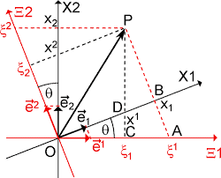
Let us consider a galaxy $G_1$ having linear extend $d(\overline{A B})$ and the angle subtended by this galaxy $G_1$ at the observer $\mathrm{O}$ is $\Delta \theta_1$ (see Fig. 101). Consider two neighboring null geodesics (representing light rays) from the two points $A, B$ at the two extremities of $G_1$. Without any loss of generality, we can select the coordinates of $A$ and $B$ as $\left(\theta_1, \phi_1\right)$ and $\left(\theta_1+\Delta \theta_1, \phi_1\right)$, respectively. For the curved space, we use R-W line element to find the proper distance between $A$ and $B$. Now, plugging $t=t_1=$ constant, $r=r_1=$ constant, $\phi=\phi_1=$ constant, and $d \theta=\Delta \theta_1$ in the R-W line element, we get
$$
d s^2=-r_1^2 a^2\left(t_1\right)\left(\Delta \theta_1\right)^2=-d^2
$$
[in $G_1$, the space-like separation $A B=d$, which is a rest frame] Thus,
$$
\begin{aligned}
\Delta \theta_1 & =\frac{d}{r_1 a\left(t_1\right)}=\frac{d(1+z)}{r_1 a\left(t_0\right)}, \quad \text { (using Eq. (11.30)) } \
& =\frac{d(1+z)}{D_1} .[\text { using Eq. (11.36)] }
\end{aligned}
$$
Note that in Euclidean space, $\Delta \theta_1$ is decreasing with an increase in the distance of the galaxy from us. However, in curved space, the result is different. For expanding universe, the scale factor $a(t)$ is increasing with time and consequently, $z$ will be increasing (by Eq. (11.31)). Therefore, it is not always true that $\Delta \theta_1$ decreases with time. Light from a galaxy takes much time to reach us for expanding universe.

广义相对论代考
物理代写|广义相对论代写General relativity代考|Derivation of Hubble’s Law
考虑来自遥远星系的光线传播 $\left(r_1, \theta_1, \phi_1\right)$ 向 $r=0$. 零测地线的方程意味着这条光线沿着路径移动 $\theta=\theta_1, \phi=\phi_1$. 假设当前纪元表示为 $t=t_0$ 并让右光线离开光源 $t=t_1$. 那么光线到达的条件是 $r=0$ , 在 $t=t_0$
$$
\int_{t_1}^{t_0} \frac{c d t}{a(t)}=\int_0^{r_1} \frac{d r}{\sqrt{1-k r^2}}=f\left(r_1\right)
$$
假如说 $r_1$ 对于附近的物体来说很小,然后我们得到大约,
$$
f\left(r_1\right) \cong r_1 \cong \frac{c\left(t_0-t_1\right)}{a\left(t_0\right)}
$$
现在泰勒的扩张临近 $t_0$ ,
$$
a\left(t_1\right) \cong a\left(t_0\right)+\left(t_1-t_0\right) \dot{a}\left(t_0\right)=a\left(t_0\right)\left[1-\left(t_0-t_1\right) \frac{\dot{a}\left(t_0\right)}{a\left(t_0\right)}\right], \quad=a\left(t_0\right)\left[1-\left(t_0-t_1\right) H_0\right]
$$
另外,我们知道
$$
(1+z)^{-1}=\frac{a\left(t_1\right)}{a\left(t_0\right)} \cong 1-\left(t_0-t_1\right) H_0
$$
对于,小红移 $z$ ,我们有
$$
1-z \cong 1-\left(t_0-t_1\right) H_0
$$
这意味着
$$
c z \cong r_1 a\left(t_0\right) H_0=D_1 H_0, \text { where } D_1=r_1 a\left(t_0\right),
$$
可以定义为纪元的适当距离 $t_0$.
从多普勒频移的角度来看, $c z$ 可以等同于星系的后退速度与其与我们的距离成正比。这是哈勃定律 $H_0$ 是哈勃 常数
$$
H_0=\frac{\dot{a}\left(t_0\right)}{a\left(t_0\right)}
$$
物理代写|广义相对论代写General relativity代考|Angular Size
描述大球体或圆从给定角度看起来如何的角度测量是角直径或角大小。在欧氏几何中,直径 $d$ 与观察角度有关 $\Delta \theta$ 作为
$$
\Delta \theta=\frac{d}{r}
$$
在哪里 $r$ 是它的距离。然而,对于弯曲时空,需要使用 $\mathrm{R}-\mathrm{W}$ 时空。
让我们考虑一个星系 $G_1$ 有线性延伸 $d(\overline{A B})$ 以及这个星系所夹的角度 $G_1$ 在观察者 $\mathrm{O}$ 是 $\Delta \theta_1$ (见图 101)。从 两个点考虑两个相邻的零测地线 (代表光线) $A, B$ 在两端 $G_1$. 不失一般性,我们可以选择坐标 $A$ 和 $B$ 作为 $\left(\theta_1, \phi_1\right)$ 和 $\left(\theta_1+\Delta \theta_1, \phi_1\right)$ , 分别。对于弯曲空间,我们使用RW线元来找到合适的距离 $A$ 和 $B$. 现在,堵 $t=t_1$ =持续的, $r=r_1=$ 持续的, $\phi=\phi_1=$ 常数,和 $d \theta=\Delta \theta_1$ 在 RW 行元素中,我们得到
$$
d s^2=-r_1^2 a^2\left(t_1\right)\left(\Delta \theta_1\right)^2=-d^2
$$
[在 $G_1$ ,类似空间的分离 $A B=d$ ,这是一个休息框架]因此,
$$
\Delta \theta_1=\frac{d}{r_1 a\left(t_1\right)}=\frac{d(1+z)}{r_1 a\left(t_0\right)}, \quad \text { (using Eq. (11.30)) } \quad=\frac{d(1+z)}{D_1} \cdot[\text { using Eq. (11.36)] }
$$
请注意,在欧几里德空间中, $\Delta \theta_1$ 随着银河系离我们的距离增加而减小。然而,在弯曲空间中,结果是不同 的。对于膨胀的宇宙,比例因子 $a(t)$ 随时间增加,因此, $z$ 将增加(通过等式 (11.31))。因此,这并不总 是正确的 $\Delta \theta_1$ 随时间减少。来自星系的光需要很长时间才能到达我们以扩大宇宙。

统计代写请认准statistics-lab™. statistics-lab™为您的留学生涯保驾护航。
金融工程代写
金融工程是使用数学技术来解决金融问题。金融工程使用计算机科学、统计学、经济学和应用数学领域的工具和知识来解决当前的金融问题,以及设计新的和创新的金融产品。
非参数统计代写
非参数统计指的是一种统计方法,其中不假设数据来自于由少数参数决定的规定模型;这种模型的例子包括正态分布模型和线性回归模型。
广义线性模型代考
广义线性模型(GLM)归属统计学领域,是一种应用灵活的线性回归模型。该模型允许因变量的偏差分布有除了正态分布之外的其它分布。
术语 广义线性模型(GLM)通常是指给定连续和/或分类预测因素的连续响应变量的常规线性回归模型。它包括多元线性回归,以及方差分析和方差分析(仅含固定效应)。
有限元方法代写
有限元方法(FEM)是一种流行的方法,用于数值解决工程和数学建模中出现的微分方程。典型的问题领域包括结构分析、传热、流体流动、质量运输和电磁势等传统领域。
有限元是一种通用的数值方法,用于解决两个或三个空间变量的偏微分方程(即一些边界值问题)。为了解决一个问题,有限元将一个大系统细分为更小、更简单的部分,称为有限元。这是通过在空间维度上的特定空间离散化来实现的,它是通过构建对象的网格来实现的:用于求解的数值域,它有有限数量的点。边界值问题的有限元方法表述最终导致一个代数方程组。该方法在域上对未知函数进行逼近。[1] 然后将模拟这些有限元的简单方程组合成一个更大的方程系统,以模拟整个问题。然后,有限元通过变化微积分使相关的误差函数最小化来逼近一个解决方案。
tatistics-lab作为专业的留学生服务机构,多年来已为美国、英国、加拿大、澳洲等留学热门地的学生提供专业的学术服务,包括但不限于Essay代写,Assignment代写,Dissertation代写,Report代写,小组作业代写,Proposal代写,Paper代写,Presentation代写,计算机作业代写,论文修改和润色,网课代做,exam代考等等。写作范围涵盖高中,本科,研究生等海外留学全阶段,辐射金融,经济学,会计学,审计学,管理学等全球99%专业科目。写作团队既有专业英语母语作者,也有海外名校硕博留学生,每位写作老师都拥有过硬的语言能力,专业的学科背景和学术写作经验。我们承诺100%原创,100%专业,100%准时,100%满意。
随机分析代写
随机微积分是数学的一个分支,对随机过程进行操作。它允许为随机过程的积分定义一个关于随机过程的一致的积分理论。这个领域是由日本数学家伊藤清在第二次世界大战期间创建并开始的。
时间序列分析代写
随机过程,是依赖于参数的一组随机变量的全体,参数通常是时间。 随机变量是随机现象的数量表现,其时间序列是一组按照时间发生先后顺序进行排列的数据点序列。通常一组时间序列的时间间隔为一恒定值(如1秒,5分钟,12小时,7天,1年),因此时间序列可以作为离散时间数据进行分析处理。研究时间序列数据的意义在于现实中,往往需要研究某个事物其随时间发展变化的规律。这就需要通过研究该事物过去发展的历史记录,以得到其自身发展的规律。
回归分析代写
多元回归分析渐进(Multiple Regression Analysis Asymptotics)属于计量经济学领域,主要是一种数学上的统计分析方法,可以分析复杂情况下各影响因素的数学关系,在自然科学、社会和经济学等多个领域内应用广泛。
MATLAB代写
MATLAB 是一种用于技术计算的高性能语言。它将计算、可视化和编程集成在一个易于使用的环境中,其中问题和解决方案以熟悉的数学符号表示。典型用途包括:数学和计算算法开发建模、仿真和原型制作数据分析、探索和可视化科学和工程图形应用程序开发,包括图形用户界面构建MATLAB 是一个交互式系统,其基本数据元素是一个不需要维度的数组。这使您可以解决许多技术计算问题,尤其是那些具有矩阵和向量公式的问题,而只需用 C 或 Fortran 等标量非交互式语言编写程序所需的时间的一小部分。MATLAB 名称代表矩阵实验室。MATLAB 最初的编写目的是提供对由 LINPACK 和 EISPACK 项目开发的矩阵软件的轻松访问,这两个项目共同代表了矩阵计算软件的最新技术。MATLAB 经过多年的发展,得到了许多用户的投入。在大学环境中,它是数学、工程和科学入门和高级课程的标准教学工具。在工业领域,MATLAB 是高效研究、开发和分析的首选工具。MATLAB 具有一系列称为工具箱的特定于应用程序的解决方案。对于大多数 MATLAB 用户来说非常重要,工具箱允许您学习和应用专业技术。工具箱是 MATLAB 函数(M 文件)的综合集合,可扩展 MATLAB 环境以解决特定类别的问题。可用工具箱的领域包括信号处理、控制系统、神经网络、模糊逻辑、小波、仿真等。