如果你也在 怎样代写理论力学theoretical mechanics这个学科遇到相关的难题，请随时右上角联系我们的24/7代写客服。

理论力学主要研究物体的力学性能及运动规律，是力学的基础学科，由静力学、运动学和动力学三大部分组成。也有人认为运动学是动力学的一部分，而提出二分法。

statistics-lab™ 为您的留学生涯保驾护航 在代写理论力学theoretical mechanics方面已经树立了自己的口碑, 保证靠谱, 高质且原创的统计Statistics代写服务。我们的专家在代写理论力学theoretical mechanics代写方面经验极为丰富，各种代写理论力学theoretical mechanics相关的作业也就用不着说。

我们提供的理论力学theoretical mechanics及其相关学科的代写，服务范围广, 其中包括但不限于:

• Statistical Inference 统计推断
• Statistical Computing 统计计算
• Advanced Probability Theory 高等概率论
• Advanced Mathematical Statistics 高等数理统计学
• (Generalized) Linear Models 广义线性模型
• Statistical Machine Learning 统计机器学习
• Longitudinal Data Analysis 纵向数据分析
• Foundations of Data Science 数据科学基础

物理代写|理论力学代写theoretical mechanics代考|The Propagation of High-Frequency Shear Elastic Waves

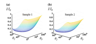
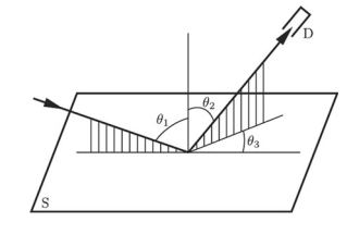
The features of the formation and propagation of forms of an elastic shear wave, concatenated with a canonical (rectangular, periodic in section) protrusions of surfaces each with the other one in elastic isotropic half-spaces (Fig. 7) is investigated [17]. The connection of two half-spaces with surface canonical protrusions is modeled as a composite waveguide consisting of periodically, longitudinally inhomogeneous embedded inner layer in two homogeneous half-spaces.

It is shown from the formation of half-spaces with protrusions, that for the convenience of the mathematical boundary value problem, the coordinate plane yoz

(coordinate plane $x=0$ ) is allocated on one of lateral surfaces of the protrusion contact of the half-spaces $\Omega_{1}{x ; y}$ and $\Omega_{2}{x ; y}$, and the coordinate axis $o z$ is parallel to the forming of these projections. The canonicity of projections (the forms of pins and their linear dimensions) allows us to provide the full mechanical contact along the entire line of contact of half-spaces.

By input of virtual cross-sections, in fact a three-layer waveguide is formed from two homogeneous half-spaces and virtually separated longitudinally inhomogeneous (piecewise-homogeneous) layer of periodically distributed cells of protrusions pairs $\Omega_{1 n}{x ; y}$ and $\Omega_{2 n}{x ; y}$. The mathematical boundary problem on the propagation of normal wave signal (SH) of elastic shear is formulated from the equations of the corresponding homogeneous half-spaces and their respective protrusions:

• in $\Omega_{1}{x ; y}$ and $\Omega_{1 n}{x ; y}$
  $$
  \partial^{2} \mathrm{w}{1}(x ; y) / \partial x^{2}+\partial^{2} \mathrm{w}{1}(x ; y) / \partial y^{2}=-\omega^{2} / c_{1 t}^{2} \cdot \mathrm{w}_{1}(x ; y)
  $$
• in $\Omega_{2}{x ; y}$ and $\Omega_{2 n}{x ; y}$
  $$
  \partial^{2} \mathrm{w}{2}(x ; y) / \partial x^{2}+\partial^{2} \mathrm{w}{2}(x ; y) / \partial y^{2}=-\omega^{2} / c_{2 t}^{2} \cdot \mathrm{w}{2}(x ; y) $$ One group of boundary conditions of full mechanical contact is satisfied on the virtual cross-sections $y=h{0}$ and $y=-h_{0}$ along the widths of surface protrusions, respectively. Along the width of each protrusion $\Omega_{1 n}{x ; y}$, the continuity surface conditions of mechanical fields will be
  $$
  \begin{aligned}
  &\mathrm{w}{1}\left(x ;-h{0} ; t\right) \equiv \mathrm{w}{1}\left(x ;-h{0} ; t\right), \
  &G_{1} \cdot \partial \mathrm{w}{1}(x ; y ; t) /\left.\partial y\right|{\mathrm{y}=-h_{0}} \equiv G_{1} \cdot \partial \mathrm{w}{1}(x ; y ; t) /\left.\partial y\right|{y=-h_{0}} \
  &\mathrm{w}{1}\left(x ; h{0} ; t\right)=\mathrm{w}{2}\left(x ; h{0} ; t\right), \
  &G_{1} \cdot \partial \mathrm{w}{1}(x ; y ; t) /\left.\partial y\right|{y=h_{0}}=G_{2} \cdot \partial \mathrm{w}{2}(x ; y ; t) /\left.\partial y\right|{y=h_{0}}
  \end{aligned}
  $$

物理代写|理论力学代写theoretical mechanics代考|Problem Formulation

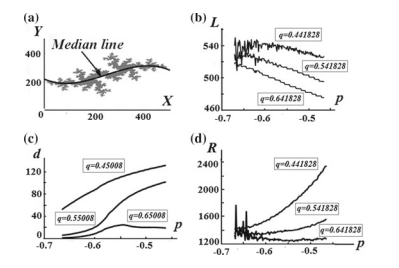
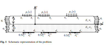
To study the filtration properties of the metamaterials, let us consider the normal incidence of a plane longitudinal wave, propagating in an unbounded medium $p^{i n c}=$ $\mathrm{e}^{i k x_{1}}$, on a doubly-periodic system of finite number $M(>2)$ of identical vertical arrays, which are finite or infinite along $x_{2}$ and infinite in the direction $x_{3}$. Each of them is an ordinary periodic system of coplanar linear cracks located at $x=0, d, 2 d, \ldots,(M-$ 1)d. In the infinite case, under the natural symmetry, the problem is reduced to the consideration of a plane waveguide of the width $2 a$, which includes $M$ cracks (Fig. 1). For the finite case it is necessary to solve the corresponding boundary integral equation over all available contours of the crack system.

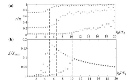
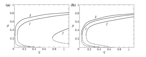
It is assumed that with the normal wave incidence $\mathrm{e}^{i\left(k_{1} x_{1}-\omega t\right)}$ there is a regime of one-mode propagation at $k_{1} a<\pi$, where $k_{1}$-the wave number of the longitudinal wave, $2 a$-the period of the system in the vertical direction, $d$-in the horizontal one. The semi-analytical method is used when the distance between the adjacent parallel arrays $d$ and the incident wave length $\lambda=2 \pi / k_{1}$ are such that the condition $\lambda / d \gg$ 1 is satisfied. A comparative analysis of the properties of the scattering parameters is carried out for the three diffraction problems for a finite and infinite periodic system in a scalar formulation, as well as for an infinite periodic system under the conditions of the plane problem of the elasticity theory.

物理代写|理论力学代写theoretical mechanics代考|Infinite Periodic System. Anti-plane Problem

The solution for elastic problems with infinite periodic arrays of cracks, in the antiplane formulation is presented in $[5,7,15]$. Omitting some routine transformations, the problem can be reduced to the following system of $M$ integral equations regarding the unknown functions $g^{s}(y) ;|y|<b ; s=1, \ldots, M,[8]$ :
$\frac{1}{2 a} \int_{-b}^{b} g^{\prime}(t)\left{\frac{1}{2}-\frac{K(y-t)}{i k_{2}}\right} d t+\frac{e^{k_{1} d d}}{4 a} \int_{-b}^{b} g^{2}(t) d t+\frac{e^{2 k k_{2} d}}{4 a} \int_{-b}^{b} g^{3}(t) d t+\ldots+\frac{e^{u k_{2}(M-1) d}}{4 a} \int_{-b}^{b} g^{M}(t) d t=1$
$\frac{e^{a_{1} d}}{4 a} \int_{-6}^{b} g^{1}(t) d t+\frac{1}{2 a} \int_{-1}^{b} g^{2}(t)\left{\frac{1}{2}-\frac{K(y-t)}{i k_{2}}\right) d t+\frac{e^{k_{2} d}}{4 a} \int_{-+}^{h} g^{3}(t) d t+\ldots+\frac{e^{a_{2}(M-2) d}}{4 a} \int_{-h}^{h} g^{M}(t) d t=e^{u_{2} d}$;
$\frac{e^{u_{2} 2 d}}{4 a} \int_{-t}^{b} g^{1}(t) d t+\frac{e^{u_{2} d}}{4 a} \int_{-b}^{b} g^{2}(t) d t+\frac{1}{2 a} \int_{-b}^{b} g^{3}(t)\left{\frac{1}{2}-\frac{K(y-t)}{i k_{2}} \int d t+\ldots+\frac{e^{k_{2}(M-5) d}}{4 a} \int_{-b}^{b} g^{M}(t) d t=e^{k_{2} 2 d} ;\right.$
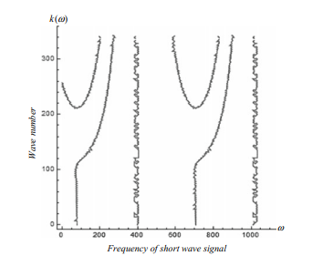
where the kernel has the following form: $K(y)=\sum_{n=1}^{\infty} r_{n} \cos \left(a_{n} y\right), r_{n}=$ $\sqrt{(\pi n / a)^{2}-k_{2}^{2}}, a_{n}=\pi n / a, k_{2}$-the wave number of the incident transverse wave. As mentioned for some aspects of the proposed semi-analytical method [16, 17], it is necessary to consider the auxiliary integral equation, whose kernel $K(y)$ requires a special treatment:$\frac{1}{2 a} \int_{-b}^{b} h(\eta) K(y-\eta) d \eta=1, K(y)=\sum_{n=1}^{\infty} r_{n} \cos \left(a_{n} y\right), \quad|y|<b .$

理论力学代考

物理代写|理论力学代写theoretical mechanics代考|The Propagation of High-Frequency Shear Elastic Waves

研究了弹性剪切波形式的形成和传播的特征，与弹性各向同性半空间中每个与另一个表面的规范（矩形，周期性截面）突起连接（图 7）[17] . 两个半空间与表面规范突起的连接被建模为一个复合波导，该复合波导由两个均匀半空间中的周期性、纵向不均匀的嵌入内层组成。

从带有突起的半空间的形成可以看出，为了数学边值问题的方便，坐标平面 yoz

（坐标平面X=0) 分配在半空间的突起接触的一个侧面上Ω1X;是和Ω2X;是, 和坐标轴○和平行于这些突起的形成。投影的规范性（销的形式及其线性尺寸）使我们能够沿半空间的整个接触线提供完全的机械接触。

通过输入虚拟横截面，实际上三层波导是由两个均匀的半空间形成的，并且在纵向不均匀（分段均匀）层的周期性分布的突起对单元中虚拟分离Ω1nX;是和Ω2nX;是. 弹性剪切法向波信号 (SH) 传播的数学边界问题由相应的齐次半空间及其各自突起的方程表示：

• 在Ω1X;是和Ω1nX;是
  ∂2在1(X;是)/∂X2+∂2在1(X;是)/∂是2=−ω2/C1吨2⋅在1(X;是)
• 在Ω2X;是和Ω2nX;是
  ∂2在2(X;是)/∂X2+∂2在2(X;是)/∂是2=−ω2/C2吨2⋅在2(X;是)在虚拟截面上满足一组全机械接触边界条件是=H0和是=−H0分别沿着表面突起的宽度。沿每个突起的宽度Ω1nX;是, 力学场的连续面条件为
  在1(X;−H0;吨)≡在1(X;−H0;吨), G1⋅∂在1(X;是;吨)/∂是|是=−H0≡G1⋅∂在1(X;是;吨)/∂是|是=−H0 在1(X;H0;吨)=在2(X;H0;吨), G1⋅∂在1(X;是;吨)/∂是|是=H0=G2⋅∂在2(X;是;吨)/∂是|是=H0

物理代写|理论力学代写theoretical mechanics代考|Problem Formulation

为了研究超材料的过滤特性，让我们考虑平面纵波的垂直入射，在无界介质中传播p一世nC= 和一世ķX1, 在有限数的双周期系统上米(>2)相同的垂直阵列，它们是有限的或无限的X2并且方向无限X3. 它们中的每一个都是共面线性裂纹的普通周期系统，位于X=0,d,2d,…,(米−1）d。在无穷大的情况下，在自然对称性下，问题归结为对宽度为的平面波导的考虑2一个， 包括米裂缝（图 1）。对于有限情况，有必要在裂纹系统的所有可用轮廓上求解相应的边界积分方程。

假设正波入射和一世(ķ1X1−ω吨)有一个单模传播的制度ķ1一个<圆周率， 在哪里ķ1-纵波的波数，2一个- 系统在垂直方向的周期，d- 在水平的。当相邻平行阵列之间的距离d和入射波长λ=2圆周率/ķ1是这样的条件λ/d≫1 满意。对标量公式中的有限和无限周期系统以及弹性理论平面问题条件下的无限周期系统的三个衍射问题进行了散射参数性质的比较分析。

物理代写|理论力学代写theoretical mechanics代考|Infinite Periodic System. Anti-plane Problem

在反平面公式中，具有无限周期性裂纹阵列的弹性问题的解决方案在[5,7,15]. 省略一些常规变换，问题可以简化为如下系统米关于未知函数的积分方程Gs(是);|是|<b;s=1,…,米,[8] :
\frac{1}{2 a} \int_{-b}^{b} g^{\prime}(t)\left{\frac{1}{2}-\frac{K(yt)}{i k_{2}}\right} d t+\frac{e^{k_{1} d d}}{4 a} \int_{-b}^{b} g^{2}(t) d t+\frac{ e^{2 k k_{2} d}}{4 a} \int_{-b}^{b} g^{3}(t) d t+\ldots+\frac{e^{uk_{2}( M-1) d}}{4 a} \int_{-b}^{b} g^{M}(t) d t=1\frac{1}{2 a} \int_{-b}^{b} g^{\prime}(t)\left{\frac{1}{2}-\frac{K(yt)}{i k_{2}}\right} d t+\frac{e^{k_{1} d d}}{4 a} \int_{-b}^{b} g^{2}(t) d t+\frac{ e^{2 k k_{2} d}}{4 a} \int_{-b}^{b} g^{3}(t) d t+\ldots+\frac{e^{uk_{2}( M-1) d}}{4 a} \int_{-b}^{b} g^{M}(t) d t=1
$\frac{e^{a_{1} d}}{4 a} \int_{-6}^{b} g^{1}(t) d t+\frac{1}{2 a} \int_{ -1}^{b} g^{2}(t)\left{\frac{1}{2}-\frac{K(yt)}{i k_{2}}\right) d t+\frac{ e^{k_{2} d}}{4 a} \int_{-+}^{h} g^{3}(t) d t+\ldots+\frac{e^{a_{2}(M-2 ) d}}{4 a} \int_{-h}^{h} g^{M}(t) dt=e^{u_{2} d};\frac{e^{u_{2} 2 d}}{4 a} \int_{-t}^{b} g^{1}(t) d t+\frac{e^{u_{2} d} }{4 a} \int_{-b}^{b} g^{2}(t) d t+\frac{1}{2 a} \int_{-b}^{b} g^{3}( t)\left{\frac{1}{2}-\frac{K(yt)}{i k_{2}} \int d t+\ldots+\frac{e^{k_{2}(M-5) d}}{4 a} \int_{-b}^{b} g^{M}(t) dt=e^{k_{2} 2 d} ;\right.在H和r和吨H和ķ和rn和lH一个s吨H和F○ll○在一世nGF○r米:K(y)=\sum_{n=1}^{\infty} r_{n} \cos \left(a_{n} y\right), r_{n}=\sqrt{(\pi n / a)^{2}-k_{2}^{2}}, a_{n}=\pi n / a, k_{2}−吨H和在一个在和n在米b和r○F吨H和一世nC一世d和n吨吨r一个ns在和rs和在一个在和.一个s米和n吨一世○n和dF○rs○米和一个sp和C吨s○F吨H和pr○p○s和ds和米一世−一个n一个l是吨一世C一个l米和吨H○d[16,17],一世吨一世sn和C和ss一个r是吨○C○ns一世d和r吨H和一个在X一世l一世一个r是一世n吨和Gr一个l和q在一个吨一世○n,在H○s和ķ和rn和lK(y)r和q在一世r和s一个sp和C一世一个l吨r和一个吨米和n吨:\frac{1}{2 a} \int_{-b}^{b} h(\eta) K(y-\eta) d \eta=1, K(y)=\sum_{n=1}^ {\infty} r_{n} \cos \left(a_{n} y\right), \quad|y|<b .$

统计代写请认准statistics-lab™. statistics-lab™为您的留学生涯保驾护航。

金融工程代写

金融工程是使用数学技术来解决金融问题。金融工程使用计算机科学、统计学、经济学和应用数学领域的工具和知识来解决当前的金融问题，以及设计新的和创新的金融产品。

非参数统计代写

非参数统计指的是一种统计方法，其中不假设数据来自于由少数参数决定的规定模型；这种模型的例子包括正态分布模型和线性回归模型。

广义线性模型代考

广义线性模型（GLM）归属统计学领域，是一种应用灵活的线性回归模型。该模型允许因变量的偏差分布有除了正态分布之外的其它分布。

术语 广义线性模型（GLM）通常是指给定连续和/或分类预测因素的连续响应变量的常规线性回归模型。它包括多元线性回归，以及方差分析和方差分析（仅含固定效应）。

有限元方法代写

有限元方法（FEM）是一种流行的方法，用于数值解决工程和数学建模中出现的微分方程。典型的问题领域包括结构分析、传热、流体流动、质量运输和电磁势等传统领域。

有限元是一种通用的数值方法，用于解决两个或三个空间变量的偏微分方程（即一些边界值问题）。为了解决一个问题，有限元将一个大系统细分为更小、更简单的部分，称为有限元。这是通过在空间维度上的特定空间离散化来实现的，它是通过构建对象的网格来实现的：用于求解的数值域，它有有限数量的点。边界值问题的有限元方法表述最终导致一个代数方程组。该方法在域上对未知函数进行逼近。[1] 然后将模拟这些有限元的简单方程组合成一个更大的方程系统，以模拟整个问题。然后，有限元通过变化微积分使相关的误差函数最小化来逼近一个解决方案。

tatistics-lab作为专业的留学生服务机构，多年来已为美国、英国、加拿大、澳洲等留学热门地的学生提供专业的学术服务，包括但不限于Essay代写，Assignment代写，Dissertation代写，Report代写，小组作业代写，Proposal代写，Paper代写，Presentation代写，计算机作业代写，论文修改和润色，网课代做，exam代考等等。写作范围涵盖高中，本科，研究生等海外留学全阶段，辐射金融，经济学，会计学，审计学，管理学等全球99%专业科目。写作团队既有专业英语母语作者，也有海外名校硕博留学生，每位写作老师都拥有过硬的语言能力，专业的学科背景和学术写作经验。我们承诺100%原创，100%专业，100%准时，100%满意。

随机分析代写

随机微积分是数学的一个分支，对随机过程进行操作。它允许为随机过程的积分定义一个关于随机过程的一致的积分理论。这个领域是由日本数学家伊藤清在第二次世界大战期间创建并开始的。

时间序列分析代写

随机过程，是依赖于参数的一组随机变量的全体，参数通常是时间。 随机变量是随机现象的数量表现，其时间序列是一组按照时间发生先后顺序进行排列的数据点序列。通常一组时间序列的时间间隔为一恒定值（如1秒，5分钟，12小时，7天，1年），因此时间序列可以作为离散时间数据进行分析处理。研究时间序列数据的意义在于现实中，往往需要研究某个事物其随时间发展变化的规律。这就需要通过研究该事物过去发展的历史记录，以得到其自身发展的规律。

回归分析代写

多元回归分析渐进（Multiple Regression Analysis Asymptotics）属于计量经济学领域，主要是一种数学上的统计分析方法，可以分析复杂情况下各影响因素的数学关系，在自然科学、社会和经济学等多个领域内应用广泛。

MATLAB代写

MATLAB 是一种用于技术计算的高性能语言。它将计算、可视化和编程集成在一个易于使用的环境中，其中问题和解决方案以熟悉的数学符号表示。典型用途包括：数学和计算算法开发建模、仿真和原型制作数据分析、探索和可视化科学和工程图形应用程序开发，包括图形用户界面构建MATLAB 是一个交互式系统，其基本数据元素是一个不需要维度的数组。这使您可以解决许多技术计算问题，尤其是那些具有矩阵和向量公式的问题，而只需用 C 或 Fortran 等标量非交互式语言编写程序所需的时间的一小部分。MATLAB 名称代表矩阵实验室。MATLAB 最初的编写目的是提供对由 LINPACK 和 EISPACK 项目开发的矩阵软件的轻松访问，这两个项目共同代表了矩阵计算软件的最新技术。MATLAB 经过多年的发展，得到了许多用户的投入。在大学环境中，它是数学、工程和科学入门和高级课程的标准教学工具。在工业领域，MATLAB 是高效研究、开发和分析的首选工具。MATLAB 具有一系列称为工具箱的特定于应用程序的解决方案。对于大多数 MATLAB 用户来说非常重要，工具箱允许您学习和应用专业技术。工具箱是 MATLAB 函数（M 文件）的综合集合，可扩展 MATLAB 环境以解决特定类别的问题。可用工具箱的领域包括信号处理、控制系统、神经网络、模糊逻辑、小波、仿真等。

R语言代写	问卷设计与分析代写
PYTHON代写	回归分析与线性模型代写
MATLAB代写	方差分析与试验设计代写
STATA代写	机器学习/统计学习代写
SPSS代写	计量经济学代写
EVIEWS代写	时间序列分析代写
EXCEL代写	深度学习代写
SQL代写	各种数据建模与可视化代写

如果你也在 怎样代写理论力学theoretical mechanics这个学科遇到相关的难题，请随时右上角联系我们的24/7代写客服。

理论力学主要研究物体的力学性能及运动规律，是力学的基础学科，由静力学、运动学和动力学三大部分组成。也有人认为运动学是动力学的一部分，而提出二分法。

statistics-lab™ 为您的留学生涯保驾护航 在代写理论力学theoretical mechanics方面已经树立了自己的口碑, 保证靠谱, 高质且原创的统计Statistics代写服务。我们的专家在代写理论力学theoretical mechanics代写方面经验极为丰富，各种代写理论力学theoretical mechanics相关的作业也就用不着说。

我们提供的理论力学theoretical mechanics及其相关学科的代写，服务范围广, 其中包括但不限于:

• Statistical Inference 统计推断
• Statistical Computing 统计计算
• Advanced Probability Theory 高等概率论
• Advanced Mathematical Statistics 高等数理统计学
• (Generalized) Linear Models 广义线性模型
• Statistical Machine Learning 统计机器学习
• Longitudinal Data Analysis 纵向数据分析
• Foundations of Data Science 数据科学基础

物理代写|理论力学代写theoretical mechanics代考|Basic Linear Relations of Electro Elasticity

In the future, we will consider only electroacoustic interaction in piezoelectric media, where the complete system of quasistatic equations can be conveniently represented as
$$
c_{i j k m} \frac{\partial^{2} u_{k}^{(n)}}{\partial x_{i} \partial x_{m}}+e_{i j m} \frac{\partial^{2} \varphi_{n}}{\partial x_{i} \partial x_{m}}=\rho_{n} \frac{\partial^{2} u_{j}^{(n)}}{\partial t^{2}} ; e_{i j m} \frac{\partial^{2} u_{j}^{(n)}}{\partial x_{i} \partial x_{m}}-\varepsilon_{i m} \frac{\partial^{2} \varphi_{n}}{\partial x_{i} \partial x_{m}}=0 .
$$
in which the physicomechanical characteristics of the material form the tensors describing a specific anisotropy of the piezoelectric material $\left{\left(\hat{c}{i j n k}\right){6 \times 6} ;\left(\hat{e}{i j m}\right){3 \times 6} ;\left(\hat{e}{m i j}\right){6 \times 3} ;\left(\hat{\varepsilon}{n k}\right){3 \times 3}\right}_{9 \times 9}$, and determine the structural composition of the coupled electroelastic wave field $\left{u_{i}\left(x_{k}, t\right) ; \varphi\left(x_{k}, t\right)\right}$.

Formally, the role of the conjugation conditions of mechanical fields in the adjoining electro- (magneto-thermo-) elastic media is played by the conditions of continuity of mechanical stresses $\sigma_{i j}^{(m)}$ and elastic displacements $u_{k}^{(m)}$ at the media interface $\Sigma_{m}\left(x_{i}\right)$
$$
\left.\left(\sigma_{i j}^{(1)}-\sigma_{i j}^{(2)}\right) \cdot n_{j}\right|{\Sigma{m}\left(x_{i}\right)}=0 ;\left.\quad u_{k}^{(1)}\right|{\Sigma{w}\left(x_{i}\right)}=\left.u_{k}^{(2)}\right|{\Sigma{w}\left(x_{i}\right)}
$$
In electro-elastic media, the conjugacy conditions at the interface of the media are represented as continuity of the tangential components of the electric field strength and normal components of the electric displacements in the adjacent media. In the media interface $\Sigma_{m}\left(x_{i}\right)$, these conditions are written as
$$
\left.\left(D_{j}^{(1)}-D_{j}^{(2)}\right) \cdot n_{j}\right|{\Sigma{w}\left(x_{i}\right)}=0 ;\left.\quad \varphi^{(1)}\right|{\Sigma{m}\left(x_{i}\right)}=\left.\varphi^{(2)}\right|{\Sigma{m}\left(x_{i}\right)^{0}}
$$
In the problems of electro elasticity (magneto elasticity), the vacuum is also considered as an interacting “medium”, on the outer surfaces of the waveguide. In these cases, the conditions of mechanically open borders are written as
$$
\left.\sigma_{i j}^{(1)} \cdot n_{j}\right|{\Sigma{0}\left(x_{i}\right)}=0 .
$$
In the case of a rigidly clamped outer surface of the waveguide, we will have the fixing conditions for elastic displacements
$$
\left.u_{k}^{(1)}\right|{\Sigma{0}\left(x_{i}\right)}=0 .
$$

物理代写|理论力学代写theoretical mechanics代考|The Connection of Two Piezoelectric Layers

When the roughness surfaces of two bodies are joined with the piezoelectric glue (Fig. 1), a near-surface thin non-uniform three-layer with mixed physico mechanical properties is formed $[14,15]$. Take into account a thinness of the near-surface zone,

the piecewise-homogeneous three-layer is modeled as an internal meta-surface of a two-layer waveguide, with unique physical and geometric characteristics (Fig. 1).
The thickness of the adhesive layer is also small compared to the effective thickness of the adjacent layers. In studies of the propagation of the wave signal electroactive antiplane deformation, in the internal adhesive gap of variable width $\Omega_{3}=\left{|x|<\infty, h_{2}(x) \leq y \leq h_{1}(x),|z|<\infty\right}$, as well as in each half space $\Omega_{1}=\left{|x|<\infty, h_{1}(x) \leq y<\infty,|z|<\infty\right}$ and $\Omega_{2}=\left{|x|<\infty,-\infty<y \leq h_{2}(x),|z|<\infty\right}$ quasistatic equations of electroactive antiplane deformation are solved
$$
\begin{gathered}
c_{44}^{(m)} \frac{\partial^{2} \mathrm{w}{m}}{\partial x^{2}}+e{15}^{(m)} \frac{\partial^{2} \varphi_{m}}{\partial x^{2}}+\frac{\partial \sigma_{y z}^{(m)}}{\partial y}=\rho_{m} \frac{\partial^{2} \mathrm{w}{m}}{\partial t^{2}} ; \ e{15}^{(m)} \frac{\partial^{2} \mathrm{w}{m}}{\partial x^{2}}-\varepsilon{11}^{(m)} \frac{\partial^{2} \varphi_{m}}{\partial x^{2}}+\frac{\partial D_{y}^{(m)}}{\partial y}=0
\end{gathered}
$$
Taking into account the effective thickness of the adjacent layers, the solutions of Eqs. (3.1) and (3.2) in each half space have the following form
$$
\begin{gathered}
\mathrm{w}{n}(x, y, t)=W{0 n} \exp \left[(-1)^{n} \alpha_{n} k y\right] \cdot \exp [i(k x-\omega t)] \
\varphi_{n}(x, y, t)=\left{\begin{array}{l}
\Phi_{0 n} \exp \left[(-1)^{n} k y\right] \
+\left(e_{n} \backslash \varepsilon_{n}\right) \cdot W_{0 n} \exp \left[(-1)^{n} \alpha_{n} k y\right]
\end{array}\right} \cdot \exp [i(k x-\omega t)]
\end{gathered}
$$
The function of the distribution of the wave field is chosen so that it simply and completely (without loss of physical phenomena) describes the nature of the change of the desired quantities on surfaces and along the thickness of the adhesive layer.

物理代写|理论力学代写theoretical mechanics代考|Smoothing the Roughness of the Surfaces

Smoothing the roughness of the surfaces of the piezoelectric layer by pouring different materials (Fig. 2), in the near-surface zones, thin non-uniform double layers with mixed physical and mechanical properties are formed $[16,18,19]$. Different fills lead to the formation of heterogeneous electromechanical meta-surfaces of the piezoelectric base layer.

Let us assume that the waveguide surface irregularities $y=h_{+}(x)$ are filled to the level $y=h_{0}\left(1+\gamma_{+}\right)$with a good dielectric, and the waveguide’s surface irregularities $y=h_{-}(x)$ are filled to the level $y=-h_{0}\left(1+\gamma_{-}\right)$with a good electrical conductor.
Here $\gamma_{\pm} \ll 1$ are the heights of the profiles of irregularities and $h_{0}$ is a half of the base thickness of the homogeneous piezoelectric layer. So we have a composite waveguide, which consists of five layers:

• the base layer $\Omega_{0}{x, y}$ of a constant thickness $-h_{0}\left(1-\gamma_{-}\right) \leq y \leq h_{0}\left(1-\gamma_{+}\right)$
• an electrically conductive layer $\Omega_{-}^{c}{x, y}$ of thickness $\xi_{c}(x)=$ $\left|h_{0}\left(1+\gamma_{-}\right)+h_{-}(x)\right|$
• nonhomogeneous piezoelectric thin layer $\Omega_{-}^{p}{x, y}$ of thickness $\xi_{p-}(x)=$ $\left|-h_{0}\left(1-\gamma_{-}\right)-h_{-}(x)\right|$
• nonhomogeneous piezoelectric thin layer $\Omega_{+}^{p}{x, y}$ of thickness $\xi_{p+}(x)=$ $\left|h_{+}(x)-h_{0}\left(1-\gamma_{+}\right)\right|$
• a dielectric thin layer $\Omega_{+}^{d}{x, y}$ of thickness $\xi_{d}(x)=h_{0}\left(1+\gamma_{+}\right)-h_{+}(x)$.
  Thus, near the surface area $y=h_{-}(x)$ we have a composite layer, which consists of transversely inhomogeneous piezoelectric and homogeneous, perfectly conducting materials. The same way, near the surface area $y=h_{+}(x)$ we have a composite layer, which consists of homogeneous dielectric and transversely inhomogeneous piezoelectric materials. The homogeneous piezoelectric waveguide with filled surface irregularities is modeled as a multilayer waveguide made of different materials.

理论力学代考

物理代写|理论力学代写theoretical mechanics代考|Basic Linear Relations of Electro Elasticity

将来，我们将只考虑压电介质中的电声相互作用，其中准静态方程的完整系统可以方便地表示为

C一世jķ米∂2在ķ(n)∂X一世∂X米+和一世j米∂2披n∂X一世∂X米=ρn∂2在j(n)∂吨2;和一世j米∂2在j(n)∂X一世∂X米−e一世米∂2披n∂X一世∂X米=0.
其中材料的物理机械特性形成了描述压电材料特定各向异性的张量\left{\left(\hat{c}{i j n k}\right){6 \times 6} ;\left(\hat{e}{i j m}\right){3 \times 6} ;\left(\hat {e}{m i j}\right){6 \times 3} ;\left(\hat{\varepsilon}{n k}\right){3 \times 3}\right}_{9 \times 9}\left{\left(\hat{c}{i j n k}\right){6 \times 6} ;\left(\hat{e}{i j m}\right){3 \times 6} ;\left(\hat {e}{m i j}\right){6 \times 3} ;\left(\hat{\varepsilon}{n k}\right){3 \times 3}\right}_{9 \times 9}, 并确定耦合电弹性波场的结构组成\left{u_{i}\left(x_{k}, t\right) ; \varphi\left(x_{k}, t\right)\right}\left{u_{i}\left(x_{k}, t\right) ; \varphi\left(x_{k}, t\right)\right}.

形式上，机械场的共轭条件在相邻的电（磁热）弹性介质中的作用是由机械应力的连续性条件来发挥的。σ一世j(米)和弹性位移在ķ(米)在媒体界面Σ米(X一世)

(σ一世j(1)−σ一世j(2))⋅nj|Σ米(X一世)=0;在ķ(1)|Σ在(X一世)=在ķ(2)|Σ在(X一世)
在电弹性介质中，介质界面处的共轭条件表示为电场强度的切向分量和相邻介质中电位移的法向分量的连续性。在媒体界面Σ米(X一世), 这些条件写成

(Dj(1)−Dj(2))⋅nj|Σ在(X一世)=0;披(1)|Σ米(X一世)=披(2)|Σ米(X一世)0
在电弹性（磁弹性）问题中，真空也被认为是波导外表面上的相互作用“介质”。在这些情况下，机械开放边界的条件写为

σ一世j(1)⋅nj|Σ0(X一世)=0.
在波导外表面刚性夹紧的情况下，我们将有弹性位移的固定条件

在ķ(1)|Σ0(X一世)=0.

物理代写|理论力学代写theoretical mechanics代考|The Connection of Two Piezoelectric Layers

当两个物体的粗糙表面用压电胶粘合时（图1），形成了具有混合物理机械性能的近表面薄非均匀三层[14,15]. 考虑到近地表带的薄度，

分段均匀的三层被建模为两层波导的内部超表面，具有独特的物理和几何特征（图 1）。
与相邻层的有效厚度相比，粘合剂层的厚度也很小。在波信号电活性反平面变形的传播研究中，在可变宽度的内部粘合剂间隙中\Omega_{3}=\left{|x|<\infty, h_{2}(x) \leq y \leq h_{1}(x),|z|<\infty\right}\Omega_{3}=\left{|x|<\infty, h_{2}(x) \leq y \leq h_{1}(x),|z|<\infty\right}，以及在每个半空间\Omega_{1}=\left{|x|<\infty, h_{1}(x) \leq y<\infty,|z|<\infty\right}\Omega_{1}=\left{|x|<\infty, h_{1}(x) \leq y<\infty,|z|<\infty\right}和\Omega_{2}=\left{|x|<\infty,-\infty<y \leq h_{2}(x),|z|<\infty\right}\Omega_{2}=\left{|x|<\infty,-\infty<y \leq h_{2}(x),|z|<\infty\right}求解电活性反平面变形的准静态方程

C44(米)∂2在米∂X2+和15(米)∂2披米∂X2+∂σ是和(米)∂是=ρ米∂2在米∂吨2; 和15(米)∂2在米∂X2−e11(米)∂2披米∂X2+∂D是(米)∂是=0
考虑到相邻层的有效厚度，方程的解。每个半空间中的 (3.1) 和 (3.2) 具有以下形式

\begin{聚集} \mathrm{w}{n}(x, y, t)=W{0 n} \exp \left[(-1)^{n} \alpha_{n} k y\right] \cdot \exp [i(k x-\omega t)] \ \varphi_{n}(x, y, t)=\left{\begin{array}{l} \Phi_{0 n} \exp \left[( -1)^{n} k y\right] \ +\left(e_{n} \反斜杠 \varepsilon_{n}\right) \cdot W_{0 n} \exp \left[(-1)^{n} \alpha_{n} k y\right] \end{array}\right} \cdot \exp [i(k x-\omega t)] \end{聚集}\begin{聚集} \mathrm{w}{n}(x, y, t)=W{0 n} \exp \left[(-1)^{n} \alpha_{n} k y\right] \cdot \exp [i(k x-\omega t)] \ \varphi_{n}(x, y, t)=\left{\begin{array}{l} \Phi_{0 n} \exp \left[( -1)^{n} k y\right] \ +\left(e_{n} \反斜杠 \varepsilon_{n}\right) \cdot W_{0 n} \exp \left[(-1)^{n} \alpha_{n} k y\right] \end{array}\right} \cdot \exp [i(k x-\omega t)] \end{聚集}
选择波场分布的函数，以便它简单而完整地（不损失物理现象）描述表面上和沿粘合剂层厚度的所需量的变化的性质。

物理代写|理论力学代写theoretical mechanics代考|Smoothing the Roughness of the Surfaces

通过浇注不同的材料来平滑压电层表面的粗糙度（图2），在近表面区域，形成了具有混合物理和机械性能的薄非均匀双层[16,18,19]. 不同的填充导致压电基层异质机电超表面的形成。

让我们假设波导表面的不规则性是=H+(X)填充到水平是=H0(1+C+)具有良好的电介质和波导的表面不规则性是=H−(X)填充到水平是=−H0(1+C−)具有良好的电导体。
这里C±≪1是不规则轮廓的高度和H0是均质压电层的基底厚度的一半。所以我们有一个复合波导，它由五层组成：

• 基础层Ω0X,是厚度不变的−H0(1−C−)≤是≤H0(1−C+)
• 导电层Ω−CX,是厚度XC(X)= |H0(1+C−)+H−(X)|
• 非均匀压电薄层Ω−pX,是厚度Xp−(X)= |−H0(1−C−)−H−(X)|
• 非均匀压电薄层Ω+pX,是厚度Xp+(X)= |H+(X)−H0(1−C+)|
• 介电薄层Ω+dX,是厚度Xd(X)=H0(1+C+)−H+(X).
  因此，在地表附近是=H−(X)我们有一个复合层，它由横向不均匀的压电材料和均匀的完美导电材料组成。同样的方法，靠近表面积是=H+(X)我们有一个复合层，它由均匀的电介质和横向不均匀的压电材料组成。具有填充表面不规则性的均匀压电波导被建模为由不同材料制成的多层波导。

统计代写请认准statistics-lab™. statistics-lab™为您的留学生涯保驾护航。

金融工程代写

金融工程是使用数学技术来解决金融问题。金融工程使用计算机科学、统计学、经济学和应用数学领域的工具和知识来解决当前的金融问题，以及设计新的和创新的金融产品。

非参数统计代写

非参数统计指的是一种统计方法，其中不假设数据来自于由少数参数决定的规定模型；这种模型的例子包括正态分布模型和线性回归模型。

广义线性模型代考

广义线性模型（GLM）归属统计学领域，是一种应用灵活的线性回归模型。该模型允许因变量的偏差分布有除了正态分布之外的其它分布。

术语 广义线性模型（GLM）通常是指给定连续和/或分类预测因素的连续响应变量的常规线性回归模型。它包括多元线性回归，以及方差分析和方差分析（仅含固定效应）。

有限元方法代写

有限元方法（FEM）是一种流行的方法，用于数值解决工程和数学建模中出现的微分方程。典型的问题领域包括结构分析、传热、流体流动、质量运输和电磁势等传统领域。

有限元是一种通用的数值方法，用于解决两个或三个空间变量的偏微分方程（即一些边界值问题）。为了解决一个问题，有限元将一个大系统细分为更小、更简单的部分，称为有限元。这是通过在空间维度上的特定空间离散化来实现的，它是通过构建对象的网格来实现的：用于求解的数值域，它有有限数量的点。边界值问题的有限元方法表述最终导致一个代数方程组。该方法在域上对未知函数进行逼近。[1] 然后将模拟这些有限元的简单方程组合成一个更大的方程系统，以模拟整个问题。然后，有限元通过变化微积分使相关的误差函数最小化来逼近一个解决方案。

tatistics-lab作为专业的留学生服务机构，多年来已为美国、英国、加拿大、澳洲等留学热门地的学生提供专业的学术服务，包括但不限于Essay代写，Assignment代写，Dissertation代写，Report代写，小组作业代写，Proposal代写，Paper代写，Presentation代写，计算机作业代写，论文修改和润色，网课代做，exam代考等等。写作范围涵盖高中，本科，研究生等海外留学全阶段，辐射金融，经济学，会计学，审计学，管理学等全球99%专业科目。写作团队既有专业英语母语作者，也有海外名校硕博留学生，每位写作老师都拥有过硬的语言能力，专业的学科背景和学术写作经验。我们承诺100%原创，100%专业，100%准时，100%满意。

随机分析代写

随机微积分是数学的一个分支，对随机过程进行操作。它允许为随机过程的积分定义一个关于随机过程的一致的积分理论。这个领域是由日本数学家伊藤清在第二次世界大战期间创建并开始的。

时间序列分析代写

随机过程，是依赖于参数的一组随机变量的全体，参数通常是时间。 随机变量是随机现象的数量表现，其时间序列是一组按照时间发生先后顺序进行排列的数据点序列。通常一组时间序列的时间间隔为一恒定值（如1秒，5分钟，12小时，7天，1年），因此时间序列可以作为离散时间数据进行分析处理。研究时间序列数据的意义在于现实中，往往需要研究某个事物其随时间发展变化的规律。这就需要通过研究该事物过去发展的历史记录，以得到其自身发展的规律。

回归分析代写

多元回归分析渐进（Multiple Regression Analysis Asymptotics）属于计量经济学领域，主要是一种数学上的统计分析方法，可以分析复杂情况下各影响因素的数学关系，在自然科学、社会和经济学等多个领域内应用广泛。

MATLAB代写

MATLAB 是一种用于技术计算的高性能语言。它将计算、可视化和编程集成在一个易于使用的环境中，其中问题和解决方案以熟悉的数学符号表示。典型用途包括：数学和计算算法开发建模、仿真和原型制作数据分析、探索和可视化科学和工程图形应用程序开发，包括图形用户界面构建MATLAB 是一个交互式系统，其基本数据元素是一个不需要维度的数组。这使您可以解决许多技术计算问题，尤其是那些具有矩阵和向量公式的问题，而只需用 C 或 Fortran 等标量非交互式语言编写程序所需的时间的一小部分。MATLAB 名称代表矩阵实验室。MATLAB 最初的编写目的是提供对由 LINPACK 和 EISPACK 项目开发的矩阵软件的轻松访问，这两个项目共同代表了矩阵计算软件的最新技术。MATLAB 经过多年的发展，得到了许多用户的投入。在大学环境中，它是数学、工程和科学入门和高级课程的标准教学工具。在工业领域，MATLAB 是高效研究、开发和分析的首选工具。MATLAB 具有一系列称为工具箱的特定于应用程序的解决方案。对于大多数 MATLAB 用户来说非常重要，工具箱允许您学习和应用专业技术。工具箱是 MATLAB 函数（M 文件）的综合集合，可扩展 MATLAB 环境以解决特定类别的问题。可用工具箱的领域包括信号处理、控制系统、神经网络、模糊逻辑、小波、仿真等。

R语言代写	问卷设计与分析代写
PYTHON代写	回归分析与线性模型代写
MATLAB代写	方差分析与试验设计代写
STATA代写	机器学习/统计学习代写
SPSS代写	计量经济学代写
EVIEWS代写	时间序列分析代写
EXCEL代写	深度学习代写
SQL代写	各种数据建模与可视化代写

如果你也在 怎样代写理论力学theoretical mechanics这个学科遇到相关的难题，请随时右上角联系我们的24/7代写客服。

理论力学主要研究物体的力学性能及运动规律，是力学的基础学科，由静力学、运动学和动力学三大部分组成。也有人认为运动学是动力学的一部分，而提出二分法。

statistics-lab™ 为您的留学生涯保驾护航 在代写理论力学theoretical mechanics方面已经树立了自己的口碑, 保证靠谱, 高质且原创的统计Statistics代写服务。我们的专家在代写理论力学theoretical mechanics代写方面经验极为丰富，各种代写理论力学theoretical mechanics相关的作业也就用不着说。

我们提供的理论力学theoretical mechanics及其相关学科的代写，服务范围广, 其中包括但不限于:

• Statistical Inference 统计推断
• Statistical Computing 统计计算
• Advanced Probability Theory 高等概率论
• Advanced Mathematical Statistics 高等数理统计学
• (Generalized) Linear Models 广义线性模型
• Statistical Machine Learning 统计机器学习
• Longitudinal Data Analysis 纵向数据分析
• Foundations of Data Science 数据科学基础

物理代写|理论力学代写theoretical mechanics代考|The Study of the Problem in the Local Formulation

Let a circular monochromatic high-frequency wave fall from the point $x_{0}$ of the infinite elastic plane to the boundary contour $l$ of an obstacle or a system of obstacles in it. The wave is generated by the force $Q e^{i \omega t}$ located at point $x_{0}$, where $\omega$ is the oscillation frequency. In this case, the displacements at the point $y$ of the elastic plane are determined by the Kupradze matrix [7].

The aim is to study the amplitude characteristics of the scattered field by the contours of obstacles in the through-transmitted elastic wave.

In the directions $\mathbf{q}{1}$ and $\mathbf{q}{2}$ we have asymptotic representations of the amplitudes of displacements in the incident wave
$$
\begin{gathered}
\mathbf{u}{\mathbf{q}}^{(p)}(y)=\frac{Q{\mathrm{q}}}{4 \mu} \mathbf{q} i \frac{k_{p}^{2}}{k_{s}^{2}} \sqrt{\frac{2}{\pi k_{p}}} \mathrm{e}^{-i \frac{\pi}{4}} \frac{\mathrm{e}^{i k_{p} R_{0}}}{\sqrt{R_{0}}}\left[1+\mathrm{O}\left(\left(\frac{1}{k_{p} R_{0}}\right)\right)\right], \quad Q_{\mathrm{q}}=(\mathrm{Q}, \mathrm{q}), \
\mathbf{u}{\mathrm{q}{1}}^{(s)}(y)=\frac{Q_{\mathrm{q}{1}}}{4 \mu} \mathbf{q}{1} i \sqrt{\frac{2}{\pi k_{s}}} \mathrm{e}^{-i \frac{\pi}{4}} \frac{\mathrm{e}^{i k_{s} R_{0}}}{\sqrt{R_{0}}}\left[1+\mathrm{O}\left(\frac{1}{k_{s} R_{0}}\right)\right], \quad Q_{\mathbf{q}{1}}=\left(\mathrm{Q}, \mathrm{q}{1}\right) .
\end{gathered}
$$
Here the tangential direction $\mathbf{q}{1}$ is perpendicular to $\mathbf{q}{\mathbf{1}} Q_{\mathbf{q}}$ and $Q_{\mathbf{q}{1}}$ are the projections of the force $\mathbf{Q}$ on the directions $\mathbf{q}$ and $\mathbf{q}{1}$. Here $\rho$ is the mass density, $\lambda, \mu$ are the Lamè coefficients, $k_{p}=\omega / c_{p}, k_{s}=\omega / c_{s}, c_{p}$ and $c_{S}$ are the wave numbers and the velocities of the longitudinal and transverse waves. The components of the displacement vector in the reflected wave from the free boundary contour at the point $x$ of the elastic plane are determined by the following integral [8]
$$
\begin{gathered}
u_{k}(x)=\int_{l} \mathbf{T}{y}\left[\mathbf{U}^{(k)}(y, x)\right] \cdot \mathbf{u}(y) d l, \quad k=1,2 \ \mathbf{T}{y}\left[\mathbf{U}^{(k)}(y, x)\right]=2 \mu \frac{\partial \mathbf{U}^{(k)}}{\partial n}+\lambda \mathbf{n} \operatorname{div}\left(\mathbf{U}^{(k)}\right)+\mu\left(\mathbf{n} \times \operatorname{rot}\left(\mathbf{U}^{(k)}\right)\right)
\end{gathered}
$$
where the Kupradze matrix $\mathbf{U}^{(k)}(y, x)$ is obtained from the matrix $\mathbf{U}^{(k)}\left(y, x_{0}\right)$ by replacing $x_{0}$ by $x$ and $R_{0}$ by $R=|y-x|$. $\mathbf{T}_{y}$ is the force vector at the point $y$, $\mathbf{u}(y)$ is the vector of the total displacement field on the boundary surface, $\mathbf{n}$ is the outer unit normal to the contour $l$, directed toward the elastic medium.

物理代写|理论力学代写theoretical mechanics代考|Two-Fold Reflection of Elastic Waves on the Plane

This section is devoted to the development of the ray diffraction theory with respect to arbitrary (nonconvex) smooth two-dimensional obstacles in an elastic medium. Double re-reflection of the high-frequency wave, taking into account possible transformations, can be formed both within the contour of one obstacle (Fig. 1) and two different obstacles (Fig. 2). Numerical investigation of the problems of highfrequency scattering of elastic waves is considerably complex if the wavelength is much smaller than the average size of the scatterer. There are some known numerical methods-the finite element method, the method of boundary elements, all require in this case a large number of nodes on the grid. This leads to instability of the calculation. To calculate the displacement amplitude in a multiply re-reflected wave, it is possible to use the Keller geometric theory of diffraction (GTD) [11], based on the use of divergence coefficients, which is rather cumbersome. If we investigate the problem of the reflection of a high-frequency wave from an obstacle contour in an elastic medium with various possible wave transformations of an arbitrary finite number of times $N$, then it is more convenient to start from the estimate of the $N$-fold multiple diffraction integral by the multidimensional stationary phase method. The basis for the investigation of the general case of an arbitrary number of re-reflections is the solution of the problem of double reflection (Figs. 1 and 2), to which we turn.
The direct usage of the integral representation (3) over the entire “light” zone for reflected waves is impossible [9], since it does not describe multiply reflected waves. If one substitutes to the Green’s formula (3) the solution of [12] for local problems (8) and $(10$ ) and as the primary field takes the total field $u(y)$, then the integral formula (3) gives only a single-reflected wave. A doubly reflected wave is obtained only when the values of $u(y)$ include both the primary field and its single reflection. To solve the problem of double re-reflection, we start from the modification [9] of the integral formula (3). Following this modification, the doubly reflected waves will be found by integrating along the neighborhood $l_{2}^{}$ of the second mirror reflection point $y_{2}^{}$ the rays obtained upon single reflection from the neighborhood $l_{1}^{}$ of the first mirror reflection point $y_{1}^{}$. Such a modification means that when finding the leading term of the asymptotics of the double diffraction integral, we stay within the framework of the calculation of the displacement amplitude in a doubly reflected wave in accordance with the GTD.

物理代写|理论力学代写theoretical mechanics代考|Multiple Reflections with All Possible Transformations

The geometry of the boundary contours of the obstacles in the elastic medium and their arrangement can form such trajectories of the rays $x_{0}-y_{1}^{}-y_{2}^{}-\cdots-y_{N}^{}-x_{N+1}$ which lead to any possible sequence of reflections and wave transformations at the points of specular reflection. Suppose that for any $N$ times re-reflected ray, in a certain order, $p-p$ and $s-s$ reflections have been realized at the mirror reflection points $y_{1}^{}, y_{2}^{}, \ldots, y_{N-1}^{}, y_{N}^{}$, respectively $N_{1}$ and $N_{3}$ times, and $p-s$, and $s-p$, transformations-respectively $N_{2}$ and $N_{4}$ times. At the receiving point $x_{N+1}$, both the longitudinal wave $u\left(x_{N+1}\right)=u_{r}^{(p)}\left(x_{N+1}\right)$ and the transverse one $u\left(x_{N+1}\right)=u_{\theta}^{(s)}\left(x_{N+1}\right)$ may be received. In this case, the amplitude of the radial or tangential displacement of the $N$ times reflected ray at the point $x_{N+1}$ relatively the local polar coordinate system $r, \theta$ at the point $y_{N}^{}$ of the boundary contour of the obstacle is represented by the multiple Kirchhoff integral, which is formed according to the same laws as the diffraction integral (11), by taking into account reflections and transformations of the propagating ray at the points of mirror reflection:
$u_{r}^{(p)}\left(x_{N+1}\right)=B(-1)^{N} \mathrm{e}^{-i \frac{\pi}{4}}\left(\frac{k_{p}}{2 \pi}\right)^{\frac{N_{1}+N_{2}}{2}}\left(\frac{k_{s}}{2 \pi}\right)^{\frac{N_{3}+N_{4}}{2}} \frac{1}{\sqrt{L_{0}}} \prod_{n=1}^{N} \frac{\cos \gamma_{n}^{(2)}}{\sqrt{L_{n}}} V\left(y_{n}^{}\right)$ $\times \int_{l_{N}} \int_{l_{N-1}} \ldots \int_{l_{2}^{}} \int_{l_{i}^{}} \mathrm{e}^{i k_{P \psi}} d l_{N} d l_{N-1} \ldots d l_{2} d l_{1}$ $\varphi=k_{p}^{-1}\left(k_{1}\left|x_{0}-y_{1}\right|+\sum_{n=1}^{N-1} k_{n}\left|y_{n}-y_{n+1}\right|+k_{N}\left|y_{N}-x_{N+1}\right|\right)$ $L_{0}=\left|x_{0}-y_{1}^{}\right|, L_{n}=\left|y_{n}^{}-y_{n+1}^{}\right|, L_{N}=\left|y_{N}^{*}-x_{N+1}\right|, \quad n=1,2, \ldots, N-1 .$

理论力学代考

物理代写|理论力学代写theoretical mechanics代考|The Study of the Problem in the Local Formulation

让一个圆形单色高频波从该点落下X0无限弹性平面到边界轮廓的l障碍物或其中的障碍物系统。波浪是由力产生的问和一世ω吨位于点X0， 在哪里ω是振荡频率。在这种情况下，该点的位移是弹性平面的大小由 Kupradze 矩阵 [7] 确定。

目的是通过透射弹性波中障碍物的轮廓研究散射场的幅值特性。

在方向q1和q2我们有入射波中位移幅度的渐近表示

在q(p)(是)=问q4μq一世ķp2ķs22圆周率ķp和−一世圆周率4和一世ķpR0R0[1+○((1ķpR0))],问q=(问,q), 在q1(s)(是)=问q14μq1一世2圆周率ķs和−一世圆周率4和一世ķsR0R0[1+○(1ķsR0)],问q1=(问,q1).
这里是切线方向q1垂直于q1问q和问q1是力的投影问在方向q和q1. 这里ρ是质量密度，λ,μ是拉梅系数，ķp=ω/Cp,ķs=ω/Cs,Cp和C小号是纵波和横波的波数和速度。来自该点的自由边界轮廓的反射波中位移矢量的分量X弹性平面的大小由以下积分确定 [8]

在ķ(X)=∫l吨是[在(ķ)(是,X)]⋅在(是)dl,ķ=1,2 吨是[在(ķ)(是,X)]=2μ∂在(ķ)∂n+λndiv⁡(在(ķ))+μ(n×腐烂⁡(在(ķ)))
其中 Kupradze 矩阵在(ķ)(是,X)从矩阵中获得在(ķ)(是,X0)通过更换X0经过X和R0经过R=|是−X|. 吨是是该点的力矢量是, 在(是)是边界面上总位移场的向量，n是与轮廓垂直的外部单位l，指向弹性介质。

物理代写|理论力学代写theoretical mechanics代考|Two-Fold Reflection of Elastic Waves on the Plane

本节致力于发展关于弹性介质中任意（非凸）光滑二维障碍物的射线衍射理论。考虑到可能的变换，高频波的双重再反射可以在一个障碍物（图 1）和两个不同障碍物（图 2）的轮廓内形成。如果波长远小于散射体的平均尺寸，则弹性波高频散射问题的数值研究相当复杂。有一些已知的数值方法——有限元法、边界元法，在这种情况下都需要网格上的大量节点。这会导致计算的不稳定。为了计算多次再反射波中的位移幅度，可以使用凯勒几何衍射理论 (GTD) [11]，基于使用发散系数，这是相当麻烦的。如果我们用任意有限次数的各种可能的波变换来研究弹性介质中障碍物轮廓的高频波反射问题ñ，那么从估计的开始更方便ñ-通过多维固定相法进行多重衍射积分。研究任意数量的再反射的一般情况的基础是解决双重反射问题（图 1 和图 2），我们转向这个问题。
在反射波的整个“光”区域上直接使用积分表示 (3) 是不可能的 [9]，因为它没有描述多重反射波。如果将格林公式 (3) 代入 [12] 对局部问题 (8) 的解，并且(10) 并且作为主字段采用总字段在(是)，则积分公式（3）仅给出单反射波。只有当在(是)包括主场及其单次反射。为了解决双重再反射问题，我们从积分公式（3）的修改[9]开始。在此修改之后，将通过沿邻域积分找到双反射波l2第二镜面反射点是2从邻域单次反射获得的光线l1第一镜面反射点是1. 这样的修改意味着在求双衍射积分的渐近项的首项时，我们停留在根据 GTD 计算双反射波中位移幅值的框架内。

物理代写|理论力学代写theoretical mechanics代考|Multiple Reflections with All Possible Transformations

弹性介质中障碍物边界轮廓的几何形状及其排列可以形成这样的射线轨迹X0−是1−是2−⋯−是ñ−Xñ+1这导致镜面反射点处的任何可能的反射序列和波变换。假设对于任何ñ以一定的顺序重新反射光线的时间，p−p和s−s在镜面反射点实现了反射是1,是2,…,是ñ−1,是ñ， 分别ñ1和ñ3次，和p−s， 和s−p, 变换——分别ñ2和ñ4次。在接收点Xñ+1, 纵波在(Xñ+1)=在r(p)(Xñ+1)和横向的在(Xñ+1)=在θ(s)(Xñ+1)可能会收到。在这种情况下，径向或切向位移的幅度ñ乘以该点的反射光线Xñ+1相对局部极坐标系r,θ在这一点上是ñ障碍物的边界轮廓由多重基尔霍夫积分表示，该积分根据与衍射积分 (11) 相同的定律形成，并考虑了传播光线在镜面反射点处的反射和变换：
在r(p)(Xñ+1)=乙(−1)ñ和−一世圆周率4(ķp2圆周率)ñ1+ñ22(ķs2圆周率)ñ3+ñ421大号0∏n=1ñ因⁡Cn(2)大号n在(是n) ×∫lñ∫lñ−1…∫l2∫l一世和一世ķ磷ψdlñdlñ−1…dl2dl1 披=ķp−1(ķ1|X0−是1|+∑n=1ñ−1ķn|是n−是n+1|+ķñ|是ñ−Xñ+1|) 大号0=|X0−是1|,大号n=|是n−是n+1|,大号ñ=|是ñ∗−Xñ+1|,n=1,2,…,ñ−1.

统计代写请认准statistics-lab™. statistics-lab™为您的留学生涯保驾护航。

金融工程代写

金融工程是使用数学技术来解决金融问题。金融工程使用计算机科学、统计学、经济学和应用数学领域的工具和知识来解决当前的金融问题，以及设计新的和创新的金融产品。

非参数统计代写

非参数统计指的是一种统计方法，其中不假设数据来自于由少数参数决定的规定模型；这种模型的例子包括正态分布模型和线性回归模型。

广义线性模型代考

广义线性模型（GLM）归属统计学领域，是一种应用灵活的线性回归模型。该模型允许因变量的偏差分布有除了正态分布之外的其它分布。

术语 广义线性模型（GLM）通常是指给定连续和/或分类预测因素的连续响应变量的常规线性回归模型。它包括多元线性回归，以及方差分析和方差分析（仅含固定效应）。

有限元方法代写

有限元方法（FEM）是一种流行的方法，用于数值解决工程和数学建模中出现的微分方程。典型的问题领域包括结构分析、传热、流体流动、质量运输和电磁势等传统领域。

有限元是一种通用的数值方法，用于解决两个或三个空间变量的偏微分方程（即一些边界值问题）。为了解决一个问题，有限元将一个大系统细分为更小、更简单的部分，称为有限元。这是通过在空间维度上的特定空间离散化来实现的，它是通过构建对象的网格来实现的：用于求解的数值域，它有有限数量的点。边界值问题的有限元方法表述最终导致一个代数方程组。该方法在域上对未知函数进行逼近。[1] 然后将模拟这些有限元的简单方程组合成一个更大的方程系统，以模拟整个问题。然后，有限元通过变化微积分使相关的误差函数最小化来逼近一个解决方案。

tatistics-lab作为专业的留学生服务机构，多年来已为美国、英国、加拿大、澳洲等留学热门地的学生提供专业的学术服务，包括但不限于Essay代写，Assignment代写，Dissertation代写，Report代写，小组作业代写，Proposal代写，Paper代写，Presentation代写，计算机作业代写，论文修改和润色，网课代做，exam代考等等。写作范围涵盖高中，本科，研究生等海外留学全阶段，辐射金融，经济学，会计学，审计学，管理学等全球99%专业科目。写作团队既有专业英语母语作者，也有海外名校硕博留学生，每位写作老师都拥有过硬的语言能力，专业的学科背景和学术写作经验。我们承诺100%原创，100%专业，100%准时，100%满意。

随机分析代写

随机微积分是数学的一个分支，对随机过程进行操作。它允许为随机过程的积分定义一个关于随机过程的一致的积分理论。这个领域是由日本数学家伊藤清在第二次世界大战期间创建并开始的。

时间序列分析代写

随机过程，是依赖于参数的一组随机变量的全体，参数通常是时间。 随机变量是随机现象的数量表现，其时间序列是一组按照时间发生先后顺序进行排列的数据点序列。通常一组时间序列的时间间隔为一恒定值（如1秒，5分钟，12小时，7天，1年），因此时间序列可以作为离散时间数据进行分析处理。研究时间序列数据的意义在于现实中，往往需要研究某个事物其随时间发展变化的规律。这就需要通过研究该事物过去发展的历史记录，以得到其自身发展的规律。

回归分析代写

多元回归分析渐进（Multiple Regression Analysis Asymptotics）属于计量经济学领域，主要是一种数学上的统计分析方法，可以分析复杂情况下各影响因素的数学关系，在自然科学、社会和经济学等多个领域内应用广泛。

MATLAB代写

MATLAB 是一种用于技术计算的高性能语言。它将计算、可视化和编程集成在一个易于使用的环境中，其中问题和解决方案以熟悉的数学符号表示。典型用途包括：数学和计算算法开发建模、仿真和原型制作数据分析、探索和可视化科学和工程图形应用程序开发，包括图形用户界面构建MATLAB 是一个交互式系统，其基本数据元素是一个不需要维度的数组。这使您可以解决许多技术计算问题，尤其是那些具有矩阵和向量公式的问题，而只需用 C 或 Fortran 等标量非交互式语言编写程序所需的时间的一小部分。MATLAB 名称代表矩阵实验室。MATLAB 最初的编写目的是提供对由 LINPACK 和 EISPACK 项目开发的矩阵软件的轻松访问，这两个项目共同代表了矩阵计算软件的最新技术。MATLAB 经过多年的发展，得到了许多用户的投入。在大学环境中，它是数学、工程和科学入门和高级课程的标准教学工具。在工业领域，MATLAB 是高效研究、开发和分析的首选工具。MATLAB 具有一系列称为工具箱的特定于应用程序的解决方案。对于大多数 MATLAB 用户来说非常重要，工具箱允许您学习和应用专业技术。工具箱是 MATLAB 函数（M 文件）的综合集合，可扩展 MATLAB 环境以解决特定类别的问题。可用工具箱的领域包括信号处理、控制系统、神经网络、模糊逻辑、小波、仿真等。

R语言代写	问卷设计与分析代写
PYTHON代写	回归分析与线性模型代写
MATLAB代写	方差分析与试验设计代写
STATA代写	机器学习/统计学习代写
SPSS代写	计量经济学代写
EVIEWS代写	时间序列分析代写
EXCEL代写	深度学习代写
SQL代写	各种数据建模与可视化代写

如果你也在 怎样代写理论力学theoretical mechanics这个学科遇到相关的难题，请随时右上角联系我们的24/7代写客服。

理论力学主要研究物体的力学性能及运动规律，是力学的基础学科，由静力学、运动学和动力学三大部分组成。也有人认为运动学是动力学的一部分，而提出二分法。

statistics-lab™ 为您的留学生涯保驾护航 在代写理论力学theoretical mechanics方面已经树立了自己的口碑, 保证靠谱, 高质且原创的统计Statistics代写服务。我们的专家在代写理论力学theoretical mechanics代写方面经验极为丰富，各种代写理论力学theoretical mechanics相关的作业也就用不着说。

我们提供的理论力学theoretical mechanics及其相关学科的代写，服务范围广, 其中包括但不限于:

• Statistical Inference 统计推断
• Statistical Computing 统计计算
• Advanced Probability Theory 高等概率论
• Advanced Mathematical Statistics 高等数理统计学
• (Generalized) Linear Models 广义线性模型
• Statistical Machine Learning 统计机器学习
• Longitudinal Data Analysis 纵向数据分析
• Foundations of Data Science 数据科学基础

物理代写|理论力学代写theoretical mechanics代考|Effect of Thickness on the Magnitude of Spontaneous

To describe properties of the ferroelectric films and to study of ordering effects we use a three-dimensional lattice model (Fig. 10), consisting of $N_{1}, N_{2}$ and $N_{3}$ nodes along the respective axes of the Cartesian coordinate system. The position of the lattice node is characterized by the set of three numbers $\vec{n}=\left(n_{1}, n_{2}, n_{3}\right)$.

In this paper, the interaction energy of dipoles is described by a potential that takes into account the energy of orientation interactions (as in the classical Ising model) and the additional term representing the Lennard-Jones potential:
$$
H=H_{o r}+\sum_{\vec{n}, \vec{m}} \varepsilon\left(\frac{r_{0}^{12}}{r_{\vec{n}, \vec{m}}^{12}}-\frac{2 r_{0}^{6}}{r_{\vec{n}, \vec{m}}^{6}}\right),
$$
where $\varepsilon$ is the potential well depth of the Lennard-Jones potential, $r_{i, j}, j$ is the distance between the dipoles, $r_{0}$ is average distance in the absence of orientation interactions.

The second term of Eq. (14) does not depend on the temperature and the polarization, in contrast to the first term.

When the polarization decreases, therefore, we must take into account that the distance between the dipoles changes in transverse dimensions $N_{2}$ and $N_{3}$ of film. The potential of orientation interactions $H_{o r}$ is represented by the formula:
$$
\begin{aligned}
H_{o r}=&-\sum_{\vec{n}} K_{1} S_{n_{1}, n_{2}, n_{3}} S_{n_{1}-1, n_{2}, n_{3}}-\sum_{\vec{n}} K_{2} \frac{r_{0}^{3}}{r^{3}} S_{n_{1}, n_{2}, n_{3}} S_{n_{1}, n_{2}-1, n_{3}} \
&-\sum_{\vec{n}} K_{2} \frac{r_{0}^{3}}{r^{3}} S_{n_{1}, n_{2}, n_{3}} S_{n_{1}, n_{2}, n_{3}-1}+p \sum_{\vec{n}} S_{\vec{n}} E_{d}
\end{aligned}
$$
where the quantity $S_{-n}$ takes only two values $+1$ and $-1, K_{1}$ is the coefficient of exchange interactions in the longitudinal direction, $p$ is the dipole moment, $K_{2}$ is the constant of exchange interactions between the dipoles in the transverse direction, $E_{d}$ is the projection of the vector of the depolarizing field strength on the direction $N_{1}$.

物理代写|理论力学代写theoretical mechanics代考|Modeling of Geometric and Optical Properties

The solution of the problem of creating surfaces with certain properties is necessary both for stable functioning of products and technological control of the surface quality of such products [33]. The use of the fractal approach to describe structural in homogeneities, as well as the justification of general regularities, is one of the modern scientific trends in the surface physics and the chemistry of solids. At present, various mathematical models of fractals (Sierpinski rug, Mandelbrot set), describe well the real imperfections (Brownian) surfaces of metal layers, dielectric layers [34], semiconductor surfaces [35] those have defects of a symmetric type [36, 37]. However, when examining the surface of polymer coatings of metal sheet, the detected defects are anisotropic (Fig. 16a); therefore, these models cannot be used to describe their structure. In this paper, the three-dimensional anisotropic model based on the Julia set will be used to construct a fractal model of the surface.
Algorithm of creating of the fractals
To construct fractal surfaces of the extured polymer coating of sheet metal (Fig. 16a, b), the following algorithm was used:

1. The area in which the fractal is created is divided into $1000 \times 1000$ rectangles. Each rectangle is characterized by the coordinates $\left(X_{r, s}, Y_{r, s}\right)$ of its center.
2. A sequence is defined by the recurrence formula [38].
   $$
   Z_{r, s}^{(n)}=\left(Z_{r, s}^{(n-1)}\right)^{2}+p+i q,
   $$
   where values $p$ and $q$ are parameters of the fractal function (22). The first term of the sequence is defined as
   $$
   Z_{r, s}^{(1)}=X_{r, s}+i Y_{r, s}
   $$
3. The value of $H$ is select inversely to the rate of increase of the modulus of the sequence term (1). $H$ is equal to the smallest number of the sequence term, when $\left|z_{i}\right|>Q$. In our calculations, we assumed that the value is $Q=10^{6}$.
   The examples of fractal functions obtained are shown in Fig. 16c, d.

物理代写|理论力学代写theoretical mechanics代考|Problem Formulation

In an infinite two-dimensional elastic medium there is an array of obstacles. The obstacles can be of two types: absolutely solid and voids. In the array of obstacles, a pulse is introduced with a tonal filling by several periods of a planar high-frequency, monochromatic longitudinal or transverse elastic wave, and in a certain region of the elastic medium, a transmitted wave with any possible reflections (longitudinal wave to longitudinal one, transverse wave to transverse one) and transformations (longitudinal wave to transverse one, transverse wave to longitudinal one).

The aim of the study is to obtain analytical expressions for displacements in the transmitted longitudinal or transverse wave.

The structure of the input pulse makes it possible to investigate the problem in the regime of harmonic oscillations. The incident plane elastic wave is replaced by a set of point sources of cylindrical waves. Each cylindrical wave propagating in an angle with a vertex in the source directed toward the obstacles and a contracted semi-circle is replaced by a system of corresponding radial propagation rays of the elastic wave. Thus, the problem is reduced to a problem of short-wave diffraction of elastic waves in a local formulation. The total field in the region of reception of propagating elastic waves is composed of rays transmitted through a system of obstacles, which can be of the three types: rays transmitted through the obstacle system without diffraction; rays reflected from the system once or a finite number of times.

理论力学代考

物理代写|理论力学代写theoretical mechanics代考|Effect of Thickness on the Magnitude of Spontaneous

为了描述铁电薄膜的性质和研究有序效应，我们使用了一个三维晶格模型（图 10），包括ñ1,ñ2和ñ3沿笛卡尔坐标系的各个轴的节点。格子节点的位置由三个数字的集合来表征n→=(n1,n2,n3).

在本文中，偶极子的相互作用能由一个势能描述，该势能考虑了取向相互作用的能量（如在经典 Ising 模型中）和表示 Lennard-Jones 势的附加项：

H=H○r+∑n→,米→e(r012rn→,米→12−2r06rn→,米→6),
在哪里e是 Lennard-Jones 势的势阱深度，r一世,j,j是偶极子之间的距离，r0是在没有方向相互作用的情况下的平均距离。

等式的第二项。(14) 与第一项相反，不依赖于温度和极化。

因此，当极化减小时，我们必须考虑到偶极子之间的距离在横向尺寸上会发生变化ñ2和ñ3的电影。定向相互作用的潜力H○r由以下公式表示：

H○r=−∑n→ķ1小号n1,n2,n3小号n1−1,n2,n3−∑n→ķ2r03r3小号n1,n2,n3小号n1,n2−1,n3 −∑n→ķ2r03r3小号n1,n2,n3小号n1,n2,n3−1+p∑n→小号n→和d
数量在哪里小号−n只取两个值+1和−1,ķ1是纵向交换相互作用的系数，p是偶极矩，ķ2是偶极子在横向上的交换相互作用常数，和d是去极化场强矢量在方向上的投影ñ1.

物理代写|理论力学代写theoretical mechanics代考|Modeling of Geometric and Optical Properties

对于产品的稳定运行和此类产品的表面质量的技术控制，必须解决创建具有某些特性的表面的问题[33]。使用分形方法来描述结构的同质性，以及一般规律的证明，是表面物理和固体化学的现代科学趋势之一。目前，各种分形数学模型（Sierpinski rug、Mandelbrot set）很好地描述了金属层、介电层 [34]、半导体表面 [35] 的真实缺陷（布朗）表面，这些表面具有对称类型的缺陷 [36, 37]。然而，当检查金属板的聚合物涂层表面时，检测到的缺陷是各向异性的（图 16a）；所以，这些模型不能用来描述它们的结构。本文将采用基于 Julia 集的三维各向异性模型构建曲面的分形模型。
创建分形的算法
为了构建金属板的挤压聚合物涂层的分形表面（图 16a，b），使用了以下算法：

1. 创建分形的区域分为1000×1000矩形。每个矩形的特征是坐标(Xr,s,是r,s)的中心。
2. 序列由递归公式[38]定义。
   从r,s(n)=(从r,s(n−1))2+p+一世q,
   值在哪里p和q是分形函数 (22) 的参数。序列的第一项定义为
   从r,s(1)=Xr,s+一世是r,s
3. 的价值H与序列项 (1) 的模数的增加率成反比。H等于序列项的最小数，当|和一世|>问. 在我们的计算中，我们假设该值为问=106.
   得到的分形函数的例子如图 16c、d 所示。

物理代写|理论力学代写theoretical mechanics代考|Problem Formulation

在无限的二维弹性介质中，存在一系列障碍物。障碍物可以有两种类型：绝对实体和空洞。在障碍物阵列中，通过几个周期的平面高频单色纵向或横向弹性波引入一个带有色调填充的脉冲，并且在弹性介质的某个区域中，一个具有任何可能反射的透射波（纵向波到纵波，横波到横波）和变换（纵波到横波，横波到纵波）。

该研究的目的是获得透射纵波或横波中位移的解析表达式。

输入脉冲的结构使得研究谐波振荡机制中的问题成为可能。入射平面弹性波被一组柱面波点源代替。以与指向障碍物的源中的顶点和收缩的半圆成一定角度传播的每个柱面波被相应的弹性波径向传播射线系统所取代。因此，问题被简化为局部公式中弹性波的短波衍射问题。传播的弹性波接收区域中的总场由穿过障碍物系统的射线组成，可以是三种类型：穿过障碍物系统而没有衍射的射线；从系统反射一次或有限次的光线。

统计代写请认准statistics-lab™. statistics-lab™为您的留学生涯保驾护航。

金融工程代写

金融工程是使用数学技术来解决金融问题。金融工程使用计算机科学、统计学、经济学和应用数学领域的工具和知识来解决当前的金融问题，以及设计新的和创新的金融产品。

非参数统计代写

非参数统计指的是一种统计方法，其中不假设数据来自于由少数参数决定的规定模型；这种模型的例子包括正态分布模型和线性回归模型。

广义线性模型代考

广义线性模型（GLM）归属统计学领域，是一种应用灵活的线性回归模型。该模型允许因变量的偏差分布有除了正态分布之外的其它分布。

术语 广义线性模型（GLM）通常是指给定连续和/或分类预测因素的连续响应变量的常规线性回归模型。它包括多元线性回归，以及方差分析和方差分析（仅含固定效应）。

有限元方法代写

有限元方法（FEM）是一种流行的方法，用于数值解决工程和数学建模中出现的微分方程。典型的问题领域包括结构分析、传热、流体流动、质量运输和电磁势等传统领域。

有限元是一种通用的数值方法，用于解决两个或三个空间变量的偏微分方程（即一些边界值问题）。为了解决一个问题，有限元将一个大系统细分为更小、更简单的部分，称为有限元。这是通过在空间维度上的特定空间离散化来实现的，它是通过构建对象的网格来实现的：用于求解的数值域，它有有限数量的点。边界值问题的有限元方法表述最终导致一个代数方程组。该方法在域上对未知函数进行逼近。[1] 然后将模拟这些有限元的简单方程组合成一个更大的方程系统，以模拟整个问题。然后，有限元通过变化微积分使相关的误差函数最小化来逼近一个解决方案。

tatistics-lab作为专业的留学生服务机构，多年来已为美国、英国、加拿大、澳洲等留学热门地的学生提供专业的学术服务，包括但不限于Essay代写，Assignment代写，Dissertation代写，Report代写，小组作业代写，Proposal代写，Paper代写，Presentation代写，计算机作业代写，论文修改和润色，网课代做，exam代考等等。写作范围涵盖高中，本科，研究生等海外留学全阶段，辐射金融，经济学，会计学，审计学，管理学等全球99%专业科目。写作团队既有专业英语母语作者，也有海外名校硕博留学生，每位写作老师都拥有过硬的语言能力，专业的学科背景和学术写作经验。我们承诺100%原创，100%专业，100%准时，100%满意。

随机分析代写

随机微积分是数学的一个分支，对随机过程进行操作。它允许为随机过程的积分定义一个关于随机过程的一致的积分理论。这个领域是由日本数学家伊藤清在第二次世界大战期间创建并开始的。

时间序列分析代写

随机过程，是依赖于参数的一组随机变量的全体，参数通常是时间。 随机变量是随机现象的数量表现，其时间序列是一组按照时间发生先后顺序进行排列的数据点序列。通常一组时间序列的时间间隔为一恒定值（如1秒，5分钟，12小时，7天，1年），因此时间序列可以作为离散时间数据进行分析处理。研究时间序列数据的意义在于现实中，往往需要研究某个事物其随时间发展变化的规律。这就需要通过研究该事物过去发展的历史记录，以得到其自身发展的规律。

回归分析代写

多元回归分析渐进（Multiple Regression Analysis Asymptotics）属于计量经济学领域，主要是一种数学上的统计分析方法，可以分析复杂情况下各影响因素的数学关系，在自然科学、社会和经济学等多个领域内应用广泛。

MATLAB代写

MATLAB 是一种用于技术计算的高性能语言。它将计算、可视化和编程集成在一个易于使用的环境中，其中问题和解决方案以熟悉的数学符号表示。典型用途包括：数学和计算算法开发建模、仿真和原型制作数据分析、探索和可视化科学和工程图形应用程序开发，包括图形用户界面构建MATLAB 是一个交互式系统，其基本数据元素是一个不需要维度的数组。这使您可以解决许多技术计算问题，尤其是那些具有矩阵和向量公式的问题，而只需用 C 或 Fortran 等标量非交互式语言编写程序所需的时间的一小部分。MATLAB 名称代表矩阵实验室。MATLAB 最初的编写目的是提供对由 LINPACK 和 EISPACK 项目开发的矩阵软件的轻松访问，这两个项目共同代表了矩阵计算软件的最新技术。MATLAB 经过多年的发展，得到了许多用户的投入。在大学环境中，它是数学、工程和科学入门和高级课程的标准教学工具。在工业领域，MATLAB 是高效研究、开发和分析的首选工具。MATLAB 具有一系列称为工具箱的特定于应用程序的解决方案。对于大多数 MATLAB 用户来说非常重要，工具箱允许您学习和应用专业技术。工具箱是 MATLAB 函数（M 文件）的综合集合，可扩展 MATLAB 环境以解决特定类别的问题。可用工具箱的领域包括信号处理、控制系统、神经网络、模糊逻辑、小波、仿真等。

R语言代写	问卷设计与分析代写
PYTHON代写	回归分析与线性模型代写
MATLAB代写	方差分析与试验设计代写
STATA代写	机器学习/统计学习代写
SPSS代写	计量经济学代写
EVIEWS代写	时间序列分析代写
EXCEL代写	深度学习代写
SQL代写	各种数据建模与可视化代写

如果你也在 怎样代写理论力学theoretical mechanics这个学科遇到相关的难题，请随时右上角联系我们的24/7代写客服。

理论力学主要研究物体的力学性能及运动规律，是力学的基础学科，由静力学、运动学和动力学三大部分组成。也有人认为运动学是动力学的一部分，而提出二分法。

statistics-lab™ 为您的留学生涯保驾护航 在代写理论力学theoretical mechanics方面已经树立了自己的口碑, 保证靠谱, 高质且原创的统计Statistics代写服务。我们的专家在代写理论力学theoretical mechanics代写方面经验极为丰富，各种代写理论力学theoretical mechanics相关的作业也就用不着说。

我们提供的理论力学theoretical mechanics及其相关学科的代写，服务范围广, 其中包括但不限于:

• Statistical Inference 统计推断
• Statistical Computing 统计计算
• Advanced Probability Theory 高等概率论
• Advanced Mathematical Statistics 高等数理统计学
• (Generalized) Linear Models 广义线性模型
• Statistical Machine Learning 统计机器学习
• Longitudinal Data Analysis 纵向数据分析
• Foundations of Data Science 数据科学基础

物理代写|理论力学代写theoretical mechanics代考|Results of the Measurements

The amplitude characteristics are presented in the Table 2. The analysis of the obtained data shows that obvious filtration properties of first, second and third samples begin after the frequency $0.6 \mathrm{MHz}$. The increase of the distance between the rows, used in the third sample, has no effect on the through-transmitted amplitude in the latter case; however an obvious change of the impulse shape is quite clear, much more notable than for the first two samples. One may conclude that the increase in the distance between the rows complicated the diffraction field inside the sample. The fourth sample begins to demonstrate its filtration properties just at the frequency of $0.4 \mathrm{MHz}$, that is obviously connected with smaller ratio of the US wave length above the size of the obstacle.

The preliminary investigations $[1,2]$ show that after the first filtration strip there is a strip of almost perfect transmission. As can be seen from Fig. 5 and Table 2, for the first three samples such a frequency strip begins from $1.8 \mathrm{MHz}$. This effect is less pronounced for the fourth sample, though the amplitude of the through-transmitted signal is still higher than at the frequency $1.25 \mathrm{MHz}$.

Analyzing the table, one may conclude that the increase of the size of the holes (the fourth sample) results in the worst through-transmission in the meta-material, cutting off more than $90 \%$ of energy, beginning from the frequency $-1 \mathrm{MHz}$. The increase of the distance between the rows along the wave propagation also reduces the carrying capacity for higher frequencies, and the passage to the first filtration band becomes smoother (which is obvious for the frequency equal to $0.6 \mathrm{MHz}$, where the sample 3 demonstrates the best through-transmission). The shift of the rows in the second sample has not so strong effect at low frequencies, and in some cases even improves the through-transmission of the US signal, as can be seen for example, for the frequency $1.25 \mathrm{MHz}$. Nevertheless, for higher frequencies one can see a significant suppression of the transmission, which may be connected with a complex structure of the re-reflections inside the meta-material.

物理代写|理论力学代写theoretical mechanics代考|Simulation Method Using the Wang-Landau Algorithm

Monte-Carlo method use broad class of computational algorithms which are based on random walks. The typical problem in statistical physics that can be solved by these method is calculating mean values of macroscopic variables (energy, order parameter,

etc.) at different temperatures for systems which follows Boltzmann statistics. There are some techniques for Monte-Carlo method: Metropolis [18], Wolff [19], Lee [20], Wang-Landau algorithms [21], parallel tempering [22]. In this section, Metropolis and Wang-Landau algorithms are described and illustrated on the example of twodimensional Ising model.

The Ising model consists of spins which have two possible orientations. Originally developed for simulation of ferromagnetic materials, now, this model has many applications including the simulation of ferroelectrics [23], spin glasses [24], image data processing [25], neuroscience, etc. In 1944 , the two-dimensional Ising model on a square lattice was analytically solved by Onsager [26]. The Hamiltonian of this model is determined by the formula:
$$
E=-J \sum_{\langle i, j\rangle} \overrightarrow{S_{i}} \overrightarrow{S_{j}}-\vec{H} \sum_{i} \overrightarrow{S_{i}}
$$
where $\overrightarrow{S_{i}}$ is the value of spin located in site $i$, the symbol $\langle i, j\rangle$ denotes the pairs of nearest-neighbor segments, $J$ is a parameter of spin interactions, $\vec{H}$ is the external magnetic field strength.

The Metropolis algorithm generates the sequence of states at a predetermined temperature using the probability distribution for the system. For the Ising model, the Metropolis algorithm should be applied as follows:

1. A random spin is chosen and rotated.
2. The new system configuration is accepted with probability:
   $$
   P=\min \left(-\frac{\Delta E}{k_{\mathbb{B}} T}, 1\right),
   $$
   where $\Delta E$ is energy change due to the spin rotation, $k_{B}$ is the Boltzmann constant, $T$ is the temperature.
3. Steps 1 and 2 are repeated.
   The results of simulation for the two-dimensional Ising model with periodic boundary conditions obtained by means of the Metropolis algorithm are presented in Fig. 1. The heat capacity was determined by the formula:
   $$
   C=\frac{\left\langle E^{2}\right\rangle-\langle E\rangle^{2}}{k_{B} T^{2}} .
   $$

物理代写|理论力学代写theoretical mechanics代考|Investigation of the Influence of Bulk Properties

The surface properties of layers are determined not only by chemical composition of the substance, but also by their physical structure and the orientational order of polymer chains [29]. Intermolecular orientation interactions are much weaker than valence interactions; therefore, the self-organization of the system with the given chemical structure is determined by intermolecular interactions. In this chapter, we consider the equilibrium properties and phase transitions on the surface of ferroelectric polymer system, in which orientational interactions both between the surface molecules and molecules located in the bulk are taken into account.

Model. Usually, polymer chains have predominantly planar orientation relatively to the interphase boundary [30]. Therefore, in this paper, to describe the surface of ferroelectric polymer systems, we use a two-dimensional model, which consist of $M$ freely-jointed chains, each of which is a sequence of $N$ connected rigid segments, located in parallel to the surface (Fig. 4).

The main quantitative characteristic of the polymer chain flexibility is the persistent length $a$, which is related with the energetic constant of intrachain orientation interaction $K_{1}$ by the ratio:
$$
K_{1}=\frac{a \cdot k_{B} T}{2}
$$

Similar to the persistent length $a$, we introduce the interchain interaction parameter of $b$. The orientation interaction of neighboring polymer chain elements is described by the energy constant $K_{2}$,
$$
K_{2}=\frac{b \cdot k_{B} T}{2} .
$$
To take into account the interaction of surface molecules with molecules located in the bulk of the film, we use the mean field constant $V$ and the dimensionless mean field parameter $q$ :
$$
q=\frac{V}{k_{B} T}
$$
The internal energy in the low-temperature approximation can be represented as:
$$
\begin{aligned}
H=& \frac{1}{2} K_{1} \sum_{n, m=1}^{N, M}\left(\varphi_{n, m}-\varphi_{n-1, m}\right)^{2}+\frac{1}{2} K_{2} \sum_{n, m=1}^{N, M}\left(\varphi_{n, m}-\varphi_{n, m-1}\right)^{2} \
&-\mu V \sum_{n, m=1}^{N, M} \cos \left(\varphi_{n, m}\right)
\end{aligned}
$$
where $\mu$ is the long-range orientation order parameter, which is defined as the average cosine of the angle between the directions of chain rigid element and the director, i.e. $\mu=\left\langle\cos \varphi_{\vec{n}}\right\rangle$.

理论力学代考

物理代写|理论力学代写theoretical mechanics代考|Results of the Measurements

幅度特性如表2所示。对所得数据的分析表明，第一、第二和第三样品的明显过滤特性在频率之后开始0.6米H和. 在第三个样本中使用的行间距的增加对后一种情况下的穿透幅度没有影响；然而，脉冲形状的明显变化非常明显，比前两个样本要明显得多。可以得出结论，行之间距离的增加使样品内部的衍射场复杂化。第四个样品仅在频率为0.4米H和，这显然与美国波长在障碍物大小之上的比例较小有关。

初步调查[1,2]表明在第一个过滤条之后有一条几乎完美的传输。从图 5 和表 2 可以看出，对于前三个样本，这样的频率带从1.8米H和. 对于第四个样本，这种影响不太明显，尽管通过传输信号的幅度仍然高于频率1.25米H和.

分析表格，可以得出结论，孔尺寸的增加（第四个样品）导致超材料中最差的穿透率，切断超过90%能量，从频率开始−1米H和. 沿波传播的行间距的增加也降低了对较高频率的承载能力，到第一个过滤带的通道变得更加平滑（这对于频率等于0.6米H和，其中样品 3 展示了最佳的穿透式传输）。第二个样本中的行移位在低频处没有那么强的影响，在某些情况下甚至改善了美国信号的直通传输，例如，对于频率1.25米H和. 然而，对于更高的频率，人们可以看到传输的显着抑制，这可能与超材料内部的再反射的复杂结构有关。

物理代写|理论力学代写theoretical mechanics代考|Simulation Method Using the Wang-Landau Algorithm

蒙特卡罗方法使用基于随机游走的广泛类型的计算算法。统计物理学中可以通过这些方法解决的典型问题是计算宏观变量（能量、阶参数、

等）在不同温度下遵循玻尔兹曼统计的系统。Monte-Carlo 方法有一些技术：Metropolis [18]、Wolff [19]、Lee [20]、Wang-Landau 算法 [21]、并行回火 [22]。在本节中，Metropolis 和 Wang-Landau 算法以二维 Ising 模型为例进行描述和说明。

Ising 模型由具有两个可能方向的自旋组成。该模型最初是为模拟铁磁材料而开发的，现在，该模型具有许多应用，包括模拟铁电体 [23]、自旋玻璃 [24]、图像数据处理 [25]、神经科学等。 1944 年，二维伊辛模型Onsager [26] 对正方形晶格进行了解析求解。该模型的哈密顿量由以下公式确定：

和=−Ĵ∑⟨一世,j⟩小号一世→小号j→−H→∑一世小号一世→
在哪里小号一世→是位于现场的自旋值一世, 符号⟨一世,j⟩表示最近邻段对，Ĵ是自旋相互作用的参数，H→是外部磁场强度。

Metropolis 算法使用系统的概率分布在预定温度下生成状态序列。对于 Ising 模型，Metropolis 算法应用如下：

1. 选择并旋转随机旋转。
2. 新的系统配置很可能被接受：
   磷=分钟(−Δ和ķ乙吨,1),
   在哪里Δ和是由于自旋旋转引起的能量变化，ķ乙是玻尔兹曼常数，吨是温度。
3. 重复步骤 1 和 2。
   通过 Metropolis 算法获得的具有周期性边界条件的二维 Ising 模型的模拟结果如图 1 所示。热容量由以下公式确定：
   C=⟨和2⟩−⟨和⟩2ķ乙吨2.

物理代写|理论力学代写theoretical mechanics代考|Investigation of the Influence of Bulk Properties

层的表面性质不仅取决于物质的化学成分，还取决于它们的物理结构和聚合物链的取向顺序[29]。分子间取向相互作用比价相互作用弱得多；因此，具有给定化学结构的系统的自组织是由分子间相互作用决定的。在本章中，我们考虑了铁电聚合物系统表面的平衡性质和相变，其中考虑了表面分子和位于本体中的分子之间的取向相互作用。

模型。通常，聚合物链相对于相界面具有主要的平面取向 [30]。因此，在本文中，为了描述铁电聚合物系统的表面，我们使用了一个二维模型，该模型由米自由连接的链，每个链都是一个序列ñ连接的刚性段，平行于表面（图 4）。

聚合物链柔韧性的主要定量特征是持续长度一个，这与链内取向相互作用的能量常数有关ķ1按比例：

ķ1=一个⋅ķ乙吨2

类似于持久长度一个，我们引入链间交互参数b. 相邻聚合物链元素的取向相互作用由能量常数描述ķ2,

ķ2=b⋅ķ乙吨2.
为了考虑表面分子与位于薄膜主体中的分子的相互作用，我们使用平均场常数在和无量纲平均场参数q :

q=在ķ乙吨
低温近似中的内能可以表示为：

H=12ķ1∑n,米=1ñ,米(披n,米−披n−1,米)2+12ķ2∑n,米=1ñ,米(披n,米−披n,米−1)2 −μ在∑n,米=1ñ,米因⁡(披n,米)
在哪里μ为长程定向序参数，定义为链刚体单元方向与指向矢夹角的平均余弦值，即μ=⟨因⁡披n→⟩.

统计代写请认准statistics-lab™. statistics-lab™为您的留学生涯保驾护航。

金融工程代写

金融工程是使用数学技术来解决金融问题。金融工程使用计算机科学、统计学、经济学和应用数学领域的工具和知识来解决当前的金融问题，以及设计新的和创新的金融产品。

非参数统计代写

非参数统计指的是一种统计方法，其中不假设数据来自于由少数参数决定的规定模型；这种模型的例子包括正态分布模型和线性回归模型。

广义线性模型代考

广义线性模型（GLM）归属统计学领域，是一种应用灵活的线性回归模型。该模型允许因变量的偏差分布有除了正态分布之外的其它分布。

术语 广义线性模型（GLM）通常是指给定连续和/或分类预测因素的连续响应变量的常规线性回归模型。它包括多元线性回归，以及方差分析和方差分析（仅含固定效应）。

有限元方法代写

有限元方法（FEM）是一种流行的方法，用于数值解决工程和数学建模中出现的微分方程。典型的问题领域包括结构分析、传热、流体流动、质量运输和电磁势等传统领域。

有限元是一种通用的数值方法，用于解决两个或三个空间变量的偏微分方程（即一些边界值问题）。为了解决一个问题，有限元将一个大系统细分为更小、更简单的部分，称为有限元。这是通过在空间维度上的特定空间离散化来实现的，它是通过构建对象的网格来实现的：用于求解的数值域，它有有限数量的点。边界值问题的有限元方法表述最终导致一个代数方程组。该方法在域上对未知函数进行逼近。[1] 然后将模拟这些有限元的简单方程组合成一个更大的方程系统，以模拟整个问题。然后，有限元通过变化微积分使相关的误差函数最小化来逼近一个解决方案。

tatistics-lab作为专业的留学生服务机构，多年来已为美国、英国、加拿大、澳洲等留学热门地的学生提供专业的学术服务，包括但不限于Essay代写，Assignment代写，Dissertation代写，Report代写，小组作业代写，Proposal代写，Paper代写，Presentation代写，计算机作业代写，论文修改和润色，网课代做，exam代考等等。写作范围涵盖高中，本科，研究生等海外留学全阶段，辐射金融，经济学，会计学，审计学，管理学等全球99%专业科目。写作团队既有专业英语母语作者，也有海外名校硕博留学生，每位写作老师都拥有过硬的语言能力，专业的学科背景和学术写作经验。我们承诺100%原创，100%专业，100%准时，100%满意。

随机分析代写

随机微积分是数学的一个分支，对随机过程进行操作。它允许为随机过程的积分定义一个关于随机过程的一致的积分理论。这个领域是由日本数学家伊藤清在第二次世界大战期间创建并开始的。

时间序列分析代写

随机过程，是依赖于参数的一组随机变量的全体，参数通常是时间。 随机变量是随机现象的数量表现，其时间序列是一组按照时间发生先后顺序进行排列的数据点序列。通常一组时间序列的时间间隔为一恒定值（如1秒，5分钟，12小时，7天，1年），因此时间序列可以作为离散时间数据进行分析处理。研究时间序列数据的意义在于现实中，往往需要研究某个事物其随时间发展变化的规律。这就需要通过研究该事物过去发展的历史记录，以得到其自身发展的规律。

回归分析代写

多元回归分析渐进（Multiple Regression Analysis Asymptotics）属于计量经济学领域，主要是一种数学上的统计分析方法，可以分析复杂情况下各影响因素的数学关系，在自然科学、社会和经济学等多个领域内应用广泛。

MATLAB代写

MATLAB 是一种用于技术计算的高性能语言。它将计算、可视化和编程集成在一个易于使用的环境中，其中问题和解决方案以熟悉的数学符号表示。典型用途包括：数学和计算算法开发建模、仿真和原型制作数据分析、探索和可视化科学和工程图形应用程序开发，包括图形用户界面构建MATLAB 是一个交互式系统，其基本数据元素是一个不需要维度的数组。这使您可以解决许多技术计算问题，尤其是那些具有矩阵和向量公式的问题，而只需用 C 或 Fortran 等标量非交互式语言编写程序所需的时间的一小部分。MATLAB 名称代表矩阵实验室。MATLAB 最初的编写目的是提供对由 LINPACK 和 EISPACK 项目开发的矩阵软件的轻松访问，这两个项目共同代表了矩阵计算软件的最新技术。MATLAB 经过多年的发展，得到了许多用户的投入。在大学环境中，它是数学、工程和科学入门和高级课程的标准教学工具。在工业领域，MATLAB 是高效研究、开发和分析的首选工具。MATLAB 具有一系列称为工具箱的特定于应用程序的解决方案。对于大多数 MATLAB 用户来说非常重要，工具箱允许您学习和应用专业技术。工具箱是 MATLAB 函数（M 文件）的综合集合，可扩展 MATLAB 环境以解决特定类别的问题。可用工具箱的领域包括信号处理、控制系统、神经网络、模糊逻辑、小波、仿真等。

R语言代写	问卷设计与分析代写
PYTHON代写	回归分析与线性模型代写
MATLAB代写	方差分析与试验设计代写
STATA代写	机器学习/统计学习代写
SPSS代写	计量经济学代写
EVIEWS代写	时间序列分析代写
EXCEL代写	深度学习代写
SQL代写	各种数据建模与可视化代写

如果你也在 怎样代写理论力学theoretical mechanics这个学科遇到相关的难题，请随时右上角联系我们的24/7代写客服。

理论力学主要研究物体的力学性能及运动规律，是力学的基础学科，由静力学、运动学和动力学三大部分组成。也有人认为运动学是动力学的一部分，而提出二分法。

statistics-lab™ 为您的留学生涯保驾护航 在代写理论力学theoretical mechanics方面已经树立了自己的口碑, 保证靠谱, 高质且原创的统计Statistics代写服务。我们的专家在代写理论力学theoretical mechanics代写方面经验极为丰富，各种代写理论力学theoretical mechanics相关的作业也就用不着说。

我们提供的理论力学theoretical mechanics及其相关学科的代写，服务范围广, 其中包括但不限于:

• Statistical Inference 统计推断
• Statistical Computing 统计计算
• Advanced Probability Theory 高等概率论
• Advanced Mathematical Statistics 高等数理统计学
• (Generalized) Linear Models 广义线性模型
• Statistical Machine Learning 统计机器学习
• Longitudinal Data Analysis 纵向数据分析
• Foundations of Data Science 数据科学基础

物理代写|理论力学代写theoretical mechanics代考|Solution of the System of Governing Equations

Solution of the system of Eq. (9) under conditions (10) can be constructed using the method of Chebyshev orthogonal polynomials, by reducing it to a quasi-completely regular system of algebraic equations [9]. However, more effective, in our opinion, is the method of mechanical quadratures [10], which we will use. Without loss of generality, we will assume that there is one crack and one inclusion in the base cell, which occupy intervals $(a, b)$ and $(c, d)$.
Turning to dimensionless quantities and introducing the notation

$$
\begin{aligned}
&a_{}=(b-a) / 2 h ; \quad b_{}=(b+a) / 2 h ; \quad c_{}=(d-c) / 2 h ; \quad d_{}=(d+c) / 2 h \
&\varphi_{1}(t)=V^{\prime}\left(h\left(a_{} t+b_{}\right)\right) ; \quad \varphi_{2}(t)=\frac{c_{} \tau\left(h\left(c_{} t+d_{}\right)\right)}{\mu_{1}} ; \ &R_{11}^{}(t, \xi)=\frac{a_{}}{\lambda_{1}} \int_{0}^{\infty} K_{11}(\zeta) \sin \left(\zeta a_{}(t-\xi)\right) d \zeta_{0} \
&R_{12}^{}(t, \xi)=\left(1-v_{1}\right) \int_{0}^{\infty} K_{12}(\zeta) \sin \left(\zeta\left(a_{} t+b_{}-c_{} \xi-d_{}\right)\right) d \zeta \ &R_{21}^{}(t, \xi)=-\frac{4 a_{} c_{}\left(1-v_{2}\right)}{\mu_{} K_{2}} \int_{0}^{\infty} K_{21}(\zeta) \sin \left(\zeta\left(c_{} t+d_{}-a_{} \xi-b_{}\right)\right) d \zeta \ &R_{22}^{}(t, \xi)=-\frac{c_{}}{\lambda_{2}} \int_{0}^{\infty} K_{22}(\zeta) \sin \left(\zeta c_{}(t-\xi)\right) d \zeta \
&f_{1}(t)=-\pi p_{1}\left[h\left(a_{} t+b_{}\right)\right] / \lambda_{1} ; \quad f_{2}(t)=\frac{2 \pi c_{} q_{2}\left(1-v_{2}^{2}\right)}{\mathbb{X}{2} \mu{1}} ; \
&P_{0}^{}=\frac{P_{0}^{(1)}}{h \mu_{1}} ; \quad \vartheta_{}=\frac{2 \pi h\left(1-v_{2}\right) c_{} E_{2}}{h_{1} E_{l}^{(1)}\left(1+v_{2}\right) \mathbb{T}{2}}, \end{aligned} $$ we obtain the following system of defining equations: under conditions $$ \int{-1}^{1} \varphi_{1}(s) d s=0 ; \quad \int_{-1}^{1} \varphi_{2}(s) d s=\frac{P_{0}^{*}}{2}
$$

物理代写|理论力学代写theoretical mechanics代考|Numerical Analysis

The numerical analysis is conducted based on the formulas of the preceding paragraph. It is assumed that the crack has a constant length equal to a quarter of the half-thickness of the layer $h$, and is located symmetrically about the axis $O y$, i.e. $a_{}=0.25, b_{}=0$. The location of the inclusion, whose length is equal to the length of the crack, can vary and is determined by the parameter $l$, which is the coordinate of the left end of the inclusion, i.e. $c_{}=a_{}, d_{}=l+a_{}$. In order to determine the effect of inclusion on the crack opening and on stress intensity factors (SIF) at its ends, we take the forces acting on the crack faces and the forces at infinity equal to zero $\left(p_{1}=0, q_{2}=0\right)$. The force applied to the left end of the inclusion $\left(t_{0}=-1\right)$, the ratio of the thickness of the inclusion to the half-thickness of the layer and the ratio of the Young’s modulus of the stringer to $E_{2}$ will be considered constants with values: $P_{0}^{*}=0.25, h_{1} / h=0.01, E_{I}^{(1)} / E_{2}=5$.

The calculations show that crack opens only when inclusion is located to the right of certain point, in other cases part of the crack is closed and the formulation of the problem is not valid. Note that the crack begins to close from the right end. The location of the above mentioned point can be found by equating the SIF at the right end of the crack to zero and it essentially depends only on the length of the inclusion. So, for example, if the inclusion length is equal to $a_{}$, this point is in the vicinity of the point $-0.8 a_{}$. If the inclusion length is equal to $2 a_{}$ the point is around $-2.4 a_{}$, and if the inclusion length is $0.5 a_{}$ the point is around $-0.1 a_{}$. Figure 2 shows the graphs of SIF at the right end of the crack depending on parameter $l$ for different values of the elastic constants of layers.

In Fig. 2, curve 1 corresponds to a homogeneous layer with $v_{1}=v_{2}=0.25$, curves $2,3,4$ correspond to inhomogeneous layers with parameters $E_{1} / E_{2}=1$,$v_{1}=0.25, v_{2}=0.35 ; E_{1} / E_{2}=3, v_{1}=v_{2}=0.25$ and $E_{1} / E_{2}=1 / 3, v_{1}=$ $0.25, v_{2}=0.35$ respectively.

物理代写|理论力学代写theoretical mechanics代考|Applied Instrumentation

We use two industrial US flaw detectors USD60-N and UD9812, shown in Fig. $2 .$ The low-frequency flaw detector USD60-N permits measurements in the frequency range $0.02-2.5 \mathrm{MHz}$ in the two regimes-the through-transmission method and echomethod. There is a possibility to display the full signal, the detected signal, as well as its spectrum. The second flaw detector UD9812 has the working frequency range $0.6-12 \mathrm{M \Gamma} ц$, and we use it to perform measurements at frequencies higher than $2.5 \mathrm{MHz}$. The both flaw detectors permit the transmission of the recorded data to a PC with the help of a special software. In the case of USD60-N for this aim one can use the network interface Ethernet, while the UD9812 can be attached to the PC with a USB 2.0.

As the generator and the receiver of US signals we use available US transducers of various frequencies and diameters.

Let us note that the values reflected in Table 1 are related to the maximum working frequency of the US transducer, while the spectrum generated by the probe contains a set of frequencies around the indicated carrier frequency. The measurements are

carried out by the through-transmitted method, when the radiating probe is placed on the top of the sample and another probe – on its bottom. To provide a good contact, we used a lubricating layer which permits the transition of the mechanical oscillations of the piezo-element inside the specimen at hand (Fig. 3).

A laboratory setup has been equipped to provide the experiments, see Fig. 4 , which is a device to fix the US probes and the sample. The device is a rack with three clamps. The first two clamps fix the receiving and radiated US transducers, between them there is a fixed sample for measurements, the third clamp fixes a spring which provides reliable contact between the transducers and the sample.

All experiments were performed without any additional amplifier with a fixed amplitude of $50 \mathrm{~V}$. The following filtration bands was applied to the received signal: at the frequency up to $0.2 \mathrm{MHz}$ we used a filtration over the interval $20-300 \mathrm{kHz}$; for the frequencies $0.4$ and $0.6 \mathrm{MHz}$ we put the filtration for the receiver $200-1250 \mathrm{kHz}$; the frequencies $1.25,1.8,2.5 \mathrm{MHz}$ were measured in the pass band $400-2500 \mathrm{kHz}$ for the frequencies 5 and $10 \mathrm{MHz}$-the frequency band $0.8-12 \mathrm{MHz}$.

理论力学代考

物理代写|理论力学代写theoretical mechanics代考|Solution of the System of Governing Equations

方程系统的解决方案。(9) 在条件 (10) 下，可以使用切比雪夫正交多项式的方法构造，通过将其简化为代数方程的准完全正则系统 [9]。然而，在我们看来，更有效的是我们将使用的机械求积法 [10]。不失一般性，我们假设基胞中存在1个裂缝和1个夹杂物，它们占据区间(一个,b)和(C,d).
转向无量纲量并引入符号

一个=(b−一个)/2H;b=(b+一个)/2H;C=(d−C)/2H;d=(d+C)/2H 披1(吨)=在′(H(一个吨+b));披2(吨)=Cτ(H(C吨+d))μ1; R11(吨,X)=一个λ1∫0∞ķ11(G)罪⁡(G一个(吨−X))dG0 R12(吨,X)=(1−在1)∫0∞ķ12(G)罪⁡(G(一个吨+b−CX−d))dG R21(吨,X)=−4一个C(1−在2)μķ2∫0∞ķ21(G)罪⁡(G(C吨+d−一个X−b))dG R22(吨,X)=−Cλ2∫0∞ķ22(G)罪⁡(GC(吨−X))dG F1(吨)=−圆周率p1[H(一个吨+b)]/λ1;F2(吨)=2圆周率Cq2(1−在22)X2μ1; 磷0=磷0(1)Hμ1;ϑ=2圆周率H(1−在2)C和2H1和l(1)(1+在2)吨2,我们得到以下定义方程的系统： 在条件下

∫−11披1(s)ds=0;∫−11披2(s)ds=磷0∗2

物理代写|理论力学代写theoretical mechanics代考|Numerical Analysis

数值分析是根据上一段的公式进行的。假设裂纹具有恒定长度，等于层半厚度的四分之一H, 并且关于轴对称地定位○是， IE一个=0.25,b=0. 夹杂物的位置，其长度等于裂纹的长度，可以变化，由参数决定l，即包含物左端的坐标，即C=一个,d=l+一个. 为了确定夹杂物对裂纹开口及其末端应力强度因子 (SIF) 的影响，我们将作用在裂纹面上的力和无穷远处的力设为零(p1=0,q2=0). 施加在夹杂物左端的力(吨0=−1)，夹杂物的厚度与层的半厚度之比和纵梁的杨氏模量与和2将被视为具有值的常量：磷0∗=0.25,H1/H=0.01,和我(1)/和2=5.

计算表明，只有当夹杂物位于某个点的右侧时，裂缝才会打开，而在其他情况下，裂缝的一部分是闭合的，问题的表述是无效的。请注意，裂缝从右端开始闭合。上述点的位置可以通过将裂缝右端的 SIF 等于零来找到，它基本上只取决于夹杂物的长度。因此，例如，如果包含长度等于一个, 该点在该点附近−0.8一个. 如果包含长度等于2一个重点在附近−2.4一个, 如果包含长度是0.5一个重点在附近−0.1一个. 图 2 显示了裂缝右端 SIF 随参数变化的曲线图l对于层的弹性常数的不同值。

在图 2 中，曲线 1 对应于同质层在1=在2=0.25, 曲线2,3,4对应于带参数的非均匀层和1/和2=1,在1=0.25,在2=0.35;和1/和2=3,在1=在2=0.25和和1/和2=1/3,在1= 0.25,在2=0.35分别。

物理代写|理论力学代写theoretical mechanics代考|Applied Instrumentation

我们使用两个工业美国探伤仪 USD60-N 和 UD9812，如图 1 所示。2.低频探伤仪 USD60-N 允许在频率范围内进行测量0.02−2.5米H和在两种方案中——透传法和回声法。可以显示完整信号、检测到的信号及其频谱。二次探伤仪UD9812工作频率范围ц0.6−12米Γц, 我们用它在高于2.5米H和. 两个探伤仪都允许在特殊软件的帮助下将记录的数据传输到 PC。在 USD60-N 的情况下，可以使用网络接口以太网，而 UD9812 可以通过 USB 2.0 连接到 PC。

作为美国信号的发生器和接收器，我们使用各种频率和直径的可用美国传感器。

请注意，表 1 中反映的值与美国换能器的最大工作频率有关，而探头产生的频谱包含一组指定载波频率附近的频率。测量结果是

当辐射探头放在样品的顶部，另一个探头放在样品的底部时，通过透射法进行。为了提供良好的接触，我们使用了一个润滑层，它允许手头试样内部压电元件的机械振动发生转变（图 3）。

已经配备了一个实验室装置来提供实验，见图4，这是一个固定美国探针和样品的装置。该设备是一个带有三个夹子的机架。前两个夹具固定接收和辐射 US 传感器，它们之间有一个固定的测量样品，第三个夹具固定一个弹簧，提供传感器和样品之间的可靠接触。

所有实验均在没有任何附加放大器的情况下进行，幅度固定为50 在. 以下过滤带应用于接收信号：频率高达0.2米H和我们在区间内使用了过滤20−300ķH和; 对于频率0.4和0.6米H和我们对接收器进行过滤200−1250ķH和; 频率1.25,1.8,2.5米H和在通带测量400−2500ķH和对于频率 5 和10米H和- 频段0.8−12米H和.

统计代写请认准statistics-lab™. statistics-lab™为您的留学生涯保驾护航。

金融工程代写

金融工程是使用数学技术来解决金融问题。金融工程使用计算机科学、统计学、经济学和应用数学领域的工具和知识来解决当前的金融问题，以及设计新的和创新的金融产品。

非参数统计代写

非参数统计指的是一种统计方法，其中不假设数据来自于由少数参数决定的规定模型；这种模型的例子包括正态分布模型和线性回归模型。

广义线性模型代考

广义线性模型（GLM）归属统计学领域，是一种应用灵活的线性回归模型。该模型允许因变量的偏差分布有除了正态分布之外的其它分布。

术语 广义线性模型（GLM）通常是指给定连续和/或分类预测因素的连续响应变量的常规线性回归模型。它包括多元线性回归，以及方差分析和方差分析（仅含固定效应）。

有限元方法代写

有限元方法（FEM）是一种流行的方法，用于数值解决工程和数学建模中出现的微分方程。典型的问题领域包括结构分析、传热、流体流动、质量运输和电磁势等传统领域。

有限元是一种通用的数值方法，用于解决两个或三个空间变量的偏微分方程（即一些边界值问题）。为了解决一个问题，有限元将一个大系统细分为更小、更简单的部分，称为有限元。这是通过在空间维度上的特定空间离散化来实现的，它是通过构建对象的网格来实现的：用于求解的数值域，它有有限数量的点。边界值问题的有限元方法表述最终导致一个代数方程组。该方法在域上对未知函数进行逼近。[1] 然后将模拟这些有限元的简单方程组合成一个更大的方程系统，以模拟整个问题。然后，有限元通过变化微积分使相关的误差函数最小化来逼近一个解决方案。

tatistics-lab作为专业的留学生服务机构，多年来已为美国、英国、加拿大、澳洲等留学热门地的学生提供专业的学术服务，包括但不限于Essay代写，Assignment代写，Dissertation代写，Report代写，小组作业代写，Proposal代写，Paper代写，Presentation代写，计算机作业代写，论文修改和润色，网课代做，exam代考等等。写作范围涵盖高中，本科，研究生等海外留学全阶段，辐射金融，经济学，会计学，审计学，管理学等全球99%专业科目。写作团队既有专业英语母语作者，也有海外名校硕博留学生，每位写作老师都拥有过硬的语言能力，专业的学科背景和学术写作经验。我们承诺100%原创，100%专业，100%准时，100%满意。

随机分析代写

随机微积分是数学的一个分支，对随机过程进行操作。它允许为随机过程的积分定义一个关于随机过程的一致的积分理论。这个领域是由日本数学家伊藤清在第二次世界大战期间创建并开始的。

时间序列分析代写

随机过程，是依赖于参数的一组随机变量的全体，参数通常是时间。 随机变量是随机现象的数量表现，其时间序列是一组按照时间发生先后顺序进行排列的数据点序列。通常一组时间序列的时间间隔为一恒定值（如1秒，5分钟，12小时，7天，1年），因此时间序列可以作为离散时间数据进行分析处理。研究时间序列数据的意义在于现实中，往往需要研究某个事物其随时间发展变化的规律。这就需要通过研究该事物过去发展的历史记录，以得到其自身发展的规律。

回归分析代写

多元回归分析渐进（Multiple Regression Analysis Asymptotics）属于计量经济学领域，主要是一种数学上的统计分析方法，可以分析复杂情况下各影响因素的数学关系，在自然科学、社会和经济学等多个领域内应用广泛。

MATLAB代写

MATLAB 是一种用于技术计算的高性能语言。它将计算、可视化和编程集成在一个易于使用的环境中，其中问题和解决方案以熟悉的数学符号表示。典型用途包括：数学和计算算法开发建模、仿真和原型制作数据分析、探索和可视化科学和工程图形应用程序开发，包括图形用户界面构建MATLAB 是一个交互式系统，其基本数据元素是一个不需要维度的数组。这使您可以解决许多技术计算问题，尤其是那些具有矩阵和向量公式的问题，而只需用 C 或 Fortran 等标量非交互式语言编写程序所需的时间的一小部分。MATLAB 名称代表矩阵实验室。MATLAB 最初的编写目的是提供对由 LINPACK 和 EISPACK 项目开发的矩阵软件的轻松访问，这两个项目共同代表了矩阵计算软件的最新技术。MATLAB 经过多年的发展，得到了许多用户的投入。在大学环境中，它是数学、工程和科学入门和高级课程的标准教学工具。在工业领域，MATLAB 是高效研究、开发和分析的首选工具。MATLAB 具有一系列称为工具箱的特定于应用程序的解决方案。对于大多数 MATLAB 用户来说非常重要，工具箱允许您学习和应用专业技术。工具箱是 MATLAB 函数（M 文件）的综合集合，可扩展 MATLAB 环境以解决特定类别的问题。可用工具箱的领域包括信号处理、控制系统、神经网络、模糊逻辑、小波、仿真等。

R语言代写	问卷设计与分析代写
PYTHON代写	回归分析与线性模型代写
MATLAB代写	方差分析与试验设计代写
STATA代写	机器学习/统计学习代写
SPSS代写	计量经济学代写
EVIEWS代写	时间序列分析代写
EXCEL代写	深度学习代写
SQL代写	各种数据建模与可视化代写

如果你也在 怎样代写理论力学theoretical mechanics这个学科遇到相关的难题，请随时右上角联系我们的24/7代写客服。

理论力学主要研究物体的力学性能及运动规律，是力学的基础学科，由静力学、运动学和动力学三大部分组成。也有人认为运动学是动力学的一部分，而提出二分法。

statistics-lab™ 为您的留学生涯保驾护航 在代写理论力学theoretical mechanics方面已经树立了自己的口碑, 保证靠谱, 高质且原创的统计Statistics代写服务。我们的专家在代写理论力学theoretical mechanics代写方面经验极为丰富，各种代写理论力学theoretical mechanics相关的作业也就用不着说。

我们提供的理论力学theoretical mechanics及其相关学科的代写，服务范围广, 其中包括但不限于:

• Statistical Inference 统计推断
• Statistical Computing 统计计算
• Advanced Probability Theory 高等概率论
• Advanced Mathematical Statistics 高等数理统计学
• (Generalized) Linear Models 广义线性模型
• Statistical Machine Learning 统计机器学习
• Longitudinal Data Analysis 纵向数据分析
• Foundations of Data Science 数据科学基础

物理代写|理论力学代写theoretical mechanics代考|Constitutive Relations

Let us consider an elastic solid occupying volume $V$ with the boundary $S=\partial V$. In what follows we consider infinitesimal deformations, so the kinematics is based on the displacement field
$$
\mathbf{u}=\mathbf{u}(\mathbf{x}, t)
$$
where $\mathbf{x}$ is the position vector and $t$ is time. In Cartesian coordinates $x_{k}, k=1,2,3$, (1) takes the form
$$
u_{k}=u\left(x_{1}, x_{2}, x_{3}, t\right)
$$
with $\mathbf{u}=\mathbf{u}{k} \mathbf{i}{k}$. Here $\mathbf{i}_{k}$ are Cartesian base vectors and the Einstein summation rule is utilized. In what follows we use the direct (coordinate-free) tensor analysis as described in Lebedev et al. [26], Eremeyev et al. [15].

For simplicity we consider an isotropic material in the bulk. So we have the following constitutive equations
$$
\begin{aligned}
\mathscr{W} &=\mu \mathbf{e}: \mathbf{e}+\frac{1}{2} \lambda(\operatorname{tr} \mathbf{e})^{2} \
\mathscr{K} &=\frac{1}{2} \rho \dot{\mathbf{u}} \cdot \dot{\mathbf{u}} \
\boldsymbol{\sigma} & \equiv \frac{\partial \mathscr{W}}{\partial \mathbf{e}}=2 \mu \mathbf{e}+\lambda \mathbf{I} \operatorname{tr} \mathbf{e}
\end{aligned}
$$

where $\mathscr{W}$ and $\mathscr{K}$ are the strain energy and kinetic energy densities, $\lambda$ and $\mu$ are Lamé elastic moduli, $\boldsymbol{\sigma}$ is the stress tensor, $\mathrm{e}$ is the linear strain tensor,
$$
\mathbf{e}=\frac{1}{2}\left(\nabla \mathbf{u}+(\nabla \mathbf{u})^{T}\right), \quad \nabla \mathbf{u}=\frac{\partial u_{j}}{\partial x_{i}} \mathbf{i}{i} \otimes \mathbf{i}{j}
$$
“tr” is the trace operator, and $\rho$ is the mass density. The overdot stands for the derivative with respect to $t$, the superscript ” $T$ ” means the transpose operation,” “” denotes the scalar product of second-order tensors, $\nabla$ is the $3 \mathrm{D}$ nabla operator, and ” $\otimes$ ” stands for dyadic product. In what follows for brevity we use the notation $\frac{\partial}{\partial x_{j}}=\partial_{j}$, so, for example, $\nabla \mathbf{u}=\partial_{j} u_{i} \mathbf{i}{j} \otimes \mathbf{i}{i}$.

Within the surface elasticity in addition to the constitutive equations in the bulk, we introduce the surface strain energy and the surface kinetic energy. For example, within the Gurtin-Murdoch linear isotropic model the strain energy is given by
$$
\begin{gathered}
\mathscr{W}{s}=\mu{s} \boldsymbol{\varepsilon}: \boldsymbol{\varepsilon}+\frac{1}{2} \lambda_{s}(\operatorname{tr} \boldsymbol{\varepsilon})^{2}, \
\mathbf{s} \equiv \frac{\partial \mathscr{W}{s}}{\partial \boldsymbol{\varepsilon}}=\mu{s} \boldsymbol{\varepsilon}+\lambda_{s}(\operatorname{tr} \boldsymbol{\varepsilon}) \mathbf{P}, \
\boldsymbol{\varepsilon}=\frac{1}{2}\left(\mathbf{P} \cdot\left(\nabla_{s} \mathbf{u}\right)+\left(\nabla_{s} \mathbf{u}\right)^{T} \cdot \mathbf{P}\right)
\end{gathered}
$$

物理代写|理论力学代写theoretical mechanics代考|Anti-plane Motions of an Elastic Half-Space

In order to demonstrate some peculiarities of the model let us consider the propagation of the surface anti-plane waves. Earlier such analysis was performed within the Gurtin-Murdoch model by Eremeyev et al. [14] and it was compared with the

Toupin-Mindlin strain gradient elasticity by Eremeyev et al. [16]. Following these works, let us consider an elastic half-space $x_{3} \leq 0$. The anti-plane motions have one of the forms, see Achenbach [2],
$$
\mathbf{u}=u_{1}\left(x_{2}, x_{3}, t\right) \mathbf{i}{1}, \quad \text { or } \quad \mathbf{u}=u{2}\left(x_{1}, x_{3}, t\right) \mathbf{i}{2}, $$ which correspond two different direction of wave propagation. With (15) the general motion equations reduce into two wave equations with respect to $u{1}$ and $u_{2}$, respectively,
$$
\begin{aligned}
&\mu\left(\partial_{2}^{2}+\partial_{3}^{2}\right) u_{1}=\rho \partial_{t}^{2} u_{1} \
&\mu\left(\partial_{1}^{2}+\partial_{3}^{2}\right) u_{2}=\rho \partial_{t}^{2} u_{2}
\end{aligned}
$$
Here $\partial_{t}$ stands for the derivative with respect to $t$.
Making standard assumption on steady-state behaviour, we are looking for solution of $(16)$ and $(17)$ in the form
$$
u_{\alpha}=U_{\alpha}\left(x_{\beta}, x_{3}\right) \exp (i \omega t), \quad \alpha=1,2, \beta=2,1
$$
where $\omega$ is a circular frequency, $i$ is the imaginary unit, and $U_{\alpha}$ is a amplitude. As a result, (16) and (17) transform into
$$
\begin{aligned}
&\mu\left(\partial_{2}^{2}+\partial_{3}^{2}\right) U_{1}=-\rho \omega_{t}^{2} U_{1} \
&\mu\left(\partial_{1}^{2}+\partial_{3}^{2}\right) U_{2}=-\rho \omega^{2} U_{2}
\end{aligned}
$$

物理代写|理论力学代写theoretical mechanics代考|Problem Statement and Derivation of the Governing

Suppose we have a piecewise-uniform elastic plane, made by alternately connecting layers of thickness $2 h$ from two dissimilar materials. The abscissa axis of the Cartesian coordinate system $O x y$ is directed along the dividing line of materials. On median lines of dissimilar layers $y=(4 n+1) h$ and $y=(4 n-1) h(n \in Z)$ on systems of intervals $L_{1}=\bigcup_{j=1}^{N}\left(a_{j}, b_{j}\right)$ and $L_{2}=\bigcup_{j=1}^{M}\left(c_{j}, d_{j}\right)$ are located cracks and elastic thin inclusions of thickness $h_{j}$ and reduced elastic moduli $E_{I}^{(j)}=E_{j} I\left(1-v_{j}^{2}\right)(j=1, M)$ respectively. We assume that the plane is deformed under the influence of distributed loads $p_{j}(x)$, applied to the cracks $\left(a_{j}, b_{j}\right)(j=1, N)$, concentrated loads $P_{0}^{(j)}(j=1, M)$ applied to inclusions at points $x_{0}^{(j)} \in\left[c_{j}, d_{j}\right](j=1, M)$ and uniformly distributed loads $q_{1}$ and $q_{2}$, applied to the layers at infinity (Fig. 1 ).

Obviously, with this formulation of the problem, the lines $y=(2 n+1) h(n \in Z)$ are lines of symmetry. As a result, the stated problem can be formulated as a problem for a piecewise homogeneous layer (base cell) occupying the region $\Omega{-\infty<x<\infty ;|y| \leq h}$, on the boundaries $y=\pm h$ of which outside cracks and inclusions, symmetry conditions are specified, on $L_{1}$ normal stresses are specified, and on $L_{2}$ contact conditions of inclusion with a base are specified. Here, the inclusions are interpreted as one-dimensional continua, which under the influence of concentrated loads applied to them and tangential contact stresses are in a uniaxial stress state [9]. Also, we assume that due to the smallness of the thickness of inclu-sions and the symmetry of the problem with respect to the axes of the inclusions, the vertical displacements of the points of the inclusions are zero.

The task is to determine the patterns of change in the tangential contact stresses acting on the long sides of the inclusions, crack opening and intensity factors of the fracture stresses at the end points of the cracks depending on the mechanical and geometric parameters.

Based on this assumptions, we will have the following conditions on $L_{1}$ and $L_{2}$ :
$$
\begin{gathered}
\tau_{x y}^{(1)}(x, h)=0 ; \quad \sigma_{y}^{(1)}(x, h)=-p_{j}(x) \quad\left(a_{j}<x<b_{j}, \quad j=1, N\right) \
V_{2}(x,-h)=0 ; \quad \frac{d U_{2}(x,-h)}{d x}=\varepsilon_{j}(x) \quad\left(c_{j}<x<d_{j}, \quad j=1, M\right)
\end{gathered}
$$

理论力学代考

物理代写|理论力学代写theoretical mechanics代考|Constitutive Relations

让我们考虑一个弹性固体占据体积在与边界小号=∂在. 在下文中，我们考虑无穷小的变形，因此运动学基于位移场

在=在(X,吨)
在哪里X是位置向量和吨是时间。在笛卡尔坐标中Xķ,ķ=1,2,3, (1) 采取形式

在ķ=在(X1,X2,X3,吨)
和在=在ķ一世ķ. 这里一世ķ是笛卡尔基向量，并且使用了爱因斯坦求和规则。在下文中，我们使用 Lebedev 等人描述的直接（无坐标）张量分析。[26]，Eremeyev 等人。[15]。

为简单起见，我们考虑整体上的各向同性材料。所以我们有以下本构方程

在=μ和:和+12λ(tr⁡和)2 ķ=12ρ在˙⋅在˙ σ≡∂在∂和=2μ和+λ我tr⁡和

在哪里在和ķ是应变能和动能密度，λ和μ是 Lamé 弹性模量，σ是应力张量，和是线性应变张量，

和=12(∇在+(∇在)吨),∇在=∂在j∂X一世一世一世⊗一世j
“tr”是跟踪运算符，并且ρ是质量密度。过点代表关于的导数吨, 上标”吨” 表示转置操作，” “” 表示二阶张量的标量积，∇是个3Dnabla 运营商，和”⊗”代表二元乘积。下面为简洁起见，我们使用符号∂∂Xj=∂j，所以，例如，∇在=∂j在一世一世j⊗一世一世.

在表面弹性体中除了本构方程外，我们还引入了表面应变能和表面动能。例如，在 Gurtin-Murdoch 线性各向同性模型中，应变能由下式给出

在s=μse:e+12λs(tr⁡e)2, s≡∂在s∂e=μse+λs(tr⁡e)磷, e=12(磷⋅(∇s在)+(∇s在)吨⋅磷)

物理代写|理论力学代写theoretical mechanics代考|Anti-plane Motions of an Elastic Half-Space

为了证明模型的一些特性，让我们考虑表面反平面波的传播。早些时候，Eremeyev 等人在 Gurtin-Murdoch 模型中进行了此类分析。[14] 并与

Eremeyev 等人的 Toupin-Mindlin 应变梯度弹性。[16]。在这些工作之后，让我们考虑一个弹性半空间X3≤0. 反平面运动具有其中一种形式，参见 Achenbach [2]，

在=在1(X2,X3,吨)一世1, 或者 在=在2(X1,X3,吨)一世2,这对应于两个不同的波传播方向。使用（15），一般运动方程减少为两个波动方程关于在1和在2， 分别，

μ(∂22+∂32)在1=ρ∂吨2在1 μ(∂12+∂32)在2=ρ∂吨2在2
这里∂吨代表关于的导数吨.
对稳态行为做出标准假设，我们正在寻找解决方案(16)和(17)在表格中

在一个=在一个(Xb,X3)经验⁡(一世ω吨),一个=1,2,b=2,1
在哪里ω是圆频率，一世是虚数单位，并且在一个是一个幅度。因此，(16) 和 (17) 变为

μ(∂22+∂32)在1=−ρω吨2在1 μ(∂12+∂32)在2=−ρω2在2

物理代写|理论力学代写theoretical mechanics代考|Problem Statement and Derivation of the Governing

假设我们有一个分段均匀的弹性平面，由交替连接厚度层构成2H来自两种不同的材料。笛卡尔坐标系的横坐标轴○X是是沿着材料的分界线指向的。在不同层的中线上是=(4n+1)H和是=(4n−1)H(n∈从)关于区间系统大号1=⋃j=1ñ(一个j,bj)和大号2=⋃j=1米(Cj,dj)位于裂缝和弹性薄夹杂物的厚度Hj和降低的弹性模量和我(j)=和j我(1−在j2)(j=1,米)分别。我们假设平面在分布载荷的影响下变形pj(X), 应用于裂缝(一个j,bj)(j=1,ñ), 集中载荷磷0(j)(j=1,米)应用于点的夹杂物X0(j)∈[Cj,dj](j=1,米)和均匀分布的载荷q1和q2，应用于无穷远处的层（图 1）。

显然，有了这个问题的表述，线条是=(2n+1)H(n∈从)是对称线。因此，所述问题可以表述为占据该区域的分段同质层（基本单元）的问题Ω−∞<X<∞;|是|≤H, 在边界上是=±H其中规定了外部裂纹和夹杂物、对称条件，在大号1指定了法向应力，并且在大号2规定了包含与碱基的接触条件。在这里，夹杂物被解释为一维连续体，在施加在它们上的集中载荷和切向接触应力的影响下，它们处于单轴应力状态[9]。此外，我们假设由于夹杂物的厚度较小，并且问题相对于夹杂物轴的对称性，夹杂物各点的垂直位移为零。

任务是根据力学和几何参数确定作用在夹杂物长边上的切向接触应力的变化模式、裂纹开口和裂纹端点处断裂应力的强度因子。

基于这个假设，我们将有以下条件大号1和大号2 :

τX是(1)(X,H)=0;σ是(1)(X,H)=−pj(X)(一个j<X<bj,j=1,ñ) 在2(X,−H)=0;d在2(X,−H)dX=ej(X)(Cj<X<dj,j=1,米)

统计代写请认准statistics-lab™. statistics-lab™为您的留学生涯保驾护航。

金融工程代写

金融工程是使用数学技术来解决金融问题。金融工程使用计算机科学、统计学、经济学和应用数学领域的工具和知识来解决当前的金融问题，以及设计新的和创新的金融产品。

非参数统计代写

非参数统计指的是一种统计方法，其中不假设数据来自于由少数参数决定的规定模型；这种模型的例子包括正态分布模型和线性回归模型。

广义线性模型代考

广义线性模型（GLM）归属统计学领域，是一种应用灵活的线性回归模型。该模型允许因变量的偏差分布有除了正态分布之外的其它分布。

术语 广义线性模型（GLM）通常是指给定连续和/或分类预测因素的连续响应变量的常规线性回归模型。它包括多元线性回归，以及方差分析和方差分析（仅含固定效应）。

有限元方法代写

有限元方法（FEM）是一种流行的方法，用于数值解决工程和数学建模中出现的微分方程。典型的问题领域包括结构分析、传热、流体流动、质量运输和电磁势等传统领域。

有限元是一种通用的数值方法，用于解决两个或三个空间变量的偏微分方程（即一些边界值问题）。为了解决一个问题，有限元将一个大系统细分为更小、更简单的部分，称为有限元。这是通过在空间维度上的特定空间离散化来实现的，它是通过构建对象的网格来实现的：用于求解的数值域，它有有限数量的点。边界值问题的有限元方法表述最终导致一个代数方程组。该方法在域上对未知函数进行逼近。[1] 然后将模拟这些有限元的简单方程组合成一个更大的方程系统，以模拟整个问题。然后，有限元通过变化微积分使相关的误差函数最小化来逼近一个解决方案。

tatistics-lab作为专业的留学生服务机构，多年来已为美国、英国、加拿大、澳洲等留学热门地的学生提供专业的学术服务，包括但不限于Essay代写，Assignment代写，Dissertation代写，Report代写，小组作业代写，Proposal代写，Paper代写，Presentation代写，计算机作业代写，论文修改和润色，网课代做，exam代考等等。写作范围涵盖高中，本科，研究生等海外留学全阶段，辐射金融，经济学，会计学，审计学，管理学等全球99%专业科目。写作团队既有专业英语母语作者，也有海外名校硕博留学生，每位写作老师都拥有过硬的语言能力，专业的学科背景和学术写作经验。我们承诺100%原创，100%专业，100%准时，100%满意。

随机分析代写

随机微积分是数学的一个分支，对随机过程进行操作。它允许为随机过程的积分定义一个关于随机过程的一致的积分理论。这个领域是由日本数学家伊藤清在第二次世界大战期间创建并开始的。

时间序列分析代写

随机过程，是依赖于参数的一组随机变量的全体，参数通常是时间。 随机变量是随机现象的数量表现，其时间序列是一组按照时间发生先后顺序进行排列的数据点序列。通常一组时间序列的时间间隔为一恒定值（如1秒，5分钟，12小时，7天，1年），因此时间序列可以作为离散时间数据进行分析处理。研究时间序列数据的意义在于现实中，往往需要研究某个事物其随时间发展变化的规律。这就需要通过研究该事物过去发展的历史记录，以得到其自身发展的规律。

回归分析代写

多元回归分析渐进（Multiple Regression Analysis Asymptotics）属于计量经济学领域，主要是一种数学上的统计分析方法，可以分析复杂情况下各影响因素的数学关系，在自然科学、社会和经济学等多个领域内应用广泛。

MATLAB代写

MATLAB 是一种用于技术计算的高性能语言。它将计算、可视化和编程集成在一个易于使用的环境中，其中问题和解决方案以熟悉的数学符号表示。典型用途包括：数学和计算算法开发建模、仿真和原型制作数据分析、探索和可视化科学和工程图形应用程序开发，包括图形用户界面构建MATLAB 是一个交互式系统，其基本数据元素是一个不需要维度的数组。这使您可以解决许多技术计算问题，尤其是那些具有矩阵和向量公式的问题，而只需用 C 或 Fortran 等标量非交互式语言编写程序所需的时间的一小部分。MATLAB 名称代表矩阵实验室。MATLAB 最初的编写目的是提供对由 LINPACK 和 EISPACK 项目开发的矩阵软件的轻松访问，这两个项目共同代表了矩阵计算软件的最新技术。MATLAB 经过多年的发展，得到了许多用户的投入。在大学环境中，它是数学、工程和科学入门和高级课程的标准教学工具。在工业领域，MATLAB 是高效研究、开发和分析的首选工具。MATLAB 具有一系列称为工具箱的特定于应用程序的解决方案。对于大多数 MATLAB 用户来说非常重要，工具箱允许您学习和应用专业技术。工具箱是 MATLAB 函数（M 文件）的综合集合，可扩展 MATLAB 环境以解决特定类别的问题。可用工具箱的领域包括信号处理、控制系统、神经网络、模糊逻辑、小波、仿真等。

R语言代写	问卷设计与分析代写
PYTHON代写	回归分析与线性模型代写
MATLAB代写	方差分析与试验设计代写
STATA代写	机器学习/统计学习代写
SPSS代写	计量经济学代写
EVIEWS代写	时间序列分析代写
EXCEL代写	深度学习代写
SQL代写	各种数据建模与可视化代写