标签: STA 321

统计代写|回归分析作业代写Regression Analysis代考|STA321

如果你也在 怎样代写回归分析Regression Analysis这个学科遇到相关的难题,请随时右上角联系我们的24/7代写客服。

回归分析是一种强大的统计方法,允许你检查两个或多个感兴趣的变量之间的关系。虽然有许多类型的回归分析,但它们的核心都是考察一个或多个自变量对因变量的影响。

statistics-lab™ 为您的留学生涯保驾护航 在代写回归分析Regression Analysis方面已经树立了自己的口碑, 保证靠谱, 高质且原创的统计Statistics代写服务。我们的专家在代写回归分析Regression Analysis代写方面经验极为丰富,各种代写回归分析Regression Analysis相关的作业也就用不着说。

我们提供的回归分析Regression Analysis及其相关学科的代写,服务范围广, 其中包括但不限于:

  • Statistical Inference 统计推断
  • Statistical Computing 统计计算
  • Advanced Probability Theory 高等楖率论
  • Advanced Mathematical Statistics 高等数理统计学
  • (Generalized) Linear Models 广义线性模型
  • Statistical Machine Learning 统计机器学习
  • Longitudinal Data Analysis 纵向数据分析
  • Foundations of Data Science 数据科学基础
统计代写|回归分析作业代写Regression Analysis代考|STA321

统计代写|回归分析作业代写Regression Analysis代考|Linear Models with a Focus on the Singular Gauss-Markov Model

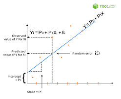
The inference method adopted in this book is mainly based on the likelihood function. The purpose of this section is to introduce vector space decompositions and show their roles when estimating parameters. In Appendix B, Theorems B.3 and B.11, a few important results about the linear space $\mathcal{C}(\bullet)$, its orthogonal complement $\mathcal{C}(\bullet)^{\perp}$ and projections $\boldsymbol{P}_A=\boldsymbol{A}\left(\boldsymbol{A}^{\prime} \boldsymbol{A}\right)^{-} \boldsymbol{A}^{\prime}$ are presented. Once again the univariate linear model
$$
\boldsymbol{x}^{\prime}=\boldsymbol{\beta}^{\prime} \boldsymbol{C}+\boldsymbol{e}^{\prime}, \quad \boldsymbol{e} \sim N_n\left(\mathbf{0}, \sigma^2 \boldsymbol{I}\right) .
$$ will be studied. In Example $1.1$ it was noted that $\widehat{\boldsymbol{\mu}}^{\prime}=\widehat{\boldsymbol{\beta}}^{\prime} \boldsymbol{C}$ and the maximum likelihood estimator of $\sigma^2$ equalled $n \widehat{\sigma}^2=\boldsymbol{r}^{\prime} \boldsymbol{r}$, where the “mean” $\widehat{\boldsymbol{\mu}}=\boldsymbol{P}{C^{\prime}} \boldsymbol{x}$ and “residuals” $\boldsymbol{r}=\left(\boldsymbol{I}-\boldsymbol{P}{C^{\prime}}\right) \boldsymbol{x}$. Hence, the estimators and residuals are obtained by projecting $\boldsymbol{x}$ on the column space $\mathcal{C}\left(\boldsymbol{C}^{\prime}\right)$ and on its orthogonal complement $\mathcal{C}\left(\boldsymbol{C}^{\prime}\right)^{\perp}$, respectively. The estimates are obtained by replacing $\boldsymbol{x}$ by $\boldsymbol{x}o$ in the expressions given above. Moreover, under normality, $\widehat{\mu}$ and $r$ are independently distributed and constitute the building blocks of the complete and sufficient statistics. Thus, $\widehat{\mu}$ and $\boldsymbol{r}$ are very fundamental quantities for carrying out inference according to the statistical paradigm, i.e. parameter estimation and model evaluation. Indeed, this is the basic philosophy adopted throughout this book, even if the models presented later become much more complicated. Consequently, the following space decomposition is of interest: $$ \mathcal{R}^n=\mathcal{C}\left(\boldsymbol{C}^{\prime}\right) \boxplus \mathcal{C}\left(\boldsymbol{C}^{\prime}\right)^{\perp}, $$ where $\boxplus$ denotes the orthogonal sum (see Appendix A, Sect. A.8), which is illustrated in Fig. 2.1. Suppose now that in the model $\boldsymbol{x}^{\prime}=\boldsymbol{\beta}^{\prime} \boldsymbol{C}+\boldsymbol{e}^{\prime}$, the restrictions $$ \beta^{\prime} \boldsymbol{G}=\mathbf{0} $$ hold. The restrictions mean that there is some prior information about $\boldsymbol{\beta}$ or some hypothesis has been postulated about the parameters in $\beta$. Then it follows from Sect. $1.3$ that $$ \widehat{\boldsymbol{\beta}}^{\prime} \boldsymbol{C}=\boldsymbol{x}^{\prime} \boldsymbol{C}^{\prime} \boldsymbol{G}^o\left(\boldsymbol{G}^{o^{\prime}} \boldsymbol{C} \boldsymbol{C}^{\prime} \boldsymbol{G}^o\right)^{-} \boldsymbol{G}^{o^{\prime}} \boldsymbol{C}=\boldsymbol{x}^{\prime} \boldsymbol{P}{C^{\prime} G^a}
$$

统计代写|回归分析作业代写Regression Analysis代考|Multivariate Linear Models

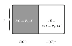
In this short section, an MLE for $\boldsymbol{\Sigma}$ is additionally given, for comparisons with the estimator of the variance in univariate linear models (see Fig. 2.5). The purpose of this section is to link univariate linear models with multivariate linear models, which will later be linked to the $B R M$. The multivariate linear model was presented in Sect. $1.4$ and its MLEs were given by
$$
\begin{aligned}
\widehat{\boldsymbol{B}}o \boldsymbol{C} & =\boldsymbol{X}_o \boldsymbol{P}{C^{\prime}}, \
n \widehat{\boldsymbol{\Sigma}}o & =\boldsymbol{r}_o \boldsymbol{r}_o^{\prime}, \quad \boldsymbol{r}_o^{\prime}=\left(\boldsymbol{I}-\boldsymbol{P}{C^{\prime}}\right) \boldsymbol{X}_o^{\prime} .
\end{aligned}
$$
In comparison with univariate linear models, the only difference when estimating parameters is that instead of $\boldsymbol{x}^{\prime}: 1 \times n$, we have $\boldsymbol{X}: p \times n$. Thus, in some sense, from a mathematical point of view, the treatment of the univariate and multivariate models concerning estimation is the same. Indeed it would be mathematically more correct to say “linear multivariate model” instead of “multivariate linear model”. However, if one considers properties of the estimators, then differences appear. This is mainly due to the difference between the Wishart distribution and the $\chi^2$ distribution (see Appendix A, Sect. A.9, for definitions of the distributions). Moreover, from a practical point of view, since in the multivariate case one is dealing with several variables simultaneously, the data analysis also becomes more complicated. For example, dependencies among the variables have to be taken into account, which of course is not necessary in the univariate case. Obviously there are more questions which are to be considered in the multivariate model. The differences between the univariate linear and multivariate linear models are illustrated in Fig. 2.5.

It is worth noting that any multivariate linear model via a vectorization can be written as a univariate linear model. Consider the multivariate linear model
$$
\boldsymbol{X}=\boldsymbol{B} \boldsymbol{C}+\boldsymbol{E}, \quad \boldsymbol{E} \sim N_{p, n}(\mathbf{0}, \boldsymbol{\Sigma}, \boldsymbol{I}), \quad \boldsymbol{\Sigma}>0,
$$
which can also be written as follows:
$$
\operatorname{vec} \boldsymbol{X}=\left(\boldsymbol{C}^{\prime} \otimes \boldsymbol{I}\right) \operatorname{vec} \boldsymbol{B}+\boldsymbol{e}, \quad \boldsymbol{e} \sim N_{p n}(\mathbf{0}, \boldsymbol{I} \otimes \boldsymbol{\Sigma}), \quad \boldsymbol{\Sigma}>0 .
$$
However, stating that any one of the representations given above has some general advantages does not make sense from a statistical point of view. Finally, it is noted that a general inference strategy in multivariate analysis is to take an arbitrary linear combination of $\boldsymbol{X}$, let us say $\boldsymbol{I}^{\prime} \boldsymbol{X}$, leading to a univariate model, and then to try to choose in some sense the best $l$ (e.g. see Rao, 1973, Chapter 8).

统计代写|回归分析作业代写Regression Analysis代考|STA321

回归分析代写

统计代写|回归分析作业代写Regression Analysis代考|Linear Models with a Focus on the Singular Gauss-Markov Model

本书采用的推理方法主要是基于似然函数。本节的目的是介绍向量空间分解并展示它们在估计参数时的作用。在附录 B,定理 B.3 和 B.11 中,关于线性空间的几个重要结果 $\mathcal{C}(\bullet)$ ,它的正交补集 $\mathcal{C}(\bullet)^{\perp}$ 和预测 $\boldsymbol{P}_A=\boldsymbol{A}\left(\boldsymbol{A}^{\prime} \boldsymbol{A}\right)^{-} \boldsymbol{A}^{\prime}$ 被提出。再次单变量线性模型
$$
\boldsymbol{x}^{\prime}=\boldsymbol{\beta}^{\prime} \boldsymbol{C}+\boldsymbol{e}^{\prime}, \quad \boldsymbol{e} \sim N_n\left(\mathbf{0}, \sigma^2 \boldsymbol{I}\right) .
$$
将被研究。在示例中 $1.1$ 有人指出 $\widehat{\boldsymbol{\mu}}^{\prime}=\widehat{\boldsymbol{\beta}}^{\prime} \boldsymbol{C}$ 和最大似然估计 $\sigma^2$ 等于 $n \widehat{\sigma}^2=\boldsymbol{r}^{\prime} \boldsymbol{r}$ ,其中”均值” $\widehat{\boldsymbol{\mu}}=\boldsymbol{P} C^{\prime} \boldsymbol{x}$ 和”残差” $\boldsymbol{r}=\left(\boldsymbol{I}-\boldsymbol{P} C^{\prime}\right) \boldsymbol{x}$. 因此,估计量和残差是通过投影获得的 $\boldsymbol{x}$ 在列空间 $\mathcal{C}\left(\boldsymbol{C}^{\prime}\right)$ 及其 正交补集 $\mathcal{C}\left(\boldsymbol{C}^{\prime}\right)^{\perp}$ ,分别。估计是通过替换获得的 $\boldsymbol{x}$ 经过 $\boldsymbol{x} o$ 在上面给出的表达式中。而且,在常态下, $\widehat{\mu}$ 和 $r$ 是独立分布的,构成了完整和充分统计的基石。因此, $\widehat{\mu}$ 和 $\boldsymbol{r}$ 是根据统计范式进行推理的非常基本的 量,即参数估计和模型评估。事实上,这就是贯穿本书的基本理念,即使后面介绍的模型变得更加复杂。 因此,以下空间分解很有趣:
$$
\mathcal{R}^n=\mathcal{C}\left(\boldsymbol{C}^{\prime}\right) \boxplus \mathcal{C}\left(\boldsymbol{C}^{\prime}\right)^{\perp},
$$
在哪里田表示正交和(参见附录 A,A.8 节) ,如图 $2.1$ 所示。现在假设在模型中 $\boldsymbol{x}^{\prime}=\boldsymbol{\beta}^{\prime} \boldsymbol{C}+\boldsymbol{e}^{\prime}$ ,限制
$$
\beta^{\prime} \boldsymbol{G}=\mathbf{0}
$$
抓住。这些限制意味着有一些先验信息 $\beta$ 或者已经假设了关于参数的一些假设 $\beta$. 然后它来自 Sect。1.3那
$$
\widehat{\boldsymbol{\beta}}^{\prime} \boldsymbol{C}=\boldsymbol{x}^{\prime} \boldsymbol{C}^{\prime} \boldsymbol{G}^o\left(\boldsymbol{G}^{o^{\prime}} \boldsymbol{C} \boldsymbol{C}^{\prime} \boldsymbol{G}^o\right)^{-} \boldsymbol{G}^{o^{\prime}} \boldsymbol{C}=\boldsymbol{x}^{\prime} \boldsymbol{P} C^{\prime} G^a
$$

统计代写|回归分析作业代写Regression Analysis代考|Multivariate Linear Models

在这个简短的部分中, MLE 用于 $\boldsymbol{\Sigma}$ 另外给出,用于与单变量线性模型中的方差估计量进行比较(见图 2.5)。本节的目的是将单变量线性模型与多元线性模型联系起来,稍后将链接到 $B R M$. 多元线性模型 在第 1 节中介绍。1.4其 MLE 由
$$
\widehat{\boldsymbol{B}} o \boldsymbol{C}=\boldsymbol{X}o \boldsymbol{P} C^{\prime}, n \widehat{\boldsymbol{\Sigma}} o \quad=\boldsymbol{r}_o \boldsymbol{r}_o^{\prime}, \quad \boldsymbol{r}_o^{\prime}=\left(\boldsymbol{I}-\boldsymbol{P} C^{\prime}\right) \boldsymbol{X}_o^{\prime} . $$ 与单变量线性模型相比,估计参数时的唯一区别是,而不是 $\boldsymbol{x}^{\prime}: 1 \times n$ ,我们有 $\boldsymbol{X}: p \times n$. 因此,从某 种意义上说,从数学的角度来看,单变量模型和多变量模型在估计方面的处理是相同的。实际上,说 线 性多元模型”而不是“多元线性模型”在数学上更正确。但是,如果考虑估计量的属性,就会出现差异。这主 要是由于 Wishart 分布和 $\chi^2$ 分布(有关分布的定义,请参阅附录 A,第 A.9 节) 。而且,从实际的角度 来看,由于在多变量情况下同时处理多个变量,数据分析也变得更加复杂。例如,必须考虑变量之间的依 赖关系,这在单变量情况下当然是不必要的。显然,多元模型需要考虑的问题更多。单变量线性模型和多 变量线性模型之间的差异如图 $2.5$ 所示。 值得注意的是,任何通过向量化的多元线性模型都可以写成单变量线性模型。考虑多元线性模型 $$ \boldsymbol{X}=\boldsymbol{B} \boldsymbol{C}+\boldsymbol{E}, \quad \boldsymbol{E} \sim N{p, n}(\mathbf{0}, \mathbf{\Sigma}, \boldsymbol{I}), \quad \mathbf{\Sigma}>0,
$$
也可以这样写:
$$
\operatorname{vec} \boldsymbol{X}=\left(\boldsymbol{C}^{\prime} \otimes \boldsymbol{I}\right) \operatorname{vec} \boldsymbol{B}+\boldsymbol{e}, \quad \boldsymbol{e} \sim N_{p n}(\mathbf{0}, \boldsymbol{I} \otimes \mathbf{\Sigma}), \quad \boldsymbol{\Sigma}>0 .
$$
然而,从统计的角度来看,声明上面给出的任何一种表示具有一些普遍优势是没有意义的。最后,值得注 意的是,多元分析中的一般推理策略是乎用任意线性组合 $\boldsymbol{X}$ ,让我们说 $\boldsymbol{I}^{\prime} \boldsymbol{X}$ ,导致单变量模型,然后尝 试在某种意义上选择最好的 $l$ (例如参见 Rao,1973 年,第 8 章)。

统计代写|回归分析作业代写Regression Analysis代考 请认准statistics-lab™

统计代写请认准statistics-lab™. statistics-lab™为您的留学生涯保驾护航。

随机过程代考

在概率论概念中,随机过程随机变量的集合。 若一随机系统的样本点是随机函数,则称此函数为样本函数,这一随机系统全部样本函数的集合是一个随机过程。 实际应用中,样本函数的一般定义在时间域或者空间域。 随机过程的实例如股票和汇率的波动、语音信号、视频信号、体温的变化,随机运动如布朗运动、随机徘徊等等。

贝叶斯方法代考

贝叶斯统计概念及数据分析表示使用概率陈述回答有关未知参数的研究问题以及统计范式。后验分布包括关于参数的先验分布,和基于观测数据提供关于参数的信息似然模型。根据选择的先验分布和似然模型,后验分布可以解析或近似,例如,马尔科夫链蒙特卡罗 (MCMC) 方法之一。贝叶斯统计概念及数据分析使用后验分布来形成模型参数的各种摘要,包括点估计,如后验平均值、中位数、百分位数和称为可信区间的区间估计。此外,所有关于模型参数的统计检验都可以表示为基于估计后验分布的概率报表。

广义线性模型代考

广义线性模型(GLM)归属统计学领域,是一种应用灵活的线性回归模型。该模型允许因变量的偏差分布有除了正态分布之外的其它分布。

statistics-lab作为专业的留学生服务机构,多年来已为美国、英国、加拿大、澳洲等留学热门地的学生提供专业的学术服务,包括但不限于Essay代写,Assignment代写,Dissertation代写,Report代写,小组作业代写,Proposal代写,Paper代写,Presentation代写,计算机作业代写,论文修改和润色,网课代做,exam代考等等。写作范围涵盖高中,本科,研究生等海外留学全阶段,辐射金融,经济学,会计学,审计学,管理学等全球99%专业科目。写作团队既有专业英语母语作者,也有海外名校硕博留学生,每位写作老师都拥有过硬的语言能力,专业的学科背景和学术写作经验。我们承诺100%原创,100%专业,100%准时,100%满意。

机器学习代写

随着AI的大潮到来,Machine Learning逐渐成为一个新的学习热点。同时与传统CS相比,Machine Learning在其他领域也有着广泛的应用,因此这门学科成为不仅折磨CS专业同学的“小恶魔”,也是折磨生物、化学、统计等其他学科留学生的“大魔王”。学习Machine learning的一大绊脚石在于使用语言众多,跨学科范围广,所以学习起来尤其困难。但是不管你在学习Machine Learning时遇到任何难题,StudyGate专业导师团队都能为你轻松解决。

多元统计分析代考


基础数据: $N$ 个样本, $P$ 个变量数的单样本,组成的横列的数据表
变量定性: 分类和顺序;变量定量:数值
数学公式的角度分为: 因变量与自变量

时间序列分析代写

随机过程,是依赖于参数的一组随机变量的全体,参数通常是时间。 随机变量是随机现象的数量表现,其时间序列是一组按照时间发生先后顺序进行排列的数据点序列。通常一组时间序列的时间间隔为一恒定值(如1秒,5分钟,12小时,7天,1年),因此时间序列可以作为离散时间数据进行分析处理。研究时间序列数据的意义在于现实中,往往需要研究某个事物其随时间发展变化的规律。这就需要通过研究该事物过去发展的历史记录,以得到其自身发展的规律。

回归分析代写

多元回归分析渐进(Multiple Regression Analysis Asymptotics)属于计量经济学领域,主要是一种数学上的统计分析方法,可以分析复杂情况下各影响因素的数学关系,在自然科学、社会和经济学等多个领域内应用广泛。

MATLAB代写

MATLAB 是一种用于技术计算的高性能语言。它将计算、可视化和编程集成在一个易于使用的环境中,其中问题和解决方案以熟悉的数学符号表示。典型用途包括:数学和计算算法开发建模、仿真和原型制作数据分析、探索和可视化科学和工程图形应用程序开发,包括图形用户界面构建MATLAB 是一个交互式系统,其基本数据元素是一个不需要维度的数组。这使您可以解决许多技术计算问题,尤其是那些具有矩阵和向量公式的问题,而只需用 C 或 Fortran 等标量非交互式语言编写程序所需的时间的一小部分。MATLAB 名称代表矩阵实验室。MATLAB 最初的编写目的是提供对由 LINPACK 和 EISPACK 项目开发的矩阵软件的轻松访问,这两个项目共同代表了矩阵计算软件的最新技术。MATLAB 经过多年的发展,得到了许多用户的投入。在大学环境中,它是数学、工程和科学入门和高级课程的标准教学工具。在工业领域,MATLAB 是高效研究、开发和分析的首选工具。MATLAB 具有一系列称为工具箱的特定于应用程序的解决方案。对于大多数 MATLAB 用户来说非常重要,工具箱允许您学习应用专业技术。工具箱是 MATLAB 函数(M 文件)的综合集合,可扩展 MATLAB 环境以解决特定类别的问题。可用工具箱的领域包括信号处理、控制系统、神经网络、模糊逻辑、小波、仿真等。

R语言代写问卷设计与分析代写
PYTHON代写回归分析与线性模型代写
MATLAB代写方差分析与试验设计代写
STATA代写机器学习/统计学习代写
SPSS代写计量经济学代写
EVIEWS代写时间序列分析代写
EXCEL代写深度学习代写
SQL代写各种数据建模与可视化代写

统计代写|回归分析作业代写Regression Analysis代考|STA4210

如果你也在 怎样代写回归分析Regression Analysis这个学科遇到相关的难题,请随时右上角联系我们的24/7代写客服。

回归分析是一种强大的统计方法,允许你检查两个或多个感兴趣的变量之间的关系。虽然有许多类型的回归分析,但它们的核心都是考察一个或多个自变量对因变量的影响。

statistics-lab™ 为您的留学生涯保驾护航 在代写回归分析Regression Analysis方面已经树立了自己的口碑, 保证靠谱, 高质且原创的统计Statistics代写服务。我们的专家在代写回归分析Regression Analysis代写方面经验极为丰富,各种代写回归分析Regression Analysis相关的作业也就用不着说。

我们提供的回归分析Regression Analysis及其相关学科的代写,服务范围广, 其中包括但不限于:

  • Statistical Inference 统计推断
  • Statistical Computing 统计计算
  • Advanced Probability Theory 高等楖率论
  • Advanced Mathematical Statistics 高等数理统计学
  • (Generalized) Linear Models 广义线性模型
  • Statistical Machine Learning 统计机器学习
  • Longitudinal Data Analysis 纵向数据分析
  • Foundations of Data Science 数据科学基础
统计代写|回归分析作业代写Regression Analysis代考|STA4210

统计代写|回归分析作业代写Regression Analysis代考|How Strong of a Correlation is Considered Good

What is a good correlation? How high should it be? These are commonly asked questions. I have seen several schemes that attempt to classify correlations as strong, medium, and weak.

However, there is only one correct answer. The correlation coefficient should accurately reflect the strength of the relationship. Take a look at the correlation between the height and weight data, $0.705$. It’s not a very strong relationship, but it accurately represents our data.

An accurate representation is the best-case scenario for using a statistic to describe an entire dataset.

The strength of any relationship naturally depends on the specific pair of variables. Some research questions involve weaker relationships than other subject areas. Case in point, humans are hard to predict. Studies that assess relationships involving human behavior tend to have correlations weaker than $+/-0.6$.

However, if you analyze two variables in a physical process, and have very precise measurements, you might expect correlations near $+1$ or $-1$. There is no one-size fits all best answer for how strong a relationship should be. The correct correlation value depends on your study area. We run into this same issue in regression analysis.

统计代写|回归分析作业代写Regression Analysis代考|Common Themes with Regression

Understanding correlation is a good place to start learning regression. In fact, there are several themes that I touch upon in this section that show up throughout this book.

For instance, analysts naturally want to fit models that explain more and more of the variability in the data. And, they come up with classification schemes for how well the model fits the data. However, there is a natural amount of variability that the model can’t explain just as there was in the height and weight correlation example. Regression models can be forced to go past this natural boundary, but bad things happen. Throughout this book, be aware of the tension between trying to explain as much variability as possible and ensuring that you don’t go too far. This issue pops up multiple times!

Additionally, for regression analysis, you’ll need to use statistical measures in conjunction with graphs just like we did with correlation. This combination provides you the best understanding of your data and the analytical results.

Wouldn’t it be nice if instead of just describing the strength of the relationship between height and weight, we could define the relationship itself using an equation? Regression analysis does just that by finding the line and corresponding equation that provides the best fit to our dataset. We can use that equation to understand how much weight increases with each additional unit of height and to make predictions for specific heights.

Regression analysis allows us to expand on correlation in other ways. If we have more variables that explain changes in weight, we can include them in the model and potentially improve our predictions. And, if the relationship is curved, we can still fit a regression model to the data.

Additionally, a form of the Pearson correlation coefficient shows up in regression analysis. R-squared is a primary measure of how well a regression model fits the data. This statistic represents the percentage of variation in one variable that other variables explain. For a pair of variables, R-squared is simply the square of the Pearson’s correlation coefficient. For example, squaring the height-weight correlation coefficient of $0.705$ produces an R-squared of $0.497$, or $49.7 \%$. In other words, height explains about half the variability of weight in preteen girls.

But we’re getting ahead of ourselves. I’ll cover R-squared in much more detail in both chapters 2 and 4.

统计代写|回归分析作业代写Regression Analysis代考|STA4210

回归分析代写

统计代写|回归分析作业代写Regression Analysis代考|How Strong of a Correlation is Considered Good

什么是好的相关性?应该多高?这些是常见问题。我见过几种试图将相关性分类为强、中和弱的方案。

然而,只有一个正确答案。相关系数应准确反映关系的强度。看一下身高体重数据的相关性,0.705. 这不是一个很强的关系,但它准确地代表了我们的数据。

准确的表示是使用统计数据描述整个数据集的最佳情况。

任何关系的强度自然取决于特定的变量对。一些研究问题涉及比其他学科领域更弱的关系。举个例子,人类很难预测。评估涉及人类行为的关系的研究往往具有比+/−0.6.

但是,如果您分析一个物理过程中的两个变量,并进行非常精确的测量,您可能会期望相关性接近+1或者−1. 对于一段关系应该有多牢固,没有一个千篇一律的最佳答案。正确的相关值取决于您的研究区域。我们在回归分析中遇到了同样的问题。

统计代写|回归分析作业代写Regression Analysis代考|Common Themes with Regression

了解相关性是开始学习回归的好地方。事实上,我在本节中涉及的几个主题贯穿全书。

例如,分析师自然希望拟合能够解释越来越多的数据可变性的模型。并且,他们针对模型与数据的拟合程度提出了分类方案。但是,存在模型无法解释的自然变异量,就像身高和体重相关性示例中那样。回归模型可能会被迫越过这个自然边界,但坏事还是会发生。在整本书中,请注意试图解释尽可能多的可变性与确保您不会走得太远之间的紧张关系。这个问题多次出现!

此外,对于回归分析,您需要将统计指标与图表结合使用,就像我们处理相关性一样。这种组合可以让您更好地理解您的数据和分析结果。

如果我们不仅可以描述身高和体重之间关系的强度,还可以使用方程式来定义关系本身,那岂不是很好?回归分析通过找到最适合我们的数据集的直线和相应的方程来做到这一点。我们可以使用该等式来了解每增加一个单位的身高体重会增加多少,并预测特定的身高。

回归分析使我们能够以其他方式扩展相关性。如果我们有更多的变量来解释体重的变化,我们可以将它们包含在模型中,并有可能改进我们的预测。而且,如果关系是弯曲的,我们仍然可以对数据拟合回归模型。

此外,皮尔逊相关系数的一种形式出现在回归分析中。R 平方是衡量回归模型与数据拟合程度的主要指标。此统计数据表示其他变量解释的一个变量的变化百分比。对于一对变量,R 平方就是 Pearson 相关系数的平方。例如,将身高体重相关系数平方0.705产生一个 R 平方0.497, 或者49.7%. 换句话说,身高解释了青春期前女孩大约一半的体重变化。

但我们已经超前了。我将在第 2 章和第 4 章中更详细地介绍 R 平方。

统计代写|回归分析作业代写Regression Analysis代考 请认准statistics-lab™

统计代写请认准statistics-lab™. statistics-lab™为您的留学生涯保驾护航。

随机过程代考

在概率论概念中,随机过程随机变量的集合。 若一随机系统的样本点是随机函数,则称此函数为样本函数,这一随机系统全部样本函数的集合是一个随机过程。 实际应用中,样本函数的一般定义在时间域或者空间域。 随机过程的实例如股票和汇率的波动、语音信号、视频信号、体温的变化,随机运动如布朗运动、随机徘徊等等。

贝叶斯方法代考

贝叶斯统计概念及数据分析表示使用概率陈述回答有关未知参数的研究问题以及统计范式。后验分布包括关于参数的先验分布,和基于观测数据提供关于参数的信息似然模型。根据选择的先验分布和似然模型,后验分布可以解析或近似,例如,马尔科夫链蒙特卡罗 (MCMC) 方法之一。贝叶斯统计概念及数据分析使用后验分布来形成模型参数的各种摘要,包括点估计,如后验平均值、中位数、百分位数和称为可信区间的区间估计。此外,所有关于模型参数的统计检验都可以表示为基于估计后验分布的概率报表。

广义线性模型代考

广义线性模型(GLM)归属统计学领域,是一种应用灵活的线性回归模型。该模型允许因变量的偏差分布有除了正态分布之外的其它分布。

statistics-lab作为专业的留学生服务机构,多年来已为美国、英国、加拿大、澳洲等留学热门地的学生提供专业的学术服务,包括但不限于Essay代写,Assignment代写,Dissertation代写,Report代写,小组作业代写,Proposal代写,Paper代写,Presentation代写,计算机作业代写,论文修改和润色,网课代做,exam代考等等。写作范围涵盖高中,本科,研究生等海外留学全阶段,辐射金融,经济学,会计学,审计学,管理学等全球99%专业科目。写作团队既有专业英语母语作者,也有海外名校硕博留学生,每位写作老师都拥有过硬的语言能力,专业的学科背景和学术写作经验。我们承诺100%原创,100%专业,100%准时,100%满意。

机器学习代写

随着AI的大潮到来,Machine Learning逐渐成为一个新的学习热点。同时与传统CS相比,Machine Learning在其他领域也有着广泛的应用,因此这门学科成为不仅折磨CS专业同学的“小恶魔”,也是折磨生物、化学、统计等其他学科留学生的“大魔王”。学习Machine learning的一大绊脚石在于使用语言众多,跨学科范围广,所以学习起来尤其困难。但是不管你在学习Machine Learning时遇到任何难题,StudyGate专业导师团队都能为你轻松解决。

多元统计分析代考


基础数据: $N$ 个样本, $P$ 个变量数的单样本,组成的横列的数据表
变量定性: 分类和顺序;变量定量:数值
数学公式的角度分为: 因变量与自变量

时间序列分析代写

随机过程,是依赖于参数的一组随机变量的全体,参数通常是时间。 随机变量是随机现象的数量表现,其时间序列是一组按照时间发生先后顺序进行排列的数据点序列。通常一组时间序列的时间间隔为一恒定值(如1秒,5分钟,12小时,7天,1年),因此时间序列可以作为离散时间数据进行分析处理。研究时间序列数据的意义在于现实中,往往需要研究某个事物其随时间发展变化的规律。这就需要通过研究该事物过去发展的历史记录,以得到其自身发展的规律。

回归分析代写

多元回归分析渐进(Multiple Regression Analysis Asymptotics)属于计量经济学领域,主要是一种数学上的统计分析方法,可以分析复杂情况下各影响因素的数学关系,在自然科学、社会和经济学等多个领域内应用广泛。

MATLAB代写

MATLAB 是一种用于技术计算的高性能语言。它将计算、可视化和编程集成在一个易于使用的环境中,其中问题和解决方案以熟悉的数学符号表示。典型用途包括:数学和计算算法开发建模、仿真和原型制作数据分析、探索和可视化科学和工程图形应用程序开发,包括图形用户界面构建MATLAB 是一个交互式系统,其基本数据元素是一个不需要维度的数组。这使您可以解决许多技术计算问题,尤其是那些具有矩阵和向量公式的问题,而只需用 C 或 Fortran 等标量非交互式语言编写程序所需的时间的一小部分。MATLAB 名称代表矩阵实验室。MATLAB 最初的编写目的是提供对由 LINPACK 和 EISPACK 项目开发的矩阵软件的轻松访问,这两个项目共同代表了矩阵计算软件的最新技术。MATLAB 经过多年的发展,得到了许多用户的投入。在大学环境中,它是数学、工程和科学入门和高级课程的标准教学工具。在工业领域,MATLAB 是高效研究、开发和分析的首选工具。MATLAB 具有一系列称为工具箱的特定于应用程序的解决方案。对于大多数 MATLAB 用户来说非常重要,工具箱允许您学习应用专业技术。工具箱是 MATLAB 函数(M 文件)的综合集合,可扩展 MATLAB 环境以解决特定类别的问题。可用工具箱的领域包括信号处理、控制系统、神经网络、模糊逻辑、小波、仿真等。

R语言代写问卷设计与分析代写
PYTHON代写回归分析与线性模型代写
MATLAB代写方差分析与试验设计代写
STATA代写机器学习/统计学习代写
SPSS代写计量经济学代写
EVIEWS代写时间序列分析代写
EXCEL代写深度学习代写
SQL代写各种数据建模与可视化代写

统计代写|回归分析作业代写Regression Analysis代考|STAT2220

如果你也在 怎样代写回归分析Regression Analysis这个学科遇到相关的难题,请随时右上角联系我们的24/7代写客服。

回归分析是一种强大的统计方法,允许你检查两个或多个感兴趣的变量之间的关系。虽然有许多类型的回归分析,但它们的核心都是考察一个或多个自变量对因变量的影响。

statistics-lab™ 为您的留学生涯保驾护航 在代写回归分析Regression Analysis方面已经树立了自己的口碑, 保证靠谱, 高质且原创的统计Statistics代写服务。我们的专家在代写回归分析Regression Analysis代写方面经验极为丰富,各种代写回归分析Regression Analysis相关的作业也就用不着说。

我们提供的回归分析Regression Analysis及其相关学科的代写,服务范围广, 其中包括但不限于:

  • Statistical Inference 统计推断
  • Statistical Computing 统计计算
  • Advanced Probability Theory 高等楖率论
  • Advanced Mathematical Statistics 高等数理统计学
  • (Generalized) Linear Models 广义线性模型
  • Statistical Machine Learning 统计机器学习
  • Longitudinal Data Analysis 纵向数据分析
  • Foundations of Data Science 数据科学基础
统计代写|回归分析作业代写Regression Analysis代考|STAT2220

统计代写|回归分析作业代写Regression Analysis代考|Hypothesis Test for Correlations

Correlations have a hypothesis test. As with any hypothesis test, this test takes sample data and evaluates two mutually exclusive statements about the population from which the sample was drawn. For Pearson correlations, the two hypotheses are the following:

  • Null hypothesis: There is no linear relationship between the two variables. $\rho=0$.
  • Alternative hypothesis: There is a linear relationship between the two variables. $\rho \neq 0$.

A correlation of zero indicates that no linear relationship exists. If your p-value is less than your significance level, the sample contains sufficient evidence to reject the null hypothesis and conclude that the correlation does not equal zero. In other words, the sample data support the notion that the relationship exists in the population.

Now that we have seen a range of positive and negative relationships, let’s see how our correlation of $0.705$ fits in. We know that it’s a positive relationship. As height increases, weight tends to increase. Regarding the strength of the relationship, the graph shows that it’s not a very strong relationship where the data points tightly hug a line. However, it’s not an entirely amorphous blob with a very low correlation. It’s somewhere in between. That description matches our moderate correlation of $0.705$.

For the hypothesis test, our p-value equals $0.000$. This p-value is less than any reasonable significance level. Consequently, we can reject the null hypothesis and conclude that the relationship is statistically significant. The sample data provide sufficient evidence to conclude that the relationship between height and weight exists in the population of preteen girls.

统计代写|回归分析作业代写Regression Analysis代考|Correlation Does Not Imply Causation

I’m sure you’ve heard this expression before, and it is a crucial warning. Correlation between two variables indicates that changes in one variable are associated with changes in the other variable. However, correlation does not mean that the changes in one variable actually cause the changes in the other variable.

Sometimes it is clear that there is a causal relationship. For the height and weight data, it makes sense that adding more vertical structure to a body causes the total mass to increase. Or, increasing the wattage of lightbulbs causes the light output to increase.

However, in other cases, a causal relationship is not possible. For example, ice cream sales and shark attacks are positively correlated. Clearly, selling more ice cream does not cause shark attacks (or vice versa). Instead, a third variable, outdoor temperatures, causes changes in the other two variables. Higher temperatures increase both sales of ice cream and the number of swimmers in the ocean, which creates the apparent relationship between ice cream sales and shark attacks.
In statistics, you typically need to perform a randomized, controlled experiment to determine that a relationship is causal rather than merely correlation.

统计代写|回归分析作业代写Regression Analysis代考|STAT2220

回归分析代写

统计代写|回归分析作业代写Regression Analysis代考|Hypothesis Test for Correlations

相关性有一个假设检验。与任何假设检验一样,此检验获取样本数据并评估关于抽取样本的总体的两个相互排斥的陈述。对于 Pearson 相关性,两个假设如下:

  • 零假设:两个变量之间不存在线性关系。r=0.
  • 备择假设:两个变量之间存在线性关系。r≠0.

相关性为零表示不存在线性关系。如果您的 p 值小于您的显着性水平,则样本包含足够的证据来拒绝原假设并得出相关性不为零的结论。换句话说,样本数据支持人口中存在关系的概念。

现在我们已经看到了一系列积极和消极的关系,让我们看看我们的相关性0.705适合。我们知道这是一种积极的关系。随着身高的增加,体重往往会增加。关于关系的强度,该图显示数据点紧靠一条线的关系不是很强。然而,它并不是一个相关性非常低的完全无定形的斑点。它介于两者之间。该描述符合我们的适度相关性0.705.

对于假设检验,我们的 p 值等于0.000. 此 p 值小于任何合理的显着性水平。因此,我们可以拒绝零假设并得出结论,该关系具有统计显着性。样本数据提供了充分的证据,可以得出青春期前女孩人群中身高和体重之间存在关系的结论。

统计代写|回归分析作业代写Regression Analysis代考|Correlation Does Not Imply Causation

我相信你以前听过这个表达,这是一个重要的警告。两个变量之间的相关性表明一个变量的变化与另一个变量的变化相关联。但是,相关性并不意味着一个变量的变化实际上会导致另一个变量的变化。

有时很明显存在因果关系。对于身高和体重数据,向身体添加更多垂直结构会导致总质量增加是有道理的。或者,增加灯泡的瓦数会导致光输出增加。

但是,在其他情况下,因果关系是不可能的。例如,冰淇淋销售和鲨鱼袭击是正相关的。显然,销售更多冰淇淋不会导致鲨鱼袭击(反之亦然)。相反,第三个变量,即室外温度,会引起其他两个变量的变化。较高的温度会增加冰淇淋的销量和海中游泳者的数量,从而在冰淇淋销量和鲨鱼袭击之间建立明显的关系。
在统计学中,您通常需要执行随机对照实验来确定关系是因果关系而不仅仅是相关性。

统计代写|回归分析作业代写Regression Analysis代考 请认准statistics-lab™

统计代写请认准statistics-lab™. statistics-lab™为您的留学生涯保驾护航。

随机过程代考

在概率论概念中,随机过程随机变量的集合。 若一随机系统的样本点是随机函数,则称此函数为样本函数,这一随机系统全部样本函数的集合是一个随机过程。 实际应用中,样本函数的一般定义在时间域或者空间域。 随机过程的实例如股票和汇率的波动、语音信号、视频信号、体温的变化,随机运动如布朗运动、随机徘徊等等。

贝叶斯方法代考

贝叶斯统计概念及数据分析表示使用概率陈述回答有关未知参数的研究问题以及统计范式。后验分布包括关于参数的先验分布,和基于观测数据提供关于参数的信息似然模型。根据选择的先验分布和似然模型,后验分布可以解析或近似,例如,马尔科夫链蒙特卡罗 (MCMC) 方法之一。贝叶斯统计概念及数据分析使用后验分布来形成模型参数的各种摘要,包括点估计,如后验平均值、中位数、百分位数和称为可信区间的区间估计。此外,所有关于模型参数的统计检验都可以表示为基于估计后验分布的概率报表。

广义线性模型代考

广义线性模型(GLM)归属统计学领域,是一种应用灵活的线性回归模型。该模型允许因变量的偏差分布有除了正态分布之外的其它分布。

statistics-lab作为专业的留学生服务机构,多年来已为美国、英国、加拿大、澳洲等留学热门地的学生提供专业的学术服务,包括但不限于Essay代写,Assignment代写,Dissertation代写,Report代写,小组作业代写,Proposal代写,Paper代写,Presentation代写,计算机作业代写,论文修改和润色,网课代做,exam代考等等。写作范围涵盖高中,本科,研究生等海外留学全阶段,辐射金融,经济学,会计学,审计学,管理学等全球99%专业科目。写作团队既有专业英语母语作者,也有海外名校硕博留学生,每位写作老师都拥有过硬的语言能力,专业的学科背景和学术写作经验。我们承诺100%原创,100%专业,100%准时,100%满意。

机器学习代写

随着AI的大潮到来,Machine Learning逐渐成为一个新的学习热点。同时与传统CS相比,Machine Learning在其他领域也有着广泛的应用,因此这门学科成为不仅折磨CS专业同学的“小恶魔”,也是折磨生物、化学、统计等其他学科留学生的“大魔王”。学习Machine learning的一大绊脚石在于使用语言众多,跨学科范围广,所以学习起来尤其困难。但是不管你在学习Machine Learning时遇到任何难题,StudyGate专业导师团队都能为你轻松解决。

多元统计分析代考


基础数据: $N$ 个样本, $P$ 个变量数的单样本,组成的横列的数据表
变量定性: 分类和顺序;变量定量:数值
数学公式的角度分为: 因变量与自变量

时间序列分析代写

随机过程,是依赖于参数的一组随机变量的全体,参数通常是时间。 随机变量是随机现象的数量表现,其时间序列是一组按照时间发生先后顺序进行排列的数据点序列。通常一组时间序列的时间间隔为一恒定值(如1秒,5分钟,12小时,7天,1年),因此时间序列可以作为离散时间数据进行分析处理。研究时间序列数据的意义在于现实中,往往需要研究某个事物其随时间发展变化的规律。这就需要通过研究该事物过去发展的历史记录,以得到其自身发展的规律。

回归分析代写

多元回归分析渐进(Multiple Regression Analysis Asymptotics)属于计量经济学领域,主要是一种数学上的统计分析方法,可以分析复杂情况下各影响因素的数学关系,在自然科学、社会和经济学等多个领域内应用广泛。

MATLAB代写

MATLAB 是一种用于技术计算的高性能语言。它将计算、可视化和编程集成在一个易于使用的环境中,其中问题和解决方案以熟悉的数学符号表示。典型用途包括:数学和计算算法开发建模、仿真和原型制作数据分析、探索和可视化科学和工程图形应用程序开发,包括图形用户界面构建MATLAB 是一个交互式系统,其基本数据元素是一个不需要维度的数组。这使您可以解决许多技术计算问题,尤其是那些具有矩阵和向量公式的问题,而只需用 C 或 Fortran 等标量非交互式语言编写程序所需的时间的一小部分。MATLAB 名称代表矩阵实验室。MATLAB 最初的编写目的是提供对由 LINPACK 和 EISPACK 项目开发的矩阵软件的轻松访问,这两个项目共同代表了矩阵计算软件的最新技术。MATLAB 经过多年的发展,得到了许多用户的投入。在大学环境中,它是数学、工程和科学入门和高级课程的标准教学工具。在工业领域,MATLAB 是高效研究、开发和分析的首选工具。MATLAB 具有一系列称为工具箱的特定于应用程序的解决方案。对于大多数 MATLAB 用户来说非常重要,工具箱允许您学习应用专业技术。工具箱是 MATLAB 函数(M 文件)的综合集合,可扩展 MATLAB 环境以解决特定类别的问题。可用工具箱的领域包括信号处理、控制系统、神经网络、模糊逻辑、小波、仿真等。

R语言代写问卷设计与分析代写
PYTHON代写回归分析与线性模型代写
MATLAB代写方差分析与试验设计代写
STATA代写机器学习/统计学习代写
SPSS代写计量经济学代写
EVIEWS代写时间序列分析代写
EXCEL代写深度学习代写
SQL代写各种数据建模与可视化代写

统计代写|回归分析作业代写Regression Analysis代考|STA321

如果你也在 怎样代写回归分析Regression Analysis这个学科遇到相关的难题,请随时右上角联系我们的24/7代写客服。

回归分析是一种强大的统计方法,允许你检查两个或多个感兴趣的变量之间的关系。虽然有许多类型的回归分析,但它们的核心都是考察一个或多个自变量对因变量的影响。

statistics-lab™ 为您的留学生涯保驾护航 在代写回归分析Regression Analysis方面已经树立了自己的口碑, 保证靠谱, 高质且原创的统计Statistics代写服务。我们的专家在代写回归分析Regression Analysis代写方面经验极为丰富,各种代写回归分析Regression Analysis相关的作业也就用不着说。

我们提供的回归分析Regression Analysis及其相关学科的代写,服务范围广, 其中包括但不限于:

  • Statistical Inference 统计推断
  • Statistical Computing 统计计算
  • Advanced Probability Theory 高等楖率论
  • Advanced Mathematical Statistics 高等数理统计学
  • (Generalized) Linear Models 广义线性模型
  • Statistical Machine Learning 统计机器学习
  • Longitudinal Data Analysis 纵向数据分析
  • Foundations of Data Science 数据科学基础
统计代写|回归分析作业代写Regression Analysis代考|STA321

统计代写|回归分析作业代写Regression Analysis代考|Interpret the Pearson’s Correlation Coefficient

What do the correlation and p-value mean? We’ll interpret the output soon. First, let’s look at a range of possible correlation values so we can understand how our height and weight example fits in.

Pearson’s correlation coefficient is represented by the Greek letter rho ( $\rho$ ) for the population parameter and $r$ for a sample statistic. This coefficient is a single number that measures both the strength and direction of the linear relationship between two continuous variables. Values can range from $-1$ to $+1$.

  • Strength: The greater the absolute value of the coefficient, the stronger the relationship.
  • The extreme values of $-1$ and 1 indicate a perfectly linear relationship where a change in one variable is accompanied by a perfectly consistent change in the other. For these relationships, all of the data points fall on a line. In practice, you won’t see either type of perfect relationship. A coefficient of zero represents no linear relationship. As one variable increases, there is no tendency in the other variable to either increase or decrease.
  • When the value is in-between 0 and $+1 /-1$, there is a relationship, but the points don’t all fall on a line. As $r$

approaches $-1$ or 1 , the strength of the relationship increases and the data points tend to fall closer to a line.

  • Direction: The coefficient sign represents the direction of the relationship.
  • Positive coefficients indicate that when the value of one variable increases, the value of the other variable also tends to increase. Positive relationships produce an upward slope on a scatterplot.
  • Negative coefficients represent cases when the value of one variable increases, the value of the other variable tends to decrease. Negative relationships produce a downward slope.
    Examples of Positive and Negative Correlations
    An example of a positive correlation is the relationship between the speed of a wind turbine and the amount of energy it produces. As the turbine speed increases, electricity production also increases.

An example of a negative correlation is the relationship between outdoor temperature and heating costs. As the temperature increases, heating costs decrease.

统计代写|回归分析作业代写Regression Analysis代考|Discussion about the Correlation Scatterplots

For the scatterplots above, I created one positive relationship between the variables and one negative relationship between the variables. Then, I varied only the amount of dispersion between the data points and the line that defines the relationship. That process illustrates how correlation measures the strength of the relationship. The stronger the relationship, the closer the data points fall to the line. I didn’t include plots for weaker correlations that are closer to zero than $0.6$ and $-0.6$ because they start to look like blobs of dots and it’s hard to see the relationship.

A common misinterpretation is that a negative correlation coefficient indicates there is no relationship between a pair of variables. After all, a negative correlation sounds suspiciously like no relationship. However, the scatterplots for the negative correlations display real relationships. For negative relationships, high values of one variable are associated with low values of another variable. For example, there is a negative correlation between school absences and grades. As the number of absences increases, the grades decrease.

Earlier I mentioned how crucial it is to graph your data to understand them better. However, a quantitative assessment of the relationship does have an advantage. Graphs are a great way to visualize the data, but the scaling can exaggerate or weaken the appearance of a relationship. Additionally, the automatic scaling in most statistical software tends to make all data look similar.

Fortunately, Pearson’s correlation coefficient is unaffected by scaling issues. Consequently, a statistical assessment is better for determining the precise strength of the relationship.

Graphs and the relevant statistical measures often work better in tandem.

统计代写|回归分析作业代写Regression Analysis代考|STA321

回归分析代写

统计代写|回归分析作业代写Regression Analysis代考|Interpret the Pearson’s Correlation Coefficient

相关性和 p 值是什么意思?我们将很快解释输出。首先,让我们看一下可能的相关值范围,以便了解我们的身高和体重示例如何适用。

皮尔逊相关系数用希腊字母 rho (r) 为人口参数和r用于样本统计。该系数是一个单一的数字,用于衡量两个连续变量之间线性关系的强度和方向。值可以从−1至+1.

  • 强度:系数的绝对值越大,关系越强。
  • 的极值−1和 1 表示完全线性关系,其中一个变量的变化伴随着另一个变量的完全一致的变化。对于这些关系,所有数据点都落在一条线上。实际上,您不会看到任何一种完美关系。系数为零表示没有线性关系。当一个变量增加时,另一个变量没有增加或减少的趋势。
  • 当值介于 0 和+1/−1,有关系,但点并不都落在一条线上。作为r

方法−1或 1 ,关系的强度增加,数据点趋向于更接近一条线。

  • 方向:系数符号代表关系的方向。
  • 正系数表示当一个变量的值增加时,另一个变量的值也有增加的趋势。正相关在散点图上产生向上的斜率。
  • 负系数表示当一个变量的值增加时,另一个变量的值趋于减小的情况。负面关系产生向下的斜率。
    正相关和负相关
    的示例 正相关的示例是风力涡轮机的速度与其产生的能量之间的关系。随着涡轮速度的增加,发电量也增加。

负相关的一个例子是室外温度和供暖成本之间的关系。随着温度升高,供暖成本降低。

统计代写|回归分析作业代写Regression Analysis代考|Discussion about the Correlation Scatterplots

对于上面的散点图,我在变量之间创建了一种正相关关系,在变量之间创建了一种负相关关系。然后,我只改变了数据点和定义关系的线之间的分散量。该过程说明了相关性如何衡量关系的强度。关系越强,数据点越接近直线。我没有包括比更接近于零的更弱相关性的图0.6和−0.6因为它们开始看起来像一团团的点,​​很难看出它们之间的关系。

一个常见的误解是负相关系数表示一对变量之间没有关系。毕竟,负相关听起来很可疑,就像没有关系一样。然而,负相关的散点图显示了真实的关系。对于负相关,一个变量的高值与另一个变量的低值相关联。例如,学校缺勤和成绩之间存在负相关关系。随着缺勤次数的增加,成绩会下降。

之前我提到过将数据绘制成图表以更好地理解它们是多么重要。然而,对这种关系进行定量评估确实有其优势。图表是可视化数据的好方法,但缩放比例会夸大或削弱关系的外观。此外,大多数统计软件中的自动缩放往往会使所有数据看起来相似。

幸运的是,皮尔逊相关系数不受比例问题的影响。因此,统计评估更适合确定关系的精确强度。

图表和相关的统计措施通常可以更好地协同工作。

统计代写|回归分析作业代写Regression Analysis代考 请认准statistics-lab™

统计代写请认准statistics-lab™. statistics-lab™为您的留学生涯保驾护航。

随机过程代考

在概率论概念中,随机过程随机变量的集合。 若一随机系统的样本点是随机函数,则称此函数为样本函数,这一随机系统全部样本函数的集合是一个随机过程。 实际应用中,样本函数的一般定义在时间域或者空间域。 随机过程的实例如股票和汇率的波动、语音信号、视频信号、体温的变化,随机运动如布朗运动、随机徘徊等等。

贝叶斯方法代考

贝叶斯统计概念及数据分析表示使用概率陈述回答有关未知参数的研究问题以及统计范式。后验分布包括关于参数的先验分布,和基于观测数据提供关于参数的信息似然模型。根据选择的先验分布和似然模型,后验分布可以解析或近似,例如,马尔科夫链蒙特卡罗 (MCMC) 方法之一。贝叶斯统计概念及数据分析使用后验分布来形成模型参数的各种摘要,包括点估计,如后验平均值、中位数、百分位数和称为可信区间的区间估计。此外,所有关于模型参数的统计检验都可以表示为基于估计后验分布的概率报表。

广义线性模型代考

广义线性模型(GLM)归属统计学领域,是一种应用灵活的线性回归模型。该模型允许因变量的偏差分布有除了正态分布之外的其它分布。

statistics-lab作为专业的留学生服务机构,多年来已为美国、英国、加拿大、澳洲等留学热门地的学生提供专业的学术服务,包括但不限于Essay代写,Assignment代写,Dissertation代写,Report代写,小组作业代写,Proposal代写,Paper代写,Presentation代写,计算机作业代写,论文修改和润色,网课代做,exam代考等等。写作范围涵盖高中,本科,研究生等海外留学全阶段,辐射金融,经济学,会计学,审计学,管理学等全球99%专业科目。写作团队既有专业英语母语作者,也有海外名校硕博留学生,每位写作老师都拥有过硬的语言能力,专业的学科背景和学术写作经验。我们承诺100%原创,100%专业,100%准时,100%满意。

机器学习代写

随着AI的大潮到来,Machine Learning逐渐成为一个新的学习热点。同时与传统CS相比,Machine Learning在其他领域也有着广泛的应用,因此这门学科成为不仅折磨CS专业同学的“小恶魔”,也是折磨生物、化学、统计等其他学科留学生的“大魔王”。学习Machine learning的一大绊脚石在于使用语言众多,跨学科范围广,所以学习起来尤其困难。但是不管你在学习Machine Learning时遇到任何难题,StudyGate专业导师团队都能为你轻松解决。

多元统计分析代考


基础数据: $N$ 个样本, $P$ 个变量数的单样本,组成的横列的数据表
变量定性: 分类和顺序;变量定量:数值
数学公式的角度分为: 因变量与自变量

时间序列分析代写

随机过程,是依赖于参数的一组随机变量的全体,参数通常是时间。 随机变量是随机现象的数量表现,其时间序列是一组按照时间发生先后顺序进行排列的数据点序列。通常一组时间序列的时间间隔为一恒定值(如1秒,5分钟,12小时,7天,1年),因此时间序列可以作为离散时间数据进行分析处理。研究时间序列数据的意义在于现实中,往往需要研究某个事物其随时间发展变化的规律。这就需要通过研究该事物过去发展的历史记录,以得到其自身发展的规律。

回归分析代写

多元回归分析渐进(Multiple Regression Analysis Asymptotics)属于计量经济学领域,主要是一种数学上的统计分析方法,可以分析复杂情况下各影响因素的数学关系,在自然科学、社会和经济学等多个领域内应用广泛。

MATLAB代写

MATLAB 是一种用于技术计算的高性能语言。它将计算、可视化和编程集成在一个易于使用的环境中,其中问题和解决方案以熟悉的数学符号表示。典型用途包括:数学和计算算法开发建模、仿真和原型制作数据分析、探索和可视化科学和工程图形应用程序开发,包括图形用户界面构建MATLAB 是一个交互式系统,其基本数据元素是一个不需要维度的数组。这使您可以解决许多技术计算问题,尤其是那些具有矩阵和向量公式的问题,而只需用 C 或 Fortran 等标量非交互式语言编写程序所需的时间的一小部分。MATLAB 名称代表矩阵实验室。MATLAB 最初的编写目的是提供对由 LINPACK 和 EISPACK 项目开发的矩阵软件的轻松访问,这两个项目共同代表了矩阵计算软件的最新技术。MATLAB 经过多年的发展,得到了许多用户的投入。在大学环境中,它是数学、工程和科学入门和高级课程的标准教学工具。在工业领域,MATLAB 是高效研究、开发和分析的首选工具。MATLAB 具有一系列称为工具箱的特定于应用程序的解决方案。对于大多数 MATLAB 用户来说非常重要,工具箱允许您学习应用专业技术。工具箱是 MATLAB 函数(M 文件)的综合集合,可扩展 MATLAB 环境以解决特定类别的问题。可用工具箱的领域包括信号处理、控制系统、神经网络、模糊逻辑、小波、仿真等。

R语言代写问卷设计与分析代写
PYTHON代写回归分析与线性模型代写
MATLAB代写方差分析与试验设计代写
STATA代写机器学习/统计学习代写
SPSS代写计量经济学代写
EVIEWS代写时间序列分析代写
EXCEL代写深度学习代写
SQL代写各种数据建模与可视化代写

统计代写|回归分析作业代写Regression Analysis代考|STAT5110

如果你也在 怎样代写回归分析Regression Analysis这个学科遇到相关的难题,请随时右上角联系我们的24/7代写客服。

回归分析是一种强大的统计方法,允许你检查两个或多个感兴趣的变量之间的关系。虽然有许多类型的回归分析,但它们的核心都是考察一个或多个自变量对因变量的影响。

statistics-lab™ 为您的留学生涯保驾护航 在代写回归分析Regression Analysis方面已经树立了自己的口碑, 保证靠谱, 高质且原创的统计Statistics代写服务。我们的专家在代写回归分析Regression Analysis代写方面经验极为丰富,各种代写回归分析Regression Analysis相关的作业也就用不着说。

我们提供的回归分析Regression Analysis及其相关学科的代写,服务范围广, 其中包括但不限于:

  • Statistical Inference 统计推断
  • Statistical Computing 统计计算
  • Advanced Probability Theory 高等楖率论
  • Advanced Mathematical Statistics 高等数理统计学
  • (Generalized) Linear Models 广义线性模型
  • Statistical Machine Learning 统计机器学习
  • Longitudinal Data Analysis 纵向数据分析
  • Foundations of Data Science 数据科学基础
统计代写|回归分析作业代写Regression Analysis代考|STAT5110

统计代写|回归分析作业代写Regression Analysis代考|One-sided hypothesis tests

While most tests on statistical significance are based on two-sided tests, the more appropriate test may be one-sided. This should be used when it is clear, theoretically, that an $\mathrm{X}$ variable could affect the outcome only in one direction. For example, we can be pretty certain that, on average and holding all the other factors constant, Blacks will get paid less than Whites and older people would be paid more than younger people at least for the age range of our data ( 38 to 46). Thus, we can form a hypothesis test on whether the coefficient on the variable, black, is negative and that on the variable, ageyears, is positive. Making the test one-sided makes it easier to reject the null hypothesis (which may not be a good thing).
For ageyears, the hypotheses would be:

  • $\quad \mathrm{H}_0: \beta_i \leq 0$.
  • $\quad \mathrm{H}_1: \beta_i>0$.
    In contrast with the procedures for the two-sided test in Figure 5.3, the rejection region for this onesided test will be entirely in the right tail of the $t$-distribution. To find the critical value that defines the rejection region for a hypothesis test, based on having a 5\% significance level, in Excel:
  • Use the command T.INV (one-tail test) – this is a left-tail test, so you may have to reverse the sign.
  • Plug in $0.05$ for a $5 \%$ level of significance (or $0.01$ for a hypothesis test based on a $1 \%$ level of significance).
  • Plug in “degrees of freedom” $=2762$.
  • It should give you $t_f=-1.6454$.
  • Reverse the sign to $t_c=1.6454$, since it is a right-tailed test and the $t$-distribution is symmetric.
    You would then compare the $t$-stat on the coefficient estimate on the variable, ageyears, with that critical value of 1.6454. The graphical representation of this test is Figure 5.4. The $t$-stat on ageyears is $1.95$ (from Tables $5.1$ and 5.2), so it now lies in the rejection region, and we can reject the null hypothesis that the true coefficient on ageyears is less than or equal to zero and accept the alternative hypothesis that age is positively related to income, holding the other factors constant.
  • Pretty much all researchers (me included, including in the last sub-section) make the wrong official interpretation of two-sided tests. We would take, say the coefficient estimate and $t$-stat $(-3.13)$ on black from Tables $5.1$ and $5.2$ and conclude: “being Black is associated with significantly lower income than non-Hispanic Whites (the reference group).” But, the proper interpretation is “being Black is associated with significantly different income from non-Hispanic Whites.”
  • The reason why people make this incorrect interpretation and why it is okay is that, if it passes a two-sided test, then it would pass the one-sided test in its direction as well. This is because the rejection region for a one-sided test would be larger in the relevant direction than for a two-sided test. So, the two-sided test is, in fact, a stricter test.

统计代写|回归分析作业代写Regression Analysis代考|Confidence intervals

Confidence intervals indicate the interval which you can be fairly “confident” that the value of the true coefficient lies in. Assuming that the sample is randomly drawn from the population of interest, a 95\% confidence interval (the standard percentage) is the one in which you can be $95 \%$ confident that the true coefficient estimate lies in that interval. This does not mean that we can be $95 \%$ confident that the true causal effect lies in that interval, as this requires that the coefficient estimate is unbiased as an estimate of the causal effect.

The formula for a confidence interval for the true population value of a coefficient, $\beta$, in a given model is:
$$
\hat{\beta} \pm t_c \times \operatorname{SE}(\hat{\beta}) \text { or }\left[\hat{\beta}-t_c \times \operatorname{SE}(\hat{\beta}), \hat{\beta}+t_c \times \operatorname{SE}(\hat{\beta})\right]
$$
where

  • $\alpha=$ the significance level;
  • $t_c=$ the critical value from the Student’s t-distribution giving $\alpha / 2$ in each tail, based on degrees of freedom $=n-K-1$ ( $n=$ # observations; $K=$ # explanatory variables);
  • $\mathrm{SE}(\hat{\beta})=$ standard error on the coefficient estimate for $\beta$.
    This means that:
    $$
    \operatorname{Pr}\left[\beta \text { is in }\left(\hat{\beta}-t_c \times \operatorname{SE}(\hat{\beta}), \hat{\beta}+t_c \times \operatorname{SE}(\hat{\beta})\right]=1-\alpha\right.
    $$
    To determine the critical $t$ value, use the same method as outlined above (in Section 5.2.4). So, from Table 5.1, the $95 \%$ confidence interval for the coefficient estimate on ageyears would be:
    $$
    752.8 \pm 1.9608 \times 386.2=(-4.4,1510.1)
    $$
    Note that the interval includes zero. In fact there is a relationship between statistical significance (for two-sided hypothesis tests) and confidence intervals:
  • $\quad$ Significant at the $5 \%$ level $(p<0.05)] \leftrightarrow[95 \%$ confidence interval does not include 0$]$
  • $\quad$ Insignificant at the $5 \%$ level ( $p>0.05)] \leftrightarrow[95 \%$ confidence interval includes 0$]$
    In Tables $5.1$ and $5.2$, the $95 \%$ confidence intervals for $e d u c$, afqt, and the other variables with estimates with $\mathrm{p}<0.05$ do not include zero.
统计代写|回归分析作业代写Regression Analysis代考|STAT5110

回归分析代写

统计代写|回归分析作业代写Regression Analysis代考|One-sided hypothesis tests

虽然大多数关于统计显着性的检验都是基于双侧检验,但更合适的检验可能是单侧检验。这应该在理论上 明确的情况下使用X变量只能在一个方向上影响结果。例如,我们可以相当确定,平均而言并保持所有其 他因素不变,黑人的栾水将低于白人,而老年人的変水将高于年轻人,至少在我们数据的年龄范围内(38 至 46 岁)). 因此,我们可以对变量 black 的系数是否为负以及变量 ageyears 的系数是否为正进行假设 检验。进行单边测试可以更容易地拒绝原假设(这可能不是一件好事)。 对于 ageyears,假设是:

  • $\mathrm{H}_0: \beta_i \leq 0$.
  • $\mathrm{H}_1: \beta_i>0$.
    与图 $5.3$ 中双侧测试的程序相反,此单侧测试的拒绝区域将完全位于右尾 $t$-分配。要根据 $5 \%$ 的显着 性水平在 Excel 中查找定义假设检验拒绝区域的临界值:
  • 使用命令 T.INV (单尾测试) 一一这是一个左尾测试,因此您可能需要反转符号。
  • 揷入 $0.05$ 为一个 $5 \%$ 显着性水平(或 $0.01$ 对于基于 $\mathrm{a}$ 的假设检验 $1 \%$ 显着性水平)。
  • 揷入 “自由度” $=2762$.
  • 它应该给你 $t_f=-1.6454$.
  • 将符号反转为 $t_c=1.6454$ ,因为它是右尾测试,并且 $t$-分布是对称的。
    然后你会比较 $t$-统计变量 ageyears 的系数估计值,临界值为 1.6454。该测试的图形表示如图 $5.4$ 所示。这 $t$-关于年龄的统计是 $1.95$ (来自表格 $5.1$ 和 5.2),所以它现在位于拒绝域,我们可以拒绝 ageyears 的真实系数小于或等于零的原假设,并接受年龄与收入正相关的备择假设,同时保留其他 因素持续的。
  • 几乎所有研究人员 (包括我在内,包括在最后一个小节中) 都对双侧测试做出了错误的官方解释。 我们会乎取,比如说系数估计和 $t$-统计 $(-3.13)$ 来自表的黑色 $5.1$ 和 $5.2$ 并得出结论: 与与非西班牙㾔 白人 (参照组) 相比,身为黑人的收入明显较低。”但是,正确的解释是“作为黑人与非西班牙鸼白 人的收入有很大不同”。
  • 人们之所以会做出这种不正确的解释,为什么还可以,是因为如果它通过了一个双面的测试,那么 它在它的方向上也通过了一个单向的测试。这是因为单侧测试的拒绝区域在相关方向上比双侧测试 的更大。所以,双面测试实际上是一个更严格的测试。

统计代写|回归分析作业代写Regression Analysis代考|Confidence intervals

置信区间表示您可以相当“确信”真实系数值所在的区间。假设样本是从感兴趣的总体中随机抽取的,95\% 的置信区间 (标准百分比) 就是你可以在其中 $95 \%$ 确信真正的系数估计值位于该区间内。这并不意味着 我们可以 $95 \%$ 确信真正的因果效应存在于该区间内,因为这要求系数估计作为因果效应的估计是无偏 的。
系数真实总体值的置信区间公式, $\beta$ ,在给定模型中是:
$$
\hat{\beta} \pm t_c \times \mathrm{SE}(\hat{\beta}) \text { or }\left[\hat{\beta}-t_c \times \mathrm{SE}(\hat{\beta}), \hat{\beta}+t_c \times \mathrm{SE}(\hat{\beta})\right]
$$
在哪里

  • $\alpha=$ 显着性水平;
  • $t_c=$ 学生 $\mathrm{t}$ 分布给出的临界值 $\alpha / 2$ 在每条尾巴上,基于自由度 $=n-K-1(n=#$ 观察; $K=$ # 解释变量);
  • $\operatorname{SE}(\hat{\beta})=$ 系数估计的标准误差 $\beta$. 这意味着:
    $$
    \operatorname{Pr}\left[\beta \text { is in }\left(\hat{\beta}-t_c \times \operatorname{SE}(\hat{\beta}), \hat{\beta}+t_c \times \operatorname{SE}(\hat{\beta})\right]=1-\alpha\right.
    $$
    确定关键 $t$ 值,使用与上述相同的方法(在第 5.2.4 节中)。因此,从表 $5.1$ 中,95\%ageyears 系 数估计的置信区间为:
    $$
    752.8 \pm 1.9608 \times 386.2=(-4.4,1510.1)
    $$
    请注意,区间包括零。事实上,统计显着性(对于双侧假设检验)和置信区间之间存在关系:
  • 显着于 $5 \%$ 等级 $(p<0.05)] \leftrightarrow[95 \%$ 置信区间不包括 0
  • 微不足道的 $5 \%$ 等级 $(p>0.05)] \leftrightarrow[95 \%$ 置信区间包括 0 $]$
    在表格中 $5.1$ 和 $5.2$ ,这 $95 \%$ 的置信区间 $e d u c$ 、afqt 和其他具有估计值的变量p $<0.05$ 不包括 零。
统计代写|回归分析作业代写Regression Analysis代考 请认准statistics-lab™

统计代写请认准statistics-lab™. statistics-lab™为您的留学生涯保驾护航。

随机过程代考

在概率论概念中,随机过程随机变量的集合。 若一随机系统的样本点是随机函数,则称此函数为样本函数,这一随机系统全部样本函数的集合是一个随机过程。 实际应用中,样本函数的一般定义在时间域或者空间域。 随机过程的实例如股票和汇率的波动、语音信号、视频信号、体温的变化,随机运动如布朗运动、随机徘徊等等。

贝叶斯方法代考

贝叶斯统计概念及数据分析表示使用概率陈述回答有关未知参数的研究问题以及统计范式。后验分布包括关于参数的先验分布,和基于观测数据提供关于参数的信息似然模型。根据选择的先验分布和似然模型,后验分布可以解析或近似,例如,马尔科夫链蒙特卡罗 (MCMC) 方法之一。贝叶斯统计概念及数据分析使用后验分布来形成模型参数的各种摘要,包括点估计,如后验平均值、中位数、百分位数和称为可信区间的区间估计。此外,所有关于模型参数的统计检验都可以表示为基于估计后验分布的概率报表。

广义线性模型代考

广义线性模型(GLM)归属统计学领域,是一种应用灵活的线性回归模型。该模型允许因变量的偏差分布有除了正态分布之外的其它分布。

statistics-lab作为专业的留学生服务机构,多年来已为美国、英国、加拿大、澳洲等留学热门地的学生提供专业的学术服务,包括但不限于Essay代写,Assignment代写,Dissertation代写,Report代写,小组作业代写,Proposal代写,Paper代写,Presentation代写,计算机作业代写,论文修改和润色,网课代做,exam代考等等。写作范围涵盖高中,本科,研究生等海外留学全阶段,辐射金融,经济学,会计学,审计学,管理学等全球99%专业科目。写作团队既有专业英语母语作者,也有海外名校硕博留学生,每位写作老师都拥有过硬的语言能力,专业的学科背景和学术写作经验。我们承诺100%原创,100%专业,100%准时,100%满意。

机器学习代写

随着AI的大潮到来,Machine Learning逐渐成为一个新的学习热点。同时与传统CS相比,Machine Learning在其他领域也有着广泛的应用,因此这门学科成为不仅折磨CS专业同学的“小恶魔”,也是折磨生物、化学、统计等其他学科留学生的“大魔王”。学习Machine learning的一大绊脚石在于使用语言众多,跨学科范围广,所以学习起来尤其困难。但是不管你在学习Machine Learning时遇到任何难题,StudyGate专业导师团队都能为你轻松解决。

多元统计分析代考


基础数据: $N$ 个样本, $P$ 个变量数的单样本,组成的横列的数据表
变量定性: 分类和顺序;变量定量:数值
数学公式的角度分为: 因变量与自变量

时间序列分析代写

随机过程,是依赖于参数的一组随机变量的全体,参数通常是时间。 随机变量是随机现象的数量表现,其时间序列是一组按照时间发生先后顺序进行排列的数据点序列。通常一组时间序列的时间间隔为一恒定值(如1秒,5分钟,12小时,7天,1年),因此时间序列可以作为离散时间数据进行分析处理。研究时间序列数据的意义在于现实中,往往需要研究某个事物其随时间发展变化的规律。这就需要通过研究该事物过去发展的历史记录,以得到其自身发展的规律。

回归分析代写

多元回归分析渐进(Multiple Regression Analysis Asymptotics)属于计量经济学领域,主要是一种数学上的统计分析方法,可以分析复杂情况下各影响因素的数学关系,在自然科学、社会和经济学等多个领域内应用广泛。

MATLAB代写

MATLAB 是一种用于技术计算的高性能语言。它将计算、可视化和编程集成在一个易于使用的环境中,其中问题和解决方案以熟悉的数学符号表示。典型用途包括:数学和计算算法开发建模、仿真和原型制作数据分析、探索和可视化科学和工程图形应用程序开发,包括图形用户界面构建MATLAB 是一个交互式系统,其基本数据元素是一个不需要维度的数组。这使您可以解决许多技术计算问题,尤其是那些具有矩阵和向量公式的问题,而只需用 C 或 Fortran 等标量非交互式语言编写程序所需的时间的一小部分。MATLAB 名称代表矩阵实验室。MATLAB 最初的编写目的是提供对由 LINPACK 和 EISPACK 项目开发的矩阵软件的轻松访问,这两个项目共同代表了矩阵计算软件的最新技术。MATLAB 经过多年的发展,得到了许多用户的投入。在大学环境中,它是数学、工程和科学入门和高级课程的标准教学工具。在工业领域,MATLAB 是高效研究、开发和分析的首选工具。MATLAB 具有一系列称为工具箱的特定于应用程序的解决方案。对于大多数 MATLAB 用户来说非常重要,工具箱允许您学习应用专业技术。工具箱是 MATLAB 函数(M 文件)的综合集合,可扩展 MATLAB 环境以解决特定类别的问题。可用工具箱的领域包括信号处理、控制系统、神经网络、模糊逻辑、小波、仿真等。

R语言代写问卷设计与分析代写
PYTHON代写回归分析与线性模型代写
MATLAB代写方差分析与试验设计代写
STATA代写机器学习/统计学习代写
SPSS代写计量经济学代写
EVIEWS代写时间序列分析代写
EXCEL代写深度学习代写
SQL代写各种数据建模与可视化代写

统计代写|回归分析作业代写Regression Analysis代考|AH7722

如果你也在 怎样代写回归分析Regression Analysis这个学科遇到相关的难题,请随时右上角联系我们的24/7代写客服。

回归分析是一种强大的统计方法,允许你检查两个或多个感兴趣的变量之间的关系。虽然有许多类型的回归分析,但它们的核心都是考察一个或多个自变量对因变量的影响。

statistics-lab™ 为您的留学生涯保驾护航 在代写回归分析Regression Analysis方面已经树立了自己的口碑, 保证靠谱, 高质且原创的统计Statistics代写服务。我们的专家在代写回归分析Regression Analysis代写方面经验极为丰富,各种代写回归分析Regression Analysis相关的作业也就用不着说。

我们提供的回归分析Regression Analysis及其相关学科的代写,服务范围广, 其中包括但不限于:

  • Statistical Inference 统计推断
  • Statistical Computing 统计计算
  • Advanced Probability Theory 高等楖率论
  • Advanced Mathematical Statistics 高等数理统计学
  • (Generalized) Linear Models 广义线性模型
  • Statistical Machine Learning 统计机器学习
  • Longitudinal Data Analysis 纵向数据分析
  • Foundations of Data Science 数据科学基础
统计代写|回归分析作业代写Regression Analysis代考|AH7722

统计代写|回归分析作业代写Regression Analysis代考|Setting up the problem for hypothesis tests

Let’s say that you want to explore the theory that the anti-bullying campaigns that today’s teenagers are exposed to affect their empathy. In particular, you want to test whether current teenagers have a different level of empathy from the historical population of teenagers. Suppose you have a random sample of 25 teenagers. And, let’s say that there is a questionnaire with a multitude of questions that are combined to give a standardized score on empathy that has, in the historic population of teenagers, a normal distribution with a mean of 100 and a standard deviation of 15 . From your sample of current teenagers, let’s say that you find that their average empathy score is a little higher than the historical average, with an average of 104 . So, you want to conduct a hypothesis test to see whether there is evidence confirming the contention that current teenagers do indeed have a different level of empathy from the historical teenage average. (Note that I am initially testing for a different level and not a higher level of empathy. We will consider directional hypothesis testing later on.)

The test is really about how certain we can be to rule out randomness giving you the sample statistic that is different from 100 , the historical mean. Randomness pervades our life. Randomness in getting the right coach can dictate the difference between making it or not in professional sports. For a student growing up in poverty, randomness in the teacher she gets could determine academic and financial success in life. Randomness on questions you are guessing on when taking the SAT could determine whether you get into your desired college, which could change the course of your life. Randomness could mean the difference between life and death on the battlefield. And, randomness can determine who you marry.

In statistics, randomness in outcomes can affect the empirical relationships between variables. The more observations there are, randomness will tend to have a smaller role in those relationships, and we can better gauge whether any relationships observed are real (whether large, small, or zero). And,randomness dictates the sample that you get when you draw from a larger population. The higher mean level of empathy in the sample of current teenagers means that either:

  • They do have the same mean empathy level as the historical population of teenagers, and it was random variation that caused this sample of 25 teenagers to have a mean level of empathy that is 4 points off from the population mean of 100 ; or
  • Current teenagers indeed have a different mean empathy level from the historical population of teenagers.

统计代写|回归分析作业代写Regression Analysis代考|Standard errors

Let’s consider the case with several explanatory variables from the income model we have been working with. Tables $5.1$ and $5.2$ show the results of a model with a dependent variable of 2003 income, as reported in the 2004 survey, using the original data set income_data. Table $5.1$ shows the output from Stata, while Table $5.2$ shows the $\mathrm{R}$ output. Note that there are differences in the output that is produced, with Stata giving a more complete picture (in my mind).

From Table 5.1, the top panels have overall regression statistics – the top-left three numbers (under SS) are ExSS, RSS, and TSS. The $R^2$, in the top-right panel, is $0.210$. In the bottom panel of the table, the variables used in the model are listed. The variable definitions are:

  • income (the dependent variable) $=$ the person’s income in 2003;
  • $\quad e d u c=$ years-of-schooling completed;
  • $\quad a f q t=\mathrm{AFQT}$ percentile;
  • agcycars – age in 2003;
  • black $=1$ if the respondent is Black; $=0$ otherwise;
  • hisp $=1$ if the respondent is Hispanic; $=0$ otherwise;
  • mom_hs $=1$ if the respondent’s mother completed at least 12 years-of-schooling; $=0$ otherwise;
  • dad_hs $=1$ if the respondent’s father completed at least 12 years-of-schooling; $=0$ otherwise;
  • dad_coll $=1$ if the respondent’s father completed at least 16 years-of-schooling; $=0$ otherwise.
    Note that the variables for highest-grade-completed of the mother was missing for 808 respondents (6.4\% of the initial 12,686 respondents), and the highest-grade-completed of the father was missing for 1806 respondents (14.2\%). For the sake of keeping the observations for this exercise, I did the technically incorrect thing of merely giving these observations 11 years-of-schooling (meaning, they would have a 0 for the educational variables of having a high school diploma or college degree). In Section $12.2$, I discuss a better option for dealing with missing data.
统计代写|回归分析作业代写Regression Analysis代考|AH7722

回归分析代写

统计代写|回归分析作业代写Regression Analysis代考|Setting up the problem for hypothesis tests

假设您想探索当今青少年所面临的反欺凌运动会影响他们的同理心这一理论。特别是,您想要测试当前的青少年是否与历史上的青少年群体具有不同程度的同理心。假设您有 25 名青少年的随机样本。并且,假设有一份包含大量问题的调查问卷,这些问题结合起来给出了同理心的标准化分数,在历史上的青少年人口中,该分数呈正态分布,均值为 100,标准差为 15。从当前青少年样本中,假设您发现他们的平均同理心得分略高于历史平均水平,平均为 104 。所以,您想进行假设检验,看看是否有证据证实当前青少年的同理心水平确实与历史青少年平均水平不同。(请注意,我最初测试的是不同级别而不是更高级别的同理心。我们稍后会考虑定向假设测试。)

该测试实际上是关于我们有多大把握可以排除随机性,从而为您提供不同于 100 的样本统计数据,即历史平均值。随机性充斥着我们的生活。获得合适教练的随机性可以决定在职业运动中成功与否的区别。对于一个在贫困中长大的学生来说,她所接受的老师的随机性可能决定了她在生活中的学业和经济成功。在参加 SAT 考试时,你猜题的随机性可能会决定你是否能进入理想的大学,这可能会改变你的人生轨迹。随机性可能意味着战场上生与死的区别。而且,随机性可以决定你嫁给谁。

在统计学中,结果的随机性会影响变量之间的经验关系。观察越多,随机性在这些关系中的作用往往越小,我们可以更好地衡量观察到的任何关系是否真实(无论是大、小还是零)。而且,随机性决定了你从更大的人群中抽取的样本。当前青少年样本中较高的同理心平均水平意味着:

  • 他们确实与历史上的青少年人口具有相同的平均同理心水平,正是随机变化导致这 25 名青少年的平均同理心水平比人口平均值 100 低 4 个点;或者
  • 当前的青少年确实与历史上的青少年群体具有不同的平均同理心水平。

统计代写|回归分析作业代写Regression Analysis代考|Standard errors

让我们考虑一下我们一直在使用的收入模型中的几个解释变量的情况。表5.1和5.2使用原始数据集 income_data 显示 2004 年调查报告的因变量为 2003 年收入的模型结果。桌子5.1显示 Stata 的输出,而表5.2显示R输出。请注意,产生的输出存在差异,Stata 给出了更完整的画面(在我看来)。

从表 5.1 中,顶部面板具有总体回归统计数据——左上角的三个数字(在 SS 下)是 ExSS、RSS 和 TSS。这R2,在右上角的面板中,是0.210. 在表格的底部面板中,列出了模型中使用的变量。变量定义为:

  • 收入(因变量)=该人 2003 年的收入;
  • 和d在C=完成学业年限;
  • 一个Fq吨=一个F问吨百分位数;
  • agcycars——2003 年的年龄;
  • 黑色的=1如果受访者是黑人;=0否则;
  • 他的=1如果受访者是西班牙裔;=0否则;
  • 妈妈_hs=1如果受访者的母亲完成了至少 12 年的学校教育;=0否则;
  • 爸爸_hs=1如果受访者的父亲完成了至少 12 年的学校教育;=0否则;
  • 爸爸_coll=1如果受访者的父亲完成了至少 16 年的学校教育;=0否则。
    请注意,808 名受访者(最初 12,686 名受访者中的 6.4%)缺少母亲完成最高年级的变量,1806 名受访者(14.2%)缺少父亲完成最高年级的变量。为了保留这个练习的观察结果,我做了技术上不正确的事情,只给这些观察结果 11 年的学校教育(意思是,对于拥有高中文凭或大学学位的教育变量,它们的值为 0) . 在节12.2,我讨论了处理缺失数据的更好选择。
统计代写|回归分析作业代写Regression Analysis代考 请认准statistics-lab™

统计代写请认准statistics-lab™. statistics-lab™为您的留学生涯保驾护航。

随机过程代考

在概率论概念中,随机过程随机变量的集合。 若一随机系统的样本点是随机函数,则称此函数为样本函数,这一随机系统全部样本函数的集合是一个随机过程。 实际应用中,样本函数的一般定义在时间域或者空间域。 随机过程的实例如股票和汇率的波动、语音信号、视频信号、体温的变化,随机运动如布朗运动、随机徘徊等等。

贝叶斯方法代考

贝叶斯统计概念及数据分析表示使用概率陈述回答有关未知参数的研究问题以及统计范式。后验分布包括关于参数的先验分布,和基于观测数据提供关于参数的信息似然模型。根据选择的先验分布和似然模型,后验分布可以解析或近似,例如,马尔科夫链蒙特卡罗 (MCMC) 方法之一。贝叶斯统计概念及数据分析使用后验分布来形成模型参数的各种摘要,包括点估计,如后验平均值、中位数、百分位数和称为可信区间的区间估计。此外,所有关于模型参数的统计检验都可以表示为基于估计后验分布的概率报表。

广义线性模型代考

广义线性模型(GLM)归属统计学领域,是一种应用灵活的线性回归模型。该模型允许因变量的偏差分布有除了正态分布之外的其它分布。

statistics-lab作为专业的留学生服务机构,多年来已为美国、英国、加拿大、澳洲等留学热门地的学生提供专业的学术服务,包括但不限于Essay代写,Assignment代写,Dissertation代写,Report代写,小组作业代写,Proposal代写,Paper代写,Presentation代写,计算机作业代写,论文修改和润色,网课代做,exam代考等等。写作范围涵盖高中,本科,研究生等海外留学全阶段,辐射金融,经济学,会计学,审计学,管理学等全球99%专业科目。写作团队既有专业英语母语作者,也有海外名校硕博留学生,每位写作老师都拥有过硬的语言能力,专业的学科背景和学术写作经验。我们承诺100%原创,100%专业,100%准时,100%满意。

机器学习代写

随着AI的大潮到来,Machine Learning逐渐成为一个新的学习热点。同时与传统CS相比,Machine Learning在其他领域也有着广泛的应用,因此这门学科成为不仅折磨CS专业同学的“小恶魔”,也是折磨生物、化学、统计等其他学科留学生的“大魔王”。学习Machine learning的一大绊脚石在于使用语言众多,跨学科范围广,所以学习起来尤其困难。但是不管你在学习Machine Learning时遇到任何难题,StudyGate专业导师团队都能为你轻松解决。

多元统计分析代考


基础数据: $N$ 个样本, $P$ 个变量数的单样本,组成的横列的数据表
变量定性: 分类和顺序;变量定量:数值
数学公式的角度分为: 因变量与自变量

时间序列分析代写

随机过程,是依赖于参数的一组随机变量的全体,参数通常是时间。 随机变量是随机现象的数量表现,其时间序列是一组按照时间发生先后顺序进行排列的数据点序列。通常一组时间序列的时间间隔为一恒定值(如1秒,5分钟,12小时,7天,1年),因此时间序列可以作为离散时间数据进行分析处理。研究时间序列数据的意义在于现实中,往往需要研究某个事物其随时间发展变化的规律。这就需要通过研究该事物过去发展的历史记录,以得到其自身发展的规律。

回归分析代写

多元回归分析渐进(Multiple Regression Analysis Asymptotics)属于计量经济学领域,主要是一种数学上的统计分析方法,可以分析复杂情况下各影响因素的数学关系,在自然科学、社会和经济学等多个领域内应用广泛。

MATLAB代写

MATLAB 是一种用于技术计算的高性能语言。它将计算、可视化和编程集成在一个易于使用的环境中,其中问题和解决方案以熟悉的数学符号表示。典型用途包括:数学和计算算法开发建模、仿真和原型制作数据分析、探索和可视化科学和工程图形应用程序开发,包括图形用户界面构建MATLAB 是一个交互式系统,其基本数据元素是一个不需要维度的数组。这使您可以解决许多技术计算问题,尤其是那些具有矩阵和向量公式的问题,而只需用 C 或 Fortran 等标量非交互式语言编写程序所需的时间的一小部分。MATLAB 名称代表矩阵实验室。MATLAB 最初的编写目的是提供对由 LINPACK 和 EISPACK 项目开发的矩阵软件的轻松访问,这两个项目共同代表了矩阵计算软件的最新技术。MATLAB 经过多年的发展,得到了许多用户的投入。在大学环境中,它是数学、工程和科学入门和高级课程的标准教学工具。在工业领域,MATLAB 是高效研究、开发和分析的首选工具。MATLAB 具有一系列称为工具箱的特定于应用程序的解决方案。对于大多数 MATLAB 用户来说非常重要,工具箱允许您学习应用专业技术。工具箱是 MATLAB 函数(M 文件)的综合集合,可扩展 MATLAB 环境以解决特定类别的问题。可用工具箱的领域包括信号处理、控制系统、神经网络、模糊逻辑、小波、仿真等。

R语言代写问卷设计与分析代写
PYTHON代写回归分析与线性模型代写
MATLAB代写方差分析与试验设计代写
STATA代写机器学习/统计学习代写
SPSS代写计量经济学代写
EVIEWS代写时间序列分析代写
EXCEL代写深度学习代写
SQL代写各种数据建模与可视化代写

统计代写|回归分析作业代写Regression Analysis代考|ST503

如果你也在 怎样代写回归分析Regression Analysis这个学科遇到相关的难题,请随时右上角联系我们的24/7代写客服。

回归分析是一种强大的统计方法,允许你检查两个或多个感兴趣的变量之间的关系。虽然有许多类型的回归分析,但它们的核心都是考察一个或多个自变量对因变量的影响。

statistics-lab™ 为您的留学生涯保驾护航 在代写回归分析Regression Analysis方面已经树立了自己的口碑, 保证靠谱, 高质且原创的统计Statistics代写服务。我们的专家在代写回归分析Regression Analysis代写方面经验极为丰富,各种代写回归分析Regression Analysis相关的作业也就用不着说。

我们提供的回归分析Regression Analysis及其相关学科的代写,服务范围广, 其中包括但不限于:

  • Statistical Inference 统计推断
  • Statistical Computing 统计计算
  • Advanced Probability Theory 高等楖率论
  • Advanced Mathematical Statistics 高等数理统计学
  • (Generalized) Linear Models 广义线性模型
  • Statistical Machine Learning 统计机器学习
  • Longitudinal Data Analysis 纵向数据分析
  • Foundations of Data Science 数据科学基础
统计代写|回归分析作业代写Regression Analysis代考|ST503

统计代写|回归分析作业代写Regression Analysis代考|Case studies to understand “holding other factors constant”

Let’s say you want to test whether adding cinnamon to your chocolate-chip cookies makes them tastier. There are two simple methods to make a control and treatment group:
(A) Make two separate batches from scratch, one with cinnamon (the treatment batch) and one without cinnamon (the control batch).
(B) Make one batch, divide the batch in two, and add cinnamon to one (the treatment batch) and not the other (the control batch).
Which method is better? Why?
I would choose method B. When comparing the treatment to the control batch, we would want nothing else to be different between the two batches other than the inclusion of cinnamon. That is, we want to hold constant all other factors that could vary with whether cinnamon is added. In method A, when building two different batches from scratch, there might be slight variations in the amount of butter, sugar, chocolate, and other things that affect the taste of the cookies. In method B, since it comes from the same batch, the other ingredients, if mixed well, are in the same proportions, so they are being held constant. Thus, unless you are a well-experienced cookie maker and can get the ingredients nearly exactly the same in both batches (with method A), method B should be more reliable than method A because it does a better job at holding the other factors constant.

Let’s say that we are interested in determining how the amount of water affects the production from lemon trees. Consider these details:

  • On Day 1, you plant 50 baby lemon trees that appear to be the same.
  • Half are planted in the good-soil part of the yard.
  • Half are planted in the bad-soil part of the yard.
  • Upon planting the trees, you randomly assign each tree 1 of 10 different amounts of water that the tree is then given weekly for 5 years – each of the 10 water amounts will be given to 5 trees.
  • Assume that trees are covered when it rains so that the only water they receive is what you give it.

统计代写|回归分析作业代写Regression Analysis代考|Using behind-the-curtains scenes

Figures $4.3 \mathrm{a}$ and $4.3 \mathrm{~b}$ provide a flow chart to demonstrate a different approach to understanding “holding other factors constant” (and to demonstrate what a coefficient estimate represents). In Figure 4.3a, we start in the box at the top right, marked with as Box A. This is a Simple Regression Model, regressing income on educ (a simpler variable name for years-of-schooling). The question is, “What does the estimate on $\operatorname{educ}\left(\beta_1\right)$ capture?”

In the box marked $\mathrm{B}, \mathrm{I}$ list four things that tend to move with one additional year of schooling. That is, if we were to compare people with, say, 14 years-of-schooling (two years of college) to those with 13 years-of-schooling, we would expect to see these four factors, on average, to be different for the two sets of people. Let’s assume for the sake of the story here that this is a complete list of things that tend to change with an additional year of schooling, even though we know that there are other factors we’ve discussed earlier. The variables for these four factors are $Z_1$ to $Z_4$, and we will say that the average changes in factors $Z_1$ to $Z_4$ associated with one more year of schooling are, correspondingly, values $a_1$ to $a_4$. So, the $Z$ ‘s are variables, and the a’s are changes in the value of the $Z$ variables.

Note that the list of factors that move with an additional year of schooling includes both things that result from more schooling (greater workplace skills and more network connections) and factors that preceded a person’s education (innate intelligence and motivation)

All four of these factors that are associated with years-of-schooling probably have some effect on income, and we will say that if we had a model estimating the simultaneous effects of these factors $\left(Z_1\right.$ to $Z_4$ ) on income (as in Box C), we would obtain coefficients $\delta_1$ to $\delta_4$, which are also shown in the arrows (marked by the circled C) from the four factors in Box B to income. I call this a “notional model” in Box C because it is going on behind the curtains and probably cannot be estimated given that most of the factors are unobservable/non-quantifiable.
(As with the domino example, and elsewhere in the book, think of the arrows as the effect of a one-unit increase in one variable on the variable it is pointing to. If multiple arrows are going towards one variable, then it is the causal effect of one variable, holding the other variables constant.)
We now can see how $\beta$ is determined. In Box D,
$$
\begin{array}{r}
\beta_1=a_1 \delta_1+a_2 \delta_2+a_3 \delta_3+a_4 \delta_4 \
\text { M1 } \quad \text { M2 } \text { M3 M M4 }
\end{array}
$$

统计代写|回归分析作业代写Regression Analysis代考|ST503

回归分析代写

统计代写|回归分析作业代写Regression Analysis代考|Case studies to understand “holding other factors constant”

假设您想测试在巧克力饼干中加入肉桂是否会使它们更美味。有两种简单的方法来制作对照组和治疗组:
(A) 从头开始​​制作两个单独的批次,一批有肉桂(治疗批次),另一批没有肉桂(控制批次)。
(B) 制作一批,将这批分成两批,将肉桂添加到一批(处理批)中,而不是另一批(控制批)。
哪种方法更好?为什么?
我会选择方法 B。将处理批次与对照批次进行比较时,我们希望两批次之间除了包含肉桂之外没有其他不同。也就是说,我们希望所有其他因是否添加肉桂而变化的因素保持不变。在方法 A 中,当从头开始制作两个不同批次时,黄油、糖、巧克力和其他影响曲奇口味的物质的量可能会略有不同。方法B,因为是同一批次的,其他的配料如果混合均匀的话,比例是一样的,所以保持不变。因此,除非你是一位经验丰富的曲奇制作者并且可以在两批中获得几乎完全相同的成分(使用方法 A),否则

假设我们有兴趣确定水量如何影响柠檬树的产量。考虑这些细节:

  • 在第 1 天,您种植了 50 棵看起来相同的小柠檬树。
  • 一半种植在院子里的好土部分。
  • 一半种植在院子里的坏土部分。
  • 种植树木后,您随机为每棵树分配 10 种不同水量中的 1 种,然后每周为这棵树提供 5 年——这 10 种水量中的每一种将提供给 5 棵树。
  • 假设下雨时树木被遮盖,那么它们唯一吸收的水就是您给它的水。

统计代写|回归分析作业代写Regression Analysis代考|Using behind-the-curtains scenes

数字4.3一个和4.3 b提供一个流程图来展示理解“保持其他因素不变”的不同方法(并展示系数估计值代表什么)。在图 4.3a 中,我们从右上角的方框开始,标记为方框 A。这是一个简单的回归模型,对 educ(受教育年限的一个更简单的变量名称)上的收入进行回归。问题是,“估计是什么教育⁡(b1)捕获?”

在标有的框内乙,我列出四件往往会随着学校教育增加一年而改变的事情。也就是说,如果我们将受过 14 年教育(大学两年)的人与受过 13 年教育的人进行比较,我们预计这四个因素平均会有所不同对于两组人。为了这里的故事,让我们假设这是一份完整的清单,列出了随着学校教育的增加而发生变化的事情,即使我们知道还有我们之前讨论过的其他因素。这四个因素的变量是从1至从4,我们会说因子的平均变化从1至从4相应地,与多一年的学校教育相关的价值观一个1至一个4. 所以从’s 是变量,a’s 是值的变化从变量。

请注意,随着学校教育增加一年而发生变化的因素列表包括更多学校教育(更高的工作技能和更多网络连接)和一个人受教育之前的因素(先天智力和动机)

所有这四个与受教育年限相关的因素都可能对收入有一些影响,我们会说,如果我们有一个模型来估计这些因素的同时影响(从1至从4) 关于收入(如专栏 C),我们将获得系数d1至d4,这也显示在方框 B 中的四个因素到收入的箭头(由带圆圈的 C 标记)中。我在框 C 中将其称为“概念模型”,因为它在幕后进行,并且可能无法估计,因为大多数因素是不可观察/不可量化的。
(与多米诺骨牌示例以及本书其他地方一样,将箭头视为一个变量增加一个单位对其指向的变量的影响。如果多个箭头指向一个变量,则它是一个变量的因果效应,保持其他变量不变。)
我们现在可以看到如何b决心,决意,决定。在方框 D 中,

b1=一个1d1+一个2d2+一个3d3+一个4d4  M1  M2  M3 M M4 

统计代写|回归分析作业代写Regression Analysis代考 请认准statistics-lab™

统计代写请认准statistics-lab™. statistics-lab™为您的留学生涯保驾护航。

随机过程代考

在概率论概念中,随机过程随机变量的集合。 若一随机系统的样本点是随机函数,则称此函数为样本函数,这一随机系统全部样本函数的集合是一个随机过程。 实际应用中,样本函数的一般定义在时间域或者空间域。 随机过程的实例如股票和汇率的波动、语音信号、视频信号、体温的变化,随机运动如布朗运动、随机徘徊等等。

贝叶斯方法代考

贝叶斯统计概念及数据分析表示使用概率陈述回答有关未知参数的研究问题以及统计范式。后验分布包括关于参数的先验分布,和基于观测数据提供关于参数的信息似然模型。根据选择的先验分布和似然模型,后验分布可以解析或近似,例如,马尔科夫链蒙特卡罗 (MCMC) 方法之一。贝叶斯统计概念及数据分析使用后验分布来形成模型参数的各种摘要,包括点估计,如后验平均值、中位数、百分位数和称为可信区间的区间估计。此外,所有关于模型参数的统计检验都可以表示为基于估计后验分布的概率报表。

广义线性模型代考

广义线性模型(GLM)归属统计学领域,是一种应用灵活的线性回归模型。该模型允许因变量的偏差分布有除了正态分布之外的其它分布。

statistics-lab作为专业的留学生服务机构,多年来已为美国、英国、加拿大、澳洲等留学热门地的学生提供专业的学术服务,包括但不限于Essay代写,Assignment代写,Dissertation代写,Report代写,小组作业代写,Proposal代写,Paper代写,Presentation代写,计算机作业代写,论文修改和润色,网课代做,exam代考等等。写作范围涵盖高中,本科,研究生等海外留学全阶段,辐射金融,经济学,会计学,审计学,管理学等全球99%专业科目。写作团队既有专业英语母语作者,也有海外名校硕博留学生,每位写作老师都拥有过硬的语言能力,专业的学科背景和学术写作经验。我们承诺100%原创,100%专业,100%准时,100%满意。

机器学习代写

随着AI的大潮到来,Machine Learning逐渐成为一个新的学习热点。同时与传统CS相比,Machine Learning在其他领域也有着广泛的应用,因此这门学科成为不仅折磨CS专业同学的“小恶魔”,也是折磨生物、化学、统计等其他学科留学生的“大魔王”。学习Machine learning的一大绊脚石在于使用语言众多,跨学科范围广,所以学习起来尤其困难。但是不管你在学习Machine Learning时遇到任何难题,StudyGate专业导师团队都能为你轻松解决。

多元统计分析代考


基础数据: $N$ 个样本, $P$ 个变量数的单样本,组成的横列的数据表
变量定性: 分类和顺序;变量定量:数值
数学公式的角度分为: 因变量与自变量

时间序列分析代写

随机过程,是依赖于参数的一组随机变量的全体,参数通常是时间。 随机变量是随机现象的数量表现,其时间序列是一组按照时间发生先后顺序进行排列的数据点序列。通常一组时间序列的时间间隔为一恒定值(如1秒,5分钟,12小时,7天,1年),因此时间序列可以作为离散时间数据进行分析处理。研究时间序列数据的意义在于现实中,往往需要研究某个事物其随时间发展变化的规律。这就需要通过研究该事物过去发展的历史记录,以得到其自身发展的规律。

回归分析代写

多元回归分析渐进(Multiple Regression Analysis Asymptotics)属于计量经济学领域,主要是一种数学上的统计分析方法,可以分析复杂情况下各影响因素的数学关系,在自然科学、社会和经济学等多个领域内应用广泛。

MATLAB代写

MATLAB 是一种用于技术计算的高性能语言。它将计算、可视化和编程集成在一个易于使用的环境中,其中问题和解决方案以熟悉的数学符号表示。典型用途包括:数学和计算算法开发建模、仿真和原型制作数据分析、探索和可视化科学和工程图形应用程序开发,包括图形用户界面构建MATLAB 是一个交互式系统,其基本数据元素是一个不需要维度的数组。这使您可以解决许多技术计算问题,尤其是那些具有矩阵和向量公式的问题,而只需用 C 或 Fortran 等标量非交互式语言编写程序所需的时间的一小部分。MATLAB 名称代表矩阵实验室。MATLAB 最初的编写目的是提供对由 LINPACK 和 EISPACK 项目开发的矩阵软件的轻松访问,这两个项目共同代表了矩阵计算软件的最新技术。MATLAB 经过多年的发展,得到了许多用户的投入。在大学环境中,它是数学、工程和科学入门和高级课程的标准教学工具。在工业领域,MATLAB 是高效研究、开发和分析的首选工具。MATLAB 具有一系列称为工具箱的特定于应用程序的解决方案。对于大多数 MATLAB 用户来说非常重要,工具箱允许您学习应用专业技术。工具箱是 MATLAB 函数(M 文件)的综合集合,可扩展 MATLAB 环境以解决特定类别的问题。可用工具箱的领域包括信号处理、控制系统、神经网络、模糊逻辑、小波、仿真等。

R语言代写问卷设计与分析代写
PYTHON代写回归分析与线性模型代写
MATLAB代写方差分析与试验设计代写
STATA代写机器学习/统计学习代写
SPSS代写计量经济学代写
EVIEWS代写时间序列分析代写
EXCEL代写深度学习代写
SQL代写各种数据建模与可视化代写

统计代写|线性回归分析代写linear regression analysis代考|STA4210

如果你也在 怎样代写线性回归分析linear regression analysis这个学科遇到相关的难题,请随时右上角联系我们的24/7代写客服。

回归分析是一种强大的统计方法,允许你检查两个或多个感兴趣的变量之间的关系。虽然有许多类型的回归分析,但它们的核心都是考察一个或多个自变量对因变量的影响。

statistics-lab™ 为您的留学生涯保驾护航 在代写线性回归分析linear regression analysis方面已经树立了自己的口碑, 保证靠谱, 高质且原创的统计Statistics代写服务。我们的专家在代写线性回归分析linear regression analysis代写方面经验极为丰富,各种代写线性回归分析linear regression analysis相关的作业也就用不着说。

我们提供的线性回归分析linear regression analysis及其相关学科的代写,服务范围广, 其中包括但不限于:

  • Statistical Inference 统计推断
  • Statistical Computing 统计计算
  • Advanced Probability Theory 高等楖率论
  • Advanced Mathematical Statistics 高等数理统计学
  • (Generalized) Linear Models 广义线性模型
  • Statistical Machine Learning 统计机器学习
  • Longitudinal Data Analysis 纵向数据分析
  • Foundations of Data Science 数据科学基础
统计代写|线性回归分析代写linear regression analysis代考|STA4210

统计代写|线性回归分析代写linear regression analysis代考|MEAN AND VARIANCE OF QUADRATIC FORMS

Quadratic forms play a major role in this book. In particular, we will frequently need to find the expected value of a quadratic form using the following theorem.

THEOREM 1.5 Let $\mathbf{X}=\left(X_i\right)$ be an $n \times 1$ vector of random variables, and let $\mathbf{A}$ be an $n \times n$ symmetric matrix. If $E[\mathbf{X}]=\boldsymbol{\mu}$ and $\operatorname{Var}[\mathbf{X}]=\mathbf{\Sigma}=\left(\sigma_{i j}\right)$, then
$$
E\left[\mathbf{X}^{\prime} \mathbf{A} \mathbf{X}\right]=\operatorname{tr}(\mathbf{A} \Sigma)+\mu^{\prime} \mathbf{A} \boldsymbol{\mu}
$$
Proof.
$$
\begin{aligned}
E\left[\mathbf{X}^{\prime} \mathbf{A X}\right] &=\operatorname{tr}\left(E\left[\mathbf{X}^{\prime} \mathbf{A X}\right]\right) \
&=E\left[\operatorname{tr}\left(\mathbf{X}^{\prime} \mathbf{A} \mathbf{X}\right)\right] \
&=E\left[\operatorname{tr}\left(\mathbf{A} \mathbf{X} \mathbf{X}^{\prime}\right)\right] \quad \text { [by A.1.2] } \
&=\operatorname{tr}\left(E\left[\mathbf{A X} \mathbf{X}^{\prime}\right]\right) \
&=\operatorname{tr}\left(\mathbf{A} E\left[\mathbf{X} \mathbf{X}^{\prime}\right]\right) \
&=\operatorname{tr}\left[\mathbf{A}\left(\operatorname{Var}[\mathbf{X}]+\mu \boldsymbol{\mu}^{\prime}\right)\right] \quad[\text { by }(1.5)] \
&=\operatorname{tr}(\mathbf{A} \mathbf{\Sigma})+\operatorname{tr}\left(\mathbf{\Lambda} \mu \boldsymbol{\mu}^{\prime}\right) \
&=\operatorname{tr}(\mathbf{A} \mathbf{\Sigma})+\boldsymbol{\mu}^{\prime} \mathbf{A} \boldsymbol{\mu} \quad[\text { by A.1.2] }
\end{aligned}
$$
We can deduce two special cases. First, by setting $\mathbf{Y}=\mathbf{X}-\mathbf{b}$ and noting that $\operatorname{Var}[\mathbf{Y}]=\operatorname{Var}[\mathbf{X}]$ (by Example 1.4), we have
$$
E\left[(\mathbf{X}-\mathbf{b})^{\prime} \mathbf{A}(\mathbf{X}-\mathbf{b})\right]=\operatorname{tr}(\mathbf{A} \mathbf{\Sigma})+(\boldsymbol{\mu}-\mathbf{b})^{\prime} \mathbf{A}(\boldsymbol{\mu}-\mathbf{b})
$$

Second, if $\boldsymbol{\Sigma}=\sigma^2 \mathbf{I}n$ (a common situation in this book), then $\operatorname{tr}(\mathbf{A} \boldsymbol{\Sigma})=$ $\sigma^2 \operatorname{tr}(\mathbf{A})$. Thus in this case we have the simple rule $$ \left.E\left[\mathbf{X}^{\prime} \mathbf{A} \mathbf{X}\right]=\sigma^2 \text { (sum of coefficients of } X_i^2\right)+\left(\mathbf{X}^{\prime} \mathbf{A} \mathbf{X}\right){\mathbf{X}=\mu} \text {. }
$$
EXAMPLE $1.8$ If $X_1, X_2, \ldots, X_n$ are independently and identically distributed with mean $\mu$ and variance $\sigma^2$, then we can use equation (1.12) to find the expected value of
$$
Q=\left(X_1-X_2\right)^2+\left(X_2-X_3\right)^2+\cdots+\left(X_{n-1}-X_n\right)^2 .
$$
To do so, we first write
$$
Q=\mathbf{X}^{\prime} \mathbf{A} \mathbf{X}=2 \sum_{i=1}^n X_i^2-X_1^2-X_n^2-2 \sum_{i=1}^{n-1} X_i X_{i+1} .
$$

统计代写|线性回归分析代写linear regression analysis代考|MOMENT GENERATING FUNCTIONS AND INDEPENDENCE

If $\mathbf{X}$ and $\mathbf{t}$ are $n \times 1$ vectors of random variables and constants, respectively, then the moment generating function (m.g.f.) of $\mathbf{X}$ is defined to be
$$
M_{\mathbf{X}}(\mathrm{t})=E\left[\exp \left(\mathrm{t}^{\prime} \mathbf{X}\right)\right] .
$$
A key result about m.g.f.’s is that if $M_{\mathbf{x}}(\mathbf{t})$ exists for all $|\mathbf{t}| \leq t_0\left(t_0>0\right)$ (i.e., in an interval containing the origin), then it determines the distribution uniquely. Fortunately, most of the common distributions have m.g.f.’s, one important exception being the $t$-distribution (with some of its moments being infinite, including the Cauchy distribution with 1 degree of freedom). We give an example where this uniqueness is usefully exploited. It is assumed that the reader is familiar with the m.g.f. of $\chi_r^2$ : namely, $(1-2 t)^{-r / 2}$.

EXAMPLE $1.10$ Suppose that $Q_i \sim \chi_{r_i}^2$ for $i=1,2$, and $Q=Q_1-Q_2$ is statistically independent of $Q_2$. We now show that $Q \sim \chi_r^2$, where $r=r_1-r_2$. Writing
$$
\begin{aligned}
(1-2 t)^{-r_1 / 2} &=E\left[\exp \left(t Q_1\right)\right] \
&=E\left[\exp \left(t Q+t Q_2\right)\right] \
&=E[\exp (t Q)] E\left[\exp \left(t Q_2\right)\right] \
&=E[\exp (t Q)](1-2 t)^{-1 / 2},
\end{aligned}
$$
we have
$$
E[\exp (t Q)]=(1-2 t)^{-\left(r_1-r_2\right) / 2}
$$
which is the m.g.f. of $\chi_r^2$.
Moment generating functions also provide a convenient method for proving results about statistical independence. For example, if $M_{\mathbf{X}}(\mathrm{t})$ exists and
$$
M_{\mathbf{X}}(\mathrm{t})=M_{\mathbf{X}}\left(t_1, \ldots, t_r, 0, \ldots, 0\right) M_{\mathbf{x}}\left(0, \ldots, 0, t_{r+1}, \ldots, t_n\right)
$$ then $\mathbf{X}1=\left(X_1, \ldots, X_r\right)^{\prime}$ and $\mathbf{X}_2=\left(X{r+1}, \ldots, X_n\right)^{\prime}$ are statistically independent. An equivalent result is that $\mathbf{X}1$ and $\mathbf{X}_2$ are independent if and only if we have the factorization $$ M{\mathbf{X}}(t)=a\left(t_1, \ldots, t_r\right) b\left(t_{r+1}, \ldots, t_n\right)
$$
for some functions $a(\cdot)$ and $b(\cdot)$.

统计代写|线性回归分析代写linear regression analysis代考|STA4210

线性回归分析代写

统计代写|线性回归分析代写linear regression analysis代考|MEAN AND VARIANCE OF QUADRATIC FORMS

二次型在本书中发挥了重要作用。特别是,我们经常需要使用以下定理找到二次形式的期望值。
定理 $1.5$ 让 $\mathbf{X}=\left(X_i\right)$ 豆 $n \times 1$ 随机变量的向量,并让 $\mathbf{A}$ 豆 $n \times n$ 对称矩阵。如果 $E[\mathbf{X}]=\boldsymbol{\mu}$ 和 $\operatorname{Var}[\mathbf{X}]=\mathbf{\Sigma}=\left(\sigma_{i j}\right)$ ,然后
$$
E\left[\mathbf{X}^{\prime} \mathbf{A} \mathbf{X}\right]=\operatorname{tr}(\mathbf{A} \Sigma)+\mu^{\prime} \mathbf{A} \boldsymbol{\mu}
$$
证明。
$$
\left.E\left[\mathbf{X}^{\prime} \mathbf{A} \mathbf{X}\right]=\operatorname{tr}\left(E\left[\mathbf{X}^{\prime} \mathbf{A} \mathbf{X}\right]\right) \quad=E\left[\operatorname{tr}\left(\mathbf{X}^{\prime} \mathbf{A} \mathbf{X}\right)\right]=E\left[\operatorname{tr}\left(\mathbf{A} \mathbf{X} \mathbf{X}^{\prime}\right)\right] \quad \text { [by A.1.2 }\right] \quad=\operatorname{tr}(E[\mathbf{A}
$$
我们可以推断出两种特殊情况。首先,通过设置 $\mathbf{Y}=\mathbf{X}-\mathbf{b}$ 并注意到 $\operatorname{Var}[\mathbf{Y}]=\operatorname{Var}[\mathbf{X}]$ (通过示例 1.4), 我们有
$$
E\left[(\mathbf{X}-\mathbf{b})^{\prime} \mathbf{A}(\mathbf{X}-\mathbf{b})\right]=\operatorname{tr}(\mathbf{A} \boldsymbol{\Sigma})+(\boldsymbol{\mu}-\mathbf{b})^{\prime} \mathbf{A}(\boldsymbol{\mu}-\mathbf{b})
$$
其次,如果 $\boldsymbol{\Sigma}=\sigma^2 \mathbf{I} n$ (本书中的一个常见情况) ,那么 $\operatorname{tr}(\mathbf{A} \boldsymbol{\Sigma})=\sigma^2 \operatorname{tr}(\mathbf{A})$. 因此在这种情况下,我们有简 单的规则
$$
E\left[\mathbf{X}^{\prime} \mathbf{A} \mathbf{X}\right]=\sigma^2\left(\text { sum of coefficients of } X_i^2\right)+\left(\mathbf{X}^{\prime} \mathbf{A} \mathbf{X}\right) \mathbf{X}=\mu .
$$
例子 $1.8$ 如果 $X_1, X_2, \ldots, X_n$ 独立同分布,均值 $\mu$ 和方差 $\sigma^2$ ,那么我们可以使用等式 (1.12) 找到期望值
$$
Q=\left(X_1-X_2\right)^2+\left(X_2-X_3\right)^2+\cdots+\left(X_{n-1}-X_n\right)^2 .
$$
为此,我们首先编写
$$
Q=\mathbf{X}^{\prime} \mathbf{A} \mathbf{X}=2 \sum_{i=1}^n X_i^2-X_1^2-X_n^2-2 \sum_{i=1}^{n-1} X_i X_{i+1}
$$

统计代写|线性回归分析代写linear regression analysis代考|MOMENT GENERATING FUNCTIONS AND INDEPENDENCE

如果 $\mathbf{X}$ 和 $\mathbf{t}$ 是 $n \times 1$ 向量的随机变量和常数,分别是矩生成函数 (mgf) $\mathbf{X}$ 被定义为
$$
M_{\mathbf{X}}(\mathrm{t})=E\left[\exp \left(\mathrm{t}^{\prime} \mathbf{X}\right)\right] .
$$
关于 $\mathrm{mgf}$ 的一个关键结果是,如果 $M_{\mathrm{x}}(\mathbf{t})$ 为所有人而存在 $|\mathbf{t}| \leq t_0\left(t_0>0\right)$ (即,在包含原点的区间内),则 它唯一地确定分布。幸运的是,大多数常见的发行版都有 $m g \mathrm{C}^{\prime}$ 一个重要的例外是 $t$-分布(其中一些矩是无限 的,包括自由度为 1 的柯西分布)。我们举了一个例子,可以有效地利用这种独特性。假设读者熟㸓 $\mathrm{mgf} \chi_r^2$ : 即, $(1-2 t)^{-r / 2}$.
例子 $1.10$ 假设 $Q_i \sim \chi_{r_i}^2$ 为了 $i=1,2$ ,和 $Q=Q_1-Q_2$ 在统计上独立于 $Q_2$. 我们现在证明 $Q \sim \chi_T^2$ ,在哪 里 $r=r_1-r_2$. 写作
$$
(1-2 t)^{-r_1 / 2}=E\left[\exp \left(t Q_1\right)\right] \quad=E\left[\exp \left(t Q+t Q_2\right)\right]=E[\exp (t Q)] E\left[\exp \left(t Q_2\right)\right] \quad=E[\exp
$$
我们有
$$
E[\exp (t Q)]=(1-2 t)^{-\left(r_1-r_2\right) / 2}
$$
这是mgf $\chi_r^2$.
矩生成函数还提供了一种方便的方法来证明有关统计独立性的结果。例如,如果 $M_{\mathbf{X}}(\mathrm{t})$ 存在并且
$$
M_{\mathbf{X}}(\mathrm{t})=M_{\mathbf{X}}\left(t_1, \ldots, t_r, 0, \ldots, 0\right) M_{\mathbf{x}}\left(0, \ldots, 0, t_{r+1}, \ldots, t_n\right)
$$
然后 $\mathbf{X} 1=\left(X_1, \ldots, X_r\right)^{\prime}$ 和 $\mathbf{X}2=\left(X r+1, \ldots, X_n\right)^{\prime}$ 是统计独立的。一个等效的结果是 $\mathbf{X} 1$ 和 $\mathbf{X}_2$ 是独立 的当且仅当我们有分解 $$ M \mathbf{X}(t)=a\left(t_1, \ldots, t_r\right) b\left(t{r+1}, \ldots, t_n\right)
$$
对于某些功能 $a(\cdot)$ 和 $b(\cdot)$.

统计代写|线性回归分析代写linear regression analysis代考 请认准statistics-lab™

统计代写请认准statistics-lab™. statistics-lab™为您的留学生涯保驾护航。

随机过程代考

在概率论概念中,随机过程随机变量的集合。 若一随机系统的样本点是随机函数,则称此函数为样本函数,这一随机系统全部样本函数的集合是一个随机过程。 实际应用中,样本函数的一般定义在时间域或者空间域。 随机过程的实例如股票和汇率的波动、语音信号、视频信号、体温的变化,随机运动如布朗运动、随机徘徊等等。

贝叶斯方法代考

贝叶斯统计概念及数据分析表示使用概率陈述回答有关未知参数的研究问题以及统计范式。后验分布包括关于参数的先验分布,和基于观测数据提供关于参数的信息似然模型。根据选择的先验分布和似然模型,后验分布可以解析或近似,例如,马尔科夫链蒙特卡罗 (MCMC) 方法之一。贝叶斯统计概念及数据分析使用后验分布来形成模型参数的各种摘要,包括点估计,如后验平均值、中位数、百分位数和称为可信区间的区间估计。此外,所有关于模型参数的统计检验都可以表示为基于估计后验分布的概率报表。

广义线性模型代考

广义线性模型(GLM)归属统计学领域,是一种应用灵活的线性回归模型。该模型允许因变量的偏差分布有除了正态分布之外的其它分布。

statistics-lab作为专业的留学生服务机构,多年来已为美国、英国、加拿大、澳洲等留学热门地的学生提供专业的学术服务,包括但不限于Essay代写,Assignment代写,Dissertation代写,Report代写,小组作业代写,Proposal代写,Paper代写,Presentation代写,计算机作业代写,论文修改和润色,网课代做,exam代考等等。写作范围涵盖高中,本科,研究生等海外留学全阶段,辐射金融,经济学,会计学,审计学,管理学等全球99%专业科目。写作团队既有专业英语母语作者,也有海外名校硕博留学生,每位写作老师都拥有过硬的语言能力,专业的学科背景和学术写作经验。我们承诺100%原创,100%专业,100%准时,100%满意。

机器学习代写

随着AI的大潮到来,Machine Learning逐渐成为一个新的学习热点。同时与传统CS相比,Machine Learning在其他领域也有着广泛的应用,因此这门学科成为不仅折磨CS专业同学的“小恶魔”,也是折磨生物、化学、统计等其他学科留学生的“大魔王”。学习Machine learning的一大绊脚石在于使用语言众多,跨学科范围广,所以学习起来尤其困难。但是不管你在学习Machine Learning时遇到任何难题,StudyGate专业导师团队都能为你轻松解决。

多元统计分析代考


基础数据: $N$ 个样本, $P$ 个变量数的单样本,组成的横列的数据表
变量定性: 分类和顺序;变量定量:数值
数学公式的角度分为: 因变量与自变量

时间序列分析代写

随机过程,是依赖于参数的一组随机变量的全体,参数通常是时间。 随机变量是随机现象的数量表现,其时间序列是一组按照时间发生先后顺序进行排列的数据点序列。通常一组时间序列的时间间隔为一恒定值(如1秒,5分钟,12小时,7天,1年),因此时间序列可以作为离散时间数据进行分析处理。研究时间序列数据的意义在于现实中,往往需要研究某个事物其随时间发展变化的规律。这就需要通过研究该事物过去发展的历史记录,以得到其自身发展的规律。

回归分析代写

多元回归分析渐进(Multiple Regression Analysis Asymptotics)属于计量经济学领域,主要是一种数学上的统计分析方法,可以分析复杂情况下各影响因素的数学关系,在自然科学、社会和经济学等多个领域内应用广泛。

MATLAB代写

MATLAB 是一种用于技术计算的高性能语言。它将计算、可视化和编程集成在一个易于使用的环境中,其中问题和解决方案以熟悉的数学符号表示。典型用途包括:数学和计算算法开发建模、仿真和原型制作数据分析、探索和可视化科学和工程图形应用程序开发,包括图形用户界面构建MATLAB 是一个交互式系统,其基本数据元素是一个不需要维度的数组。这使您可以解决许多技术计算问题,尤其是那些具有矩阵和向量公式的问题,而只需用 C 或 Fortran 等标量非交互式语言编写程序所需的时间的一小部分。MATLAB 名称代表矩阵实验室。MATLAB 最初的编写目的是提供对由 LINPACK 和 EISPACK 项目开发的矩阵软件的轻松访问,这两个项目共同代表了矩阵计算软件的最新技术。MATLAB 经过多年的发展,得到了许多用户的投入。在大学环境中,它是数学、工程和科学入门和高级课程的标准教学工具。在工业领域,MATLAB 是高效研究、开发和分析的首选工具。MATLAB 具有一系列称为工具箱的特定于应用程序的解决方案。对于大多数 MATLAB 用户来说非常重要,工具箱允许您学习应用专业技术。工具箱是 MATLAB 函数(M 文件)的综合集合,可扩展 MATLAB 环境以解决特定类别的问题。可用工具箱的领域包括信号处理、控制系统、神经网络、模糊逻辑、小波、仿真等。

R语言代写问卷设计与分析代写
PYTHON代写回归分析与线性模型代写
MATLAB代写方差分析与试验设计代写
STATA代写机器学习/统计学习代写
SPSS代写计量经济学代写
EVIEWS代写时间序列分析代写
EXCEL代写深度学习代写
SQL代写各种数据建模与可视化代写

统计代写|线性回归分析代写linear regression analysis代考|STAT2220

如果你也在 怎样代写线性回归分析linear regression analysis这个学科遇到相关的难题,请随时右上角联系我们的24/7代写客服。

回归分析是一种强大的统计方法,允许你检查两个或多个感兴趣的变量之间的关系。虽然有许多类型的回归分析,但它们的核心都是考察一个或多个自变量对因变量的影响。

statistics-lab™ 为您的留学生涯保驾护航 在代写线性回归分析linear regression analysis方面已经树立了自己的口碑, 保证靠谱, 高质且原创的统计Statistics代写服务。我们的专家在代写线性回归分析linear regression analysis代写方面经验极为丰富,各种代写线性回归分析linear regression analysis相关的作业也就用不着说。

我们提供的线性回归分析linear regression analysis及其相关学科的代写,服务范围广, 其中包括但不限于:

  • Statistical Inference 统计推断
  • Statistical Computing 统计计算
  • Advanced Probability Theory 高等楖率论
  • Advanced Mathematical Statistics 高等数理统计学
  • (Generalized) Linear Models 广义线性模型
  • Statistical Machine Learning 统计机器学习
  • Longitudinal Data Analysis 纵向数据分析
  • Foundations of Data Science 数据科学基础
统计代写|线性回归分析代写linear regression analysis代考|STAT2220

统计代写|线性回归分析代写linear regression analysis代考|LINEAR REGRESSION MODELS

If we denote the response variable by $Y$ and the explanatory variables by $X_1, X_2, \ldots, X_K$, then a general model relating these variables is
$$
E\left[Y \mid X_1=x_1, X_2=x_2, \ldots, X_K=x_K\right]=\phi\left(x_1, x_2, \ldots, x_K\right)
$$
although, for brevity, we will usually drop the conditioning part and write $E[Y]$. In this book we direct our attention to the important class of linear models, that is,
$$
\phi\left(x_1, x_2, \ldots, x_K\right)=\beta_0+\beta_1 x_1+\cdots+\beta_K x_K,
$$
which is linear in the parameters $\beta_j$. This restriction to linearity is not as restrictive as one might think. For example, many functions of several variables are approximately linear over sufficiently small regions, or they may be made linear by a suitable transformation. Using logarithms for the gravitational model, we get the straight line
$$
\log F=\log \alpha-\beta \log d .
$$
For the linear model, the $x_i$ could be functions of other variables $z$, $w$, etc.; for example, $x_1=\sin z, x_2=\log w$, and $x_3=z w$. We can also have $x_i=x^i$, which leads to a polynomial model; the linearity refers to the parameters, not the variables. Note that “categorical” models can be included under our umbrella by using dummy (indicator) $x$-variables. For example, suppose that we wish to compare the means of two populations, say, $\mu_i=E\leftU_i\right$. Then we can combine the data into the single model
$$
\begin{aligned}
E[Y] &=\mu_1+\left(\mu_2-\mu_1\right) x \
&=\beta_0+\beta_1 x
\end{aligned}
$$
where $x=0$ when $Y$ is a $U_1$ observation and $x=1$ when $Y$ is a $U_2$ observation. Here $\mu_1=\beta_0$ and $\mu_2=\beta_0+\beta_1$, the difference being $\beta_1$. We can extend this idea to the case of comparing $m$ means using $m-1$ dummy variables.

统计代写|线性回归分析代写linear regression analysis代考|EXPECTATION AND COVARIANCE OPERATORS

In this book we focus on vectors and matrices, so we first need to generalize the ideas of expectation, covariance, and variance, which we do in this section.
Let $Z_{i j}(i=1,2, \ldots, m ; j=1,2, \ldots, n)$ be a set of random variables with expected values $E\left[Z_{i j}\right]$. Expressing both the random variables and their expectations in matrix form, we can define the general expectation operator of the matrix $\mathbf{Z}=\left(Z_{i j}\right)$ as follows:
Definition $1.1$
$$
E[\mathbf{Z}]=\left(E\left[Z_{i j}\right]\right) .
$$
THEOREM 1.1 If $\mathbf{A}=\left(a_{i j}\right), \mathbf{B}=\left(b_{i j}\right)$, and $\mathbf{C}=\left(c_{i j}\right)$ are $l \times m, n \times p$, and $l \times p$ matrices, respectively, of constants, then
$$
E[\mathbf{A Z B}+\mathbf{C}]=\mathbf{A} E[\mathbf{Z}] \mathbf{B}+\mathbf{C} .
$$
Proof. Let $\mathbf{W}=\mathbf{A Z B}+\mathbf{C}$; then $W_{i j}=\sum_{r=1}^m \sum_{s=1}^n a_{i r} Z_{r s} b_{s j}+c_{i j}$ and
$$
\begin{aligned}
E[\mathbf{A Z B}+\mathbf{C}] &=\left(E\left[W_{i j}\right]\right)=\left(\sum_r \sum_s a_{i r} E\left[Z_{r s}\right] b_{s j}+c_{i j}\right) \
&=\left((\mathbf{A E}[\mathbf{Z}] \mathbf{B}){i j}\right)+\left(c{i j}\right) \
&=\mathbf{A E}[\mathbf{Z}] \mathbf{B}+\mathbf{C} .
\end{aligned}
$$
In this proof we note that $l, m, n$, and $p$ are any positive integers, and the matrices of constants can take any values. For example, if $\mathbf{X}$ is an $m \times 1$ vector, then $E[\mathbf{A X}]=\mathbf{A} E[\mathbf{X}]$. Using similar algebra, we can prove that if $\mathbf{A}$ and $\mathbf{B}$ are $m \times n$ matrices of constants, and $\mathbf{X}$ and $\mathbf{Y}$ are $n \times 1$ vectors of random variables, then
$$
E[\mathbf{A X}+\mathbf{B} \mathbf{Y}]=\mathbf{A} E[\mathbf{X}]+\mathbf{B} E[\mathbf{Y}]
$$
In a similar manner we can generalize the notions of covariance and variance for vectors. If $\mathbf{X}$ and $\mathbf{Y}$ are $m \times 1$ and $n \times 1$ vectors of random variables, then we define the generalized covariance operator Cov as follows.

统计代写|线性回归分析代写linear regression analysis代考|STAT2220

线性回归分析代写

统计代写|线性回归分析代写linear regression analysis代考|LINEAR REGRESSION MODELS

如果我们将响应变量表示为 $Y$ 和解释变量 $X_1, X_2, \ldots, X_K$ ,那么与这些变量相关的一般模型是
$$
E\left[Y \mid X_1=x_1, X_2=x_2, \ldots, X_K=x_K\right]=\phi\left(x_1, x_2, \ldots, x_K\right)
$$
虽然,为简洁起见,我们通常会删除条件部分并写 $E[Y]$. 在本书中,我们将注意力集中在一类重要的线性模型 上,即
$$
\phi\left(x_1, x_2, \ldots, x_K\right)=\beta_0+\beta_1 x_1+\cdots+\beta_K x_K,
$$
这在参数中是线性的 $\beta_j$. 这种对线性的限制并不像人们想象的那么严格。例如,多个变量的许多函数在足够小的 区域上是近似线性的,或者它们可以通过适当的变换变为线性。对引力模型使用对数,我们得到直线
$$
\log F=\log \alpha-\beta \log d .
$$
对于线性模型, $x_i$ 可能是其他变量的函数 $z, w ,{ }^{\prime}$ ETC。 $;$ 例如, $x_1=\sin z, x_2=\log w ,$ 和 $x_3=z w$. 我们 也可以有 $x_i=x^i$ ,这导致多项式模型;线性是指参数,而不是变量。请注意,”分类”模型可以通过使用 dummy (指标) 包含在我们的保护伞下 $x$-变量。例如,假设我们希望比较两个总体的均值,例如 $\$ \backslash \mathrm{mu}{-} \mathrm{i}=\mathrm{EV}$ left U_ilright. Thenwecancombinethedataintothesinglemodel $E[Y]=\mu_1+\left(\mu_2-\mu_1\right) x \quad=\beta_0+\beta_1 x$ wherex=0 when 是isa $\bigcup{-} 1$ observationand $\mathrm{x}=1$ when 是
.Wecanextendthisideatothecaseofcomparing 米meansusingm-1\$虚拟变量。

统计代写|线性回归分析代写linear regression analysis代考|EXPECTATION AND COVARIANCE OPERATORS

在本书中,我们关注向量和矩阵,因此我们首先需要概括期望、协方差和方差的概念,我们将在本节中介绍这些 概念。
让 $Z_{i j}(i=1,2, \ldots, m ; j=1,2, \ldots, n)$ 是一组具有期望值的随机变量 $E\left[Z_{i j}\right]$. 用矩阵形式表达随机变量及 其期望,我们可以定义矩阵的一般期望算子 $\mathbf{Z}=\left(Z_{i j}\right)$ 如下:
定义 $1.1$
$$
E[\mathbf{Z}]=\left(E\left[Z_{i j}\right]\right) .
$$
定理 $1.1$ 如果 $\mathbf{A}=\left(a_{i j}\right), \mathbf{B}=\left(b_{i j}\right)$ ,和 $\mathbf{C}=\left(c_{i j}\right)$ 是 $l \times m, n \times p$ ,和 $l \times p$ 矩阵,分别是常数,然后
$$
E[\mathbf{A Z B}+\mathbf{C}]=\mathbf{A} E[\mathbf{Z}] \mathbf{B}+\mathbf{C} .
$$
证明。让 $\mathbf{W}=\mathbf{A Z B}+\mathbf{C} ;$ 然后 $W_{i j}=\sum_{r=1}^m \sum_{s=1}^n a_{i r} Z_{r s} b_{s j}+c_{i j}$ 和
$$
E[\mathbf{A Z B}+\mathbf{C}]=\left(E\left[W_{i j}\right]\right)=\left(\sum_r \sum_s a_{i r} E\left[Z_{r s}\right] b_{s j}+c_{i j}\right) \quad=((\mathbf{A E}[\mathbf{Z}] \mathbf{B}) i j)+(c i j)=\mathbf{A} \mathbf{E}
$$
在这个证明中,我们注意到 $l, m, n$ ,和 $p$ 是任何正整数,并且常数矩阵可以取任何值。例如,如果 $\mathbf{X}$ 是一个 $m \times 1$ 向量,那么 $E[\mathbf{A X}]=\mathbf{A} E[\mathbf{X}]$. 使用相似代数,我们可以证明如果 $\mathbf{A}$ 和 $\mathbf{B}$ 是 $m \times n$ 常数矩阵,和 $\mathbf{X}$ 和 $\mathbf{Y}$ 是 $n \times 1$ 随机变量的向量,然后
$$
E[\mathbf{A X}+\mathbf{B Y}]=\mathbf{A} E[\mathbf{X}]+\mathbf{B} E[\mathbf{Y}]
$$
以类似的方式,我们可以概括向量的协方差和方差的概念。如果 $\mathbf{X}$ 和 $\mathbf{Y}$ 是 $m \times 1$ 和 $n \times 1$ 向量的随机变量,然 后我们定义广义协方差算子 Cov 如下。

统计代写|线性回归分析代写linear regression analysis代考 请认准statistics-lab™

统计代写请认准statistics-lab™. statistics-lab™为您的留学生涯保驾护航。

随机过程代考

在概率论概念中,随机过程随机变量的集合。 若一随机系统的样本点是随机函数,则称此函数为样本函数,这一随机系统全部样本函数的集合是一个随机过程。 实际应用中,样本函数的一般定义在时间域或者空间域。 随机过程的实例如股票和汇率的波动、语音信号、视频信号、体温的变化,随机运动如布朗运动、随机徘徊等等。

贝叶斯方法代考

贝叶斯统计概念及数据分析表示使用概率陈述回答有关未知参数的研究问题以及统计范式。后验分布包括关于参数的先验分布,和基于观测数据提供关于参数的信息似然模型。根据选择的先验分布和似然模型,后验分布可以解析或近似,例如,马尔科夫链蒙特卡罗 (MCMC) 方法之一。贝叶斯统计概念及数据分析使用后验分布来形成模型参数的各种摘要,包括点估计,如后验平均值、中位数、百分位数和称为可信区间的区间估计。此外,所有关于模型参数的统计检验都可以表示为基于估计后验分布的概率报表。

广义线性模型代考

广义线性模型(GLM)归属统计学领域,是一种应用灵活的线性回归模型。该模型允许因变量的偏差分布有除了正态分布之外的其它分布。

statistics-lab作为专业的留学生服务机构,多年来已为美国、英国、加拿大、澳洲等留学热门地的学生提供专业的学术服务,包括但不限于Essay代写,Assignment代写,Dissertation代写,Report代写,小组作业代写,Proposal代写,Paper代写,Presentation代写,计算机作业代写,论文修改和润色,网课代做,exam代考等等。写作范围涵盖高中,本科,研究生等海外留学全阶段,辐射金融,经济学,会计学,审计学,管理学等全球99%专业科目。写作团队既有专业英语母语作者,也有海外名校硕博留学生,每位写作老师都拥有过硬的语言能力,专业的学科背景和学术写作经验。我们承诺100%原创,100%专业,100%准时,100%满意。

机器学习代写

随着AI的大潮到来,Machine Learning逐渐成为一个新的学习热点。同时与传统CS相比,Machine Learning在其他领域也有着广泛的应用,因此这门学科成为不仅折磨CS专业同学的“小恶魔”,也是折磨生物、化学、统计等其他学科留学生的“大魔王”。学习Machine learning的一大绊脚石在于使用语言众多,跨学科范围广,所以学习起来尤其困难。但是不管你在学习Machine Learning时遇到任何难题,StudyGate专业导师团队都能为你轻松解决。

多元统计分析代考


基础数据: $N$ 个样本, $P$ 个变量数的单样本,组成的横列的数据表
变量定性: 分类和顺序;变量定量:数值
数学公式的角度分为: 因变量与自变量

时间序列分析代写

随机过程,是依赖于参数的一组随机变量的全体,参数通常是时间。 随机变量是随机现象的数量表现,其时间序列是一组按照时间发生先后顺序进行排列的数据点序列。通常一组时间序列的时间间隔为一恒定值(如1秒,5分钟,12小时,7天,1年),因此时间序列可以作为离散时间数据进行分析处理。研究时间序列数据的意义在于现实中,往往需要研究某个事物其随时间发展变化的规律。这就需要通过研究该事物过去发展的历史记录,以得到其自身发展的规律。

回归分析代写

多元回归分析渐进(Multiple Regression Analysis Asymptotics)属于计量经济学领域,主要是一种数学上的统计分析方法,可以分析复杂情况下各影响因素的数学关系,在自然科学、社会和经济学等多个领域内应用广泛。

MATLAB代写

MATLAB 是一种用于技术计算的高性能语言。它将计算、可视化和编程集成在一个易于使用的环境中,其中问题和解决方案以熟悉的数学符号表示。典型用途包括:数学和计算算法开发建模、仿真和原型制作数据分析、探索和可视化科学和工程图形应用程序开发,包括图形用户界面构建MATLAB 是一个交互式系统,其基本数据元素是一个不需要维度的数组。这使您可以解决许多技术计算问题,尤其是那些具有矩阵和向量公式的问题,而只需用 C 或 Fortran 等标量非交互式语言编写程序所需的时间的一小部分。MATLAB 名称代表矩阵实验室。MATLAB 最初的编写目的是提供对由 LINPACK 和 EISPACK 项目开发的矩阵软件的轻松访问,这两个项目共同代表了矩阵计算软件的最新技术。MATLAB 经过多年的发展,得到了许多用户的投入。在大学环境中,它是数学、工程和科学入门和高级课程的标准教学工具。在工业领域,MATLAB 是高效研究、开发和分析的首选工具。MATLAB 具有一系列称为工具箱的特定于应用程序的解决方案。对于大多数 MATLAB 用户来说非常重要,工具箱允许您学习应用专业技术。工具箱是 MATLAB 函数(M 文件)的综合集合,可扩展 MATLAB 环境以解决特定类别的问题。可用工具箱的领域包括信号处理、控制系统、神经网络、模糊逻辑、小波、仿真等。

R语言代写问卷设计与分析代写
PYTHON代写回归分析与线性模型代写
MATLAB代写方差分析与试验设计代写
STATA代写机器学习/统计学习代写
SPSS代写计量经济学代写
EVIEWS代写时间序列分析代写
EXCEL代写深度学习代写
SQL代写各种数据建模与可视化代写

统计代写|线性回归分析代写linear regression analysis代考|STA321

如果你也在 怎样代写线性回归分析linear regression analysis这个学科遇到相关的难题,请随时右上角联系我们的24/7代写客服。

回归分析是一种强大的统计方法,允许你检查两个或多个感兴趣的变量之间的关系。虽然有许多类型的回归分析,但它们的核心都是考察一个或多个自变量对因变量的影响。

statistics-lab™ 为您的留学生涯保驾护航 在代写线性回归分析linear regression analysis方面已经树立了自己的口碑, 保证靠谱, 高质且原创的统计Statistics代写服务。我们的专家在代写线性回归分析linear regression analysis代写方面经验极为丰富,各种代写线性回归分析linear regression analysis相关的作业也就用不着说。

我们提供的线性回归分析linear regression analysis及其相关学科的代写,服务范围广, 其中包括但不限于:

  • Statistical Inference 统计推断
  • Statistical Computing 统计计算
  • Advanced Probability Theory 高等楖率论
  • Advanced Mathematical Statistics 高等数理统计学
  • (Generalized) Linear Models 广义线性模型
  • Statistical Machine Learning 统计机器学习
  • Longitudinal Data Analysis 纵向数据分析
  • Foundations of Data Science 数据科学基础
统计代写|线性回归分析代写linear regression analysis代考|STA321

统计代写|线性回归分析代写linear regression analysis代考|Vectors of Random Variables

Matrices and vectors are denoted by boldface letters $\mathbf{A}$ and $\mathbf{a}$, respectively, and scalars by italics. Random variables are represented by capital letters and their values by lowercase letters (e.g., $Y$ and $y$, respectively). This use of capitals for random variables, which seems to be widely accepted, is particularly useful in regression when distinguishing between fixed and random regressor (independent) variables. However, it does cause problems because a vector of random variables, Y, say, then looks like a matrix. Occasionally, because of a shortage of letters, a boldface lowercase letter represents a vector of random variables.

If $X$ and $Y$ are random variables, then the symbols $E[Y], \operatorname{var}[Y], \operatorname{cov}[X, Y]$, and $E[X \mid Y=y]$ (or, more briefly, $E[X \mid Y]$ ) represent expectation, variance, covariance, and conditional expectation, respectively.

The $n \times n$ matrix with diagonal elements $d_1, d_2, \ldots, d_n$ and zeros elsewhere is denoted by $\operatorname{diag}\left(d_1, d_2, \ldots, d_n\right)$, and when all the $d_i$ ‘s are unity we have the identity matrix $\mathbf{I}_n$.

If $\mathbf{a}$ is an $n \times 1$ column vector with elements $a_1, a_2, \ldots, a_n$, we write $\mathbf{a}=\left(a_i\right)$, and the length or norm of $\mathbf{a}$ is denoted by $|\mathbf{a}|$. Thus
$$
|\mathbf{a}|=\sqrt{\mathbf{a}^{\prime} \mathbf{a}}=\left(a_1^2+a_2^2+\cdots+a_n^2\right)^{1 / 2} .
$$
The vector with elements all equal to unity is represented by $\mathbf{1}_n$, and the set of all vectors having $n$ elements is denoted by $\Re_n$.

If the $m \times n$ matrix $\mathbf{A}$ has elements $a_{i j}$, we write $\mathbf{A}=\left(a_{i j}\right)$, and the sum of the diagonal elements, called the trace of $\mathbf{A}$, is denoted by $\operatorname{tr}(\mathbf{A})$ $\left(=a_{11}+a_{22}+\cdots+a_{k h}\right.$, where $k$ is the smaller of $m$ and $\left.n\right)$. The transpose of $\mathbf{A}$ is represented by $\mathbf{A}^{\prime}=\left(a_{i j}^{\prime}\right)$, where $a_{i j}^{\prime}=a_{j i}$. If $\mathbf{A}$ is square, its determinant is written $\operatorname{det}(\mathbf{A})$, and if $\mathbf{A}$ is nonsingular its inverse is denoted by $\mathbf{A}^{-1}$. The space spanned by the columns of $\mathbf{A}$, called the column space of $\mathbf{A}$, is denoted by $\mathcal{C}(\mathbf{A})$. The null space or kernel of $\mathbf{A}(={x: \mathbf{A x}=0})$ is denoted by $\mathcal{N}(\mathbf{A})$

We say that $Y \sim N\left(\theta, \sigma^2\right)$ if $Y$ is normally distributed with mean $\theta$ and variance $\sigma^2: Y$ has a standard normal distribution if $\theta=0$ and $\sigma^2=1$. The $t$ – and chi-square distributions with $k$ degrees of freedom are denoted by $t_k$ and $\chi_k^2$, respectively, and the $F$-distribution with $m$ and $n$ degrees of freedom is denoted by $F_{m, n}$.

Finally we mention the dot and bar notation, representing sum and average, respectively; for example,
$$
a_i .=\sum_{j=1}^J a_{i j} \quad \text { and } \quad \bar{a}{i .}=\frac{a{i .} .}{J} .
$$
In the case of a single subscript, we omit the dot.
Some knowledge of linear algebra by the reader is assumed, and for a short review course several books are available (see, e.g., Harville [1997]). However, a number of matrix results are included in Appendices $\mathrm{A}$ and $\mathrm{B}$ at the end of this book, and references to these appendices are denoted by, e.g., A.2.3.

统计代写|线性回归分析代写linear regression analysis代考|STATISTICAL MODELS

A major activity in statistics is the building of statistical models that hopefully reflect the important aspects of the object of study with some degree of realism. In particular, the aim of regression analysis is to construct mathematical models which describe or explain relationships that may exist between variables. The simplest case is when there are just two variables, such as height and weight, income and intelligence quotient (IQ), ages of husband and wife at marriage, population size and time, length and breadth of leaves, temperature and pressure of a certain volume of gas, and so on. If we have $n$ pairs of observations $\left(x_i, y_i\right)(i=1,2, \ldots, n)$, we can plot these points, giving a scatter diagram, and endeavor to fit a smooth curve through the points in such a way that the points are as close to the curve as possible. Clearly, we would not expect an exact fit, as at least one of the variables is subject to chance fluctuations due to factors outside our control. Even if there is an “exact” relationship between such variables as temperature and pressure, fluctuations would still show up in the scatter diagram because of errors of measurement. The simplest two-variable regression model is the straight line, and it is assumed that the reader has already come across the fitting of such a model.

Statistical models are fitted for a variety of reasons. One important reason is that of trying to uncover causes by studying relationships between vari-ables. Usually, we are interested in just one variable, called the response (or predicted or dependent) variable, and we want to study how it depends on a set of variables called the explanatory variables (or regressors or independent variables). For example, our response variable might be the risk of heart attack, and the explanatory variables could include blood pressure, age, gender, cholesterol level, and so on. We know that statistical relationships do not necessarily imply causal relationships, but the presence of any statistical relationship does give us a starting point for further research. Once we are confident that a statistical relationship exists, we can then try to model this relationship mathematically and then use the model for prediction. For a given person, we can use their values of the explanatory variables to predict their risk of a heart attack. We need, however, to be careful when making predictions outside the usual ranges of the explanatory variables, as the model may not be valid there.

A second reason for fitting models, over and above prediction and explanation, is to examine and test scientific hypotheses, as in the following simple examples.

统计代写|线性回归分析代写linear regression analysis代考|STA321

线性回归分析代写

统计代写|线性回归分析代写linear regression analysis代考|Vectors of Random Variables

矩阵和向量用粗体字母表示 $\mathbf{A}$ 和 $\mathbf{a}$, 和斜体标量。随机变量用大写字母表示,它们的值用小写字母表示 (例如, $Y$ 和 $y$ ,分别) 。这种似乎被广泛接受的随机变量大写的使用在区分固定和随机回归变量 (独立) 变量时在回归 中特别有用。但是,它确实会引起问题,因为随机变量向量 Y看起来像一个矩阵。有时,由于缺少字母,粗体小 写字母表示随机变量的向量。
如果 $X$ 和 $Y$ 是随机变量,那么符号 $E[Y], \operatorname{var}[Y], \operatorname{cov}[X, Y]$ ,和 $E[X \mid Y=y]$ (或者,更简单地说, $E[X \mid Y]$ ) 分别表示期望、方差、协方差和条件期望。
这 $n \times n$ 具有对角元素的矩阵 $d_1, d_2, \ldots, d_n$ 其他地方的零表示为 $\operatorname{diag}\left(d_1, d_2, \ldots, d_n\right)$ ,并且当所有 $d_i$ 是统 一的,我们有单位矩阵 $\mathbf{I}n$. 如果 $\mathbf{a}$ 是一个 $n \times 1$ 带有元素的列向量 $a_1, a_2, \ldots, a_n$ ,我们写 $\mathbf{a}=\left(a_i\right)$ , 以及的长度或范数 $\mathbf{a}$ 表示为 $|\mathbf{a}|$. 因此 $$ |\mathbf{a}|=\sqrt{\mathbf{a}^{\prime} \mathbf{a}}=\left(a_1^2+a_2^2+\cdots+a_n^2\right)^{1 / 2} . $$ 元素都等于 1 的向量表示为 $\mathbf{1}_n$ ,并且所有向量的集合具有 $n$ 元素表示为 $\Re_n$. 如果 $m \times n$ 矩阵 $\mathbf{A}$ 有元素 $a{i j}$ ,我们写 $\mathbf{A}=\left(a_{i j}\right)$ ,以及对角线元素的总和,称为 $\mathbf{A}$ ,表示为 $\operatorname{tr}(\mathbf{A})$ $\left(=a_{11}+a_{22}+\cdots+a_{k h}\right.$ ,在哪里 $k$ 是较小的 $m$ 和 $\left.n\right)$. 的转置 $\mathbf{A}$ 表示为 $\mathbf{A}^{\prime}=\left(a_{i j}^{\prime}\right)$ ,在哪里 $a_{i j}^{\prime}=a_{j i}$. 如 果 $\mathbf{A}$ 是正方形,它的行列式写成 $\operatorname{det}(\mathbf{A})$ ,而如果 $\mathbf{A}$ 是非奇异的,它的逆表示为 $\mathbf{A}^{-1}$. 列所跨越的空间 $\mathbf{A}$ ,称为 列空间 $\mathbf{A}$, 表示为 $\mathcal{C}(\mathbf{A})$. 零空间或内核 $\mathbf{A}(=x: \mathbf{A} \mathbf{x}=0)$ 表示为 $\mathcal{N}(\mathbf{A})$
我们说 $Y \sim N\left(\theta, \sigma^2\right)$ 如果 $Y$ 正态分布,均值 $\theta$ 和方差 $\sigma^2: Y$ 具有标准正态分布,如果 $\theta=0$ 和 $\sigma^2=1$. 这 $t-$ 和卡方分布 $k$ 自由度表示为 $t_k$ 和 $\chi_k^2$ ,分别和 $F$-分布与 $m$ 和 $n$ 自由度表示为 $F_{m, n}$.
最后我们提到点和条符号,分别代表总和和平均值;例如,
$$
a_i .=\sum_{j=1}^J a_{i j} \quad \text { and } \quad \bar{a} i .=\frac{a i . .}{J} .
$$
在单个下标的情况下,我们省略了点。
假定读者对线性代数有一定的了解,并且对于简短的复习课程,有几本书可用 (例如,参见 Harville [1997])。 但是,附录中包含了一些矩阵结果A和B在本书的末尾,对这些附录的引用由例如 A.2.3 表示。

统计代写|线性回归分析代写linear regression analysis代考|STATISTICAL MODELS

统计学的一项主要活动是建立统计模型,希望能在一定程度上反映研究对象的重要方面。特别是,回归分析的目的是构建描述或解释变量之间可能存在的关系的数学模型。最简单的情况是当只有两个变量,例如身高和体重、收入和智商(IQ)、结婚时夫妻的年龄、人口规模和时间、树叶的长度和宽度、某个人的温度和压力气体量等。如果我们有n成对的观察(X一世,是一世)(一世=1,2,…,n),我们可以绘制这些点,给出一个散点图,并努力通过这些点拟合一条平滑的曲线,使这些点尽可能靠近曲线。显然,我们不会期望完全匹配,因为至少有一个变量会由于我们无法控制的因素而受到偶然波动的影响。即使温度和压力等变量之间存在“精确”关系,由于测量误差,波动仍然会出现在散点图中。最简单的二元回归模型是直线,假设读者已经遇到过这种模型的拟合。

出于各种原因拟合统计模型。一个重要的原因是试图通过研究变量之间的关系来发现原因。通常,我们只对一个变量感兴趣,称为响应(或预测或因)变量,我们想研究它如何依赖于一组称为解释变量(或回归变量或自变量)的变量。例如,我们的响应变量可能是心脏病发作的风险,解释变量可能包括血压、年龄、性别、胆固醇水平等。我们知道统计关系并不一定意味着因果关系,但任何统计关系的存在确实为我们提供了进一步研究的起点。一旦我们确信存在统计关系,然后我们可以尝试对这种关系进行数学建模,然后使用该模型进行预测。对于给定的人,我们可以使用他们的解释变量值来预测他们心脏病发作的风险。然而,在解释变量的通常范围之外进行预测时,我们需要小心,因为模型在那里可能无效。

除了预测和解释之外,拟合模型的第二个原因是检查和检验科学假设,如下面的简单示例所示。

统计代写|线性回归分析代写linear regression analysis代考 请认准statistics-lab™

统计代写请认准statistics-lab™. statistics-lab™为您的留学生涯保驾护航。

随机过程代考

在概率论概念中,随机过程随机变量的集合。 若一随机系统的样本点是随机函数,则称此函数为样本函数,这一随机系统全部样本函数的集合是一个随机过程。 实际应用中,样本函数的一般定义在时间域或者空间域。 随机过程的实例如股票和汇率的波动、语音信号、视频信号、体温的变化,随机运动如布朗运动、随机徘徊等等。

贝叶斯方法代考

贝叶斯统计概念及数据分析表示使用概率陈述回答有关未知参数的研究问题以及统计范式。后验分布包括关于参数的先验分布,和基于观测数据提供关于参数的信息似然模型。根据选择的先验分布和似然模型,后验分布可以解析或近似,例如,马尔科夫链蒙特卡罗 (MCMC) 方法之一。贝叶斯统计概念及数据分析使用后验分布来形成模型参数的各种摘要,包括点估计,如后验平均值、中位数、百分位数和称为可信区间的区间估计。此外,所有关于模型参数的统计检验都可以表示为基于估计后验分布的概率报表。

广义线性模型代考

广义线性模型(GLM)归属统计学领域,是一种应用灵活的线性回归模型。该模型允许因变量的偏差分布有除了正态分布之外的其它分布。

statistics-lab作为专业的留学生服务机构,多年来已为美国、英国、加拿大、澳洲等留学热门地的学生提供专业的学术服务,包括但不限于Essay代写,Assignment代写,Dissertation代写,Report代写,小组作业代写,Proposal代写,Paper代写,Presentation代写,计算机作业代写,论文修改和润色,网课代做,exam代考等等。写作范围涵盖高中,本科,研究生等海外留学全阶段,辐射金融,经济学,会计学,审计学,管理学等全球99%专业科目。写作团队既有专业英语母语作者,也有海外名校硕博留学生,每位写作老师都拥有过硬的语言能力,专业的学科背景和学术写作经验。我们承诺100%原创,100%专业,100%准时,100%满意。

机器学习代写

随着AI的大潮到来,Machine Learning逐渐成为一个新的学习热点。同时与传统CS相比,Machine Learning在其他领域也有着广泛的应用,因此这门学科成为不仅折磨CS专业同学的“小恶魔”,也是折磨生物、化学、统计等其他学科留学生的“大魔王”。学习Machine learning的一大绊脚石在于使用语言众多,跨学科范围广,所以学习起来尤其困难。但是不管你在学习Machine Learning时遇到任何难题,StudyGate专业导师团队都能为你轻松解决。

多元统计分析代考


基础数据: $N$ 个样本, $P$ 个变量数的单样本,组成的横列的数据表
变量定性: 分类和顺序;变量定量:数值
数学公式的角度分为: 因变量与自变量

时间序列分析代写

随机过程,是依赖于参数的一组随机变量的全体,参数通常是时间。 随机变量是随机现象的数量表现,其时间序列是一组按照时间发生先后顺序进行排列的数据点序列。通常一组时间序列的时间间隔为一恒定值(如1秒,5分钟,12小时,7天,1年),因此时间序列可以作为离散时间数据进行分析处理。研究时间序列数据的意义在于现实中,往往需要研究某个事物其随时间发展变化的规律。这就需要通过研究该事物过去发展的历史记录,以得到其自身发展的规律。

回归分析代写

多元回归分析渐进(Multiple Regression Analysis Asymptotics)属于计量经济学领域,主要是一种数学上的统计分析方法,可以分析复杂情况下各影响因素的数学关系,在自然科学、社会和经济学等多个领域内应用广泛。

MATLAB代写

MATLAB 是一种用于技术计算的高性能语言。它将计算、可视化和编程集成在一个易于使用的环境中,其中问题和解决方案以熟悉的数学符号表示。典型用途包括:数学和计算算法开发建模、仿真和原型制作数据分析、探索和可视化科学和工程图形应用程序开发,包括图形用户界面构建MATLAB 是一个交互式系统,其基本数据元素是一个不需要维度的数组。这使您可以解决许多技术计算问题,尤其是那些具有矩阵和向量公式的问题,而只需用 C 或 Fortran 等标量非交互式语言编写程序所需的时间的一小部分。MATLAB 名称代表矩阵实验室。MATLAB 最初的编写目的是提供对由 LINPACK 和 EISPACK 项目开发的矩阵软件的轻松访问,这两个项目共同代表了矩阵计算软件的最新技术。MATLAB 经过多年的发展,得到了许多用户的投入。在大学环境中,它是数学、工程和科学入门和高级课程的标准教学工具。在工业领域,MATLAB 是高效研究、开发和分析的首选工具。MATLAB 具有一系列称为工具箱的特定于应用程序的解决方案。对于大多数 MATLAB 用户来说非常重要,工具箱允许您学习应用专业技术。工具箱是 MATLAB 函数(M 文件)的综合集合,可扩展 MATLAB 环境以解决特定类别的问题。可用工具箱的领域包括信号处理、控制系统、神经网络、模糊逻辑、小波、仿真等。

R语言代写问卷设计与分析代写
PYTHON代写回归分析与线性模型代写
MATLAB代写方差分析与试验设计代写
STATA代写机器学习/统计学习代写
SPSS代写计量经济学代写
EVIEWS代写时间序列分析代写
EXCEL代写深度学习代写
SQL代写各种数据建模与可视化代写