统计代写|线性回归分析代写linear regression analysis代考|Some Regression Models
如果你也在 怎样代写线性回归分析linear regression analysis这个学科遇到相关的难题,请随时右上角联系我们的24/7代写客服。
回归分析是一种强大的统计方法,允许你检查两个或多个感兴趣的变量之间的关系。虽然有许多类型的回归分析,但它们的核心都是考察一个或多个自变量对因变量的影响。
statistics-lab™ 为您的留学生涯保驾护航 在代写线性回归分析linear regression analysis方面已经树立了自己的口碑, 保证靠谱, 高质且原创的统计Statistics代写服务。我们的专家在代写线性回归分析linear regression analysis代写方面经验极为丰富,各种代写线性回归分析linear regression analysis相关的作业也就用不着说。
我们提供的线性回归分析linear regression analysis及其相关学科的代写,服务范围广, 其中包括但不限于:
- Statistical Inference 统计推断
- Statistical Computing 统计计算
- Advanced Probability Theory 高等楖率论
- Advanced Mathematical Statistics 高等数理统计学
- (Generalized) Linear Models 广义线性模型
- Statistical Machine Learning 统计机器学习
- Longitudinal Data Analysis 纵向数据分析
- Foundations of Data Science 数据科学基础
统计代写|线性回归分析代写linear regression analysis代考|Some Regression Models
In data analysis, an investigator is presented with a problem and data from some population. The population might be the collection of all possible outcomes from an experiment while the problem might be predicting a future value of the response variable $Y$ or summarizing the relationship between $Y$ and the $p \times 1$ vector of predictor variables $\boldsymbol{x}$. A statistical model is used to provide a useful approximation to some of the important underlying characteristics of the population which generated the data. Many of the most used models for 1D regression, defined below, are families of conditional distributions $Y \mid \boldsymbol{x}=\boldsymbol{x}_o$ indexed by $\boldsymbol{x}=\boldsymbol{x}_o$. A 1 D regression model is a parametric model if the conditional distribution is completely specified except for a fixed finite number of parameters, otherwise, the $1 \mathrm{D}$ model is a semiparametric model. GLMs and GAMs, defined below, are covered in Chapter 13.
Definition 1.1. Regression investigates how the response variable $Y$ changes with the value of a $p \times 1$ vector $\boldsymbol{x}$ of predictors. Often this conditional distribution $Y \mid \boldsymbol{x}$ is described by a $1 D$ regression model, where $Y$ is conditionally independent of $\boldsymbol{x}$ given the sufficient predictor $S P=h(\boldsymbol{x})$, written
$$
Y \Perp \boldsymbol{x} \mid S P \text { or } \mathrm{Y} \Perp \boldsymbol{x} \mid \mathrm{h}(\boldsymbol{x}),
$$
where the real valued function $h: \mathbb{R}^p \rightarrow \mathbb{R}$. The estimated sufficient predictor $\mathrm{ESP}=\hat{h}(\boldsymbol{x})$. An important special case is a model with a linear predictor $h(\boldsymbol{x})=\alpha+\boldsymbol{\beta}^T \boldsymbol{x}$ where ESP $=\hat{\alpha}+\hat{\boldsymbol{\beta}}^T \boldsymbol{x}$. This class of models includes the generalized linear model (GLM). Another important special case is a generalized additive model (GAM), where $Y$ is independent of $\boldsymbol{x}=\left(x_1, \ldots, x_p\right)^T$ given the additive predictor $A P=\alpha+\sum_{j=1}^p S_j\left(x_j\right)$ for some (usually unknown) functions $S_j$. The estimated additive predictor $\mathrm{EAP}=\mathrm{ESP}=\hat{\alpha}+\sum_{j=1}^p \hat{S}_j\left(x_j\right)$.
统计代写|线性回归分析代写linear regression analysis代考|Multiple Linear Regression
Suppose that the response variable $Y$ is quantitative and that at least one predictor variable $x_i$ is quantitative. Then the multiple linear regression (MLR) model is often a very useful model. For the MLR model,
$$
Y_i=\alpha+x_{i, 1} \beta_1+x_{i, 2} \beta_2+\cdots+x_{i, p} \beta_p+e_i=\alpha+\boldsymbol{x}_i^T \boldsymbol{\beta}+e_i=\alpha+\boldsymbol{\beta}^T \boldsymbol{x}_i+e_i \text { (1.9) }
$$
for $i=1, \ldots, n$. Here $Y_i$ is the response variable, $\boldsymbol{x}_i$ is a $p \times 1$ vector of nontrivial predictors, $\alpha$ is an unknown constant, $\boldsymbol{\beta}$ is a $p \times 1$ vector of unknown coefficients, and $e_i$ is a random variable called the error.
The Gaussian or normal MLR model makes the additional assumption that the errors $e_i$ are iid $N\left(0, \sigma^2\right)$ random variables. This model can also be written as $Y=\alpha+\boldsymbol{\beta}^T \boldsymbol{x}+e$ where $e \sim N\left(0, \sigma^2\right)$, or $Y \mid \boldsymbol{x} \sim N\left(\alpha+\boldsymbol{\beta}^T \boldsymbol{x}, \sigma^2\right)$, or $Y \mid \boldsymbol{x} \sim$ $N\left(S P, \sigma^2\right)$, or $Y \mid S P \sim N\left(S P, \sigma^2\right)$. The normal MLR model is a parametric model since, given $\boldsymbol{x}$, the family of conditional distributions is completely specified by the parameters $\alpha, \boldsymbol{\beta}$, and $\sigma^2$. Since $Y \mid S P \sim N\left(S P, \sigma^2\right)$, the conditional mean function $E(Y \mid S P) \equiv M(S P)=\mu(S P)=S P=\alpha+\boldsymbol{\beta}^T \boldsymbol{x}$. The MLR model is discussed in detail in Chapters 2,3 , and 4.
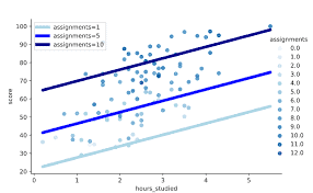
A sufficient summary plot (SSP) of the sufficient predictor $S P=\alpha+\boldsymbol{\beta}^T \boldsymbol{x}_i$ versus the response variable $Y_i$ with the mean function added as a visual aid can be useful for describing the multiple linear regression model. This plot can not be used for real data since $\alpha$ and $\boldsymbol{\beta}$ are unknown. To make Figure 1.1, the artificial data used $n=100$ cases with $k=5$ nontrivial predictors. The data used $\alpha=-1, \boldsymbol{\beta}=(1,2,3,0,0)^T, e_i \sim N(0,1)$ and $\boldsymbol{x}$ from a multivariate normal distribution $\boldsymbol{x} \sim N_5(\mathbf{0}, \boldsymbol{I})$.
In Figure 1.1, notice that the identity line with unit slope and zero intercept corresponds to the mean function since the identity line is the line $Y=S P=\alpha+\boldsymbol{\beta}^T \boldsymbol{x}=\mu(S P)=E(Y \mid S P)$. The vertical deviation of $Y_i$ from the line is equal to $e_i=Y_i-\left(\alpha+\boldsymbol{\beta}^T \boldsymbol{x}_i\right)$. For a given value of $S P$, $Y_i \sim N\left(S P, \sigma^2\right)$. For the artificial data, $\sigma^2=1$. Hence if $S P=0$ then $Y_i \sim N(0,1)$, and if $S P=5$ then $Y_i \sim N(5,1)$. Imagine superimposing the $N\left(S P, \sigma^2\right)$ curve at various values of $S P$. If all of the curves were shown, then the plot would resemble a road through a tunnel. For the artificial data, each $Y_i$ is a sample of size 1 from the normal curve with mean $\alpha+\boldsymbol{\beta}^T \boldsymbol{x}_i$.
线性回归代写
统计代写|线性回归分析代写linear regression analysis代考|Some Regression Models
在数据分析中,向调查人员提出问题和来自某些人群的数据。总体可能是实验所有可能结果的集合,而问 题可能是预测响应变量的末来值 $Y$ 或总结之间的关系 $Y$ 和 $p \times 1$ 预测变量向量 $\boldsymbol{x}$. 统计模型用于为生成数据 的人群的一些重要基本特征提供有用的近似值。下面定义的许多最常用的一维回归模型都是条件分布族 $Y \mid \boldsymbol{x}=\boldsymbol{x}o$ 被索引 $\boldsymbol{x}=\boldsymbol{x}_o$. 如果除了固定的有限数量的参数之外完全指定条件分布,则一维回归模型 是参数模型,否则, $1 \mathrm{D}$ 模型是一个半参数模型。下面定义的 GLM 和 GAM 将在第 13 章中介绍。 定义 1.1。回归研究响应变量如何 $Y$ 随 a 的值变化 $p \times 1$ 向量 $\boldsymbol{x}$ 的预测。通常这种条件分布 $Y \mid \boldsymbol{x}$ 被描述为 $1 D$ 回归模型,其中 $Y$ 有条件地独立于 $\boldsymbol{x}$ 给定足够的预测变量 $S P=h(\boldsymbol{x})$ ,写 $$ Y \backslash \operatorname{Perp} \boldsymbol{x} \mid S P \text { or } \mathrm{Y} \backslash \mathrm{Perp} \boldsymbol{x} \mid \mathrm{h}(\boldsymbol{x}) $$ 实值函数在哪里 $h: \mathbb{R}^p \rightarrow \mathbb{R}$. 估计足够的预测 $\mathrm{ESP}=\hat{h}(\boldsymbol{x})$. 一个重要的特例是具有线性预测器的模型 $h(\boldsymbol{x})=\alpha+\boldsymbol{\beta}^T \boldsymbol{x}$ 在哪里ESP $=\hat{\alpha}+\hat{\boldsymbol{\beta}}^T \boldsymbol{x}$. 此类模型包括广义线性模型 (GLM)。另一个重要的特例是广 义加法模型 (GAM),其中 $Y$ 独立于 $\boldsymbol{x}=\left(x_1, \ldots, x_p\right)^T$ 给定加法预测器 $A P=\alpha+\sum{j=1}^p S_j\left(x_j\right)$ 对 于某些 (通常是末知的) 功能 $S_j$. 估计的附加预测器 $\mathrm{EAP}=\mathrm{ESP}=\hat{\alpha}+\sum_{j=1}^p \hat{S}_j\left(x_j\right.$ ).
统计代写|线性回归分析代写linear regression analysis代考|Multiple Linear Regression
假设响应变量 $Y$ 是定量的,并且至少有一个预测变量 $x_i$ 是定量的。那么多元线性回归 (MLR) 模型往往是 一个非常有用的模型。对于 MLR 模型,
$$
Y_i=\alpha+x_{i, 1} \beta_1+x_{i, 2} \beta_2+\cdots+x_{i, p} \beta_p+e_i=\alpha+\boldsymbol{x}_i^T \boldsymbol{\beta}+e_i=\alpha+\boldsymbol{\beta}^T \boldsymbol{x}_i+e_i(1.9)
$$
为了 $i=1, \ldots, n$. 这里 $Y_i$ 是响应变量, $\boldsymbol{x}_i$ 是一个 $p \times 1$ 非平凡预测变量的向量, $\alpha$ 是末知常数, $\boldsymbol{\beta}$ 是一 个 $p \times 1$ 末知系数向量,和 $e_i$ 是一个称为误差的随机变量。
高斯或正态 MLR 模型额外假设误差 $e_i$ 是同龄人 $N\left(0, \sigma^2\right)$ 随机变量。这个模型也可以写成 $Y=\alpha+\boldsymbol{\beta}^T \boldsymbol{x}+e$ 在哪里 $e \sim N\left(0, \sigma^2\right)$ ,或者 $Y \mid \boldsymbol{x} \sim N\left(\alpha+\boldsymbol{\beta}^T \boldsymbol{x}, \sigma^2\right)$ ,或者 $Y \mid \boldsymbol{x} \sim$ $N\left(S P, \sigma^2\right)$ , 或者 $Y \mid S P \sim N\left(S P, \sigma^2\right)$. 正常的 MLR 模型是一个参数模型,因为给定 $\boldsymbol{x}$ ,条件分布 族完全由参数指定 $\alpha, \boldsymbol{\beta}$ ,和 $\sigma^2$. 自从 $Y \mid S P \sim N\left(S P, \sigma^2\right)$, 条件均值函数 $E(Y \mid S P) \equiv M(S P)=\mu(S P)=S P=\alpha+\boldsymbol{\beta}^T \boldsymbol{x}$. MLR 模型将在第 2、3 和 4 章中详细讨论。
充分预测变量的充分汇总图 (SSP) $S P=\alpha+\boldsymbol{\beta}^T \boldsymbol{x}_i$ 与响应变量 $Y_i$ 添加均值函数作为视觉辅助可用于描 述多元线性回归模型。该图不能用于真实数据,因为 $\alpha$ 和 $\beta$ 是末知的。为了制作图 1.1,使用了人工数据 $n=100$ 案件与 $k=5$ 非平凡的预测因子。使用的数据 $\alpha=-1, \boldsymbol{\beta}=(1,2,3,0,0)^T, e_i \sim N(0,1)$ 和 $\boldsymbol{x}$ 来自多元正态分布 $\boldsymbol{x} \sim N_5(\mathbf{0}, \boldsymbol{I})$.
在图 1.1 中,请注意具有单位斜率和零截距的恒等线对应于均值函数,因为恒等线是直线 $Y=S P=\alpha+\boldsymbol{\beta}^T \boldsymbol{x}=\mu(S P)=E(Y \mid S P)$. 的垂直偏差 $Y_i$ 从线等于 $e_i=Y_i-\left(\alpha+\boldsymbol{\beta}^T \boldsymbol{x}_i\right)$. 对于给定的值 $S P , Y_i \sim N\left(S P, \sigma^2\right)$. 对于人工数据, $\sigma^2=1$. 因此,如果 $S P=0$ 然后 $Y_i \sim N(0,1)$, 而如果 $S P=5$ 然后 $Y_i \sim N(5,1)$. 想象一下淔加 $N\left(S P, \sigma^2\right)$ 在各种值的曲线 $S P$. 如果显示所有曲线,则该图将类似于一条穿过隧道的道路。对于人工数据,每个 $Y_i$ 是来自均值为正态曲线 的大小为 1 的样本 $\alpha+\boldsymbol{\beta}^T \boldsymbol{x}_i$.

统计代写请认准statistics-lab™. statistics-lab™为您的留学生涯保驾护航。
随机过程代考
在概率论概念中,随机过程是随机变量的集合。 若一随机系统的样本点是随机函数,则称此函数为样本函数,这一随机系统全部样本函数的集合是一个随机过程。 实际应用中,样本函数的一般定义在时间域或者空间域。 随机过程的实例如股票和汇率的波动、语音信号、视频信号、体温的变化,随机运动如布朗运动、随机徘徊等等。
贝叶斯方法代考
贝叶斯统计概念及数据分析表示使用概率陈述回答有关未知参数的研究问题以及统计范式。后验分布包括关于参数的先验分布,和基于观测数据提供关于参数的信息似然模型。根据选择的先验分布和似然模型,后验分布可以解析或近似,例如,马尔科夫链蒙特卡罗 (MCMC) 方法之一。贝叶斯统计概念及数据分析使用后验分布来形成模型参数的各种摘要,包括点估计,如后验平均值、中位数、百分位数和称为可信区间的区间估计。此外,所有关于模型参数的统计检验都可以表示为基于估计后验分布的概率报表。
广义线性模型代考
广义线性模型(GLM)归属统计学领域,是一种应用灵活的线性回归模型。该模型允许因变量的偏差分布有除了正态分布之外的其它分布。
statistics-lab作为专业的留学生服务机构,多年来已为美国、英国、加拿大、澳洲等留学热门地的学生提供专业的学术服务,包括但不限于Essay代写,Assignment代写,Dissertation代写,Report代写,小组作业代写,Proposal代写,Paper代写,Presentation代写,计算机作业代写,论文修改和润色,网课代做,exam代考等等。写作范围涵盖高中,本科,研究生等海外留学全阶段,辐射金融,经济学,会计学,审计学,管理学等全球99%专业科目。写作团队既有专业英语母语作者,也有海外名校硕博留学生,每位写作老师都拥有过硬的语言能力,专业的学科背景和学术写作经验。我们承诺100%原创,100%专业,100%准时,100%满意。
机器学习代写
随着AI的大潮到来,Machine Learning逐渐成为一个新的学习热点。同时与传统CS相比,Machine Learning在其他领域也有着广泛的应用,因此这门学科成为不仅折磨CS专业同学的“小恶魔”,也是折磨生物、化学、统计等其他学科留学生的“大魔王”。学习Machine learning的一大绊脚石在于使用语言众多,跨学科范围广,所以学习起来尤其困难。但是不管你在学习Machine Learning时遇到任何难题,StudyGate专业导师团队都能为你轻松解决。
多元统计分析代考
基础数据: $N$ 个样本, $P$ 个变量数的单样本,组成的横列的数据表
变量定性: 分类和顺序;变量定量:数值
数学公式的角度分为: 因变量与自变量
时间序列分析代写
随机过程,是依赖于参数的一组随机变量的全体,参数通常是时间。 随机变量是随机现象的数量表现,其时间序列是一组按照时间发生先后顺序进行排列的数据点序列。通常一组时间序列的时间间隔为一恒定值(如1秒,5分钟,12小时,7天,1年),因此时间序列可以作为离散时间数据进行分析处理。研究时间序列数据的意义在于现实中,往往需要研究某个事物其随时间发展变化的规律。这就需要通过研究该事物过去发展的历史记录,以得到其自身发展的规律。
回归分析代写
多元回归分析渐进(Multiple Regression Analysis Asymptotics)属于计量经济学领域,主要是一种数学上的统计分析方法,可以分析复杂情况下各影响因素的数学关系,在自然科学、社会和经济学等多个领域内应用广泛。
MATLAB代写
MATLAB 是一种用于技术计算的高性能语言。它将计算、可视化和编程集成在一个易于使用的环境中,其中问题和解决方案以熟悉的数学符号表示。典型用途包括:数学和计算算法开发建模、仿真和原型制作数据分析、探索和可视化科学和工程图形应用程序开发,包括图形用户界面构建MATLAB 是一个交互式系统,其基本数据元素是一个不需要维度的数组。这使您可以解决许多技术计算问题,尤其是那些具有矩阵和向量公式的问题,而只需用 C 或 Fortran 等标量非交互式语言编写程序所需的时间的一小部分。MATLAB 名称代表矩阵实验室。MATLAB 最初的编写目的是提供对由 LINPACK 和 EISPACK 项目开发的矩阵软件的轻松访问,这两个项目共同代表了矩阵计算软件的最新技术。MATLAB 经过多年的发展,得到了许多用户的投入。在大学环境中,它是数学、工程和科学入门和高级课程的标准教学工具。在工业领域,MATLAB 是高效研究、开发和分析的首选工具。MATLAB 具有一系列称为工具箱的特定于应用程序的解决方案。对于大多数 MATLAB 用户来说非常重要,工具箱允许您学习和应用专业技术。工具箱是 MATLAB 函数(M 文件)的综合集合,可扩展 MATLAB 环境以解决特定类别的问题。可用工具箱的领域包括信号处理、控制系统、神经网络、模糊逻辑、小波、仿真等。