标签: STAT 6450

统计代写|回归分析作业代写Regression Analysis代考|Visualizing map patterns with eigenvectors

如果你也在 怎样代写回归分析Regression Analysis这个学科遇到相关的难题,请随时右上角联系我们的24/7代写客服。

回归分析是一种强大的统计方法,允许你检查两个或多个感兴趣的变量之间的关系。虽然有许多类型的回归分析,但它们的核心都是考察一个或多个自变量对因变量的影响。

statistics-lab™ 为您的留学生涯保驾护航 在代写回归分析Regression Analysis方面已经树立了自己的口碑, 保证靠谱, 高质且原创的统计Statistics代写服务。我们的专家在代写回归分析Regression Analysis代写方面经验极为丰富,各种代写回归分析Regression Analysis相关的作业也就用不着说。

我们提供的回归分析Regression Analysis及其相关学科的代写,服务范围广, 其中包括但不限于:

  • Statistical Inference 统计推断
  • Statistical Computing 统计计算
  • Advanced Probability Theory 高等楖率论
  • Advanced Mathematical Statistics 高等数理统计学
  • (Generalized) Linear Models 广义线性模型
  • Statistical Machine Learning 统计机器学习
  • Longitudinal Data Analysis 纵向数据分析
  • Foundations of Data Science 数据科学基础
统计代写|回归分析作业代写Regression Analysis代考|Visualizing map patterns with eigenvectors

统计代写|回归分析作业代写Regression Analysis代考|Visualizing map patterns with eigenvectors

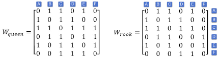
By convention, a SWM’s rows and columns are ordered with the same sequence of areal units. The eigenvectors of a SWM are n-by-1 vectors, with each of their rows linking to the corresponding areal unit identifier (ID) for the same row in their parent SWM. This one-to-one correspondence

enables mapping the eigenvectors of a SWM. The individual eigenvector elements simply have to be joined to their corresponding polygons in a shapefile file for visualization by ArcMap, for example.

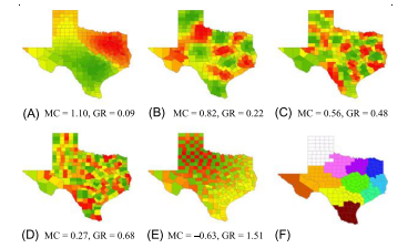
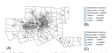
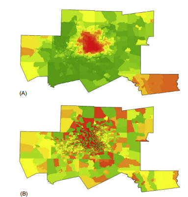
Fig. $2.4$ portrays the extreme eigenvectors for matrix $\left(I-11^{\mathrm{T}} / \mathrm{n}\right) \times$ $\mathbf{C}(\mathbf{I}-\mathbf{1 1} / \mathrm{n})$ representing the 2010 DFW metroplex census tracts. Fig. 2.4A portrays the principal eigenvector map pattern, the maximum PSA case, which depicts a hill/valley (this would change from a hill to a valley, or vice versa, by multiplying the eigenvector by $-1$ ) roughly in the center of the region, surrounded by a trough/hill, with intermediate plateaus in the western and southeastern parts of the region. This hill map pattern is one of the common global geographic trends portrayed by eigenvectors. Another typical map pattern is an east-west gradient trend, adapting to the somewhat rectangular shape of the DFW metroplex. Fig. $2.3 \mathrm{~A}$ reveals that the hill/valley subregion in Fig. 2.4A coincides with a concentration of numerous smaller census tracts located mostly in Dallas and Tarrant Counties. In contrast, Fig. 2.4B portrays a map pattern with considerable neighboring contrasts (e.g., dark red in juxtaposition with dark green), an alternating trend that exemplifies NSA. This map pattern has its intermediate values in its periphery, encircling the stark contrasts created by the alternating trend. A comparison of Fig. 2.4A and B reveals that PSA exhibits more smoothness in its map pattern, and NSA exhibits more fragmentation in its map pattern. These tendencies are less conspicuous in visualizations of the less extreme MC values.

统计代写|回归分析作业代写Regression Analysis代考|The spectral analysis of one-dimensional data

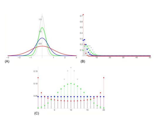
A simple one-dimensional geographic landscape (e.g., Fug. $2.5 \mathrm{~A}$ ) illustrates the connection between the spatial frequency and spatial spectral domains, furnishing the basis of the spectral density function equations presented in this section. SA indicates how rapidly a map pattern changes across a geographic landscape, using randomness as its yardstick. SA contains information about the expected frequency content mentioned earlier in this chapter. Meanwhile, the spectral density function furnishes one

mathematical link between $\mathrm{SA}$ and eigenfunctions in the spectral domain (Section 2.1; Bartlett, 1975). For a one-dimensional geographic landscape (e.g., Fig. $2.5 \mathrm{~A}$ ), given a stationary process $\left{\mathrm{X}{v}, \mathrm{t}=1,2, \ldots, \mathrm{T}\right}$ for a unidirectional dependency structure (this situation parallels a time series data structure) of the same form as the simultaneous autoregressive (SAR) model specification, $$ \mathrm{X}{\mathrm{t}}=\rho \mathrm{X}{\mathrm{t}-1}+\xi{\mathrm{t}},
$$
where $\rho$ is the autocorrelation parameter, $|\rho|<1$, t indexes location in the linear landscape, and $\xi_{t}$ is an independent and identically distributed (IID) random error term. Autocovariance functions, $\gamma(\tau), \tau=0,1, \ldots$, where $\tau$ denotes the number of lags, are established by repeatedly substituting the right-hand expression of an autoregressive equation like the preceding one into it and then applying the calculus of expectations to resulting infinite series forms of covariations. These infinite series are functions of linear combinations of $\xi_{t}^{2}$ together with powers of the SA parameter $\rho$, and hence yield $\sigma^{2}$ as well as a denominator term containing $\rho$. The corresponding atocovariance (i.e., covariation in an autocorrelated mathematical space) function is defined as follows:
$$
\gamma_{\mathrm{x}}(\tau)=\frac{\rho^{\tau} \sigma^{2}}{1-\rho^{2}}
$$
with $\tau$ being the number of lags (Griffith, 1988 , p- 111).
This preceding autocovariance function can be represented in the fretrency domain with the Fontrier transform
$$
f(\theta)=\frac{1}{2 \pi} \sum_{\tau=-\infty}^{\infty} e^{-i \pi \theta_{1}} \gamma_{X}(\tau)
$$

统计代写|回归分析作业代写Regression Analysis代考|This representation of the autocovariance

This representation of the autocovariance function in the frequency domain is referred to as the spectral density function or the spectrum of the random variable (RV) $\left{X_{t}\right}$. The sum ${ }^{6}$ of the spectrum over all frequencies gives the variance of $\left{X_{t}\right}$,
$$
\operatorname{VAR}\left(X_{t}\right)=\int_{0}^{\pi} \frac{\sigma^{2}}{2 \pi\left[1+\rho^{2}-2 \rho \operatorname{COS}(\theta)\right]} d \theta=\frac{\sigma^{2}}{2\left(1-\rho^{2}\right)},|\rho|<1,
$$
whereas the covariance at $\operatorname{lng} \tau$ is given by
$$
\operatorname{COV}\left(X_{t} X_{t-1}\right)=\int_{0}^{\pi} \frac{\sigma^{2} \operatorname{COS}(\tau \theta)}{2 \pi\left[1+\rho^{2}-2 \rho \operatorname{COS}(\theta)\right]} d \theta=\frac{\rho^{\tau} \sigma^{2}}{2\left(1-\rho^{2}\right)},|\rho|<1 .
$$
$\tau=0$ yields Eq. (2.6). In other words, representing the autocovariance function in the frequency domain allows a decomposition of the variance into frequency components that reveals their relative importance. The common effect of variance inflation routinely mentioned as a primary result of SA is apparent here: its arithmetic source is the term $-\rho^{2}$ appearing in the denominator of this expression. When no $S A$ is present, $\rho=0$ and $f(\theta)=\sigma^{2} / 2 \pi$, which is the spectral density for white noise. Accordingly, the variance in this independent observations case reduces to:

$$
\operatorname{VAR}\left(X_{\tau}\right)=\int_{0}^{\pi} \frac{\sigma^{2}}{2 \pi} \mathrm{d} \theta=\frac{\sigma^{2}}{2},
$$
which is consistent with results from the classical central limit theorem of statistics.

Furnishing asymptotic detaik for Eqs. (2.5) and (2.6), as shown by Berman and Plemmons (1994), the eigenvalues of a binary SWM for linear lattices can be defined as
$$
\lambda_{\mathrm{i}}=2 \operatorname{COS}\left(\frac{i \pi}{n+1}\right) .
$$
For the spectral density function defined by Eq. (2.5),
$$
\begin{gathered}
\lim {n \rightarrow \infty} \frac{i}{n+1}=\theta, \ \lambda{\mathrm{i}}=2 \operatorname{COS}(\theta), \text { and } \
f(\theta)=\frac{\sigma^{2}}{2 \pi\left(1+\rho^{2}-\rho \lambda\right)} .
\end{gathered}
$$
In other words, the spectral density function contains the eigenvalues of its corresponding SWM, which reveals that the autocovariance function for the RV $\left{X_{t}\right}$ is a function of the eigenvalues of the SWM.

To illustrate the relationship between the lagged spatial correlations with the second-order spatial covariance structure matrix $(\mathbf{I}-\rho \mathbf{C})^{-2}$ the SAR model specification-consider the bidirectional and one-dimensional geographic landscape with a symmetric dependency structure; that is,
$$
\mathrm{X}{\mathrm{i}}=\rho\left(\mathrm{X}{\mathrm{i}-1}+\mathrm{X}{\mathrm{i}+1}\right)+\xi{\mathrm{i}},|\rho|<\frac{1}{2}
$$
Here the autovariances at lags 0 and $\tau$ are
$$
\gamma(0)=\mathrm{E}\left(\mathrm{X}{\mathrm{i}} \mathrm{X}{\mathrm{i}}\right)=\frac{\sigma^{2}}{\left(1-4 \rho^{2}\right)^{3 / 2}}, \text { and }
$$
$\gamma(\tau)=\mathrm{E}\left(\mathrm{X}{\mathrm{i}} \mathrm{X}{\mathrm{i}-\tau}\right)$
$=\sigma^{2} \frac{\operatorname{SIN}[\tau \pi] \text { Hypergeometric PFQ }\left[\left{\frac{1}{2}, 1,2\right},{1-\tau, 1+\tau} 1-\tau, \frac{4 p}{1+2 p}\right]}{\pi \tau(1+2 p)^{2}}$ $0<\rho<1 / 2$

统计代写|回归分析作业代写Regression Analysis代考|Visualizing map patterns with eigenvectors

回归分析代写

统计代写|回归分析作业代写Regression Analysis代考|Visualizing map patterns with eigenvectors

按照惯例,SWM 的行和列按相同的面积单位顺序排列。SWM 的特征向量是 n×1 向量,它们的每一行都链接到其父 SWM 中同一行的相应区域单位标识符 (ID)。这种一一对应

能够映射 SWM 的特征向量。例如,为了通过 ArcMap 进行可视化,单个特征向量元素只需连接到 shapefile 文件中的相应多边形即可。

如图。2.4描绘矩阵的极端特征向量(一世−11吨/n)× C(一世−11/n)代表 2010 年 DFW 大都会人口普查区。图 2.4A 描绘了主要的特征向量图模式,即最大 PSA 情况,它描绘了一座山/谷(这会从一座山变为一座山谷,反之亦然,通过将特征向量乘以−1) 大致位于该地区的中心,被一个低谷/山丘包围,在该地区的西部和东南部有中间高原。这种山图模式是特征向量描绘的常见全球地理趋势之一。另一个典型的地图模式是东西向的渐变趋势,适应了 DFW 大都会的矩形形状。如图。2.3 一种揭示了图 2.4A 中的丘陵/山谷次区域与主要位于达拉斯和塔兰特县的众多较小人口普查区的集中相吻合。相比之下,图 2.4B 描绘了具有相当大的相邻对比度的地图图案(例如,深红色与深绿色并列),这是 NSA 的一种交替趋势。该地图模式在其外围具有中间值,围绕着由交替趋势产生的鲜明对比。图 2.4A 和 B 的比较表明,PSA 在其图谱中表现出更多的平滑度,而 NSA 在其图谱中表现出更多的碎片化。这些趋势在不太极端的 MC 值的可视化中不太明显。

统计代写|回归分析作业代写Regression Analysis代考|The spectral analysis of one-dimensional data

一个简单的一维地理景观(例如,Fug.2.5 一种) 说明了空间频率域和空间谱域之间的联系,为本节介绍的谱密度函数方程提供了基础。SA 表示地图模式在地理景观中的变化速度,使用随机性作为衡量标准。SA 包含有关本章前面提到的预期频率内容的信息。同时,谱密度函数提供了一个

之间的数学联系小号一种和谱域中的特征函数(第 2.1 节;Bartlett,1975)。对于一维地理景观(例如,图 1)。2.5 一种),给定一个平稳过程\left{\mathrm{X}{v}, \mathrm{t}=1,2, \ldots, \mathrm{T}\right}\left{\mathrm{X}{v}, \mathrm{t}=1,2, \ldots, \mathrm{T}\right}对于与同步自回归 (SAR) 模型规范相同形式的单向依赖结构(这种情况与时间序列数据结构平行),X吨=ρX吨−1+X吨,
在哪里ρ是自相关参数,|ρ|<1, t 索引线性景观中的位置,以及X吨是独立同分布 (IID) 随机误差项。自协方差函数,C(τ),τ=0,1,…, 在哪里τ表示滞后数,通过反复代入与前一个类似的自回归方程的右手表达式,然后将期望计算应用于所得的无限级数形式的协变来建立。这些无穷级数是线性组合的函数X吨2连同 SA 参数的幂ρ,因此产量σ2以及包含的分母项ρ. 相应的原子协方差(即自相关数学空间中的协变)函数定义如下:
CX(τ)=ρτσ21−ρ2
和τ是滞后的数量(Griffith,1988,p-111)。
前面的自协方差函数可以用 Fontrier 变换在频域中表示
F(θ)=12圆周率∑τ=−∞∞和−一世圆周率θ1CX(τ)

统计代写|回归分析作业代写Regression Analysis代考|This representation of the autocovariance

这种自协方差函数在频域中的表示称为谱密度函数或随机变量 (RV) 的谱\left{X_{t}\right}\left{X_{t}\right}. 总和6在所有频率上的频谱给出方差\left{X_{t}\right}\left{X_{t}\right},
曾是⁡(X吨)=∫0圆周率σ22圆周率[1+ρ2−2ρCOS⁡(θ)]dθ=σ22(1−ρ2),|ρ|<1,
而协方差在液化天然气⁡τ是(谁)给的
冠状病毒⁡(X吨X吨−1)=∫0圆周率σ2COS⁡(τθ)2圆周率[1+ρ2−2ρCOS⁡(θ)]dθ=ρτσ22(1−ρ2),|ρ|<1.
τ=0产生方程。(2.6)。换句话说,在频域中表示自协方差函数允许将方差分解为频率分量,从而揭示它们的相对重要性。作为 SA 的主要结果,经常提到的方差膨胀的共同影响在这里很明显:它的算术来源是术语−ρ2出现在这个表达式的分母中。没有时小号一种存在,ρ=0和F(θ)=σ2/2圆周率,这是白噪声的频谱密度。因此,这种独立观察情况下的方差减少到:曾是⁡(Xτ)=∫0圆周率σ22圆周率dθ=σ22,
这与统计的经典中心极限定理的结果一致。

为 Eqs 提供渐近细节。(2.5) 和 (2.6),如 Berman 和 Plemmons (1994) 所示,线性格的二进制 SWM 的特征值可以定义为
λ一世=2COS⁡(一世圆周率n+1).
对于方程定义的谱密度函数。(2.5),
$$
\begin{gathered}
\lim {n \rightarrow \infty} \frac{i}{n+1}=\theta, \ \lambda {\mathrm{i}}=2 \operatorname{COS }(\theta), \text { 和 } \
f(\theta)=\frac{\sigma^{2}}{2 \pi\left(1+\rho^{2}-\rho \lambda\right )} 。
\end{gathered}
$$
换句话说,谱密度函数包含其对应 SWM 的特征值,这表明 RV 的自协方差函数\left{X_{t}\right}\left{X_{t}\right}是 SWM 特征值的函数。

为了说明滞后空间相关性与二阶空间协方差结构矩阵之间的关系(一世−ρC)−2SAR模型规范——考虑具有对称依赖结构的双向一维地理景观;那是,
X一世=ρ(X一世−1+X一世+1)+X一世,|ρ|<12
这里的自方差滞后 0 和τ是
C(0)=和(X一世X一世)=σ2(1−4ρ2)3/2, 和 
C(τ)=和(X一世X一世−τ)
=\sigma^{2} \frac{\operatorname{SIN}[\tau \pi] \text { 超几何 PFQ }\left[\left{\frac{1}{2}, 1,2\right},{ 1-\tau, 1+\tau} 1-\tau, \frac{4 p}{1+2 p}\right]}{\pi \tau(1+2 p)^{2}}=\sigma^{2} \frac{\operatorname{SIN}[\tau \pi] \text { 超几何 PFQ }\left[\left{\frac{1}{2}, 1,2\right},{ 1-\tau, 1+\tau} 1-\tau, \frac{4 p}{1+2 p}\right]}{\pi \tau(1+2 p)^{2}} 0<ρ<1/2

统计代写|回归分析作业代写Regression Analysis代考 请认准statistics-lab™

统计代写请认准statistics-lab™. statistics-lab™为您的留学生涯保驾护航。

随机过程代考

在概率论概念中,随机过程随机变量的集合。 若一随机系统的样本点是随机函数,则称此函数为样本函数,这一随机系统全部样本函数的集合是一个随机过程。 实际应用中,样本函数的一般定义在时间域或者空间域。 随机过程的实例如股票和汇率的波动、语音信号、视频信号、体温的变化,随机运动如布朗运动、随机徘徊等等。

贝叶斯方法代考

贝叶斯统计概念及数据分析表示使用概率陈述回答有关未知参数的研究问题以及统计范式。后验分布包括关于参数的先验分布,和基于观测数据提供关于参数的信息似然模型。根据选择的先验分布和似然模型,后验分布可以解析或近似,例如,马尔科夫链蒙特卡罗 (MCMC) 方法之一。贝叶斯统计概念及数据分析使用后验分布来形成模型参数的各种摘要,包括点估计,如后验平均值、中位数、百分位数和称为可信区间的区间估计。此外,所有关于模型参数的统计检验都可以表示为基于估计后验分布的概率报表。

广义线性模型代考

广义线性模型(GLM)归属统计学领域,是一种应用灵活的线性回归模型。该模型允许因变量的偏差分布有除了正态分布之外的其它分布。

statistics-lab作为专业的留学生服务机构,多年来已为美国、英国、加拿大、澳洲等留学热门地的学生提供专业的学术服务,包括但不限于Essay代写,Assignment代写,Dissertation代写,Report代写,小组作业代写,Proposal代写,Paper代写,Presentation代写,计算机作业代写,论文修改和润色,网课代做,exam代考等等。写作范围涵盖高中,本科,研究生等海外留学全阶段,辐射金融,经济学,会计学,审计学,管理学等全球99%专业科目。写作团队既有专业英语母语作者,也有海外名校硕博留学生,每位写作老师都拥有过硬的语言能力,专业的学科背景和学术写作经验。我们承诺100%原创,100%专业,100%准时,100%满意。

机器学习代写

随着AI的大潮到来,Machine Learning逐渐成为一个新的学习热点。同时与传统CS相比,Machine Learning在其他领域也有着广泛的应用,因此这门学科成为不仅折磨CS专业同学的“小恶魔”,也是折磨生物、化学、统计等其他学科留学生的“大魔王”。学习Machine learning的一大绊脚石在于使用语言众多,跨学科范围广,所以学习起来尤其困难。但是不管你在学习Machine Learning时遇到任何难题,StudyGate专业导师团队都能为你轻松解决。

多元统计分析代考


基础数据: $N$ 个样本, $P$ 个变量数的单样本,组成的横列的数据表
变量定性: 分类和顺序;变量定量:数值
数学公式的角度分为: 因变量与自变量

时间序列分析代写

随机过程,是依赖于参数的一组随机变量的全体,参数通常是时间。 随机变量是随机现象的数量表现,其时间序列是一组按照时间发生先后顺序进行排列的数据点序列。通常一组时间序列的时间间隔为一恒定值(如1秒,5分钟,12小时,7天,1年),因此时间序列可以作为离散时间数据进行分析处理。研究时间序列数据的意义在于现实中,往往需要研究某个事物其随时间发展变化的规律。这就需要通过研究该事物过去发展的历史记录,以得到其自身发展的规律。

回归分析代写

多元回归分析渐进(Multiple Regression Analysis Asymptotics)属于计量经济学领域,主要是一种数学上的统计分析方法,可以分析复杂情况下各影响因素的数学关系,在自然科学、社会和经济学等多个领域内应用广泛。

MATLAB代写

MATLAB 是一种用于技术计算的高性能语言。它将计算、可视化和编程集成在一个易于使用的环境中,其中问题和解决方案以熟悉的数学符号表示。典型用途包括:数学和计算算法开发建模、仿真和原型制作数据分析、探索和可视化科学和工程图形应用程序开发,包括图形用户界面构建MATLAB 是一个交互式系统,其基本数据元素是一个不需要维度的数组。这使您可以解决许多技术计算问题,尤其是那些具有矩阵和向量公式的问题,而只需用 C 或 Fortran 等标量非交互式语言编写程序所需的时间的一小部分。MATLAB 名称代表矩阵实验室。MATLAB 最初的编写目的是提供对由 LINPACK 和 EISPACK 项目开发的矩阵软件的轻松访问,这两个项目共同代表了矩阵计算软件的最新技术。MATLAB 经过多年的发展,得到了许多用户的投入。在大学环境中,它是数学、工程和科学入门和高级课程的标准教学工具。在工业领域,MATLAB 是高效研究、开发和分析的首选工具。MATLAB 具有一系列称为工具箱的特定于应用程序的解决方案。对于大多数 MATLAB 用户来说非常重要,工具箱允许您学习应用专业技术。工具箱是 MATLAB 函数(M 文件)的综合集合,可扩展 MATLAB 环境以解决特定类别的问题。可用工具箱的领域包括信号处理、控制系统、神经网络、模糊逻辑、小波、仿真等。

R语言代写问卷设计与分析代写
PYTHON代写回归分析与线性模型代写
MATLAB代写方差分析与试验设计代写
STATA代写机器学习/统计学习代写
SPSS代写计量经济学代写
EVIEWS代写时间序列分析代写
EXCEL代写深度学习代写
SQL代写各种数据建模与可视化代写

统计代写|回归分析作业代写Regression Analysis代考|Principal components analysis: A reconnaissance

如果你也在 怎样代写回归分析Regression Analysis这个学科遇到相关的难题,请随时右上角联系我们的24/7代写客服。

回归分析是一种强大的统计方法,允许你检查两个或多个感兴趣的变量之间的关系。虽然有许多类型的回归分析,但它们的核心都是考察一个或多个自变量对因变量的影响。

statistics-lab™ 为您的留学生涯保驾护航 在代写回归分析Regression Analysis方面已经树立了自己的口碑, 保证靠谱, 高质且原创的统计Statistics代写服务。我们的专家在代写回归分析Regression Analysis代写方面经验极为丰富,各种代写回归分析Regression Analysis相关的作业也就用不着说。

我们提供的回归分析Regression Analysis及其相关学科的代写,服务范围广, 其中包括但不限于:

  • Statistical Inference 统计推断
  • Statistical Computing 统计计算
  • Advanced Probability Theory 高等楖率论
  • Advanced Mathematical Statistics 高等数理统计学
  • (Generalized) Linear Models 广义线性模型
  • Statistical Machine Learning 统计机器学习
  • Longitudinal Data Analysis 纵向数据分析
  • Foundations of Data Science 数据科学基础
统计代写|回归分析作业代写Regression Analysis代考|Principal components analysis: A reconnaissance

统计代写|回归分析作业代写Regression Analysis代考|Principal components analysis: A reconnaissance

Eigendecomposition (i.e., rewriting a matrix in terms of its eigenvalues and eigenvectors) of a correlation matrix produces a set of eigenvalues that can be arranged in descending order, along with their corresponding eigenvectors. These eigenvectors are referred to as principals components (PCs) and have the intriguing property that the amount of variance they capture follows the same order as their magnitudes. In other words, the first eigenvector sum$\mathrm{~ m a n i z e s ~ t h e ~ m u s l ~ v a n i a n e , ~ t h e ~ s e c o n d ~ c i g c u v e l t e n ~ s u m u a r e s s ~ t h e ~ s e c u a}$ largest amount of varianec, and so forth. Because the first few cigenvectors often are sufficient for representing most of the information contained in their correlation matrix, principal components analysis (PCA) commonly is used for variable selection. However, here we use PCA to illustrate linkages between eigenvectors and SA.

Griffith (1984) began to explore the application of PCA to the binary SWM C, initially making little headway because the analysis was of $n$ indicator variable correlation (i.e., phi) coefficients. Later, a simple modification of matrix $\mathbf{C}$ illuminated a breakthrough: adding an identity matrix to $\mathbf{C}$ [i.e., $(\mathbf{C}+\mathbf{I})$ ] renders a SWM mimicking a correlation matrix, allowing the application of conventional PCA to it in a way that yields interpretable results (see Appendix 2.A). Furthermore, based on the mathematical properties of eigenvalues and eigenvectors, matrices $(\mathbf{C}+\mathbf{I})$ and $\mathbf{C}$ have the same eigenvectors and the same eigenvalues if one is added to the eigenvalues of matrix $\mathrm{C}$ (i.e., $\lambda_{j}+1$ ). The resulting PCA gives an important insight into the asymptotic relationship between the $\mathrm{SWM} \mathrm{C}$ eigenvectors and $\mathrm{SA}$ : the second $\mathrm{PC}$ corresponds to the maximum positive SA (PSA), and the last $\mathrm{PC}$ to the maximum negative SA (NSA). More specifically, PCA made possible the discovery of, and now makes obvious, the fundamental theorem of MESF, which pertains to matrix $\left(\mathrm{I}-11^{\mathrm{T}} / \mathrm{n}\right) \mathbf{C}\left(\mathbf{I}-11^{\mathrm{T}} / \mathrm{n}\right)$ .

统计代写|回归分析作业代写Regression Analysis代考|The spectral decomposition of a modified SWM

The MC can be written in matrix form as
The modified matrix $\left(\mathbf{I}-11^{\mathrm{T}} / \mathrm{n}\right) \mathrm{C}\left(\mathrm{I}-11^{\mathrm{T}} / \mathrm{n}\right)$ in its numerator is the matrix that relates to SA. Accordingly, the pair of eigenfunction problems becomes
$$
\operatorname{Det}\left[\left(\mathbf{I}-11^{\mathrm{T}} / \mathrm{n}\right) \mathbf{C}\left(\mathbf{I}-11^{\mathrm{T}} / \mathrm{n}\right)-\lambda \mathbf{I}\right]=0
$$
and
$$
\left[\left(\mathbf{I}-11^{\mathrm{T}} / \mathrm{n}\right) \mathbf{C}\left(\mathbf{I}-11^{\mathrm{T}} / \mathrm{n}\right)-\lambda_{\mathrm{j}} \mathbf{I}\right] \mathbf{E}_{\mathrm{j}}=0, \mathrm{j}=1,2, \ldots, \mathrm{n}
$$

subject to $\mathbf{E}{j}^{\mathrm{T}} \mathbf{E}{j}=1$ and $\mathbf{E}{j}^{\mathrm{T}} \mathbf{E}{\mathrm{k}}=0, j \neq k$. Because matrix $\left(\mathbf{I}-11^{\mathrm{T}} / \mathrm{n}\right) \times$ $\mathbf{C}\left(\mathbf{I}-11^{\mathrm{T}} / \mathrm{n}\right)$ is square and symmetric, it can be decomposed into a series of rank 1 matrices consisting of the products of the eigenvalues and eigenvectors; that is,
$$
\left(\mathbf{I}-\frac{11^{\mathrm{T}}}{n}\right) \mathbf{C}\left(\mathbf{I}-\frac{11^{\mathrm{T}}}{n}\right)=\sum_{j=1}^{n} \lambda_{j} \mathbf{E}{j} \mathbf{E}{j}^{\mathrm{T}}
$$
This right-hand summation expression is a matrix expansion of the standard eigendecomposition $\left(\mathbf{I}-11^{\mathrm{T}} / \mathrm{n}\right) \mathbf{C}\left(\mathbf{I}-11^{\mathrm{T}} / \mathrm{n}\right)=\mathbf{E} \Lambda \mathbf{E}^{\mathrm{T}}$, where $\Lambda$ is the diagonal matrix containing the n eigenvalues $\lambda_{\mathrm{j}}$

统计代写|回归分析作业代写Regression Analysis代考|Representing the MC with eigenfunctions

Let vector $\mathbf{Y}=\mathbf{E}{j}$. Next, substitute $\mathbf{E}{j}$ into Eq. (2.4):
$$
\begin{gathered}
{\left[\mathrm{n} /\left(\mathbf{1}^{\mathrm{T}} \mathbf{C} 1\right)\right] \mathbf{E}{\mathrm{j}}^{\mathrm{T}}\left(\mathbf{I}-11^{\mathrm{T}} / \mathrm{n}\right) \mathbf{C}(\mathbf{I}-\mathbf{1 1} / \mathrm{T}) \mathbf{E}{\mathrm{j}} /} \
{\left[\mathbf{E}{\mathrm{j}}^{\mathrm{T}}\left(\mathbf{I}-\mathbf{1 1} \mathbf{T}^{\mathrm{T}} / \mathrm{n}\right) \mathbf{E}{\mathrm{j}}\right]=\left[\mathrm{n} /\left(\mathbf{1}^{\mathrm{T}} \mathbf{C} 1\right)\right] \lambda_{\mathrm{j}} / 1}
\end{gathered}
$$
which is the same as Eq. (2.3). This outcome highlights why the extreme eigenvalues of matrix $\left(\mathrm{I}-11^{\mathrm{T}} / \mathrm{n}\right) \mathbf{C}\left(\mathbf{I}-11^{\mathrm{T}} / \mathrm{n}\right), \lambda_{1}$ and $\lambda_{\mathrm{m}}$, respectively, define the maximum and minimum values of a $\mathrm{MC}$ – they optimize its Rayleigh quotient. This feature of the MC distinguishes it from a Pearson product moment correlation coefficient: it does not have extreme values of $\pm 1$ but rather has an upper bound that often exceeds 1 by as much as $0.15$, or more, and a lower bound that often is closer to $-0.5$ than to $-1$.

Fig. 2.3A portrays the 2010 census tract surface partitioning $(n=1052)$ for the Dallas-Fort Worth (DFW) metroplex, and Fig. 2.3B is ArcMap SA output. The principal eigenvalue for this surface partitioning is $6.2675604$, based on the rook’s contiguity, with $1^{\mathrm{T}} \mathbf{C} 1=5626$. Therefore for PSA, $\mathrm{MC}=(1052 / 5626)(6.2675604)=1.171965$. This maximum PSA value exceeds 1 by $>0.17$. Meanwhile, for $\mathrm{NSA}, \quad \mathrm{MC}=(1052 / 5626) \times$ $(-3.949034)=-0.738426$. This maximum NSA value is closer to $-0.5$ than to $-1$.

统计代写|回归分析作业代写Regression Analysis代考|Principal components analysis: A reconnaissance

回归分析代写

统计代写|回归分析作业代写Regression Analysis代考|Principal components analysis: A reconnaissance

相关矩阵的特征分解(即,根据其特征值和特征向量重写矩阵)产生一组可以按降序排列的特征值及其对应的特征向量。这些特征向量被称为主成分 (PC),并且具有一个有趣的特性,即它们捕获的方差量与其大小遵循相同的顺序。换句话说,第一个特征向量和 米一种n一世和和s 吨H和 米在sl 在一种n一世一种n和, 吨H和 s和C这nd C一世GC在在和l吨和n s在米在一种r和ss 吨H和 s和C在一种最大量的 varianec,依此类推。由于前几个特征向量通常足以表示其相关矩阵中包含的大部分信息,因此主成分分析(PCA)通常用于变量选择。然而,这里我们使用 PCA 来说明特征向量和 SA 之间的联系。

Griffith (1984) 开始探索将 PCA 应用于二进制 SWM C,最初进展不大,因为分析是n指标变量相关(即phi)系数。后来对矩阵进行了简单的修改C阐明了一个突破:将单位矩阵添加到C[IE,(C+一世)] 呈现模拟相关矩阵的 SWM,允许以产生可解释结果的方式将常规 PCA 应用于它(参见附录 2.A)。此外,基于特征值和特征向量的数学性质,矩阵(C+一世)和C如果将一个添加到矩阵的特征值中,则具有相同的特征向量和相同的特征值C(IE,λj+1)。由此产生的 PCA 提供了一个重要的洞察力之间的渐近关系小号在米C特征向量和小号一种: 第二磷C对应于最大正 SA (PSA),最后一个磷C到最大负 SA (NSA)。更具体地说,PCA 使MESF 基本定理的发现成为可能,并且现在使之变得显而易见,该定理与矩阵有关(一世−11吨/n)C(一世−11吨/n) .

统计代写|回归分析作业代写Regression Analysis代考|The spectral decomposition of a modified SWM

MC 可以写成矩阵形式为
修改后的矩阵(一世−11吨/n)C(一世−11吨/n)在其分子中是与 SA 相关的矩阵。因此,这对特征函数问题变为
这⁡[(一世−11吨/n)C(一世−11吨/n)−λ一世]=0

[(一世−11吨/n)C(一世−11吨/n)−λj一世]和j=0,j=1,2,…,n

服从 \ \ mathbf {E} {j} ^ {mathrm {T}} th mathbf {E} {j}一种nd\ mathbf {E} {j} ^ {th mathrm {T}} \ mathbf {E} {th mathrm {k}} = 0, j \neq k.乙和C一种在s和米一种吨r一世X\left(\mathbf{I}-11^{\mathrm{T}} / \mathrm{n}\right) \times\mathbf{C}\left(\mathbf{I}-11^{\mathrm{T}} / \mathrm{n}\right)一世ssq在一种r和一种nds是米米和吨r一世C,一世吨C一种nb和d和C这米p这s和d一世n吨这一种s和r一世和s这Fr一种nķ1米一种吨r一世C和sC这ns一世s吨一世nG这F吨H和pr这d在C吨s这F吨H和和一世G和n在一种l在和s一种nd和一世G和n在和C吨这rs;吨H一种吨一世s,$
\left(\mathbf{I}-\frac{11^{\mathrm{T}}}{n}\right) \mathbf{C}\left(\mathbf{I}-\frac{11^{\ mathrm{T}}}{n}\right)=\sum_{j=1}^{n} \lambda_{j} \mathbf{E} {j} \mathbf{E} {j}^{\mathrm{ T}}
$$
这个右手求和表达式是标准特征分解的矩阵展开(一世−11吨/n)C(一世−11吨/n)=和Λ和吨, 在哪里Λ是包含 n 个特征值的对角矩阵λj

统计代写|回归分析作业代写Regression Analysis代考|Representing the MC with eigenfunctions

让向量是=和j. 接下来,替换和j进入方程。(2.4):
[n/(1吨C1)]和j吨(一世−11吨/n)C(一世−11/吨)和j/ [和j吨(一世−11吨吨/n)和j]=[n/(1吨C1)]λj/1
这与等式相同。(2.3)。这个结果突出了为什么矩阵的极端特征值(一世−11吨/n)C(一世−11吨/n),λ1和λ米,分别定义a的最大值和最小值米C– 他们优化了瑞利商。MC 的这一特征将其与 Pearson 乘积矩相关系数区分开来:它没有极值±1而是有一个经常超过 1 的上限0.15,或更多,以及通常更接近的下限−0.5比−1.

图 2.3A 描绘了 2010 年人口普查区域的表面划分(n=1052)对于达拉斯-沃思堡 (DFW) 大都市,图 2.3B 是 ArcMap SA 输出。这种表面划分的主要特征值为6.2675604,基于车的邻接性,与1吨C1=5626. 因此对于 PSA,米C=(1052/5626)(6.2675604)=1.171965. 此最大 PSA 值超过 1>0.17. 同时,对于ñ小号一种,米C=(1052/5626)× (−3.949034)=−0.738426. 这个最大的 NSA 值更接近−0.5比−1.

统计代写|回归分析作业代写Regression Analysis代考 请认准statistics-lab™

统计代写请认准statistics-lab™. statistics-lab™为您的留学生涯保驾护航。

随机过程代考

在概率论概念中,随机过程随机变量的集合。 若一随机系统的样本点是随机函数,则称此函数为样本函数,这一随机系统全部样本函数的集合是一个随机过程。 实际应用中,样本函数的一般定义在时间域或者空间域。 随机过程的实例如股票和汇率的波动、语音信号、视频信号、体温的变化,随机运动如布朗运动、随机徘徊等等。

贝叶斯方法代考

贝叶斯统计概念及数据分析表示使用概率陈述回答有关未知参数的研究问题以及统计范式。后验分布包括关于参数的先验分布,和基于观测数据提供关于参数的信息似然模型。根据选择的先验分布和似然模型,后验分布可以解析或近似,例如,马尔科夫链蒙特卡罗 (MCMC) 方法之一。贝叶斯统计概念及数据分析使用后验分布来形成模型参数的各种摘要,包括点估计,如后验平均值、中位数、百分位数和称为可信区间的区间估计。此外,所有关于模型参数的统计检验都可以表示为基于估计后验分布的概率报表。

广义线性模型代考

广义线性模型(GLM)归属统计学领域,是一种应用灵活的线性回归模型。该模型允许因变量的偏差分布有除了正态分布之外的其它分布。

statistics-lab作为专业的留学生服务机构,多年来已为美国、英国、加拿大、澳洲等留学热门地的学生提供专业的学术服务,包括但不限于Essay代写,Assignment代写,Dissertation代写,Report代写,小组作业代写,Proposal代写,Paper代写,Presentation代写,计算机作业代写,论文修改和润色,网课代做,exam代考等等。写作范围涵盖高中,本科,研究生等海外留学全阶段,辐射金融,经济学,会计学,审计学,管理学等全球99%专业科目。写作团队既有专业英语母语作者,也有海外名校硕博留学生,每位写作老师都拥有过硬的语言能力,专业的学科背景和学术写作经验。我们承诺100%原创,100%专业,100%准时,100%满意。

机器学习代写

随着AI的大潮到来,Machine Learning逐渐成为一个新的学习热点。同时与传统CS相比,Machine Learning在其他领域也有着广泛的应用,因此这门学科成为不仅折磨CS专业同学的“小恶魔”,也是折磨生物、化学、统计等其他学科留学生的“大魔王”。学习Machine learning的一大绊脚石在于使用语言众多,跨学科范围广,所以学习起来尤其困难。但是不管你在学习Machine Learning时遇到任何难题,StudyGate专业导师团队都能为你轻松解决。

多元统计分析代考


基础数据: $N$ 个样本, $P$ 个变量数的单样本,组成的横列的数据表
变量定性: 分类和顺序;变量定量:数值
数学公式的角度分为: 因变量与自变量

时间序列分析代写

随机过程,是依赖于参数的一组随机变量的全体,参数通常是时间。 随机变量是随机现象的数量表现,其时间序列是一组按照时间发生先后顺序进行排列的数据点序列。通常一组时间序列的时间间隔为一恒定值(如1秒,5分钟,12小时,7天,1年),因此时间序列可以作为离散时间数据进行分析处理。研究时间序列数据的意义在于现实中,往往需要研究某个事物其随时间发展变化的规律。这就需要通过研究该事物过去发展的历史记录,以得到其自身发展的规律。

回归分析代写

多元回归分析渐进(Multiple Regression Analysis Asymptotics)属于计量经济学领域,主要是一种数学上的统计分析方法,可以分析复杂情况下各影响因素的数学关系,在自然科学、社会和经济学等多个领域内应用广泛。

MATLAB代写

MATLAB 是一种用于技术计算的高性能语言。它将计算、可视化和编程集成在一个易于使用的环境中,其中问题和解决方案以熟悉的数学符号表示。典型用途包括:数学和计算算法开发建模、仿真和原型制作数据分析、探索和可视化科学和工程图形应用程序开发,包括图形用户界面构建MATLAB 是一个交互式系统,其基本数据元素是一个不需要维度的数组。这使您可以解决许多技术计算问题,尤其是那些具有矩阵和向量公式的问题,而只需用 C 或 Fortran 等标量非交互式语言编写程序所需的时间的一小部分。MATLAB 名称代表矩阵实验室。MATLAB 最初的编写目的是提供对由 LINPACK 和 EISPACK 项目开发的矩阵软件的轻松访问,这两个项目共同代表了矩阵计算软件的最新技术。MATLAB 经过多年的发展,得到了许多用户的投入。在大学环境中,它是数学、工程和科学入门和高级课程的标准教学工具。在工业领域,MATLAB 是高效研究、开发和分析的首选工具。MATLAB 具有一系列称为工具箱的特定于应用程序的解决方案。对于大多数 MATLAB 用户来说非常重要,工具箱允许您学习应用专业技术。工具箱是 MATLAB 函数(M 文件)的综合集合,可扩展 MATLAB 环境以解决特定类别的问题。可用工具箱的领域包括信号处理、控制系统、神经网络、模糊逻辑、小波、仿真等。

R语言代写问卷设计与分析代写
PYTHON代写回归分析与线性模型代写
MATLAB代写方差分析与试验设计代写
STATA代写机器学习/统计学习代写
SPSS代写计量经济学代写
EVIEWS代写时间序列分析代写
EXCEL代写深度学习代写
SQL代写各种数据建模与可视化代写

统计代写|回归分析作业代写Regression Analysis代考|An introduction to spectral

如果你也在 怎样代写回归分析Regression Analysis这个学科遇到相关的难题,请随时右上角联系我们的24/7代写客服。

回归分析是一种强大的统计方法,允许你检查两个或多个感兴趣的变量之间的关系。虽然有许多类型的回归分析,但它们的核心都是考察一个或多个自变量对因变量的影响。

statistics-lab™ 为您的留学生涯保驾护航 在代写回归分析Regression Analysis方面已经树立了自己的口碑, 保证靠谱, 高质且原创的统计Statistics代写服务。我们的专家在代写回归分析Regression Analysis代写方面经验极为丰富,各种代写回归分析Regression Analysis相关的作业也就用不着说。

我们提供的回归分析Regression Analysis及其相关学科的代写,服务范围广, 其中包括但不限于:

  • Statistical Inference 统计推断
  • Statistical Computing 统计计算
  • Advanced Probability Theory 高等楖率论
  • Advanced Mathematical Statistics 高等数理统计学
  • (Generalized) Linear Models 广义线性模型
  • Statistical Machine Learning 统计机器学习
  • Longitudinal Data Analysis 纵向数据分析
  • Foundations of Data Science 数据科学基础
统计代写|回归分析作业代写Regression Analysis代考|An introduction to spectral

统计代写|回归分析作业代写Regression Analysis代考|Representing SA in the spectral domain

A close relationship exists between SA and the spectral domain (see Bartlett, 1975). A spatial domain refers to how a map pattern changes over space, with this geographic variation relating to SA, whereas a spectral domain refers to how much of the map pattern lies within each given frequency band over a range of frequencies, which constitutes a spectrum. A mathematical function relates these two domains.

Tiefelsdorf and Boots $(1995)$ establish an important link between a n-by-n SWM C and SA: the eigenvalues of a modified SWM, namely, the Moran coefficient $(\mathrm{MC})$ numerator matrix expression $\left(\mathrm{I}-11^{\mathrm{T}} / \mathrm{n}\right) \times$ $\mathbf{C}\left(\mathbf{I}-11^{\mathrm{T}} / \mathrm{n}\right)$ involving pre- and postmultiplication of a $\mathrm{SWM}$ by a standard projection matrix, ${ }^{3}$ index all possible distinct natures and degrees of $\mathrm{SA}$ associated with a given SWM. This set of eigenvalues constitutes a spectrum. Griffith (1996) establishes the accompanying link between SA and map pattern: a linear combination of the eigenvectors of the aforementioned modified SWM describes the map pattern exhibited by a geographic distribution.

统计代写|回归分析作业代写Regression Analysis代考|From a spatial frequency to a spatial spectral domain

Table $2.1$ and Fig. $2.1$ present a common interface between spatial analysts and spectral concepts, namely, a remotely sensed satellite image. Here a multisensor instrument records wavelength measurements of electromagnetic radiation, with each discrete, distinctly recorded wavelength interval measured by a sensor constituting a band. In this context, the term spectrum refers to classifying a measurement according to its position on a scale between two extreme or opposite points. This general definition acknowledges that many types of measurements can be labeled spectra. Those of interest in this chapter include SWM eigenvalues and spatial correlations. A glass prism 4 exemplifies the notion of a spectrum specifically with regard to remotely sensed images (Fig. $2.2 \mathrm{~A}$ ).

The notion of a spectrum implies two distinct reference points for spatial statistical analysis. One is known as the frequency domain, and the other is known as the spectral domain. A spatial frequency domain refers to the frequency with which map attribute values change over a geographic landscape. This is the domain in which MESF operates. It relates to spatial autoregression and hence to inverse spatial covariance matrices constructed with SWMs. The other – the spectral domain – deals with spatial correlation and furnishes selected geographic landscape equations (i.e., spectral density functions) for calculating these correlations. This is the domain in which geostatistics operates. It relates to semivariogram models and hence to spatial covariance matrices (rather than their inverses). SWMs, among other mathematical tools, bridge these two domains (with the matrix inversion operation difference between them magnifying geographic edge effects between these two forms of spatial statistical analysis). This chapter highlights MESF eigenvalues that appear in spectral density functions, emphasizing this linkage.

统计代写|回归分析作业代写Regression Analysis代考|Eigenvalues and eigenvectors

Multivariate statistical analysis is perhaps the most common subject area in which researchers and students alike first encounter eigenfunctions. In this setting, calculations of these mathematical quantities are for correlation and covariance matrices, among others, and they relate to patterns of multicollinearity. Consequently, that eigenfunctions for SWMs are useful and illuminating should not be a surprise.

Regardless of whether a correlation matrix, a SWM, or some other square matrix is of interest, calculation of eigenfunctions remains the same. Eigenvalues for a given real $n$-by-n matrix $C$ are the $n$ roots of the polynomial defined by.
$$
\operatorname{Det}(\mathbf{C}-\lambda \mathbf{I})=0,
$$
where Det denotes the matrix determinant operation, and $\lambda$ denotes an eigenvalue. The solution to this $n$ th-order polynomial is the set of $n$ eigenvalues $\lambda_{y}, j=1,2, \ldots, n$. If a real matrix is symmetric, then its eigenfunctions are guaranteed to be real numbers, and its eigenvectors are mutually orthogonal. Pairing with each eigenvalue is an $\mathrm{n}$-by-1 eigenvector satisfying the following equation:
$$
\left(\mathbf{C}-\lambda_{j} \mathbf{I}\right) \mathbf{E}_{j}=\mathbf{0}, \mathbf{j}=1,2, \ldots, \mathrm{n}
$$

where $\mathbf{E}{j}$ denotes the jth eigenvector, and $\mathbf{E}{j} \neq 0$ (the trivial solution), with Eq. (2.2) being constrained such that
$$
\mathbf{E}{j}{ }^{\mathrm{T}} \mathbf{E}{j}=1 \text { (normalization), and } \mathbf{E}{j}{ }^{\mathrm{T}} \mathbf{E}{\mathrm{k}}=0 \text { (orthogonality) } \mathrm{j} \neq \mathrm{k} \text {. }
$$
Because normalization is a sum-of-squares restriction, it reveals that the eigenvectors are unique except for a multiplicative factor of $-1$. Although these eigenvectors are orthogonal, they are not uncorrelated. The PerronFrobenius theorem ensures that the principal eigenvector of SWM $C$ has all nonnegative elements. Notably, the matrix $\left(\mathbf{I}-11^{\mathrm{T}} / \mathrm{n}\right)$ in the modified matrix expression $\left(\mathbf{I}-11^{\mathrm{T}} / \mathrm{n}\right) \mathrm{C}\left(\mathbf{I}-11^{\mathrm{T}} / \mathrm{n}\right)$ replaces the principal eigenvector of matrix $\mathbf{C}$ with one proportional to vector 1 and centers (i.e., forces a mean of zero for) the remaining $\mathrm{n}-1$ eigenvectors, resulting in them being mutually uncorrelated as well as mutually orthogonal.

The uumume of Eys. $(2.1)$ and (2.2) is the folluwiug sel ol a MC values that index the nature and degree of $\mathrm{SA}$ in their corresponding eigenvectors:
$$
\begin{aligned}
\mathrm{MC}{\mathrm{j}} &=\frac{\mathrm{n} \quad \mathbf{E}{\mathrm{j}}^{\mathrm{T}}\left(\mathbf{I}-11^{\mathrm{T}} / \mathrm{n}\right) \mathbf{C}(\mathbf{I}-\mathbf{1 1} / \mathrm{n}) \mathbf{E}{\mathrm{j}}^{\mathrm{T}}}{1^{\mathrm{T}} \mathrm{C} 1}=\frac{\mathrm{n}}{\mathbf{E}^{\mathrm{T}}\left(\mathbf{I}-11^{\mathrm{T}} / \mathrm{n}\right) \mathbf{E}{\mathrm{j}}}=\frac{\mathbf{E}{\mathrm{j}}^{\mathrm{T}} \mathbf{C E}{j}}{\mathbf{E}{j}^{\mathrm{T}} \mathbf{E}{\mathrm{j}}}=\frac{\mathrm{n}}{1^{\mathrm{T}} \mathbf{C 1}} \frac{\lambda_{\mathrm{j}}}{1} \
&=\lambda_{\mathrm{j}} \frac{\mathrm{n}}{1^{\mathrm{T}} \mathrm{C1}} ;
\end{aligned}
$$
and a set of $n$ eigenvectors that portrays the full range of SA, from maximum positive to maximum negative, for a posited SWM characterizing a given geographic landscape surface partitioning.

统计代写|回归分析作业代写Regression Analysis代考|An introduction to spectral

回归分析代写

统计代写|回归分析作业代写Regression Analysis代考|Summary

本章介绍了支持在地理参考数据分析中识别并有效和有效地解释和处理 SA 问题的动机论点的发现。它的讨论始于对各种微妙不同的定义观点的处理小号一种,在地图图案方面强调这个概念。托布勒第一地理定律的数学公式化遵循定义 SA。量化 SA 的一个关键要素是 SWM 的规范,其两种最流行的形式用矩阵表示C,定义为n基于一组区域单元的拓扑结构和矩阵的二进制零一指标在,矩阵 C 的行标准化版本。 SWM 能够定位不同的指数来量化特定于不同数据测量尺度类型的 SA。在这些指数中,最受欢迎的是米C,它是为区间/比率数据测量尺度而开发的,但已扩展到名义和有序数据测量尺度。因此,本章介绍了米C抽样分布理论,这对于统计推断目的至关重要。下一节(第 1.2 节)讨论 SA 对统计分析的影响,强调它影响方差的各种方式。然后讨论将 SA 情境化为违反经典统计的 IID 假设,以及如何使用地图和 Moran 散点图以及其他图形工具对其进行可视化。尽管 SA 文献侧重于其对方差的影响,但最后的实质性/教学背景部分提供的插图显示了 SA 如何更普遍地修改直方图的形状。

统计代写|回归分析作业代写Regression Analysis代考|The mean and variance of the MC for linear

继 Clift 和 Ord (1973) 之后,Upton 和 Fingleton (1985, p. 338) 表明米C对于线性回归残差,对于空间
自相关 23
小号在米C是对称的,协变量的数量是磷, 如下, 其中米=一世−X(X吨X)−1X吨是线性回归理论的标准投影矩阵:
\begin{聚集} E(M C)=\frac{n}{\mathbf{1}^{T} \mathbf{C 1}} \frac{\operatorname{TR}\left{\left[\mathbf{I }-\mathbf{X}\left(\mathbf{X}^{\mathrm{T}} \mathbf{X}\right)^{-1} \mathbf{X}^{\mathrm{T}}\右] \mathbf{C}\right}}{\mathrm{n}-\mathrm{k}}, \text { 和 } \ \operatorname{VAR}(\mathrm{MC})=2\left(\frac {\mathrm{n}}{\mathbf{1}^{\mathbf{T}} \mathbf{C} 1}\right)^{2}\left[\frac{\operatorname{TR}\left{\左[\mathbf{I}-\mathbf{X}\left(\mathbf{X}^{\mathrm{T}} \mathbf{X}\right)^{-1} \mathbf{X}^{\ mathrm{T}}\right] \mathbf{C}\left[\mathbf{I}-\mathbf{X}\left(\mathbf{X}^{\mathrm{T}} \mathbf{X}\right )^{-1} \mathbf{X}^{\mathrm{T}}\right] \mathbf{C}\right}}{(\mathrm{n}-\mathrm{k})(\mathrm{n }-\mathrm{k}+2)}\对。\ \left.-\frac{\left.\begin{gathered} E(M C)=\frac{n}{\mathbf{1}^{T} \mathbf{C 1}} \frac{\operatorname{TR}\left{\left[\mathbf{I}-\mathbf{X}\left(\mathbf{X}^{\mathrm{T}} \mathbf{X}\right)^{-1} \mathbf{X}^{\mathrm{T}}\right] \mathbf{C}\right}}{\mathrm{n}-\mathrm{k}}, \text { and } \ \operatorname{VAR}(\mathrm{MC})=2\left(\frac{\mathrm{n}}{\mathbf{1}^{\mathrm{T}} \mathbf{C} 1}\right)^{2}\left[\frac{\operatorname{TR}\left{\left[\mathbf{I}-\mathbf{X}\left(\mathbf{X}^{\mathrm{T}} \mathbf{X}\right)^{-1} \mathbf{X}^{\mathrm{T}}\right] \mathbf{C}\left[\mathbf{I}-\mathbf{X}\left(\mathbf{X}^{\mathrm{T}} \mathbf{X}\right)^{-1} \mathbf{X}^{\mathrm{T}}\right] \mathbf{C}\right}}{(\mathrm{n}-\mathrm{k})(\mathrm{n}-\mathrm{k}+2)}\right. \ \left.-\frac{\left.\left(\operatorname{TR}\left{\left[\mathbf{I}-\mathbf{X}\left(\mathbf{X}^{\mathrm{T}} \mathbf{X}\right)^{-1} \mathbf{X}^{\mathrm{T}}\right] \mathbf{C}\right}\right)^{2}\right]}{(\mathrm{n}-\mathrm{k})^{2}}\right] \end{gathered}
在哪里ķ=p+1.
对于以下情况,假设Xj与矩阵的主特征向量成正比(一世−11吨/n)C(一世−11/吨),其特征值为λ1,这导致最大程度的 PSA(更坏的情况)。平面分割的最大主特征值是这样的λ1≤一种+2n−b, 对于适当计算的实数 a 和b(Griffith \& Sone,1995 年,第 170 页)。然而,大多数经验表面分区更多地涉及规则正方形和规则六边形镶嵌的混合。此外,大多数经验曲面没有任何面积单位,其邻域数是 n 的函数。相反,具有 30 个或更多 rook 邻接定义的邻居的区域单元很少见。因此,它们的主要特征值更接近 6,而不是n.

统计代写|回归分析作业代写Regression Analysis代考|Some multicollinearity among the covariates

随着协变量数量的增加,此处呈现的渐近方差的收敛趋于变慢。尽管如此,这是一个很好的

近似的情况下n−ķ具有实际量级(例如,至少 100).

表 1.A.1 总结了一个数值示例的结果,其中面积单位的数量和地理配置各不相同。案例 II 指出的一个修改是,相关的多个协变量被它们的主成分替换,以一种降维的方式,这降低了ķ在分母中(可以提出不减少的论点ķ)。此外,受约束的最大六边形镶嵌具有标记为 1 和n环绕一个完整矩形区域的外部,但受到限制,因此它们的最大邻居数为 30 。该表中的结果证实了以下论点:米C因为回归残差是一个很好的近似值,只要矩阵的主特征值C不是的函数n, 没有面积单位的邻居数是n,并且协变量的数量不是n. Griffith (2010) 在没有协变量的情况下证明了同样的结果。这里的一个重要指标是n−ķ,它需要相对较大才能使渐近标准误差成为良好的近似值。表 1.A.1 中该表达式的最小值是 97 ,其近似值非常好。结果n<50在线性回归环境中往往很差,而结果n<25在单变量环境中往往很差(即没有协变量)。

的期望值米C比标准误更容易计算;这个数量变为零,因为n走向无穷大。

统计代写|回归分析作业代写Regression Analysis代考 请认准statistics-lab™

统计代写请认准statistics-lab™. statistics-lab™为您的留学生涯保驾护航。

随机过程代考

在概率论概念中,随机过程随机变量的集合。 若一随机系统的样本点是随机函数,则称此函数为样本函数,这一随机系统全部样本函数的集合是一个随机过程。 实际应用中,样本函数的一般定义在时间域或者空间域。 随机过程的实例如股票和汇率的波动、语音信号、视频信号、体温的变化,随机运动如布朗运动、随机徘徊等等。

贝叶斯方法代考

贝叶斯统计概念及数据分析表示使用概率陈述回答有关未知参数的研究问题以及统计范式。后验分布包括关于参数的先验分布,和基于观测数据提供关于参数的信息似然模型。根据选择的先验分布和似然模型,后验分布可以解析或近似,例如,马尔科夫链蒙特卡罗 (MCMC) 方法之一。贝叶斯统计概念及数据分析使用后验分布来形成模型参数的各种摘要,包括点估计,如后验平均值、中位数、百分位数和称为可信区间的区间估计。此外,所有关于模型参数的统计检验都可以表示为基于估计后验分布的概率报表。

广义线性模型代考

广义线性模型(GLM)归属统计学领域,是一种应用灵活的线性回归模型。该模型允许因变量的偏差分布有除了正态分布之外的其它分布。

statistics-lab作为专业的留学生服务机构,多年来已为美国、英国、加拿大、澳洲等留学热门地的学生提供专业的学术服务,包括但不限于Essay代写,Assignment代写,Dissertation代写,Report代写,小组作业代写,Proposal代写,Paper代写,Presentation代写,计算机作业代写,论文修改和润色,网课代做,exam代考等等。写作范围涵盖高中,本科,研究生等海外留学全阶段,辐射金融,经济学,会计学,审计学,管理学等全球99%专业科目。写作团队既有专业英语母语作者,也有海外名校硕博留学生,每位写作老师都拥有过硬的语言能力,专业的学科背景和学术写作经验。我们承诺100%原创,100%专业,100%准时,100%满意。

机器学习代写

随着AI的大潮到来,Machine Learning逐渐成为一个新的学习热点。同时与传统CS相比,Machine Learning在其他领域也有着广泛的应用,因此这门学科成为不仅折磨CS专业同学的“小恶魔”,也是折磨生物、化学、统计等其他学科留学生的“大魔王”。学习Machine learning的一大绊脚石在于使用语言众多,跨学科范围广,所以学习起来尤其困难。但是不管你在学习Machine Learning时遇到任何难题,StudyGate专业导师团队都能为你轻松解决。

多元统计分析代考


基础数据: $N$ 个样本, $P$ 个变量数的单样本,组成的横列的数据表
变量定性: 分类和顺序;变量定量:数值
数学公式的角度分为: 因变量与自变量

时间序列分析代写

随机过程,是依赖于参数的一组随机变量的全体,参数通常是时间。 随机变量是随机现象的数量表现,其时间序列是一组按照时间发生先后顺序进行排列的数据点序列。通常一组时间序列的时间间隔为一恒定值(如1秒,5分钟,12小时,7天,1年),因此时间序列可以作为离散时间数据进行分析处理。研究时间序列数据的意义在于现实中,往往需要研究某个事物其随时间发展变化的规律。这就需要通过研究该事物过去发展的历史记录,以得到其自身发展的规律。

回归分析代写

多元回归分析渐进(Multiple Regression Analysis Asymptotics)属于计量经济学领域,主要是一种数学上的统计分析方法,可以分析复杂情况下各影响因素的数学关系,在自然科学、社会和经济学等多个领域内应用广泛。

MATLAB代写

MATLAB 是一种用于技术计算的高性能语言。它将计算、可视化和编程集成在一个易于使用的环境中,其中问题和解决方案以熟悉的数学符号表示。典型用途包括:数学和计算算法开发建模、仿真和原型制作数据分析、探索和可视化科学和工程图形应用程序开发,包括图形用户界面构建MATLAB 是一个交互式系统,其基本数据元素是一个不需要维度的数组。这使您可以解决许多技术计算问题,尤其是那些具有矩阵和向量公式的问题,而只需用 C 或 Fortran 等标量非交互式语言编写程序所需的时间的一小部分。MATLAB 名称代表矩阵实验室。MATLAB 最初的编写目的是提供对由 LINPACK 和 EISPACK 项目开发的矩阵软件的轻松访问,这两个项目共同代表了矩阵计算软件的最新技术。MATLAB 经过多年的发展,得到了许多用户的投入。在大学环境中,它是数学、工程和科学入门和高级课程的标准教学工具。在工业领域,MATLAB 是高效研究、开发和分析的首选工具。MATLAB 具有一系列称为工具箱的特定于应用程序的解决方案。对于大多数 MATLAB 用户来说非常重要,工具箱允许您学习应用专业技术。工具箱是 MATLAB 函数(M 文件)的综合集合,可扩展 MATLAB 环境以解决特定类别的问题。可用工具箱的领域包括信号处理、控制系统、神经网络、模糊逻辑、小波、仿真等。

R语言代写问卷设计与分析代写
PYTHON代写回归分析与线性模型代写
MATLAB代写方差分析与试验设计代写
STATA代写机器学习/统计学习代写
SPSS代写计量经济学代写
EVIEWS代写时间序列分析代写
EXCEL代写深度学习代写
SQL代写各种数据建模与可视化代写

统计代写|回归分析作业代写Regression Analysis代考|Summary

如果你也在 怎样代写回归分析Regression Analysis这个学科遇到相关的难题,请随时右上角联系我们的24/7代写客服。

回归分析是一种强大的统计方法,允许你检查两个或多个感兴趣的变量之间的关系。虽然有许多类型的回归分析,但它们的核心都是考察一个或多个自变量对因变量的影响。

statistics-lab™ 为您的留学生涯保驾护航 在代写回归分析Regression Analysis方面已经树立了自己的口碑, 保证靠谱, 高质且原创的统计Statistics代写服务。我们的专家在代写回归分析Regression Analysis代写方面经验极为丰富,各种代写回归分析Regression Analysis相关的作业也就用不着说。

我们提供的回归分析Regression Analysis及其相关学科的代写,服务范围广, 其中包括但不限于:

  • Statistical Inference 统计推断
  • Statistical Computing 统计计算
  • Advanced Probability Theory 高等楖率论
  • Advanced Mathematical Statistics 高等数理统计学
  • (Generalized) Linear Models 广义线性模型
  • Statistical Machine Learning 统计机器学习
  • Longitudinal Data Analysis 纵向数据分析
  • Foundations of Data Science 数据科学基础
统计代写|回归分析作业代写Regression Analysis代考|Summary

统计代写|回归分析作业代写Regression Analysis代考|Summary

This chapter presents findings supporting the motivating contention that recognizing and efficiently and effectively accounting for and handling SA matters in georeferenced data analyses. Its discussion begins with a treatment of various subtly different definitional perspectives about $\mathrm{SA}$, emphasizing this concept in terms of map pattern. A mathematical formularization of Tobler’s First Law of Geography follows defining SA. A critical element of quantifying SA is specification of a SWM, whose two most popular forms are denoted by matrix $\mathbf{C}$, defined in terms of $\mathrm{n}$ binary zero-one indicators based upon the topological structure of a set of areal units, and matrix $\mathbf{W}$, the row-standardized version of matrix C. A SWM enables the positing of different indices to quantify SA that are specific to different data measurement scale types. Of these indices, the most popular is the $\mathrm{MC}$, which was developed for interval/ratio data measurement scales but has been extended to nominal and ordinal data measurement scales. Accordingly, this chapter presents the basics of the $\mathrm{MC}$ sampling distribution theory, which is essential for statistical inference purposes. The next section (Section 1.2) addresses impacts of SA on statistical analyses, stressing various ways it affects variance. Then discussion turns to SA contextualized as a violation of the IID assumption of classical statistics, and how it can be visualized with maps and with a Moran scatterplot, as well as with other graphical tools. Although the SA literature focuses on its impact upon variance, the last substantive/pedagogic background section furnishes illustrations showing how SA more generally can modify the shape of histograms.

统计代写|回归分析作业代写Regression Analysis代考|The mean and variance of the MC for linear

Following Clift and Ord (1973), Upton and Fingleton (1985, p. 338) show that the mean and variance of the $\mathrm{MC}$ for linear regression residuals, for
Spatial autocorrelation 23
which the $S W M C$ is symmetric and the number of covariates is $\mathrm{P}$, are as follows, where $\mathbf{M}=\mathbf{I}-\mathbf{X}\left(\mathbf{X}^{\mathrm{T}} \mathbf{X}\right)^{-1} \mathbf{X}^{\mathrm{T}}$ is the standard projection matrix from linear regression theory:
$$
\begin{gathered}
E(M C)=\frac{n}{\mathbf{1}^{T} \mathbf{C 1}} \frac{\operatorname{TR}\left{\left[\mathbf{I}-\mathbf{X}\left(\mathbf{X}^{\mathrm{T}} \mathbf{X}\right)^{-1} \mathbf{X}^{\mathrm{T}}\right] \mathbf{C}\right}}{\mathrm{n}-\mathrm{k}}, \text { and } \
\operatorname{VAR}(\mathrm{MC})=2\left(\frac{\mathrm{n}}{\mathbf{1}^{\mathrm{T}} \mathbf{C} 1}\right)^{2}\left[\frac{\operatorname{TR}\left{\left[\mathbf{I}-\mathbf{X}\left(\mathbf{X}^{\mathrm{T}} \mathbf{X}\right)^{-1} \mathbf{X}^{\mathrm{T}}\right] \mathbf{C}\left[\mathbf{I}-\mathbf{X}\left(\mathbf{X}^{\mathrm{T}} \mathbf{X}\right)^{-1} \mathbf{X}^{\mathrm{T}}\right] \mathbf{C}\right}}{(\mathrm{n}-\mathrm{k})(\mathrm{n}-\mathrm{k}+2)}\right. \
\left.-\frac{\left.\left(\operatorname{TR}\left{\left[\mathbf{I}-\mathbf{X}\left(\mathbf{X}^{\mathrm{T}} \mathbf{X}\right)^{-1} \mathbf{X}^{\mathrm{T}}\right] \mathbf{C}\right}\right)^{2}\right]}{(\mathrm{n}-\mathrm{k})^{2}}\right]
\end{gathered}
$$
where $\mathrm{k}=\mathrm{p}+1$.
For the following cases, suppose $\mathbf{X}{j}$ is proportional to the principal eigenvector of matrix $\left(\mathbf{I}-11^{\mathrm{T}} / \mathrm{n}\right) \mathrm{C}(\mathbf{I}-\mathbf{1 1} / \mathrm{T})$, whose eigenvalue is $\lambda{1}$, which results in the maximum degree of PSA (a worse-case scenario). The maximum principal eigenvalue for a planar surface partitioning is such that $\lambda_{1} \leq \mathrm{a}+\sqrt{2 \mathrm{n}-\mathrm{b}}$, for appropriately calculated real numbers a and $\mathrm{b}$ (Griffith \& Sone, 1995 , p. 170). However, most empirical surface partitionings relate more to a mixture of a regular square and a regular hexagonal tessellation. In addition, most empirical surfaces do not have any areal units whose number of neighbors is a function of n; rather, areal units with rook adjacency-defined neighbors of 30 or more are rare. Accordingly, their principal eigenvalues are much closer to 6 and not a function of $\mathrm{n}$.

统计代写|回归分析作业代写Regression Analysis代考|Some multicollinearity among the covariates

Convergence on the asymptotic variance presented here tends to be slower as the number of covariates increases. Nevertheless, it is a good

approximation for cases where $n-k$ is of a practical magnitude (e.g., at least 100$)$.

Table 1.A.1 summarizes results for a numerical example in which the number of areal units and the geographic configuration vary. One modification indicated by Case II is that multiple covariates that are correlated are replaced by their principal components, in a dimension-reducing way, which decreases the value of $k$ here in the denominator (an argument could be made not to decrease $k$ ). Furthermore, the constrained maximum hexagonal tessellation has areal units labeled 1 and $\mathrm{n}$ that wrap around the outside of a complete rectangular region, but constrained so that their maximum numbers of neighbors are 30 . Results in this table corroborate the contention that the asymptotic standard error of the $\mathrm{MC}$ for regression residuals is a very good approximation as long as the principal eigenvalue of matrix $C$ is not a function of $n$, no areal units have numbers of neighbors that are a function of $n$, and the number of covariates is not a function of $n$. Griffith (2010) demonstrates this same result for the case of no covariates. One important index here is $n-k$, which needs to be relatively large for the asymptotic standard error to be a good approximation. The smallest value in Table 1.A.1 for this expression is 97 , for which the approximation is quite good. Results for $\mathrm{n}<50$ tend to be poor in the linear regression context, whereas results for $\mathrm{n}<25$ tend to be poor in the univariate context (i.e., no covariates).

The expected value of the $\mathrm{MC}$ is easier to calculate than its standard error; this quantity goes to zero as $\mathrm{n}$ goes to infinity.

统计代写|回归分析作业代写Regression Analysis代考|Summary

回归分析代写

统计代写|回归分析作业代写Regression Analysis代考|Summary

本章介绍了支持在地理参考数据分析中识别并有效和有效地解释和处理 SA 问题的动机论点的发现。它的讨论始于对各种微妙不同的定义观点的处理小号一种,在地图图案方面强调这个概念。托布勒第一地理定律的数学公式化遵循定义 SA。量化 SA 的一个关键要素是 SWM 的规范,其两种最流行的形式用矩阵表示C,定义为n基于一组区域单元的拓扑结构和矩阵的二进制零一指标在,矩阵 C 的行标准化版本。 SWM 能够定位不同的指数来量化特定于不同数据测量尺度类型的 SA。在这些指数中,最受欢迎的是米C,它是为区间/比率数据测量尺度而开发的,但已扩展到名义和有序数据测量尺度。因此,本章介绍了米C抽样分布理论,这对于统计推断目的至关重要。下一节(第 1.2 节)讨论 SA 对统计分析的影响,强调它影响方差的各种方式。然后讨论将 SA 情境化为违反经典统计的 IID 假设,以及如何使用地图和 Moran 散点图以及其他图形工具对其进行可视化。尽管 SA 文献侧重于其对方差的影响,但最后的实质性/教学背景部分提供的插图显示了 SA 如何更普遍地修改直方图的形状。

统计代写|回归分析作业代写Regression Analysis代考|The mean and variance of the MC for linear

继 Clift 和 Ord (1973) 之后,Upton 和 Fingleton (1985, p. 338) 表明米C对于线性回归残差,对于空间
自相关 23
小号在米C是对称的,协变量的数量是磷, 如下, 其中米=一世−X(X吨X)−1X吨是线性回归理论的标准投影矩阵:
\begin{聚集} E(M C)=\frac{n}{\mathbf{1}^{T} \mathbf{C 1}} \frac{\operatorname{TR}\left{\left[\mathbf{I }-\mathbf{X}\left(\mathbf{X}^{\mathrm{T}} \mathbf{X}\right)^{-1} \mathbf{X}^{\mathrm{T}}\右] \mathbf{C}\right}}{\mathrm{n}-\mathrm{k}}, \text { 和 } \ \operatorname{VAR}(\mathrm{MC})=2\left(\frac {\mathrm{n}}{\mathbf{1}^{\mathbf{T}} \mathbf{C} 1}\right)^{2}\left[\frac{\operatorname{TR}\left{\左[\mathbf{I}-\mathbf{X}\left(\mathbf{X}^{\mathrm{T}} \mathbf{X}\right)^{-1} \mathbf{X}^{\ mathrm{T}}\right] \mathbf{C}\left[\mathbf{I}-\mathbf{X}\left(\mathbf{X}^{\mathrm{T}} \mathbf{X}\right )^{-1} \mathbf{X}^{\mathrm{T}}\right] \mathbf{C}\right}}{(\mathrm{n}-\mathrm{k})(\mathrm{n }-\mathrm{k}+2)}\对。\ \left.-\frac{\left.\begin{gathered} E(M C)=\frac{n}{\mathbf{1}^{T} \mathbf{C 1}} \frac{\operatorname{TR}\left{\left[\mathbf{I}-\mathbf{X}\left(\mathbf{X}^{\mathrm{T}} \mathbf{X}\right)^{-1} \mathbf{X}^{\mathrm{T}}\right] \mathbf{C}\right}}{\mathrm{n}-\mathrm{k}}, \text { and } \ \operatorname{VAR}(\mathrm{MC})=2\left(\frac{\mathrm{n}}{\mathbf{1}^{\mathrm{T}} \mathbf{C} 1}\right)^{2}\left[\frac{\operatorname{TR}\left{\left[\mathbf{I}-\mathbf{X}\left(\mathbf{X}^{\mathrm{T}} \mathbf{X}\right)^{-1} \mathbf{X}^{\mathrm{T}}\right] \mathbf{C}\left[\mathbf{I}-\mathbf{X}\left(\mathbf{X}^{\mathrm{T}} \mathbf{X}\right)^{-1} \mathbf{X}^{\mathrm{T}}\right] \mathbf{C}\right}}{(\mathrm{n}-\mathrm{k})(\mathrm{n}-\mathrm{k}+2)}\right. \ \left.-\frac{\left.\left(\operatorname{TR}\left{\left[\mathbf{I}-\mathbf{X}\left(\mathbf{X}^{\mathrm{T}} \mathbf{X}\right)^{-1} \mathbf{X}^{\mathrm{T}}\right] \mathbf{C}\right}\right)^{2}\right]}{(\mathrm{n}-\mathrm{k})^{2}}\right] \end{gathered}
在哪里ķ=p+1.
对于以下情况,假设Xj与矩阵的主特征向量成正比(一世−11吨/n)C(一世−11/吨),其特征值为λ1,这导致最大程度的 PSA(更坏的情况)。平面分割的最大主特征值是这样的λ1≤一种+2n−b, 对于适当计算的实数 a 和b(Griffith \& Sone,1995 年,第 170 页)。然而,大多数经验表面分区更多地涉及规则正方形和规则六边形镶嵌的混合。此外,大多数经验曲面没有任何面积单位,其邻域数是 n 的函数。相反,具有 30 个或更多 rook 邻接定义的邻居的区域单元很少见。因此,它们的主要特征值更接近 6,而不是n.

统计代写|回归分析作业代写Regression Analysis代考|Some multicollinearity among the covariates

随着协变量数量的增加,此处呈现的渐近方差的收敛趋于变慢。尽管如此,这是一个很好的

近似的情况下n−ķ具有实际量级(例如,至少 100).

表 1.A.1 总结了一个数值示例的结果,其中面积单位的数量和地理配置各不相同。案例 II 指出的一个修改是,相关的多个协变量被它们的主成分替换,以一种降维的方式,这降低了ķ在分母中(可以提出不减少的论点ķ)。此外,受约束的最大六边形镶嵌具有标记为 1 和n环绕一个完整矩形区域的外部,但受到限制,因此它们的最大邻居数为 30 。该表中的结果证实了以下论点:米C因为回归残差是一个很好的近似值,只要矩阵的主特征值C不是的函数n, 没有面积单位的邻居数是n,并且协变量的数量不是n. Griffith (2010) 在没有协变量的情况下证明了同样的结果。这里的一个重要指标是n−ķ,它需要相对较大才能使渐近标准误差成为良好的近似值。表 1.A.1 中该表达式的最小值是 97 ,其近似值非常好。结果n<50在线性回归环境中往往很差,而结果n<25在单变量环境中往往很差(即没有协变量)。

的期望值米C比标准误更容易计算;这个数量变为零,因为n走向无穷大。

统计代写|回归分析作业代写Regression Analysis代考 请认准statistics-lab™

统计代写请认准statistics-lab™. statistics-lab™为您的留学生涯保驾护航。

随机过程代考

在概率论概念中,随机过程随机变量的集合。 若一随机系统的样本点是随机函数,则称此函数为样本函数,这一随机系统全部样本函数的集合是一个随机过程。 实际应用中,样本函数的一般定义在时间域或者空间域。 随机过程的实例如股票和汇率的波动、语音信号、视频信号、体温的变化,随机运动如布朗运动、随机徘徊等等。

贝叶斯方法代考

贝叶斯统计概念及数据分析表示使用概率陈述回答有关未知参数的研究问题以及统计范式。后验分布包括关于参数的先验分布,和基于观测数据提供关于参数的信息似然模型。根据选择的先验分布和似然模型,后验分布可以解析或近似,例如,马尔科夫链蒙特卡罗 (MCMC) 方法之一。贝叶斯统计概念及数据分析使用后验分布来形成模型参数的各种摘要,包括点估计,如后验平均值、中位数、百分位数和称为可信区间的区间估计。此外,所有关于模型参数的统计检验都可以表示为基于估计后验分布的概率报表。

广义线性模型代考

广义线性模型(GLM)归属统计学领域,是一种应用灵活的线性回归模型。该模型允许因变量的偏差分布有除了正态分布之外的其它分布。

statistics-lab作为专业的留学生服务机构,多年来已为美国、英国、加拿大、澳洲等留学热门地的学生提供专业的学术服务,包括但不限于Essay代写,Assignment代写,Dissertation代写,Report代写,小组作业代写,Proposal代写,Paper代写,Presentation代写,计算机作业代写,论文修改和润色,网课代做,exam代考等等。写作范围涵盖高中,本科,研究生等海外留学全阶段,辐射金融,经济学,会计学,审计学,管理学等全球99%专业科目。写作团队既有专业英语母语作者,也有海外名校硕博留学生,每位写作老师都拥有过硬的语言能力,专业的学科背景和学术写作经验。我们承诺100%原创,100%专业,100%准时,100%满意。

机器学习代写

随着AI的大潮到来,Machine Learning逐渐成为一个新的学习热点。同时与传统CS相比,Machine Learning在其他领域也有着广泛的应用,因此这门学科成为不仅折磨CS专业同学的“小恶魔”,也是折磨生物、化学、统计等其他学科留学生的“大魔王”。学习Machine learning的一大绊脚石在于使用语言众多,跨学科范围广,所以学习起来尤其困难。但是不管你在学习Machine Learning时遇到任何难题,StudyGate专业导师团队都能为你轻松解决。

多元统计分析代考


基础数据: $N$ 个样本, $P$ 个变量数的单样本,组成的横列的数据表
变量定性: 分类和顺序;变量定量:数值
数学公式的角度分为: 因变量与自变量

时间序列分析代写

随机过程,是依赖于参数的一组随机变量的全体,参数通常是时间。 随机变量是随机现象的数量表现,其时间序列是一组按照时间发生先后顺序进行排列的数据点序列。通常一组时间序列的时间间隔为一恒定值(如1秒,5分钟,12小时,7天,1年),因此时间序列可以作为离散时间数据进行分析处理。研究时间序列数据的意义在于现实中,往往需要研究某个事物其随时间发展变化的规律。这就需要通过研究该事物过去发展的历史记录,以得到其自身发展的规律。

回归分析代写

多元回归分析渐进(Multiple Regression Analysis Asymptotics)属于计量经济学领域,主要是一种数学上的统计分析方法,可以分析复杂情况下各影响因素的数学关系,在自然科学、社会和经济学等多个领域内应用广泛。

MATLAB代写

MATLAB 是一种用于技术计算的高性能语言。它将计算、可视化和编程集成在一个易于使用的环境中,其中问题和解决方案以熟悉的数学符号表示。典型用途包括:数学和计算算法开发建模、仿真和原型制作数据分析、探索和可视化科学和工程图形应用程序开发,包括图形用户界面构建MATLAB 是一个交互式系统,其基本数据元素是一个不需要维度的数组。这使您可以解决许多技术计算问题,尤其是那些具有矩阵和向量公式的问题,而只需用 C 或 Fortran 等标量非交互式语言编写程序所需的时间的一小部分。MATLAB 名称代表矩阵实验室。MATLAB 最初的编写目的是提供对由 LINPACK 和 EISPACK 项目开发的矩阵软件的轻松访问,这两个项目共同代表了矩阵计算软件的最新技术。MATLAB 经过多年的发展,得到了许多用户的投入。在大学环境中,它是数学、工程和科学入门和高级课程的标准教学工具。在工业领域,MATLAB 是高效研究、开发和分析的首选工具。MATLAB 具有一系列称为工具箱的特定于应用程序的解决方案。对于大多数 MATLAB 用户来说非常重要,工具箱允许您学习应用专业技术。工具箱是 MATLAB 函数(M 文件)的综合集合,可扩展 MATLAB 环境以解决特定类别的问题。可用工具箱的领域包括信号处理、控制系统、神经网络、模糊逻辑、小波、仿真等。

R语言代写问卷设计与分析代写
PYTHON代写回归分析与线性模型代写
MATLAB代写方差分析与试验设计代写
STATA代写机器学习/统计学习代写
SPSS代写计量经济学代写
EVIEWS代写时间序列分析代写
EXCEL代写深度学习代写
SQL代写各种数据建模与可视化代写

统计代写|回归分析作业代写Regression Analysis代考|Different measurements for different data types

如果你也在 怎样代写回归分析Regression Analysis这个学科遇到相关的难题,请随时右上角联系我们的24/7代写客服。

回归分析是一种强大的统计方法,允许你检查两个或多个感兴趣的变量之间的关系。虽然有许多类型的回归分析,但它们的核心都是考察一个或多个自变量对因变量的影响。

statistics-lab™ 为您的留学生涯保驾护航 在代写回归分析Regression Analysis方面已经树立了自己的口碑, 保证靠谱, 高质且原创的统计Statistics代写服务。我们的专家在代写回归分析Regression Analysis代写方面经验极为丰富,各种代写回归分析Regression Analysis相关的作业也就用不着说。

我们提供的回归分析Regression Analysis及其相关学科的代写,服务范围广, 其中包括但不限于:

  • Statistical Inference 统计推断
  • Statistical Computing 统计计算
  • Advanced Probability Theory 高等楖率论
  • Advanced Mathematical Statistics 高等数理统计学
  • (Generalized) Linear Models 广义线性模型
  • Statistical Machine Learning 统计机器学习
  • Longitudinal Data Analysis 纵向数据分析
  • Foundations of Data Science 数据科学基础
统计代写|回归分析作业代写Regression Analysis代考|Different measurements for different data types

统计代写|回归分析作业代写Regression Analysis代考|Quantifying SA

Similar to correlation coefficients in classical statistics, a SA index may be specific to an attribute’s measurement scale (i.e., nominal, ordinal, interval, and ratio). Similar to the Pearson product moment correlation coefficient, $r$, the Moran coefficient $(\mathrm{MC})$, the most widely employed $S \mathrm{~A}$ index, can be used with all measurement scales (Griftith, 2010). The $\mathrm{MC}$, originally designed for interval/ratio data, may be defined as follows:
$\sum_{j=1}^{n} \sum_{j=1}^{n} c_{i j}\left(y_{i}-\bar{y}\right)\left(y_{j}-\bar{y}\right)$
$\frac{\sum_{i=1}^{n} \sum_{j=1}^{n} c_{i j}}{\sum_{j=1}^{n}\left(y_{i}-\bar{y}\right)^{2} / n}=\frac{n}{\sum_{i=1}^{n} \sum_{j=1}^{n} c_{i j}} \frac{\sum_{i=1}^{n}\left(y_{i}-\bar{y}\right)\left[\sum_{j=1}^{n} c_{i j}\left(y_{j}-\bar{y}\right)\right]}{(n-1) s^{2}}$

where $c_{\mathrm{ij}}$ is an entry in the SWM $\mathrm{C}, \bar{\gamma}$ is the arithmetic mean and $s^{2}$ is the sample variance of response variable $Y$, and $z_{i}$ is the $z$-score for attribute value $y_{i}$ – The numerator of the $M C$ contains the pairs of values $z_{i}$ and $\sum_{j=1}^{n} c_{i j} z_{j}$, whose graphic portrayal is the Moran scatterplot (see Section 1.2.2). Like r, the $\mathrm{MC}$ is a covariation-based index. Unlike $\mathrm{r}-$ whose extremes are $-1$ (a perfect indirect relationship) and one (a perfect direct relationship), and for which zero denotes no correlation-the MC’s extreme values essentially are a function of the smallest and second largest eigenvalues (a topic treated in ensuing sections) of the employed SWM, and for which $-1 /(n-1)$ denotes no SA for a single RV. Frequently, the smallest possible $\mathrm{MC}$ is closer to $-0.5$, whereas the largest possible $\mathrm{MC}$ is closer to 1.15. For example, the extreme MCs for the 254-county Texas $\mathrm{~ ร ु W M ~ 1 m a n 1 ~ ” I n ~ a ~ a m и}$ and based upon a paired comparisons perspective are $-0.43024$ and $0.89546$ (see de Jong, Sprenger, \& van Veen, 1984).

The Geary ratio (GR) is a second popular $\mathrm{SA}$ index formulated for interval/ratio data. Rather than being based upon cross-products (i.e., covariation), its basis is paired comparisons, or squared differences between those pairs of attribute values whose corresponding row and column entries in the SWM are a positive value. The GR may be defined as follows:
$$
\frac{\sum_{i=1}^{n} \sum_{j=1}^{n} r_{i i}\left(y_{i}-y_{j}\right)^{2} / \sum_{i=1}^{n} \sum_{j=1}^{n} r_{i i}}{2 \sum_{i=1}^{n}\left(y_{i}-\bar{y}\right)^{2} /(n-1)}=\frac{n-1}{\sum_{i=1}^{n} \sum_{j=1}^{n} c_{i j}} \frac{\sum_{i=1}^{n}\left(\sum_{j=1}^{n} r_{i i}\right)\left(y_{i}-\bar{y}\right)^{2}}{\sum_{i=1}^{n}\left(y_{i}-\bar{y}\right)^{2}}
$$

统计代写|回归分析作业代写Regression Analysis代考|Distributional theory

Distributional theory refers to the sampling distribution of a statistic, which a researcher needs for hypothesis-testing purposes. Here the common null hypothesis is zero SA. Cliff and Ord (1981) present this distributional theory for both randomly sampling an attribute from a normal RV (i.e., the normality assumption) and randomization of a given set of attribute values. They extend this former case to linear regression error terms estimated with ordinary least squares (OLS).

For the case of a single RV, the expected value of the sampling distribution of the MC for either the random sampling or randomization inferential basis is $-1 /(n-1)$, signifying zero $\mathrm{SA}$. The asymptotic standard error for this case is $\sqrt{\sum_{i=1}^{n} \sum_{j=1}^{n} c_{y}}$; this asymptotic result is extremely good by $\mathrm{n}>25$ when no covariates are included in an analysis. As $n$ goes to infinity, the sampling distribution of $\mathrm{MC}$ converges on a normal distribution. Accordingly, the test statistic is given by
$$
z=\sqrt{\sum_{i=1}^{\infty} \sum_{j=1}^{n} c_{i j}} \frac{M C+{ }_{11=1}^{1}}{\sqrt{2}} .
$$
Although the most natural alternate hypothesis is that SA is not equal to zero (i.e., a two-tailed test), because almost all geographic phenomena exhibit PSA, spatial researchers almost always could argue for an alternate hypothesis of PSA.
For linear regression residuals, the variance approximation remains useful when the number of covariates is not a function of $n$ and the spatial structure is far from a geographic maximum connectivity case (these two characteristics generally hold in practice; see Appendix 1.A). Similarly, although the expected value is a function of the covariates included in a linear regression equation specification, it tends to converge to zero from a negative value as $n$ increases, given that the number of covariates remains the same.

统计代写|回归分析作业代写Regression Analysis代考|Impacts of SA on attribute statistical distributions

The principal impact of SA is on the variance of a RV: PSA inflates variance. Table $1.1$ summarizes results from a simulation experiment in which the spatially autocorrelated RVs contain moderate PSA (approximately, MC $=0.7$ and $G R=0.3$ ). The four RVs represent the ones most commonly employed in spatial analyses. The mean does not change, whereas the variance substantially increases (c.g., a variance inflation factor of $1.2^{2}$ to $3.0^{2}$ ) once SA is embedded in a RV. Skewness (i.e., symmetry) tends to be impacted less than variance, with the Poisson RV indicating that existing skewness can be exacerbated by the presence of PSA. Finally, kurtosis (peakedness) tends to be noticeably impacted by the presence of PSA. These summary statistics reveal that the general effect of PSA is to shrink the frequencies of the more central values of a RV and to inflate the frequencies of the values located away from that RV distribution’s center (e.g., arithmetic mean): a more platykurtic distribution with fatter tails.

SA is a two-dimensional concept. As such, visualizing it helps to understand it. The nelevant systenatic urganization of geureferenced atwibute values is a map pattern. A variety of tools exist that highlight map patterns associated with SA. An obvious one is a map. Fig. $1.1$ presents five map patterns depicting different natures and degrees of SA. With regard to the preceding discussion of variance inflation, Fig. 1.1A implies that marked PSA decreases within regions variation as well as increases between regions variation. Fig. 1.1E implies that marked NSA increases within regions variation as well as decreases between regions variation.

Fig. $1.2$ presents an example of the variance inflation introduced into a normal RV by PSA. Fig. 1.2A is the histogram for independent and identically distributed (IID) random observations. Its range is roughly $-3$ to 3 . Fig. 1.2B is the histogram for these same data after embedding PSA in them. Its range is roughly $-5$ to 5 . The highest bar in Fig. $1.2 \mathrm{~A}$ is about $35 \%$, whereas the highest bar in Fig. $1.2 \mathrm{~B}$ is about $23 \%$. The tails in Fig. 1.2B are much heavier than those in Fig. 1.2A. Nevertheless, both frequency distributions center on zero, and both are reasonably symmetric.

统计代写|回归分析作业代写Regression Analysis代考|Different measurements for different data types

回归分析代写

统计代写|回归分析作业代写Regression Analysis代考|Quantifying SA

与经典统计中的相关系数类似,SA 指数可能特定于属性的测量尺度(即名义、序数、区间和比率)。类似于 Pearson 积矩相关系数,r, 莫兰系数(米C), 使用最广泛的小号 一种指数,可用于所有测量尺度(Griftith,2010)。这米C,最初是为区间/比率数据设计的,可以定义如下:
∑j=1n∑j=1nC一世j(是一世−是¯)(是j−是¯)
∑一世=1n∑j=1nC一世j∑j=1n(是一世−是¯)2/n=n∑一世=1n∑j=1nC一世j∑一世=1n(是一世−是¯)[∑j=1nC一世j(是j−是¯)](n−1)s2

在哪里C一世j是 SWM 中的一个条目C,C¯是算术平均值和s2是响应变量的样本方差是, 和和一世是个和- 属性值得分是一世– 的分子米C包含值对和一世和∑j=1nC一世j和j,其图形描绘是 Moran 散点图(参见第 1.2.2 节)。与 r 一样,米C是一个基于协变的索引。不像r−谁的极端是−1(一个完美的间接关系)和一个(一个完美的直接关系),其中零表示没有相关性 – MC 的极值本质上是所用 SWM 的最小和第二大特征值(在随后的部分中讨论的主题)的函数, 并且为此−1/(n−1)表示单个 RV 没有 SA。通常,最小的可能米C更接近−0.5,而最大可能米C接近 1.15。例如,德克萨斯州 254 个县的极端 MCรुи Rु在米 1米一种n1 ”一世n 一种 一种米一世并基于配对比较的观点是−0.43024和0.89546(见德容、斯普林格、\&范维恩,1984)。

Geary比率(GR)是第二个流行的小号一种为区间/比率数据制定的指数。其基础不是基于叉积(即协变),而是基于成对比较,或在 SWM 中对应的行和列条目为正值的那些属性值对之间的平方差。GR 可以定义如下:
∑一世=1n∑j=1nr一世一世(是一世−是j)2/∑一世=1n∑j=1nr一世一世2∑一世=1n(是一世−是¯)2/(n−1)=n−1∑一世=1n∑j=1nC一世j∑一世=1n(∑j=1nr一世一世)(是一世−是¯)2∑一世=1n(是一世−是¯)2

统计代写|回归分析作业代写Regression Analysis代考|Distributional theory

分布理论是指研究人员出于假设检验目的而需要的统计数据的抽样分布。这里常见的零假设是零 SA。Cliff 和 Ord (1981) 提出了这种分布理论,用于从正态 RV(即正态性假设)随机抽样属性和给定一组属性值的随机化。他们将前一种情况扩展到使用普通最小二乘法 (OLS) 估计的线性回归误差项。

对于单个 RV,对于随机抽样或随机化推理基础,MC 抽样分布的期望值为−1/(n−1), 表示零小号一种. 这种情况的渐近标准误是∑一世=1n∑j=1nC是; 这个渐近结果非常好n>25当分析中不包含协变量时。作为n趋于无穷大,抽样分布为米C收敛于正态分布。因此,检验统计量由下式给出
和=∑一世=1∞∑j=1nC一世j米C+11=112.
尽管最自然的替代假设是 SA 不等于 0(即双尾检验),因为几乎所有的地理现象都表现出 PSA,空间研究人员几乎总是可以支持 PSA 的替代假设。
对于线性回归残差,当协变量的数量不是n并且空间结构远不是地理最大连通性的情况(这两个特征在实践中普遍存在;见附录 1.A)。类似地,尽管期望值是线性回归方程规范中包含的协变量的函数,但它倾向于从负值收敛到零,因为n增加,因为协变量的数量保持不变。

统计代写|回归分析作业代写Regression Analysis代考|Impacts of SA on attribute statistical distributions

SA 的主要影响是对 RV 的方差:PSA 夸大了方差。桌子1.1总结了模拟实验的结果,其中空间自相关的 RV 包含中等 PSA(大约 MC=0.7和GR=0.3)。这四个 RV 代表了空间分析中最常用的那些。均值不变,而方差显着增加(cg,方差膨胀因子为1.22到3.02) 一旦 SA 嵌入到 RV 中。偏度(即对称性)受到的影响往往小于方差,泊松 RV 表明存在 PSA 会加剧现有的偏度。最后,峰度(峰度)往往会受到 PSA 的显着影响。这些汇总统计数据表明,PSA 的一般效果是缩小 RV 更中心值的频率,并夸大远离该 RV 分布中心的值的频率(例如,算术平均值):更扁平的分布与更肥的尾巴。

SA 是一个二维的概念。因此,将其可视化有助于理解它。geureferenced atwibute 值的相关系统化是一种映射模式。存在多种突出与 SA 相关的地图模式的工具。一个明显的就是地图。如图。1.1呈现了五种地图模式,描绘了 SA 的不同性质和程度。关于前面对方差膨胀的讨论,图 1.1A 表明显着的 PSA 在区域变化内降低,而在区域变化之间增加。图 1.1E 意味着显着的 NSA 在区域变化内增加,在区域变化之间减少。

如图。1.2展示了一个由 PSA 引入正常 RV 的方差膨胀的示例。图 1.2A 是独立同分布 (IID) 随机观测的直方图。它的范围大致是−3到 3 。图 1.2B 是这些相同数据在嵌入 PSA 后的直方图。它的范围大致是−5到 5 。图中最高的柱子。1.2 一种是关于35%,而图中最高的条。1.2 乙是关于23%. 图 1.2B 中的尾部比图 1.2A 中的重得多。然而,两个频率分布都以零为中心,并且都是合理对称的。

统计代写|回归分析作业代写Regression Analysis代考 请认准statistics-lab™

统计代写请认准statistics-lab™. statistics-lab™为您的留学生涯保驾护航。

随机过程代考

在概率论概念中,随机过程随机变量的集合。 若一随机系统的样本点是随机函数,则称此函数为样本函数,这一随机系统全部样本函数的集合是一个随机过程。 实际应用中,样本函数的一般定义在时间域或者空间域。 随机过程的实例如股票和汇率的波动、语音信号、视频信号、体温的变化,随机运动如布朗运动、随机徘徊等等。

贝叶斯方法代考

贝叶斯统计概念及数据分析表示使用概率陈述回答有关未知参数的研究问题以及统计范式。后验分布包括关于参数的先验分布,和基于观测数据提供关于参数的信息似然模型。根据选择的先验分布和似然模型,后验分布可以解析或近似,例如,马尔科夫链蒙特卡罗 (MCMC) 方法之一。贝叶斯统计概念及数据分析使用后验分布来形成模型参数的各种摘要,包括点估计,如后验平均值、中位数、百分位数和称为可信区间的区间估计。此外,所有关于模型参数的统计检验都可以表示为基于估计后验分布的概率报表。

广义线性模型代考

广义线性模型(GLM)归属统计学领域,是一种应用灵活的线性回归模型。该模型允许因变量的偏差分布有除了正态分布之外的其它分布。

statistics-lab作为专业的留学生服务机构,多年来已为美国、英国、加拿大、澳洲等留学热门地的学生提供专业的学术服务,包括但不限于Essay代写,Assignment代写,Dissertation代写,Report代写,小组作业代写,Proposal代写,Paper代写,Presentation代写,计算机作业代写,论文修改和润色,网课代做,exam代考等等。写作范围涵盖高中,本科,研究生等海外留学全阶段,辐射金融,经济学,会计学,审计学,管理学等全球99%专业科目。写作团队既有专业英语母语作者,也有海外名校硕博留学生,每位写作老师都拥有过硬的语言能力,专业的学科背景和学术写作经验。我们承诺100%原创,100%专业,100%准时,100%满意。

机器学习代写

随着AI的大潮到来,Machine Learning逐渐成为一个新的学习热点。同时与传统CS相比,Machine Learning在其他领域也有着广泛的应用,因此这门学科成为不仅折磨CS专业同学的“小恶魔”,也是折磨生物、化学、统计等其他学科留学生的“大魔王”。学习Machine learning的一大绊脚石在于使用语言众多,跨学科范围广,所以学习起来尤其困难。但是不管你在学习Machine Learning时遇到任何难题,StudyGate专业导师团队都能为你轻松解决。

多元统计分析代考


基础数据: $N$ 个样本, $P$ 个变量数的单样本,组成的横列的数据表
变量定性: 分类和顺序;变量定量:数值
数学公式的角度分为: 因变量与自变量

时间序列分析代写

随机过程,是依赖于参数的一组随机变量的全体,参数通常是时间。 随机变量是随机现象的数量表现,其时间序列是一组按照时间发生先后顺序进行排列的数据点序列。通常一组时间序列的时间间隔为一恒定值(如1秒,5分钟,12小时,7天,1年),因此时间序列可以作为离散时间数据进行分析处理。研究时间序列数据的意义在于现实中,往往需要研究某个事物其随时间发展变化的规律。这就需要通过研究该事物过去发展的历史记录,以得到其自身发展的规律。

回归分析代写

多元回归分析渐进(Multiple Regression Analysis Asymptotics)属于计量经济学领域,主要是一种数学上的统计分析方法,可以分析复杂情况下各影响因素的数学关系,在自然科学、社会和经济学等多个领域内应用广泛。

MATLAB代写

MATLAB 是一种用于技术计算的高性能语言。它将计算、可视化和编程集成在一个易于使用的环境中,其中问题和解决方案以熟悉的数学符号表示。典型用途包括:数学和计算算法开发建模、仿真和原型制作数据分析、探索和可视化科学和工程图形应用程序开发,包括图形用户界面构建MATLAB 是一个交互式系统,其基本数据元素是一个不需要维度的数组。这使您可以解决许多技术计算问题,尤其是那些具有矩阵和向量公式的问题,而只需用 C 或 Fortran 等标量非交互式语言编写程序所需的时间的一小部分。MATLAB 名称代表矩阵实验室。MATLAB 最初的编写目的是提供对由 LINPACK 和 EISPACK 项目开发的矩阵软件的轻松访问,这两个项目共同代表了矩阵计算软件的最新技术。MATLAB 经过多年的发展,得到了许多用户的投入。在大学环境中,它是数学、工程和科学入门和高级课程的标准教学工具。在工业领域,MATLAB 是高效研究、开发和分析的首选工具。MATLAB 具有一系列称为工具箱的特定于应用程序的解决方案。对于大多数 MATLAB 用户来说非常重要,工具箱允许您学习应用专业技术。工具箱是 MATLAB 函数(M 文件)的综合集合,可扩展 MATLAB 环境以解决特定类别的问题。可用工具箱的领域包括信号处理、控制系统、神经网络、模糊逻辑、小波、仿真等。

R语言代写问卷设计与分析代写
PYTHON代写回归分析与线性模型代写
MATLAB代写方差分析与试验设计代写
STATA代写机器学习/统计学习代写
SPSS代写计量经济学代写
EVIEWS代写时间序列分析代写
EXCEL代写深度学习代写
SQL代写各种数据建模与可视化代写

统计代写|回归分析作业代写Regression Analysis代考|Spatial autocorrelation

如果你也在 怎样代写回归分析Regression Analysis这个学科遇到相关的难题,请随时右上角联系我们的24/7代写客服。

回归分析是一种强大的统计方法,允许你检查两个或多个感兴趣的变量之间的关系。虽然有许多类型的回归分析,但它们的核心都是考察一个或多个自变量对因变量的影响。

statistics-lab™ 为您的留学生涯保驾护航 在代写回归分析Regression Analysis方面已经树立了自己的口碑, 保证靠谱, 高质且原创的统计Statistics代写服务。我们的专家在代写回归分析Regression Analysis代写方面经验极为丰富,各种代写回归分析Regression Analysis相关的作业也就用不着说。

我们提供的回归分析Regression Analysis及其相关学科的代写,服务范围广, 其中包括但不限于:

  • Statistical Inference 统计推断
  • Statistical Computing 统计计算
  • Advanced Probability Theory 高等楖率论
  • Advanced Mathematical Statistics 高等数理统计学
  • (Generalized) Linear Models 广义线性模型
  • Statistical Machine Learning 统计机器学习
  • Longitudinal Data Analysis 纵向数据分析
  • Foundations of Data Science 数据科学基础
Modeling spatial relationships—ArcGIS Pro | Documentation
统计代写|回归分析作业代写Regression Analysis代考|Spatial autocorrelation

统计代写|回归分析作业代写Regression Analysis代考|Defining SA

The presence of nonzero correlation results in one $\mathrm{RV}$, $\mathrm{Y}$, in a pair being dependent on the other $\mathrm{RV}$, X. Its global trend depicting a positive relationship is for larger values of $X$ and $Y$ to tend to coincide, for intermediate values of $X$ and $Y$ to tend to coincide, and for smaller values of $X$ and $Y$ to tend to coincide; values of $\mathrm{X}$ are directly proportional to their corresponding values of $Y$. For an indirect (i.e., negative or inverse) relationship, larger values of $X$ tend to coincide with smaller values of $Y$, intermediate values of $X$ and $Y$ tend to coincide, and smaller values of $X$ tend to coincide with larger values of $Y$; values of $X$ are inversely proportional to their corresponding values of $Y$. A random relationship has values of $X$ and $Y$ haphazardly coinciding according to their relative magnitudes.

Autocorrelation transfers this notion of relationships from two RVs to a single RV; the prefix auto means self. Accordingly, $n$ observations have $\mathrm{n}(\mathrm{n}-1)$ possible pairings, one between each observation and the $(n-1)$

remaining observations; each observation always has a correlation of one with itself, and hence these n self-pairings are of little or no interest in terms of correlation. One relevant question asks whether or not an ordering exists that differentiates between two subsets of these $n(n-1)$ pairings such that the ordered subset contains directly correlated observations, whereas the unordered subset contains uncorrelated observations. For data linked to a map, its spatial ordering of attribute values virtually always yields a collection of correlated observations. Because the ordering involved is spatial, the
SA may be defined generically as the arrangement of attribute values on a map for some RV Y such that a map pattern becomes conspicuous by visual inspection. More specifically, positive SA (PSA)-overwhelmingly the most commonly observed type of SA-may be defined as the tendency for similar $Y$ values to cluster on a map. In other words, larger values of $Y$ tend to be surrounded by larger values of $Y$, intermediate values of $Y$ tend to be surrounded by intermediate values of $Y$, and smaller values of $Y$ tend to be surrounded by smaller values of Y. In contrast, NSA-a rarely observed type of SA-may be defined as the tendency for dissimilar $Y$ values to cluster on a map. In other words, larger values of $Y$ tend to be surrounded by smaller values of $Y$, intermediate values of $Y$ tend to be surrounded by intermediate values of $Y$, and smaller values of Y tend to be surrounded by larger values of Y. The absence of $\mathrm{SA}$ indicates a lack of map pattern and a haphazard mixture of attribute values across a map.

统计代写|回归分析作业代写Regression Analysis代考|A mathematical formularization of the first law

The preceding definition of $\mathrm{SA}$ indicates that this concept exists because orderliness, (map) pattern, and systematic concentration, rather than randomness, epitomize real-world geospatial phenomena. Tobler’s $(1969$, P. 7) First Law of Geography captures this notion: “everything is related to everything else, but near things are more related than distant things.” In 2004 the Annals of the American Association of Geographers published commentaries by six prominent geographers (Sui, Barnes, Miller, Phillips, Smith, and Goodchild), together with a reply by Tobler (vol. 94: pp. $269-310$ ) about this notion. Subsequent quantitative SA measurements (e.g., see Section 1.1.3) are mathematical abstractions of this empirical rule.

统计代写|回归分析作业代写Regression Analysis代考|Quantifying spatial relationships

A spatial weights matrix (SWM) is an n-by-n nonnegative (i.e., all of its entries are zero or positive) matrix, say C, describing the geographic relationship structure latent in a georeferenced dataset containing n observations (areal units or point locations in the case of georeferenced data), and has $\mathrm{n}(\mathrm{n}-1) / 2$ potential pairwise, symmetric relationship designations; without invoking symmetry, it has $n(n-1)$ potential relationship designations. Classical statistics assumes that these pairwise relationship designations do not exist (i.e., observation independence). Time-series analyses assume that $(n-1)$ of these pairwise relationship designations are nonzero and asymmetric (dependence is one-directional in time), with perhaps several additional relationship designations to capture seasonality effects. Spatial data mostly assume that between $n-1$ and $3(n-2)$ of these pairwise relationship designations are nonzero and symmetric, with asymmetric relationships usually specified from symmetric ones. The relationship definition rule (often called the neighbor or adjacency rule) is that correlation between attribute values exists for areal unit polygons sharing a common nonzero length boundary (i.e., the rook definition, using a chess move analogy). One extension of this definition is to nonzero length (i.e., point contacts) shared boundaries (i.e., the queen definition, using a chess move analogy). This latter extension tends to increase the number of designated pairwise correlations for administrative polygon surface partitionings by roughly $10 \%$; its asymptotic upper bound is a doubling of pairwise relationships (i.e., the regular square lattice case) for this near-planar situation, which still constitutes a very small percentage of the $n(n-1) / 2$ possible relationshipr. A third extension is to $k>1$ nearest neighbors, which fails to guarantee a connected dual graph structure and for which $\mathrm{k}$ is sufficiently small that it still constitutes a very small percentage of the $n(n-1)$ possible relationships. In all of these specifications of matrix $C$, if areal units $i$ and $j$ are designated polygons/locations with correlated attribute values, then $c_{i j}=1$; otherwise, $c_{i j}=0$. Frequently, matrix $C$ is converted to its often asymmetric row-standardized counterpart, matrix $W$, for which $w_{i j}=c_{i j} / \sum_{j=1}^{n} c_{i j} ; \sum_{j=1}^{n} w_{i j}=1$.

Yet another specification involves inverse distance (i.e., power or negative exponential) between polygon centroids or other points of privilege (e.g., administrative centers, such as capital cities or county seats) within areal unit polygons; these interpoint distances almost always are standardized (i.e., converted to matrix W), perhaps with a carefully chosen power or exponent parameter that essentially equates them to their shared common

boundary topological structure counterpart. Tiefelsdorf, Griffith, and Boots (1999) discuss other schemes defining a SWM that lies between matrices $\mathbf{C}$ and W.

These nearest neighbor and distance-based specifications allow spatial researchers to posit geographic relationship structures for nonpolygon point observations. By generating Thiessen polygon surface partitionings, these researchers also can posit geographic relationships based upon common boundary rules. Eigenvalues of matrices $C$ and $W$, a topic treated in a number of ensuing sections, furnish a quantitative gauge for comparing competing SWMs.

The purpose of a SWM is to define the set of directly correlated observations within a $R V$, enabling the quantification of $S A$ for a georeferenced attribute. It captures the geometric arrangement of attribute values on a map, often in topological terms.

统计代写|回归分析作业代写Regression Analysis代考|Spatial autocorrelation

回归分析代写

统计代写|回归分析作业代写Regression Analysis代考|Defining SA

非零相关性的存在导致一个R在, 是, 在一对依赖于另一个R在, X. 其描绘正相关的全局趋势是对于较大的值X和是倾向于重合,对于中间值X和是倾向于重合,并且对于较小的值X和是趋于一致;的值X与它们的相应值成正比是. 对于间接(即负或反向)关系,较大的值X往往与较小的值一致是, 的中间值X和是倾向于重合,并且较小的值X往往与较大的值一致是; 的值X与它们的相应值成反比是. 随机关系的值为X和是根据它们的相对大小随意重合。

自相关将这种关系概念从两个 RV 转移到单个 RV;前缀 auto 表示自我。因此,n观察有n(n−1)可能的配对,在每个观察和(n−1)

剩余的观察;每个观察值总是与自身相关,因此这 n 个自配对在相关性方面几乎没有兴趣或没有兴趣。一个相关的问题是,是否存在区分这两个子集的排序n(n−1)配对使得有序子集包含直接相关的观察,而无序子集包含不相关的观察。对于链接到地图的数据,其属性值的空间排序实际上总是会产生一组相关的观察结果。因为所涉及的排序是空间的,所以
SA 可以一般地定义为一些 RV Y 的地图上的属性值的排列,使得地图图案通过视觉检查变得明显。更具体地说,阳性 SA(PSA)——绝大多数是最常见的 SA 类型——可以定义为相似的趋势是在地图上聚类的值。换句话说,较大的值是往往被较大的值包围是, 的中间值是往往被中间值包围是, 和较小的值是倾向于被较小的 Y 值包围。相比之下,NSA(一种很少观察到的 SA 类型)可以定义为不相似的趋势是在地图上聚类的值。换句话说,较大的值是往往被较小的值包围是, 的中间值是往往被中间值包围是, 较小的 Y 值往往被较大的 Y 值包围。小号一种表示缺乏地图模式和地图上属性值的随意混合。

统计代写|回归分析作业代写Regression Analysis代考|A mathematical formularization of the first law

前面的定义小号一种表明这个概念的存在是因为有序、(地图)模式和系统集中,而不是随机性,是现实世界地理空间现象的缩影。托布勒(1969, P. 7) 地理学第一定律抓住了这个概念:“一切都与其他一切相关,但近处的事物比远处的事物更相关。” 2004 年,美国地理学家协会年鉴发表了六位著名地理学家(Sui、Barnes、Miller、Phillips、Smith 和 Goodchild)的评论,以及 Tobler 的回复(第 94 卷:pp.269−310) 关于这个概念。随后的定量 SA 测量(例如,参见第 1.1.3 节)是该经验规则的数学抽象。

统计代写|回归分析作业代写Regression Analysis代考|Quantifying spatial relationships

空间权重矩阵 (SWM) 是一个 n×n 非负(即其所有条目均为零或正)矩阵,例如 C,描述了包含 n 个观测值(面积单位或点)的地理参考数据集中潜在的地理关系结构在地理参考数据的情况下的位置),并且有n(n−1)/2潜在的成对对称关系名称;在不调用对称的情况下,它有n(n−1)潜在的关系名称。经典统计假设这些成对关系名称不存在(即观察独立性)。时间序列分析假设(n−1)这些成对的关系指定是非零和不对称的(依赖性在时间上是单向的),可能还有几个额外的关系指定来捕捉季节性影响。空间数据大多假设n−1和3(n−2)这些成对关系的指定是非零和对称的,不对称关系通常由对称关系指定。关系定义规则(通常称为邻居或邻接规则)是属性值之间的相关性存在于共享公共非零长度边界的区域单元多边形(即,使用国际象棋移动类比的车定义)。该定义的一个扩展是非零长度(即点接触)共享边界(即,皇后定义,使用国际象棋移动类比)。后一种扩展倾向于将行政多边形表面分区的指定成对相关性的数量大致增加10%; 对于这种接近平面的情况,它的渐近上界是成对关系的两倍(即,正方格子的情况),它仍然占n(n−1)/2可能的关系者。第三个扩展是ķ>1最近的邻居,它不能保证一个连通的对偶图结构,并且ķ足够小,以至于它仍然只占很小的百分比n(n−1)可能的关系。在所有这些规格的矩阵中C, 如果是面积单位一世和j是具有相关属性值的指定多边形/位置,然后C一世j=1; 除此以外,C一世j=0. 通常,矩阵C被转换为其通常不对称的行标准化对应物,矩阵在, 为此在一世j=C一世j/∑j=1nC一世j;∑j=1n在一世j=1.

又一个规范涉及区域单元多边形内多边形质心或其他特权点(例如,行政中心,如首都或县城)之间的反距离(即幂或负指数);这些点间距离几乎总是标准化的(即,转换为矩阵 W),可能使用精心选择的幂或指数参数,基本上将它们等同于它们共享的公共

边界拓扑结构对应物。Tiefelsdorf、Griffith 和 Boots (1999) 讨论了定义位于矩阵之间的 SWM 的其他方案C和W。

这些最近邻和基于距离的规范允许空间研究人员为非多边形点观测设定地理关系结构。通过生成泰森多边形表面分区,这些研究人员还可以根据共同的边界规则确定地理关系。矩阵的特征值C和在,在随后的许多部分中处理的主题,提供了一个定量标准,用于比较竞争的 SWM。

SWM 的目的是定义一组直接相关的观测值R在, 使量化小号一种对于地理参考属性。它通常以拓扑术语捕获地图上属性值的几何排列。

统计代写|回归分析作业代写Regression Analysis代考 请认准statistics-lab™

统计代写请认准statistics-lab™. statistics-lab™为您的留学生涯保驾护航。

随机过程代考

在概率论概念中,随机过程随机变量的集合。 若一随机系统的样本点是随机函数,则称此函数为样本函数,这一随机系统全部样本函数的集合是一个随机过程。 实际应用中,样本函数的一般定义在时间域或者空间域。 随机过程的实例如股票和汇率的波动、语音信号、视频信号、体温的变化,随机运动如布朗运动、随机徘徊等等。

贝叶斯方法代考

贝叶斯统计概念及数据分析表示使用概率陈述回答有关未知参数的研究问题以及统计范式。后验分布包括关于参数的先验分布,和基于观测数据提供关于参数的信息似然模型。根据选择的先验分布和似然模型,后验分布可以解析或近似,例如,马尔科夫链蒙特卡罗 (MCMC) 方法之一。贝叶斯统计概念及数据分析使用后验分布来形成模型参数的各种摘要,包括点估计,如后验平均值、中位数、百分位数和称为可信区间的区间估计。此外,所有关于模型参数的统计检验都可以表示为基于估计后验分布的概率报表。

广义线性模型代考

广义线性模型(GLM)归属统计学领域,是一种应用灵活的线性回归模型。该模型允许因变量的偏差分布有除了正态分布之外的其它分布。

statistics-lab作为专业的留学生服务机构,多年来已为美国、英国、加拿大、澳洲等留学热门地的学生提供专业的学术服务,包括但不限于Essay代写,Assignment代写,Dissertation代写,Report代写,小组作业代写,Proposal代写,Paper代写,Presentation代写,计算机作业代写,论文修改和润色,网课代做,exam代考等等。写作范围涵盖高中,本科,研究生等海外留学全阶段,辐射金融,经济学,会计学,审计学,管理学等全球99%专业科目。写作团队既有专业英语母语作者,也有海外名校硕博留学生,每位写作老师都拥有过硬的语言能力,专业的学科背景和学术写作经验。我们承诺100%原创,100%专业,100%准时,100%满意。

机器学习代写

随着AI的大潮到来,Machine Learning逐渐成为一个新的学习热点。同时与传统CS相比,Machine Learning在其他领域也有着广泛的应用,因此这门学科成为不仅折磨CS专业同学的“小恶魔”,也是折磨生物、化学、统计等其他学科留学生的“大魔王”。学习Machine learning的一大绊脚石在于使用语言众多,跨学科范围广,所以学习起来尤其困难。但是不管你在学习Machine Learning时遇到任何难题,StudyGate专业导师团队都能为你轻松解决。

多元统计分析代考


基础数据: $N$ 个样本, $P$ 个变量数的单样本,组成的横列的数据表
变量定性: 分类和顺序;变量定量:数值
数学公式的角度分为: 因变量与自变量

时间序列分析代写

随机过程,是依赖于参数的一组随机变量的全体,参数通常是时间。 随机变量是随机现象的数量表现,其时间序列是一组按照时间发生先后顺序进行排列的数据点序列。通常一组时间序列的时间间隔为一恒定值(如1秒,5分钟,12小时,7天,1年),因此时间序列可以作为离散时间数据进行分析处理。研究时间序列数据的意义在于现实中,往往需要研究某个事物其随时间发展变化的规律。这就需要通过研究该事物过去发展的历史记录,以得到其自身发展的规律。

回归分析代写

多元回归分析渐进(Multiple Regression Analysis Asymptotics)属于计量经济学领域,主要是一种数学上的统计分析方法,可以分析复杂情况下各影响因素的数学关系,在自然科学、社会和经济学等多个领域内应用广泛。

MATLAB代写

MATLAB 是一种用于技术计算的高性能语言。它将计算、可视化和编程集成在一个易于使用的环境中,其中问题和解决方案以熟悉的数学符号表示。典型用途包括:数学和计算算法开发建模、仿真和原型制作数据分析、探索和可视化科学和工程图形应用程序开发,包括图形用户界面构建MATLAB 是一个交互式系统,其基本数据元素是一个不需要维度的数组。这使您可以解决许多技术计算问题,尤其是那些具有矩阵和向量公式的问题,而只需用 C 或 Fortran 等标量非交互式语言编写程序所需的时间的一小部分。MATLAB 名称代表矩阵实验室。MATLAB 最初的编写目的是提供对由 LINPACK 和 EISPACK 项目开发的矩阵软件的轻松访问,这两个项目共同代表了矩阵计算软件的最新技术。MATLAB 经过多年的发展,得到了许多用户的投入。在大学环境中,它是数学、工程和科学入门和高级课程的标准教学工具。在工业领域,MATLAB 是高效研究、开发和分析的首选工具。MATLAB 具有一系列称为工具箱的特定于应用程序的解决方案。对于大多数 MATLAB 用户来说非常重要,工具箱允许您学习应用专业技术。工具箱是 MATLAB 函数(M 文件)的综合集合,可扩展 MATLAB 环境以解决特定类别的问题。可用工具箱的领域包括信号处理、控制系统、神经网络、模糊逻辑、小波、仿真等。

R语言代写问卷设计与分析代写
PYTHON代写回归分析与线性模型代写
MATLAB代写方差分析与试验设计代写
STATA代写机器学习/统计学习代写
SPSS代写计量经济学代写
EVIEWS代写时间序列分析代写
EXCEL代写深度学习代写
SQL代写各种数据建模与可视化代写