如果你也在 怎样代写多元统计分析Multivariate Statistical Analysis这个学科遇到相关的难题，请随时右上角联系我们的24/7代写客服。

多变量统计分析Multivariate Statistical Analysis关注的是由一些个体或物体的测量数据集组成的数据。样本数据可能是从某个城市的学童群体中随机抽取的一些个体的身高和体重，或者对一组测量数据进行统计处理，例如从两个物种中抽取的鸢尾花花瓣的长度和宽度以及萼片的长度和宽度，或者我们可以研究对一些学生进行的智力测试的分数。
在一个特定的个体上，有p=#$的测量集合。
$n=#$ 观察值 $=$ 样本大小

statistics-lab™ 为您的留学生涯保驾护航 在代写多元统计分析Multivariate Statistical Analysis方面已经树立了自己的口碑, 保证靠谱, 高质且原创的统计Statistics代写服务。我们的专家在代写多元统计分析Multivariate Statistical Analysis代写方面经验极为丰富，各种代写多元统计分析Multivariate Statistical Analysis相关的作业也就用不着 说。

我们提供的多元统计分析Multivariate Statistical Analysis及其相关学科的代写，服务范围广, 其中包括但不限于:

• Statistical Inference 统计推断
• Statistical Computing 统计计算
• Advanced Probability Theory 高等楖率论
• Advanced Mathematical Statistics 高等数理统计学
• (Generalized) Linear Models 广义线性模型
• Statistical Machine Learning 统计机器学习
• Longitudinal Data Analysis 纵向数据 分析
• Foundations of Data Science 数据科学基础

统计代写|多元统计分析作业代写Multivariate Statistical Analysis代考|Chapter outline

Multiple regression is performed when an investigator wishes to examine the relationship between a single dependent (outcome) variable $Y$ and a set of independent (predictor or explanatory) variables $X_{1}$ to $X_{P}$. The dependent variable $Y$ is of the continuous type. The $X$ variables are also usually continuous, although they can be discrete.

In Section $8.2$ the two basic models used for multiple regression are introduced and a data example is given in the next section. The background assumptions, model, and necessary formulas for the fixed- $X$ model are given in Section $8.4$, while Section $8.5$ provides the assumptions and additional formulas for statistics that can be used for the variable- $X$ model. Tests to assist in interpreting the fixed- $X$ model are presented in Section $8.6$ and similar information is given for the variable- $X$ model in Section 8.7. Section $8.8$ discusses the use of residuals to evaluate whether the model is appropriate and to find outliers. Three methods of changing the model to make it more appropriate for the data are given in that section: transformations, polynomial regression, and interaction terms. Multicollinearity is defined and methods for recognizing it are also explained in Section 8.8. Section $8.9$ presents several other options available when performing regression analysis, namely, regression through the origin, weighted regression, and testing whether two subgroups’ regressions are equal. Section $8.10$ discusses how the numerical results in this chapter were obtained using Stata and SAS, and a table is included that summarizes the options available in the software programs used in this book. Section $8.11$ explains what to watch out for when performing a multiple regression analysis.
There are two additional chapters in this book on multiple linear regression analysis. Chapter 9 presents methodology used to choose independent or predictor variables when the investigator is uncertain which variables to include in the model. Chapter 10 discusses missing values and dummy variables (used when some of the independent variables are discrete), and gives methods for handling multicollinearity.

统计代写|多元统计分析作业代写Multivariate Statistical Analysis代考|Data examplea

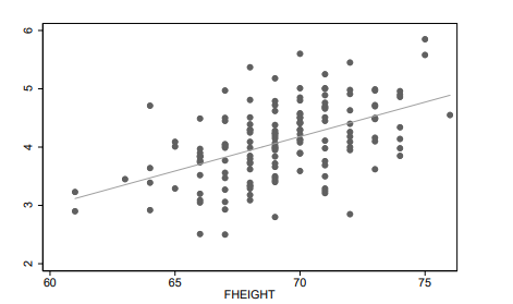
In Chapter 7 the data for fathers from the lung function data set were analyzed. These data fit the variable- $X$ case. Height was used as the $X$ variable in order to predict FEV1, and the following equation was obtained:
FEV1 $=-4.087+0.118$ (height in inches)
However, FEV1 tends to decrease with age for adults, so we should be able to predict it better if we use both height and age as independent variables in a multiple regression equation. We expect the slope coefficient for age to be negative and the slope coefficient for height to be positive.

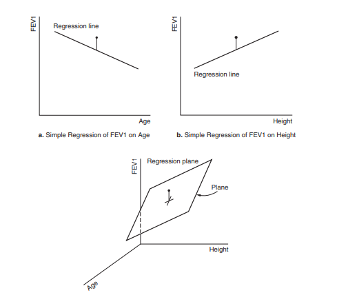
A geometric representation of the simple regression of FEV1 on age and height, respectively, is shown in Figures 8.1a and 8.1b. The multiple regression equation is represented by a plane, as shown in Figure 8.1c. Note that the plane slopes upward as a function of height and downward as a function of age. A hypothetical individual whose FEV1 is large relative to his age and height appears above both simple regression lines as well as above the multiple regression plane.

For illustration purposes Figure $8.2$ shows how a plane can be constructed. Constructing such a regression plane involves the following steps.

1. Draw lines on the $X_{1}, Y$ wall, setting $X_{2}=0$.
2. Draw lines on the $X_{2}, Y$ wall, setting $X_{1}=0$.
3. Drive nails in the walls at the lines drawn in steps 1 and 2 .
4. Connect the pairs of nails by strings and tighten the strings.
   The resulting strings in step 4 form a plane. This plane is the regression plane of $Y$ on $X_{1}$ and $X_{2}$. The mean of $Y$ at a given $X_{1}$ and $X_{2}$ is the point on the plane vertically above the point $X_{1}, X_{2}$.
   Data for the fathers in the lung function data set were analyzed by Stata. The following descriptive statistics were generated using the summarize command:
   $\begin{array}{lrrrrr}\text { Variable } & \text { Obs } & \text { Mean } & \text { Std.Dev } & \text { Minimum } & \text { Maximum } \ \text { Age } & 150 & 40.13 & 6.89 & 26.00 & 59.00 \ \text { Height } & 150 & 69.26 & 2.78 & 61.00 & 76.00 \ \text { FEV1 } & 150 & 4.09 & 0.65 & 2.50 & 5.85\end{array}$
   The regress command from Stata produced the following regression equation:
   $$
   \mathrm{FEV} 1=-2.761-0.027(\text { age })+0.114(\text { height })
   $$

统计代写|多元统计分析作业代写Multivariate Statistical Analysis代考|Regression methods: fixed- $X$ case

In this section we present the background assumptions, model, and formulas necessary for an understanding of multiple linear regression for the fixed- $X$ case. Computations can become tedious when there are several independent variables, so we assume that you will obtain output from a packaged computer program. Therefore we present a minimum of formulas and place the main emphasis on the techniques and interpretation of results. This section is slow reading and requires concentration.
Since there is more than one $X$ variable, we use the notation $X_{1}, X_{2}, \ldots, X_{P}$ to represent $P$ possible variables. In packaged programs these variables may appear in the output as $\mathbf{X}(1), \mathbf{X} 1$, VAR 1, etc. For the fixed- $X$ case, values of the $X$ variables are assumed to be fixed in advance in the sample. At each combination of levels of the $X$ variables, we conceptualize a distribution of the values of $Y$. This distribution of $Y$ values is assumed to have a mean value equal to $\alpha+\beta_{1} X_{1}+\beta_{2} X_{2}+\cdots+\beta_{P} X_{P}$ and a variance equal to $\sigma^{2}$ at given levels of $X_{1}, X_{2}, \ldots, X_{P}$.

假设检验代写

统计代写|多元统计分析作业代写Multivariate Statistical Analysis代考|Chapter outline

当研究人员希望检查单个因（结果）变量之间的关系时，执行多元回归和和一组独立（预测或解释）变量X1到X磷. 因变量和是连续型。这X变量通常也是连续的，尽管它们可以是离散的。

在部分8.2介绍了用于多元回归的两个基本模型，下一节给出了数据示例。固定的背景假设、模型和必要的公式X模型在部分给出8.4, 而部分8.5提供可用于变量的统计假设和附加公式-X模型。帮助解释固定的测试X模型在第8.6并且为变量提供了类似的信息-X第 8.7 节中的模型。部分8.8讨论了使用残差来评估模型是否合适并找出异常值。该部分给出了三种更改模型以使其更适合数据的方法：变换、多项式回归和交互项。定义了多重共线性，识别它的方法也在第 8.8 节中解释。部分8.9提供了执行回归分析时可用的其他几个选项，即通过原点回归、加权回归以及测试两个子组的回归是否相等。部分8.10讨论如何使用 Stata 和 SAS 获得本章中的数值结果，并包含一个表格，总结了本书中使用的软件程序中可用的选项。部分8.11解释了执行多元回归分析时要注意的事项。
本书中还有两章是关于多元线性回归分析的。第 9 章介绍了当研究者不确定模型中包含哪些变量时用于选择自变量或预测变量的方法。第 10 章讨论了缺失值和虚拟变量（当一些自变量是离散的时使用），并给出了处理多重共线性的方法。

统计代写|多元统计分析作业代写Multivariate Statistical Analysis代考|Data examplea

在第 7 章中，分析了来自肺功能数据集的父亲数据。这些数据符合变量-X案子。高度被用作X变量以预测 FEV1，并获得以下等式：
FEV1=−4.087+0.118（以英寸为单位的身高）
然而，对于成年人来说，FEV1 往往会随着年龄的增长而降低，因此如果我们在多元回归方程中同时使用身高和年龄作为自变量，我们应该能够更好地预测它。我们预计年龄的斜率系数为负，身高的斜率系数为正。

图 8.1a 和 8.1b 分别显示了 FEV1 对年龄和身高的简单回归的几何表示。多元回归方程用一个平面表示，如图 8.1c 所示。请注意，平面向上倾斜是高度的函数，向下倾斜是年龄的函数。FEV1 相对于他的年龄和身高较大的假设个体出现在简单回归线和多元回归平面之上。

出于说明目的图8.2展示了如何构建飞机。构建这样一个回归平面涉及以下步骤。

1. 在上面画线X1,和墙壁, 设置X2=0.
2. 在上面画线X2,和墙壁, 设置X1=0.
3. 在步骤 1 和 2 中绘制的线处将钉子钉入墙壁。
4. 用绳子连接成对的钉子并拉紧绳子。
   步骤 4 中生成的字符串形成一个平面。这个平面是回归平面和在X1和X2. 的平均值和在给定的X1和X2是平面上垂直于该点上方的点X1,X2.
   Stata分析了肺功能数据集中父亲的数据。使用 summarise 命令生成以下描述性统计信息：
    多变的  笔记  意思是  Std.Dev  最低限度  最大   年龄 15040.136.8926.0059.00  高度 15069.262.7861.0076.00  FEV1 1504.090.652.505.85
   来自 Stata 的回归命令产生以下回归方程：
   F和五1=−2.761−0.027( 年龄 )+0.114( 高度 )

统计代写|多元统计分析作业代写Multivariate Statistical Analysis代考|Regression methods: fixed-X案子

在本节中，我们将介绍理解固定-多元线性回归所必需的背景假设、模型和公式。X案子。当有多个自变量时，计算可能会变得乏味，因此我们假设您将从打包的计算机程序中获得输出。因此，我们提出了最少的公式，并将主要重点放在技术和结果的解释上。本节阅读速度较慢，需要集中注意力。
因为不止一个X变量，我们使用符号X1,X2,…,X磷代表磷可能的变量。在打包的程序中，这些变量可能会在输出中显示为X(1),X1，VAR 1等。对于固定-X的情况下，的值X假设变量在样本中是预先固定的。在每个级别的组合X变量，我们将值的分布概念化和. 这种分布和假定值的平均值等于一种+b1X1+b2X2+⋯+b磷X磷和方差等于σ2在给定的水平X1,X2,…,X磷.

统计代写请认准statistics-lab™. statistics-lab™为您的留学生涯保驾护航。

随机过程代考

在概率论概念中，随机过程是随机变量的集合。 若一随机系统的样本点是随机函数，则称此函数为样本函数，这一随机系统全部样本函数的集合是一个随机过程。 实际应用中，样本函数的一般定义在时间域或者空间域。 随机过程的实例如股票和汇率的波动、语音信号、视频信号、体温的变化，随机运动如布朗运动、随机徘徊等等。

贝叶斯方法代考

贝叶斯统计概念及数据分析表示使用概率陈述回答有关未知参数的研究问题以及统计范式。后验分布包括关于参数的先验分布，和基于观测数据提供关于参数的信息似然模型。根据选择的先验分布和似然模型，后验分布可以解析或近似，例如，马尔科夫链蒙特卡罗 (MCMC) 方法之一。贝叶斯统计概念及数据分析使用后验分布来形成模型参数的各种摘要，包括点估计，如后验平均值、中位数、百分位数和称为可信区间的区间估计。此外，所有关于模型参数的统计检验都可以表示为基于估计后验分布的概率报表。

广义线性模型代考

广义线性模型（GLM）归属统计学领域，是一种应用灵活的线性回归模型。该模型允许因变量的偏差分布有除了正态分布之外的其它分布。

statistics-lab作为专业的留学生服务机构，多年来已为美国、英国、加拿大、澳洲等留学热门地的学生提供专业的学术服务，包括但不限于Essay代写，Assignment代写，Dissertation代写，Report代写，小组作业代写，Proposal代写，Paper代写，Presentation代写，计算机作业代写，论文修改和润色，网课代做，exam代考等等。写作范围涵盖高中，本科，研究生等海外留学全阶段，辐射金融，经济学，会计学，审计学，管理学等全球99%专业科目。写作团队既有专业英语母语作者，也有海外名校硕博留学生，每位写作老师都拥有过硬的语言能力，专业的学科背景和学术写作经验。我们承诺100%原创，100%专业，100%准时，100%满意。

机器学习代写

随着AI的大潮到来，Machine Learning逐渐成为一个新的学习热点。同时与传统CS相比，Machine Learning在其他领域也有着广泛的应用，因此这门学科成为不仅折磨CS专业同学的“小恶魔”，也是折磨生物、化学、统计等其他学科留学生的“大魔王”。学习Machine learning的一大绊脚石在于使用语言众多，跨学科范围广，所以学习起来尤其困难。但是不管你在学习Machine Learning时遇到任何难题，StudyGate专业导师团队都能为你轻松解决。

多元统计分析代考

基础数据: $N$ 个样本， $P$ 个变量数的单样本，组成的横列的数据表
变量定性: 分类和顺序；变量定量：数值
数学公式的角度分为: 因变量与自变量

时间序列分析代写

随机过程，是依赖于参数的一组随机变量的全体，参数通常是时间。 随机变量是随机现象的数量表现，其时间序列是一组按照时间发生先后顺序进行排列的数据点序列。通常一组时间序列的时间间隔为一恒定值（如1秒，5分钟，12小时，7天，1年），因此时间序列可以作为离散时间数据进行分析处理。研究时间序列数据的意义在于现实中，往往需要研究某个事物其随时间发展变化的规律。这就需要通过研究该事物过去发展的历史记录，以得到其自身发展的规律。

回归分析代写

多元回归分析渐进（Multiple Regression Analysis Asymptotics）属于计量经济学领域，主要是一种数学上的统计分析方法，可以分析复杂情况下各影响因素的数学关系，在自然科学、社会和经济学等多个领域内应用广泛。

MATLAB代写

MATLAB 是一种用于技术计算的高性能语言。它将计算、可视化和编程集成在一个易于使用的环境中，其中问题和解决方案以熟悉的数学符号表示。典型用途包括：数学和计算算法开发建模、仿真和原型制作数据分析、探索和可视化科学和工程图形应用程序开发，包括图形用户界面构建MATLAB 是一个交互式系统，其基本数据元素是一个不需要维度的数组。这使您可以解决许多技术计算问题，尤其是那些具有矩阵和向量公式的问题，而只需用 C 或 Fortran 等标量非交互式语言编写程序所需的时间的一小部分。MATLAB 名称代表矩阵实验室。MATLAB 最初的编写目的是提供对由 LINPACK 和 EISPACK 项目开发的矩阵软件的轻松访问，这两个项目共同代表了矩阵计算软件的最新技术。MATLAB 经过多年的发展，得到了许多用户的投入。在大学环境中，它是数学、工程和科学入门和高级课程的标准教学工具。在工业领域，MATLAB 是高效研究、开发和分析的首选工具。MATLAB 具有一系列称为工具箱的特定于应用程序的解决方案。对于大多数 MATLAB 用户来说非常重要，工具箱允许您学习和应用专业技术。工具箱是 MATLAB 函数（M 文件）的综合集合，可扩展 MATLAB 环境以解决特定类别的问题。可用工具箱的领域包括信号处理、控制系统、神经网络、模糊逻辑、小波、仿真等。

如果你也在 怎样代写多元统计分析Multivariate Statistical Analysis这个学科遇到相关的难题，请随时右上角联系我们的24/7代写客服。

多变量统计分析Multivariate Statistical Analysis关注的是由一些个体或物体的测量数据集组成的数据。样本数据可能是从某个城市的学童群体中随机抽取的一些个体的身高和体重，或者对一组测量数据进行统计处理，例如从两个物种中抽取的鸢尾花花瓣的长度和宽度以及萼片的长度和宽度，或者我们可以研究对一些学生进行的智力测试的分数。
在一个特定的个体上，有p=#$的测量集合。
$n=#$ 观察值 $=$ 样本大小

statistics-lab™ 为您的留学生涯保驾护航 在代写多元统计分析Multivariate Statistical Analysis方面已经树立了自己的口碑, 保证靠谱, 高质且原创的统计Statistics代写服务。我们的专家在代写多元统计分析Multivariate Statistical Analysis代写方面经验极为丰富，各种代写多元统计分析Multivariate Statistical Analysis相关的作业也就用不着 说。

我们提供的多元统计分析Multivariate Statistical Analysis及其相关学科的代写，服务范围广, 其中包括但不限于:

• Statistical Inference 统计推断
• Statistical Computing 统计计算
• Advanced Probability Theory 高等楖率论
• Advanced Mathematical Statistics 高等数理统计学
• (Generalized) Linear Models 广义线性模型
• Statistical Machine Learning 统计机器学习
• Longitudinal Data Analysis 纵向数据 分析
• Foundations of Data Science 数据科学基础

统计代写|多元统计分析作业代写Multivariate Statistical Analysis代考|Why selection is often difficult

Simple linear regression analysis is commonly performed when investigators wish to examine the relationship between two variables. Section $7.2$ describes the two basic models used in linear regression analysis and a data example is given in Section 7.3. Section $7.4$ presents the assumptions, methodology, and usual output from the first model while Section $7.5$ does the same for the second model. Sections $7.6$ and $7.7$ discuss the interpretation of the results for the two models. In Section $7.8$ a variety of useful output options that are available from statistical programs are described. These outputs include standardized regression coefficients, the regression analysis of variance table, determining whether or not the relationship is linear, and how to find outliers and influential observations. Section $7.9$ defines robustness in statistical analysis and discusses how critical the various assumptions are. The use of transformations for simple linear regression is also described. In Section $7.10$ regression through the origin and weighted regression are introduced. How to obtain a loess curve and when it is used are also given in this section. In Section $7.11$ a variety of uses of linear regressions are presented. A brief discussion of how to obtain the computer output given in this chapter is found in Section $7.12$. Finally, Section $7.13$ describes what to watch out for in regression analysis.

If you are reading about simple linear regression for the first time, skip Sections 7.9, 7.10, and $7.11$ in your first reading. If this chapter is a review for you, you can skim most of it, but read the above-mentioned sections in detail.

统计代写|多元统计分析作业代写Multivariate Statistical Analysis代考|When are regression and correlation used?

The methods described in this chapter are appropriate for studying the relationship between two variables $X$ and $Y$. By convention, $X$ is called the independent or predictor variable and is plotted on the horizontal axis. The variable $Y$ is called the dependent or outcome variable and is plotted on the vertical axis. The dependent variable is assumed to be continuous, while the independent variable may be continuous or discrete.
The data for regression analysis can arise in two forms.

1. Fixed- $X$ case. The values of $X$ are selected by the researchers or forced on them by the nature of the situation. For example, in the problem of predicting the sales for a company, the total sales are given for each year. Year is the fixed- $X$ variable, and its values are imposed on the investigator by nature. In an experiment to determine the growth of a plant as a function of temperature, a researcher could randomly assign plants to three different preset temperatures that are maintained in three greenhouses. The three temperature values then become the fixed values for $X$.
2. Variable- $X$ case. The values of $X$ and $Y$ are both random variables. In this situation, cases are selected randomly from the population, and both $X$ and $Y$ are measured. All survey data are of this type, whereby individuals are chosen and various characteristics are measured on each.
   Regression and correlation analysis can be used for either of two main purposes.
3. Descriptive. The kind of relationship and its strength are examined.
   87
   88
   CHAPTER 7. SIMPLE REGRESSION AND CORRELATION
4. Predictive. The equation relating $Y$ and $X$ can be used to predict the value of $Y$ for a given value of $X$. Prediction intervals can also be used to indicate a likely range of the predicted value of $Y$.

统计代写|多元统计分析作业代写Multivariate Statistical Analysis代考|Data example

In this section we present an example used in the remainder of the chapter to illustrate the methods of regression and correlation. Lung function data were obtained from an epidemiological study of households living in four areas with different amounts and types of air pollution. The data set used in this book is a subset of the total data. In this chapter we use only the data taken on the fathers, all of whom are nonsmokers (see Appendix A for more details).

One of the major early indicators of reduced respiratory function is FEV1 or forced expiratory volume in the first second (amount of air exhaled in 1 second). Since it is known that taller males tend to have higher FEV1, we wish to determine the relationship between height and FEV1. We exclude the data from the mothers as several studies have shown a different relationship for women. The sample size is 150 . These data belong to the variable- $X$ case, where $X$ is height (in inches) and $Y$ is FEV1 (in liters). Here we may be concerned with describing the relationship between FEV1 and height, a descriptive purpose. We may also use the resulting equation to determine expected or normal FEV1 for a given height, a predictive use.

假设检验代写

统计代写|多元统计分析作业代写Multivariate Statistical Analysis代考|Why selection is often difficult

当调查人员希望检查两个变量之间的关系时，通常会进行简单的线性回归分析。部分7.2描述了线性回归分析中使用的两个基本模型，第 7.3 节给出了一个数据示例。部分7.4介绍了第一个模型的假设、方法和通常的输出，而第7.5对第二个模型做同样的事情。部分7.6和7.7讨论两个模型的结果的解释。在部分7.8描述了可从统计程序获得的各种有用的输出选项。这些输出包括标准化回归系数、方差表的回归分析、确定关系是否是线性的，以及如何找到异常值和有影响的观察值。部分7.9定义统计分析的稳健性并讨论各种假设的重要性。还描述了对简单线性回归的转换的使用。在部分7.10引入了原点回归和加权回归。本节还给出了如何获得黄土曲线以及何时使用它。在部分7.11介绍了线性回归的各种用途。关于如何获得本章给出的计算机输出的简要讨论见第 1 节。7.12. 最后，部分7.13描述了在回归分析中需要注意的事项。

如果您是第一次阅读简单线性回归，请跳过第 7.9、7.10 和7.11在你的第一次阅读中。如果本章是给您的复习，您可以略读大部分内容，但请详细阅读上述部分。

统计代写|多元统计分析作业代写Multivariate Statistical Analysis代考|When are regression and correlation used?

本章描述的方法适用于研究两个变量之间的关系X和和. 按照惯例，X称为自变量或预测变量，并绘制在水平轴上。变量和称为因变量或结果变量，并绘制在垂直轴上。假设因变量是连续的，而自变量可以是连续的或离散的。
回归分析的数据可以有两种形式。

1. 固定的-X案子。的价值观X由研究人员选择或根据情况的性质强加给他们。例如，在预测一家公司的销售额的问题中，给出了每年的总销售额。年份是固定的-X变量，它的值是天生强加给研究者的。在一项确定植物生长随温度变化的实验中，研究人员可以将植物随机分配到三个温室中保持的三个不同预设温度。然后三个温度值成为固定值X.
2. 多变的-X案子。的价值观X和和都是随机变量。在这种情况下，病例是从总体中随机选择的，并且X和和被测量。所有调查数据都属于这种类型，因此选择个人并测量每个人的各种特征。
   回归和相关分析可用于两个主要目的中的任何一个。
3. 描述性的。检查关系的类型及其强度。
   87
   88
   第 7 章简单的回归和相关
4. 预测性的。相关方程和和X可以用来预测值和对于给定的值X. 预测区间也可以用来表示预测值的可能范围和.

统计代写|多元统计分析作业代写Multivariate Statistical Analysis代考|Data example

在本节中，我们将展示本章其余部分中使用的示例来说明回归和相关的方法。肺功能数据来自对居住在空气污染程度和类型不同的四个地区的家庭进行的流行病学研究。本书中使用的数据集是总数据的一个子集。在本章中，我们仅使用父亲的数据，他们都是不吸烟者（更多详细信息请参见附录 A）。

呼吸功能降低的主要早期指标之一是第一秒内的 FEV1 或用力呼气量（1 秒内呼出的空气量）。由于已知较高的男性往往具有较高的 FEV1，因此我们希望确定身高与 FEV1 之间的关系。我们排除了母亲的数据，因为几项研究表明女性之间存在不同的关系。样本量为 150 。这些数据属于变量-X案例，在哪里X是高度（英寸）和和是 FEV1（升）。在这里，我们可能关心描述 FEV1 和身高之间的关系，这是一个描述性的目的。我们还可以使用得到的方程来确定给定高度的预期或正常 FEV1，这是一种预测用途。

统计代写请认准statistics-lab™. statistics-lab™为您的留学生涯保驾护航。

随机过程代考

在概率论概念中，随机过程是随机变量的集合。 若一随机系统的样本点是随机函数，则称此函数为样本函数，这一随机系统全部样本函数的集合是一个随机过程。 实际应用中，样本函数的一般定义在时间域或者空间域。 随机过程的实例如股票和汇率的波动、语音信号、视频信号、体温的变化，随机运动如布朗运动、随机徘徊等等。

贝叶斯方法代考

贝叶斯统计概念及数据分析表示使用概率陈述回答有关未知参数的研究问题以及统计范式。后验分布包括关于参数的先验分布，和基于观测数据提供关于参数的信息似然模型。根据选择的先验分布和似然模型，后验分布可以解析或近似，例如，马尔科夫链蒙特卡罗 (MCMC) 方法之一。贝叶斯统计概念及数据分析使用后验分布来形成模型参数的各种摘要，包括点估计，如后验平均值、中位数、百分位数和称为可信区间的区间估计。此外，所有关于模型参数的统计检验都可以表示为基于估计后验分布的概率报表。

广义线性模型代考

广义线性模型（GLM）归属统计学领域，是一种应用灵活的线性回归模型。该模型允许因变量的偏差分布有除了正态分布之外的其它分布。

statistics-lab作为专业的留学生服务机构，多年来已为美国、英国、加拿大、澳洲等留学热门地的学生提供专业的学术服务，包括但不限于Essay代写，Assignment代写，Dissertation代写，Report代写，小组作业代写，Proposal代写，Paper代写，Presentation代写，计算机作业代写，论文修改和润色，网课代做，exam代考等等。写作范围涵盖高中，本科，研究生等海外留学全阶段，辐射金融，经济学，会计学，审计学，管理学等全球99%专业科目。写作团队既有专业英语母语作者，也有海外名校硕博留学生，每位写作老师都拥有过硬的语言能力，专业的学科背景和学术写作经验。我们承诺100%原创，100%专业，100%准时，100%满意。

机器学习代写

随着AI的大潮到来，Machine Learning逐渐成为一个新的学习热点。同时与传统CS相比，Machine Learning在其他领域也有着广泛的应用，因此这门学科成为不仅折磨CS专业同学的“小恶魔”，也是折磨生物、化学、统计等其他学科留学生的“大魔王”。学习Machine learning的一大绊脚石在于使用语言众多，跨学科范围广，所以学习起来尤其困难。但是不管你在学习Machine Learning时遇到任何难题，StudyGate专业导师团队都能为你轻松解决。

多元统计分析代考

基础数据: $N$ 个样本， $P$ 个变量数的单样本，组成的横列的数据表
变量定性: 分类和顺序；变量定量：数值
数学公式的角度分为: 因变量与自变量

时间序列分析代写

随机过程，是依赖于参数的一组随机变量的全体，参数通常是时间。 随机变量是随机现象的数量表现，其时间序列是一组按照时间发生先后顺序进行排列的数据点序列。通常一组时间序列的时间间隔为一恒定值（如1秒，5分钟，12小时，7天，1年），因此时间序列可以作为离散时间数据进行分析处理。研究时间序列数据的意义在于现实中，往往需要研究某个事物其随时间发展变化的规律。这就需要通过研究该事物过去发展的历史记录，以得到其自身发展的规律。

回归分析代写

多元回归分析渐进（Multiple Regression Analysis Asymptotics）属于计量经济学领域，主要是一种数学上的统计分析方法，可以分析复杂情况下各影响因素的数学关系，在自然科学、社会和经济学等多个领域内应用广泛。

MATLAB代写

MATLAB 是一种用于技术计算的高性能语言。它将计算、可视化和编程集成在一个易于使用的环境中，其中问题和解决方案以熟悉的数学符号表示。典型用途包括：数学和计算算法开发建模、仿真和原型制作数据分析、探索和可视化科学和工程图形应用程序开发，包括图形用户界面构建MATLAB 是一个交互式系统，其基本数据元素是一个不需要维度的数组。这使您可以解决许多技术计算问题，尤其是那些具有矩阵和向量公式的问题，而只需用 C 或 Fortran 等标量非交互式语言编写程序所需的时间的一小部分。MATLAB 名称代表矩阵实验室。MATLAB 最初的编写目的是提供对由 LINPACK 和 EISPACK 项目开发的矩阵软件的轻松访问，这两个项目共同代表了矩阵计算软件的最新技术。MATLAB 经过多年的发展，得到了许多用户的投入。在大学环境中，它是数学、工程和科学入门和高级课程的标准教学工具。在工业领域，MATLAB 是高效研究、开发和分析的首选工具。MATLAB 具有一系列称为工具箱的特定于应用程序的解决方案。对于大多数 MATLAB 用户来说非常重要，工具箱允许您学习和应用专业技术。工具箱是 MATLAB 函数（M 文件）的综合集合，可扩展 MATLAB 环境以解决特定类别的问题。可用工具箱的领域包括信号处理、控制系统、神经网络、模糊逻辑、小波、仿真等。

如果你也在 怎样代写多元统计分析Multivariate Statistical Analysis这个学科遇到相关的难题，请随时右上角联系我们的24/7代写客服。

多变量统计分析Multivariate Statistical Analysis关注的是由一些个体或物体的测量数据集组成的数据。样本数据可能是从某个城市的学童群体中随机抽取的一些个体的身高和体重，或者对一组测量数据进行统计处理，例如从两个物种中抽取的鸢尾花花瓣的长度和宽度以及萼片的长度和宽度，或者我们可以研究对一些学生进行的智力测试的分数。
在一个特定的个体上，有p=#$的测量集合。
$n=#$ 观察值 $=$ 样本大小

statistics-lab™ 为您的留学生涯保驾护航 在代写多元统计分析Multivariate Statistical Analysis方面已经树立了自己的口碑, 保证靠谱, 高质且原创的统计Statistics代写服务。我们的专家在代写多元统计分析Multivariate Statistical Analysis代写方面经验极为丰富，各种代写多元统计分析Multivariate Statistical Analysis相关的作业也就用不着 说。

我们提供的多元统计分析Multivariate Statistical Analysis及其相关学科的代写，服务范围广, 其中包括但不限于:

• Statistical Inference 统计推断
• Statistical Computing 统计计算
• Advanced Probability Theory 高等楖率论
• Advanced Mathematical Statistics 高等数理统计学
• (Generalized) Linear Models 广义线性模型
• Statistical Machine Learning 统计机器学习
• Longitudinal Data Analysis 纵向数据 分析
• Foundations of Data Science 数据科学基础

统计代写|多元统计分析作业代写Multivariate Statistical Analysis代考|Why selection is often difficult

There are two reasons why deciding what descriptive measures or analyses to perform and report is often difficult for an investigator with real-life data. First, in statistics textbooks, statistical methods are presented in a logical order from the viewpoint of learning statistics but not from the viewpoint of doing data analysis by using statistics. Most texts are either mathematical statistics texts, or are imitations of them with the mathematics simplified or left out. Also, when learning statistics for the first time, the student often finds mastering the techniques themselves tough enough without worrying about how to use them in the future. The second reason is that real-life data often contain mixtures of types of data, which makes the choice of analysis somewhat arbitrary. Two trained statisticians presented with the same set of data will often opt for different ways of analyzing the set, depending on what assumptions they are willing to take into account in the interpretation of the analysis.

Acquiring a sense of when it is safe to ignore assumptions is difficult both to learn and to teach. Here, for the most part, an empirical approach will be suggested. For example, it is often a good idea to perform several different analyses, one where all the assumptions are met and one where some are not, and compare the results. The idea is to use statistics to obtain insights into the data and to determine how the system under study works.

One point to keep in mind is that the examples presented in many statistics books are often ones the authors have selected after a long period of working with a particular technique. Thus they usually are “ideal” examples, designed to suit the technique being discussed. This feature makes learning the technique simpler but does not provide insight into its use in typical real-life situations. In this book we will attempt to be more flexible than standard textbooks so that you will gain experience with commonly encountered difficulties.

统计代写|多元统计分析作业代写Multivariate Statistical Analysis代考|Appropriate statistical measures

Suitable graphical measures for nominal data are bar graphs and pie charts. These bar graphs and pie charts show the proportion of respondents who have each of the five responses for religion. The length of the bar represents the proportion for the bar graph and the size (or angle) of the piece represents the proportion for the pie chart. Fox and Long (1990) note that both of these graphical methods can be successfully used by observers to make estimates of proportions or counts. Others are less impressed with the so-called stacked bar graphs (where each bar is divided into a number of subdistances based on another variable, say gender). It is difficult to compare the subdistances in stacked bar graphs since they all do not start at a common base. Bar graphs and pie charts are available in all four packages.

Note that there are two types of pie charts: the “value” and the “count” pie charts. Some packages only have the former. The count pie chart has a pie piece corresponding to each category of a given variable. On the other hand, the value pie charts represent the sum of values for each of a group of

统计代写|多元统计分析作业代写Multivariate Statistical Analysis代考|Selecting appropriate multivariate analyses

To decide on possible analyses, we can classify variables as follows:

1. independent versus dependent;
2. nominal or ordinal versus interval or ratio.
   The classification of independent or dependent may differ from analysis to analysis, but the classification into Stevens’s system usually remains constant throughout the analysis phase of the study. Once these classifications are determined, it is possible to refer to Table $6.2$ and decide what analysis should be considered. This table should be used as a general guide to analysis selection rather than as a strict set of rules.

In Table $6.2$ nominal and ordinal variables have been combined because this book does not cover analyses appropriate only to nominal or ordinal data separately. An extensive summary of measures and tests for these types of variables is given in Xie and Powers (2008) and Agresti (2012). Interval and ratio variables have also been combined because the same analyses are used for both types of variables. There are many measures of association and many statistical methods not listed in the table. For further information on choosing analyses appropriate to various data types, see Andrews et al. (1998).

The first row in the body of Table $6.2$ includes analyses that can be done if there are no dependent variables. Note that if there is only one variable, it can be considered either dependent or independent. A single independent variable that is either interval or ratio can be screened by methods given in Chapters 3 and 4 , and descriptive statistics can be obtained from many statistical programs. If there are several interval or ratio independent variables, then several techniques are listed in the table.

假设检验代写

统计代写|多元统计分析作业代写Multivariate Statistical Analysis代考|Why selection is often difficult

对于拥有真实数据的调查人员来说，决定执行和报告哪些描述性措施或分析通常很困难有两个原因。首先，在统计学教科书中，统计学方法是从学习统计学的角度按逻辑顺序呈现的，而不是从使用统计学进行数据分析的角度。大多数课本要么是数理统计课本，要么是对其进行数学简化或省略的模仿。此外，在第一次学习统计数据时，学生通常会发现自己掌握这些技术已经足够困难，而不必担心将来如何使用它们。第二个原因是现实生活中的数据通常包含混合类型的数据，这使得分析的选择有些随意。

了解什么时候可以安全地忽略假设是很难学习和教授的。在这里，在大多数情况下，将建议一种经验方法。例如，执行几种不同的分析通常是一个好主意，一种是满足所有假设，另一种是不满足一些假设，然后比较结果。这个想法是使用统计数据来获得对数据的洞察力，并确定所研究的系统是如何工作的。

需要记住的一点是，许多统计书籍中提供的示例通常是作者在长时间使用特定技术后选择的示例。因此，它们通常是“理想的”示例，旨在适应所讨论的技术。此功能使学习该技术更简单，但无法深入了解其在典型现实生活中的使用情况。在本书中，我们将尝试比标准教科书更灵活，以便您获得解决常见困难的经验。

统计代写|多元统计分析作业代写Multivariate Statistical Analysis代考|Appropriate statistical measures

适用于标称数据的图形度量是条形图和饼图。这些条形图和饼图显示了对宗教有五种回答的受访者的比例。条的长度代表条形图的比例，块的大小（或角度）代表饼图的比例。Fox 和 Long (1990) 指出，观察者可以成功地使用这两种图形方法来估计比例或计数。其他人对所谓的堆叠条形图（其中每个条形图根据另一个变量（例如性别）划分为多个子距离）印象不深。很难比较堆叠条形图中的子距离，因为它们都不是从一个共同的基础开始的。所有四个软件包都提供条形图和饼图。

请注意，有两种类型的饼图：“值”饼图和“计数”饼图。有些包只有前者。计数饼图具有对应于给定变量的每个类别的饼图。另一方面，值饼图表示一组中每一个的值的总和

统计代写|多元统计分析作业代写Multivariate Statistical Analysis代考|Selecting appropriate multivariate analyses

为了决定可能的分析，我们可以将变量分类如下：

1. 独立与依赖；
2. 名义或有序与区间或比率。
   独立或依赖的分类可能因分析而异，但史蒂文斯系统的分类通常在整个研究的分析阶段保持不变。一旦确定了这些分类，就可以参考表6.2并决定应该考虑什么分析。此表应用作分析选择的一般指南，而不是一套严格的规则。

在表中6.2名义变量和有序变量已合并，因为本书不涵盖仅适用于单独的名义或有序数据的分析。Xie and Powers (2008) 和 Agresti (2012) 对这些类型变量的测量和测试进行了广泛的总结。区间和比率变量也被合并，因为这两种类型的变量都使用了相同的分析。表中没有列出许多关联度量和许多统计方法。有关选择适合各种数据类型的分析的更多信息，请参阅 Andrews 等人。（1998 年）。

表格正文中的第一行6.2包括在没有因变量的情况下可以进行的分析。请注意，如果只有一个变量，则可以将其视为依赖变量或独立变量。可以通过第 3 章和第 4 章给出的方法筛选单个自变量，无论是区间还是比率，并且可以从许多统计程序中获得描述性统计。如果有多个区间或比率自变量，则表中列出了几种技术。

统计代写请认准statistics-lab™. statistics-lab™为您的留学生涯保驾护航。

随机过程代考

在概率论概念中，随机过程是随机变量的集合。 若一随机系统的样本点是随机函数，则称此函数为样本函数，这一随机系统全部样本函数的集合是一个随机过程。 实际应用中，样本函数的一般定义在时间域或者空间域。 随机过程的实例如股票和汇率的波动、语音信号、视频信号、体温的变化，随机运动如布朗运动、随机徘徊等等。

贝叶斯方法代考

贝叶斯统计概念及数据分析表示使用概率陈述回答有关未知参数的研究问题以及统计范式。后验分布包括关于参数的先验分布，和基于观测数据提供关于参数的信息似然模型。根据选择的先验分布和似然模型，后验分布可以解析或近似，例如，马尔科夫链蒙特卡罗 (MCMC) 方法之一。贝叶斯统计概念及数据分析使用后验分布来形成模型参数的各种摘要，包括点估计，如后验平均值、中位数、百分位数和称为可信区间的区间估计。此外，所有关于模型参数的统计检验都可以表示为基于估计后验分布的概率报表。

广义线性模型代考

广义线性模型（GLM）归属统计学领域，是一种应用灵活的线性回归模型。该模型允许因变量的偏差分布有除了正态分布之外的其它分布。

statistics-lab作为专业的留学生服务机构，多年来已为美国、英国、加拿大、澳洲等留学热门地的学生提供专业的学术服务，包括但不限于Essay代写，Assignment代写，Dissertation代写，Report代写，小组作业代写，Proposal代写，Paper代写，Presentation代写，计算机作业代写，论文修改和润色，网课代做，exam代考等等。写作范围涵盖高中，本科，研究生等海外留学全阶段，辐射金融，经济学，会计学，审计学，管理学等全球99%专业科目。写作团队既有专业英语母语作者，也有海外名校硕博留学生，每位写作老师都拥有过硬的语言能力，专业的学科背景和学术写作经验。我们承诺100%原创，100%专业，100%准时，100%满意。

机器学习代写

随着AI的大潮到来，Machine Learning逐渐成为一个新的学习热点。同时与传统CS相比，Machine Learning在其他领域也有着广泛的应用，因此这门学科成为不仅折磨CS专业同学的“小恶魔”，也是折磨生物、化学、统计等其他学科留学生的“大魔王”。学习Machine learning的一大绊脚石在于使用语言众多，跨学科范围广，所以学习起来尤其困难。但是不管你在学习Machine Learning时遇到任何难题，StudyGate专业导师团队都能为你轻松解决。

多元统计分析代考

基础数据: $N$ 个样本， $P$ 个变量数的单样本，组成的横列的数据表
变量定性: 分类和顺序；变量定量：数值
数学公式的角度分为: 因变量与自变量

时间序列分析代写

随机过程，是依赖于参数的一组随机变量的全体，参数通常是时间。 随机变量是随机现象的数量表现，其时间序列是一组按照时间发生先后顺序进行排列的数据点序列。通常一组时间序列的时间间隔为一恒定值（如1秒，5分钟，12小时，7天，1年），因此时间序列可以作为离散时间数据进行分析处理。研究时间序列数据的意义在于现实中，往往需要研究某个事物其随时间发展变化的规律。这就需要通过研究该事物过去发展的历史记录，以得到其自身发展的规律。

回归分析代写

多元回归分析渐进（Multiple Regression Analysis Asymptotics）属于计量经济学领域，主要是一种数学上的统计分析方法，可以分析复杂情况下各影响因素的数学关系，在自然科学、社会和经济学等多个领域内应用广泛。

MATLAB代写

MATLAB 是一种用于技术计算的高性能语言。它将计算、可视化和编程集成在一个易于使用的环境中，其中问题和解决方案以熟悉的数学符号表示。典型用途包括：数学和计算算法开发建模、仿真和原型制作数据分析、探索和可视化科学和工程图形应用程序开发，包括图形用户界面构建MATLAB 是一个交互式系统，其基本数据元素是一个不需要维度的数组。这使您可以解决许多技术计算问题，尤其是那些具有矩阵和向量公式的问题，而只需用 C 或 Fortran 等标量非交互式语言编写程序所需的时间的一小部分。MATLAB 名称代表矩阵实验室。MATLAB 最初的编写目的是提供对由 LINPACK 和 EISPACK 项目开发的矩阵软件的轻松访问，这两个项目共同代表了矩阵计算软件的最新技术。MATLAB 经过多年的发展，得到了许多用户的投入。在大学环境中，它是数学、工程和科学入门和高级课程的标准教学工具。在工业领域，MATLAB 是高效研究、开发和分析的首选工具。MATLAB 具有一系列称为工具箱的特定于应用程序的解决方案。对于大多数 MATLAB 用户来说非常重要，工具箱允许您学习和应用专业技术。工具箱是 MATLAB 函数（M 文件）的综合集合，可扩展 MATLAB 环境以解决特定类别的问题。可用工具箱的领域包括信号处理、控制系统、神经网络、模糊逻辑、小波、仿真等。

如果你也在 怎样代写多元统计分析Multivariate Statistical Analysis这个学科遇到相关的难题，请随时右上角联系我们的24/7代写客服。

多变量统计分析Multivariate Statistical Analysis关注的是由一些个体或物体的测量数据集组成的数据。样本数据可能是从某个城市的学童群体中随机抽取的一些个体的身高和体重，或者对一组测量数据进行统计处理，例如从两个物种中抽取的鸢尾花花瓣的长度和宽度以及萼片的长度和宽度，或者我们可以研究对一些学生进行的智力测试的分数。
在一个特定的个体上，有p=#$的测量集合。
$n=#$ 观察值 $=$ 样本大小

statistics-lab™ 为您的留学生涯保驾护航 在代写多元统计分析Multivariate Statistical Analysis方面已经树立了自己的口碑, 保证靠谱, 高质且原创的统计Statistics代写服务。我们的专家在代写多元统计分析Multivariate Statistical Analysis代写方面经验极为丰富，各种代写多元统计分析Multivariate Statistical Analysis相关的作业也就用不着 说。

我们提供的多元统计分析Multivariate Statistical Analysis及其相关学科的代写，服务范围广, 其中包括但不限于:

• Statistical Inference 统计推断
• Statistical Computing 统计计算
• Advanced Probability Theory 高等楖率论
• Advanced Mathematical Statistics 高等数理统计学
• (Generalized) Linear Models 广义线性模型
• Statistical Machine Learning 统计机器学习
• Longitudinal Data Analysis 纵向数据 分析
• Foundations of Data Science 数据科学基础

统计代写|多元统计分析作业代写Multivariate Statistical Analysis代考|Transformations, assessing normality and independence

In Section $3.4$ we discussed the use of transformations to create new variables. In this chapter we discuss transforming the data to obtain a distribution that is approximately normal. This is of particular interest for exploratory data analysis. For confirmatory data analysis (as described in Chapter 1) one should choose any appropriate transformations of variables prior to performing any analyses. Section $5.2$ shows how transformations change the shape of distributions. Section $5.3$ discusses several methods for deciding when a transformation should be made and how to find a suitable transformation. An iterative scheme is proposed that helps to zero in on a good transformation and statistical tests for normality are evaluated. Section $5.4$ presents simple graphical methods for determining if the data are independent. Section $5.5$ provides an overview of the methods used in the four statistical software packages for topics discussed in this chapter. In this chapter, we rely heavily on graphical methods: see Cook and Weisberg (1994) and Tufte (2001).

Each computer software package offers the users information to help decide if their data are normally distributed. The packages provide convenient methods for transforming the data to achieve approximate normality. They also include some output for checking the independence of the observations. Hence the assumption of independent, normally distributed data that is made in many statistical tests can be assessed, at least approximately. Note that it has been shown that inference can be robust in many research settings even with highly non-normal data (see Lumley et al., 2002). Additionally, many investigators may try to discard the most obvious outliers prior to assessing normality because such outliers can grossly distort the distribution, but discarding outliers is generally not advised unless it is concluded that an error has occurred in the measurement, recording or entry of these observations. Some researchers also consider removing inconsistent or extreme observations (see Osborne and Overbay, 2004), but such a decision depends heavily on the circumstances surrounding the research topic and should always be documented.

统计代写|多元统计分析作业代写Multivariate Statistical Analysis代考|Common transformations

For exploratory analysis of data it may be useful to transform certain variables before performing the analyses. Examples are found in the next section and in Chapter 7. In this section we present some common transformations. If you are familiar with this subject, you may wish to skip to the next section.

To develop a feel for transformations, let us examine a plot of transformed values versus the original values of the variable. To begin with, a plot of values of a variable $X$ against itself produces a $45^{\circ}$ diagonal line going through the origin, as shown in Figure 5.1.

One of the most commonly performed transformations is taking the logarithm (log) to base 10 . Recall that the logarithm is the number that satisfies the relationship $X=10^{Y}$. That is, the logarithm of $X$ is the power $Y$ to which 10 must be raised in order to produce $X$. As shown in Figure $5.2$ in plot a, the logarithm of 10 is 1 since $10=10^{1}$. Similarly, the logarithm of 1 is 0 since $1=10^{\circ}$, and the logarithm of 100 is 2 since $100=10^{2}$. Other values of logarithms can be obtained from tables of common logarithms, from a hand calculator with a log function, or from statistical packages by using the transformation options. All statistical packages discussed in this book allow the user to make this transformation as well as others.

统计代写|多元统计分析作业代写Multivariate Statistical Analysis代考|Selecting appropriate transformations

In the theoretical development of statistical methods some assumptions might be made regarding the distribution of the variables being analyzed. The most commonly assumed distribution for continuous observations is the normal, or Gaussian, distribution. Nevertheless, even if the values of a variable are not or are far from being normally distributed, the averages of such data can be shown to be normally distributed for large enough sample sizes. This is a pivotal mathematical result called the Central Limit Theorem. For a review and discussion of what sample size can be considered “large enough” in relation to highly non-normal data see Lumley et al. (2002). In this section, methods for assessing normality and for choosing a transformation to induce normality are presented.
Assessing normality using histograms
The left graph of Figure 5.4a illustrates the appearance of an ideal histogram, or density function, of normally distributed data. The values of the variable $X$ are plotted on the horizontal axis. The range of $X$ is partitioned into numerous intervals of equal length and the proportion of observations in each interval is plotted on the vertical axis (see also Section 4.2). The mean is in the center of the distribution and is equal to zero in this hypothetical histogram. The distribution is symmetric about the mean; that is, intervals equidistant from the mean have equal proportions of observations (or the same height in the histogram). If you place a mirror vertically at the mean of a symmetric histogram, the right side should be a mirror image of the left side. A distribution may be symmetric and still.

假设检验代写

统计代写|多元统计分析作业代写Multivariate Statistical Analysis代考|Transformations, assessing normality and independence

在部分3.4我们讨论了使用转换来创建新变量。在本章中，我们讨论如何转换数据以获得近似正态分布。这对于探索性数据分析特别感兴趣。对于验证性数据分析（如第 1 章所述），应在执行任何分析之前选择任何适当的变量转换。部分5.2显示变换如何改变分布的形状。部分5.3讨论了决定何时进行转换以及如何找到合适的转换的几种方法。提出了一种迭代方案，有助于将良好的转换归零，并评估正态性的统计测试。部分5.4提供了用于确定数据是否独立的简单图形方法。部分5.5概述了本章讨论的主题的四个统计软件包中使用的方法。在本章中，我们严重依赖图形方法：参见 Cook 和 Weisberg (1994) 和 Tufte (2001)。

每个计算机软件包都为用户提供信息，以帮助确定他们的数据是否正常分布。这些包提供了转换数据以实现近似正态性的便捷方法。它们还包括一些用于检查观察独立性的输出。因此，可以至少近似地评估在许多统计测试中做出的独立、正态分布数据的假设。请注意，已经表明，即使使用高度非正态的数据，推理在许多研究环境中也是稳健的（参见 Lumley 等人，2002 年）。此外，许多调查人员可能会在评估正态性之前尝试丢弃最明显的异常值，因为这些异常值会严重扭曲分布，但通常不建议丢弃异常值，除非得出结论认为在这些观察结果的测量、记录或输入中发生了错误。一些研究人员还考虑删除不一致或极端的观察结果（参见 Osborne 和 Overbay，2004 年），但这样的决定很大程度上取决于围绕研究主题的情况，并且应始终记录在案。

统计代写|多元统计分析作业代写Multivariate Statistical Analysis代考|Common transformations

对于数据的探索性分析，在执行分析之前转换某些变量可能很有用。示例在下一节和第 7 章中找到。在本节中，我们将介绍一些常见的转换。如果您熟悉此主题，您可能希望跳到下一部分。

为了培养对转换的感觉，让我们检查转换值与变量原始值的关系图。首先，一个变量的值图X对自己产生一个45∘对角线穿过原点，如图 5.1 所示。

最常执行的转换之一是将对数 (log) 以 10 为底。回想一下，对数是满足关系的数X=10和. 也就是说，对数X是权力和必须提高到 10 才能生产X. 如图5.2在图 a 中，10 的对数为 1，因为10=101. 同样，1 的对数为 0，因为1=10∘, 100 的对数是 2100=102. 其他对数值可以从常用对数表、具有对数功能的手动计算器或使用转换选项从统计包中获得。本书中讨论的所有统计软件包都允许用户进行这种转换以及其他转换。

统计代写|多元统计分析作业代写Multivariate Statistical Analysis代考|Selecting appropriate transformations

在统计方法的理论发展中，可能会对所分析的变量的分布做出一些假设。连续观测最常见的假设分布是正态分布或高斯分布。然而，即使变量的值不是正态分布或远非正态分布，对于足够大的样本量，这些数据的平均值也可以显示为正态分布。这是一个关键的数学结果，称为中心极限定理。有关与高度非正态数据相关的样本量可以被视为“足够大”的审查和讨论，请参见 Lumley 等人。（2002 年）。在本节中，介绍了评估正态性和选择转换以诱导正态性的方法。
使用直方图评估正态性
图 5.4a 的左图说明了正态分布数据的理想直方图或密度函数的外观。变量的值X绘制在水平轴上。的范围X被划分为许多等长的区间，并且每个区间中的观察比例绘制在垂直轴上（另见第 4.2 节）。均值位于分布的中心，在此假设直方图中为零。分布关于均值对称；也就是说，与平均值等距的区间具有相同比例的观测值（或直方图中的相同高度）。如果在对称直方图的平均值上垂直放置镜子，则右侧应该是左侧的镜像。分布可能是对称且静止的。

统计代写请认准statistics-lab™. statistics-lab™为您的留学生涯保驾护航。

随机过程代考

在概率论概念中，随机过程是随机变量的集合。 若一随机系统的样本点是随机函数，则称此函数为样本函数，这一随机系统全部样本函数的集合是一个随机过程。 实际应用中，样本函数的一般定义在时间域或者空间域。 随机过程的实例如股票和汇率的波动、语音信号、视频信号、体温的变化，随机运动如布朗运动、随机徘徊等等。

贝叶斯方法代考

贝叶斯统计概念及数据分析表示使用概率陈述回答有关未知参数的研究问题以及统计范式。后验分布包括关于参数的先验分布，和基于观测数据提供关于参数的信息似然模型。根据选择的先验分布和似然模型，后验分布可以解析或近似，例如，马尔科夫链蒙特卡罗 (MCMC) 方法之一。贝叶斯统计概念及数据分析使用后验分布来形成模型参数的各种摘要，包括点估计，如后验平均值、中位数、百分位数和称为可信区间的区间估计。此外，所有关于模型参数的统计检验都可以表示为基于估计后验分布的概率报表。

广义线性模型代考

广义线性模型（GLM）归属统计学领域，是一种应用灵活的线性回归模型。该模型允许因变量的偏差分布有除了正态分布之外的其它分布。

statistics-lab作为专业的留学生服务机构，多年来已为美国、英国、加拿大、澳洲等留学热门地的学生提供专业的学术服务，包括但不限于Essay代写，Assignment代写，Dissertation代写，Report代写，小组作业代写，Proposal代写，Paper代写，Presentation代写，计算机作业代写，论文修改和润色，网课代做，exam代考等等。写作范围涵盖高中，本科，研究生等海外留学全阶段，辐射金融，经济学，会计学，审计学，管理学等全球99%专业科目。写作团队既有专业英语母语作者，也有海外名校硕博留学生，每位写作老师都拥有过硬的语言能力，专业的学科背景和学术写作经验。我们承诺100%原创，100%专业，100%准时，100%满意。

机器学习代写

随着AI的大潮到来，Machine Learning逐渐成为一个新的学习热点。同时与传统CS相比，Machine Learning在其他领域也有着广泛的应用，因此这门学科成为不仅折磨CS专业同学的“小恶魔”，也是折磨生物、化学、统计等其他学科留学生的“大魔王”。学习Machine learning的一大绊脚石在于使用语言众多，跨学科范围广，所以学习起来尤其困难。但是不管你在学习Machine Learning时遇到任何难题，StudyGate专业导师团队都能为你轻松解决。

多元统计分析代考

基础数据: $N$ 个样本， $P$ 个变量数的单样本，组成的横列的数据表
变量定性: 分类和顺序；变量定量：数值
数学公式的角度分为: 因变量与自变量

时间序列分析代写

随机过程，是依赖于参数的一组随机变量的全体，参数通常是时间。 随机变量是随机现象的数量表现，其时间序列是一组按照时间发生先后顺序进行排列的数据点序列。通常一组时间序列的时间间隔为一恒定值（如1秒，5分钟，12小时，7天，1年），因此时间序列可以作为离散时间数据进行分析处理。研究时间序列数据的意义在于现实中，往往需要研究某个事物其随时间发展变化的规律。这就需要通过研究该事物过去发展的历史记录，以得到其自身发展的规律。

回归分析代写

多元回归分析渐进（Multiple Regression Analysis Asymptotics）属于计量经济学领域，主要是一种数学上的统计分析方法，可以分析复杂情况下各影响因素的数学关系，在自然科学、社会和经济学等多个领域内应用广泛。

MATLAB代写

MATLAB 是一种用于技术计算的高性能语言。它将计算、可视化和编程集成在一个易于使用的环境中，其中问题和解决方案以熟悉的数学符号表示。典型用途包括：数学和计算算法开发建模、仿真和原型制作数据分析、探索和可视化科学和工程图形应用程序开发，包括图形用户界面构建MATLAB 是一个交互式系统，其基本数据元素是一个不需要维度的数组。这使您可以解决许多技术计算问题，尤其是那些具有矩阵和向量公式的问题，而只需用 C 或 Fortran 等标量非交互式语言编写程序所需的时间的一小部分。MATLAB 名称代表矩阵实验室。MATLAB 最初的编写目的是提供对由 LINPACK 和 EISPACK 项目开发的矩阵软件的轻松访问，这两个项目共同代表了矩阵计算软件的最新技术。MATLAB 经过多年的发展，得到了许多用户的投入。在大学环境中，它是数学、工程和科学入门和高级课程的标准教学工具。在工业领域，MATLAB 是高效研究、开发和分析的首选工具。MATLAB 具有一系列称为工具箱的特定于应用程序的解决方案。对于大多数 MATLAB 用户来说非常重要，工具箱允许您学习和应用专业技术。工具箱是 MATLAB 函数（M 文件）的综合集合，可扩展 MATLAB 环境以解决特定类别的问题。可用工具箱的领域包括信号处理、控制系统、神经网络、模糊逻辑、小波、仿真等。

如果你也在 怎样代写多元统计分析Multivariate Statistical Analysis这个学科遇到相关的难题，请随时右上角联系我们的24/7代写客服。

多变量统计分析Multivariate Statistical Analysis关注的是由一些个体或物体的测量数据集组成的数据。样本数据可能是从某个城市的学童群体中随机抽取的一些个体的身高和体重，或者对一组测量数据进行统计处理，例如从两个物种中抽取的鸢尾花花瓣的长度和宽度以及萼片的长度和宽度，或者我们可以研究对一些学生进行的智力测试的分数。
在一个特定的个体上，有p=#$的测量集合。
$n=#$ 观察值 $=$ 样本大小

statistics-lab™ 为您的留学生涯保驾护航 在代写多元统计分析Multivariate Statistical Analysis方面已经树立了自己的口碑, 保证靠谱, 高质且原创的统计Statistics代写服务。我们的专家在代写多元统计分析Multivariate Statistical Analysis代写方面经验极为丰富，各种代写多元统计分析Multivariate Statistical Analysis相关的作业也就用不着 说。

我们提供的多元统计分析Multivariate Statistical Analysis及其相关学科的代写，服务范围广, 其中包括但不限于:

• Statistical Inference 统计推断
• Statistical Computing 统计计算
• Advanced Probability Theory 高等楖率论
• Advanced Mathematical Statistics 高等数理统计学
• (Generalized) Linear Models 广义线性模型
• Statistical Machine Learning 统计机器学习
• Longitudinal Data Analysis 纵向数据 分析
• Foundations of Data Science 数据科学基础

统计代写|多元统计分析作业代写Multivariate Statistical Analysis代考|Introduction

Visualizing data is one of the most important things we can do to become familiar with the data. There are often features and patterns in the data that cannot be uncovered with summary statistics alone. There tend to be two forms in which data can be presented; Summary tables are used for comparing exact values between groups for example, and plots for conveying trends and patterns when exact numbers are not always necessary to convey a story. This chapter introduces a series of plot types for both categorical and continuous data. We start with visualizations for a single variable only (univariate), then combinations of two variables (bivariate), and lastly a few examples and discussion of methods for exploring relationships between more than two variables (multivariate). Additional graphs designed for a specific analysis setting are introduced as needed in other chapters of this book.

This chapter uses several data sets described in Appendix A. Specifically, we use the parental HIV and the depression data sets to demonstrate different visualization techniques. Almost all graphics in this chapter are made using R, with Section $4.5$ containing a discussion of graphical capabilities to create these graphs in other statistical software programs.

There are three levels of visualizations that can be created, with examples shown in Figure 4.1a, b and $\mathrm{c}$.

• For your eyes only (4.1a): Made by the analyst, for the analyst, these plots are quick and easy to create, using the default options without any annotation or context. These graphs are meant to be looked at once or twice for exploratory analysis in order to better understand the data.
• For an internal report (4.1b): Some chosen plots are then cleaned up to be shared with others, for example in a weekly team meeting or to be sent to co-investigators participating in the study. These plots need to be capable of standing on their own, but can be slightly less than perfect. Axis labels, titles, colors, annotations and other captions are provided as needed to put the graph in context.
• For publication or external report (4.1c): These are meant to be shared with other stakeholders such as the public, your collaborator(s) or administration. Very few plots make it this far. These plots should have all the “bells and whistles” as they appear in formal reports, and are often saved to an external file of a specific size or file type, with high resolution. For publication in most printed journals and books, figures typically need to be in black and white (possibly grayscale).
  Along with having the audience in mind, it is important to give thought to the purpose of the chart. “The effectiveness of any visualization can be measured according to how well it fulfills the tasks it was designed for.” (A. Cairo, personal communication, Aug 9, 2018).

统计代写|多元统计分析作业代写Multivariate Statistical Analysis代考|UNIVARIATE DATA

Because stem-leaf plots display the value of every observation in the data set, the data values can be read directly. The first row displays data from 15 to 19 years of age, or, the second half of the 10 s place. Note that this study enrolled only adults, so the youngest possible age is 18 . There are five 18 year olds and five 19 year olds in the data set. From this plot one can get an idea of how the data are distributed and know the actual values (of ages in this example). The second row displays data on ages between 20 and 24 , or the first half of the $20 \mathrm{~s}$. The third row displays data on ages between 25 and 29 , or the second half of the $20 \mathrm{~s}$, and so forth.
Stripcharts
Another type of plot where the value of of every observation in the data set is represented on the graph called a stripchart. Figure $4.6$ depicts the age of an individual in the depression data set as a single dot. The points here have been jittered (where equal values are moved slightly apart from each other) to avoid plotting symbols on top of each other and thus making them difficult or impossible to identify.

统计代写|多元统计分析作业代写Multivariate Statistical Analysis代考|Bivariate data

Each general statistical software package has commands or procedures to produce many, if not all, of the plots or visualizations we describe in this chapter. Table $4.7$ shows which command can be used to produce a particular plot using the three major packages discussed in this book. The full $R$ codes for all tables and plots in this chapter are available on the CRC Press and UCLA web sites (see Appendix A).
Additional notes for Table $4.7$ and most other software command tables in the book:

• R: Entries that are in monospace font are functions within Base R. Entries in normal font are packages that contain functions (not specifically listed here) that are used to create the selected plot. All packages in $\mathrm{R}$ are user written and must be installed prior to use.
• SAS: All entries are individual procedures, called PROCs. Not all are part of BASE SAS. PROC GPLOT, GCHART, and GTL are part of SAS/GRAPH. PROC TEMPLATE is listed here as part of the Graph Template Language, which provides full customization of SAS Graphics.
• SPSS: With the exception of creating tables, all available graphics are best built using the Chart Builder. Table entries provide guidance for the reader to find the appropriate selection. The Chart Builder also has tools to easily change the color and shape of the point (or marker).
• Stata: Options within commands are written in (italics). Entries marked with a dagger ${ }^{\dagger}$ are community-contributed commands.

假设检验代写

统计代写|多元统计分析作业代写Multivariate Statistical Analysis代考|Introduction

可视化数据是我们熟悉数据所能做的最重要的事情之一。数据中通常存在仅通过汇总统计数据无法发现的特征和模式。往往有两种形式可以呈现数据；例如，汇总表用于比较组之间的确切值，以及在不一定需要准确数字来传达故事时传达趋势和模式的图表。本章介绍了用于分类数据和连续数据的一系列绘图类型。我们从仅对单个变量（单变量）的可视化开始，然后是两个变量的组合（双变量），最后是一些示例和讨论用于探索两个以上变量（多变量）之间关系的方法。

本章使用附录 A 中描述的几个数据集。具体来说，我们使用父母 HIV 和抑郁症数据集来演示不同的可视化技术。本章中几乎所有的图形都是用 R 制作的，带有 Section4.5包含在其他统计软件程序中创建这些图表的图形功能的讨论。

可以创建三个级别的可视化，示例如图 4.1a、b 和C.

• 仅供您查看 (4.1a)：由分析师制作，对于分析师而言，这些图可以快速轻松地创建，使用默认选项，无需任何注释或上下文。这些图表旨在进行一次或两次探索性分析，以便更好地理解数据。
• 对于内部报告 (4.1b)：然后清理一些选定的地块以与其他人共享，例如在每周一次的团队会议中或发送给参与研究的共同研究者。这些地块需要能够独立存在，但可能并不完美。根据需要提供轴标签、标题、颜色、注释和其他标题，以将图形置于上下文中。
• 用于发布或外部报告 (4.1c)：这些旨在与其他利益相关者共享，例如公众、您的合作者或管理部门。很少有地块能走到这一步。这些图应该具有正式报告中出现的所有“花里胡哨”，并且通常以高分辨率保存到特定大小或文件类型的外部文件中。对于大多数印刷期刊和书籍中的出版物，图形通常需要黑白（可能是灰度）。
  除了考虑受众之外，考虑图表的目的也很重要。“任何可视化的有效性都可以根据它完成设计任务的程度来衡量。” （A. Cairo，个人通讯，2018 年 8 月 9 日）。

统计代写|多元统计分析作业代写Multivariate Statistical Analysis代考|UNIVARIATE DATA

由于茎叶图显示了数据集中每个观测值的值，因此可以直接读取数据值。第一行显示 15 到 19 岁的数据，或者说 10 岁的后半部分。请注意，这项研究只招募了成年人，因此可能的最小年龄为 18 岁。数据集中有五个 18 岁和五个 19 岁。从这个图中，人们可以了解数据是如何分布的，并知道实际值（在这个例子中是年龄）。第二行显示 20 到 24 岁之间的数据，即前半部分20 s. 第三行显示 25 到 29 岁之间的数据，即20 s，等等。
条形图
另一种类型的绘图，其中数据集中每个观察值的值都表示在称为条形图的图表上。数字4.6将抑郁症数据集中个体的年龄描述为一个点。这里的点已经过抖动（相等的值彼此稍微分开）以避免将符号绘制在彼此的顶部，从而使它们难以或无法识别。

统计代写|多元统计分析作业代写Multivariate Statistical Analysis代考|Bivariate data

每个通用统计软件包都有命令或程序来生成我们在本章中描述的许多（如果不是全部）图表或可视化。桌子4.7显示了使用本书中讨论的三个主要软件包可以使用哪个命令来生成特定的绘图。完整的R本章中所有表格和图表的代码可在 CRC Press 和 UCLA 网站上找到（见附录 A）。
表的附加说明4.7以及本书中的大多数其他软件命令表：

• R：等宽字体的条目是 Base R 中的函数。普通字体的条目是包含用于创建所选图的函数（此处未具体列出）的包。所有包裹在R是用户编写的，必须在使用前安装。
• SAS：所有条目都是单独的过程，称为 PROC。并非所有都是 BASE SAS 的一部分。PROC GPLOT、GCHART 和 GTL 是 SAS/GRAPH 的一部分。PROC TEMPLATE 在此处作为图形模板语言的一部分列出，它提供 SAS 图形的完全自定义。
• SPSS：除了创建表格之外，所有可用的图形都最好使用图表生成器来构建。表格条目为读者找到合适的选择提供了指导。图表生成器还具有轻松更改点（或标记）颜色和形状的工具。
• Stata：命令中的选项用（斜体）编写。用匕首标记的条目†是社区贡献的命令。

统计代写请认准statistics-lab™. statistics-lab™为您的留学生涯保驾护航。

随机过程代考

在概率论概念中，随机过程是随机变量的集合。 若一随机系统的样本点是随机函数，则称此函数为样本函数，这一随机系统全部样本函数的集合是一个随机过程。 实际应用中，样本函数的一般定义在时间域或者空间域。 随机过程的实例如股票和汇率的波动、语音信号、视频信号、体温的变化，随机运动如布朗运动、随机徘徊等等。

贝叶斯方法代考

贝叶斯统计概念及数据分析表示使用概率陈述回答有关未知参数的研究问题以及统计范式。后验分布包括关于参数的先验分布，和基于观测数据提供关于参数的信息似然模型。根据选择的先验分布和似然模型，后验分布可以解析或近似，例如，马尔科夫链蒙特卡罗 (MCMC) 方法之一。贝叶斯统计概念及数据分析使用后验分布来形成模型参数的各种摘要，包括点估计，如后验平均值、中位数、百分位数和称为可信区间的区间估计。此外，所有关于模型参数的统计检验都可以表示为基于估计后验分布的概率报表。

广义线性模型代考

广义线性模型（GLM）归属统计学领域，是一种应用灵活的线性回归模型。该模型允许因变量的偏差分布有除了正态分布之外的其它分布。

statistics-lab作为专业的留学生服务机构，多年来已为美国、英国、加拿大、澳洲等留学热门地的学生提供专业的学术服务，包括但不限于Essay代写，Assignment代写，Dissertation代写，Report代写，小组作业代写，Proposal代写，Paper代写，Presentation代写，计算机作业代写，论文修改和润色，网课代做，exam代考等等。写作范围涵盖高中，本科，研究生等海外留学全阶段，辐射金融，经济学，会计学，审计学，管理学等全球99%专业科目。写作团队既有专业英语母语作者，也有海外名校硕博留学生，每位写作老师都拥有过硬的语言能力，专业的学科背景和学术写作经验。我们承诺100%原创，100%专业，100%准时，100%满意。

机器学习代写

随着AI的大潮到来，Machine Learning逐渐成为一个新的学习热点。同时与传统CS相比，Machine Learning在其他领域也有着广泛的应用，因此这门学科成为不仅折磨CS专业同学的“小恶魔”，也是折磨生物、化学、统计等其他学科留学生的“大魔王”。学习Machine learning的一大绊脚石在于使用语言众多，跨学科范围广，所以学习起来尤其困难。但是不管你在学习Machine Learning时遇到任何难题，StudyGate专业导师团队都能为你轻松解决。

多元统计分析代考

基础数据: $N$ 个样本， $P$ 个变量数的单样本，组成的横列的数据表
变量定性: 分类和顺序；变量定量：数值
数学公式的角度分为: 因变量与自变量

时间序列分析代写

随机过程，是依赖于参数的一组随机变量的全体，参数通常是时间。 随机变量是随机现象的数量表现，其时间序列是一组按照时间发生先后顺序进行排列的数据点序列。通常一组时间序列的时间间隔为一恒定值（如1秒，5分钟，12小时，7天，1年），因此时间序列可以作为离散时间数据进行分析处理。研究时间序列数据的意义在于现实中，往往需要研究某个事物其随时间发展变化的规律。这就需要通过研究该事物过去发展的历史记录，以得到其自身发展的规律。

回归分析代写

多元回归分析渐进（Multiple Regression Analysis Asymptotics）属于计量经济学领域，主要是一种数学上的统计分析方法，可以分析复杂情况下各影响因素的数学关系，在自然科学、社会和经济学等多个领域内应用广泛。

MATLAB代写

MATLAB 是一种用于技术计算的高性能语言。它将计算、可视化和编程集成在一个易于使用的环境中，其中问题和解决方案以熟悉的数学符号表示。典型用途包括：数学和计算算法开发建模、仿真和原型制作数据分析、探索和可视化科学和工程图形应用程序开发，包括图形用户界面构建MATLAB 是一个交互式系统，其基本数据元素是一个不需要维度的数组。这使您可以解决许多技术计算问题，尤其是那些具有矩阵和向量公式的问题，而只需用 C 或 Fortran 等标量非交互式语言编写程序所需的时间的一小部分。MATLAB 名称代表矩阵实验室。MATLAB 最初的编写目的是提供对由 LINPACK 和 EISPACK 项目开发的矩阵软件的轻松访问，这两个项目共同代表了矩阵计算软件的最新技术。MATLAB 经过多年的发展，得到了许多用户的投入。在大学环境中，它是数学、工程和科学入门和高级课程的标准教学工具。在工业领域，MATLAB 是高效研究、开发和分析的首选工具。MATLAB 具有一系列称为工具箱的特定于应用程序的解决方案。对于大多数 MATLAB 用户来说非常重要，工具箱允许您学习和应用专业技术。工具箱是 MATLAB 函数（M 文件）的综合集合，可扩展 MATLAB 环境以解决特定类别的问题。可用工具箱的领域包括信号处理、控制系统、神经网络、模糊逻辑、小波、仿真等。

如果你也在 怎样代写多元统计分析Multivariate Statistical Analysis这个学科遇到相关的难题，请随时右上角联系我们的24/7代写客服。

多变量统计分析Multivariate Statistical Analysis关注的是由一些个体或物体的测量数据集组成的数据。样本数据可能是从某个城市的学童群体中随机抽取的一些个体的身高和体重，或者对一组测量数据进行统计处理，例如从两个物种中抽取的鸢尾花花瓣的长度和宽度以及萼片的长度和宽度，或者我们可以研究对一些学生进行的智力测试的分数。
在一个特定的个体上，有p=#$的测量集合。
$n=#$ 观察值 $=$ 样本大小

statistics-lab™ 为您的留学生涯保驾护航 在代写多元统计分析Multivariate Statistical Analysis方面已经树立了自己的口碑, 保证靠谱, 高质且原创的统计Statistics代写服务。我们的专家在代写多元统计分析Multivariate Statistical Analysis代写方面经验极为丰富，各种代写多元统计分析Multivariate Statistical Analysis相关的作业也就用不着 说。

我们提供的多元统计分析Multivariate Statistical Analysis及其相关学科的代写，服务范围广, 其中包括但不限于:

• Statistical Inference 统计推断
• Statistical Computing 统计计算
• Advanced Probability Theory 高等楖率论
• Advanced Mathematical Statistics 高等数理统计学
• (Generalized) Linear Models 广义线性模型
• Statistical Machine Learning 统计机器学习
• Longitudinal Data Analysis 纵向数据 分析
• Foundations of Data Science 数据科学基础

统计代写|多元统计分析作业代写Multivariate Statistical Analysis代考|Processing data so they can be analyzeda

Once the data are available from a study there are still a number of steps that must be undertaken to get them into shape for analysis. This is particularly true when multivariate analyses are planned since these analyses are often done on large data sets. In this chapter we provide information on topics related to data processing.

Section $3.2$ describes the statistical software packages used in this book. Note that several other statistical packages offer an extensive selection of multivariate analyses. In addition, almost all statistical packages and even some of the spreadsheet programs include at least multiple regression as an option.

The next topic discussed is data entry (Section 3.3). Data collection is often performed using computers directly via Computer Assisted Personal Interviewing (CAPI), Audio Computer Assisted Self Interviewing (ACASI), via the Internet, or via phone apps. For example, SurveyMonkey and Google Forms are free and commercially available programs that facilitate sending and collecting surveys via the Internet. Nonetheless, paper and pencil interviews or mailed questionnaires are still a form of data collection. The methods that need to be used to enter the information obtained from paper and pencil interviews into a computer depend on the size of the data set. For a small data set there are a variety of options since cost and efficiency are not important factors. Also, in that case the data can be easily screened for errors simply by visual inspection. But for large data sets, careful planning of data entry is necessary since costs are an important consideration along with getting a data set for analysis that is as error-free as possible. Here we summarize the data input options available in the statistical software packages used in this book and discuss some important options.
Section $3.4$ covers combining and updating data sets. The operations used and the options available in the various packages are described. Initial discussion of missing values, outliers, and transformations is given and the need to save results is stressed.

Section $3.5$ discusses methods to conduct research in a reproducible manner and the importance of documenting steps taken during data preparation and analysis in a manner that is human-readable. Finally, in Section $3.6$ we introduce a multivariate data set that will be widely used in this book and summarize the data in a codebook.

We want to stress that the procedures discussed in this chapter can be time consuming and frustrating to perform when large data sets are involved. Often the amount of time used for data entry, editing, and screening can far exceed that used on statistical analyses. It is very helpful to either have computer expertise yourself or have access to someone you can get advice from occasionally. Of note, our definition of large data sets includes data sets such as those publicly available from the Centers for Disease Control and Prevention (CDC). More complicated issues arise when data sets are much larger (in the order of terabytes). These arise, e.g., with genetic data or internet data bases. Such sets do not fall within the scope of this book.a

统计代写|多元统计分析作业代写Multivariate Statistical Analysis代考|Choice of a statistical package

Ease of use
Some packages are easier to use than others, although many of us find this difficult to judge-we like what we are familiar with. In general, the packages that are simplest to use have two characteristics. First, they have fewer options to choose from and these options are provided automatically by the program with little need for programming by the user. Second, they use the “point and click” method known as graphical user interface (GUI) for choosing what is done rather than requiring the user to write out statements. However, many current point and click programs do not leave the user with an audit trail of what choices have been made.

On the other hand, software programs with extensive options have obvious advantages. Also, the use of written statements (or commands) allows you to have a written record of what you have done. Such a record makes it easier to re-run programs and to facilitate reproducibility. The record of the commands used can be particularly useful in large-scale data analyses that extend over a considerable period of time and involve numerous investigators. Still other programs provide the user with a programming language that allows the users great freedom in what output they can obtain.

统计代写|多元统计分析作业代写Multivariate Statistical Analysis代考|Organizing the data

If you have knowledge of the Structured Query Language (SQL) programming language, it is useful to know that both SAS and R have the ability to process SQL queries. Consult your chosen package’s help documentation to learn more about these methods.

In any case, it is highly desirable to list (view) the individual data records to determine that the merging was done in the manner that you intended. If the data set is large, then only the first and last 25 or so cases need to be listed to see that the results are correct. If the separate data sets are expected to have missing values, you need to list sufficient cases so you can see that missing records are correctly handled.

Another common way of combining data sets is to put one data set at the end of another data set. This process is referred to as concatenation. For example, an investigator may have data sets that are collected at different places and then combined together. In an education study, student records could be combined from two high schools, with one simply placed at the bottom of the other set.
Concatenation is done using the rbind function in R, and PROC APPEND in SAS. In SPSS the JOIN command with the keyword ADD can be used to combine cases from two to five data files, and in Stata the append command is used.

It is also possible to update the data files with later information using the editing functions of the package. Thus, a single data file can be obtained that contains the latest information. This option can also be used to replace data that were originally entered incorrectly.

When using a statistical package that does not have provision for merging data sets, it is recommended that a spreadsheet program be used to perform the merging and then, after a rectangular data file is obtained, the resulting data file can be transferred to the desired statistical package. In general, the newer spreadsheet programs have excellent facilities for combining data sets side-by-side or for adding new cases.

假设检验代写

统计代写|多元统计分析作业代写Multivariate Statistical Analysis代考|Processing data so they can be analyzeda

一旦从研究中获得数据，仍然必须采取许多步骤才能使它们成形以进行分析。当计划进行多变量分析时尤其如此，因为这些分析通常是在大型数据集上完成的。在本章中，我们提供有关数据处理相关主题的信息。

部分3.2描述了本书中使用的统计软件包。请注意，其他几个统计软件包提供了广泛的多变量分析选择。此外，几乎所有的统计软件包甚至某些电子表格程序都至少包含多元回归作为选项。

下一个讨论的主题是数据输入（第 3.3 节）。数据收集通常使用计算机直接通过计算机辅助个人访谈 (CAPI)、音频计算机辅助自我访谈 (ACASI)、互联网或电话应用程序进行。例如，SurveyMonkey 和 Google Forms 是免费的商业可用程序，它们有助于通过 Internet 发送和收集调查。尽管如此，纸笔访谈或邮寄问卷仍然是数据收集的一种形式。将纸笔访谈获得的信息输入计算机所需使用的方法取决于数据集的大小。对于小型数据集，有多种选择，因为成本和效率不是重要因素。此外，在这种情况下，只需通过目视检查即可轻松筛选数据是否存在错误。但是对于大型数据集，必须仔细规划数据输入，因为成本是一个重要的考虑因素，同时获得一个尽可能无错误的分析数据集。在这里，我们总结了本书使用的统计软件包中可用的数据输入选项，并讨论了一些重要的选项。
部分3.4涵盖合并和更新数据集。描述了各种包中使用的操作和可用的选项。给出了关于缺失值、异常值和转换的初步讨论，并强调了保存结果的必要性。

部分3.5讨论了以可重复的方式进行研究的方法，以及以人类可读的方式记录数据准备和分析过程中采取的步骤的重要性。最后，在部分3.6我们介绍了一个将在本书中广泛使用的多元数据集，并将数据汇总在一个码本中。

我们要强调的是，本章讨论的过程在涉及大型数据集时可能会很耗时且令人沮丧。通常用于数据输入、编辑和筛选的时间可能远远超过用于统计分析的时间。自己拥有计算机专业知识或接触可以偶尔获得建议的人是非常有帮助的。值得注意的是，我们对大型数据集的定义包括来自疾病控制和预防中心 (CDC) 的公开数据集。当数据集更大（以 TB 为单位）时，会出现更复杂的问题。例如，这些出现在遗传数据或互联网数据库中。此类集合不属于本书的范围。a

统计代写|多元统计分析作业代写Multivariate Statistical Analysis代考|Choice of a statistical package

易用性
有些软件包比其他软件包更容易使用，尽管我们中的许多人觉得这很难判断——我们喜欢我们熟悉的。一般来说，使用最简单的包有两个特点。首先，它们可供选择的选项较少，并且这些选项由程序自动提供，用户几乎不需要编程。其次，他们使用称为图形用户界面 (GUI) 的“点击”方法来选择要做什么，而不是要求用户写出语句。然而，许多当前的点击程序并没有给用户留下关于做出了哪些选择的审计跟踪。

另一方面，具有广泛选择的软件程序具有明显的优势。此外，使用书面声明（或命令）可以让您对所做的事情有书面记录。这样的记录使重新运行程序和促进再现性变得更加容易。所用命令的记录在持续相当长一段时间并涉及众多调查人员的大规模数据分析中特别有用。还有其他程序为用户提供了一种编程语言，允许用户在他们可以获得什么输出方面有很大的自由度。

统计代写|多元统计分析作业代写Multivariate Statistical Analysis代考|Organizing the data

如果您了解结构化查询语言 (SQL) 编程语言，那么了解 SAS 和 R 都具有处理 SQL 查询的能力是很有用的。请查阅您选择的软件包的帮助文档以了解有关这些方法的更多信息。

在任何情况下，都非常希望列出（查看）各个数据记录以确定合并是否以您想要的方式完成。如果数据集很大，那么只需要列出第一个和最后25个左右的案例就可以看到结果是否正确。如果预计单独的数据集会有缺失值，您需要列出足够多的案例，以便您可以看到缺失记录得到了正确处理。

组合数据集的另一种常见方法是将一个数据集放在另一个数据集的末尾。这个过程被称为连接。例如，调查员可能拥有在不同地点收集然后组合在一起的数据集。在一项教育研究中，可以将两所高中的学生记录组合在一起，其中一所简单地放在另一套的底部。
连接是使用 R 中的 rbind 函数和 SAS 中的 PROC APPEND 完成的。在 SPSS 中，带有关键字 ADD 的 JOIN 命令可用于组合两个到五个数据文件的案例，而在 Stata 中，则使用 append 命令。

也可以使用包的编辑功能用以后的信息更新数据文件。因此，可以获得包含最新信息的单个数据文件。此选项还可用于替换最初输入错误的数据。

当使用没有合并数据集的统计包时，建议使用电子表格程序执行合并，然后，在获得矩形数据文件后，可以将生成的数据文件传输到所需的统计包裹。通常，较新的电子表格程序具有出色的功能，可以并排组合数据集或添加新案例。

统计代写请认准statistics-lab™. statistics-lab™为您的留学生涯保驾护航。

随机过程代考

在概率论概念中，随机过程是随机变量的集合。 若一随机系统的样本点是随机函数，则称此函数为样本函数，这一随机系统全部样本函数的集合是一个随机过程。 实际应用中，样本函数的一般定义在时间域或者空间域。 随机过程的实例如股票和汇率的波动、语音信号、视频信号、体温的变化，随机运动如布朗运动、随机徘徊等等。

贝叶斯方法代考

贝叶斯统计概念及数据分析表示使用概率陈述回答有关未知参数的研究问题以及统计范式。后验分布包括关于参数的先验分布，和基于观测数据提供关于参数的信息似然模型。根据选择的先验分布和似然模型，后验分布可以解析或近似，例如，马尔科夫链蒙特卡罗 (MCMC) 方法之一。贝叶斯统计概念及数据分析使用后验分布来形成模型参数的各种摘要，包括点估计，如后验平均值、中位数、百分位数和称为可信区间的区间估计。此外，所有关于模型参数的统计检验都可以表示为基于估计后验分布的概率报表。

广义线性模型代考

广义线性模型（GLM）归属统计学领域，是一种应用灵活的线性回归模型。该模型允许因变量的偏差分布有除了正态分布之外的其它分布。

statistics-lab作为专业的留学生服务机构，多年来已为美国、英国、加拿大、澳洲等留学热门地的学生提供专业的学术服务，包括但不限于Essay代写，Assignment代写，Dissertation代写，Report代写，小组作业代写，Proposal代写，Paper代写，Presentation代写，计算机作业代写，论文修改和润色，网课代做，exam代考等等。写作范围涵盖高中，本科，研究生等海外留学全阶段，辐射金融，经济学，会计学，审计学，管理学等全球99%专业科目。写作团队既有专业英语母语作者，也有海外名校硕博留学生，每位写作老师都拥有过硬的语言能力，专业的学科背景和学术写作经验。我们承诺100%原创，100%专业，100%准时，100%满意。

机器学习代写

随着AI的大潮到来，Machine Learning逐渐成为一个新的学习热点。同时与传统CS相比，Machine Learning在其他领域也有着广泛的应用，因此这门学科成为不仅折磨CS专业同学的“小恶魔”，也是折磨生物、化学、统计等其他学科留学生的“大魔王”。学习Machine learning的一大绊脚石在于使用语言众多，跨学科范围广，所以学习起来尤其困难。但是不管你在学习Machine Learning时遇到任何难题，StudyGate专业导师团队都能为你轻松解决。

多元统计分析代考

基础数据: $N$ 个样本， $P$ 个变量数的单样本，组成的横列的数据表
变量定性: 分类和顺序；变量定量：数值
数学公式的角度分为: 因变量与自变量

时间序列分析代写

随机过程，是依赖于参数的一组随机变量的全体，参数通常是时间。 随机变量是随机现象的数量表现，其时间序列是一组按照时间发生先后顺序进行排列的数据点序列。通常一组时间序列的时间间隔为一恒定值（如1秒，5分钟，12小时，7天，1年），因此时间序列可以作为离散时间数据进行分析处理。研究时间序列数据的意义在于现实中，往往需要研究某个事物其随时间发展变化的规律。这就需要通过研究该事物过去发展的历史记录，以得到其自身发展的规律。

回归分析代写

多元回归分析渐进（Multiple Regression Analysis Asymptotics）属于计量经济学领域，主要是一种数学上的统计分析方法，可以分析复杂情况下各影响因素的数学关系，在自然科学、社会和经济学等多个领域内应用广泛。

MATLAB代写

MATLAB 是一种用于技术计算的高性能语言。它将计算、可视化和编程集成在一个易于使用的环境中，其中问题和解决方案以熟悉的数学符号表示。典型用途包括：数学和计算算法开发建模、仿真和原型制作数据分析、探索和可视化科学和工程图形应用程序开发，包括图形用户界面构建MATLAB 是一个交互式系统，其基本数据元素是一个不需要维度的数组。这使您可以解决许多技术计算问题，尤其是那些具有矩阵和向量公式的问题，而只需用 C 或 Fortran 等标量非交互式语言编写程序所需的时间的一小部分。MATLAB 名称代表矩阵实验室。MATLAB 最初的编写目的是提供对由 LINPACK 和 EISPACK 项目开发的矩阵软件的轻松访问，这两个项目共同代表了矩阵计算软件的最新技术。MATLAB 经过多年的发展，得到了许多用户的投入。在大学环境中，它是数学、工程和科学入门和高级课程的标准教学工具。在工业领域，MATLAB 是高效研究、开发和分析的首选工具。MATLAB 具有一系列称为工具箱的特定于应用程序的解决方案。对于大多数 MATLAB 用户来说非常重要，工具箱允许您学习和应用专业技术。工具箱是 MATLAB 函数（M 文件）的综合集合，可扩展 MATLAB 环境以解决特定类别的问题。可用工具箱的领域包括信号处理、控制系统、神经网络、模糊逻辑、小波、仿真等。

如果你也在 怎样代写多元统计分析Multivariate Statistical Analysis这个学科遇到相关的难题，请随时右上角联系我们的24/7代写客服。

多变量统计分析Multivariate Statistical Analysis关注的是由一些个体或物体的测量数据集组成的数据。样本数据可能是从某个城市的学童群体中随机抽取的一些个体的身高和体重，或者对一组测量数据进行统计处理，例如从两个物种中抽取的鸢尾花花瓣的长度和宽度以及萼片的长度和宽度，或者我们可以研究对一些学生进行的智力测试的分数。
在一个特定的个体上，有p=#$的测量集合。
$n=#$ 观察值 $=$ 样本大小

statistics-lab™ 为您的留学生涯保驾护航 在代写多元统计分析Multivariate Statistical Analysis方面已经树立了自己的口碑, 保证靠谱, 高质且原创的统计Statistics代写服务。我们的专家在代写多元统计分析Multivariate Statistical Analysis代写方面经验极为丰富，各种代写多元统计分析Multivariate Statistical Analysis相关的作业也就用不着 说。

我们提供的多元统计分析Multivariate Statistical Analysis及其相关学科的代写，服务范围广, 其中包括但不限于:

• Statistical Inference 统计推断
• Statistical Computing 统计计算
• Advanced Probability Theory 高等楖率论
• Advanced Mathematical Statistics 高等数理统计学
• (Generalized) Linear Models 广义线性模型
• Statistical Machine Learning 统计机器学习
• Longitudinal Data Analysis 纵向数据 分析
• Foundations of Data Science 数据科学基础

统计代写|多元统计分析作业代写Multivariate Statistical Analysis代考|Their definition, classification, and use

The word variable is used in statistically oriented literature to indicate a characteristic or property that is possible to measure. When we measure something, we make a numerical model of the thing being measured. We follow some rule for assigning a number to each level of the particular characteristic being measured. For example, the height of a person is a variable. We assign a numerical value to correspond to each person’s height. Two people who are equally tall are assigned the same numeric value. On the other hand, two people of different heights are assigned two different values. Measurements of a variable gain their meaning from the fact that there exists unique correspondence between the assigned numbers and the levels of the property being measured. Thus two people with different assigned heights are not equally tall. Conversely, if a variable has the same assigned value for all individuals in a group, then this variable does not convey useful information to differentiate individuals in the group.

Physical measurements, such as height and weight, can be measured directly by using physical instruments. On the other hand, properties such as reasoning ability or the state of depression of a person must be measured indirectly. We might choose a particular intelligence test and define the variable “intelligence” to be the score achieved on this test. Similarly, we may define the variable “depression” as the number of positive responses to a series of questions. Although what we wish to measure is the degree of depression, we end up with a count of yes answers to some questions. These examples point out a fundamental difference between direct physical measurements and abstract variables.

Often the question of how to measure a certain property can be perplexing. For example, if the property we wish to measure is the cost of keeping the air clean in a particular area, we may be able to come up with a reasonable estimate, although different analysts may produce different estimates. The problem becomes much more difficult if we wish to estimate the benefits of clean air.

On any given individual or thing we may measure several different characteristics. We would then be dealing with several variables, such as age, height, annual income, race, sex, and level of depression of a certain individual. Similarly, we can measure characteristics of a corporation, such as various financial measures. In this book we are concerned with analyzing data sets consisting of measurements on several variables for each individual in a given sample. We use the symbol $P$ to
12
CHAPTER 2. CHARACTERIZING DATA FOR ANALYSIS
denote the number of variables and the symbol $N$ to denote the number of individuals, observations, cases, or sampling units.

统计代写|多元统计分析作业代写Multivariate Statistical Analysis代考|Stevens’s classification of variables

In the determination of the appropriate statistical analysis for a given set of data, it is useful to classify variables by type. One method for classifying variables is by the degree of sophistication evident in the way they are measured. For example, we can measure the height of people according to whether the top of their head exceeds a mark on the wall; if yes, they are tall; and if no, they are short. On the other hand, we can also measure height in centimeters or inches. The latter technique is a more sophisticated way of measuring height. As a scientific discipline advances, the measurement of the variables used in it tends to become more sophisticated.

Various attempts have been made to formalize variable classification. A commonly accepted system is that proposed by Stevens (1955). In this system, measurements are classified as nominal, ordinal, interval, or ratio. In deriving his classification, Stevens characterized each of the four types by a transformation that would not change a measurement’s classification. In the subsections that follow, rather than discuss the mathematical details of these transformations, we present the practical implications for data analysis.

As with many classification schemes, Stevens’s system is useful for some purposes but not for others. It should be used as a general guide to assist in characterizing the data and to make sure that a useful analysis is not overlooked. However, it should not be used as a rigid rule that ignores the purpose of the analysis or limits its scope (Velleman and Wilkinson, 1993).
Nominal variables
With nominal variables each observation belongs to one of several distinct categories. The categories are not necessarily numerical, although numbers may be used to represent them. For example, “sex” is a nominal variable. An individual’s gender is either male or female. We may use any two symbols, such as $\mathrm{M}$ and F, to represent the two categories. In data analysis, numbers are used as the symbols since many computer programs are designed to handle only numerical symbols. Since the categories may be arranged in any desired order, any set of numbers can be used to represent them. For example, we may use 0 and 1 to represent males and females, respectively. We may also use 1 and 2 to avoid confusing zeros with blanks. Any two other numbers can be used as long as they are used consistently.

An investigator may rename the categories, thus performing a numerical operation. In doing so, the investigator must preserve the uniqueness of each category. Stevens expressed this last idea as a “basic empirical operation” that preserves the category to which the observation belongs. For example, two males must have the same value on the variable “sex,” regardless of the two numbers chosen for the categories. Table $2.1$ summarizes these ideas and presents further examples. Nominal variables with more than two categories, such as race or religion, may present special challenges to the multivariate data analyst. Some ways of dealing with these variables are presented in Chapter 8 .

统计代写|多元统计分析作业代写Multivariate Statistical Analysis代考|Other characteristics of data

Data are often characterized by whether the measurements are accurately taken and are relatively error free, and by whether they meet the assumptions that were used in deriving statistical tests and confidence intervals. Often, an investigator knows that some of the variables are likely to have observations that have errors. If the effect of an error causes the numerical value of an observation to not be in line with the numerical values of most of the other observations, these extreme values may be called outliers and should be considered for removal from the analysis. But other observations may not be accurate and still be within the range of most of the observations. Data sets that contain a sizeable portion of inaccurate data or errors are called “dirty” data sets.

Special statistical methods have been developed that are resistant to the effects of dirty data. Other statistical methods, called robust methods, are insensitive to departures from underlying model assumptions. In this book, we do not present these methods but discuss finding outliers and give methods of determining if the data meet the assumptions. For further information on statistical methods that are well suited for dirty data or require few assumptions, see Hoaglin et al. (2000); Schwaiger and Opitz (2003), or Fox and Long (1990).

假设检验代写

统计代写|多元统计分析作业代写Multivariate Statistical Analysis代考|Their definition, classification, and use

变量一词在面向统计的文献中用于表示可以测量的特征或属性。当我们测量某物时，我们会为被测量的事物建立一个数值模型。我们遵循一些规则，为被测量的特定特征的每个级别分配一个数字。例如，一个人的身高是一个变量。我们分配一个数值来对应每个人的身高。两个同样高的人被分配相同的数值。另一方面，两个不同身高的人被分配了两个不同的值。变量的测量从分配的数字和被测量的属性级别之间存在唯一对应关系这一事实中获得了意义。因此，具有不同分配高度的两个人的身高并不相同。反过来，

物理测量，例如身高和体重，可以通过使用物理仪器直接测量。另一方面，必须间接测量一个人的推理能力或抑郁状态等属性。我们可能会选择一个特定的智力测试并将变量“智力”定义为在该测试中获得的分数。同样，我们可以将变量“抑郁”定义为对一系列问题的积极回答的数量。虽然我们希望衡量的是抑郁程度，但我们最终会得到一些问题的肯定答案。这些例子指出了直接物理测量和抽象变量之间的根本区别。

通常，如何衡量某个属性的问题可能令人困惑。例如，如果我们希望衡量的财产是在特定区域保持空气清洁的成本，我们也许能够得出一个合理的估计，尽管不同的分析师可能会产生不同的估计。如果我们想估计清洁空气的好处，这个问题就会变得更加困难。

对于任何给定的个人或事物，我们可以测量几个不同的特征。然后，我们将处理几个变量，例如某个人的年龄、身高、年收入、种族、性别和抑郁程度。同样，我们可以衡量公司的特征，例如各种财务指标。在本书中，我们关注分析由给定样本中每个个体的多个变量的测量值组成的数据集。我们使用符号磷至
12
第 2 章。为分析表征数据
表示变量的数量和符号ñ表示个人、观察、案例或抽样单位的数量。

统计代写|多元统计分析作业代写Multivariate Statistical Analysis代考|Stevens’s classification of variables

在确定给定数据集的适当统计分析时，按类型对变量进行分类很有用。对变量进行分类的一种方法是根据测量方法的复杂程度。例如，我们可以根据人的头顶是否超过墙上的标记来测量人的身高；如果是，他们很高；如果不是，它们很短。另一方面，我们也可以以厘米或英寸为单位测量高度。后一种技术是一种更复杂的高度测量方法。随着科学学科的发展，对其中使用的变量的测量往往变得更加复杂。

已经进行了各种尝试来形式化变量分类。一个普遍接受的系统是 Stevens (1955) 提出的系统。在这个系统中，测量被分类为名义、有序、间隔或比率。在推导他的分类时，史蒂文斯通过不会改变测量分类的转换来表征四种类型中的每一种。在接下来的小节中，我们不讨论这些转换的数学细节，而是介绍数据分析的实际意义。

与许多分类方案一样，史蒂文斯的系统对某些目的很有用，但对其他目的却没有用。它应该用作一般指南，以帮助表征数据并确保不会忽略有用的分析。然而，它不应被用作忽略分析目的或限制其范围的严格规则（Velleman 和 Wilkinson，1993 年）。
名义变量
对于名义变量，每个观测值都属于几个不同类别之一。这些类别不一定是数字的，尽管可以使用数字来表示它们。例如，“性别”是一个名义变量。一个人的性别是男性或女性。我们可以使用任意两个符号，例如米和 F，代表这两个类别。在数据分析中，数字被用作符号，因为许多计算机程序旨在仅处理数字符号。由于类别可以按任何期望的顺序排列，因此可以使用任何一组数字来表示它们。例如，我们可以用 0 和 1 分别代表男性和女性。我们也可以使用 1 和 2 来避免将零与空格混淆。只要使用一致，任何两个其他数字都可以使用。

调查员可以重命名类别，从而执行数字运算。在这样做时，调查员必须保持每个类别的独特性。史蒂文斯将最后一个想法表达为一种“基本的经验操作”，它保留了观察所属的类别。例如，无论为类别选择的两个数字如何，两个男性在变量“性别”上必须具有相同的值。桌子2.1总结了这些想法并提供了更多示例。具有两个以上类别的名义变量，例如种族或宗教，可能会给多元数据分析师带来特殊挑战。第 8 章介绍了处理这些变量的一些方法。

统计代写|多元统计分析作业代写Multivariate Statistical Analysis代考|Other characteristics of data

数据的特征通常是测量是否准确并且相对没有错误，以及它们是否满足用于推导统计检验和置信区间的假设。通常，调查人员知道某些变量的观察结果可能存在错误。如果误差的影响导致观测值的数值与大多数其他观测值的数值不一致，则这些极值可能被称为异常值，应考虑从分析中删除。但其他观测可能并不准确，仍然在大多数观测的范围内。包含大量不准确数据或错误的数据集称为“脏”数据集。

已经开发出能够抵抗脏数据影响的特殊统计方法。其他称为稳健方法的统计方法对背离基本模型假设不敏感。在本书中，我们不介绍这些方法，而是讨论发现异常值并给出确定数据是否符合假设的方法。有关非常适合脏数据或需要很少假设的统计方法的更多信息，请参阅 Hoaglin 等人。(2000); Schwaiger 和 Opitz (2003)，或 Fox 和 Long (1990)。

统计代写请认准statistics-lab™. statistics-lab™为您的留学生涯保驾护航。

随机过程代考

在概率论概念中，随机过程是随机变量的集合。 若一随机系统的样本点是随机函数，则称此函数为样本函数，这一随机系统全部样本函数的集合是一个随机过程。 实际应用中，样本函数的一般定义在时间域或者空间域。 随机过程的实例如股票和汇率的波动、语音信号、视频信号、体温的变化，随机运动如布朗运动、随机徘徊等等。

贝叶斯方法代考

贝叶斯统计概念及数据分析表示使用概率陈述回答有关未知参数的研究问题以及统计范式。后验分布包括关于参数的先验分布，和基于观测数据提供关于参数的信息似然模型。根据选择的先验分布和似然模型，后验分布可以解析或近似，例如，马尔科夫链蒙特卡罗 (MCMC) 方法之一。贝叶斯统计概念及数据分析使用后验分布来形成模型参数的各种摘要，包括点估计，如后验平均值、中位数、百分位数和称为可信区间的区间估计。此外，所有关于模型参数的统计检验都可以表示为基于估计后验分布的概率报表。

广义线性模型代考

广义线性模型（GLM）归属统计学领域，是一种应用灵活的线性回归模型。该模型允许因变量的偏差分布有除了正态分布之外的其它分布。

statistics-lab作为专业的留学生服务机构，多年来已为美国、英国、加拿大、澳洲等留学热门地的学生提供专业的学术服务，包括但不限于Essay代写，Assignment代写，Dissertation代写，Report代写，小组作业代写，Proposal代写，Paper代写，Presentation代写，计算机作业代写，论文修改和润色，网课代做，exam代考等等。写作范围涵盖高中，本科，研究生等海外留学全阶段，辐射金融，经济学，会计学，审计学，管理学等全球99%专业科目。写作团队既有专业英语母语作者，也有海外名校硕博留学生，每位写作老师都拥有过硬的语言能力，专业的学科背景和学术写作经验。我们承诺100%原创，100%专业，100%准时，100%满意。

机器学习代写

随着AI的大潮到来，Machine Learning逐渐成为一个新的学习热点。同时与传统CS相比，Machine Learning在其他领域也有着广泛的应用，因此这门学科成为不仅折磨CS专业同学的“小恶魔”，也是折磨生物、化学、统计等其他学科留学生的“大魔王”。学习Machine learning的一大绊脚石在于使用语言众多，跨学科范围广，所以学习起来尤其困难。但是不管你在学习Machine Learning时遇到任何难题，StudyGate专业导师团队都能为你轻松解决。

多元统计分析代考

基础数据: $N$ 个样本， $P$ 个变量数的单样本，组成的横列的数据表
变量定性: 分类和顺序；变量定量：数值
数学公式的角度分为: 因变量与自变量

时间序列分析代写

随机过程，是依赖于参数的一组随机变量的全体，参数通常是时间。 随机变量是随机现象的数量表现，其时间序列是一组按照时间发生先后顺序进行排列的数据点序列。通常一组时间序列的时间间隔为一恒定值（如1秒，5分钟，12小时，7天，1年），因此时间序列可以作为离散时间数据进行分析处理。研究时间序列数据的意义在于现实中，往往需要研究某个事物其随时间发展变化的规律。这就需要通过研究该事物过去发展的历史记录，以得到其自身发展的规律。

回归分析代写

多元回归分析渐进（Multiple Regression Analysis Asymptotics）属于计量经济学领域，主要是一种数学上的统计分析方法，可以分析复杂情况下各影响因素的数学关系，在自然科学、社会和经济学等多个领域内应用广泛。

MATLAB代写

MATLAB 是一种用于技术计算的高性能语言。它将计算、可视化和编程集成在一个易于使用的环境中，其中问题和解决方案以熟悉的数学符号表示。典型用途包括：数学和计算算法开发建模、仿真和原型制作数据分析、探索和可视化科学和工程图形应用程序开发，包括图形用户界面构建MATLAB 是一个交互式系统，其基本数据元素是一个不需要维度的数组。这使您可以解决许多技术计算问题，尤其是那些具有矩阵和向量公式的问题，而只需用 C 或 Fortran 等标量非交互式语言编写程序所需的时间的一小部分。MATLAB 名称代表矩阵实验室。MATLAB 最初的编写目的是提供对由 LINPACK 和 EISPACK 项目开发的矩阵软件的轻松访问，这两个项目共同代表了矩阵计算软件的最新技术。MATLAB 经过多年的发展，得到了许多用户的投入。在大学环境中，它是数学、工程和科学入门和高级课程的标准教学工具。在工业领域，MATLAB 是高效研究、开发和分析的首选工具。MATLAB 具有一系列称为工具箱的特定于应用程序的解决方案。对于大多数 MATLAB 用户来说非常重要，工具箱允许您学习和应用专业技术。工具箱是 MATLAB 函数（M 文件）的综合集合，可扩展 MATLAB 环境以解决特定类别的问题。可用工具箱的领域包括信号处理、控制系统、神经网络、模糊逻辑、小波、仿真等。