
如果你也在 怎样代写热力学Thermodynamics 这个学科遇到相关的难题,请随时右上角联系我们的24/7代写客服。热力学Thermodynamics是物理学的一个分支,涉及热、功和温度,以及它们与能量、熵以及物质和辐射的物理特性的关系。这些数量的行为受热力学四大定律的制约,这些定律使用可测量的宏观物理量来传达定量描述,但可以用统计力学的微观成分来解释。热力学适用于科学和工程中的各种主题,特别是物理化学、生物化学、化学工程和机械工程,但也适用于其他复杂领域,如气象学。
热力学Thermodynamics从历史上看,热力学的发展源于提高早期蒸汽机效率的愿望,特别是通过法国物理学家萨迪-卡诺(1824年)的工作,他认为发动机的效率是可以帮助法国赢得拿破仑战争的关键。苏格兰-爱尔兰物理学家开尔文勋爵在1854年首次提出了热力学的简明定义,其中指出:”热力学是关于热与作用在身体相邻部分之间的力的关系,以及热与电的关系的课题。” 鲁道夫-克劳修斯重述了被称为卡诺循环的卡诺原理,为热学理论提供了更真实、更健全的基础。他最重要的论文《论热的运动力》发表于1850年,首次提出了热力学的第二定律。1865年,他提出了熵的概念。1870年,他提出了适用于热的维拉尔定理。
statistics-lab™ 为您的留学生涯保驾护航 在代写热力学thermodynamics方面已经树立了自己的口碑, 保证靠谱, 高质且原创的统计Statistics代写服务。我们的专家在代写热力学thermodynamics代写方面经验极为丰富,各种代写热力学thermodynamics相关的作业也就用不着说。
物理代写|热力学代写thermodynamics代考|Figuring out linear interpolation
Here’s an example that shows you how to interpolate a table to find the value of a property that’s in between values listed in a table. You need to know how to do this in many examples throughout this book, unless you have access to a software program that calculates thermodynamic properties for you. Many thermodynamic textbooks include a software package for properties.
You can use temperature and pressure for compressed liquids to determine specific volume, internal energy, and enthalpy. For example, you can find the enthalpy of water at 22 degrees Celsius and 0.1 megapascal pressure using the thermodynamic properties of compressed liquid water as shown in Table A-2 of the appendix. The following steps show you how to find the enthalpy by doing a linear interpolation of the data in the appendix:
- Look at Table A-2 in the appendix.
It lists four different pressures: $0.01,0.1,1.0$, and $10.0 \mathrm{MPa}$. - Choose the section of the table for $0.1 \mathrm{MPa}$.
- Look for the temperature of $22^{\circ} \mathrm{C}$.
It isn’t listed; you have to interpolate the table between $20^{\circ}$ and $30^{\circ} \mathrm{C}$. - Find the value of the enthalpy $h_{20}$ at $20^{\circ} \mathrm{C}$.
$$
h_{20}=84.03 \mathrm{~kJ} / \mathrm{kg}
$$ - Find the value of the enthalpy $h_{30}$ at $30^{\circ} \mathrm{C}$.
$$
h_{30}=125.9 \mathrm{~kJ} / \mathrm{kg}
$$ - Use the following relationship between enthalpy and temperature:
$$
\frac{h_{22}-h_{2 n}}{h_{30}-h_{20}}=\frac{(22-20)^{\circ} \mathrm{C}}{(30-20)^{\circ} \mathrm{C}}
$$
This equation can be written in a similar way to find internal energy, entropy, or specific volume.
物理代写|热力学代写thermodynamics代考|Interpolating with two variables
Many times you need to interpolate between two different variables, such as temperature and pressure, to find properties such as internal energy, enthalpy, and so forth. Interpolating with two variables is a bit trickier than linear interpolation of one variable. Here’s an example that shows you how to do bilinear interpolation with two variables in a data table.
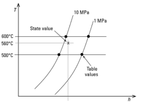
Suppose you take a trip to a power plant and discover that the boiler makes steam at 8 megapascals pressure and 560 degrees Celsius. You can find the enthalpy of the steam from Table A-5 in the appendix. The pressure and temperature aren’t listed in the table, so you have to interpolate both variables. You have to do interpolation three times. To find the enthalpy of the steam $\left(h_1\right)$ at these conditions, follow these steps:
Find the enthalpy of the steam at pressures and temperatures above and below the desired conditions, using Table $A-5$ in the appendix.
$$
\begin{aligned}
& T_{\text {high }}=600^{\circ} \mathrm{C}, P_{\text {ligh }}=10 \mathrm{MPa}, h_{\mathrm{a}}=3,625 \mathrm{~kJ} / \mathrm{kg} \
& T_{\text {high }}=600^{\circ} \mathrm{C}, P_{\text {lou }}=1.0 \mathrm{MPa}, h_b=3,698 \mathrm{~kJ} / \mathrm{kg} \
& T_{\text {law }}=500^{\circ} \mathrm{C}, P_{\text {high }}=10 \mathrm{MPa}, h_c=3,374 \mathrm{~kJ} / \mathrm{kg} \
& T_{\text {low }}=500^{\circ} \mathrm{C}, P_{\text {low }}=1.0 \mathrm{MPa}, h_d=3,478 \mathrm{~kJ} / \mathrm{kg}
\end{aligned}
$$
Figure 3-6 illustrates the pressure, temperature, and enthalpy relationship of this example, showing the locations of the table values relative to the state value of the steam.
Find the enthalpy $h_{\text {wigh }}$ of the steam at $600^{\circ} \mathrm{C}$ and 8 MPa by interpolating the $600^{\circ} \mathrm{C}$ data.
$$
\begin{aligned}
& h_{\text {lijth }}=\frac{(8-1) \mathrm{MPa}}{(10-1) \mathrm{MPa}}\left(h_a-h_b\right)+h_0 \
& h_{\text {tij̣ } 1}=\frac{(8-1) \mathrm{MPa}}{(10-1) \mathrm{MPa}}(3,625-3,698) \mathrm{kJ} / \mathrm{kg}+3,698 \mathrm{~kJ} / \mathrm{kg}=3,641 \mathrm{~kJ} / \mathrm{kg}
\end{aligned}
$$
Find the enthalpy $h_{\text {low }}$ of the steam at $500^{\circ} \mathrm{C}$ and $8 \mathrm{MPa}$ by interpolating the $500^{\circ} \mathrm{C}$ data.
$$
\begin{aligned}
& h_{\mathrm{low}}=\frac{(8-1) \mathrm{MPa}}{(10-1) \mathrm{MPa}}\left(h_c-h_{\mathrm{d}}\right)+h_{\mathrm{d}} \
& h_{\mathrm{low}}=\frac{(8-1) \mathrm{MPa}}{(10-1) \mathrm{MPa}}(3,374-3,478) \mathrm{kJ} / \mathrm{kg}+3,478 \mathrm{~kJ} / \mathrm{kg}=3,397 \mathrm{~kJ} / \mathrm{kg}
\end{aligned}
$$
Find the enthalpy $h_1$ of the steam at $560^{\circ} \mathrm{C}$ and $8 \mathrm{MPa}$ by interpolating the 8 MPa data.
$$
\begin{aligned}
& h_1=\frac{(560-500)^{\circ} \mathrm{C}}{(600-500)^{\circ} \mathrm{C}}\left(h_{\text {tigh }}-h_{\text {tow }}\right)+h_{\mathrm{low}} \
& h_1=\frac{(560-500)^{\circ} \mathrm{C}}{(600-500)^{\circ} \mathrm{C}}(3,641-3,397) \mathrm{kJ} / \mathrm{kg}+3,397 \mathrm{~kJ} / \mathrm{kg}=3,543 \mathrm{~kJ} / \mathrm{kg}
\end{aligned}
$$
热力学代写
代写|热力学代写thermodynamics代考|Figuring out linear interpolation
下面的示例向您展示了如何插入一个表,以查找表中列出的值之间的属性值。你需要知道如何在本书的许多例子中做到这一点,除非你有一个为你计算热力学性质的软件程序。许多热力学教科书都包含一个属性软件包。
可以使用压缩液体的温度和压力来确定比容、内能和焓。例如,根据附录表A-2所示的压缩液态水的热力学性质,可以求出水在22摄氏度和0.1兆帕斯卡压力下的焓。以下步骤向您展示如何通过对附录中的数据进行线性插值来找到焓:
参见附录中的表A-2。
它列出了四种不同的压力:$0.01,0.1,1.0$和$10.0 \mathrm{MPa}$。
为$0.1 \mathrm{MPa}$选择表的部分。
看看$22^{\circ} \mathrm{C}$的温度。
它没有被列出;您必须在$20^{\circ}$和$30^{\circ} \mathrm{C}$之间插入表格。
求焓的值$h_{20}$在$20^{\circ} \mathrm{C}$。
$$
h_{20}=84.03 \mathrm{~kJ} / \mathrm{kg}
$$
求焓的值$h_{30}$在$30^{\circ} \mathrm{C}$。
$$
h_{30}=125.9 \mathrm{~kJ} / \mathrm{kg}
$$
用焓和温度的关系式:
$$
\frac{h_{22}-h_{2 n}}{h_{30}-h_{20}}=\frac{(22-20)^{\circ} \mathrm{C}}{(30-20)^{\circ} \mathrm{C}}
$$
这个方程可以用类似的方法来求热力学能、熵或比容。
物理代写|热力学代写thermodynamics代考|Interpolating with two variables
很多时候,你需要在两个不同的变量之间进行插值,比如温度和压强,才能找到热力学能、焓等性质。两个变量的插值比一个变量的线性插值要棘手一些。下面的示例向您展示了如何使用数据表中的两个变量进行双线性插值。
假设你去了一趟发电厂,发现锅炉在800万帕的压力和560摄氏度的温度下产生蒸汽。你可以从附录的表A-5中找到蒸汽的焓。压强和温度没有列在表中,所以你必须把这两个变量都插进去。你需要做三次插值。要找到这些条件下的蒸汽$\left(h_1\right)$的焓,请遵循以下步骤:
根据附录中的表格$A-5$,求出蒸汽在压力和温度高于或低于所需条件下的焓。
$$
\begin{aligned}
& T_{\text {high }}=600^{\circ} \mathrm{C}, P_{\text {ligh }}=10 \mathrm{MPa}, h_{\mathrm{a}}=3,625 \mathrm{~kJ} / \mathrm{kg} \
& T_{\text {high }}=600^{\circ} \mathrm{C}, P_{\text {lou }}=1.0 \mathrm{MPa}, h_b=3,698 \mathrm{~kJ} / \mathrm{kg} \
& T_{\text {law }}=500^{\circ} \mathrm{C}, P_{\text {high }}=10 \mathrm{MPa}, h_c=3,374 \mathrm{~kJ} / \mathrm{kg} \
& T_{\text {low }}=500^{\circ} \mathrm{C}, P_{\text {low }}=1.0 \mathrm{MPa}, h_d=3,478 \mathrm{~kJ} / \mathrm{kg}
\end{aligned}
$$
图3-6显示了本例的压力、温度和焓的关系,显示了表值相对于蒸汽状态值的位置。
通过插值$600^{\circ} \mathrm{C}$数据,求出$600^{\circ} \mathrm{C}$和8mpa处蒸汽的焓$h_{\text {wigh }}$。
$$
\begin{aligned}
& h_{\text {lijth }}=\frac{(8-1) \mathrm{MPa}}{(10-1) \mathrm{MPa}}\left(h_a-h_b\right)+h_0 \
& h_{\text {tij̣ } 1}=\frac{(8-1) \mathrm{MPa}}{(10-1) \mathrm{MPa}}(3,625-3,698) \mathrm{kJ} / \mathrm{kg}+3,698 \mathrm{~kJ} / \mathrm{kg}=3,641 \mathrm{~kJ} / \mathrm{kg}
\end{aligned}
$$
通过插值$500^{\circ} \mathrm{C}$数据,求出$500^{\circ} \mathrm{C}$和$8 \mathrm{MPa}$处蒸汽的焓$h_{\text {low }}$。
$$
\begin{aligned}
& h_{\mathrm{low}}=\frac{(8-1) \mathrm{MPa}}{(10-1) \mathrm{MPa}}\left(h_c-h_{\mathrm{d}}\right)+h_{\mathrm{d}} \
& h_{\mathrm{low}}=\frac{(8-1) \mathrm{MPa}}{(10-1) \mathrm{MPa}}(3,374-3,478) \mathrm{kJ} / \mathrm{kg}+3,478 \mathrm{~kJ} / \mathrm{kg}=3,397 \mathrm{~kJ} / \mathrm{kg}
\end{aligned}
$$
通过插值8 MPa数据,求出$560^{\circ} \mathrm{C}$和$8 \mathrm{MPa}$处蒸汽的焓$h_1$。
$$
\begin{aligned}
& h_1=\frac{(560-500)^{\circ} \mathrm{C}}{(600-500)^{\circ} \mathrm{C}}\left(h_{\text {tigh }}-h_{\text {tow }}\right)+h_{\mathrm{low}} \
& h_1=\frac{(560-500)^{\circ} \mathrm{C}}{(600-500)^{\circ} \mathrm{C}}(3,641-3,397) \mathrm{kJ} / \mathrm{kg}+3,397 \mathrm{~kJ} / \mathrm{kg}=3,543 \mathrm{~kJ} / \mathrm{kg}
\end{aligned}
$$

统计代写请认准statistics-lab™. statistics-lab™为您的留学生涯保驾护航。
金融工程代写
金融工程是使用数学技术来解决金融问题。金融工程使用计算机科学、统计学、经济学和应用数学领域的工具和知识来解决当前的金融问题,以及设计新的和创新的金融产品。
非参数统计代写
非参数统计指的是一种统计方法,其中不假设数据来自于由少数参数决定的规定模型;这种模型的例子包括正态分布模型和线性回归模型。
广义线性模型代考
广义线性模型(GLM)归属统计学领域,是一种应用灵活的线性回归模型。该模型允许因变量的偏差分布有除了正态分布之外的其它分布。
术语 广义线性模型(GLM)通常是指给定连续和/或分类预测因素的连续响应变量的常规线性回归模型。它包括多元线性回归,以及方差分析和方差分析(仅含固定效应)。
有限元方法代写
有限元方法(FEM)是一种流行的方法,用于数值解决工程和数学建模中出现的微分方程。典型的问题领域包括结构分析、传热、流体流动、质量运输和电磁势等传统领域。
有限元是一种通用的数值方法,用于解决两个或三个空间变量的偏微分方程(即一些边界值问题)。为了解决一个问题,有限元将一个大系统细分为更小、更简单的部分,称为有限元。这是通过在空间维度上的特定空间离散化来实现的,它是通过构建对象的网格来实现的:用于求解的数值域,它有有限数量的点。边界值问题的有限元方法表述最终导致一个代数方程组。该方法在域上对未知函数进行逼近。[1] 然后将模拟这些有限元的简单方程组合成一个更大的方程系统,以模拟整个问题。然后,有限元通过变化微积分使相关的误差函数最小化来逼近一个解决方案。
tatistics-lab作为专业的留学生服务机构,多年来已为美国、英国、加拿大、澳洲等留学热门地的学生提供专业的学术服务,包括但不限于Essay代写,Assignment代写,Dissertation代写,Report代写,小组作业代写,Proposal代写,Paper代写,Presentation代写,计算机作业代写,论文修改和润色,网课代做,exam代考等等。写作范围涵盖高中,本科,研究生等海外留学全阶段,辐射金融,经济学,会计学,审计学,管理学等全球99%专业科目。写作团队既有专业英语母语作者,也有海外名校硕博留学生,每位写作老师都拥有过硬的语言能力,专业的学科背景和学术写作经验。我们承诺100%原创,100%专业,100%准时,100%满意。
随机分析代写
随机微积分是数学的一个分支,对随机过程进行操作。它允许为随机过程的积分定义一个关于随机过程的一致的积分理论。这个领域是由日本数学家伊藤清在第二次世界大战期间创建并开始的。
时间序列分析代写
随机过程,是依赖于参数的一组随机变量的全体,参数通常是时间。 随机变量是随机现象的数量表现,其时间序列是一组按照时间发生先后顺序进行排列的数据点序列。通常一组时间序列的时间间隔为一恒定值(如1秒,5分钟,12小时,7天,1年),因此时间序列可以作为离散时间数据进行分析处理。研究时间序列数据的意义在于现实中,往往需要研究某个事物其随时间发展变化的规律。这就需要通过研究该事物过去发展的历史记录,以得到其自身发展的规律。
回归分析代写
多元回归分析渐进(Multiple Regression Analysis Asymptotics)属于计量经济学领域,主要是一种数学上的统计分析方法,可以分析复杂情况下各影响因素的数学关系,在自然科学、社会和经济学等多个领域内应用广泛。
MATLAB代写
MATLAB 是一种用于技术计算的高性能语言。它将计算、可视化和编程集成在一个易于使用的环境中,其中问题和解决方案以熟悉的数学符号表示。典型用途包括:数学和计算算法开发建模、仿真和原型制作数据分析、探索和可视化科学和工程图形应用程序开发,包括图形用户界面构建MATLAB 是一个交互式系统,其基本数据元素是一个不需要维度的数组。这使您可以解决许多技术计算问题,尤其是那些具有矩阵和向量公式的问题,而只需用 C 或 Fortran 等标量非交互式语言编写程序所需的时间的一小部分。MATLAB 名称代表矩阵实验室。MATLAB 最初的编写目的是提供对由 LINPACK 和 EISPACK 项目开发的矩阵软件的轻松访问,这两个项目共同代表了矩阵计算软件的最新技术。MATLAB 经过多年的发展,得到了许多用户的投入。在大学环境中,它是数学、工程和科学入门和高级课程的标准教学工具。在工业领域,MATLAB 是高效研究、开发和分析的首选工具。MATLAB 具有一系列称为工具箱的特定于应用程序的解决方案。对于大多数 MATLAB 用户来说非常重要,工具箱允许您学习和应用专业技术。工具箱是 MATLAB 函数(M 文件)的综合集合,可扩展 MATLAB 环境以解决特定类别的问题。可用工具箱的领域包括信号处理、控制系统、神经网络、模糊逻辑、小波、仿真等。