如果你也在 怎样代写机器学习machine learning这个学科遇到相关的难题,请随时右上角联系我们的24/7代写客服。
机器学习是一种数据分析的方法,可以自动建立分析模型。它是人工智能的一个分支,其基础是系统可以从数据中学习,识别模式,并在最小的人为干预下做出决定。
statistics-lab™ 为您的留学生涯保驾护航 在代写机器学习machine learning方面已经树立了自己的口碑, 保证靠谱, 高质且原创的统计Statistics代写服务。我们的专家在代写机器学习machine learning方面经验极为丰富,各种代写机器学习machine learning相关的作业也就用不着说。
我们提供的机器学习machine learning及其相关学科的代写,服务范围广, 其中包括但不限于:
- Statistical Inference 统计推断
- Statistical Computing 统计计算
- Advanced Probability Theory 高等楖率论
- Advanced Mathematical Statistics 高等数理统计学
- (Generalized) Linear Models 广义线性模型
- Statistical Machine Learning 统计机器学习
- Longitudinal Data Analysis 纵向数据分析
- Foundations of Data Science 数据科学基础
统计代写|机器学习作业代写machine learning代考|The k-Nearest-Neighbor Rule
How do we establish that a certain object is more similar to $\mathbf{x}$ than to $\mathbf{y}$ ? Some may doubt that this is at all possible. Is giraffe more similar to horse than to zebra? Questions of this kind raise suspicion. Too many arbitrary and subjective factors have to be considered when looking for an answer.
Similarity of Attribute Vectors The machine-learning task formulated in the previous chapters keeps the situation relatively simple. Rather than real objects, the classifier compares their attribute-based descriptions. Thus in the toy domain from Chap. 1, the similarity of two pies can be established by counting the attributes in
which they differ: the fewer the differences, the greater the similarity. The first row in Table $3.1$ gives the attribute values of object $\mathbf{x}$. For each of the twelve training examples that follow, the right-most column specifies the number of differences in the attribute values of the given example and $\mathbf{x}$. The smallest value being found in the case of ex $\mathrm{x}_{5}$, we conclude that this is the training example most similar to $\mathbf{x}$, and $\mathbf{x}$ should thus be labeled with pos, the class of ex 5 .
In Table 3.1, all attributes are discrete, but dealing with continuous attributes is just as easy. Since each example can be represented by a point in an $n$ dimensional space, we can use the Euclidean distance or some other geometric formula (Section $3.2$ will have more to say on this topic); and again, the smaller the distance, the greater the similarity. This, by the way, is how the nearest-neighbor classifier got its name: the training example with the smallest distance from $\mathbf{x}$ in the instance space is, geometrically speaking, $\mathbf{x}$ ‘s nearest neighbor.
统计代写|机器学习作业代写machine learning代考|Measuring Similarity
As mentioned earlier, a natural way to identify the nearest neighbor of some $\mathbf{x}$ is to use the geometrical distances of $\mathbf{x}$ from the training examples. Figure $3.1$ shows a two-dimensional domain where the distances can easily be measured by a rulerbut the ruler surely cannot be used if there are more than three attributes. In that event, we need a mathematical formula.
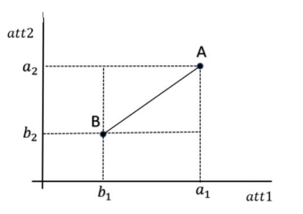
Euclidean Distance In a two-dimensional space, a plane, the geometric distance between two points, $\mathbf{x}=\left(x_{1}, x_{2}\right)$ and $\mathbf{y}=\left(y_{1}, y_{2}\right)$, is measured by the Pythagorean theorem as illustrated in Fig. 3.2: $d(\mathbf{A}, \mathbf{B})=\sqrt{\left(a_{1}-b_{1}\right)^{2}+\left(a_{2}-b_{2}\right)^{2}}$. The following formula generalizes this to $n$-dimensional domains: the Euclidean distance between $\mathbf{x}=\left(x_{1}, \ldots, x_{n}\right)$ and $\mathbf{y}=\left(y_{1}, \ldots, y_{n}\right)$ :
$$
d_{E}(\mathbf{x}, \mathbf{y})=\sqrt{\sum_{i=1}^{n}\left(x_{i}-y_{i}\right)^{2}}
$$
The use of this metric in $k$-NN classifiers is illustrated in Table $3.3$ where the training set consists of four examples described by three numeric attributes.
More General Formulation The reader has noticed that the term under the square root symbol is the sum of the squared distances along the individual attributes. ${ }^{1}$ Mathematically, this is expressed as follows:
$$
d_{M}(\mathbf{x}, \mathbf{y})=\sqrt{\sum_{i=1}^{n} d\left(x_{i}, y_{i}\right)}
$$
统计代写|机器学习作业代写machine learning代考|Irrelevant Attributes and Scaling Problems
The reader now understands the principles of the $k$-NN classifier well enough to be able to write a computer program that implements it. Caution is called for, though. When applied mechanically, the tool may disappoint, and we have to understand why this may happen.
The philosophy underlying this paradigm is telling us that “objects are similar if the geometric distance between the vectors describing them is small.” This said we know that the geometric distance is sometimes misleading. The following two cases are typical.
Irrelevant Attributes It is not true that all attributes are created equal. From the perspective of machine learning, some are irrelevant in the sense that their values have nothing to do with the example’s class-and yet they affect the geometric distance between vectors.
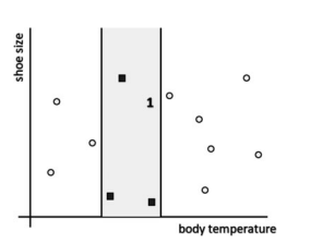
A simple illustration will clarify the point. In the training set from Fig. 3.3, the examples are characterized by two numeric attributes: body-temperature (horizontal axis) and shoe-size (vertical axis). Suppose the $k$-NN classifier is to classify object 1 as healthy (pos) or sick (neg).
All positive examples find themselves in the shaded area delimited by two critical points along the “horizontal” attribute: temperatures exceeding the maximum indicate fever, and those below the minimum indicate hypothermia. As for the “vertical” attribute, though, we see that the positive and negative examples alike are distributed along its entire domain, show-size not being able to affect a person’s health. The object we want to classify is in the highlighted region, and by common sense it should be labeled as positive-despite the fact that its nearest neighbor happens to be negative.
机器学习代写
统计代写|机器学习作业代写machine learning代考|The k-Nearest-Neighbor Rule
我们如何确定某个对象更类似于X比是? 有些人可能怀疑这完全可能。长颈鹿更像马而不是斑马?这类问题引起怀疑。在寻找答案时,必须考虑太多的任意和主观因素。
属性向量的相似性 前面章节中制定的机器学习任务使情况相对简单。分类器不是真实对象,而是比较它们基于属性的描述。因此在第一章的玩具领域。1、两个饼图的相似度可以通过统计其中的属性来确定
它们的不同之处:差异越小,相似性就越大。表中的第一行3.1给出对象的属性值X. 对于随后的 12 个训练示例中的每一个,最右侧的列指定给定示例的属性值的差异数量,以及X. 在 ex 的情况下找到的最小值X5,我们得出结论,这是最相似的训练示例X, 和X因此应该用 pos 标记,即 ex 5 的类别。
在表 3.1 中,所有属性都是离散的,但处理连续属性同样容易。因为每个例子都可以用一个点来表示n维空间,我们可以使用欧几里得距离或其他一些几何公式(第3.2关于这个话题会有更多的发言权);再次,距离越小,相似度越大。顺便说一下,这就是最近邻分类器的名字的由来:距离最小的训练样本X在实例空间中,从几何上讲,X的最近邻居。
统计代写|机器学习作业代写machine learning代考|Measuring Similarity
如前所述,一种识别某些最近邻居的自然方法X是使用几何距离X从训练示例中。数字3.1显示了一个二维域,其中距离可以很容易地用尺子测量,但如果属性超过三个,则肯定不能使用尺子。在那种情况下,我们需要一个数学公式。
欧几里得距离 在二维空间中,一个平面,两点之间的几何距离,X=(X1,X2)和是=(是1,是2), 由勾股定理测量,如图 3.2 所示:d(一种,乙)=(一种1−b1)2+(一种2−b2)2. 下面的公式将其推广到n维域:之间的欧几里得距离X=(X1,…,Xn)和是=(是1,…,是n) :
d和(X,是)=∑一世=1n(X一世−是一世)2
该指标在ķ-NN 分类器如表所示3.3其中训练集由三个数字属性描述的四个示例组成。
更一般的公式读者已经注意到平方根符号下的术语是沿各个属性的平方距离之和。1在数学上,这表示如下:
d米(X,是)=∑一世=1nd(X一世,是一世)
统计代写|机器学习作业代写machine learning代考|Irrelevant Attributes and Scaling Problems
读者现在明白了ķ-NN 分类器足够好,能够编写实现它的计算机程序。不过,需要谨慎。当机械地应用时,该工具可能会令人失望,我们必须了解为什么会发生这种情况。
这种范式背后的哲学告诉我们,“如果描述对象的向量之间的几何距离很小,那么对象就是相似的。” 这就是说我们知道几何距离有时会产生误导。以下两种情况是典型的。
不相关的属性 并非所有属性都是平等的。从机器学习的角度来看,有些是无关紧要的,因为它们的值与示例的类别无关——但它们会影响向量之间的几何距离。
一个简单的插图将阐明这一点。在图 3.3 的训练集中,示例由两个数字属性表征:体温(横轴)和鞋码(纵轴)。假设ķ-NN分类器是将对象1分类为健康(pos)或生病(neg)。
所有正例都位于由“水平”属性的两个临界点界定的阴影区域中:温度超过最大值表示发烧,低于最小值表示体温过低。但是,对于“垂直”属性,我们看到正面和负面的例子都分布在它的整个域上,显示大小不会影响一个人的健康。我们要分类的对象在突出显示的区域中,按照常识,它应该被标记为正数——尽管它最近的邻居恰好是负数。

统计代写请认准statistics-lab™. statistics-lab™为您的留学生涯保驾护航。统计代写|python代写代考
随机过程代考
在概率论概念中,随机过程是随机变量的集合。 若一随机系统的样本点是随机函数,则称此函数为样本函数,这一随机系统全部样本函数的集合是一个随机过程。 实际应用中,样本函数的一般定义在时间域或者空间域。 随机过程的实例如股票和汇率的波动、语音信号、视频信号、体温的变化,随机运动如布朗运动、随机徘徊等等。
贝叶斯方法代考
贝叶斯统计概念及数据分析表示使用概率陈述回答有关未知参数的研究问题以及统计范式。后验分布包括关于参数的先验分布,和基于观测数据提供关于参数的信息似然模型。根据选择的先验分布和似然模型,后验分布可以解析或近似,例如,马尔科夫链蒙特卡罗 (MCMC) 方法之一。贝叶斯统计概念及数据分析使用后验分布来形成模型参数的各种摘要,包括点估计,如后验平均值、中位数、百分位数和称为可信区间的区间估计。此外,所有关于模型参数的统计检验都可以表示为基于估计后验分布的概率报表。
广义线性模型代考
广义线性模型(GLM)归属统计学领域,是一种应用灵活的线性回归模型。该模型允许因变量的偏差分布有除了正态分布之外的其它分布。
statistics-lab作为专业的留学生服务机构,多年来已为美国、英国、加拿大、澳洲等留学热门地的学生提供专业的学术服务,包括但不限于Essay代写,Assignment代写,Dissertation代写,Report代写,小组作业代写,Proposal代写,Paper代写,Presentation代写,计算机作业代写,论文修改和润色,网课代做,exam代考等等。写作范围涵盖高中,本科,研究生等海外留学全阶段,辐射金融,经济学,会计学,审计学,管理学等全球99%专业科目。写作团队既有专业英语母语作者,也有海外名校硕博留学生,每位写作老师都拥有过硬的语言能力,专业的学科背景和学术写作经验。我们承诺100%原创,100%专业,100%准时,100%满意。
机器学习代写
随着AI的大潮到来,Machine Learning逐渐成为一个新的学习热点。同时与传统CS相比,Machine Learning在其他领域也有着广泛的应用,因此这门学科成为不仅折磨CS专业同学的“小恶魔”,也是折磨生物、化学、统计等其他学科留学生的“大魔王”。学习Machine learning的一大绊脚石在于使用语言众多,跨学科范围广,所以学习起来尤其困难。但是不管你在学习Machine Learning时遇到任何难题,StudyGate专业导师团队都能为你轻松解决。
多元统计分析代考
基础数据: $N$ 个样本, $P$ 个变量数的单样本,组成的横列的数据表
变量定性: 分类和顺序;变量定量:数值
数学公式的角度分为: 因变量与自变量
时间序列分析代写
随机过程,是依赖于参数的一组随机变量的全体,参数通常是时间。 随机变量是随机现象的数量表现,其时间序列是一组按照时间发生先后顺序进行排列的数据点序列。通常一组时间序列的时间间隔为一恒定值(如1秒,5分钟,12小时,7天,1年),因此时间序列可以作为离散时间数据进行分析处理。研究时间序列数据的意义在于现实中,往往需要研究某个事物其随时间发展变化的规律。这就需要通过研究该事物过去发展的历史记录,以得到其自身发展的规律。
回归分析代写
多元回归分析渐进(Multiple Regression Analysis Asymptotics)属于计量经济学领域,主要是一种数学上的统计分析方法,可以分析复杂情况下各影响因素的数学关系,在自然科学、社会和经济学等多个领域内应用广泛。
MATLAB代写
MATLAB 是一种用于技术计算的高性能语言。它将计算、可视化和编程集成在一个易于使用的环境中,其中问题和解决方案以熟悉的数学符号表示。典型用途包括:数学和计算算法开发建模、仿真和原型制作数据分析、探索和可视化科学和工程图形应用程序开发,包括图形用户界面构建MATLAB 是一个交互式系统,其基本数据元素是一个不需要维度的数组。这使您可以解决许多技术计算问题,尤其是那些具有矩阵和向量公式的问题,而只需用 C 或 Fortran 等标量非交互式语言编写程序所需的时间的一小部分。MATLAB 名称代表矩阵实验室。MATLAB 最初的编写目的是提供对由 LINPACK 和 EISPACK 项目开发的矩阵软件的轻松访问,这两个项目共同代表了矩阵计算软件的最新技术。MATLAB 经过多年的发展,得到了许多用户的投入。在大学环境中,它是数学、工程和科学入门和高级课程的标准教学工具。在工业领域,MATLAB 是高效研究、开发和分析的首选工具。MATLAB 具有一系列称为工具箱的特定于应用程序的解决方案。对于大多数 MATLAB 用户来说非常重要,工具箱允许您学习和应用专业技术。工具箱是 MATLAB 函数(M 文件)的综合集合,可扩展 MATLAB 环境以解决特定类别的问题。可用工具箱的领域包括信号处理、控制系统、神经网络、模糊逻辑、小波、仿真等。