如果你也在 怎样代写机器学习machine learning这个学科遇到相关的难题，请随时右上角联系我们的24/7代写客服。

机器学习是一种数据分析的方法，可以自动建立分析模型。它是人工智能的一个分支，其基础是系统可以从数据中学习，识别模式，并在最小的人为干预下做出决定。

statistics-lab™ 为您的留学生涯保驾护航 在代写机器学习machine learning方面已经树立了自己的口碑, 保证靠谱, 高质且原创的统计Statistics代写服务。我们的专家在代写机器学习machine learning方面经验极为丰富，各种代写机器学习machine learning相关的作业也就用不着说。

我们提供的机器学习machine learning及其相关学科的代写，服务范围广, 其中包括但不限于:

• Statistical Inference 统计推断
• Statistical Computing 统计计算
• Advanced Probability Theory 高等楖率论
• Advanced Mathematical Statistics 高等数理统计学
• (Generalized) Linear Models 广义线性模型
• Statistical Machine Learning 统计机器学习
• Longitudinal Data Analysis 纵向数据分析
• Foundations of Data Science 数据科学基础

统计代写|机器学习作业代写machine learning代考|Polynomial Classifiers

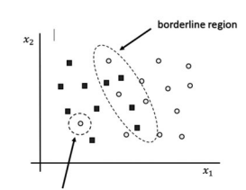
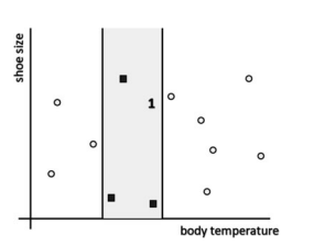
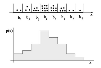
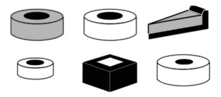
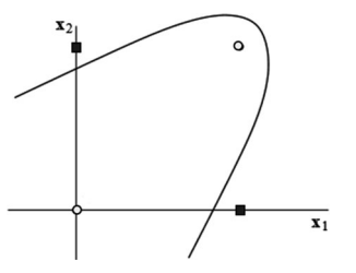
Let us now abandon the strict requirement that positive examples be linearly separable from negative ones. Quite often, they are not. Not only can the linear separability be destroyed by noise; the very shape of the region occupied by one of the classes can render linear decision surface inadequate. Thus in the training set shown in Fig. 4.5, no linear classifier ever succeeds in separating the two squares from the circles. Such separation can only be accomplished by a non-linear curve such as the parabola shown in the picture.

Non-linear Classifiers The point having been made, we have to ask how to induce these non-linear classifiers from data. To begin with, we have to decide what type of function to employ. This is not difficult. Math teaches us that any $n$ dimensional curve can be approximated to arbitrary precision with some polynomial of a sufficiently high order. Let us therefore take a look at how to induce from data these polynomials. Later, we will discuss their practical utility.

Polynomials of the Second Order The good news is that the coefficients of polynomials can be induced by the same techniques that we have used for linear classifiers. Let us explain how.

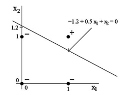
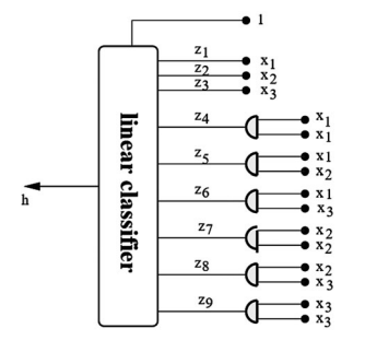
For the sake of clarity, we will begin by constraining ourselves to simple domains with only two Boolean attributes, $x_{1}$ and $x_{2}$. The second-order polynomial is then defined as follows:
$$
w_{0}+w_{1} x_{1}+w_{2} x_{2}+w_{3} x_{1}^{2}+w_{4} x_{1} x_{2}+w_{5} x_{2}^{2}=0
$$
The expression on the left is a sum of terms that have one thing in common: a weight, $w_{i}$, multiplies a product $x_{1}^{k} x_{2}^{l}$. In the first term, we have $k+l=0$, because $w_{0} x_{1}^{0} x_{2}^{0}=w_{0}$; next come the terms with $k+l=1$, concretely, $w_{1} x_{1}^{1} x_{2}^{0}=w_{1} x_{1}$ and $w_{2} x_{1}^{0} x_{2}^{1}=w_{1} x_{2}$; and the sequence ends with three terms that have $k+l=2$ : specifically, $w_{3} x_{1}^{2}, w_{4} x_{1}^{1} x_{2}^{1}$, and $w_{5} x_{2}^{2}$. The thing to remember is that the expansion of the second-order polynomial stops when the sum of the exponents reaches 2 .
Of course, some of the weights can be $w_{i}=0$, rendering the corresponding terms “invisible” such as in $7+2 x_{1} x_{2}+3 x_{2}^{2}$ where the coefficients of $x_{1}, x_{2}$, and $x_{1}^{2}$ are zero.

统计代写|机器学习作业代写machine learning代考|Specific Aspects of Polynomial Classifiers

Now that we understand that the main strength of polynomials is their almost unlimited flexibility, it is time to turn our attention to their shortcomings and limitations.

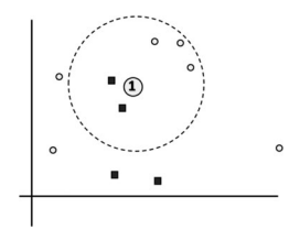
Overfitting Polynomial classifiers tend to overfit noisy training data. Since the problem of overfitting is typical of many machine-learning paradigms, it is a good idea discuss its essence in some detail. Let us constrain ourselves to twodimensional continuous domains that are easy to visualize.

The eight training examples in Fig. $4.7$ fall into two groups. In one group, all examples are positive (empty circles); in the other, all save one are negative (filled circles). Two attempts at separating the two classes are shown. The one on the left uses a linear classifier, ignoring the fact that one training example is thus misclassified. The one on the right resorts to a polynomial classifier in an attempt to avoid any error on the training set.

Inevitable Trade-Off Which of the two is to be preferred? The answer is not straightforward because we do not know the underlying nature of the data. It may be that the two classes are linearly separable, and the only cause for one positive example to be found in the negative region is class-label noise. If this is the case, the single error made by the linear classifier on the training set is inconsequential, whereas the polynomial on the right, cutting deep into the negative area, will misclassify those future examples that find themselves on the wrong side of the

curve. Conversely, it is possible that the outlier does represent some legitimate, even if rare, aspect of the positive class. In this event, the use of the polynomial is justified. Practically speaking, however, the assumption that the single outlier is only noise is more likely to be correct than the “special-aspect” alternative.

A realistic training set will contain not one, but quite a few, perhaps many examples that appear to be in the wrong area of the instance space. And the interclass boundary that the classifier seeks to approximate may indeed be curved, though how much curved is anybody’s guess. The engineer may regard the linear classifier as too crude, and opt instead for the more flexible polynomial. This said, a highorder polynomial will separate the two classes even in a very noisy training set-and then fail miserably on future data. The ideal solution is usually somewhere between the extremes and has to be determined experimentally.

统计代写|机器学习作业代写machine learning代考|Support Vector Machines

Now that we understand that polynomial classifiers do not call for any new learning algorithms, we can return to linear classifiers, a topic we have not yet exhausted. Let us abandon the restriction to the Boolean attributes, and consider also the possibility of the attributes being continuous. Can we then still rely on the two training algorithms described above?

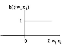
Perceptron Learning in Numeric Domains In the case of perceptron learning, the answer is easy: yes, the same weight-modification formula can be used. Practical experience shows, however, that it is a good idea to normalize all attribute values so that they fall into the unit interval, $x_{i} \in[0,1]$. We can use to this end the normalization technique described in the chapter dealing with nearest-neighbor classifiers, in Sect. 3.3.
Let us repeat, for the reader’s convenience, the weight-adjusting formula:
$$
w_{i}=w_{i}+\eta[c(\mathbf{x})-h(\mathbf{x})] x_{i}
$$
Learning rate, $\eta$, and the difference between the real and hypothesized class labels, $[c(\mathbf{x})-h(\mathbf{x})]$, have the same meaning and impact as before. What has changed is the role of $x_{i}$. In the case of Boolean attributes, the value of $x_{i}=1$ or $x_{i}=0$ decided whether or not the corresponding weight should change. Here, however, the value of $x_{i}$ decides how much the weight should be affected: the change is greater if the attribute’s value is higher.

机器学习代写

统计代写|机器学习作业代写machine learning代考|Polynomial Classifiers

现在让我们放弃正样本与负样本线性可分的严格要求。很多时候，他们不是。不仅线性可分性会被噪声破坏；其中一类所占据的区域的形状可能会导致线性决策面不足。因此，在图 4.5 所示的训练集中，没有任何线性分类器能够成功地将两个正方形与圆形分开。这种分离只能通过非线性曲线来完成，例如图中所示的抛物线。

非线性分类器 已经提出了这一点，我们必须问如何从数据中归纳出这些非线性分类器。首先，我们必须决定使用什么类型的函数。这并不难。数学告诉我们，任何n尺寸曲线可以用一些足够高阶的多项式逼近到任意精度。因此，让我们看看如何从数据中导出这些多项式。稍后，我们将讨论它们的实际用途。

二阶多项式 好消息是多项式的系数可以通过我们用于线性分类器的相同技术来导出。让我们解释一下。

为了清楚起见，我们首先将自己限制在只有两个布尔属性的简单域中，X1和X2. 然后将二阶多项式定义如下：
在0+在1X1+在2X2+在3X12+在4X1X2+在5X22=0
左边的表达式是具有一个共同点的项的总和：权重，在一世, 乘积X1ķX2l. 在第一学期，我们有ķ+l=0， 因为在0X10X20=在0; 接下来是条款ķ+l=1, 具体来说,在1X11X20=在1X1和在2X10X21=在1X2; 并且该序列以三个具有的项结束ķ+l=2： 具体来说，在3X12,在4X11X21， 和在5X22. 要记住的是，当指数之和达到 2 时，二阶多项式的展开将停止。
当然，有些权重可以在一世=0，使相应的术语“不可见”，例如7+2X1X2+3X22其中的系数X1,X2， 和X12为零。

统计代写|机器学习作业代写machine learning代考|Specific Aspects of Polynomial Classifiers

既然我们了解多项式的主要优势在于它们几乎无限的灵活性，那么是时候将注意力转向它们的缺点和局限性了。

过拟合多项式分类器倾向于过拟合嘈杂的训练数据。由于过度拟合问题是许多机器学习范式的典型问题，因此最好详细讨论其本质。让我们将自己限制在易于可视化的二维连续域中。

图 8 中的 8 个训练样例。4.7分为两组。在一组中，所有示例都是正面的（空心圆圈）；另一方面，除了一个都是负数（实心圆圈）。显示了分离这两个类的两次尝试。左边的那个使用线性分类器，忽略了一个训练示例因此被错误分类的事实。右边的那个求助于多项式分类器，试图避免训练集上的任何错误。

不可避免的权衡 两者中的哪一个是首选？答案并不简单，因为我们不知道数据的基本性质。可能这两个类是线性可分的，在负区域中找到一个正样本的唯一原因是类标签噪声。如果是这种情况，线性分类器在训练集上产生的单个错误是无关紧要的，而右边的多项式深入到负区域，将错误分类那些发现自己在错误一侧的未来示例

曲线。相反，异常值可能确实代表了正类的一些合法的，即使是罕见的方面。在这种情况下，使用多项式是合理的。然而，实际上，单个异常值只是噪声的假设比“特殊方面”替代方案更可能是正确的。

一个真实的训练集不会包含一个，而是相当多，也许很多的例子似乎在实例空间的错误区域。并且分类器试图近似的类间边界可能确实是弯曲的，尽管任何人都猜测弯曲的程度。工程师可能认为线性分类器过于粗糙，而选择更灵活的多项式。这就是说，即使在非常嘈杂的训练集中，高阶多项式也会将这两个类分开——然后在未来的数据上惨遭失败。理想的解决方案通常介于两个极端之间，并且必须通过实验确定。

统计代写|机器学习作业代写machine learning代考|Support Vector Machines

现在我们知道多项式分类器不需要任何新的学习算法，我们可以回到线性分类器，这是一个我们还没有穷尽的话题。让我们放弃对布尔属性的限制，同时考虑属性连续的可能性。那么我们还可以依赖上面描述的两种训练算法吗？

数值域中的感知器学习在感知器学习的情况下，答案很简单：是的，可以使用相同的权重修正公式。然而，实践经验表明，将所有属性值归一化以使其落入单位区间是一个好主意，X一世∈[0,1]. 为此，我们可以使用第 3 节中处理最近邻分类器一章中描述的规范化技术。3.3.
为方便读者，让我们重复一下权重调整公式：
在一世=在一世+这[C(X)−H(X)]X一世
学习率，这，以及真实和假设的类标签之间的差异，[C(X)−H(X)], 与以前的含义和影响相同。改变的是角色X一世. 在布尔属性的情况下，值X一世=1或者X一世=0决定相应的权重是否应该改变。然而，这里的价值X一世决定权重应该受到多大的影响：如果属性的值越高，变化越大。

统计代写请认准statistics-lab™. statistics-lab™为您的留学生涯保驾护航。统计代写|python代写代考

随机过程代考

在概率论概念中，随机过程是随机变量的集合。 若一随机系统的样本点是随机函数，则称此函数为样本函数，这一随机系统全部样本函数的集合是一个随机过程。 实际应用中，样本函数的一般定义在时间域或者空间域。 随机过程的实例如股票和汇率的波动、语音信号、视频信号、体温的变化，随机运动如布朗运动、随机徘徊等等。

贝叶斯方法代考

贝叶斯统计概念及数据分析表示使用概率陈述回答有关未知参数的研究问题以及统计范式。后验分布包括关于参数的先验分布，和基于观测数据提供关于参数的信息似然模型。根据选择的先验分布和似然模型，后验分布可以解析或近似，例如，马尔科夫链蒙特卡罗 (MCMC) 方法之一。贝叶斯统计概念及数据分析使用后验分布来形成模型参数的各种摘要，包括点估计，如后验平均值、中位数、百分位数和称为可信区间的区间估计。此外，所有关于模型参数的统计检验都可以表示为基于估计后验分布的概率报表。

广义线性模型代考

广义线性模型（GLM）归属统计学领域，是一种应用灵活的线性回归模型。该模型允许因变量的偏差分布有除了正态分布之外的其它分布。

statistics-lab作为专业的留学生服务机构，多年来已为美国、英国、加拿大、澳洲等留学热门地的学生提供专业的学术服务，包括但不限于Essay代写，Assignment代写，Dissertation代写，Report代写，小组作业代写，Proposal代写，Paper代写，Presentation代写，计算机作业代写，论文修改和润色，网课代做，exam代考等等。写作范围涵盖高中，本科，研究生等海外留学全阶段，辐射金融，经济学，会计学，审计学，管理学等全球99%专业科目。写作团队既有专业英语母语作者，也有海外名校硕博留学生，每位写作老师都拥有过硬的语言能力，专业的学科背景和学术写作经验。我们承诺100%原创，100%专业，100%准时，100%满意。

机器学习代写

随着AI的大潮到来，Machine Learning逐渐成为一个新的学习热点。同时与传统CS相比，Machine Learning在其他领域也有着广泛的应用，因此这门学科成为不仅折磨CS专业同学的“小恶魔”，也是折磨生物、化学、统计等其他学科留学生的“大魔王”。学习Machine learning的一大绊脚石在于使用语言众多，跨学科范围广，所以学习起来尤其困难。但是不管你在学习Machine Learning时遇到任何难题，StudyGate专业导师团队都能为你轻松解决。

多元统计分析代考

基础数据: $N$ 个样本， $P$ 个变量数的单样本，组成的横列的数据表
变量定性: 分类和顺序；变量定量：数值
数学公式的角度分为: 因变量与自变量

时间序列分析代写

随机过程，是依赖于参数的一组随机变量的全体，参数通常是时间。 随机变量是随机现象的数量表现，其时间序列是一组按照时间发生先后顺序进行排列的数据点序列。通常一组时间序列的时间间隔为一恒定值（如1秒，5分钟，12小时，7天，1年），因此时间序列可以作为离散时间数据进行分析处理。研究时间序列数据的意义在于现实中，往往需要研究某个事物其随时间发展变化的规律。这就需要通过研究该事物过去发展的历史记录，以得到其自身发展的规律。

回归分析代写

多元回归分析渐进（Multiple Regression Analysis Asymptotics）属于计量经济学领域，主要是一种数学上的统计分析方法，可以分析复杂情况下各影响因素的数学关系，在自然科学、社会和经济学等多个领域内应用广泛。

MATLAB代写

MATLAB 是一种用于技术计算的高性能语言。它将计算、可视化和编程集成在一个易于使用的环境中，其中问题和解决方案以熟悉的数学符号表示。典型用途包括：数学和计算算法开发建模、仿真和原型制作数据分析、探索和可视化科学和工程图形应用程序开发，包括图形用户界面构建MATLAB 是一个交互式系统，其基本数据元素是一个不需要维度的数组。这使您可以解决许多技术计算问题，尤其是那些具有矩阵和向量公式的问题，而只需用 C 或 Fortran 等标量非交互式语言编写程序所需的时间的一小部分。MATLAB 名称代表矩阵实验室。MATLAB 最初的编写目的是提供对由 LINPACK 和 EISPACK 项目开发的矩阵软件的轻松访问，这两个项目共同代表了矩阵计算软件的最新技术。MATLAB 经过多年的发展，得到了许多用户的投入。在大学环境中，它是数学、工程和科学入门和高级课程的标准教学工具。在工业领域，MATLAB 是高效研究、开发和分析的首选工具。MATLAB 具有一系列称为工具箱的特定于应用程序的解决方案。对于大多数 MATLAB 用户来说非常重要，工具箱允许您学习和应用专业技术。工具箱是 MATLAB 函数（M 文件）的综合集合，可扩展 MATLAB 环境以解决特定类别的问题。可用工具箱的领域包括信号处理、控制系统、神经网络、模糊逻辑、小波、仿真等。

R语言代写	问卷设计与分析代写
PYTHON代写	回归分析与线性模型代写
MATLAB代写	方差分析与试验设计代写
STATA代写	机器学习/统计学习代写
SPSS代写	计量经济学代写
EVIEWS代写	时间序列分析代写
EXCEL代写	深度学习代写
SQL代写	各种数据建模与可视化代写

如果你也在 怎样代写机器学习machine learning这个学科遇到相关的难题，请随时右上角联系我们的24/7代写客服。

机器学习是一种数据分析的方法，可以自动建立分析模型。它是人工智能的一个分支，其基础是系统可以从数据中学习，识别模式，并在最小的人为干预下做出决定。

statistics-lab™ 为您的留学生涯保驾护航 在代写机器学习machine learning方面已经树立了自己的口碑, 保证靠谱, 高质且原创的统计Statistics代写服务。我们的专家在代写机器学习machine learning方面经验极为丰富，各种代写机器学习machine learning相关的作业也就用不着说。

我们提供的机器学习machine learning及其相关学科的代写，服务范围广, 其中包括但不限于:

• Statistical Inference 统计推断
• Statistical Computing 统计计算
• Advanced Probability Theory 高等楖率论
• Advanced Mathematical Statistics 高等数理统计学
• (Generalized) Linear Models 广义线性模型
• Statistical Machine Learning 统计机器学习
• Longitudinal Data Analysis 纵向数据分析
• Foundations of Data Science 数据科学基础

统计代写|机器学习作业代写machine learning代考|Essence

To begin, let us constrain ourselves to Boolean domains where each attribute is either true or false. To be able to use these attributes in algebraic functions, we will represent them by integers: true by 1 , and false by 0 .

Linear Classifier In Fig. 4.1, one example is labeled as positive and the remaining three as negative. In this particular case, the two classes are separated by the linear function defined as follows:

In the expression on the left-hand side, $x_{1}$ and $x_{2}$ represent attributes. If we substitute for $x_{1}$ and $x_{2}$ the concrete values of a given example $(0$ or 1$)$, the expression $-1.2+0.5 x_{1}+x_{2}$ will be either positive or negative. The sign then determines the example’s class. The table on the right shows how the four examples from the left are thus classified.

Equation $4.1$ is not the only one capable of doing the job. Other expressions, say, $-1.5+x_{1}+x_{2}$, will label the four examples in exactly the same way. As a matter of fact, the same can be accomplished by infinitely many classifiers of the following generic form:
$$
w_{0}+w_{1} x_{1}+w_{2} x_{2}=0
$$
The function is easy to generalize to domains with $n$ attributes:
$$
w_{0}+w_{1} x_{1}+\ldots+w_{n} x_{n}=0
$$
If $n=2$, Eq. $4.2$ defines a line; if $n=3$, a plane; and if $n>3$, a hyperplane. If we introduce a “zeroth” attribute, $x_{0}$, that is not used in example description and whose value is always fixed at $x_{0}=1$, the equation can be re-written in the following compact form:
$$
\sum_{i=0}^{n} w_{i} x_{i}=0
$$

统计代写|机器学习作业代写machine learning代考|Perceptron Learning

Having developed some basic understanding of how the linear classifier works, we are ready to take a look at how to induce it from training data.

Learning Task Let us assume that each training example, $\mathbf{x}$, is described by $n$ binary attributes whose values are either $x_{i}=1$ or $x_{i}=0$. A positive example is indicated by $c(\mathbf{x})=1$, and a negative by $c(\mathbf{x})=0$. To make sure we do not confuse the example’s real class with the one suggested by the classifier, we will denote the latter by $h(\mathbf{x})$ where the letter $h$ emphasizes that this is the classifier’s hypothesis. If $\sum_{i=0}^{n} w_{i} x_{i}>0$, the classifier “hypothesizes” that the example is positive and therefore returns $h(\mathbf{x})=1$. Conversely, if $\sum_{i=0}^{n} w_{i} x_{i} \leq 0$, the classifier returns $h(\mathbf{x})=0$. Figure $4.2$ reminds us that the classifier labels $\mathbf{x}$ as positive only if the cumulative evidence supporting this class exceeds 0 .

Finally, we will assume that examples with $c(\mathbf{x})=1$ are linearly separable from those with $c(\mathbf{x})=0$. This means that there exists a linear classifier that will label correctly all training examples so that $h(\mathbf{x})=c(\mathbf{x})$ for any $\mathbf{x}$. The task for machine learning is to find the weights, $w_{i}$, that make this happen.

Learning from Mistakes Here is the essence of the most common approach to induction of linear classifiers. Suppose we have a working version of the classifier, even if imperfect. When presented with a training example, $\mathbf{x}$, the classifier suggests a label, $h(\mathbf{x})$. If this differs from the true class, $h(\mathbf{x}) \neq c(\mathbf{x})$, the learner concludes that the weights should be modified in a way likely to correct this error.

Let the true class be $c(\mathbf{x})=1$. In this event, $h(\mathbf{x})=0$ will only happen if $\sum_{i=0}^{n} w_{i} x_{i}<0$, an indication that the weights are too small. If we increase them, the sum, $\sum_{i=0}^{n} w_{i} x_{i}$, may exceed zero, making the returned label positive, and therefore correct. Note that it is enough to increase only the weights of attributes with $x_{i}=1$; when $x_{i}=0$, then the value of $w_{i}$ does not matter because anything multiplied by zero is still zero: $0 \cdot w_{i}=0$.

Likewise, if $c(\mathbf{x})=0$ and $h(\mathbf{x})=1$, then the weights of all attributes with $x_{i}=1$ should be decreased so as to give the sum the chance to drop below zero, $\sum_{i=0}^{n} w_{i} x_{i}<0$, in which case the classifier will label $\mathbf{x}$ as negative.

统计代写|机器学习作业代写machine learning代考|Domains with More Than Two Classes

Having only two sides, a hyper-plane may separate the positive examples from the negative examples-and that is all. When it comes to multi-class domains, the tool seems helpless. Or is it?

Groups of Binary Classifiers What exceeds the powers of an individual can be solved by a team. One practical solution is shown in Fig. 4.4. The “team” consists of four binary classifiers, each specializing on one of the four classes, $C_{1}$ through $C_{4}$. Ideally, the presentation of an example from $C_{i}$ results in the $i$-th classifier returning $h_{i}(\mathbf{x})=1$, and all the other classifiers returning $h_{j}(\mathbf{x})=0$, assuming, again, that each class is linearly separable from the other classes.

Modifying the Training Data To exhibit this behavior, the individual classifiers need to be properly trained. This training can be accomplished by any of the two algorithms from the previous sections. The only additional trick is that the engineer needs to modify the training data.

Table $4.5$ illustrates the principle. On the left is the original training set, $T$, where each example is labeled with one of the four classes. On the right are four “derived” sets, $T_{1}$ through $T_{4}$, each consisting of the same six examples which have now been re-labeled so that an example that in the original set, $T$, represents class $C_{i}$ is labeled with $c(\mathbf{x})=1$ in $T_{i}$ and with $c(\mathbf{x})=0$ in all other sets.

Needing a Master Classifier The training sets, $T_{i}$, are presented to a program that induces from each of them a linear classifier dedicated to the corresponding class. This is not the end of the story, though. The training examples may poorly represent the classes, they may be corrupted by noise, and even the requirement of linear separability may be violated. As a result, the induced classifiers may overlap each other in the sense that two or more of them will respond to the same example, $\mathbf{x}$, with $h_{i}(\mathbf{x})=1$, leaving the incorrect impression that $\mathbf{x}$ simultaneously belongs to more than one class. This is why a master classifier is needed; its task is to choose from the returned classes the one most likely to be correct.

机器学习代写

统计代写|机器学习作业代写machine learning代考|Essence

首先，让我们将自己限制在每个属性为真或假的布尔域中。为了能够在代数函数中使用这些属性，我们将用整数表示它们：true 用 1 表示，false 用 0 表示。

线性分类器 在图 4.1 中，一个例子被标记为正例，其余三个被标记为负例。在这种特殊情况下，两个类由定义如下的线性函数分开：

在左侧的表达式中，X1和X2表示属性。如果我们替换X1和X2给定示例的具体值(0或 1)， 表达方式−1.2+0.5X1+X2将是积极的或消极的。然后该符号确定示例的类别。右侧的表格显示了如何对左侧的四个示例进行分类。

方程4.1不是唯一有能力做这项工作的人。其他表达方式，例如，−1.5+X1+X2, 将以完全相同的方式标记四个示例。事实上，同样可以通过以下通用形式的无限多个分类器来完成：
在0+在1X1+在2X2=0
该函数很容易推广到具有n属性：
在0+在1X1+…+在nXn=0
如果n=2, 方程。4.2定义一条线；如果n=3， 一架飞机; 而如果n>3，一个超平面。如果我们引入一个“零”属性，X0，在示例描述中未使用，其值始终固定为X0=1，方程可以重写为以下紧凑形式：
∑一世=0n在一世X一世=0

统计代写|机器学习作业代写machine learning代考|Perceptron Learning

在对线性分类器的工作原理有了一些基本的了解之后，我们准备看看如何从训练数据中诱导它。

学习任务让我们假设每个训练示例，X, 描述为n二进制属性，其值为X一世=1或者X一世=0. 一个积极的例子是C(X)=1, 和否定的C(X)=0. 为了确保我们不会将示例的真实类与分类器建议的类混淆，我们将后者表示为H(X)信在哪里H强调这是分类器的假设。如果∑一世=0n在一世X一世>0，分类器“假设”这个例子是正的，因此返回H(X)=1. 相反，如果∑一世=0n在一世X一世≤0，分类器返回H(X)=0. 数字4.2提醒我们分类器标签X仅当支持此类的累积证据超过 0 时才为正。

最后，我们将假设示例C(X)=1与那些线性可分的C(X)=0. 这意味着存在一个线性分类器，它将正确标记所有训练示例，以便H(X)=C(X)对于任何X. 机器学习的任务是找到权重，在一世，这使得这发生。

从错误中学习这是最常见的线性分类器归纳方法的本质。假设我们有一个分类器的工作版本，即使不完美。当呈现一个训练示例时，X，分类器建议一个标签，H(X). 如果这与真正的课程不同，H(X)≠C(X)，学习者得出结论，应该以可能纠正此错误的方式修改权重。

让真正的班级成为C(X)=1. 在本次活动中，H(X)=0只有当∑一世=0n在一世X一世<0，表明权重太小。如果我们增加它们，总和，∑一世=0n在一世X一世, 可能超过零，使返回的标签为正，因此是正确的。请注意，仅增加属性的权重就足够了X一世=1; 什么时候X一世=0，那么值在一世没关系，因为任何乘以零仍然为零：0⋅在一世=0.

同样，如果C(X)=0和H(X)=1, 那么所有属性的权重为X一世=1应减少以使总和有机会降至零以下，∑一世=0n在一世X一世<0, 在这种情况下分类器将标记X为阴性。

统计代写|机器学习作业代写machine learning代考|Domains with More Than Two Classes

只有两条边的超平面可以将正样本与负样本分开——仅此而已。当涉及到多类域时，该工具似乎束手无策。或者是吗？

二元分类器组 超出个人能力的问题可以由团队解决。一种实用的解决方案如图 4.4 所示。“团队”由四个二元分类器组成，每个分类器专门处理四个类中的一个，C1通过C4. 理想情况下，展示一个来自C一世结果是一世-th 分类器返回H一世(X)=1，以及所有其他分类器返回Hj(X)=0，再次假设每个类与其他类是线性可分的。

修改训练数据 为了表现出这种行为，需要对各个分类器进行适当的训练。这种训练可以通过前几节中的两种算法中的任何一种来完成。唯一的额外技巧是工程师需要修改训练数据。

桌子4.5说明原理。左边是原始训练集，吨，其中每个示例都标有四个类别之一。右边是四个“派生”集，吨1通过吨4，每个都由相同的六个示例组成，这些示例现在已重新标记，因此原始集合中的示例，吨, 代表类C一世标有C(X)=1在吨一世与C(X)=0在所有其他集合中。

需要一个主分类器训练集，吨一世, 被呈现给一个程序，该程序从它们中的每一个中引入一个专用于相应类的线性分类器。不过，这还不是故事的结局。训练样本可能无法很好地代表类，它们可能会被噪声破坏，甚至可能违反线性可分性的要求。结果，诱导分类器可能会相互重叠，因为它们中的两个或多个将响应同一个示例，X， 和H一世(X)=1, 留下不正确的印象X同时属于多个类别。这就是需要主分类器的原因；它的任务是从返回的类中选择最有可能是正确的类。

统计代写请认准statistics-lab™. statistics-lab™为您的留学生涯保驾护航。统计代写|python代写代考

随机过程代考

在概率论概念中，随机过程是随机变量的集合。 若一随机系统的样本点是随机函数，则称此函数为样本函数，这一随机系统全部样本函数的集合是一个随机过程。 实际应用中，样本函数的一般定义在时间域或者空间域。 随机过程的实例如股票和汇率的波动、语音信号、视频信号、体温的变化，随机运动如布朗运动、随机徘徊等等。

贝叶斯方法代考

贝叶斯统计概念及数据分析表示使用概率陈述回答有关未知参数的研究问题以及统计范式。后验分布包括关于参数的先验分布，和基于观测数据提供关于参数的信息似然模型。根据选择的先验分布和似然模型，后验分布可以解析或近似，例如，马尔科夫链蒙特卡罗 (MCMC) 方法之一。贝叶斯统计概念及数据分析使用后验分布来形成模型参数的各种摘要，包括点估计，如后验平均值、中位数、百分位数和称为可信区间的区间估计。此外，所有关于模型参数的统计检验都可以表示为基于估计后验分布的概率报表。

广义线性模型代考

广义线性模型（GLM）归属统计学领域，是一种应用灵活的线性回归模型。该模型允许因变量的偏差分布有除了正态分布之外的其它分布。

statistics-lab作为专业的留学生服务机构，多年来已为美国、英国、加拿大、澳洲等留学热门地的学生提供专业的学术服务，包括但不限于Essay代写，Assignment代写，Dissertation代写，Report代写，小组作业代写，Proposal代写，Paper代写，Presentation代写，计算机作业代写，论文修改和润色，网课代做，exam代考等等。写作范围涵盖高中，本科，研究生等海外留学全阶段，辐射金融，经济学，会计学，审计学，管理学等全球99%专业科目。写作团队既有专业英语母语作者，也有海外名校硕博留学生，每位写作老师都拥有过硬的语言能力，专业的学科背景和学术写作经验。我们承诺100%原创，100%专业，100%准时，100%满意。

机器学习代写

随着AI的大潮到来，Machine Learning逐渐成为一个新的学习热点。同时与传统CS相比，Machine Learning在其他领域也有着广泛的应用，因此这门学科成为不仅折磨CS专业同学的“小恶魔”，也是折磨生物、化学、统计等其他学科留学生的“大魔王”。学习Machine learning的一大绊脚石在于使用语言众多，跨学科范围广，所以学习起来尤其困难。但是不管你在学习Machine Learning时遇到任何难题，StudyGate专业导师团队都能为你轻松解决。

多元统计分析代考

基础数据: $N$ 个样本， $P$ 个变量数的单样本，组成的横列的数据表
变量定性: 分类和顺序；变量定量：数值
数学公式的角度分为: 因变量与自变量

时间序列分析代写

随机过程，是依赖于参数的一组随机变量的全体，参数通常是时间。 随机变量是随机现象的数量表现，其时间序列是一组按照时间发生先后顺序进行排列的数据点序列。通常一组时间序列的时间间隔为一恒定值（如1秒，5分钟，12小时，7天，1年），因此时间序列可以作为离散时间数据进行分析处理。研究时间序列数据的意义在于现实中，往往需要研究某个事物其随时间发展变化的规律。这就需要通过研究该事物过去发展的历史记录，以得到其自身发展的规律。

回归分析代写

多元回归分析渐进（Multiple Regression Analysis Asymptotics）属于计量经济学领域，主要是一种数学上的统计分析方法，可以分析复杂情况下各影响因素的数学关系，在自然科学、社会和经济学等多个领域内应用广泛。

MATLAB代写

MATLAB 是一种用于技术计算的高性能语言。它将计算、可视化和编程集成在一个易于使用的环境中，其中问题和解决方案以熟悉的数学符号表示。典型用途包括：数学和计算算法开发建模、仿真和原型制作数据分析、探索和可视化科学和工程图形应用程序开发，包括图形用户界面构建MATLAB 是一个交互式系统，其基本数据元素是一个不需要维度的数组。这使您可以解决许多技术计算问题，尤其是那些具有矩阵和向量公式的问题，而只需用 C 或 Fortran 等标量非交互式语言编写程序所需的时间的一小部分。MATLAB 名称代表矩阵实验室。MATLAB 最初的编写目的是提供对由 LINPACK 和 EISPACK 项目开发的矩阵软件的轻松访问，这两个项目共同代表了矩阵计算软件的最新技术。MATLAB 经过多年的发展，得到了许多用户的投入。在大学环境中，它是数学、工程和科学入门和高级课程的标准教学工具。在工业领域，MATLAB 是高效研究、开发和分析的首选工具。MATLAB 具有一系列称为工具箱的特定于应用程序的解决方案。对于大多数 MATLAB 用户来说非常重要，工具箱允许您学习和应用专业技术。工具箱是 MATLAB 函数（M 文件）的综合集合，可扩展 MATLAB 环境以解决特定类别的问题。可用工具箱的领域包括信号处理、控制系统、神经网络、模糊逻辑、小波、仿真等。

R语言代写	问卷设计与分析代写
PYTHON代写	回归分析与线性模型代写
MATLAB代写	方差分析与试验设计代写
STATA代写	机器学习/统计学习代写
SPSS代写	计量经济学代写
EVIEWS代写	时间序列分析代写
EXCEL代写	深度学习代写
SQL代写	各种数据建模与可视化代写

如果你也在 怎样代写机器学习machine learning这个学科遇到相关的难题，请随时右上角联系我们的24/7代写客服。

机器学习是一种数据分析的方法，可以自动建立分析模型。它是人工智能的一个分支，其基础是系统可以从数据中学习，识别模式，并在最小的人为干预下做出决定。

statistics-lab™ 为您的留学生涯保驾护航 在代写机器学习machine learning方面已经树立了自己的口碑, 保证靠谱, 高质且原创的统计Statistics代写服务。我们的专家在代写机器学习machine learning方面经验极为丰富，各种代写机器学习machine learning相关的作业也就用不着说。

我们提供的机器学习machine learning及其相关学科的代写，服务范围广, 其中包括但不限于:

• Statistical Inference 统计推断
• Statistical Computing 统计计算
• Advanced Probability Theory 高等楖率论
• Advanced Mathematical Statistics 高等数理统计学
• (Generalized) Linear Models 广义线性模型
• Statistical Machine Learning 统计机器学习
• Longitudinal Data Analysis 纵向数据分析
• Foundations of Data Science 数据科学基础

统计代写|机器学习作业代写machine learning代考|Removing Redundant Examples

Some training examples do not hurt classification, and yet we want to get rid of them because they are redundant: they add to computational costs without affecting the classifier’s classification performance.

Redundant Examples and Computational Costs In machine-learning practice, we may encounter domains with $10^{6}$ training examples described by some $10^{4}$ attributes. Moreover, one may need to classify thousands of objects as quickly as possible. To identify the nearest neighbor of a single object, the nearest classifier relying on Euclidean distance has to carry out $10^{6} \times 10^{4}=10^{10}$ arithmetic operations. Repeating this for thousands of objects results in $10^{10} \times 10^{3}=10^{13}$ arithmetic operations. This may be impractical.

Fortunately, training sets are often redundant in the sense that the $k=\mathrm{NN}$ classifier’s behavior will be unaffected by the deletion of many training examples. Sometimes, a great majority of the examples can thus be removed with impunity. This is the case of the domain shown in the upper-left corner of Fig. 3.9.

Consistent Subset Redundancy is reduced if we replace the training set, $T$, with its consistent subset, $S$. In the machine-learning context, $S$ is said to be a consistent subset of $T$ if replacing $T$ with $S$ does not affect the class labels returned by the $k$ NN classifier. This definition, however, is not very practical because we do not know how the $k$-NN classifier (whether using $T$ or $S$ ) will behave on future examples. Let

us therefore modify the criterion: $S$ will be regarded as a consistent subset of $T$ if any ex $\in T$ receives the same label from the classifier, no matter whether the $k$-NN classifier is applied to $T-{\mathbf{e x}}$ or to $S-{\mathbf{e x}}$.

Quite often, a realistic training set has many consistent subsets. How do we choose the best one? Intuitively, the smaller the subset, the better. But a perfectionist who insists on having the smallest consistent subset may come to grief because such ideal can usually be achieved only at the price of enormous computational costs. The practically minded engineer who does not believe exorbitant costs are justified will welcome a computationally efficient algorithm that “reasonably downsizes” the original set, unscientific though such formulation may appear to be.

Creating a Consistent Subset One such pragmatic technique is presented in Table 3.6. The algorithm starts by placing one random example from each class in set $S$. This set, $S$, is then used by the l-NN classifier to decide about the labels of all training examples. At this stage, it is likely that some training examples will thus be misclassified. These misclassified examples are added to $S$, and the whole procedure is repeated using this larger version of $S$. The procedure is then repeated all over again. At a certain moment, $S$ becomes sufficiently representative to allow the 1 -NN classifier to label all training examples correctly.

统计代写|机器学习作业代写machine learning代考|Limitations of Attribute-Vector Similarity

The successful practitioner of machine learning has to have a good understanding of the limitations of the diverse tools. Here are some ideas concerning classification based on geometric distances between attribute vectors.

Common Perception of Kangaroos Any child will tell you that a kangaroo is easily recognized by the poach on its belly. Among all the attributes describing the examples, the Boolean information about the presence or the absence of the “pocket” is the most prominent, and it is not an exaggeration to claim that its importance is greater than that of all the remaining attributes combined. Giraffe does not have it, nor does a mosquito or an earthworm.

One Limitation of Attribute Vectors Dividing attributes into relevant, irrelevant, and redundant is too crude. The “kangaroo” experience shows us that among the relevant ones, some are more important than others; a circumstance is not easily reflected in similarity measures, at least not in those discussed in this chapter.

Ideally, $k$-NN should perhaps weigh the relative importance of the individual attributes and adjust the similarity measures accordingly. This is rarely done, in this paradigm. In the next chapter, we will see that this requirement is more naturally addressed by linear classifiers.

Relations Between Attributes Another clearly observable feature in kangaroos is that their front legs are much shorter than the hind legs. This feature, however, is not immediately reflected by similarities derived from geometric distances between attribute vectors. Typically, examples of animals will be described by such attributes as the length of a front leg and the length of a hind leg (among many others), but relation between the different lengths is only implicit.

The reader will now agree that the classification may depend less on the original attributes than on the relations between individual attributes, such as $a_{1} / a_{2}$. One step further, a complex function of two or more attributes will be more informative than the individual attributes.

Low-Level Attributes In domains, the available attributes are of a very low informational level. Thus in computer vision, it is common to describe the given image by a matrix of integers, each given the intensity of one “pixel,” essentially a single dot in the image. Such matrix can easily comprise millions of such pixels.
Intuitively, though, it is not these dots, very low-level attributes, but rather the way that these dots are combined into higher-level features such as lines, edges, blobs of different texture, and so on.

Higher-Level Features Are Needed The ideas presented in the last few paragraphs all converge to one important conclusion. To wit, it would be good if some more advanced machine-learning paradigm were able to create from available attributes meaningful higher-level features that would be more capable of informing us about the given object’s class.

统计代写|机器学习作业代写machine learning代考|Summary and Historical Remarks

When classifying object $\mathbf{x}$, the $k$-NN classifier identifies in the training set $k$ examples most similar to $\mathbf{x}$ and then chooses the class label most common among these “nearest neighbors.”
The concrete behavior of the $k-\mathrm{NN}$ classifier depends to a great extent on how it evaluates similarities of attribute vectors. The simplest way to establish the similarity between $\mathbf{x}$ and $\mathbf{y}$ seems to be by calculating their geometric distance by the following formula:
$$
d_{M}(\mathbf{x}, \mathbf{y})=\sqrt{\Sigma_{i=1}^{n} d\left(x_{i}, y_{i}\right)}
$$
Usually, we use $d\left(x_{i}, y_{i}\right)=\left(x_{i}-y_{i}\right)^{2}$ for continuous-valued attributes. For discrete attributes, we put $d\left(x_{i}, y_{i}\right)=0$ if $x_{i}=y_{i}$ and $d\left(x_{i}, y_{i}\right)=1$ if $x_{i} \neq y_{i}$. However, more advanced methods are sometimes used.
The use of geometric distance in machine learning can be hampered by inappropriate scales of attribute values. This is why it is usual to normalize the domains of all attributes to the unit interval, $[0,1]$. The user should not forget to normalize the descriptions of future examples by the same normalization formula.

The performance of the $k-\mathrm{NN}$ classifier may disappoint if many of the attributes are irrelevant. Another difficulty is presented by the diverse domains (scales) of the attribute values. The latter problem can be mitigated by normalizing the attribute values to unit intervals.
Some examples are harmful in the sense that their presence in the training set increases error rate. Others are redundant in that they only add to computation costs without improving classification performance. Harmful and redundant examples should be removed.
In many applications, each of the nearest neighbors has the same vote. In others, the votes are weighted by distance.
Classical approaches to nearest-neighbor classification usually do not weigh the relative importance of individual attributes. Another limitation is caused by the fact that, in some domains, the available attributes are too detailed. A mechanism to construct from them higher-level features is then needed.

机器学习代写

统计代写|机器学习作业代写machine learning代考|Removing Redundant Examples

一些训练样例不会影响分类，但我们想去掉它们，因为它们是多余的：它们增加了计算成本，而不影响分类器的分类性能。

冗余示例和计算成本在机器学习实践中，我们可能会遇到具有106一些人描述的训练示例104属性。此外，可能需要尽快对数千个对象进行分类。为了识别单个对象的最近邻，依赖欧几里得距离的最近分类器必须执行106×104=1010算术运算。对数千个对象重复此操作会导致1010×103=1013算术运算。这可能是不切实际的。

幸运的是，训练集通常是多余的，因为ķ=ññ分类器的行为将不受删除许多训练样例的影响。有时，大多数示例可以因此而不受惩罚地删除。图 3.9 左上角的域就是这种情况。

如果我们替换训练集，一致性子集冗余会减少，吨，与其一致的子集，小号. 在机器学习环境中，小号据说是一致的子集吨如果更换吨和小号不影响返回的类标签ķNN分类器。然而，这个定义不是很实用，因为我们不知道ķ-NN分类器（是否使用吨或者小号) 将在未来的示例中运行。让

因此，我们修改标准：小号将被视为的一致子集吨如果有的话∈吨从分类器接收相同的标签，无论是否ķ-NN分类器应用于吨−和X或者小号−和X.

很多时候，一个真实的训练集有很多一致的子集。我们如何选择最好的？直观地说，子集越小越好。但是坚持拥有最小一致子集的完美主义者可能会感到悲痛，因为这种理想通常只能以巨大的计算成本为代价来实现。不相信过高成本是合理的具有实际头脑的工程师会欢迎一种计算效率高的算法，该算法“合理地缩小”原始集合，尽管这样的公式可能看起来不科学。

创建一致的子集 表 3.6 中介绍了一种这样的实用技术。该算法首先将每个类中的一个随机示例放入集合中小号. 这一套，小号, 然后由 l-NN 分类器用于决定所有训练示例的标签。在这个阶段，一些训练样本很可能会因此被错误分类。这些错误分类的例子被添加到小号, 并使用这个更大的版本重复整个过程小号. 然后再次重复该过程。在某个时刻，小号变得足够有代表性，以允许 1 -NN 分类器正确标记所有训练示例。

统计代写|机器学习作业代写machine learning代考|Limitations of Attribute-Vector Similarity

机器学习的成功实践者必须对各种工具的局限性有一个很好的理解。这里有一些关于基于属性向量之间几何距离的分类的想法。

对袋鼠的普遍看法 任何孩子都会告诉你，袋鼠很容易被肚子上的水煮鱼认出。在描述示例的所有属性中，关于“口袋”是否存在的布尔信息最为突出，毫不夸张地说，它的重要性大于其余所有属性的总和。长颈鹿没有，蚊子或蚯蚓也没有。

属性向量的一个限制 将属性划分为相关、不相关和冗余太粗略了。“袋鼠”的经历告诉我们，在相关的事物中，有的比其他的更重要；一种情况不容易反映在相似性测量中，至少在本章讨论的那些测量中没有。

理想情况下，ķ-NN 或许应该权衡各个属性的相对重要性并相应地调整相似性度量。在这种范式中很少这样做。在下一章中，我们将看到线性分类器更自然地解决了这个要求。

属性之间的关系 袋鼠的另一个明显特征是它们的前腿比后腿短得多。然而，从属性向量之间的几何距离得出的相似性并不能立即反映这一特征。通常，动物的示例将通过诸如前腿长度和后腿长度（以及许多其他）等属性来描述，但不同长度之间的关系只是隐含的。

读者现在会同意，分类可能较少依赖于原始属性，而是依赖于各个属性之间的关系，例如一种1/一种2. 更进一步，两个或多个属性的复杂函数将比单个属性提供更多信息。

低级属性 在域中，可用属性的信息级别非常低。因此在计算机视觉中，通常用整数矩阵来描述给定的图像，每个整数矩阵都给定一个“像素”的强度，本质上是图像中的一个点。这种矩阵可以很容易地包含数百万个这样的像素。
然而，直观地说，并不是这些点，非常低级的属性，而是这些点组合成更高层次特征的方式，比如线条、边缘、不同纹理的斑点等。

需要更高级别的特性 最后几段中提出的想法都集中在一个重要的结论上。也就是说，如果一些更高级的机器学习范式能够从可用属性中创建有意义的高级特征，这些特征将更有能力告知我们给定对象的类别，那将是一件好事。

统计代写|机器学习作业代写machine learning代考|Summary and Historical Remarks

分类对象时X， 这ķ-NN 分类器在训练集中识别ķ最相似的例子X然后选择这些“最近邻”中最常见的类标签。
的具体行为ķ−ññ分类器在很大程度上取决于它如何评估属性向量的相似性。建立相似度的最简单方法X和是似乎是通过以下公式计算它们的几何距离：
d米(X,是)=Σ一世=1nd(X一世,是一世)
通常，我们使用d(X一世,是一世)=(X一世−是一世)2对于连续值属性。对于离散属性，我们把d(X一世,是一世)=0如果X一世=是一世和d(X一世,是一世)=1如果X一世≠是一世. 但是，有时会使用更高级的方法。
机器学习中几何距离的使用可能会受到属性值比例不当的阻碍。这就是为什么通常将所有属性的域归一化为单位间隔的原因，[0,1]. 用户不应忘记使用相同的归一化公式对未来示例的描述进行归一化。

的表现ķ−ññ如果许多属性不相关，分类器可能会令人失望。另一个困难是属性值的不同域（尺度）。后一个问题可以通过将属性值标准化为单位间隔来缓解。
有些例子是有害的，因为它们在训练集中的存在会增加错误率。其他是多余的，因为它们只会增加计算成本而不会提高分类性能。应删除有害和多余的示例。
在许多应用程序中，每个最近的邻居都有相同的投票。在其他情况下，选票按距离加权。
最近邻分类的经典方法通常不权衡各个属性的相对重要性。另一个限制是由于在某些域中可用属性过于详细这一事实造成的。然后需要一种机制来从中构建更高级别的特征。

统计代写请认准statistics-lab™. statistics-lab™为您的留学生涯保驾护航。统计代写|python代写代考

随机过程代考

在概率论概念中，随机过程是随机变量的集合。 若一随机系统的样本点是随机函数，则称此函数为样本函数，这一随机系统全部样本函数的集合是一个随机过程。 实际应用中，样本函数的一般定义在时间域或者空间域。 随机过程的实例如股票和汇率的波动、语音信号、视频信号、体温的变化，随机运动如布朗运动、随机徘徊等等。

贝叶斯方法代考

贝叶斯统计概念及数据分析表示使用概率陈述回答有关未知参数的研究问题以及统计范式。后验分布包括关于参数的先验分布，和基于观测数据提供关于参数的信息似然模型。根据选择的先验分布和似然模型，后验分布可以解析或近似，例如，马尔科夫链蒙特卡罗 (MCMC) 方法之一。贝叶斯统计概念及数据分析使用后验分布来形成模型参数的各种摘要，包括点估计，如后验平均值、中位数、百分位数和称为可信区间的区间估计。此外，所有关于模型参数的统计检验都可以表示为基于估计后验分布的概率报表。

广义线性模型代考

广义线性模型（GLM）归属统计学领域，是一种应用灵活的线性回归模型。该模型允许因变量的偏差分布有除了正态分布之外的其它分布。

statistics-lab作为专业的留学生服务机构，多年来已为美国、英国、加拿大、澳洲等留学热门地的学生提供专业的学术服务，包括但不限于Essay代写，Assignment代写，Dissertation代写，Report代写，小组作业代写，Proposal代写，Paper代写，Presentation代写，计算机作业代写，论文修改和润色，网课代做，exam代考等等。写作范围涵盖高中，本科，研究生等海外留学全阶段，辐射金融，经济学，会计学，审计学，管理学等全球99%专业科目。写作团队既有专业英语母语作者，也有海外名校硕博留学生，每位写作老师都拥有过硬的语言能力，专业的学科背景和学术写作经验。我们承诺100%原创，100%专业，100%准时，100%满意。

机器学习代写

随着AI的大潮到来，Machine Learning逐渐成为一个新的学习热点。同时与传统CS相比，Machine Learning在其他领域也有着广泛的应用，因此这门学科成为不仅折磨CS专业同学的“小恶魔”，也是折磨生物、化学、统计等其他学科留学生的“大魔王”。学习Machine learning的一大绊脚石在于使用语言众多，跨学科范围广，所以学习起来尤其困难。但是不管你在学习Machine Learning时遇到任何难题，StudyGate专业导师团队都能为你轻松解决。

多元统计分析代考

基础数据: $N$ 个样本， $P$ 个变量数的单样本，组成的横列的数据表
变量定性: 分类和顺序；变量定量：数值
数学公式的角度分为: 因变量与自变量

时间序列分析代写

随机过程，是依赖于参数的一组随机变量的全体，参数通常是时间。 随机变量是随机现象的数量表现，其时间序列是一组按照时间发生先后顺序进行排列的数据点序列。通常一组时间序列的时间间隔为一恒定值（如1秒，5分钟，12小时，7天，1年），因此时间序列可以作为离散时间数据进行分析处理。研究时间序列数据的意义在于现实中，往往需要研究某个事物其随时间发展变化的规律。这就需要通过研究该事物过去发展的历史记录，以得到其自身发展的规律。

回归分析代写

多元回归分析渐进（Multiple Regression Analysis Asymptotics）属于计量经济学领域，主要是一种数学上的统计分析方法，可以分析复杂情况下各影响因素的数学关系，在自然科学、社会和经济学等多个领域内应用广泛。

MATLAB代写

MATLAB 是一种用于技术计算的高性能语言。它将计算、可视化和编程集成在一个易于使用的环境中，其中问题和解决方案以熟悉的数学符号表示。典型用途包括：数学和计算算法开发建模、仿真和原型制作数据分析、探索和可视化科学和工程图形应用程序开发，包括图形用户界面构建MATLAB 是一个交互式系统，其基本数据元素是一个不需要维度的数组。这使您可以解决许多技术计算问题，尤其是那些具有矩阵和向量公式的问题，而只需用 C 或 Fortran 等标量非交互式语言编写程序所需的时间的一小部分。MATLAB 名称代表矩阵实验室。MATLAB 最初的编写目的是提供对由 LINPACK 和 EISPACK 项目开发的矩阵软件的轻松访问，这两个项目共同代表了矩阵计算软件的最新技术。MATLAB 经过多年的发展，得到了许多用户的投入。在大学环境中，它是数学、工程和科学入门和高级课程的标准教学工具。在工业领域，MATLAB 是高效研究、开发和分析的首选工具。MATLAB 具有一系列称为工具箱的特定于应用程序的解决方案。对于大多数 MATLAB 用户来说非常重要，工具箱允许您学习和应用专业技术。工具箱是 MATLAB 函数（M 文件）的综合集合，可扩展 MATLAB 环境以解决特定类别的问题。可用工具箱的领域包括信号处理、控制系统、神经网络、模糊逻辑、小波、仿真等。

R语言代写	问卷设计与分析代写
PYTHON代写	回归分析与线性模型代写
MATLAB代写	方差分析与试验设计代写
STATA代写	机器学习/统计学习代写
SPSS代写	计量经济学代写
EVIEWS代写	时间序列分析代写
EXCEL代写	深度学习代写
SQL代写	各种数据建模与可视化代写

如果你也在 怎样代写机器学习machine learning这个学科遇到相关的难题，请随时右上角联系我们的24/7代写客服。

机器学习是一种数据分析的方法，可以自动建立分析模型。它是人工智能的一个分支，其基础是系统可以从数据中学习，识别模式，并在最小的人为干预下做出决定。

statistics-lab™ 为您的留学生涯保驾护航 在代写机器学习machine learning方面已经树立了自己的口碑, 保证靠谱, 高质且原创的统计Statistics代写服务。我们的专家在代写机器学习machine learning方面经验极为丰富，各种代写机器学习machine learning相关的作业也就用不着说。

我们提供的机器学习machine learning及其相关学科的代写，服务范围广, 其中包括但不限于:

• Statistical Inference 统计推断
• Statistical Computing 统计计算
• Advanced Probability Theory 高等楖率论
• Advanced Mathematical Statistics 高等数理统计学
• (Generalized) Linear Models 广义线性模型
• Statistical Machine Learning 统计机器学习
• Longitudinal Data Analysis 纵向数据分析
• Foundations of Data Science 数据科学基础

统计代写|机器学习作业代写machine learning代考|Performance Considerations

The $k-\mathrm{NN}$ technique is easy to implement in a computer program, and its behavior is easy to understand. But is there a reason to believe that its classification performance is good enough?
1-NN Versus Ideal Bayes The ultimate yardstick by which to assess any classifier’s success is the Bayesian formula. If the probabilities and $p d f$ ‘s employed in the Bayesian classifier are known with absolute accuracy, then this classifier-let us call it Ideal Bayes-exhibits the lowest error rate theoretically achievable on the given (noisy) data. It would be reassuring to realize that the $k$-NN paradigm does not trail too far behind.

The question was subjected to rigorous mathematical analysis, and here are the results. Figure $3.4$ shows the comparison under such idealized circumstances as infinitely large training sets filling the instance space with infinite density. The solid curve represents the two-class case where each example is either positive or negative. We can see that if the error rate of Ideal Bayes is $5 \%$, the error rate of the 1-NN classifier (vertical axis) is $10 \%$. With the growing amount of noise, the difference between the two classifiers decreases, only to disappear when Ideal Bayes reaches $50 \%$ error rate – in which event, of course, the labels of the training examples are virtually random, and any attempt at automated classification is futile.

统计代写|机器学习作业代写machine learning代考|Weighted Nearest Neighbors

So far, the voting mechanism has been democratic in the sense that each nearest neighbor has the same vote. But while this seems appropriate, classification performance often improves if democracy is reduced.

Here is why. In Fig. 3.6, the task is to determine the class of object 1. Since three of the nearest neighbors are squares and only two circles, the 5 -NN classifier decides the object is square. However, a closer look reveals that the three square neighbors are quite distant from 1 , so much so that they perhaps should not have the same impact as the two circles in the object’s immediate vicinity. After all, we want to adhere to the requirement that $k$-NN should classify based on similarity-and more distant neighbors are less similar than closer ones.

Weighted Nearest Neighbors Domains of this kind motivate the introduction of weighted voting in which the weight of each neighbor depends on its distance from the object: the closer the neighbor, the greater its impact.

Let us denote the weights as $w_{1}, \ldots, w_{k}$. The weighted $k$ – $N N$ classifier sums up the weights of those neighbors that recommend the positive class (let the result be denoted by $\Sigma^{+}$) and then sums up the weights of those neighbors that support the negative class $\left(\Sigma^{-}\right)$. The final verdict depends on which is higher: if $\Sigma^{+}>\Sigma^{-}$, then the object is deemed positive; otherwise, it is labeled as negative. Generalization to domains with $n>2$ classes is straightforward.

For illustration, suppose the positive label is found in neighbors with weights $0.6$ and $0.7$, respectively, and the negative label is found in neighbors with weights $0.1,0.2$, and $0.3$. Weighted $k-\mathrm{NN}$ will choose the positive class because the combined weight of the positive neighbors, $\Sigma^{+}=0.6+0.7=1.3$, is greater than that of the negative neighbors, $\Sigma^{-}=0.1+0.2+0.3=0.6$. Just as in Fig. 3.6, the more frequent negative neighbors are outvoted by the less frequent positive neighbors because the latter are closer (and thus more similar) to the object we want to classify.

统计代写|机器学习作业代写machine learning代考|Removing Dangerous Examples

The value of each training example can be different. Some are typical of the classes they represent, others less so, and yet others may be downright misleading. This is why it is often a good thing to pre-process the training set: to remove examples suspected of not being useful.

The method of pre-processing is guided by the two observations illustrated in Fig. 3.7. First, an example labeled with one class but surrounded by examples of another class may indicate class-label noise. Second, examples from the borderline region separating two classes are unreliable: even small amount of noise in their attribute values can shift their locations in the wrong directions, thus affecting classification. Pre-processing seeks to remove these two types of examples from the training set.

机器学习代写

统计代写|机器学习作业代写machine learning代考|Performance Considerations

这ķ−ññ技术很容易在计算机程序中实现，其行为也很容易理解。但是有理由相信它的分类性能足够好吗？
1-NN 与理想贝叶斯 评估任何分类器成功与否的最终标准是贝叶斯公式。如果概率和pdF在贝叶斯分类器中使用的 ‘ 以绝对准确度为人所知，那么这个分类器——让我们称之为理想贝叶斯——表现出理论上在给定（嘈杂）数据上可实现的最低错误率。意识到ķ-NN 范式并没有落后太多。

这个问题经过了严格的数学分析，结果如下。数字3.4显示了在无限大的训练集以无限的密度填充实例空间的理想化情况下的比较。实线代表两类情况，其中每个例子要么是正面的，要么是负面的。我们可以看到，如果理想贝叶斯的错误率是5%，1-NN分类器的错误率（纵轴）为10%. 随着噪声量的增加，两个分类器之间的差异减小，直到理想贝叶斯达到50%错误率——当然，在这种情况下，训练样本的标签几乎是随机的，任何自动分类的尝试都是徒劳的。

统计代写|机器学习作业代写machine learning代考|Weighted Nearest Neighbors

到目前为止，投票机制是民主的，因为每个最近的邻居都有相同的投票。但是，虽然这似乎是合适的，但如果民主减少，分类性能通常会提高。

这就是为什么。在图 3.6 中，任务是确定对象 1 的类别。由于最近的三个邻居是正方形并且只有两个圆形，因此 5 -NN 分类器确定对象是正方形。然而，仔细观察会发现这三个正方形邻居与 1 相距甚远，以至于它们可能不应该与物体附近的两个圆圈产生相同的影响。毕竟，我们要遵守的要求是ķ-NN 应该基于相似性进行分类 – 更远的邻居比更近的邻居更不相似。

这种加权最近邻域激发了加权投票的引入，其中每个邻居的权重取决于其与对象的距离：邻居越近，其影响越大。

让我们将权重表示为在1,…,在ķ. 加权的ķ – ññ分类器将推荐正类的那些邻居的权重相加（让结果表示为Σ+) 然后将支持负类的那些邻居的权重相加(Σ−). 最终判决取决于哪个更高：如果Σ+>Σ−，则该对象被认为是积极的；否则，它被标记为负数。泛化到域n>2类很简单。

为了说明，假设在具有权重的邻居中找到正标签0.6和0.7，分别在具有权重的邻居中找到负标签0.1,0.2， 和0.3. 加权ķ−ññ将选择正类，因为正邻居的组合权重，Σ+=0.6+0.7=1.3, 大于负邻居的,Σ−=0.1+0.2+0.3=0.6. 就像在图 3.6 中一样，更频繁的负邻居被不频繁的正邻居投票，因为后者更接近（因此更相似）我们想要分类的对象。

统计代写|机器学习作业代写machine learning代考|Removing Dangerous Examples

每个训练示例的值可以不同。有些是他们所代表的阶级的典型，有些则不那么典型，还有一些可能是彻头彻尾的误导。这就是为什么对训练集进行预处理通常是一件好事：删除怀疑无用的示例。

预处理方法以图 3.7 中所示的两个观察结果为指导。首先，标有一个类但被另一类的示例包围的示例可能表示类标签噪声。其次，来自区分两个类别的边界区域的示例是不可靠的：即使它们的属性值中的少量噪声也会将它们的位置转移到错误的方向，从而影响分类。预处理旨在从训练集中删除这两种类型的示例。

统计代写请认准statistics-lab™. statistics-lab™为您的留学生涯保驾护航。统计代写|python代写代考

随机过程代考

在概率论概念中，随机过程是随机变量的集合。 若一随机系统的样本点是随机函数，则称此函数为样本函数，这一随机系统全部样本函数的集合是一个随机过程。 实际应用中，样本函数的一般定义在时间域或者空间域。 随机过程的实例如股票和汇率的波动、语音信号、视频信号、体温的变化，随机运动如布朗运动、随机徘徊等等。

贝叶斯方法代考

贝叶斯统计概念及数据分析表示使用概率陈述回答有关未知参数的研究问题以及统计范式。后验分布包括关于参数的先验分布，和基于观测数据提供关于参数的信息似然模型。根据选择的先验分布和似然模型，后验分布可以解析或近似，例如，马尔科夫链蒙特卡罗 (MCMC) 方法之一。贝叶斯统计概念及数据分析使用后验分布来形成模型参数的各种摘要，包括点估计，如后验平均值、中位数、百分位数和称为可信区间的区间估计。此外，所有关于模型参数的统计检验都可以表示为基于估计后验分布的概率报表。

广义线性模型代考

广义线性模型（GLM）归属统计学领域，是一种应用灵活的线性回归模型。该模型允许因变量的偏差分布有除了正态分布之外的其它分布。

statistics-lab作为专业的留学生服务机构，多年来已为美国、英国、加拿大、澳洲等留学热门地的学生提供专业的学术服务，包括但不限于Essay代写，Assignment代写，Dissertation代写，Report代写，小组作业代写，Proposal代写，Paper代写，Presentation代写，计算机作业代写，论文修改和润色，网课代做，exam代考等等。写作范围涵盖高中，本科，研究生等海外留学全阶段，辐射金融，经济学，会计学，审计学，管理学等全球99%专业科目。写作团队既有专业英语母语作者，也有海外名校硕博留学生，每位写作老师都拥有过硬的语言能力，专业的学科背景和学术写作经验。我们承诺100%原创，100%专业，100%准时，100%满意。

机器学习代写

随着AI的大潮到来，Machine Learning逐渐成为一个新的学习热点。同时与传统CS相比，Machine Learning在其他领域也有着广泛的应用，因此这门学科成为不仅折磨CS专业同学的“小恶魔”，也是折磨生物、化学、统计等其他学科留学生的“大魔王”。学习Machine learning的一大绊脚石在于使用语言众多，跨学科范围广，所以学习起来尤其困难。但是不管你在学习Machine Learning时遇到任何难题，StudyGate专业导师团队都能为你轻松解决。

多元统计分析代考

基础数据: $N$ 个样本， $P$ 个变量数的单样本，组成的横列的数据表
变量定性: 分类和顺序；变量定量：数值
数学公式的角度分为: 因变量与自变量

时间序列分析代写

随机过程，是依赖于参数的一组随机变量的全体，参数通常是时间。 随机变量是随机现象的数量表现，其时间序列是一组按照时间发生先后顺序进行排列的数据点序列。通常一组时间序列的时间间隔为一恒定值（如1秒，5分钟，12小时，7天，1年），因此时间序列可以作为离散时间数据进行分析处理。研究时间序列数据的意义在于现实中，往往需要研究某个事物其随时间发展变化的规律。这就需要通过研究该事物过去发展的历史记录，以得到其自身发展的规律。

回归分析代写

多元回归分析渐进（Multiple Regression Analysis Asymptotics）属于计量经济学领域，主要是一种数学上的统计分析方法，可以分析复杂情况下各影响因素的数学关系，在自然科学、社会和经济学等多个领域内应用广泛。

MATLAB代写

MATLAB 是一种用于技术计算的高性能语言。它将计算、可视化和编程集成在一个易于使用的环境中，其中问题和解决方案以熟悉的数学符号表示。典型用途包括：数学和计算算法开发建模、仿真和原型制作数据分析、探索和可视化科学和工程图形应用程序开发，包括图形用户界面构建MATLAB 是一个交互式系统，其基本数据元素是一个不需要维度的数组。这使您可以解决许多技术计算问题，尤其是那些具有矩阵和向量公式的问题，而只需用 C 或 Fortran 等标量非交互式语言编写程序所需的时间的一小部分。MATLAB 名称代表矩阵实验室。MATLAB 最初的编写目的是提供对由 LINPACK 和 EISPACK 项目开发的矩阵软件的轻松访问，这两个项目共同代表了矩阵计算软件的最新技术。MATLAB 经过多年的发展，得到了许多用户的投入。在大学环境中，它是数学、工程和科学入门和高级课程的标准教学工具。在工业领域，MATLAB 是高效研究、开发和分析的首选工具。MATLAB 具有一系列称为工具箱的特定于应用程序的解决方案。对于大多数 MATLAB 用户来说非常重要，工具箱允许您学习和应用专业技术。工具箱是 MATLAB 函数（M 文件）的综合集合，可扩展 MATLAB 环境以解决特定类别的问题。可用工具箱的领域包括信号处理、控制系统、神经网络、模糊逻辑、小波、仿真等。

R语言代写	问卷设计与分析代写
PYTHON代写	回归分析与线性模型代写
MATLAB代写	方差分析与试验设计代写
STATA代写	机器学习/统计学习代写
SPSS代写	计量经济学代写
EVIEWS代写	时间序列分析代写
EXCEL代写	深度学习代写
SQL代写	各种数据建模与可视化代写

如果你也在 怎样代写机器学习machine learning这个学科遇到相关的难题，请随时右上角联系我们的24/7代写客服。

机器学习是一种数据分析的方法，可以自动建立分析模型。它是人工智能的一个分支，其基础是系统可以从数据中学习，识别模式，并在最小的人为干预下做出决定。

statistics-lab™ 为您的留学生涯保驾护航 在代写机器学习machine learning方面已经树立了自己的口碑, 保证靠谱, 高质且原创的统计Statistics代写服务。我们的专家在代写机器学习machine learning方面经验极为丰富，各种代写机器学习machine learning相关的作业也就用不着说。

我们提供的机器学习machine learning及其相关学科的代写，服务范围广, 其中包括但不限于:

• Statistical Inference 统计推断
• Statistical Computing 统计计算
• Advanced Probability Theory 高等楖率论
• Advanced Mathematical Statistics 高等数理统计学
• (Generalized) Linear Models 广义线性模型
• Statistical Machine Learning 统计机器学习
• Longitudinal Data Analysis 纵向数据分析
• Foundations of Data Science 数据科学基础

统计代写|机器学习作业代写machine learning代考|The k-Nearest-Neighbor Rule

How do we establish that a certain object is more similar to $\mathbf{x}$ than to $\mathbf{y}$ ? Some may doubt that this is at all possible. Is giraffe more similar to horse than to zebra? Questions of this kind raise suspicion. Too many arbitrary and subjective factors have to be considered when looking for an answer.

Similarity of Attribute Vectors The machine-learning task formulated in the previous chapters keeps the situation relatively simple. Rather than real objects, the classifier compares their attribute-based descriptions. Thus in the toy domain from Chap. 1, the similarity of two pies can be established by counting the attributes in

which they differ: the fewer the differences, the greater the similarity. The first row in Table $3.1$ gives the attribute values of object $\mathbf{x}$. For each of the twelve training examples that follow, the right-most column specifies the number of differences in the attribute values of the given example and $\mathbf{x}$. The smallest value being found in the case of ex $\mathrm{x}_{5}$, we conclude that this is the training example most similar to $\mathbf{x}$, and $\mathbf{x}$ should thus be labeled with pos, the class of ex 5 .

In Table 3.1, all attributes are discrete, but dealing with continuous attributes is just as easy. Since each example can be represented by a point in an $n$ dimensional space, we can use the Euclidean distance or some other geometric formula (Section $3.2$ will have more to say on this topic); and again, the smaller the distance, the greater the similarity. This, by the way, is how the nearest-neighbor classifier got its name: the training example with the smallest distance from $\mathbf{x}$ in the instance space is, geometrically speaking, $\mathbf{x}$ ‘s nearest neighbor.

统计代写|机器学习作业代写machine learning代考|Measuring Similarity

As mentioned earlier, a natural way to identify the nearest neighbor of some $\mathbf{x}$ is to use the geometrical distances of $\mathbf{x}$ from the training examples. Figure $3.1$ shows a two-dimensional domain where the distances can easily be measured by a rulerbut the ruler surely cannot be used if there are more than three attributes. In that event, we need a mathematical formula.

Euclidean Distance In a two-dimensional space, a plane, the geometric distance between two points, $\mathbf{x}=\left(x_{1}, x_{2}\right)$ and $\mathbf{y}=\left(y_{1}, y_{2}\right)$, is measured by the Pythagorean theorem as illustrated in Fig. 3.2: $d(\mathbf{A}, \mathbf{B})=\sqrt{\left(a_{1}-b_{1}\right)^{2}+\left(a_{2}-b_{2}\right)^{2}}$. The following formula generalizes this to $n$-dimensional domains: the Euclidean distance between $\mathbf{x}=\left(x_{1}, \ldots, x_{n}\right)$ and $\mathbf{y}=\left(y_{1}, \ldots, y_{n}\right)$ :
$$
d_{E}(\mathbf{x}, \mathbf{y})=\sqrt{\sum_{i=1}^{n}\left(x_{i}-y_{i}\right)^{2}}
$$
The use of this metric in $k$-NN classifiers is illustrated in Table $3.3$ where the training set consists of four examples described by three numeric attributes.

More General Formulation The reader has noticed that the term under the square root symbol is the sum of the squared distances along the individual attributes. ${ }^{1}$ Mathematically, this is expressed as follows:
$$
d_{M}(\mathbf{x}, \mathbf{y})=\sqrt{\sum_{i=1}^{n} d\left(x_{i}, y_{i}\right)}
$$

统计代写|机器学习作业代写machine learning代考|Irrelevant Attributes and Scaling Problems

The reader now understands the principles of the $k$-NN classifier well enough to be able to write a computer program that implements it. Caution is called for, though. When applied mechanically, the tool may disappoint, and we have to understand why this may happen.

The philosophy underlying this paradigm is telling us that “objects are similar if the geometric distance between the vectors describing them is small.” This said we know that the geometric distance is sometimes misleading. The following two cases are typical.

Irrelevant Attributes It is not true that all attributes are created equal. From the perspective of machine learning, some are irrelevant in the sense that their values have nothing to do with the example’s class-and yet they affect the geometric distance between vectors.

A simple illustration will clarify the point. In the training set from Fig. 3.3, the examples are characterized by two numeric attributes: body-temperature (horizontal axis) and shoe-size (vertical axis). Suppose the $k$-NN classifier is to classify object 1 as healthy (pos) or sick (neg).

All positive examples find themselves in the shaded area delimited by two critical points along the “horizontal” attribute: temperatures exceeding the maximum indicate fever, and those below the minimum indicate hypothermia. As for the “vertical” attribute, though, we see that the positive and negative examples alike are distributed along its entire domain, show-size not being able to affect a person’s health. The object we want to classify is in the highlighted region, and by common sense it should be labeled as positive-despite the fact that its nearest neighbor happens to be negative.

机器学习代写

统计代写|机器学习作业代写machine learning代考|The k-Nearest-Neighbor Rule

我们如何确定某个对象更类似于X比是? 有些人可能怀疑这完全可能。长颈鹿更像马而不是斑马？这类问题引起怀疑。在寻找答案时，必须考虑太多的任意和主观因素。

属性向量的相似性 前面章节中制定的机器学习任务使情况相对简单。分类器不是真实对象，而是比较它们基于属性的描述。因此在第一章的玩具领域。1、两个饼图的相似度可以通过统计其中的属性来确定

它们的不同之处：差异越小，相似性就越大。表中的第一行3.1给出对象的属性值X. 对于随后的 12 个训练示例中的每一个，最右侧的列指定给定示例的属性值的差异数量，以及X. 在 ex 的情况下找到的最小值X5，我们得出结论，这是最相似的训练示例X， 和X因此应该用 pos 标记，即 ex 5 的类别。

在表 3.1 中，所有属性都是离散的，但处理连续属性同样容易。因为每个例子都可以用一个点来表示n维空间，我们可以使用欧几里得距离或其他一些几何公式（第3.2关于这个话题会有更多的发言权）；再次，距离越小，相似度越大。顺便说一下，这就是最近邻分类器的名字的由来：距离最小的训练样本X在实例空间中，从几何上讲，X的最近邻居。

统计代写|机器学习作业代写machine learning代考|Measuring Similarity

如前所述，一种识别某些最近邻居的自然方法X是使用几何距离X从训练示例中。数字3.1显示了一个二维域，其中距离可以很容易地用尺子测量，但如果属性超过三个，则肯定不能使用尺子。在那种情况下，我们需要一个数学公式。

欧几里得距离 在二维空间中，一个平面，两点之间的几何距离，X=(X1,X2)和是=(是1,是2), 由勾股定理测量，如图 3.2 所示：d(一种,乙)=(一种1−b1)2+(一种2−b2)2. 下面的公式将其推广到n维域：之间的欧几里得距离X=(X1,…,Xn)和是=(是1,…,是n) :
d和(X,是)=∑一世=1n(X一世−是一世)2
该指标在ķ-NN 分类器如表所示3.3其中训练集由三个数字属性描述的四个示例组成。

更一般的公式读者已经注意到平方根符号下的术语是沿各个属性的平方距离之和。1在数学上，这表示如下：
d米(X,是)=∑一世=1nd(X一世,是一世)

统计代写|机器学习作业代写machine learning代考|Irrelevant Attributes and Scaling Problems

读者现在明白了ķ-NN 分类器足够好，能够编写实现它的计算机程序。不过，需要谨慎。当机械地应用时，该工具可能会令人失望，我们必须了解为什么会发生这种情况。

这种范式背后的哲学告诉我们，“如果描述对象的向量之间的几何距离很小，那么对象就是相似的。” 这就是说我们知道几何距离有时会产生误导。以下两种情况是典型的。

不相关的属性 并非所有属性都是平等的。从机器学习的角度来看，有些是无关紧要的，因为它们的值与示例的类别无关——但它们会影响向量之间的几何距离。

一个简单的插图将阐明这一点。在图 3.3 的训练集中，示例由两个数字属性表征：体温（横轴）和鞋码（纵轴）。假设ķ-NN分类器是将对象1分类为健康（pos）或生病（neg）。

所有正例都位于由“水平”属性的两个临界点界定的阴影区域中：温度超过最大值表示发烧，低于最小值表示体温过低。但是，对于“垂直”属性，我们看到正面和负面的例子都分布在它的整个域上，显示大小不会影响一个人的健康。我们要分类的对象在突出显示的区域中，按照常识，它应该被标记为正数——尽管它最近的邻居恰好是负数。

统计代写请认准statistics-lab™. statistics-lab™为您的留学生涯保驾护航。统计代写|python代写代考

随机过程代考

在概率论概念中，随机过程是随机变量的集合。 若一随机系统的样本点是随机函数，则称此函数为样本函数，这一随机系统全部样本函数的集合是一个随机过程。 实际应用中，样本函数的一般定义在时间域或者空间域。 随机过程的实例如股票和汇率的波动、语音信号、视频信号、体温的变化，随机运动如布朗运动、随机徘徊等等。

贝叶斯方法代考

贝叶斯统计概念及数据分析表示使用概率陈述回答有关未知参数的研究问题以及统计范式。后验分布包括关于参数的先验分布，和基于观测数据提供关于参数的信息似然模型。根据选择的先验分布和似然模型，后验分布可以解析或近似，例如，马尔科夫链蒙特卡罗 (MCMC) 方法之一。贝叶斯统计概念及数据分析使用后验分布来形成模型参数的各种摘要，包括点估计，如后验平均值、中位数、百分位数和称为可信区间的区间估计。此外，所有关于模型参数的统计检验都可以表示为基于估计后验分布的概率报表。

广义线性模型代考

广义线性模型（GLM）归属统计学领域，是一种应用灵活的线性回归模型。该模型允许因变量的偏差分布有除了正态分布之外的其它分布。

statistics-lab作为专业的留学生服务机构，多年来已为美国、英国、加拿大、澳洲等留学热门地的学生提供专业的学术服务，包括但不限于Essay代写，Assignment代写，Dissertation代写，Report代写，小组作业代写，Proposal代写，Paper代写，Presentation代写，计算机作业代写，论文修改和润色，网课代做，exam代考等等。写作范围涵盖高中，本科，研究生等海外留学全阶段，辐射金融，经济学，会计学，审计学，管理学等全球99%专业科目。写作团队既有专业英语母语作者，也有海外名校硕博留学生，每位写作老师都拥有过硬的语言能力，专业的学科背景和学术写作经验。我们承诺100%原创，100%专业，100%准时，100%满意。

机器学习代写

随着AI的大潮到来，Machine Learning逐渐成为一个新的学习热点。同时与传统CS相比，Machine Learning在其他领域也有着广泛的应用，因此这门学科成为不仅折磨CS专业同学的“小恶魔”，也是折磨生物、化学、统计等其他学科留学生的“大魔王”。学习Machine learning的一大绊脚石在于使用语言众多，跨学科范围广，所以学习起来尤其困难。但是不管你在学习Machine Learning时遇到任何难题，StudyGate专业导师团队都能为你轻松解决。

多元统计分析代考

基础数据: $N$ 个样本， $P$ 个变量数的单样本，组成的横列的数据表
变量定性: 分类和顺序；变量定量：数值
数学公式的角度分为: 因变量与自变量

时间序列分析代写

随机过程，是依赖于参数的一组随机变量的全体，参数通常是时间。 随机变量是随机现象的数量表现，其时间序列是一组按照时间发生先后顺序进行排列的数据点序列。通常一组时间序列的时间间隔为一恒定值（如1秒，5分钟，12小时，7天，1年），因此时间序列可以作为离散时间数据进行分析处理。研究时间序列数据的意义在于现实中，往往需要研究某个事物其随时间发展变化的规律。这就需要通过研究该事物过去发展的历史记录，以得到其自身发展的规律。

回归分析代写

多元回归分析渐进（Multiple Regression Analysis Asymptotics）属于计量经济学领域，主要是一种数学上的统计分析方法，可以分析复杂情况下各影响因素的数学关系，在自然科学、社会和经济学等多个领域内应用广泛。

MATLAB代写

MATLAB 是一种用于技术计算的高性能语言。它将计算、可视化和编程集成在一个易于使用的环境中，其中问题和解决方案以熟悉的数学符号表示。典型用途包括：数学和计算算法开发建模、仿真和原型制作数据分析、探索和可视化科学和工程图形应用程序开发，包括图形用户界面构建MATLAB 是一个交互式系统，其基本数据元素是一个不需要维度的数组。这使您可以解决许多技术计算问题，尤其是那些具有矩阵和向量公式的问题，而只需用 C 或 Fortran 等标量非交互式语言编写程序所需的时间的一小部分。MATLAB 名称代表矩阵实验室。MATLAB 最初的编写目的是提供对由 LINPACK 和 EISPACK 项目开发的矩阵软件的轻松访问，这两个项目共同代表了矩阵计算软件的最新技术。MATLAB 经过多年的发展，得到了许多用户的投入。在大学环境中，它是数学、工程和科学入门和高级课程的标准教学工具。在工业领域，MATLAB 是高效研究、开发和分析的首选工具。MATLAB 具有一系列称为工具箱的特定于应用程序的解决方案。对于大多数 MATLAB 用户来说非常重要，工具箱允许您学习和应用专业技术。工具箱是 MATLAB 函数（M 文件）的综合集合，可扩展 MATLAB 环境以解决特定类别的问题。可用工具箱的领域包括信号处理、控制系统、神经网络、模糊逻辑、小波、仿真等。

R语言代写	问卷设计与分析代写
PYTHON代写	回归分析与线性模型代写
MATLAB代写	方差分析与试验设计代写
STATA代写	机器学习/统计学习代写
SPSS代写	计量经济学代写
EVIEWS代写	时间序列分析代写
EXCEL代写	深度学习代写
SQL代写	各种数据建模与可视化代写

如果你也在 怎样代写机器学习machine learning这个学科遇到相关的难题，请随时右上角联系我们的24/7代写客服。

机器学习是一种数据分析的方法，可以自动建立分析模型。它是人工智能的一个分支，其基础是系统可以从数据中学习，识别模式，并在最小的人为干预下做出决定。

statistics-lab™ 为您的留学生涯保驾护航 在代写机器学习machine learning方面已经树立了自己的口碑, 保证靠谱, 高质且原创的统计Statistics代写服务。我们的专家在代写机器学习machine learning方面经验极为丰富，各种代写机器学习machine learning相关的作业也就用不着说。

我们提供的机器学习machine learning及其相关学科的代写，服务范围广, 其中包括但不限于:

• Statistical Inference 统计推断
• Statistical Computing 统计计算
• Advanced Probability Theory 高等楖率论
• Advanced Mathematical Statistics 高等数理统计学
• (Generalized) Linear Models 广义线性模型
• Statistical Machine Learning 统计机器学习
• Longitudinal Data Analysis 纵向数据分析
• Foundations of Data Science 数据科学基础

统计代写|机器学习作业代写machine learning代考|Summary and Historical Remarks

Bayesian classifiers calculate the product $P\left(\mathbf{x} \mid c_{i}\right) P\left(c_{i}\right)$ separately for each class, $c_{i}$, and then label $\mathbf{x}$ with the class where this product has the highest value.
The main problem is how to calculate the probability, $P\left(\mathbf{x} \mid c_{i}\right)$. Most of the time, the job is simplified by the assumption that the attributes are mutually independent, in which case $P\left(\mathbf{x} \mid c_{i}\right)=\prod_{j=1}^{n} P\left(x_{j} \mid c_{i}\right)$, where $n$ is the number of attributes.

The so-called $m$-estimate makes it possible to take advantage of a user’s prior idea about an event’s probability. This comes handy in domains with small training sets where relative frequency is unreliable.
In domains with continuous attributes, the role of discrete probability, $P\left(\mathbf{x} \mid c_{i}\right)$, is taken over by $p_{c_{i}}(\mathbf{x})$, the probability density function, $p d f$. Otherwise, the procedure is the same: the example is labeled with the class that maximizes the product, $p_{c_{i}}$ (x) $P\left(c_{i}\right)$.
The concrete shape of the $p d f$ is approximated by discretization, or by the use of standardized $p d f$ s, or by the sum of Gaussian functions.

统计代写|机器学习作业代写machine learning代考|Give It Some Thought

1. How would you employ $m$-estimate in a domain with three possible outcomes, $[A, B, C]$, each with the same prior probability estimate, $\pi_{A}=\pi_{B}=\pi_{C}=1 / 3 ?$ What if you trust your expectations of $A$ while not being so sure about $B$ and $C$ ? Is there a way to reflect this circumstance in the value of the parameter $m$ ?
2. Explain under which circumstances the accuracy of probability estimates benefits from the assumption that attributes are mutually independent. Explain the advantages and disadvantages.
3. How would you calculate the probabilities of the output classes in a domain where some attributes are Boolean, others discrete, and yet others continuous? Discuss the possibilities of combining different approaches.

统计代写|机器学习作业代写machine learning代考|Computer Assignments

Machine-learning researchers often test their algorithms on publicly available benchmark domains. A large repository of such domains can be found at the following address: www. ics.uci. edu/ mlearn/MLRepository. html. Take a look at these data and see how they differ in the numbers of attributes, types of attributes, sizes, and so on.
Write a computer program that uses the Bayes formula to calculate the class probabilities in a domain where all attributes are discrete. Apply this program to our “pies” domain.
For the case of continuous attributes, write a computer program that accepts the training examples in the form of a table such as the one from Exercise 3 above. Based on these, the program approximates the $p d f$ s and then uses them to determine the class labels of future examples.
Apply this program to a few benchmark domains from the UCI repository (choose from among those where all attributes are continuous) and observe that the program succeeds in some domains better than in others.

机器学习代写

统计代写|机器学习作业代写machine learning代考|Summary and Historical Remarks

贝叶斯分类器计算产品磷(X∣C一世)磷(C一世)分别为每个班级，C一世，然后标注X与该产品具有最高价值的类别。
主要问题是如何计算概率，磷(X∣C一世). 大多数时候，通过假设属性相互独立来简化工作，在这种情况下磷(X∣C一世)=∏j=1n磷(Xj∣C一世)， 在哪里n是属性的数量。

所谓的米-estimate 可以利用用户对事件概率的先验想法。这在相对频率不可靠的训练集较小的领域很方便。
在具有连续属性的域中，离散概率的作用，磷(X∣C一世), 被接管pC一世(X)，概率密度函数，pdF. 否则，过程是相同的：示例标有使产品最大化的类，pC一世（X）磷(C一世).
混凝土的形状pdF通过离散化或使用标准化来近似pdFs，或通过高斯函数的总和。

统计代写|机器学习作业代写machine learning代考|Give It Some Thought

1. 你会如何雇佣米- 在具有三种可能结果的域中进行估计，[一种,乙,C]，每个都有相同的先验概率估计，圆周率一种=圆周率乙=圆周率C=1/3?如果你相信你的期望一种虽然不太确定乙和C? 有没有办法在参数值中反映这种情况米 ?
2. 解释在哪些情况下概率估计的准确性受益于属性相互独立的假设。说明优点和缺点。
3. 在某些属性为布尔属性、其他属性为离散属性、其他属性为连续属性的域中，您将如何计算输出类的概率？讨论结合不同方法的可能性。

统计代写|机器学习作业代写machine learning代考|Computer Assignments

机器学习研究人员经常在公开可用的基准域上测试他们的算法。可以在以下地址找到此类域的大型存储库：www。ic.uci。edu/mlearn/MLRepository。html。查看这些数据，看看它们在属性数量、属性类型、大小等方面有何不同。
编写一个计算机程序，使用贝叶斯公式计算所有属性都是离散的域中的类概率。将此程序应用于我们的“馅饼”域。
对于连续属性的情况，编写一个计算机程序，以表格形式接受训练示例，例如上面练习 3 中的表格。基于这些，程序近似于pdFs 然后使用它们来确定未来示例的类标签。
将此程序应用于 UCI 存储库中的几个基准域（从所有属性都连续的那些中进行选择）并观察该程序在某些域中的成功比在其他域中更好。

统计代写请认准statistics-lab™. statistics-lab™为您的留学生涯保驾护航。统计代写|python代写代考

随机过程代考

在概率论概念中，随机过程是随机变量的集合。 若一随机系统的样本点是随机函数，则称此函数为样本函数，这一随机系统全部样本函数的集合是一个随机过程。 实际应用中，样本函数的一般定义在时间域或者空间域。 随机过程的实例如股票和汇率的波动、语音信号、视频信号、体温的变化，随机运动如布朗运动、随机徘徊等等。

贝叶斯方法代考

贝叶斯统计概念及数据分析表示使用概率陈述回答有关未知参数的研究问题以及统计范式。后验分布包括关于参数的先验分布，和基于观测数据提供关于参数的信息似然模型。根据选择的先验分布和似然模型，后验分布可以解析或近似，例如，马尔科夫链蒙特卡罗 (MCMC) 方法之一。贝叶斯统计概念及数据分析使用后验分布来形成模型参数的各种摘要，包括点估计，如后验平均值、中位数、百分位数和称为可信区间的区间估计。此外，所有关于模型参数的统计检验都可以表示为基于估计后验分布的概率报表。

广义线性模型代考

广义线性模型（GLM）归属统计学领域，是一种应用灵活的线性回归模型。该模型允许因变量的偏差分布有除了正态分布之外的其它分布。

statistics-lab作为专业的留学生服务机构，多年来已为美国、英国、加拿大、澳洲等留学热门地的学生提供专业的学术服务，包括但不限于Essay代写，Assignment代写，Dissertation代写，Report代写，小组作业代写，Proposal代写，Paper代写，Presentation代写，计算机作业代写，论文修改和润色，网课代做，exam代考等等。写作范围涵盖高中，本科，研究生等海外留学全阶段，辐射金融，经济学，会计学，审计学，管理学等全球99%专业科目。写作团队既有专业英语母语作者，也有海外名校硕博留学生，每位写作老师都拥有过硬的语言能力，专业的学科背景和学术写作经验。我们承诺100%原创，100%专业，100%准时，100%满意。

机器学习代写

随着AI的大潮到来，Machine Learning逐渐成为一个新的学习热点。同时与传统CS相比，Machine Learning在其他领域也有着广泛的应用，因此这门学科成为不仅折磨CS专业同学的“小恶魔”，也是折磨生物、化学、统计等其他学科留学生的“大魔王”。学习Machine learning的一大绊脚石在于使用语言众多，跨学科范围广，所以学习起来尤其困难。但是不管你在学习Machine Learning时遇到任何难题，StudyGate专业导师团队都能为你轻松解决。

多元统计分析代考

基础数据: $N$ 个样本， $P$ 个变量数的单样本，组成的横列的数据表
变量定性: 分类和顺序；变量定量：数值
数学公式的角度分为: 因变量与自变量

时间序列分析代写

随机过程，是依赖于参数的一组随机变量的全体，参数通常是时间。 随机变量是随机现象的数量表现，其时间序列是一组按照时间发生先后顺序进行排列的数据点序列。通常一组时间序列的时间间隔为一恒定值（如1秒，5分钟，12小时，7天，1年），因此时间序列可以作为离散时间数据进行分析处理。研究时间序列数据的意义在于现实中，往往需要研究某个事物其随时间发展变化的规律。这就需要通过研究该事物过去发展的历史记录，以得到其自身发展的规律。

回归分析代写

多元回归分析渐进（Multiple Regression Analysis Asymptotics）属于计量经济学领域，主要是一种数学上的统计分析方法，可以分析复杂情况下各影响因素的数学关系，在自然科学、社会和经济学等多个领域内应用广泛。

MATLAB代写

MATLAB 是一种用于技术计算的高性能语言。它将计算、可视化和编程集成在一个易于使用的环境中，其中问题和解决方案以熟悉的数学符号表示。典型用途包括：数学和计算算法开发建模、仿真和原型制作数据分析、探索和可视化科学和工程图形应用程序开发，包括图形用户界面构建MATLAB 是一个交互式系统，其基本数据元素是一个不需要维度的数组。这使您可以解决许多技术计算问题，尤其是那些具有矩阵和向量公式的问题，而只需用 C 或 Fortran 等标量非交互式语言编写程序所需的时间的一小部分。MATLAB 名称代表矩阵实验室。MATLAB 最初的编写目的是提供对由 LINPACK 和 EISPACK 项目开发的矩阵软件的轻松访问，这两个项目共同代表了矩阵计算软件的最新技术。MATLAB 经过多年的发展，得到了许多用户的投入。在大学环境中，它是数学、工程和科学入门和高级课程的标准教学工具。在工业领域，MATLAB 是高效研究、开发和分析的首选工具。MATLAB 具有一系列称为工具箱的特定于应用程序的解决方案。对于大多数 MATLAB 用户来说非常重要，工具箱允许您学习和应用专业技术。工具箱是 MATLAB 函数（M 文件）的综合集合，可扩展 MATLAB 环境以解决特定类别的问题。可用工具箱的领域包括信号处理、控制系统、神经网络、模糊逻辑、小波、仿真等。

R语言代写	问卷设计与分析代写
PYTHON代写	回归分析与线性模型代写
MATLAB代写	方差分析与试验设计代写
STATA代写	机器学习/统计学习代写
SPSS代写	计量经济学代写
EVIEWS代写	时间序列分析代写
EXCEL代写	深度学习代写
SQL代写	各种数据建模与可视化代写

如果你也在 怎样代写机器学习machine learning这个学科遇到相关的难题，请随时右上角联系我们的24/7代写客服。

机器学习是一种数据分析的方法，可以自动建立分析模型。它是人工智能的一个分支，其基础是系统可以从数据中学习，识别模式，并在最小的人为干预下做出决定。

statistics-lab™ 为您的留学生涯保驾护航 在代写机器学习machine learning方面已经树立了自己的口碑, 保证靠谱, 高质且原创的统计Statistics代写服务。我们的专家在代写机器学习machine learning方面经验极为丰富，各种代写机器学习machine learning相关的作业也就用不着说。

我们提供的机器学习machine learning及其相关学科的代写，服务范围广, 其中包括但不限于:

• Statistical Inference 统计推断
• Statistical Computing 统计计算
• Advanced Probability Theory 高等楖率论
• Advanced Mathematical Statistics 高等数理统计学
• (Generalized) Linear Models 广义线性模型
• Statistical Machine Learning 统计机器学习
• Longitudinal Data Analysis 纵向数据分析
• Foundations of Data Science 数据科学基础

统计代写|机器学习作业代写machine learning代考|Discretizing Continuous Attributes

Discretizing Continuous Attributes One possibility is to resort to the so-called discretization. The simplest “trick” is to split the attribute’s original domain into two. For instance, we can replace the continuous-valued attribute age with the Boolean attribute old whose value is true for age $>60$ and false otherwise. Unfortunately, this means that at least part of the available information is lost: a person may be old, but we no longer know how old; nor do we know whether one old person is older than another old person.

The loss is mitigated if we divide the original domain into not two, but several intervals, say, $(0,10], \ldots(90,100] .^{1}$ Suppose we provide a separate bin for each of these, and place a little black ball into the $i$-th bin for each training example whose value of age falls into the $i$-th interval.

In this way, we may reach a situation similar to the one depicted in Fig. 2.2. The upper part shows the bins, and the bottom part shows a step function created in the following manner: if $N$ is the size of the training set, and $N_{i}$ is the number of balls in the $i$-th bin, then the function’s value in the $i$-th interval is $N_{i} / N$, the relative frequency of the $i$-the interval balls in the whole set. Since the area under the function is $\frac{\Sigma N_{i}}{N}=1$, we have a mechanism to estimate the probability not of a concrete value of age, but rather of this value falling into the given interval.

Probability Density Function If the step function thus constructed seems too crude, we may fine-tune it by dividing the original domain into shorter-and thus more numerous – intervals, provided that the number of balls in each bin is sufficient for reliable probability estimates. If the training set is infinitely large, we can, theoretically speaking, keep reducing the lengths of the intervals until these intervals become infinitesimally short. The result of the bin-filling exercise will then no longer be a step function, but rather a continuous function, $p(x)$, such as the one

in Fig. 2.3. Its interpretation is obvious: a high value of $p(x)$ indicates that there are many examples with age close to $x$; conversely, a low value of $p(x)$ tells us that age values in the vicinity of $x$ are rare.

Put another way, $p(x)$ is the density of values around $x$. This is why $p(x)$ is usually referred to as a probability density function. Engineers often prefer the acronym $p d f$.

Let us be disciplined about the notation. The probability of a discrete-valued $x$ will be indicated by an upper-case letter, $P(x)$. By contrast, the value of a $p d f$ at $x$ will be denoted by a lower-case letter, $p(x)$. When we want to point out that the $p d f$ has been created exclusively from examples belonging to class $c_{i}$, we do so by using a subscript, $p_{c_{i}}(x)$.

统计代写|机器学习作业代写machine learning代考|Gaussian “Bell” Function: A Standard pdf

One way to approximate a $p d f$ is by the discretization technique from the previous section. Alternatively, we may choose to rely on standardized models known to work well in many realistic situations. Perhaps the most popular among these is the Gaussian function, named after the great German mathematician.

The Shape and the Formula Describing It The shape of the curve in Fig. $2.3$ explains why it is nicknamed “bell function.” The maximum is reached at the mean, $x=\mu$, and the curve slopes down gracefully with the growing distance of $x$ from $\mu$. It is reasonable to expect that this is a good model of the pdf of such variables as the body temperature where the density peaks at $x=99.7$ degrees Fahrenheit.

Mathematically speaking, the Gaussian function is defined by the following formula where $e$ is the base of natural logarithm:
$$
p(x)=k \cdot e^{-\frac{(x-\mu)^{2}}{2 \sigma^{2}}}
$$

Parameters Note that the greater the difference between $x$ and $\mu$, the greater the exponent’s numerator, and thus the smaller the value of $p(x)$ because the exponent is negative. The numerator is squared, $(x-\mu)^{2}$, to make sure that the function slopes down symmetrically on both sides of the mean, $\mu$. How steep the slope is depends on $\sigma^{2}$, a parameter called variance. Greater variance means smaller sensitivity to the difference between $x$ and $\mu$, and thus a “flatter” bell curve; conversely, smaller variance implies a narrower bell curve.

The task for coefficient $k$ is to make the area under the bell function equal to 1 as required by the theory of probability. It would be relatively easy to prove that this happens when $k$ is determined as follows:
$$
k=\frac{1}{\sqrt{2 \pi \sigma^{2}}}
$$

统计代写|机器学习作业代写machine learning代考|Approximating PDFs with Sets of Gaussian Functions

While the bell function offers a good mechanism to approximate the $p d f$ in many realistic domains, it is not a panacea. Some variables simply do not behave that way. Just consider the distribution of body-weight in a group that mixes grade-school children with their parents. If we create the $p d f$ using the discretization method, we will observe two peaks: one for the kids, and the other for the grown-ups. There may be three peaks if it turns out that body-weight of fathers is distributed around a higher mean than that of the mothers. And the number of peaks can be higher still if the families come from diverse ethnic groups.

Combining Gaussian Functions In domains of this kind, a single bell function does not fit the data. But what if we combine two or more of them? If we know the diverse data subsets (e.g., children, fathers, mothers), we may simply create a separate Gaussian for each group and then superimpose the bell functions on each other. Will this solve our problem?

The honest answer is, “yes, in this specific case.” In reality, prior knowledge about diverse subgroups is rarely available. A better solution will divide the body-weight values into many random groups; in the extreme, we may go as far as to make each example a single-member “group” of its own and then identify a Gaussian center with this example’s body-weight. For $m$ examples, this results in $m$ bell function.

The Formula to Combine Them Suppose we want to approximate the $p d f$ of a continuous attribute, $x$. If we denote by $\mu_{i}$ the value of $x$ in the $i$-th example, then the $p d f$ is approximated by the following sum of $m$ Gaussian functions:
$$
p(x)=k \cdot \Sigma_{i=1}^{m} e^{-\frac{\left(x-\mu_{i}\right)^{2}}{2 \sigma^{2}}}
$$
As before, the normalization constant, $k$, is to make sure that the area under the curve is 1 . This is achieved when $k$ is calculated as follows:
$$
k=\frac{1}{m \sigma \sqrt{2 \pi}}
$$
If $m$ is sufficiently high, Eq. $2.14$ will approximate the $p d f$ with almost arbitrary accuracy.

机器学习代写

统计代写|机器学习作业代写machine learning代考|Discretizing Continuous Attributes

离散化连续属性 一种可能性是诉诸所谓的离散化。最简单的“技巧”是将属性的原始域一分为二。例如，我们可以将连续值属性 age 替换为布尔属性 old，它的值对于 age 为 true>60否则为假。不幸的是，这意味着至少有一部分可用信息丢失了：一个人可能老了，但我们不再知道他有多大；我们也不知道一位老人是否比另一位老人年长。

如果我们将原始域分成不是两个，而是几个间隔，那么损失就会减轻，例如，(0,10],…(90,100].1假设我们为每一个都提供了一个单独的箱子，并在里面放了一个小黑球一世- 对于年龄值落入一世-th 间隔。

这样，我们可能会遇到类似于图 2.2 中描述的情况。上半部分显示 bin，下半部分显示按以下方式创建的阶跃函数：如果ñ是训练集的大小，并且ñ一世是球的数量一世-th bin，然后是函数在一世-th 间隔是ñ一世/ñ, 的相对频率一世- 整套中的间隔球。由于函数下的面积是Σñ一世ñ=1，我们有一种机制来估计不是年龄的具体值的概率，而是这个值落入给定区间的概率。

概率密度函数 如果这样构建的阶跃函数看起来过于粗糙，我们可以通过将原始域划分为更短（因此更多）的区间来对其进行微调，前提是每个箱中的球数足以进行可靠的概率估计。如果训练集无限大，从理论上讲，我们可以不断减少区间的长度，直到这些区间变得无限短。装箱练习的结果将不再是阶跃函数，而是连续函数，p(X)，比如那个

在图 2.3 中。它的解释很明显：高价值p(X)表示年龄接近的例子很多X; 相反，低值p(X)告诉我们年龄值在X很少见。

换一种方式，p(X)是周围值的密度X. 这就是为什么p(X)通常称为概率密度函数。工程师通常更喜欢首字母缩略词pdF.

让我们对符号进行纪律处分。离散值的概率X将用大写字母表示，磷(X). 相比之下，a的值pdF在X将用小写字母表示，p(X). 当我们想要指出pdF完全由属于类的示例创建C一世，我们通过使用下标来做到这一点，pC一世(X).

统计代写|机器学习作业代写machine learning代考|Gaussian “Bell” Function: A Standard pdf

一种近似的方法pdF是通过上一节的离散化技术。或者，我们可以选择依赖已知在许多实际情况下工作良好的标准化模型。其中最流行的也许是高斯函数，以这位伟大的德国数学家的名字命名。

形状和描述它的公式如图所示曲线的形状。2.3解释了为什么它被称为“钟功能”。平均值达到最大值，X=μ, 曲线随着距离的增加而优雅地向下倾斜X从μ. 可以合理地预期，这是一个很好的 pdf 模型，例如密度达到峰值的体温等变量的 pdf。X=99.7华氏度。

从数学上讲，高斯函数由以下公式定义，其中和是自然对数的底：
p(X)=ķ⋅和−(X−μ)22σ2

参数注意区别越大X和μ，指数的分子越大，因此值越小p(X)因为指数是负数。分子是平方的，(X−μ)2，以确保函数在均值的两侧对称地向下倾斜，μ. 坡度有多陡取决于σ2，一个称为方差的参数。较大的方差意味着对两者之间的差异的敏感性较小X和μ，因此“更平坦”的钟形曲线；相反，较小的方差意味着较窄的钟形曲线。

系数任务ķ就是按照概率论的要求，使贝尔函数下的面积等于1。证明这种情况发生时相对容易ķ确定如下：
ķ=12圆周率σ2

统计代写|机器学习作业代写machine learning代考|Approximating PDFs with Sets of Gaussian Functions

虽然贝尔函数提供了一个很好的机制来近似pdF在许多现实领域，它不是灵丹妙药。有些变量根本就不是那样的行为。只需考虑将小学生与父母混合在一起的群体中的体重分布。如果我们创建pdF使用离散化方法，我们将观察到两个峰值：一个是针对儿童的，另一个是针对成年人的。如果事实证明父亲的体重分布在高于母亲的平均值附近，则可能存在三个峰值。如果家庭来自不同的种族，峰值的数量可能会更高。

组合高斯函数 在此类域中，单个钟形函数无法拟合数据。但是如果我们将其中的两个或更多结合起来呢？如果我们知道不同的数据子集（例如，孩子、父亲、母亲），我们可以简单地为每个组创建一个单独的高斯函数，然后将钟形函数相互叠加。这会解决我们的问题吗？

诚实的回答是，“是的，在这种特殊情况下。” 实际上，很少有关于不同子组的先验知识。更好的解决方案是将体重值分成许多随机组；在极端情况下，我们甚至可以将每个示例都设为它自己的单个成员“组”，然后用该示例的体重确定一个高斯中心。为了米例如，这会导致米钟功能。

组合它们的公式假设我们要近似pdF具有连续属性，X. 如果我们表示μ一世的价值X在里面一世-th 例子，然后pdF近似于以下总和米高斯函数：
p(X)=ķ⋅Σ一世=1米和−(X−μ一世)22σ2
和以前一样，归一化常数，ķ, 是为了确保曲线下面积为 1 。这是实现时ķ计算如下：
ķ=1米σ2圆周率
如果米足够高，方程式。2.14将近似于pdF几乎是任意的准确度。

统计代写请认准statistics-lab™. statistics-lab™为您的留学生涯保驾护航。统计代写|python代写代考

随机过程代考

在概率论概念中，随机过程是随机变量的集合。 若一随机系统的样本点是随机函数，则称此函数为样本函数，这一随机系统全部样本函数的集合是一个随机过程。 实际应用中，样本函数的一般定义在时间域或者空间域。 随机过程的实例如股票和汇率的波动、语音信号、视频信号、体温的变化，随机运动如布朗运动、随机徘徊等等。

贝叶斯方法代考

贝叶斯统计概念及数据分析表示使用概率陈述回答有关未知参数的研究问题以及统计范式。后验分布包括关于参数的先验分布，和基于观测数据提供关于参数的信息似然模型。根据选择的先验分布和似然模型，后验分布可以解析或近似，例如，马尔科夫链蒙特卡罗 (MCMC) 方法之一。贝叶斯统计概念及数据分析使用后验分布来形成模型参数的各种摘要，包括点估计，如后验平均值、中位数、百分位数和称为可信区间的区间估计。此外，所有关于模型参数的统计检验都可以表示为基于估计后验分布的概率报表。

广义线性模型代考

广义线性模型（GLM）归属统计学领域，是一种应用灵活的线性回归模型。该模型允许因变量的偏差分布有除了正态分布之外的其它分布。

statistics-lab作为专业的留学生服务机构，多年来已为美国、英国、加拿大、澳洲等留学热门地的学生提供专业的学术服务，包括但不限于Essay代写，Assignment代写，Dissertation代写，Report代写，小组作业代写，Proposal代写，Paper代写，Presentation代写，计算机作业代写，论文修改和润色，网课代做，exam代考等等。写作范围涵盖高中，本科，研究生等海外留学全阶段，辐射金融，经济学，会计学，审计学，管理学等全球99%专业科目。写作团队既有专业英语母语作者，也有海外名校硕博留学生，每位写作老师都拥有过硬的语言能力，专业的学科背景和学术写作经验。我们承诺100%原创，100%专业，100%准时，100%满意。

机器学习代写

随着AI的大潮到来，Machine Learning逐渐成为一个新的学习热点。同时与传统CS相比，Machine Learning在其他领域也有着广泛的应用，因此这门学科成为不仅折磨CS专业同学的“小恶魔”，也是折磨生物、化学、统计等其他学科留学生的“大魔王”。学习Machine learning的一大绊脚石在于使用语言众多，跨学科范围广，所以学习起来尤其困难。但是不管你在学习Machine Learning时遇到任何难题，StudyGate专业导师团队都能为你轻松解决。

多元统计分析代考

基础数据: $N$ 个样本， $P$ 个变量数的单样本，组成的横列的数据表
变量定性: 分类和顺序；变量定量：数值
数学公式的角度分为: 因变量与自变量

时间序列分析代写

随机过程，是依赖于参数的一组随机变量的全体，参数通常是时间。 随机变量是随机现象的数量表现，其时间序列是一组按照时间发生先后顺序进行排列的数据点序列。通常一组时间序列的时间间隔为一恒定值（如1秒，5分钟，12小时，7天，1年），因此时间序列可以作为离散时间数据进行分析处理。研究时间序列数据的意义在于现实中，往往需要研究某个事物其随时间发展变化的规律。这就需要通过研究该事物过去发展的历史记录，以得到其自身发展的规律。

回归分析代写

多元回归分析渐进（Multiple Regression Analysis Asymptotics）属于计量经济学领域，主要是一种数学上的统计分析方法，可以分析复杂情况下各影响因素的数学关系，在自然科学、社会和经济学等多个领域内应用广泛。

MATLAB代写

MATLAB 是一种用于技术计算的高性能语言。它将计算、可视化和编程集成在一个易于使用的环境中，其中问题和解决方案以熟悉的数学符号表示。典型用途包括：数学和计算算法开发建模、仿真和原型制作数据分析、探索和可视化科学和工程图形应用程序开发，包括图形用户界面构建MATLAB 是一个交互式系统，其基本数据元素是一个不需要维度的数组。这使您可以解决许多技术计算问题，尤其是那些具有矩阵和向量公式的问题，而只需用 C 或 Fortran 等标量非交互式语言编写程序所需的时间的一小部分。MATLAB 名称代表矩阵实验室。MATLAB 最初的编写目的是提供对由 LINPACK 和 EISPACK 项目开发的矩阵软件的轻松访问，这两个项目共同代表了矩阵计算软件的最新技术。MATLAB 经过多年的发展，得到了许多用户的投入。在大学环境中，它是数学、工程和科学入门和高级课程的标准教学工具。在工业领域，MATLAB 是高效研究、开发和分析的首选工具。MATLAB 具有一系列称为工具箱的特定于应用程序的解决方案。对于大多数 MATLAB 用户来说非常重要，工具箱允许您学习和应用专业技术。工具箱是 MATLAB 函数（M 文件）的综合集合，可扩展 MATLAB 环境以解决特定类别的问题。可用工具箱的领域包括信号处理、控制系统、神经网络、模糊逻辑、小波、仿真等。

R语言代写	问卷设计与分析代写
PYTHON代写	回归分析与线性模型代写
MATLAB代写	方差分析与试验设计代写
STATA代写	机器学习/统计学习代写
SPSS代写	计量经济学代写
EVIEWS代写	时间序列分析代写
EXCEL代写	深度学习代写
SQL代写	各种数据建模与可视化代写

如果你也在 怎样代写机器学习machine learning这个学科遇到相关的难题，请随时右上角联系我们的24/7代写客服。

机器学习是一种数据分析的方法，可以自动建立分析模型。它是人工智能的一个分支，其基础是系统可以从数据中学习，识别模式，并在最小的人为干预下做出决定。

statistics-lab™ 为您的留学生涯保驾护航 在代写机器学习machine learning方面已经树立了自己的口碑, 保证靠谱, 高质且原创的统计Statistics代写服务。我们的专家在代写机器学习machine learning方面经验极为丰富，各种代写机器学习machine learning相关的作业也就用不着说。

我们提供的机器学习machine learning及其相关学科的代写，服务范围广, 其中包括但不限于:

• Statistical Inference 统计推断
• Statistical Computing 统计计算
• Advanced Probability Theory 高等楖率论
• Advanced Mathematical Statistics 高等数理统计学
• (Generalized) Linear Models 广义线性模型
• Statistical Machine Learning 统计机器学习
• Longitudinal Data Analysis 纵向数据分析
• Foundations of Data Science 数据科学基础

统计代写|机器学习作业代写machine learning代考|The Single-Attribute Case

Let us start with something so simple as to be almost unrealistic: a domain where each example is described with a single attribute. Once we have grasped the principles of Bayesian classifiers under these simplified circumstances, we will generalize the idea for more realistic settings.
Prior probability and conditional probability. Let us return to the toy domain from the previous chapter. The training set consists of twelve pies ( $N_{a l l}=12$ ), of which six are positive examples of the given class $\left(N_{p a s}=6\right)$ and six are negative $\left(N_{\text {neg }}=6\right)$. Assuming that the examples represent faithfully the given domain, the probability of Johnny liking a randomly picked pie is fifty percent because fifty percent of the training examples are positive.
$$
P(\mathrm{pos})=\frac{N_{p o s}}{N_{a l l}}=\frac{6}{12}=0.5
$$

Let us now choose one of the attributes, say, filling-size. The training set contains eight examples with thick filling $\left(N_{\text {thick }}=8\right)$, of which three are labeled as positive $\left(N_{\text {pos } \mid \text { shick }}=3\right.$ ). We say that the conditional probability of an example being positive given that $f i l$ ing – si ze =thick is $37.5 \%$ : the relative frequency of positive examples among those with thick filling indicates:
$$
P(\mathrm{pos} \mid \text { thick })=\frac{N_{\text {pos } \mid \text { hick }}}{N_{\text {thick }}}=\frac{3}{8}=0.375
$$

统计代写|机器学习作业代写machine learning代考|Vectors of Discrete Attributes

Let us now proceed to a simple way of using the Bayes formula in more realistic domains where the examples are described by vectors of attributes such as $\mathbf{x}=$ $\left(x_{1}, x_{2}, \ldots, x_{n}\right)$, and where there are more than two classes.

Multiple Classes Many realistic applications are marked by more than two classes, not just the pos and neg from the “pies” domain. If $c_{l}$ is the label of the $i$-th class, and if $\mathbf{x}$ is the vector describing the object we want to classify, the Bayes formula acquires the following form:
$$
P\left(c_{i} \mid \mathbf{x}\right)=\frac{P\left(\mathbf{x} \mid c_{i}\right) P\left(c_{i}\right)}{P(\mathbf{x})}
$$
The denominator being the same for each class, we choose the class that maximizes the numerator, $P\left(\mathbf{x} \mid c_{i}\right) P\left(c_{i}\right)$. Here, $P\left(c_{i}\right)$ is estimated by the relative frequency of $c_{i}$ in the training set. With $P\left(\mathbf{x} \mid c_{i}\right)$, however, things are not so simple.

A Vector’s Probability $P\left(\mathbf{x} \mid c_{i}\right)$ is the probability that a randomly selected instance of class $c_{l}$ is described by vector $\mathbf{x}$. Can the value of this probability be estimated by relative frequency? Not really. In the “pies” domain, the size of the instance space was 108 different examples, of which the training set contained twelve, while none of the other vectors (the vast majority!) was represented at all. Relative frequency would indicate that the probability of $\mathbf{x}$ being positive is $P(\mathbf{x} \mid$ pos $)=1 / 6$ if we find $\mathbf{x}$ among the positive training examples, and $P(\mathbf{x} \mid \mathrm{pos})=0$ if we do not. In other words, any $\mathbf{x}$ identical to some training example “inherits” this example’s class label; if the vector is not in the training set, we have $P\left(\mathbf{x} \mid c_{i}\right)=0$ for any $c_{i}$. In this case, the numerator in the Bayes formula will always be $P\left(\mathbf{x} \mid c_{i}\right) P\left(c_{i}\right)=0$, which makes

it impossible for us to choose the most probable class. Evidently, we are not getting very far trying to calculate the probability of an event that occurs only once-if it occurs at all.

The situation improves if only individual attributes are considered. For instance, shape=circle occurs four times among the positive examples and twice among the negative, the corresponding probabilities thus being $P($ shape $=$ circle|pos $)=4 / 6$ and $P($ shape $=$ circle $\mid$ neg $)=2 / 6$. We see that, if an attribute can acquire only two or three values, chances are high that each of these values is represented in the training set more than once, thus providing better grounds for probability estimates.

统计代写|机器学习作业代写machine learning代考|Rare Events: An Expert’s Intuition

For simplicity, probability is often estimated by relative frequency. Having observed phenomenon $x$ thirty times in one hundred trials, we conclude that its probability is $P(x)=0.3$. This is how we did it in the previous sections.

Estimates of this kind, however, can be trusted only when based on a great many observations. While it is conceivable that a coin flipped four times comes up heads three times, it would be silly to jump to the conclusion that $P$ (heads) $=0.75$. The physical nature of the experiment suggests otherwise: a fair coin should come up heads fifty percent of the time. Can this prior expectation help us improve our probability estimates in domains with few observations?

The answer is yes. Prior expectations are employed in the so-called $m$-estimates.
Essence of $m$-Estimates Let us consider experiments with a coin that may be fairor unfair. In the absence of any extra information, our estimate of the probability of heads will be $\pi_{\text {heads }}=0.5$. But how confident are we in this estimate? This is quantified by an auxiliary parameter, $m$, that informs the class-predicting program about the amount of our uncertainty. The higher the value of $m$, the more the probability estimate, $\pi_{\text {head }}=0.5$, is to be trusted.

Returning to our experimental coin-flipping, let us denote by $N_{a l l}$ the total number of trials, and by $N_{\text {heads }}$ the number of “heads” observed in these trials. The following formula combines these values with the prior estimate and with our confidence in this estimate’s reliability:
$$
P_{\text {heads }}=\frac{N_{\text {heads }}+m \pi_{\text {heads }}}{N_{a l l}+m}
$$
Note that the formula degenerates to the prior estimate if no experimental evidence has yet been accumulated, in which case, $P_{\text {heads }}=\pi_{\text {heads }}$ because $N_{a l l}=N_{\text {heads }}=$ 0 . Conversely, the formula converges to that of relative frequency if $N_{a l l}$ and $N_{\text {heads }}$ are so big as to render negligible the terms $m \pi_{h e a d s}$ and $m$.
With $\pi_{\text {heads }}=0.5$ and $m=2$, we obtain the following:
$$
P_{\text {heads }}=\frac{N_{\text {heads }}+2 \times 0.5}{N_{a l l}+2}=\frac{N_{\text {heads }}+1}{N_{a l l}+2}
$$

机器学习代写

统计代写|机器学习作业代写machine learning代考|The Single-Attribute Case

让我们从简单到几乎不切实际的东西开始：每个示例都用一个属性描述的域。一旦我们在这些简化的情况下掌握了贝叶斯分类器的原理，我们将把这个想法推广到更现实的设置中。
先验概率和条件概率。让我们从上一章回到玩具领域。训练集由十二个饼图（ñ一种ll=12)，其中六个是给定类的正例(ñp一种s=6)六个是负数(ñ否定 =6). 假设这些例子忠实地代表了给定的领域，约翰尼喜欢一个随机挑选的馅饼的概率是百分之五十，因为百分之五十的训练例子是正面的。
磷(p这s)=ñp这sñ一种ll=612=0.5

现在让我们选择其中一个属性，比如填充大小。训练集包含八个厚填充的示例(ñ厚的 =8)，其中三个被标记为阳性(ñ位置 ∣ 鸡肋 =3）。我们说一个例子的条件概率是正的，给定F一世ling – 大小 = 厚是37.5%：填充厚实的正例的相对频率表明：
磷(p这s∣ 厚的 )=ñ位置 ∣ 希克 ñ厚的 =38=0.375

统计代写|机器学习作业代写machine learning代考|Vectors of Discrete Attributes

现在让我们继续在更现实的领域中使用贝叶斯公式的简单方法，其中示例由属性向量描述，例如X= (X1,X2,…,Xn), 并且有两个以上的类。

多个类 许多实际应用程序都由两个以上的类标记，而不仅仅是“派”域中的 pos 和 neg。如果Cl是标签一世-th 类，如果X是描述我们要分类的对象的向量，贝叶斯公式得到如下形式：
磷(C一世∣X)=磷(X∣C一世)磷(C一世)磷(X)
每个类别的分母相同，我们选择使分子最大化的类别，磷(X∣C一世)磷(C一世). 这里，磷(C一世)由相对频率估计C一世在训练集中。和磷(X∣C一世)然而，事情并没有那么简单。

向量的概率磷(X∣C一世)是随机选择的类实例的概率Cl由向量描述X. 这个概率的值可以通过相对频率来估计吗？并不真地。在“派”域中，实例空间的大小为 108 个不同的示例，其中训练集包含 12 个，而其他向量（绝大多数！）根本没有表示。相对频率表明X积极是磷(X∣位置)=1/6如果我们发现X在积极的训练样本中，以及磷(X∣p这s)=0如果我们不这样做。换句话说，任何X与某些训练示例相同，“继承”该示例的类标签；如果向量不在训练集中，我们有磷(X∣C一世)=0对于任何C一世. 在这种情况下，贝叶斯公式中的分子总是磷(X∣C一世)磷(C一世)=0，这使得

我们不可能选择最可能的类别。显然，我们并没有走得太远，试图计算一个事件只发生一次的概率——如果它发生的话。

如果只考虑个别属性，情况会有所改善。例如，shape=circle 在正例中出现四次，在负例中出现两次，因此相应的概率为磷(形状=圈子|位置)=4/6和磷(形状=圆圈∣否定)=2/6. 我们看到，如果一个属性只能获得两个或三个值，那么这些值中的每一个都很有可能在训练集中多次表示，从而为概率估计提供了更好的基础。

统计代写|机器学习作业代写machine learning代考|Rare Events: An Expert’s Intuition

为简单起见，概率通常通过相对频率来估计。观察到现象X一百次试验三十次，我们得出结论，它的概率是磷(X)=0.3. 这就是我们在前面几节中的做法。

然而，这种估计只有在基于大量观察时才能被信任。虽然可以想象一枚硬币被抛了四次，正面朝上 3 次，但贸然下结论是愚蠢的磷（头）=0.75. 实验的物理性质表明并非如此：一枚公平的硬币应该有百分之五十的时间出现正面。这种先验期望能否帮助我们改进在观察很少的领域中的概率估计？

答案是肯定的。在所谓的米-估计。
精华米- 估计让我们考虑使用可能公平或不公平的硬币进行的实验。在没有任何额外信息的情况下，我们对正面概率的估计将是圆周率头 =0.5. 但我们对这个估计有多大信心？这是由一个辅助参数量化的，米，这会告知类别预测程序我们不确定性的数量。的价值越高米，概率估计越多，圆周率头 =0.5, 是值得信赖的。

回到我们的实验掷硬币，让我们表示ñ一种ll试验的总数，并由ñ头 在这些试验中观察到的“头”的数量。以下公式将这些值与先前的估计以及我们对该估计的可靠性的信心相结合：
磷头 =ñ头 +米圆周率头 ñ一种ll+米
请注意，如果尚未积累实验证据，则该公式会退化为先前的估计，在这种情况下，磷头 =圆周率头 因为ñ一种ll=ñ头 =0 . 相反，如果该公式收敛于相对频率的公式ñ一种ll和ñ头 大到可以忽略不计的条款米圆周率H和一种ds和米.
和圆周率头 =0.5和米=2，我们得到以下信息：
磷头 =ñ头 +2×0.5ñ一种ll+2=ñ头 +1ñ一种ll+2

统计代写请认准statistics-lab™. statistics-lab™为您的留学生涯保驾护航。统计代写|python代写代考

随机过程代考

在概率论概念中，随机过程是随机变量的集合。 若一随机系统的样本点是随机函数，则称此函数为样本函数，这一随机系统全部样本函数的集合是一个随机过程。 实际应用中，样本函数的一般定义在时间域或者空间域。 随机过程的实例如股票和汇率的波动、语音信号、视频信号、体温的变化，随机运动如布朗运动、随机徘徊等等。

贝叶斯方法代考

贝叶斯统计概念及数据分析表示使用概率陈述回答有关未知参数的研究问题以及统计范式。后验分布包括关于参数的先验分布，和基于观测数据提供关于参数的信息似然模型。根据选择的先验分布和似然模型，后验分布可以解析或近似，例如，马尔科夫链蒙特卡罗 (MCMC) 方法之一。贝叶斯统计概念及数据分析使用后验分布来形成模型参数的各种摘要，包括点估计，如后验平均值、中位数、百分位数和称为可信区间的区间估计。此外，所有关于模型参数的统计检验都可以表示为基于估计后验分布的概率报表。

广义线性模型代考

广义线性模型（GLM）归属统计学领域，是一种应用灵活的线性回归模型。该模型允许因变量的偏差分布有除了正态分布之外的其它分布。

statistics-lab作为专业的留学生服务机构，多年来已为美国、英国、加拿大、澳洲等留学热门地的学生提供专业的学术服务，包括但不限于Essay代写，Assignment代写，Dissertation代写，Report代写，小组作业代写，Proposal代写，Paper代写，Presentation代写，计算机作业代写，论文修改和润色，网课代做，exam代考等等。写作范围涵盖高中，本科，研究生等海外留学全阶段，辐射金融，经济学，会计学，审计学，管理学等全球99%专业科目。写作团队既有专业英语母语作者，也有海外名校硕博留学生，每位写作老师都拥有过硬的语言能力，专业的学科背景和学术写作经验。我们承诺100%原创，100%专业，100%准时，100%满意。

机器学习代写

随着AI的大潮到来，Machine Learning逐渐成为一个新的学习热点。同时与传统CS相比，Machine Learning在其他领域也有着广泛的应用，因此这门学科成为不仅折磨CS专业同学的“小恶魔”，也是折磨生物、化学、统计等其他学科留学生的“大魔王”。学习Machine learning的一大绊脚石在于使用语言众多，跨学科范围广，所以学习起来尤其困难。但是不管你在学习Machine Learning时遇到任何难题，StudyGate专业导师团队都能为你轻松解决。

多元统计分析代考

基础数据: $N$ 个样本， $P$ 个变量数的单样本，组成的横列的数据表
变量定性: 分类和顺序；变量定量：数值
数学公式的角度分为: 因变量与自变量

时间序列分析代写

随机过程，是依赖于参数的一组随机变量的全体，参数通常是时间。 随机变量是随机现象的数量表现，其时间序列是一组按照时间发生先后顺序进行排列的数据点序列。通常一组时间序列的时间间隔为一恒定值（如1秒，5分钟，12小时，7天，1年），因此时间序列可以作为离散时间数据进行分析处理。研究时间序列数据的意义在于现实中，往往需要研究某个事物其随时间发展变化的规律。这就需要通过研究该事物过去发展的历史记录，以得到其自身发展的规律。

回归分析代写

多元回归分析渐进（Multiple Regression Analysis Asymptotics）属于计量经济学领域，主要是一种数学上的统计分析方法，可以分析复杂情况下各影响因素的数学关系，在自然科学、社会和经济学等多个领域内应用广泛。

MATLAB代写

MATLAB 是一种用于技术计算的高性能语言。它将计算、可视化和编程集成在一个易于使用的环境中，其中问题和解决方案以熟悉的数学符号表示。典型用途包括：数学和计算算法开发建模、仿真和原型制作数据分析、探索和可视化科学和工程图形应用程序开发，包括图形用户界面构建MATLAB 是一个交互式系统，其基本数据元素是一个不需要维度的数组。这使您可以解决许多技术计算问题，尤其是那些具有矩阵和向量公式的问题，而只需用 C 或 Fortran 等标量非交互式语言编写程序所需的时间的一小部分。MATLAB 名称代表矩阵实验室。MATLAB 最初的编写目的是提供对由 LINPACK 和 EISPACK 项目开发的矩阵软件的轻松访问，这两个项目共同代表了矩阵计算软件的最新技术。MATLAB 经过多年的发展，得到了许多用户的投入。在大学环境中，它是数学、工程和科学入门和高级课程的标准教学工具。在工业领域，MATLAB 是高效研究、开发和分析的首选工具。MATLAB 具有一系列称为工具箱的特定于应用程序的解决方案。对于大多数 MATLAB 用户来说非常重要，工具箱允许您学习和应用专业技术。工具箱是 MATLAB 函数（M 文件）的综合集合，可扩展 MATLAB 环境以解决特定类别的问题。可用工具箱的领域包括信号处理、控制系统、神经网络、模糊逻辑、小波、仿真等。

R语言代写	问卷设计与分析代写
PYTHON代写	回归分析与线性模型代写
MATLAB代写	方差分析与试验设计代写
STATA代写	机器学习/统计学习代写
SPSS代写	计量经济学代写
EVIEWS代写	时间序列分析代写
EXCEL代写	深度学习代写
SQL代写	各种数据建模与可视化代写

如果你也在 怎样代写机器学习machine learning这个学科遇到相关的难题，请随时右上角联系我们的24/7代写客服。

机器学习是一种数据分析的方法，可以自动建立分析模型。它是人工智能的一个分支，其基础是系统可以从数据中学习，识别模式，并在最小的人为干预下做出决定。

statistics-lab™ 为您的留学生涯保驾护航 在代写机器学习machine learning方面已经树立了自己的口碑, 保证靠谱, 高质且原创的统计Statistics代写服务。我们的专家在代写机器学习machine learning方面经验极为丰富，各种代写机器学习machine learning相关的作业也就用不着说。

我们提供的机器学习machine learning及其相关学科的代写，服务范围广, 其中包括但不限于:

• Statistical Inference 统计推断
• Statistical Computing 统计计算
• Advanced Probability Theory 高等楖率论
• Advanced Mathematical Statistics 高等数理统计学
• (Generalized) Linear Models 广义线性模型
• Statistical Machine Learning 统计机器学习
• Longitudinal Data Analysis 纵向数据分析
• Foundations of Data Science 数据科学基础

统计代写|机器学习作业代写machine learning代考|Facing the Real World

The reader now understands that learning from pre-classified training examples is not easy. So many obstacles stand in the way. Even if the training set is perfect and noise-free, many classifiers can be found that are capable of correctly classifying all training examples but will differ in their treatment of examples that were not seen during learning. How to choose the best one?

Facing the Real World The training examples are rarely perfect. Most of the time, the class labels and attributes are noisy, a lot of the available information is irrelevant, redundant, or missing, the training set may be far too small to capture all critical aspects – the list goes on and on. There is no simple solution. No wonder that an entire scientific discipline-machine learning-has come to being that seeks to

come to grips with all the above-mentioned issues and to illuminate all the tangled complications of the underlying tasks.

As pointed out by Fig. 1.4, engineers have at their disposal several major and some smaller paradigms, each marked by different properties, each exhibiting different strengths and shortcomings when applied to a concrete task. To show the nature of each of these frameworks, and to explain how it behaves under diverse circumstances is the topic for the rest of this book. But perhaps we can mention here at least some of the basic principles.

统计代写|机器学习作业代写machine learning代考|Other Ambitions of Machine Learning

Induction of classifiers is the most popular machine-learning task-but not the only one! Let us briefly survey some of the other topics covered in this book.

Unsupervised Learning A lot of information can be gleaned even from examples that are not labeled with classes. To begin with, analysis can reveal that the examples create clusters of similar attribute vectors. Each such cluster can exhibit different properties that may deserve to be studied.

We also know how to map unlabeled $N$-dimensional vectors to a neural field. The resulting two-dimensional matrix helps visualize the data in ways different from classical cluster analysis. One can see which parts of the instance space are densely populated and which parts sparsely, we may even learn how many exceptions there are. Approaches based on the so-called auto-encoding can create from existing attributes meaningful higher-level attributes; such re-description often facilitates learning in domains marked by excessive detail.

Reinforcement Learning Among the major triumphs of machine learning, perhaps the most fascinating are computers beating the best humans in such games as chess, Backgammon, and Go. For generations, such feats were deemed impossible! And yet, here we are. Computer programs can learn to become proficient simply by playing innumerable games against themselves-and by learning from this experience. What other proof of the potential of our discipline does anybody want?
The secret behind these accomplishments is the techniques known as reinforcement learning, frequently in combination with artificial neural networks and deep learning. The application field is much broader than just game playing. The idea is to let the machine develop an ability to act in real-world environments, to react to changes in this environment, to optimize its behavior in tasks ranging from polebalancing to vehicle navigation to advanced decision-making in domains that lack detailed technical description.

统计代写|机器学习作业代写machine learning代考|Summary and Historical Remarks

Induction from a training set of pre-classified examples is the most deeply studied machine-learning task.
Historically, the task is cast as search. This, however, is not enough. The book explores a whole range of more useful techniques.
Classification performance is estimated with the help of pre-classified testing data. The simplest performance criterion is error rate, the percentage of examples misclassified by the classifier.
Two classifiers that both correctly classify all training examples may differ significantly in their handling of future examples.
Apart from low error rate, some applications require that the classifier provides the reasons behind the classification.
The quality of the induced classifier depends on training examples. The quality of the training examples depends not only on their choice but also on the attributes used to describe them. Some attributes are relevant, others irrelevant or redundant. Quite often, critical attributes are missing.
The attribute values and class labels may suffer from stochastic noise, systematic noise, and random artefacts. The value of an attribute in a concrete example may not be known.

机器学习代写

统计代写|机器学习作业代写machine learning代考|Facing the Real World

读者现在明白，从预先分类的训练示例中学习并不容易。如此多的障碍挡在路上。即使训练集是完美且无噪声的，也可以找到许多分类器，它们能够正确分类所有训练示例，但在处理学习期间未看到的示例时会有所不同。如何选择最好的？

面对现实世界 训练示例很少是完美的。大多数时候，类标签和属性是嘈杂的，许多可用信息是不相关的、冗余的或缺失的，训练集可能太小而无法捕获所有关键方面——这样的例子不胜枚举。没有简单的解决方案。难怪一门完整的科学学科——机器学习——已经形成，旨在

来处理所有上述问题，并阐明底层任务的所有复杂问题。

正如图 1.4 所指出的，工程师可以使用几个主要的和一些较小的范式，每个范式都有不同的属性，每个在应用于具体任务时都表现出不同的优点和缺点。展示每个框架的性质，并解释它在不同情况下的行为是本书其余部分的主题。但也许我们在这里至少可以提到一些基本原则。

统计代写|机器学习作业代写machine learning代考|Other Ambitions of Machine Learning

分类器的归纳是最流行的机器学习任务——但不是唯一的！让我们简要回顾一下本书涵盖的其他一些主题。

无监督学习即使从没有用类别标记的示例中也可以收集到很多信息。首先，分析可以揭示示例创建了相似属性向量的集群。每个这样的集群都可以表现出不同的特性，值得研究。

我们也知道如何映射未标记的ñ维向量到神经域。生成的二维矩阵有助于以不同于经典聚类分析的方式可视化数据。可以看到实例空间的哪些部分是密集的，哪些部分是稀疏的，我们甚至可以知道有多少异常。基于所谓的自动编码的方法可以从现有属性中创建有意义的高级属性；这种重新描述通常有助于在以过多细节为标志的领域中学习。

强化学习 在机器学习的主要胜利中，也许最令人着迷的是计算机在国际象棋、西洋双陆棋和围棋等游戏中击败了最优秀的人类。几代人以来，这样的壮举被认为是不可能的！然而，我们到了。计算机程序可以简单地通过与自己玩无数的游戏来学习变得精通——并从这种经验中学习。还有什么其他证据证明我们学科的潜力？
这些成就背后的秘密是被称为强化学习的技术，通常与人工神经网络和深度学习相结合。应用领域比单纯的游戏要广泛得多。这个想法是让机器发展在现实世界环境中行动的能力，对环境中的变化做出反应，优化其在​​从极平衡到车辆导航到缺乏详细技术描述的领域中的高级决策等任务中的行为.

统计代写|机器学习作业代写machine learning代考|Summary and Historical Remarks

从预分类示例的训练集中进行归纳是研究最深入的机器学习任务。
从历史上看，任务被转换为搜索。然而，这还不够。这本书探讨了一系列更有用的技术。
分类性能是在预先分类的测试数据的帮助下估计的。最简单的性能标准是错误率，即分类器错误分类的示例百分比。
两个都能正确分类所有训练样本的分类器在处理未来样本时可能会有很大差异。
除了低错误率外，一些应用程序还要求分类器提供分类背后的原因。
诱导分类器的质量取决于训练示例。训练示例的质量不仅取决于它们的选择，还取决于用于描述它们的属性。有些属性是相关的，有些是不相关的或多余的。很多时候，缺少关键属性。
属性值和类标签可能会受到随机噪声、系统噪声和随机伪影的影响。具体示例中的属性值可能未知。

统计代写请认准statistics-lab™. statistics-lab™为您的留学生涯保驾护航。统计代写|python代写代考

随机过程代考

在概率论概念中，随机过程是随机变量的集合。 若一随机系统的样本点是随机函数，则称此函数为样本函数，这一随机系统全部样本函数的集合是一个随机过程。 实际应用中，样本函数的一般定义在时间域或者空间域。 随机过程的实例如股票和汇率的波动、语音信号、视频信号、体温的变化，随机运动如布朗运动、随机徘徊等等。

贝叶斯方法代考

贝叶斯统计概念及数据分析表示使用概率陈述回答有关未知参数的研究问题以及统计范式。后验分布包括关于参数的先验分布，和基于观测数据提供关于参数的信息似然模型。根据选择的先验分布和似然模型，后验分布可以解析或近似，例如，马尔科夫链蒙特卡罗 (MCMC) 方法之一。贝叶斯统计概念及数据分析使用后验分布来形成模型参数的各种摘要，包括点估计，如后验平均值、中位数、百分位数和称为可信区间的区间估计。此外，所有关于模型参数的统计检验都可以表示为基于估计后验分布的概率报表。

广义线性模型代考

广义线性模型（GLM）归属统计学领域，是一种应用灵活的线性回归模型。该模型允许因变量的偏差分布有除了正态分布之外的其它分布。

statistics-lab作为专业的留学生服务机构，多年来已为美国、英国、加拿大、澳洲等留学热门地的学生提供专业的学术服务，包括但不限于Essay代写，Assignment代写，Dissertation代写，Report代写，小组作业代写，Proposal代写，Paper代写，Presentation代写，计算机作业代写，论文修改和润色，网课代做，exam代考等等。写作范围涵盖高中，本科，研究生等海外留学全阶段，辐射金融，经济学，会计学，审计学，管理学等全球99%专业科目。写作团队既有专业英语母语作者，也有海外名校硕博留学生，每位写作老师都拥有过硬的语言能力，专业的学科背景和学术写作经验。我们承诺100%原创，100%专业，100%准时，100%满意。

机器学习代写

随着AI的大潮到来，Machine Learning逐渐成为一个新的学习热点。同时与传统CS相比，Machine Learning在其他领域也有着广泛的应用，因此这门学科成为不仅折磨CS专业同学的“小恶魔”，也是折磨生物、化学、统计等其他学科留学生的“大魔王”。学习Machine learning的一大绊脚石在于使用语言众多，跨学科范围广，所以学习起来尤其困难。但是不管你在学习Machine Learning时遇到任何难题，StudyGate专业导师团队都能为你轻松解决。

多元统计分析代考

基础数据: $N$ 个样本， $P$ 个变量数的单样本，组成的横列的数据表
变量定性: 分类和顺序；变量定量：数值
数学公式的角度分为: 因变量与自变量

时间序列分析代写

随机过程，是依赖于参数的一组随机变量的全体，参数通常是时间。 随机变量是随机现象的数量表现，其时间序列是一组按照时间发生先后顺序进行排列的数据点序列。通常一组时间序列的时间间隔为一恒定值（如1秒，5分钟，12小时，7天，1年），因此时间序列可以作为离散时间数据进行分析处理。研究时间序列数据的意义在于现实中，往往需要研究某个事物其随时间发展变化的规律。这就需要通过研究该事物过去发展的历史记录，以得到其自身发展的规律。

回归分析代写

多元回归分析渐进（Multiple Regression Analysis Asymptotics）属于计量经济学领域，主要是一种数学上的统计分析方法，可以分析复杂情况下各影响因素的数学关系，在自然科学、社会和经济学等多个领域内应用广泛。

MATLAB代写

MATLAB 是一种用于技术计算的高性能语言。它将计算、可视化和编程集成在一个易于使用的环境中，其中问题和解决方案以熟悉的数学符号表示。典型用途包括：数学和计算算法开发建模、仿真和原型制作数据分析、探索和可视化科学和工程图形应用程序开发，包括图形用户界面构建MATLAB 是一个交互式系统，其基本数据元素是一个不需要维度的数组。这使您可以解决许多技术计算问题，尤其是那些具有矩阵和向量公式的问题，而只需用 C 或 Fortran 等标量非交互式语言编写程序所需的时间的一小部分。MATLAB 名称代表矩阵实验室。MATLAB 最初的编写目的是提供对由 LINPACK 和 EISPACK 项目开发的矩阵软件的轻松访问，这两个项目共同代表了矩阵计算软件的最新技术。MATLAB 经过多年的发展，得到了许多用户的投入。在大学环境中，它是数学、工程和科学入门和高级课程的标准教学工具。在工业领域，MATLAB 是高效研究、开发和分析的首选工具。MATLAB 具有一系列称为工具箱的特定于应用程序的解决方案。对于大多数 MATLAB 用户来说非常重要，工具箱允许您学习和应用专业技术。工具箱是 MATLAB 函数（M 文件）的综合集合，可扩展 MATLAB 环境以解决特定类别的问题。可用工具箱的领域包括信号处理、控制系统、神经网络、模糊逻辑、小波、仿真等。

R语言代写	问卷设计与分析代写
PYTHON代写	回归分析与线性模型代写
MATLAB代写	方差分析与试验设计代写
STATA代写	机器学习/统计学习代写
SPSS代写	计量经济学代写
EVIEWS代写	时间序列分析代写
EXCEL代写	深度学习代写
SQL代写	各种数据建模与可视化代写

如果你也在 怎样代写机器学习machine learning这个学科遇到相关的难题，请随时右上角联系我们的24/7代写客服。

机器学习是一种数据分析的方法，可以自动建立分析模型。它是人工智能的一个分支，其基础是系统可以从数据中学习，识别模式，并在最小的人为干预下做出决定。

statistics-lab™ 为您的留学生涯保驾护航 在代写机器学习machine learning方面已经树立了自己的口碑, 保证靠谱, 高质且原创的统计Statistics代写服务。我们的专家在代写机器学习machine learning方面经验极为丰富，各种代写机器学习machine learning相关的作业也就用不着说。

我们提供的机器学习machine learning及其相关学科的代写，服务范围广, 其中包括但不限于:

• Statistical Inference 统计推断
• Statistical Computing 统计计算
• Advanced Probability Theory 高等楖率论
• Advanced Mathematical Statistics 高等数理统计学
• (Generalized) Linear Models 广义线性模型
• Statistical Machine Learning 统计机器学习
• Longitudinal Data Analysis 纵向数据分析
• Foundations of Data Science 数据科学基础

统计代写|机器学习作业代写machine learning代考|Training Sets and Classifiers

Let us first characterize the problem and introduce certain fundamental concepts that will keep us company us throughout the rest of the book.

Pre-Classified Training Examples Figure 1.1 shows six pies that Johnny likes, and six that he does not. In the sequel, we will refer to them as the positive and negative examples of the underlying concept. Together, they constitute a training set from which the machine is to induce a classifier-an algorithm capable of categorizing any future pie into one of the two classes: positive and negative.

The number of classes can of course be greater than just two. Thus a classifier that decides whether a landscape snapshot was taken in spring, summer, fall, or winter distinguishes four classes. Software that identifies characters scribbled

on a tablet needs at least 36 classes: 26 for letters and 10 for digits. And documentcategorization systems are capable of identifying hundreds, even thousands of different topics. The only motivation for illustrating the input to machine learning by a two-class domain was its simplicity.

Attribute Vectors To be able to communicate the training examples to the machine, we have to describe them. The most common mechanism relies on the so-called attributes. In the “pies” domain, five may be suggested: shape (circle, triangle, and square), crust-size (thin or thick), crust-shade (white, gray, or dark), filling-size (thin or thick), and filling-shade (white, gray, or dark). Table $1.1$ specifies the values of these attributes for the twelve examples in Fig. 1.1. For instance, the pie in the upper-left corner of the picture (the table calls it ex1) is described by the following conjunction:
(shape=circle) AND (crust-size=thick) AND (crust-shade=gray)
AND (filling-size=thick) AND (filling-shade=dark)

统计代写|机器学习作业代写machine learning代考|Expected Benefits of the Induced Classifier

So far, we have measured the error rate by comparing the training examples’ known classes with those recommended by the classifier. Practically speaking, though, our goal is not to reclassify objects whose classes we already know; what we really want is to label future examples of whose classes we are as yet ignorant. The classifier’s anticipated performance on these is estimated experimentally. It is important to know how.

Independent Testing Examples The simplest scenario will divide the available pre-classified examples into two parts: the training set, from which the classifier is induced, and the testing set, on which it is evaluated (Fig. 1.2). Thus in the “pies” domain, with its 12 pre-classified examples, the induction may be carried out on randomly selected eight, and the testing on the remaining four. If the classifier then

“guesses” correctly the class of three testing examples (while going wrong on a single one), its performance is estimated as $75 \%$.

Reasonable though this approach may appear, it suffers from a major drawback: a random choice of eight training examples may not be sufficiently representative of the underlying concept-and the same applies to the even smaller testing set. If we induce the meaning of a mammal from a training set consisting of a whale, a dolphin, and a platypus, the learner may be led to believe that mammals live in the sea (whale, dolphin), and sometimes lay eggs (platypus), hardly an opinion a biologist will endorse. And yet, another choice of training examples may result in a classifier satisfying the highest standards. The point is, a different training/testing set division gives rise to a different classifier-and also to a different estimate of future performance. This is particularly serious if the number of pre-classified examples is small.

Suppose we want to compare two machine-learning algorithms in terms of the quality of the products they induce. The problem of non-representative training sets can be mitigated by the so-called random sub-sampling. 1 The idea is to repeat the random division into the training and testing sets several times, always inducing a classifier from the $i$-th training set, and then measuring the error rate, $E_{i}$, on the $i$-th testing set. The algorithm that delivers classifiers with the lower average value of $E_{i}$ ‘s is deemed better-at least as far as classification performance is concerned.

统计代写|机器学习作业代写machine learning代考|Problems with Available Data

The class recognition task, schematically represented by Fig. 1.3, is the most popular task of our discipline. Many concrete engineering problems can be cast in this framework: recognition of visual objects, understanding natural language, medical diagnosis, and identification of hidden patterns in scientific data. Each of these fields may rely on classifiers capable of labeling objects with the right classes based on the features, traits, and attributes characterizing these objects.

Origin of the Training Examples In some applications, the training set is created manually: an expert prepares the examples, tags them with class labels, chooses the attributes, and specifies the value of each attribute in each example. In other

domains, the process is computerized. For instance, a company may want to be able to anticipate an employee’s intention to leave. Their database contains, for each person, the address, gender, marital status, function, salary raises, promotions-as well as the information about whether the person is still with the company or, if not, the day they left. From this, a program can obtain the attribute vectors, labeled as positive if the given person left within a year since the last update of the database record.

Sometimes, the attribute vectors are automatically extracted from a database and labeled by an expert. Alternatively, some examples can be obtained from a database and others added manually. Often, two or more databases are combined. The number of such variations is virtually unlimited.

But whatever the source of the examples, they are likely to suffer from imperfections whose essence and consequences the engineer has to understand.

机器学习代写

统计代写|机器学习作业代写machine learning代考|Training Sets and Classifiers

让我们首先描述这个问题并介绍一些基本概念，这些概念将使我们在本书的其余部分中陪伴我们。

预分类训练示例 图 1.1 显示了 Johnny 喜欢的六个馅饼和他不喜欢的六个馅饼。在续集中，我们将它们称为基础概念的正面和反面例子。它们一起构成了一个训练集，机器将从该训练集中得出一个分类器——一种能够将任何未来派分类为两个类别之一的算法：正面和负面。

类的数量当然可以多于两个。因此，决定风景快照是在春季、夏季、秋季还是冬季拍摄的分类器区分了四个类别。识别潦草字符的软件

在平板电脑上至少需要 36 个类：26 个字母和 10 个数字。文档分类系统能够识别数百甚至数千个不同的主题。说明二分类域对机器学习的输入的唯一动机是它的简单性。

属性向量为了能够将训练示例传达给机器，我们必须描述它们。最常见的机制依赖于所谓的属性。在“馅饼”领域，可能会建议五种：形状（圆形、三角形和方形）、外壳大小（薄或厚）、外壳阴影（白色、灰色或深色）、填充大小（薄或厚） ) 和填充阴影（白色、灰色或深色）。桌子1.1为图 1.1 中的 12 个示例指定这些属性的值。例如，图片左上角的饼图（表格称为 ex1）由以下连词描述：
(shape=circle) AND (crust-size=thick) AND (crust-shade=gray)
AND （填充尺寸=厚）和（填充阴影=深色）

统计代写|机器学习作业代写machine learning代考|Expected Benefits of the Induced Classifier

到目前为止，我们通过将训练示例的已知类别与分类器推荐的类别进行比较来测量错误率。但实际上，我们的目标不是重新分类我们已经知道其类别的对象；我们真正想要的是标记我们尚未了解的类的未来示例。分类器在这些方面的预期性能是通过实验估计的。知道如何做很重要。

独立测试示例 最简单的场景是将可用的预分类示例分为两部分：训练集（从中得出分类器）和测试集（在其上进行评估）（图 1.2）。因此，在“馅饼”域中，具有 12 个预分类示例，可以对随机选择的 8 个进行归纳，并对剩余的 4 个进行测试。如果分类器那么

正确地“猜测”了三个测试示例的类别（而在单个测试示例中出错），其性能估计为75%.

尽管这种方法看起来很合理，但它有一个主要缺点：随机选择八个训练示例可能不足以代表基本概念——这同样适用于更小的测试集。如果我们从由鲸鱼、海豚和鸭嘴兽组成的训练集中推断哺乳动物的含义，学习者可能会被引导相信哺乳动物生活在海中（鲸鱼、海豚），有时还会产卵（鸭嘴兽） ，几乎没有生物学家会认可的意见。然而，另一种训练示例的选择可能会导致分类器满足最高标准。关键是，不同的训练/测试集划分会产生不同的分类器，也会产生对未来性能的不同估计。如果预分类示例的数量很少，这尤其严重。

假设我们想比较两种机器学习算法的产品质量。非代表性训练集的问题可以通过所谓的随机子采样来缓解。1 这个想法是重复随机划分训练集和测试集几次，总是从一世-th 训练集，然后测量错误率，和一世, 在一世-th 测试集。提供具有较低平均值的分类器的算法和一世的被认为更好——至少就分类性能而言。

统计代写|机器学习作业代写machine learning代考|Problems with Available Data

类别识别任务，如图 1.3 所示，是我们学科中最受欢迎的任务。许多具体的工程问题都可以在这个框架中解决：视觉对象的识别、自然语言的理解、医学诊断以及科学数据中隐藏模式的识别。这些字段中的每一个都可能依赖于分类器，这些分类器能够根据表征这些对象的特征、特征和属性用正确的类来标记对象。

训练示例的来源 在某些应用程序中，训练集是手动创建的：专家准备示例，用类标签标记它们，选择属性，并指定每个示例中每个属性的值。其他

域，该过程是计算机化的。例如，公司可能希望能够预测员工的离职意图。他们的数据库包含每个人的地址、性别、婚姻状况、职能、加薪、升职，以及有关此人是否仍在公司的信息，或者如果没有，他们离开的日期。由此，程序可以获得属性向量，如果给定的人在数据库记录的最后一次更新后一年内离开，则标记为正。

有时，属性向量会自动从数据库中提取并由专家标记。或者，可以从数据库中获取一些示例，而其他示例可以手动添加。通常，将两个或多个数据库组合在一起。这种变化的数量实际上是无限的。

但无论这些示例的来源是什么，它们都可能存在缺陷，工程师必须了解其本质和后果。

统计代写请认准statistics-lab™. statistics-lab™为您的留学生涯保驾护航。统计代写|python代写代考

随机过程代考

在概率论概念中，随机过程是随机变量的集合。 若一随机系统的样本点是随机函数，则称此函数为样本函数，这一随机系统全部样本函数的集合是一个随机过程。 实际应用中，样本函数的一般定义在时间域或者空间域。 随机过程的实例如股票和汇率的波动、语音信号、视频信号、体温的变化，随机运动如布朗运动、随机徘徊等等。

贝叶斯方法代考

贝叶斯统计概念及数据分析表示使用概率陈述回答有关未知参数的研究问题以及统计范式。后验分布包括关于参数的先验分布，和基于观测数据提供关于参数的信息似然模型。根据选择的先验分布和似然模型，后验分布可以解析或近似，例如，马尔科夫链蒙特卡罗 (MCMC) 方法之一。贝叶斯统计概念及数据分析使用后验分布来形成模型参数的各种摘要，包括点估计，如后验平均值、中位数、百分位数和称为可信区间的区间估计。此外，所有关于模型参数的统计检验都可以表示为基于估计后验分布的概率报表。

广义线性模型代考

广义线性模型（GLM）归属统计学领域，是一种应用灵活的线性回归模型。该模型允许因变量的偏差分布有除了正态分布之外的其它分布。

statistics-lab作为专业的留学生服务机构，多年来已为美国、英国、加拿大、澳洲等留学热门地的学生提供专业的学术服务，包括但不限于Essay代写，Assignment代写，Dissertation代写，Report代写，小组作业代写，Proposal代写，Paper代写，Presentation代写，计算机作业代写，论文修改和润色，网课代做，exam代考等等。写作范围涵盖高中，本科，研究生等海外留学全阶段，辐射金融，经济学，会计学，审计学，管理学等全球99%专业科目。写作团队既有专业英语母语作者，也有海外名校硕博留学生，每位写作老师都拥有过硬的语言能力，专业的学科背景和学术写作经验。我们承诺100%原创，100%专业，100%准时，100%满意。

机器学习代写

随着AI的大潮到来，Machine Learning逐渐成为一个新的学习热点。同时与传统CS相比，Machine Learning在其他领域也有着广泛的应用，因此这门学科成为不仅折磨CS专业同学的“小恶魔”，也是折磨生物、化学、统计等其他学科留学生的“大魔王”。学习Machine learning的一大绊脚石在于使用语言众多，跨学科范围广，所以学习起来尤其困难。但是不管你在学习Machine Learning时遇到任何难题，StudyGate专业导师团队都能为你轻松解决。

多元统计分析代考

基础数据: $N$ 个样本， $P$ 个变量数的单样本，组成的横列的数据表
变量定性: 分类和顺序；变量定量：数值
数学公式的角度分为: 因变量与自变量

时间序列分析代写

随机过程，是依赖于参数的一组随机变量的全体，参数通常是时间。 随机变量是随机现象的数量表现，其时间序列是一组按照时间发生先后顺序进行排列的数据点序列。通常一组时间序列的时间间隔为一恒定值（如1秒，5分钟，12小时，7天，1年），因此时间序列可以作为离散时间数据进行分析处理。研究时间序列数据的意义在于现实中，往往需要研究某个事物其随时间发展变化的规律。这就需要通过研究该事物过去发展的历史记录，以得到其自身发展的规律。

回归分析代写

多元回归分析渐进（Multiple Regression Analysis Asymptotics）属于计量经济学领域，主要是一种数学上的统计分析方法，可以分析复杂情况下各影响因素的数学关系，在自然科学、社会和经济学等多个领域内应用广泛。

MATLAB代写

MATLAB 是一种用于技术计算的高性能语言。它将计算、可视化和编程集成在一个易于使用的环境中，其中问题和解决方案以熟悉的数学符号表示。典型用途包括：数学和计算算法开发建模、仿真和原型制作数据分析、探索和可视化科学和工程图形应用程序开发，包括图形用户界面构建MATLAB 是一个交互式系统，其基本数据元素是一个不需要维度的数组。这使您可以解决许多技术计算问题，尤其是那些具有矩阵和向量公式的问题，而只需用 C 或 Fortran 等标量非交互式语言编写程序所需的时间的一小部分。MATLAB 名称代表矩阵实验室。MATLAB 最初的编写目的是提供对由 LINPACK 和 EISPACK 项目开发的矩阵软件的轻松访问，这两个项目共同代表了矩阵计算软件的最新技术。MATLAB 经过多年的发展，得到了许多用户的投入。在大学环境中，它是数学、工程和科学入门和高级课程的标准教学工具。在工业领域，MATLAB 是高效研究、开发和分析的首选工具。MATLAB 具有一系列称为工具箱的特定于应用程序的解决方案。对于大多数 MATLAB 用户来说非常重要，工具箱允许您学习和应用专业技术。工具箱是 MATLAB 函数（M 文件）的综合集合，可扩展 MATLAB 环境以解决特定类别的问题。可用工具箱的领域包括信号处理、控制系统、神经网络、模糊逻辑、小波、仿真等。

R语言代写	问卷设计与分析代写
PYTHON代写	回归分析与线性模型代写
MATLAB代写	方差分析与试验设计代写
STATA代写	机器学习/统计学习代写
SPSS代写	计量经济学代写
EVIEWS代写	时间序列分析代写
EXCEL代写	深度学习代写
SQL代写	各种数据建模与可视化代写