标签: CSC2541

数学代写|优化算法代写optimization algorithms代考| Complexity of Real Computation Processes

如果你也在 怎样代写优化算法optimization algorithms这个学科遇到相关的难题,请随时右上角联系我们的24/7代写客服。

优化算法可分为使用导数的算法和不使用导数的算法。经典的算法使用目标函数的一阶导数,有时也使用二阶导数。

优化算法对深度学习很重要。一方面,训练一个复杂的深度学习模型可能需要数小时、数天甚至数周。优化算法的性能直接影响到模型的训练效率。另一方面,了解不同优化算法的原理及其超参数的作用,我们就能有针对性地调整超参数,提高深度学习模型的性能。

statistics-lab™ 为您的留学生涯保驾护航 在代写优化算法optimization algorithms方面已经树立了自己的口碑, 保证靠谱, 高质且原创的统计Statistics代写服务。我们的专家在代写优化算法optimization algorithms代写方面经验极为丰富,各种代写优化算法optimization algorithms相关的作业也就用不着说。

我们提供的优化算法optimization algorithms及其相关学科的代写,服务范围广, 其中包括但不限于:

  • Statistical Inference 统计推断
  • Statistical Computing 统计计算
  • Advanced Probability Theory 高等概率论
  • Advanced Mathematical Statistics 高等数理统计学
  • (Generalized) Linear Models 广义线性模型
  • Statistical Machine Learning 统计机器学习
  • Longitudinal Data Analysis 纵向数据分析
  • Foundations of Data Science 数据科学基础
Pedagogy of teaching introductory text‐based programming in terms of  computational thinking concepts and practices - Kandemir - 2021 - Computer  Applications in Engineering Education - Wiley Online Library
数学代写|优化算法代写optimization algorithms代考| Complexity of Real Computation Processes

数学代写|优化算法代写optimization algorithms代考|On the Computer Constructing Technology

Scheme of constructing (choice) of $T$-effective computational algorithm depends on many factors (class problems, input data, dimension and characteristics of the problems, computational resources that are available to the user, constrains (2.1), (2.2), and (2.3)); therefore, in the class problem $F$, it is advisable to distinguish multitude (subclasses) of problems that have common features in the context of computing [14]:

  • One-off problems with a small amount of computing and moderate constraints on process time
  • Problems (or series of problems) that are needed to be solved in real time
  • Problems with a very large amount of computations that are needed to be solved in a practically reasonable amount of time (that cannot be achieved on traditional computing machines)

The performance of the conditions (2.1), (2.2), and (2.3) depending upon the statement of the problem can be achieved by choosing one of the following combinations of computing resources: $X,\left(X, I_{n}\right),(X, Y),\left(X, Y, I_{n}\right)$. In the first two situations, the possibilities of the computer are fixed. In the first situation, the information $I_{n}$ is also fixed; conditions (2.1), (2.2), and (2.3) are satisfied by the choice of the algorithm and its parameters; in the second one, it is still possible to select the set $I_{n}$ for this type of information operator. In the third situation, the information is fixed, and the parameters of the computer can be chosen besides the algorithm. In the fourth situation, all computing resources are used.

The first group of problems can be solved by the choice $X$ or $\left(X, I_{n}\right)$ of a regular sequential computer. Herewith, it is possible to devote three levels of detalization of the computing model. At the first level, there are algorithms that are focused on class $F$ solving problems using the information $I_{n}$. Herewith, there is support: approximation, stability, convergence of the approximate solution, the possibility to achieve a certain accuracy for the given input information, and the volume of computations as a function of the problem size (volume of input data). At this level, there is a possibility to discover the impossibility of computation of the $\varepsilon$-solution using specific input data, and there might be a possibility to clarify the class of problems and the requirements for the input information to provide a certain accuracy of the approximate solution, and it is possible (in this regard) to choose a new algorithm.
The second level (detalization) is related to the use of elements of the multitude $Y$ (machine word length, rounding rule) to compute the error estimate of rounding. Herewith, a multitude $A(\varepsilon)$ can be defined as conclusions in the case of the advisability of certain algorithms using from the multitude $A(\varepsilon)$ to save process time.
At the third level, where computational algorithm is a program for computing the $\varepsilon$-solution on a certain computer, time $T(\varepsilon)$ and memory $M(\varepsilon)[114]$ are estimated.
The variants $(X, Y)$ and $\left(X, Y, I_{n}\right)$ are specific to the second group of problems, for example, for digital signals processing and digital images processing using specialized computers. To achieve high rapid rates, the computer architecture is coherent with the computational algorithm $[131,277]$.

It is possible to use the third or fourth variants of the organization of computing to solve the problems of the third group. Herewith, the one purpose high-end computers [220] and computers of all purposes can be used [199].

数学代写|优化算法代写optimization algorithms代考|Specificity of Using Characteristic Estimates

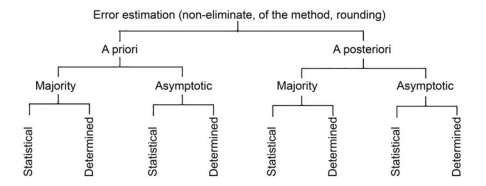
In constructing real computational processes of computations, $\varepsilon$-solution is often used by some estimates of global error, its component and process time. Herewith, they distinguish estimates in the following way: a priori and a posteriori, majorizing and asymptotic, and determinate and stochastic. The possibility and advisability of these estimates using and the methods of their construction depend on the type, structure, and accuracy of a priori data, the problem, and the CA from that why the estimate is computed, and it also depends on the computational resources [114,238].

Majorizing a priori estimate guarantees the upper bound of the estimated deriv atives, and they are performed through known derivatives. Their computation does not require some significant computational expenses, but the value of estimates are often overrated; therefore, the conclusions based on them as for the possibility of computing of the solution under the conditions $(2.1)$ and $(2.2)$ may be false.

Asymptotic estimates approximate the estimated derivative. The variability of the parameter can be achieved by the desirable estimate proximity to the estimated derivative, but the computation of such estimates is related to significant computational expenses, and these estimates are usually a posteriori.

In the algorithmic support of solving problems under the conditions (2.1) and (2.2), given the properties of the estimates, it must be expected the possibility of computing of the various types of estimates of characteristics $E\left(E_{\mathrm{u}}, E_{\mu}, E_{\tau}\right)$ [238]. By the relaxed constraints (2.1) and (2.2), less precise and less complex (computational) estimates may be sufficient. By the tighten constrains (2.1) and (2.2), asymptotic (a posteriori) estimates are used. For example, the condition (2.2) may apply strict requirements to the accuracy of estimates of computational process parameters that are computed on the basis of errors estimate of the solution.

数学代写|优化算法代写optimization algorithms代考|Classes of Computational Problems, Informational

In the given technology of constructing problems solution per time that does not exceed the given $T$, available information plays a great significance. The more a priori information of different principles is known on the problem and algorithm uses it, the more accuracy effective and time it can be solved.

Note that the effectiveness of the algorithms is determined by the estimate of their characteristics so that the estimates should be of high quality (constants that are included in majorizing estimates of errors, accurate, estimates, unimprovable, etc.). And yet even high-quality estimates are constructed on a class of problems. And the wider this class is, the less suitable this estimate may be for a particular problem. Therefore, it is important to have a classification of problems that considers the additional a priori information. This will make a possibility to “select” such a class for a solved problem that is most likely to be used to obtain the required solution of a certain quality.

Consequently, the improvement of the quality of solving problems depends on the “narrowing” of the class of problems to which the solved problem belongs and the building of algorithms of such solving problems and the most accurate estimates of their characteristics.

However, it is not always possible to obtain $\varepsilon$-solution of some problems (although the total input information may be enough for this) using the given technology, or it cannot be checked that the solution was achieved. In these cases, it is important to have algorithms that are accuracy optimal (all available information on the problem is used as much as possible to improve accuracy) and a posteriori error estimates (that are more accurate next to a priori ones).

On the back of the accuracy optimal algorithm of this solving problem and a posteriori estimate of the error, it is often possible to obtain a solution that satisfies the user or draw a conclusion that it was not possible to obtain such a solution. We consider key principles of the problems classification and algorithms through the examples of some specific classes of problems of computational and applied mathematics.

Computational Problem - an overview | ScienceDirect Topics
数学代写|优化算法代写optimization algorithms代考| Complexity of Real Computation Processes

优化算法代写

数学代写|优化算法代写optimization algorithms代考|On the Computer Constructing Technology

建设方案(选择)吨- 有效的计算算法取决于许多因素(类别问题、输入数据、问题的维度和特征、用户可用的计算资源、约束(2.1)、(2.2)和(2.3));因此,在类问题中F,建议在计算[14]的上下文中区分具有共同特征的众多(子类)问题:

  • 计算量小、处理时间适度限制的一次性问题
  • 需要实时解决的问题(或一系列问题)
  • 需要在实际合理的时间内解决的大量计算问题(传统计算机无法实现)

条件 (2.1)、(2.2) 和 (2.3) 的性能取决于问题的陈述,可以通过选择以下计算资源组合之一来实现:X,(X,一世n),(X,是),(X,是,一世n). 在前两种情况下,计算机的可能性是固定的。在第一种情况下,信息一世n也是固定的;算法及其参数的选择满足条件(2.1)、(2.2)和(2.3);在第二个中,仍然可以选择集合一世n对于这种类型的信息运营商。第三种情况,信息是固定的,除了算法,还可以选择计算机的参数。第四种情况,使用所有计算资源。

第一组问题可以通过选择来解决X或者(X,一世n)常规顺序计算机。因此,可以致力于计算模型的三个层次的细化。在第一层,有专注于类的算法F利用信息解决问题一世n. 因此,支持:近似、稳定性、近似解的收敛性、给定输入信息达到一定精度的可能性,以及作为问题大小(输入数据量)函数的计算量。在这个级别,有可能发现计算的不可能性e- 使用特定输入数据的解决方案,并且可能有可能澄清问题的类别和输入信息的要求,以提供一定精度的近似解决方案,并且可以(在这方面)选择新的算法.
第二个层次(detalization)是与使用众多元素有关是(机器字长,舍入规则)来计算舍入的误差估计。于此,众多一种(e)可以定义为在某些算法的可取性的情况下使用从众数中得出的结论一种(e)以节省处理时间。
在第三层,计算算法是用于计算e- 某台计算机上的解决方案,时间吨(e)和记忆米(e)[114]估计。
变种(X,是)和(X,是,一世n)特定于第二组问题,例如,使用专用计算机进行数字信号处理和数字图像处理。为了实现高速率,计算机架构与计算算法保持一致[131,277].

可以使用计算组织的第三或第四变体来解决第三组的问题。因此,可以使用单一用途的高端计算机 [220] 和所有用途的计算机 [199]。

数学代写|优化算法代写optimization algorithms代考|Specificity of Using Characteristic Estimates

在构建计算的真实计算过程时,e-solution 经常被一些全局误差、它的组成部分和处理时间的估计所使用。因此,他们以以下方式区分估计:先验和后验,主要和渐近,确定和随机。这些估计使用的可能性和可取性及其构建方法取决于先验数据的类型、结构和准确性、问题以及计算估计的 CA,还取决于计算资源[114,238]。

对先验估计进行大数化保证了估计导数的上限,并且它们是通过已知的导数来执行的。他们的计算不需要一些重大的计算费用,但估计的价值往往被高估了;因此,基于它们的结论关于在条件下计算解的可能性(2.1)和(2.2)可能是假的。

渐近估计近似估计导数。参数的可变性可以通过接近估计导数的理想估计来实现,但是这种估计的计算涉及大量的计算费用,并且这些估计通常是后验的。

在条件(2.1)和(2.2)下解决问题的算法支持中,给定估计的属性,必须预期计算各种类型的特征估计的可能性和(和在,和μ,和τ)[238]。通过放宽约束(2.1)和(2.2),不太精确和不太复杂(计算)的估计可能就足够了。通过紧约束(2.1)和(2.2),使用渐近(后验)估计。例如,条件 (2.2) 可以对计算过程参数的估计精度应用严格的要求,这些参数是根据解的误差估计计算的。

数学代写|优化算法代写optimization algorithms代考|Classes of Computational Problems, Informational

在给定的每次构造问题解决方案的技术中,不超过给定的吨, 可用信息具有重要意义。对问题和算法使用的不同原理的先验信息了解得越多,解决问题的准确性和效率就越高。

请注意,算法的有效性取决于对其特征的估计,因此估计应该是高质量的(包含在误差估计中的常量、准确、估计、不可改进等)。然而,即使是高质量的估计也是建立在一类问题上的。并且这个类越广泛,这个估计就越不适合特定问题。因此,重要的是对问题进行分类,考虑额外的先验信息。这将有可能为已解决的问题“选择”这样一个类,该类最有可能用于获得特定质量的所需解决方案。

因此,解决问题质量的提高取决于对所解决问题所属问题类别的“缩小”以及此类解决问题的算法的构建以及对其特征的最准确估计。

然而,并不总是能够获得e- 使用给定技术解决某些问题(尽管总的输入信息可能就足够了),或者无法检查解决方案是否已实现。在这些情况下,重要的是要有准确度最优的算法(尽可能使用有关问题的所有可用信息来提高准确度)和后验误差估计(比先验误差更准确)。

在这个求解问题的精度最优算法和误差的后验估计的背后,往往可以得到一个让用户满意的解,或者得出不可能得到这样一个解的结论。我们通过一些特定类别的计算和应用数学问题的例子来考虑问题分类和算法的关键原则。

数学代写|优化算法代写optimization algorithms代考 请认准statistics-lab™

统计代写请认准statistics-lab™. statistics-lab™为您的留学生涯保驾护航。

金融工程代写

金融工程是使用数学技术来解决金融问题。金融工程使用计算机科学、统计学、经济学和应用数学领域的工具和知识来解决当前的金融问题,以及设计新的和创新的金融产品。

非参数统计代写

非参数统计指的是一种统计方法,其中不假设数据来自于由少数参数决定的规定模型;这种模型的例子包括正态分布模型和线性回归模型。

广义线性模型代考

广义线性模型(GLM)归属统计学领域,是一种应用灵活的线性回归模型。该模型允许因变量的偏差分布有除了正态分布之外的其它分布。

术语 广义线性模型(GLM)通常是指给定连续和/或分类预测因素的连续响应变量的常规线性回归模型。它包括多元线性回归,以及方差分析和方差分析(仅含固定效应)。

有限元方法代写

有限元方法(FEM)是一种流行的方法,用于数值解决工程和数学建模中出现的微分方程。典型的问题领域包括结构分析、传热、流体流动、质量运输和电磁势等传统领域。

有限元是一种通用的数值方法,用于解决两个或三个空间变量的偏微分方程(即一些边界值问题)。为了解决一个问题,有限元将一个大系统细分为更小、更简单的部分,称为有限元。这是通过在空间维度上的特定空间离散化来实现的,它是通过构建对象的网格来实现的:用于求解的数值域,它有有限数量的点。边界值问题的有限元方法表述最终导致一个代数方程组。该方法在域上对未知函数进行逼近。[1] 然后将模拟这些有限元的简单方程组合成一个更大的方程系统,以模拟整个问题。然后,有限元通过变化微积分使相关的误差函数最小化来逼近一个解决方案。

tatistics-lab作为专业的留学生服务机构,多年来已为美国、英国、加拿大、澳洲等留学热门地的学生提供专业的学术服务,包括但不限于Essay代写,Assignment代写,Dissertation代写,Report代写,小组作业代写,Proposal代写,Paper代写,Presentation代写,计算机作业代写,论文修改和润色,网课代做,exam代考等等。写作范围涵盖高中,本科,研究生等海外留学全阶段,辐射金融,经济学,会计学,审计学,管理学等全球99%专业科目。写作团队既有专业英语母语作者,也有海外名校硕博留学生,每位写作老师都拥有过硬的语言能力,专业的学科背景和学术写作经验。我们承诺100%原创,100%专业,100%准时,100%满意。

随机分析代写


随机微积分是数学的一个分支,对随机过程进行操作。它允许为随机过程的积分定义一个关于随机过程的一致的积分理论。这个领域是由日本数学家伊藤清在第二次世界大战期间创建并开始的。

时间序列分析代写

随机过程,是依赖于参数的一组随机变量的全体,参数通常是时间。 随机变量是随机现象的数量表现,其时间序列是一组按照时间发生先后顺序进行排列的数据点序列。通常一组时间序列的时间间隔为一恒定值(如1秒,5分钟,12小时,7天,1年),因此时间序列可以作为离散时间数据进行分析处理。研究时间序列数据的意义在于现实中,往往需要研究某个事物其随时间发展变化的规律。这就需要通过研究该事物过去发展的历史记录,以得到其自身发展的规律。

回归分析代写

多元回归分析渐进(Multiple Regression Analysis Asymptotics)属于计量经济学领域,主要是一种数学上的统计分析方法,可以分析复杂情况下各影响因素的数学关系,在自然科学、社会和经济学等多个领域内应用广泛。

MATLAB代写

MATLAB 是一种用于技术计算的高性能语言。它将计算、可视化和编程集成在一个易于使用的环境中,其中问题和解决方案以熟悉的数学符号表示。典型用途包括:数学和计算算法开发建模、仿真和原型制作数据分析、探索和可视化科学和工程图形应用程序开发,包括图形用户界面构建MATLAB 是一个交互式系统,其基本数据元素是一个不需要维度的数组。这使您可以解决许多技术计算问题,尤其是那些具有矩阵和向量公式的问题,而只需用 C 或 Fortran 等标量非交互式语言编写程序所需的时间的一小部分。MATLAB 名称代表矩阵实验室。MATLAB 最初的编写目的是提供对由 LINPACK 和 EISPACK 项目开发的矩阵软件的轻松访问,这两个项目共同代表了矩阵计算软件的最新技术。MATLAB 经过多年的发展,得到了许多用户的投入。在大学环境中,它是数学、工程和科学入门和高级课程的标准教学工具。在工业领域,MATLAB 是高效研究、开发和分析的首选工具。MATLAB 具有一系列称为工具箱的特定于应用程序的解决方案。对于大多数 MATLAB 用户来说非常重要,工具箱允许您学习应用专业技术。工具箱是 MATLAB 函数(M 文件)的综合集合,可扩展 MATLAB 环境以解决特定类别的问题。可用工具箱的领域包括信号处理、控制系统、神经网络、模糊逻辑、小波、仿真等。

R语言代写问卷设计与分析代写
PYTHON代写回归分析与线性模型代写
MATLAB代写方差分析与试验设计代写
STATA代写机器学习/统计学习代写
SPSS代写计量经济学代写
EVIEWS代写时间序列分析代写
EXCEL代写深度学习代写
SQL代写各种数据建模与可视化代写

数学代写|优化算法代写optimization algorithms代考|Analytic Computational Complexity

如果你也在 怎样代写优化算法optimization algorithms这个学科遇到相关的难题,请随时右上角联系我们的24/7代写客服。

优化算法可分为使用导数的算法和不使用导数的算法。经典的算法使用目标函数的一阶导数,有时也使用二阶导数。

优化算法对深度学习很重要。一方面,训练一个复杂的深度学习模型可能需要数小时、数天甚至数周。优化算法的性能直接影响到模型的训练效率。另一方面,了解不同优化算法的原理及其超参数的作用,我们就能有针对性地调整超参数,提高深度学习模型的性能。

statistics-lab™ 为您的留学生涯保驾护航 在代写优化算法optimization algorithms方面已经树立了自己的口碑, 保证靠谱, 高质且原创的统计Statistics代写服务。我们的专家在代写优化算法optimization algorithms代写方面经验极为丰富,各种代写优化算法optimization algorithms相关的作业也就用不着说。

我们提供的优化算法optimization algorithms及其相关学科的代写,服务范围广, 其中包括但不限于:

  • Statistical Inference 统计推断
  • Statistical Computing 统计计算
  • Advanced Probability Theory 高等概率论
  • Advanced Mathematical Statistics 高等数理统计学
  • (Generalized) Linear Models 广义线性模型
  • Statistical Machine Learning 统计机器学习
  • Longitudinal Data Analysis 纵向数据分析
  • Foundations of Data Science 数据科学基础
A systematic literature review of Linked Data‐based recommender systems -  Figueroa - 2015 - Concurrency and Computation: Practice and Experience -  Wiley Online Library
数学代写|优化算法代写optimization algorithms代考|Analytic Computational Complexity

数学代写|优化算法代写optimization algorithms代考|Input Information, Algorithms, and Complexity

Consider the idealized computation model: Information $I_{n}(f)$ is given accurately, and the model $c$ is fixed. Here are some characteristics that are related to the lower and upper estimates of the error on the example of the passive pure minimax strategy $[102,253]$ (see Chap. 1 for more details):

  • $\rho_{\mu}(F, a)=\sup {f \in F} \rho\left(E{\mu}\left(I_{n}(f)\right), a\right)$ is an error of algorithm $a \in A$ on the class of the problems $F$ using information $I_{n}(f)$ (global error [270]).
  • $\rho_{\mu}(F, A)=\inf {a \in A} \rho{\mu}(F, a)$ is a lower boundary of error of algorithms of class $A$ in the class of problems $F$ using information $I_{n}(f)$ (radius of information [270])
    If there is an algorithm $a_{0} \in A$ for which $\rho_{\mu}\left(F, a_{0}\right)=\rho_{\mu}(F, A)$, then it is called accuracy optimal in class $F$ using information $I_{n}(f)$.

The narrowing of the $F$ class that is provided by the incompleteness of information (in relation to $f \in F) F_{n}(f)=\left{\varphi: I_{n}(\varphi)=I_{n}(f), \varphi, f \in F\right}$ allows to introduce the characteristics that are equivalent to the mentioned one above: $\rho_{\mu}\left(F_{n}(f), a\right)$ and $\rho_{\mu}\left(F_{n}(f), A\right)$, which are also called the local error and the local radius of information [270], respectively.

Let $U(f)$ be the multitude of solving problems from $F_{n}(f)$, and $\gamma(f)$ is the center of this multitude (the Chebyshev center). The algorithm $a^{\gamma} \in A$ is called a central one if $a^{y}\left(I_{n}(f)\right)=\gamma(f)$. These algorithms are accuracy optimal. Their important quality is that they minimize the local error of the algorithm:
$$
\inf {a \in A} \sup {\varphi \in F_{n}(f)} \rho_{\mu}\left(I_{n}(f), a\right)=\rho_{\mu}\left(I_{n}(f), a^{\gamma}\right)=\operatorname{rad} U(f) .
$$
Note that $A(\varepsilon) \neq \varnothing$ only when $\rho_{\mu}\left(F_{n}(f), A\right)<\varepsilon$.
Consider that class $A$ contains stable congruent algorithms and
$$
\rho_{\mu}\left(F_{n}(f), a\right) \rightarrow 0 \text { при } n \rightarrow \infty
$$
The algorithm $a$ is called asymptotically accuracy optimal (accuracy order optimal) if the condition is performed:
$$
\rho_{\mu}\left(F_{n}(f), A\right) / \rho_{\mu}\left(F_{n}(f), a\right) \rightarrow 1(\leq \text { const }), \quad n \rightarrow \infty
$$
Let $A(\varepsilon) \neq \varnothing$. The value $T(F, a, \varepsilon)=\sup {f \in F} T\left(I{n}(f), a, \varepsilon\right)$ is called $\varepsilon$-complexity of the algorithm $a \in A(\varepsilon)$ on the class of problems $F$ using information $I_{n}(f)$; $T(F, A, \varepsilon)=\inf {a \in A(\varepsilon)} T(F, a, \varepsilon)$ is $\varepsilon$-complexity of class $F$ problems using algorithms $A(\varepsilon)$ and information $I{n}(f)$. If there is an algorithm $a^{0} \in A(\varepsilon)$ for which

$T\left(F, a^{0}, \varepsilon\right)=T(F, A, \varepsilon)$, then it is called complexity optimal algorithm in this computational model. As in the case of error, it is possible to enter characteristics $T\left(F_{n}(f), a, \varepsilon\right)$ and $T\left(F_{n}(f), A, \varepsilon\right)$ on the class $F_{n}(f)$ and definitions of the optimal, asymptotically optimal, and complexity order optimal of the algorithm.

The mentioned characteristics are about the so-called “worst”-case model. The estimates are focused on the “worst” (the most complex) problem of the class. Of course, these estimates are guaranteed, and they are achieved on any problem of class $\Pi$, but this problem can be atypical for a given class. Therefore, there are some possible situations where the $\varepsilon$-solution can be obtained at lower expenses $(T)$. Consequently, in order to minimize the computational complexity of the $\varepsilon$-solution construction, the current question of the problems of classes narrowing, the ways where input data is presented, and the use of a priori information on a problem is relevant.

数学代写|优化算法代写optimization algorithms代考|Computer Architecture and the Complexity

There is an opinion (see, for example, [218]) that the optimization of the mathematical support of applied problems and the progress of computing techniques make equal contributions to the increasing possibilities of complex solving problems, in a point of fact in decreasing the computational complexity.

Consider the effect of rounding of the numbers on the computational complexity. Hypothesis [22] on that it is enough to compute the estimate of function $f$ for obtaining the solution with accuracy $O(\varepsilon)$ and perform intermediate computations in implemented CA with $O\left(\ln \varepsilon^{-1}\right)$ binary digit bits found confirmation in solving many problems $[42,106,114]$.

Thus, in the building of the $\varepsilon$-solution, the program uses numeric arrays with a total volume of $N$ numbers, and then memory $O\left(N \ln \varepsilon^{-1}\right)$ is required to store them.
Next, there is a possibility to consider the example of separate classes of problems and how the rounding error affects the possibility of $\varepsilon$-solution computation and the complexity of CP.
Let
$$
\begin{gathered}
\rho\left(E_{\mathrm{H}}\left(I_{n}(f), a, c\right) \leq \varepsilon_{1}<\varepsilon\right. \ \rho\left(E_{\mu \tau}\left(I_{n}(f), a, c\right)>\varepsilon_{2}, \quad \varepsilon_{2}=\varepsilon-\varepsilon_{1}\right.
\end{gathered}
$$
where $E_{\mu \tau}=E_{\mu}+E_{\tau}, a \in A$, and the relations are performed (in a point of fact in the numerical integration of $\mathrm{ODE}$, the computation of integrals and other classes of problems) $[106,114]$;

$$
E_{\mu}=O\left(n^{-p}\right), \quad E_{\tau}=O\left(n 2^{-\tau}\right),
$$
where $p$ is the order of the numerical method accuracy, and $\tau$ is the length of the mantissa in binary number notation in the floating-point mode. Herewith,
$$
\varepsilon_{\mu \tau}^{0}(\tau)=\min {n} \rho\left(E{\mu z}\left(I_{n}(f), a, c\right)=O\left(n_{0}^{-p}(\tau)\right),\right.
$$
where $n_{0}(\tau)=O\left(2^{\tau /(p+1)}\right)$, and $E_{\mu}\left(n_{0}(\tau)\right)=O\left(n_{0}^{-p}(\tau)\right), E_{\tau}\left(n_{0}(\tau)\right)=O\left(n_{0}^{-p}(\tau)\right)$.
Method error predominates when $n \ll n_{0}$. It can be decreased using optimal sets $I_{n}$, increasing $n$ (considering (2.10)), using accuracy optimal and close to them CA, moving to another class of input data $I_{n}$ (to increase the order of accuracy) and relevant CA.

The rounding error predominates when $n \gg n_{0}$. The decreasing $\rho\left(E_{\mu \mathrm{r}}\right)$ can be achieved by immediate increasing $n$ (considering $(2.10)$ ) or using the same capabilities as when $n \gg n_{0}$ (except increasing), as well as by increasing of $\tau$. From the relations (2.9) and (2.10), it follows that the performance of the constrain $\varepsilon_{\mu \tau}^{0} \leq \varepsilon_{2}$ is related to the conditions:
$$
n=O\left(\varepsilon_{2}^{-1 / p}\right), \quad \tau=O\left(\log \varepsilon_{2}^{-1}\right), \quad \varepsilon_{2} \rightarrow 0
$$
Consider the case (2.6). Let $\varepsilon$-solution be computed on the one processor using a linear computational algorithm per hour:
$$
T(\varepsilon)=T_{l}(\varepsilon)+T_{a}(\varepsilon),
$$
where $T_{I}(\varepsilon)$ is the process time of computation of the set of functionals $I_{n}(f)$ (information complexity), and $T_{a}(\varepsilon)$ is the process time of CA implementation for given information $I_{n}(f)$ (combinatorial complexity). Thus,
$$
\begin{gathered}
T_{l}(\varepsilon)=n(\varepsilon) \beta_{f}(\varepsilon) \alpha(\varepsilon), \
T_{a}(\varepsilon)=n(\varepsilon) \beta_{a} \alpha(\varepsilon),
\end{gathered}
$$
where $\alpha(\varepsilon)$ is the time performance of the “mean” operation in the computation of $\varepsilon$ solution; $\beta_{f}(\varepsilon)$ is an average number of computation operations of the functional $i_{j}$; and $\beta_{a}$ is an average number of operations that are related to the use of one function in implementation of CA.

Note that $\beta_{f}(\varepsilon)$ does not depend on $\varepsilon$ if the functionals in $I_{n}(f)$ can be computed closely to the accurate arithmetical operations. Then,
$$
T(\varepsilon)=n(\varepsilon) \beta \alpha(\varepsilon), \quad \beta=\beta_{f}+\beta_{a} .
$$

数学代写|优化算法代写optimization algorithms代考|Optical Models of Computations

Optical Models of Computations Dynamic holography [102] is a promising way of implementing a variety of optical converters. For instance, the effect of the energy transfer of a beam of light into another coherent light of beam that goes in the other direction (courtesy of their transverse in a dynamic environment) is an optical analogue of the transistor. It is possible to control the temporal variations in its intensity by changing the intensity of the amplifying beam. In another variant of the optical analogue of the electronic transistor, such control is achieved by changing not the intensity but the phase of the intensity beam.

Another example can be an optical switching device that is similar to a high-speed electronic commutator that is an inherent part of the most important devices of the computing techniques.

The advantage of holography is the possibility of a single transformation of the most complex images and not just the primary plane or spherical waves.

For today, the experiments have been performed on the creation of optical of bistable devices that switch $10^{-12}$ with elements of optical fiber communication lines, the information of which is moved with the help of optical solutions with the duration of reaching $10^{-13}$. With such a switching time, the productivity of a digital optical processor $10^{5}-10^{6}$ has simultaneous channels that would be equal to $10^{18}$ operations per second; in other words, it is on six order higher than the productive potential of electronic schemes. Examples of primitive actions for an optical computer include addition and subtraction of mappings, computation of Fourier transform, mapping identification, and so on.

Development of Multimodal Machine Learning Potentials: Toward a  Physics-Aware Artificial Intelligence | Accounts of Chemical Research
数学代写|优化算法代写optimization algorithms代考|Analytic Computational Complexity

优化算法代写

数学代写|优化算法代写optimization algorithms代考|Input Information, Algorithms, and Complexity

考虑理想化的计算模型:信息一世n(F)准确给出,模型C是固定的。以下是与被动纯极小极大策略示例中误差的上下估计相关的一些特征[102,253](有关详细信息,请参阅第 1 章):

  • ρμ(F,一种)=支持F∈Fρ(和μ(一世n(F)),一种)是算法错误一种∈一种关于问题的类别F使用信息一世n(F)(全局错误 [270])。
  • ρμ(F,一种)=信息一种∈一种ρμ(F,一种)是类算法的误差下界一种在问题类别中F使用信息一世n(F)(信息半径[270])
    如果有算法一种0∈一种为此ρμ(F,一种0)=ρμ(F,一种),则称其为类中精度最优F使用信息一世n(F).

收窄的F由信息的不完整性提供的类别(关于f \in F) F_{n}(f)=\left{\varphi: I_{n}(\varphi)=I_{n}(f), \varphi, f \in F\right}f \in F) F_{n}(f)=\left{\varphi: I_{n}(\varphi)=I_{n}(f), \varphi, f \in F\right}允许引入与上述特征等效的特征:ρμ(Fn(F),一种)和ρμ(Fn(F),一种),也分别称为局部误差和局部信息半径[270]。

让在(F)成为众多解决问题的人Fn(F), 和C(F)是这群人的中心(切比雪夫中心)。算法一种C∈一种被称为中心的,如果一种是(一世n(F))=C(F). 这些算法是精度最优的。它们的重要品质是它们使算法的局部误差最小化:
信息一种∈一种支持披∈Fn(F)ρμ(一世n(F),一种)=ρμ(一世n(F),一种C)=拉德⁡在(F).
注意一种(e)≠∅只有当ρμ(Fn(F),一种)<e.
考虑那个类一种包含稳定的全等算法和
приρμ(Fn(F),一种)→0 在 n→∞
算法一种如果执行以下条件,则称为渐近精度最优(精度阶最优):
ρμ(Fn(F),一种)/ρμ(Fn(F),一种)→1(≤ 常量 ),n→∞
让一种(e)≠∅. 价值吨(F,一种,e)=支持F∈F吨(一世n(F),一种,e)叫做e- 算法的复杂性一种∈一种(e)关于问题的类别F使用信息一世n(F); 吨(F,一种,e)=信息一种∈一种(e)吨(F,一种,e)是e- 类的复杂性F使用算法的问题一种(e)和信息一世n(F). 如果有算法一种0∈一种(e)为此

吨(F,一种0,e)=吨(F,一种,e),则在该计算模型中称为复杂度最优算法。在出错的情况下,可以输入特征吨(Fn(F),一种,e)和吨(Fn(F),一种,e)在课堂上Fn(F)以及算法的最优、渐近最优和复杂度最优的定义。

提到的特征是关于所谓的“最坏”情况模型。估计集中在班级中“最糟糕”(最复杂)的问题上。当然,这些估计是有保证的,并且在任何类问题上都可以实现圆周率,但是对于给定的类,这个问题可能是非典型的。因此,有一些可能的情况e- 可以以较低的费用获得解决方案(吨). 因此,为了最小化计算复杂度e-解决方案的构建,当前的类别缩小问题,输入数据的呈现方式以及对问题的先验信息的使用是相关的。

数学代写|优化算法代写optimization algorithms代考|Computer Architecture and the Complexity

有一种观点(例如,参见 [218])认为,应用问题的数学支持的优化和计算技术的进步对增加复杂解决问题的可能性做出了同等贡献,事实上在减少计算复杂度。

考虑数字舍入对计算复杂度的影响。假设 [22] 计算函数的估计就足够了F准确地获得解决方案这(e)并在已实现的 CA 中执行中间计算这(ln⁡e−1)二进制数字位在解决许多问题中得到确认[42,106,114].

因此,在建设e-解决方案,该程序使用总体积为的数字数组ñ数字,然后记忆这(ñln⁡e−1)需要存储它们。
接下来,有可能考虑不同类别问题的示例以及舍入误差如何影响e- 解计算和 CP 的复杂性。

ρ(和H(一世n(F),一种,C)≤e1<e ρ(和μτ(一世n(F),一种,C)>e2,e2=e−e1
在哪里和μτ=和μ+和τ,一种∈一种, 并执行关系(实际上在数值积分中这D和, 积分计算和其他类型的问题)[106,114];和μ=这(n−p),和τ=这(n2−τ),
在哪里p是数值方法精度的阶数,并且τ是浮点模式下二进制数表示法的尾数长度。特此,
eμτ0(τ)=分钟nρ(和μ和(一世n(F),一种,C)=这(n0−p(τ)),
在哪里n0(τ)=这(2τ/(p+1)), 和和μ(n0(τ))=这(n0−p(τ)),和τ(n0(τ))=这(n0−p(τ)).
方法错误占主导地位时n≪n0. 可以使用最优集来减少它一世n, 增加n(考虑(2.10)),使用最佳精度并接近它们 CA,移动到另一类输入数据一世n(以提高准确性的顺序)和相关的 CA。

舍入误差占主导地位时n≫n0. 递减ρ(和μr)可以通过立即增加来实现n(考虑到(2.10)) 或使用与时相同的功能n≫n0(除了增加),以及通过增加τ. 从关系式 (2.9) 和 (2.10) 可以看出,约束的性能eμτ0≤e2与条件有关:
n=这(e2−1/p),τ=这(日志⁡e2−1),e2→0
考虑情况(2.6)。让e- 每小时使用线性计算算法在一个处理器上计算解决方案:
吨(e)=吨l(e)+吨一种(e),
在哪里吨一世(e)是函数集计算的处理时间一世n(F)(信息复杂性),以及吨一种(e)是给定信息的 CA 实施的过程时间一世n(F)(组合复杂性)。因此,
吨l(e)=n(e)bF(e)一种(e), 吨一种(e)=n(e)b一种一种(e),
在哪里一种(e)是计算中“均值”操作的时间性能e解决方案;bF(e)是函数的平均计算操作数一世j; 和b一种是与在 CA 实现中使用一个功能相关的平均操作数。

注意bF(e)不依赖于e如果函数在一世n(F)可以接近精确的算术运算来计算。然后,
吨(e)=n(e)b一种(e),b=bF+b一种.

数学代写|优化算法代写optimization algorithms代考|Optical Models of Computations

计算的光学模型 动态全息术 [102] 是一种实现各种光学转换器的有前途的方法。例如,一束光束的能量转移到另一个相干光束的另一个方向上的效果(由它们在动态环境中的横向提供)是晶体管的光学模拟。可以通过改变放大光束的强度来控制其强度的时间变化。在电子晶体管的光学模拟的另一个变体中,这种控制是通过不改变强度而是改变强度光束的相位来实现的。

另一个示例可以是类似于高速电子换向器的光开关设备,它是计算技术中最重要设备的固有部分。

全息术的优点是可以对最复杂的图像进行一次变换,而不仅仅是初级平面波或球面波。

今天,已经进行了关于创建可切换的双稳态设备的光学实验10−12带有光纤通信线路的元件,其信息在光学解决方案的帮助下移动,持续时间达到10−13. 有了这样的切换时间,数字光学处理器的生产力105−106具有等于​​的同时通道1018每秒操作数;换句话说,它比电子方案的生产潜力高出六个数量级。光学计算机的原始动作示例包括映射的加法和减法、傅里叶变换的计算、映射识别等。

数学代写|优化算法代写optimization algorithms代考 请认准statistics-lab™

统计代写请认准statistics-lab™. statistics-lab™为您的留学生涯保驾护航。

金融工程代写

金融工程是使用数学技术来解决金融问题。金融工程使用计算机科学、统计学、经济学和应用数学领域的工具和知识来解决当前的金融问题,以及设计新的和创新的金融产品。

非参数统计代写

非参数统计指的是一种统计方法,其中不假设数据来自于由少数参数决定的规定模型;这种模型的例子包括正态分布模型和线性回归模型。

广义线性模型代考

广义线性模型(GLM)归属统计学领域,是一种应用灵活的线性回归模型。该模型允许因变量的偏差分布有除了正态分布之外的其它分布。

术语 广义线性模型(GLM)通常是指给定连续和/或分类预测因素的连续响应变量的常规线性回归模型。它包括多元线性回归,以及方差分析和方差分析(仅含固定效应)。

有限元方法代写

有限元方法(FEM)是一种流行的方法,用于数值解决工程和数学建模中出现的微分方程。典型的问题领域包括结构分析、传热、流体流动、质量运输和电磁势等传统领域。

有限元是一种通用的数值方法,用于解决两个或三个空间变量的偏微分方程(即一些边界值问题)。为了解决一个问题,有限元将一个大系统细分为更小、更简单的部分,称为有限元。这是通过在空间维度上的特定空间离散化来实现的,它是通过构建对象的网格来实现的:用于求解的数值域,它有有限数量的点。边界值问题的有限元方法表述最终导致一个代数方程组。该方法在域上对未知函数进行逼近。[1] 然后将模拟这些有限元的简单方程组合成一个更大的方程系统,以模拟整个问题。然后,有限元通过变化微积分使相关的误差函数最小化来逼近一个解决方案。

tatistics-lab作为专业的留学生服务机构,多年来已为美国、英国、加拿大、澳洲等留学热门地的学生提供专业的学术服务,包括但不限于Essay代写,Assignment代写,Dissertation代写,Report代写,小组作业代写,Proposal代写,Paper代写,Presentation代写,计算机作业代写,论文修改和润色,网课代做,exam代考等等。写作范围涵盖高中,本科,研究生等海外留学全阶段,辐射金融,经济学,会计学,审计学,管理学等全球99%专业科目。写作团队既有专业英语母语作者,也有海外名校硕博留学生,每位写作老师都拥有过硬的语言能力,专业的学科背景和学术写作经验。我们承诺100%原创,100%专业,100%准时,100%满意。

随机分析代写


随机微积分是数学的一个分支,对随机过程进行操作。它允许为随机过程的积分定义一个关于随机过程的一致的积分理论。这个领域是由日本数学家伊藤清在第二次世界大战期间创建并开始的。

时间序列分析代写

随机过程,是依赖于参数的一组随机变量的全体,参数通常是时间。 随机变量是随机现象的数量表现,其时间序列是一组按照时间发生先后顺序进行排列的数据点序列。通常一组时间序列的时间间隔为一恒定值(如1秒,5分钟,12小时,7天,1年),因此时间序列可以作为离散时间数据进行分析处理。研究时间序列数据的意义在于现实中,往往需要研究某个事物其随时间发展变化的规律。这就需要通过研究该事物过去发展的历史记录,以得到其自身发展的规律。

回归分析代写

多元回归分析渐进(Multiple Regression Analysis Asymptotics)属于计量经济学领域,主要是一种数学上的统计分析方法,可以分析复杂情况下各影响因素的数学关系,在自然科学、社会和经济学等多个领域内应用广泛。

MATLAB代写

MATLAB 是一种用于技术计算的高性能语言。它将计算、可视化和编程集成在一个易于使用的环境中,其中问题和解决方案以熟悉的数学符号表示。典型用途包括:数学和计算算法开发建模、仿真和原型制作数据分析、探索和可视化科学和工程图形应用程序开发,包括图形用户界面构建MATLAB 是一个交互式系统,其基本数据元素是一个不需要维度的数组。这使您可以解决许多技术计算问题,尤其是那些具有矩阵和向量公式的问题,而只需用 C 或 Fortran 等标量非交互式语言编写程序所需的时间的一小部分。MATLAB 名称代表矩阵实验室。MATLAB 最初的编写目的是提供对由 LINPACK 和 EISPACK 项目开发的矩阵软件的轻松访问,这两个项目共同代表了矩阵计算软件的最新技术。MATLAB 经过多年的发展,得到了许多用户的投入。在大学环境中,它是数学、工程和科学入门和高级课程的标准教学工具。在工业领域,MATLAB 是高效研究、开发和分析的首选工具。MATLAB 具有一系列称为工具箱的特定于应用程序的解决方案。对于大多数 MATLAB 用户来说非常重要,工具箱允许您学习应用专业技术。工具箱是 MATLAB 函数(M 文件)的综合集合,可扩展 MATLAB 环境以解决特定类别的问题。可用工具箱的领域包括信号处理、控制系统、神经网络、模糊逻辑、小波、仿真等。

R语言代写问卷设计与分析代写
PYTHON代写回归分析与线性模型代写
MATLAB代写方差分析与试验设计代写
STATA代写机器学习/统计学习代写
SPSS代写计量经济学代写
EVIEWS代写时间序列分析代写
EXCEL代写深度学习代写
SQL代写各种数据建模与可视化代写

数学代写|优化算法代写optimization algorithms代考| Algebraic Computing Complexity

如果你也在 怎样代写优化算法optimization algorithms这个学科遇到相关的难题,请随时右上角联系我们的24/7代写客服。

优化算法可分为使用导数的算法和不使用导数的算法。经典的算法使用目标函数的一阶导数,有时也使用二阶导数。

优化算法对深度学习很重要。一方面,训练一个复杂的深度学习模型可能需要数小时、数天甚至数周。优化算法的性能直接影响到模型的训练效率。另一方面,了解不同优化算法的原理及其超参数的作用,我们就能有针对性地调整超参数,提高深度学习模型的性能。

statistics-lab™ 为您的留学生涯保驾护航 在代写优化算法optimization algorithms方面已经树立了自己的口碑, 保证靠谱, 高质且原创的统计Statistics代写服务。我们的专家在代写优化算法optimization algorithms代写方面经验极为丰富,各种代写优化算法optimization algorithms相关的作业也就用不着说。

我们提供的优化算法optimization algorithms及其相关学科的代写,服务范围广, 其中包括但不限于:

  • Statistical Inference 统计推断
  • Statistical Computing 统计计算
  • Advanced Probability Theory 高等概率论
  • Advanced Mathematical Statistics 高等数理统计学
  • (Generalized) Linear Models 广义线性模型
  • Statistical Machine Learning 统计机器学习
  • Longitudinal Data Analysis 纵向数据分析
  • Foundations of Data Science 数据科学基础
Conceptual Framework Computational cost, Complexity, Accuracy are... |  Download Scientific Diagram
数学代写|优化算法代写optimization algorithms代考| Algebraic Computing Complexity

数学代写|优化算法代写optimization algorithms代考|Formal Computational Models

Turing machines (TM) [3] is a class of the most well-known formal models for the analysis of the problem of limited complexity. The problem is considered to be algorithmically solved if its solution can be built using the corresponding TM. It

should be noted that the class of problems that can be solved with TM is left to be solved moving from TM to another formal model [3,241, 271]. All problems of algebraic complexity are divided into two classes (the class $\mathrm{P}$ is a problem that can be solved with polynomial complexity on deterministic Turing machines (DTM), and the NP class is the class where the problems can be solved with polynomial complexity on nondeterministic Turing machines (NTM) [3]). As the characteristics of the computational complexity, computing time (number of steps that are necessary to use the solving problem of the algorithm) and memory (the amount of operating domain that is used by the algorithm) are used.

Here are some known relations between the time complexity $(T(n), n$ is the amount of input data) and by the amount of memory $(S(n))$ [249] that are obtained for TM.

Let DTIME $(T(n))$ (DSPACE $(S(n)))$ be a class of problem that suppose DTM per hour $T(n)$ (with a memory $(S(n)$ ). The classes of problems are determined likewise NTIME $(\cdot)$, NSPACE $(\cdot)$ for HTM. Then
$$
\begin{gathered}
\operatorname{DTIME}(T(n)) \subseteq \operatorname{NTIME}(T(n)) \
\operatorname{NTIME}(T(n)) \subseteq \operatorname{DTIME}\left(2^{O(T(n))}\right) \
\operatorname{DSPACE}(S(n)) \subseteq \operatorname{NSPACE}(S(n)) \
\operatorname{NSPACE}(S(n)) \subseteq \operatorname{DSPACE}\left(S^{2}(n)\right) \
\operatorname{NTIME}(T(n)) \subseteq \operatorname{DSPACE}(T(n)) \
\operatorname{DTIME}(T(n)) \subseteq \operatorname{DSPACE}\left(T(n) / \log _{2}(T(n))\right) \
\operatorname{NSPACE}(T(n)) \subseteq \operatorname{DTIME}\left(2^{O(S(n))}\right)
\end{gathered}
$$
An important example of complex problems is NP-complete problems. The problem $f$ is considered to be NP-completed if it belongs to the NP class and each NP problem can be polynomial complexity that is reduced to $f$. The central point in the theory of NP-completeness is whether or not the classes $\mathrm{P}$ and NP are congruent, in other words if the problem (from the class NP) is provided by practice that is related to problems (of class P) that can be solved. There are reasons to assume that the solution of the most complex problems of the NP class (NP-complete problems) requires (as it can be seen from the estimates) the deterministic exponential time; in other words, the classes P and NP are different. The NP-completeness of many problems is proved $[3,48]$. The difficulty is to prove that each NP problem can be polynomially transformed to this problem.

It should be noted that the definition of the NP class and the proof of the polynomial complexity of many “reset” problems had great practical importance. Together with practical valuation, it destroyed some illusions regarding the practical constructing of solving a problem that has a solution; it has been found that the existence of only one algorithm for solving a certain mass issue is not enough for

practice. On the other hand, the algorithms for which acceptable polynomial upper estimated were proved and found some practical use.

The basic possibility of classification by complexity is provided by the so-called theorems on the hierarchy. The hierarchy theorem for a given complexity (by time or memory) determines which decrease in the upper complexity estimate leads to the narrowing of the class of functions that can be computed with this complexity.

数学代写|优化算法代写optimization algorithms代考|Asymptotic Qualities of “Fast” Algorithms

The purpose of a lower complexity estimate construction is to prove that none of the algorithms in this computational model has less complexity of computation than the given function $\varphi(t)$. Unfortunately, the well-known “high” (nontrivial) lower estimates are perhaps the exception, not the rule.

The scheme of upper estimates of complexity constructing is as following. Based on some methods of solving problem, CA is built in a particular computational model, and it is proved that the computational complexity does not exceed some function from input data in the class. This function is called the upper estimate of the computational complexity of solving problem constructing.

There are several types of CA (which these estimates are implemented on). They are optimal, order optimal, and asymptotically optimal. Optimal CA corresponds to the case when the upper and lower boundaries are congruent. Two other types of CA concem, respectively, the estimates with the “accuracy to the multiplicative constant” and “accuracy to additive constants.” The practical use of algorithms is based on estimates that have an explicit specificity.

Consider these questions briefly. Let $A(0, X) \neq \varnothing A$ consider the computer model of sequential computations. Then
$$
T\left(I_{n}(f), X, Y\right)=T_{I}\left(I_{n}(f), Y\right)+T_{a}(X, Y),
$$
where $T_{I}(\cdot)=\sum_{1}^{r} \alpha_{i} n_{i}(n), T_{a}(\cdot)=\sum_{1}^{r} \alpha_{i} m_{i}(n, a), \alpha_{i}$ is a price of the $i$-operation from the model $c ; n_{i}(n), m_{i}(n, a)$ is the number of operations of the $i$-type that are necessary for the computation of the set of functionals $I_{n}(f)$ and the solution of the problem $f$ by the algorithm $a \in A$, provided that the set $I_{n}(f)$ is known; and $n$ is a number of functionals in the set. The values $T_{l}, T_{a}$ are called, respectively, informational and combinatorial (computational) complexities (solving computation) [270].

Note that the value $T$ depends essentially on $n$ and the character of the dependence $\left{n_{i}, m_{i}\right}$ from $n$. For example, by solving a system of $n$ linear equations, $A x=b$ by Gaussian elimination (for given $A, b) n_{i}=0, m_{i}=O\left(n^{3}\right), i=1,2$ (there is about the operations of addition and multiplication of two numbers).

In the general case, there is a possibility to assume that $n_{i}=O(n)$ (the functional $I_{n}(f)$ has a limited complexity) and $m_{i}(n)$ can be functions of $n$, for example, polynomial or exponential (or higher) complexity. Then the question arises on the

possibility of a solution computation with less computational complexity (see, for example, the class of NP-complete problems).

Of course, the character of dependence $m_{i}$ from $n$ is not determinative in the practical acceptability of the algorithm for solving a specific problem. It must be also considered that the constants in the functional dependences $m_{i}(n)$ can be that sort of algorithms with a lower order of complexity increasing, and advantage will be only for infinite values $n$. For example, offered algorithms of solving systems of linear algebraic equations for which $m_{i}=O\left(n^{\beta}\right), \beta<3$, have advantages over the complexity of Gaussian elimination for infinite values $n$. In addition, it is needed to pay attention to the possible loss of numerical stability of the algorithm. The fast Fourier transform (FFT) algorithm is used to multiply two numbers, and it has the complexity $O(n \log n)$ where $n$ is the number of binary digit bits for the number notation. The practical advantage of a high speed next to the traditional way of multiplication $\left(O\left(n^{2}\right)\right)$ is achieved for $n>100$.

数学代写|优化算法代写optimization algorithms代考|Accuracy and Complexity of Computations

The theory of analytic complexity is closely related to the theory of errors in the approximate solving problem. The value of the processing time is often determined by the requirements to the accuracy of the approximate solution; the relation of the components of the global error; the dependence of the error on the type, structure, volume of input data and their accuracy, bit grid of computer, and rounding rules; the type of error estimates; and the method of estimates constructing from below and from above. Therefore, there is a good reason to consider advisably these two characteristics: the error of the approximate solution and the process time [297, 301$]$.
Considering that it is difficult to build high lower and lower upper estimates in the given model of computation (when $E$ is a global error), some idealized models are considered that to consider only individual components of the global error (more often the errors of the method) and the influence of the individual components of computational models on error and complexity. For such incomplete models, it is possible to conclude the impossibility of constructing $\varepsilon$-solution based on this information.

The dependence of the approximate solution accuracy and the complexity of the $\varepsilon$-solution computation from the various components of the computational model will be considered next.

Solving quasiparticle band spectra of real solids using neural-network  quantum states | Communications Physics
数学代写|优化算法代写optimization algorithms代考| Algebraic Computing Complexity

优化算法代写

数学代写|优化算法代写optimization algorithms代考|Formal Computational Models

图灵机 (TM) [3] 是一类最著名的形式模型,用于分析有限复杂性问题。如果可以使用相应的 TM 构建解决方案,则认为该问题已通过算法解决。它

应该注意的是,可以用 TM 解决的问题类别有待从 TM 转移到另一个正式模型 [3,241, 271] 来解决。代数复杂度的所有问题都分为两类(类磷是可以在确定性图灵机 (DTM) 上用多项式复杂度解决的问题,而 NP 类是可以在非确定性图灵机 (NTM) 上用多项式复杂度解决问题的类 [3])。作为计算复杂度的特征,使用计算时间(使用算法解决问题所需的步骤数)和内存(算法使用的操作域的数量)。

以下是时间复杂度之间的一些已知关系(吨(n),n是输入数据量)和内存量(小号(n))[249] 是为 TM 获得的。

让 DTIME(吨(n))(空间(小号(n)))是假设每小时 DTM 的一类问题吨(n)(有记忆(小号(n))。问题的类别同样由 NTIME 确定(⋅), 空间(⋅)对于 HTM。然后
时间⁡(吨(n))⊆新时代⁡(吨(n)) 新时代⁡(吨(n))⊆时间⁡(2这(吨(n))) 空间⁡(小号(n))⊆空间⁡(小号(n)) 空间⁡(小号(n))⊆空间⁡(小号2(n)) 新时代⁡(吨(n))⊆空间⁡(吨(n)) 时间⁡(吨(n))⊆空间⁡(吨(n)/日志2⁡(吨(n))) 空间⁡(吨(n))⊆时间⁡(2这(小号(n)))
复杂问题的一个重要例子是 NP 完全问题。问题F如果它属于 NP 类,则认为它是 NP 完全的,并且每个 NP 问题都可以是多项式复杂度,可以简化为F. NP 完全性理论的中心点是类是否磷和 NP 是一致的,换句话说,如果问题(来自 NP 类)是由与可以解决的(P 类)问题相关的实践提供的。有理由假设解决最复杂的 NP 类问题(NP 完全问题)需要(从估计中可以看出)确定性指数时间;换句话说,类 P 和 NP 是不同的。证明了许多问题的NP完全性[3,48]. 难点在于证明每个 NP 问题都可以多项式转化为这个问题。

需要注意的是,NP 类的定义和许多“重置”问题的多项式复杂性的证明具有重要的实际意义。与实际评估一起,它打破了一些关于解决有解决方案的问题的实际构建的幻想;已经发现,仅存在一种算法来解决某个质量问题是不够的

实践。另一方面,证明了可接受多项式上估计的算法并发现了一些实际用途。

所谓的层次定理提供了按复杂性分类的基本可能性。给定复杂度(按时间或内存)的层次定理决定了上层复杂度估计中的哪个降低导致可以用这种复杂度计算的函数类别的缩小。

数学代写|优化算法代写optimization algorithms代考|Asymptotic Qualities of “Fast” Algorithms

较低复杂度估计构造的目的是证明该计算模型中没有一个算法的计算复杂度低于给定函数披(吨). 不幸的是,众所周知的“高”(非平凡)较低估计可能是例外,而不是规则。

构造复杂度的上估计方案如下。基于一些求解问题的方法,CA建立在特定的计算模型中,从类中的输入数据证明计算复杂度不超过某个函数。该函数称为求解问题构造的计算复杂度的上估计。

有几种类型的 CA(这些估计是在其上实现的)。它们是最优的、阶最优的和渐近最优的。最佳 CA 对应于上下边界一致的情况。其他两种类型的 CA 分别涉及“乘法常数的准确性”和“加法常数的准确性”的估计。算法的实际使用基于具有明确特异性的估计。

简要考虑这些问题。让一种(0,X)≠∅一种考虑顺序计算的计算机模型。然后
吨(一世n(F),X,是)=吨一世(一世n(F),是)+吨一种(X,是),
在哪里吨一世(⋅)=∑1r一种一世n一世(n),吨一种(⋅)=∑1r一种一世米一世(n,一种),一种一世是价格一世- 从模型操作C;n一世(n),米一世(n,一种)是操作的次数一世- 计算泛函集所必需的类型一世n(F)以及问题的解决方案F通过算法一种∈一种, 假设集合一世n(F)已知;和n是集合中的许多泛函。价值吨l,吨一种分别称为信息和组合(计算)复杂性(求解计算)[270]。

请注意,该值吨本质上取决于n和依赖的性质\left{n_{i}, m_{i}\right}\left{n_{i}, m_{i}\right}从n. 例如,通过求解一个系统n线性方程组,一种X=b通过高斯消去(对于给定的一种,b)n一世=0,米一世=这(n3),一世=1,2(关于两个数字的加法和乘法运算)。

在一般情况下,有可能假设n一世=这(n)(功能性一世n(F)具有有限的复杂性)和米一世(n)可以是n,例如,多项式或指数(或更高)复杂度。那么问题就出现在

计算复杂度较低的解计算的可能性(例如,参见 NP 完全问题的类别)。

当然,依赖的性格米一世从n在解决特定问题的算法的实际可接受性方面不是决定性的。还必须考虑函数依赖中的常数米一世(n)可以是具有较低复杂度增加的那种算法,并且优势将仅适用于无限值n. 例如,提供求解线性代数方程组的算法米一世=这(nb),b<3, 比无穷值的高斯消元的复杂性有优势n. 此外,需要注意算法可能会失去数值稳定性。快速傅里叶变换 (FFT) 算法用于将两个数相乘,它具有复杂性这(n日志⁡n)在哪里n是数字符号的二进制位数。与传统乘法方式相比,高速的实际优势(这(n2))实现了n>100.

数学代写|优化算法代写optimization algorithms代考|Accuracy and Complexity of Computations

解析复杂性理论与近似求解问题的误差理论密切相关。处理时间的取值往往由对近似解的精度要求决定;全局误差分量的关系;误差对输入数据的类型、结构、数量及其准确性、计算机的位网格和舍入规则的依赖性;误差估计的类型;以及自下而上构建的估算方法。因此,有充分的理由考虑这两个特征:近似解的误差和处理时间 [297, 301].
考虑到在给定的计算模型中很难建立高低和低上估计(当和是全局误差),一些理想化模型被认为只考虑全局误差的单个分量(更常见的是方法的误差)以及计算模型的单个分量对误差和复杂性的影响。对于这种不完整的模型,可以得出结论是不可能构建的e- 基于此信息的解决方案。

近似解精度和复杂度的依赖关系e-接下来将考虑来自计算模型的各个组件的解计算。

数学代写|优化算法代写optimization algorithms代考 请认准statistics-lab™

统计代写请认准statistics-lab™. statistics-lab™为您的留学生涯保驾护航。

金融工程代写

金融工程是使用数学技术来解决金融问题。金融工程使用计算机科学、统计学、经济学和应用数学领域的工具和知识来解决当前的金融问题,以及设计新的和创新的金融产品。

非参数统计代写

非参数统计指的是一种统计方法,其中不假设数据来自于由少数参数决定的规定模型;这种模型的例子包括正态分布模型和线性回归模型。

广义线性模型代考

广义线性模型(GLM)归属统计学领域,是一种应用灵活的线性回归模型。该模型允许因变量的偏差分布有除了正态分布之外的其它分布。

术语 广义线性模型(GLM)通常是指给定连续和/或分类预测因素的连续响应变量的常规线性回归模型。它包括多元线性回归,以及方差分析和方差分析(仅含固定效应)。

有限元方法代写

有限元方法(FEM)是一种流行的方法,用于数值解决工程和数学建模中出现的微分方程。典型的问题领域包括结构分析、传热、流体流动、质量运输和电磁势等传统领域。

有限元是一种通用的数值方法,用于解决两个或三个空间变量的偏微分方程(即一些边界值问题)。为了解决一个问题,有限元将一个大系统细分为更小、更简单的部分,称为有限元。这是通过在空间维度上的特定空间离散化来实现的,它是通过构建对象的网格来实现的:用于求解的数值域,它有有限数量的点。边界值问题的有限元方法表述最终导致一个代数方程组。该方法在域上对未知函数进行逼近。[1] 然后将模拟这些有限元的简单方程组合成一个更大的方程系统,以模拟整个问题。然后,有限元通过变化微积分使相关的误差函数最小化来逼近一个解决方案。

tatistics-lab作为专业的留学生服务机构,多年来已为美国、英国、加拿大、澳洲等留学热门地的学生提供专业的学术服务,包括但不限于Essay代写,Assignment代写,Dissertation代写,Report代写,小组作业代写,Proposal代写,Paper代写,Presentation代写,计算机作业代写,论文修改和润色,网课代做,exam代考等等。写作范围涵盖高中,本科,研究生等海外留学全阶段,辐射金融,经济学,会计学,审计学,管理学等全球99%专业科目。写作团队既有专业英语母语作者,也有海外名校硕博留学生,每位写作老师都拥有过硬的语言能力,专业的学科背景和学术写作经验。我们承诺100%原创,100%专业,100%准时,100%满意。

随机分析代写


随机微积分是数学的一个分支,对随机过程进行操作。它允许为随机过程的积分定义一个关于随机过程的一致的积分理论。这个领域是由日本数学家伊藤清在第二次世界大战期间创建并开始的。

时间序列分析代写

随机过程,是依赖于参数的一组随机变量的全体,参数通常是时间。 随机变量是随机现象的数量表现,其时间序列是一组按照时间发生先后顺序进行排列的数据点序列。通常一组时间序列的时间间隔为一恒定值(如1秒,5分钟,12小时,7天,1年),因此时间序列可以作为离散时间数据进行分析处理。研究时间序列数据的意义在于现实中,往往需要研究某个事物其随时间发展变化的规律。这就需要通过研究该事物过去发展的历史记录,以得到其自身发展的规律。

回归分析代写

多元回归分析渐进(Multiple Regression Analysis Asymptotics)属于计量经济学领域,主要是一种数学上的统计分析方法,可以分析复杂情况下各影响因素的数学关系,在自然科学、社会和经济学等多个领域内应用广泛。

MATLAB代写

MATLAB 是一种用于技术计算的高性能语言。它将计算、可视化和编程集成在一个易于使用的环境中,其中问题和解决方案以熟悉的数学符号表示。典型用途包括:数学和计算算法开发建模、仿真和原型制作数据分析、探索和可视化科学和工程图形应用程序开发,包括图形用户界面构建MATLAB 是一个交互式系统,其基本数据元素是一个不需要维度的数组。这使您可以解决许多技术计算问题,尤其是那些具有矩阵和向量公式的问题,而只需用 C 或 Fortran 等标量非交互式语言编写程序所需的时间的一小部分。MATLAB 名称代表矩阵实验室。MATLAB 最初的编写目的是提供对由 LINPACK 和 EISPACK 项目开发的矩阵软件的轻松访问,这两个项目共同代表了矩阵计算软件的最新技术。MATLAB 经过多年的发展,得到了许多用户的投入。在大学环境中,它是数学、工程和科学入门和高级课程的标准教学工具。在工业领域,MATLAB 是高效研究、开发和分析的首选工具。MATLAB 具有一系列称为工具箱的特定于应用程序的解决方案。对于大多数 MATLAB 用户来说非常重要,工具箱允许您学习应用专业技术。工具箱是 MATLAB 函数(M 文件)的综合集合,可扩展 MATLAB 环境以解决特定类别的问题。可用工具箱的领域包括信号处理、控制系统、神经网络、模糊逻辑、小波、仿真等。

R语言代写问卷设计与分析代写
PYTHON代写回归分析与线性模型代写
MATLAB代写方差分析与试验设计代写
STATA代写机器学习/统计学习代写
SPSS代写计量经济学代写
EVIEWS代写时间序列分析代写
EXCEL代写深度学习代写
SQL代写各种数据建模与可视化代写

数学代写|优化算法代写optimization algorithms代考|Theories of Computational Complexity

如果你也在 怎样代写优化算法optimization algorithms这个学科遇到相关的难题,请随时右上角联系我们的24/7代写客服。

优化算法可分为使用导数的算法和不使用导数的算法。经典的算法使用目标函数的一阶导数,有时也使用二阶导数。

优化算法对深度学习很重要。一方面,训练一个复杂的深度学习模型可能需要数小时、数天甚至数周。优化算法的性能直接影响到模型的训练效率。另一方面,了解不同优化算法的原理及其超参数的作用,我们就能有针对性地调整超参数,提高深度学习模型的性能。

statistics-lab™ 为您的留学生涯保驾护航 在代写优化算法optimization algorithms方面已经树立了自己的口碑, 保证靠谱, 高质且原创的统计Statistics代写服务。我们的专家在代写优化算法optimization algorithms代写方面经验极为丰富,各种代写优化算法optimization algorithms相关的作业也就用不着说。

我们提供的优化算法optimization algorithms及其相关学科的代写,服务范围广, 其中包括但不限于:

  • Statistical Inference 统计推断
  • Statistical Computing 统计计算
  • Advanced Probability Theory 高等概率论
  • Advanced Mathematical Statistics 高等数理统计学
  • (Generalized) Linear Models 广义线性模型
  • Statistical Machine Learning 统计机器学习
  • Longitudinal Data Analysis 纵向数据分析
  • Foundations of Data Science 数据科学基础
Computational Complexity Theory. This is summary of my notes while… | by  Hakan Erbaş | Medium
数学代写|优化算法代写optimization algorithms代考|Theories of Computational Complexity

数学代写|优化算法代写optimization algorithms代考|Theories of Computational Complexity

Despite the achievements in the application software of modern computers, today there are many problems for which it is impossible to obtain a solution with given accuracy at limited computing resources. This is all about the problems of mathematical modeling, crystallography, radio astronomy, control of fleeting processes, cryptanalysis, and problems of high dimension.

As a rule, the solution of the applied problems is reduced to the solving typical classes of problems of computational and applied mathematics. Thus, it is important to create methods for building high-speed efficient algorithms for calculating $\varepsilon$-solutions of problems that use minimal computer memory for software. This will improve applied mathematical software and provide an opportunity to solve problems with less computing resources and reduce losses from the uncertainty of conclusions based on approximate solutions.

The main attention in the chapter is given to the creation of the elements of the complexity theory. With the use of it, this would be possible to construct effective complexity algorithms for computation of $\varepsilon$-solutions problems of numerical mathematics with limited computing resources.

Important results in the theory of computing optimization on the computing machinery were obtained by M. S. Bakhvalov, P. S. Bondarenko, V. V. Voievodin, H. Vozhniakovsky, V. V. Ivanov, M. P. Komeichuk, I. M. Molchanov, S. M. Nikolski, A. Sard, I. V. Sergienko, S. L. Sobolev, J. Traub, and others. These results allow estimating $\varepsilon$.

Computational complexity is less investigated than other characteristics. The complexity of the problem in time essentially depends on the computing model (computer architecture). A question of problem classes narrowing, the ways of input data presentation, and the complete use of a priori information on the problem are relevant for computational complexity minimizing of algorithm complexity of $\varepsilon$ solution constructing.

Today, many works are devoted to the study of the possibility of increasing the high speed of computing algorithms by paralleling the computations using traditional (with the focus on sequential computation) numerical methods. The general disadvantage of most of these studies lies in their obtainment of ideal computational models that lead to incomplete use of a priori information about the problem.

This chapter is devoted to the presentation of the general provisions of the complexity theory, statement of problems, algebraic and analytic complexity, and complexity of real computational processes. Key attention is given to the asymptotic qualities of “fast” algorithms, computer architecture, and the complexity and specificity of the characteristic estimate use. There are examples of the elements use of the complexity theory to the $\varepsilon$-solution construction of some practical important problems of computational and applied mathematics [285].

数学代写|优化算法代写optimization algorithms代考|General Provisions. Statement of the Problem

Let $F\left(I_{0}\right), A(X)$, and $C(Y)$ be the classes of problems of computational (or applied) mathematics, algorithms, and models of computing tools (computers), and $I_{0}$, $X, Y$ are a multitude of parameters that are dependent on the essentially suitable classes.

It is assumed that for the $\varepsilon$-solution constructing of the problem $f \in F$ (approximate solution, any error that does not exceed $\varepsilon \geq 0$ ), we use the algorithm $a \in A$ that was implemented on the computer $c \in C$ that is oriented on the use of information $I_{0}$ on class $F$ and information $I_{n}(f)$ on the specific class problem. The information (information operator) $I_{n}(f)$ can be given, for example, as a set of functionals $I_{n}(f)=\left(i_{1}(f), i_{2}(f), \ldots, i_{n}(f)\right)^{T}$ from the elements of the problem $f$.

Therefore, computation model is used for $\varepsilon$-solution construction that is described using $I_{0}, I_{n}(f), X, Y$.

The quality of the computational process (CP) of input data reduction, the result of which is $\varepsilon$-solution that is characterized by the computational complexity-the amount of a random computational resource that is necessary to the $\varepsilon$-solution constructing that is also called cost or expenses. The most widely used computing complexity characteristics is a processing time $T=T\left(I_{n}(f), X, Y, \varepsilon\right)$ and computer memory $M=M\left(I_{n}(f), X, Y, \varepsilon\right)$ that are required for $\varepsilon$-solution computing. Dependence of characteristics $T, M$ from $I_{0}$ is not specified since this information does not change.

They say that the problem has a restricted (algebraic) complexity (in this computational model) if there is an algorithm $a \in A$, by which it can be accurately solved $(\varepsilon=0)$ with limited computational complexity.

The problem has unrestricted (analytic) complexity if it cannot be solved precisely $(\varepsilon=0)$ in this computational model with restricted computational complexity.
A specific problem can have an algebraic or analytic complexity depending on input data and set of the computing model operations.

数学代写|优化算法代写optimization algorithms代考|solving problem computation of a system of linear algebraic

For example, solving problem computation of a system of linear algebraic equations by Gaussian elimination has an algebraic complexity providing that input data is given accurately and arithmetic operations are performed accurately either. If this condition is not performed, then the problem has an analytic complexity.

In real sets of operations, the great majority of problems of computational and applied mathematics are the problems of unlimited computational complexity; in other words, they are solved approximately ( $\varepsilon>0$ ). The exception is combinatorial and some algebraic problems [3].

The theory of analytic computational complexity is engaged in the optimization of the processes of approximate solving problems. The problems of algebraic complexity are used as an auxiliary in the theory of analytic complexity. On the other hand, the problems of algebraic complexity can have very high complexity and can be solved approximately [10].

The general situation of an approximate $\varepsilon$-solution of a problem constructing with constrained computing resources can be described by the following conditions $[14,106,114,237]$ :
$$
\begin{gathered}
E(I, X, Y) \leq \varepsilon, \
T(I, X, Y, \varepsilon) \leq T_{0}(\varepsilon), \
M(I, X, Y, \varepsilon) \leq M_{0}(\varepsilon),
\end{gathered}
$$
where $\varepsilon, T_{0}, M_{0}$ are the given numbers.
The quality of the approximate solution is characterized in the general case by the global error $\left(E\left(I_{n}(f), X, Y\right)\right)$, i.e., the sum of the three components: $E_{H}\left(I_{0}, I_{n}(f), Y\right)$ are the errors that are caused by inaccurate input information; $E_{\mu}\left(I_{0}, I_{n}(f), X\right)$ are the errors of the method; and $E_{z}\left(I_{n}(f), X, Y\right)$ are the errors through rounding $[106,114]$. Computations are often considered in the absence of some or all components of global error. All these can be some real computing situations or the results of idealization of computing conditions to simplify the research [106].
Thus, in the general case, it is needed to compute an approximate solving problem $f \in F$ using the model $I_{0}, I_{n}(f), X, Y$ under constraints (2.1), (2.2), and (2.3).

Further on, we will assume (if nothing other is not expected) that memory $M$ can be increased to the necessary volume; in other words, the constrain (2.3) can be removed but, apparently, by increasing the characteristic of $T$ (process time). This can be done, for example, by increasing a share of “slow” (disk) memory in the general structure of computer memory. Considering that within $\varepsilon \rightarrow 0, M_{0}(\varepsilon) \rightarrow \infty$ (for example, when it comes to rounding errors or errors in the method in stepwise algorithms), we will assume that $\varepsilon \geq \varepsilon_{0}>0$, where $\varepsilon_{0}$ is a given number.
Consider the problem of -solution finding (2.1), (2.2), and (2.3) [285].
Let $A(\varepsilon, X)(A=A(\varepsilon, X) \subseteq A(X))$ be a multitude of CA for which the condition (2.1) is used; in other words the algorithms for $\varepsilon$-solution computation for the given conditions. CA $A\left(\varepsilon, T_{0}\right)$ for which the conditions (2.1), (2.2) are used will be called $T$-effective, and $\left(A\left(\varepsilon, T_{0}\right) \subseteq A(\varepsilon, X)\right)$ is a multitude of $T$-effective CA.

数学代写|优化算法代写optimization algorithms代考|Theories of Computational Complexity

优化算法代写

数学代写|优化算法代写optimization algorithms代考|Theories of Computational Complexity

尽管现代计算机的应用软件取得了一定的成就,但今天仍有许多问题无法在有限的计算资源下获得给定精度的解决方案。这都是关于数学建模、晶体学、射电天文学、短暂过程控制、密码分析和高维问题的问题。

通常,应用问题的解决方案被简化为解决典型的计算和应用数学问题。因此,重要的是创建用于构建用于计算的高速高效算法的方法e- 解决软件使用最少计算机内存的问题。这将改进应用数学软件,并提供机会以更少的计算资源解决问题,并减少基于近似解的结论不确定性造成的损失。

本章主要关注复杂性理论元素的创建。使用它,这将有可能构建有效的复杂度算法来计算e- 解决计算资源有限的数值数学问题。

MS Bakhvalov, PS Bondarenko, VV Voievodin, H. Vozhniakovsky, VV Ivanov, MP Komeichuk, IM Molchanov, SM Nikolski, A. Sard, IV Sergienko, SL Sobolev, J. 特劳布等人。这些结果允许估计e.

与其他特征相比,计算复杂性的研究较少。问题在时间上的复杂性本质上取决于计算模型(计算机体系结构)。问题类别缩小的问题、输入数据表示的方式以及问题上先验信息的完全使用与计算复杂度的最小化算法复杂度相关e解决方案构建。

今天,许多工作致力于研究通过使用传统(重点是顺序计算)数值方法并行计算来提高计算算法的高速运行的可能性。大多数这些研究的普遍缺点在于它们获得了理想的计算模型,这导致对问题的先验信息的使用不完整。

本章专门介绍复杂性理论的一般规定、问题陈述、代数和分析复杂性以及实际计算过程的复杂性。重点关注“快速”算法的渐近特性、计算机体系结构以及特征估计使用的复杂性和特殊性。有使用复杂性理论的元素的例子e- 计算和应用数学的一些实际重要问题的解决方案构建[285]。

数学代写|优化算法代写optimization algorithms代考|General Provisions. Statement of the Problem

让F(一世0),一种(X), 和C(是)是计算(或应用)数学、算法和计算工具(计算机)模型的问题类别,以及一世0, X,是是依赖于本质上合适的类的大量参数。

假设对于e- 问题的解决方案构建F∈F(近似解,任何误差不超过e≥0),我们使用算法一种∈一种在计算机上实现的C∈C以信息使用为导向一世0在课堂上F和信息一世n(F)关于具体的班级问题。信息(信息操作员)一世n(F)例如,可以作为一组泛函给出一世n(F)=(一世1(F),一世2(F),…,一世n(F))吨从问题的要素F.

因此,计算模型用于e-使用描述的解决方案构造一世0,一世n(F),X,是.

输入数据缩减的计算过程(CP)的质量,其结果是e- 以计算复杂度为特征的解决方案 – 所需的随机计算资源的数量e- 解决方案构建,也称为成本或费用。最广泛使用的计算复杂度特征是处理时间吨=吨(一世n(F),X,是,e)和电脑内存米=米(一世n(F),X,是,e)所需的e- 解计算。特性的依赖吨,米从一世0未指定,因为此信息不会更改。

他们说,如果存在算法,则该问题具有受限(代数)复杂性(在此计算模型中)一种∈一种, 可以准确求解(e=0)计算复杂度有限。

如果不能精确解决,则该问题具有不受限制(分析)的复杂性(e=0)在这个计算复杂度受限的计算模型中。
特定问题可能具有代数或分析复杂性,具体取决于输入数据和计算模型操作集。

数学代写|优化算法代写optimization algorithms代考|solving problem computation of a system of linear algebraic

例如,通过高斯消元法求解线性代数方程组的问题计算具有代数复杂性,前提是输入数据准确给出并且算术运算也准确执行。如果不执行此条件,则问题具有分析复杂性。

在真实的操作集合中,计算和应用数学的绝大多数问题是无限计算复杂度的问题;换句话说,它们近似地求解(e>0)。例外是组合问题和一些代数问题 [3]。

解析计算复杂度理论从事近似求解问题过程的优化。代数复杂性问题在解析复杂性理论中被用作辅助。另一方面,代数复杂性问题可能具有非常高的复杂性,并且可以近似地解决[10]。

近似的一般情况e- 计算资源受限构造问题的解决方案可以用以下条件描述[14,106,114,237] :
和(一世,X,是)≤e, 吨(一世,X,是,e)≤吨0(e), 米(一世,X,是,e)≤米0(e),
在哪里e,吨0,米0是给定的数字。
近似解的质量在一般情况下以全局误差为特征(和(一世n(F),X,是)),即三个分量之和:和H(一世0,一世n(F),是)是由于输入信息不准确而导致的错误;和μ(一世0,一世n(F),X)是方法的错误;和和和(一世n(F),X,是)是四舍五入的误差[106,114]. 通常在没有全局误差的部分或全部分量的情况下考虑计算。所有这些都可以是一些真实的计算情况或计算条件理想化的结果,以简化研究[106]。
因此,在一般情况下,需要计算一个近似求解问题F∈F使用模型一世0,一世n(F),X,是在约束 (2.1)、(2.2) 和 (2.3) 下。

进一步,我们将假设(如果没有其他预期)内存米可以增加到必要的音量;换句话说,约束(2.3)可以被移除,但显然,通过增加吨(处理时间)。例如,这可以通过在计算机内存的一般结构中增加“慢”(磁盘)内存的份额来实现。考虑到内e→0,米0(e)→∞(例如,当涉及舍入误差或逐步算法中的方法误差时),我们将假设e≥e0>0, 在哪里e0是一个给定的数字。
考虑寻找-解决方案的问题(2.1)、(2.2)和(2.3)[285]。
让一种(e,X)(一种=一种(e,X)⊆一种(X))是使用条件 (2.1) 的多个 CA;换句话说,算法e- 给定条件的解计算。加州一种(e,吨0)使用条件 (2.1), (2.2) 将被调用吨-有效,并且(一种(e,吨0)⊆一种(e,X))是众多吨-有效的CA。

数学代写|优化算法代写optimization algorithms代考 请认准statistics-lab™

统计代写请认准statistics-lab™. statistics-lab™为您的留学生涯保驾护航。

金融工程代写

金融工程是使用数学技术来解决金融问题。金融工程使用计算机科学、统计学、经济学和应用数学领域的工具和知识来解决当前的金融问题,以及设计新的和创新的金融产品。

非参数统计代写

非参数统计指的是一种统计方法,其中不假设数据来自于由少数参数决定的规定模型;这种模型的例子包括正态分布模型和线性回归模型。

广义线性模型代考

广义线性模型(GLM)归属统计学领域,是一种应用灵活的线性回归模型。该模型允许因变量的偏差分布有除了正态分布之外的其它分布。

术语 广义线性模型(GLM)通常是指给定连续和/或分类预测因素的连续响应变量的常规线性回归模型。它包括多元线性回归,以及方差分析和方差分析(仅含固定效应)。

有限元方法代写

有限元方法(FEM)是一种流行的方法,用于数值解决工程和数学建模中出现的微分方程。典型的问题领域包括结构分析、传热、流体流动、质量运输和电磁势等传统领域。

有限元是一种通用的数值方法,用于解决两个或三个空间变量的偏微分方程(即一些边界值问题)。为了解决一个问题,有限元将一个大系统细分为更小、更简单的部分,称为有限元。这是通过在空间维度上的特定空间离散化来实现的,它是通过构建对象的网格来实现的:用于求解的数值域,它有有限数量的点。边界值问题的有限元方法表述最终导致一个代数方程组。该方法在域上对未知函数进行逼近。[1] 然后将模拟这些有限元的简单方程组合成一个更大的方程系统,以模拟整个问题。然后,有限元通过变化微积分使相关的误差函数最小化来逼近一个解决方案。

tatistics-lab作为专业的留学生服务机构,多年来已为美国、英国、加拿大、澳洲等留学热门地的学生提供专业的学术服务,包括但不限于Essay代写,Assignment代写,Dissertation代写,Report代写,小组作业代写,Proposal代写,Paper代写,Presentation代写,计算机作业代写,论文修改和润色,网课代做,exam代考等等。写作范围涵盖高中,本科,研究生等海外留学全阶段,辐射金融,经济学,会计学,审计学,管理学等全球99%专业科目。写作团队既有专业英语母语作者,也有海外名校硕博留学生,每位写作老师都拥有过硬的语言能力,专业的学科背景和学术写作经验。我们承诺100%原创,100%专业,100%准时,100%满意。

随机分析代写


随机微积分是数学的一个分支,对随机过程进行操作。它允许为随机过程的积分定义一个关于随机过程的一致的积分理论。这个领域是由日本数学家伊藤清在第二次世界大战期间创建并开始的。

时间序列分析代写

随机过程,是依赖于参数的一组随机变量的全体,参数通常是时间。 随机变量是随机现象的数量表现,其时间序列是一组按照时间发生先后顺序进行排列的数据点序列。通常一组时间序列的时间间隔为一恒定值(如1秒,5分钟,12小时,7天,1年),因此时间序列可以作为离散时间数据进行分析处理。研究时间序列数据的意义在于现实中,往往需要研究某个事物其随时间发展变化的规律。这就需要通过研究该事物过去发展的历史记录,以得到其自身发展的规律。

回归分析代写

多元回归分析渐进(Multiple Regression Analysis Asymptotics)属于计量经济学领域,主要是一种数学上的统计分析方法,可以分析复杂情况下各影响因素的数学关系,在自然科学、社会和经济学等多个领域内应用广泛。

MATLAB代写

MATLAB 是一种用于技术计算的高性能语言。它将计算、可视化和编程集成在一个易于使用的环境中,其中问题和解决方案以熟悉的数学符号表示。典型用途包括:数学和计算算法开发建模、仿真和原型制作数据分析、探索和可视化科学和工程图形应用程序开发,包括图形用户界面构建MATLAB 是一个交互式系统,其基本数据元素是一个不需要维度的数组。这使您可以解决许多技术计算问题,尤其是那些具有矩阵和向量公式的问题,而只需用 C 或 Fortran 等标量非交互式语言编写程序所需的时间的一小部分。MATLAB 名称代表矩阵实验室。MATLAB 最初的编写目的是提供对由 LINPACK 和 EISPACK 项目开发的矩阵软件的轻松访问,这两个项目共同代表了矩阵计算软件的最新技术。MATLAB 经过多年的发展,得到了许多用户的投入。在大学环境中,它是数学、工程和科学入门和高级课程的标准教学工具。在工业领域,MATLAB 是高效研究、开发和分析的首选工具。MATLAB 具有一系列称为工具箱的特定于应用程序的解决方案。对于大多数 MATLAB 用户来说非常重要,工具箱允许您学习应用专业技术。工具箱是 MATLAB 函数(M 文件)的综合集合,可扩展 MATLAB 环境以解决特定类别的问题。可用工具箱的领域包括信号处理、控制系统、神经网络、模糊逻辑、小波、仿真等。

R语言代写问卷设计与分析代写
PYTHON代写回归分析与线性模型代写
MATLAB代写方差分析与试验设计代写
STATA代写机器学习/统计学习代写
SPSS代写计量经济学代写
EVIEWS代写时间序列分析代写
EXCEL代写深度学习代写
SQL代写各种数据建模与可视化代写

数学代写|优化算法代写optimization algorithms代考|Improvement of the Lower Estimate of the Accuracy

如果你也在 怎样代写优化算法optimization algorithms这个学科遇到相关的难题,请随时右上角联系我们的24/7代写客服。

优化算法可分为使用导数的算法和不使用导数的算法。经典的算法使用目标函数的一阶导数,有时也使用二阶导数。

优化算法对深度学习很重要。一方面,训练一个复杂的深度学习模型可能需要数小时、数天甚至数周。优化算法的性能直接影响到模型的训练效率。另一方面,了解不同优化算法的原理及其超参数的作用,我们就能有针对性地调整超参数,提高深度学习模型的性能。

statistics-lab™ 为您的留学生涯保驾护航 在代写优化算法optimization algorithms方面已经树立了自己的口碑, 保证靠谱, 高质且原创的统计Statistics代写服务。我们的专家在代写优化算法optimization algorithms代写方面经验极为丰富,各种代写优化算法optimization algorithms相关的作业也就用不着说。

我们提供的优化算法optimization algorithms及其相关学科的代写,服务范围广, 其中包括但不限于:

  • Statistical Inference 统计推断
  • Statistical Computing 统计计算
  • Advanced Probability Theory 高等概率论
  • Advanced Mathematical Statistics 高等数理统计学
  • (Generalized) Linear Models 广义线性模型
  • Statistical Machine Learning 统计机器学习
  • Longitudinal Data Analysis 纵向数据分析
  • Foundations of Data Science 数据科学基础
Mixed-Integer Programming (MIP) - A Primer on the Basics - Gurobi
数学代写|优化算法代写optimization algorithms代考|Improvement of the Lower Estimate of the Accuracy

数学代写|优化算法代写optimization algorithms代考|Approximate Solving Problem by the Choice

Let $\widetilde{I}$ be any class of informational operators [285]. Assume that the class creates the informational operators of one type with different sets of functionals. For example, if a set of values of function is used, then their number or set of nodes can change their number or even the value of function is computed within constant $N$ (or both). Informational operators of different types (the value of the function and its derivatives, the coefficient of the factorize by certain basis, etc.) create different classes. It is possible to introduce the characteristics:
$$
\begin{aligned}
&\rho(\Pi, A, \widetilde{I})=\inf {I{N}(f) \in I} \rho\left(\Pi, A, I_{N}(P)\right)\left(\rho\left(\Pi, A, I_{N}(P)\right) \equiv \rho(\Pi, A)\right) \
&\rho(\Pi, \Lambda, \widetilde{I})=\inf _{A \in \Lambda} \rho(\Pi, A, \widetilde{I})
\end{aligned}
$$
where $\rho=(\Pi, A, \tilde{I})$ is a lower boundary of the error of the algorithm $A \in \Lambda$ in the problem class $\Pi$ using information from class $\tilde{I}$, and $\rho(\Pi, \Lambda, \tilde{I})$ is a lower bound of the error of algorithms in the computing model $(\Pi, \Lambda, \widehat{I})$.

Information $I_{N}^{0}(P) \in \widetilde{I}$, for which the condition $\rho\left(\Pi, A, I_{N}^{0}(P)\right)=\rho(\Pi, A, \widetilde{I})$ is performed, is called an optimal in classes $\Pi, \tilde{I}$ by using the algorithm $A \in \Lambda$. If $\rho\left(\Pi, A^{0}, I_{N}^{0}(P)\right)=\rho(\Pi, \Lambda, \widetilde{I})$, then the algorithm $A^{0} \in \Lambda$ and the information $I_{N}^{0}(P) \in \widetilde{I}$ are called optimal in this computational model $(\Pi, \Lambda, \widetilde{I})$.

Likewise, it is possible to introduce the definition of complexity for the problem $P$ and the problem of class $\Pi$ and their characteristics:

  • $T(\Pi, A, \widetilde{I}, \varepsilon)=\inf {I{N}(P) \in \widetilde{I}} T\left(\Pi, A, I_{N}(P), \varepsilon\right)$ is $\varepsilon$-complexity of the algorithm $A \in \Lambda(\varepsilon)$ in the problem of class $\Pi$ within the use of information $\tilde{I}$.
  • $T(\Pi, \Lambda(\varepsilon), \tilde{I})=\inf _{A \in \Lambda(\varepsilon)} T(\Pi, A, \tilde{I}, \varepsilon)$ is $\varepsilon$-complexity of the problem in this computation model $(\Pi, \Lambda(\varepsilon), \widetilde{I})$.
  • $T(P, A, \widetilde{I}, \varepsilon)$ is the $\varepsilon$-complexity of the algorithm $A \in \Lambda(\varepsilon)$ when the problem $P \in \Pi$ is solved using information $\tilde{I}$.
  • $T(P, \Lambda(\varepsilon), \widetilde{I})$ is the $\varepsilon$-complexity of the problem $P$ by using the algorithms $\Lambda(\varepsilon)$ and information $\tilde{I}$, as well as the definition of complexity optimal algorithm and optimal information.

It is possible to introduce an optimization of nodes in numerical integrating as an example of such optimization: by optimization with accuracy for a fixed $N$ by computing $\varepsilon$-solution with $N=O\left(\varepsilon^{-1 / q}\right), q$ is the index of the smoothness of the subintegral function.

This case is about the optimization of choosing the functionals within the constrain of the same type of informational operator that is a set of values of the subintegral function.

Examples of the value optimization of the characteristics $E(\rho(\cdot))$ and $T$ moving to another class of informational operators are contained in [298].

Approximate Information There is known information (approximated) $I_{N \sigma}(P)$ instead of information (exact) $I_{N}(P)$ where $\sigma \geq 0$ characterizes the deviation of the approximate information from the exact one. It is possible to consider the characteristics for the approximate information $I_{N \sigma}(P)$ that are similar to those that were given above for $I_{N}(P)$ assuming that information $I_{N \sigma}(P)$ can be adjusted considering $I_{0}$-information about the problem of the class $\Pi$. Thus, the central algorithm [270] in this case decreases the effect of error of the information $I_{N o}(P)$ on the approximate solution. Examples of constructing these algorithms are given in $[33,106]$.

数学代写|优化算法代写optimization algorithms代考|Basic Approaches to Constructing the Accuracy

Consider the problem of the computation of the integral that looks
$$
\begin{aligned}
&I_{1}(\omega)=\int_{a}^{b} f(x) e^{-i \omega x} d x \
&I_{2}(\omega)=\int_{a}^{b} f(x) \sin \omega x d x \
&I_{3}(\omega)=\int_{a}^{b} f(x) \cos \omega x d x
\end{aligned}
$$
assuming that $f(x) \in F(F)$ is a certain class of functions, and $\omega$ is a certain real number $(\omega \mid \geq 2 \pi(b-a))$.

Let the information about $f(x)$ be given by $N$ values at nodes $\left{x_{i}\right}_{0}^{N-1}$ from its definition domain: $\left{f_{i}\right}_{0}^{N-1}=\left{f\left(x_{i}\right)\right}_{0}^{N-1}$, $\varepsilon_{i}$ characterizes the accuracy of the problem $f\left(x_{i}\right)=f_{i}:\left|\tilde{f}{i}-f{i}\right| \leq \varepsilon_{i}, i=\overline{0, N-1}$.

We concretize the general definition of the accuracy optimal algorithm that is given in the par. $1.4$ for the problem of the approximate computation $I(\omega)$ (we will understand one of the integrals $(1.20,1.21$, and $1.22)$ under $I(\omega))$ ).

Mark $R=R\left(f, A,\left{x_{i}\right}_{0}^{N-1},\left{\varepsilon_{i}\right}_{0}^{N-1}, \omega\right)$ as the result of the approximate computation $I(\omega)$ with quadrature formula $A$.
Introduce the characteristics
$$
\begin{aligned}
&V\left(f, A,\left{x_{i}\right}_{0}^{N-1},\left{\varepsilon_{i}\right}_{0}^{N-1}, \omega\right)=\rho(I(\omega), R) \
&V\left(F, A,\left{\varepsilon_{i}\right}_{0}^{N-1}, \omega\right)=\sup {f \in F} V\left(f, A,\left{x{i}\right}_{0}^{N-1},\left{\varepsilon_{i}\right}_{0}^{N-1}, \omega\right) \
&V=V\left(F,\left{\varepsilon_{i}\right}_{0}^{N-1}, \omega\right)=\inf {A} V\left(F, A,\left{\varepsilon{i}\right}_{0}^{N-1}, \omega\right) \
&V(F, \omega)=V(F, 0, \omega)
\end{aligned}
$$

数学代写|优化算法代写optimization algorithms代考|The function f(x)

Definition 1.1 The function $f^{\pm}(x)$ is called majorizing (minorant) class of functions $F_{N}$ that are defined in some domain $D$ if:

  1. $f^{+}(x) \geq f(x)\left(f^{-}(x) \leq f(x)\right)$ for all $m$,
  2. $f^{+}(x) \in F_{N}\left(f^{-}(x) \in F_{N}\right)$.
    The Chebyshev center $\left(y_{1}, \ldots, y_{N}\right)$ and the Chebyshev radius $\rho^{}(\omega)$ of domain of uncertainty of solving the problem $(1.20,1.21$, and $1.22$ ) can be defined as follows [102]: $$ \left(y_{1}, \ldots, y_{m}\right),\left(y_{1}, \ldots, y_{m}\right)=F\left(x_{1}, \ldots, x_{n}\right) \ldots $$ The quadrature formula that computes $I^{}(\omega)$ will be called accuracy optimal, and $\rho^{}(\omega)$ is the error of introduction of the value domain of the integral $I(\omega)$ using $I^{}(\omega)$ or the optimal estimate of the error of numerical integration $I(\omega)$ on the class $F_{N}\left(\delta=\rho^{}(\omega)\right)$. The quadrature formula $R(\omega)$ of the computation $I(\omega)$ for which $$ \sup {f \in F{N}}|R(\omega)-I(\omega)| \leq \rho^{}(\omega)+\eta, \eta>0 \text { and } \eta=o\left(\rho^{}\right), O\left(\rho^{}\right)
    $$
    $\left(y_{1}, \ldots, y_{N}\right)$ is called asymptotically optimal or accuracy order optimal.
    Within given information about the problem, any quadrature formula can’t give an accuracy less than $\rho^{}(\omega)$. For interpolation classes $\left(y_{1}, \ldots, y_{m}\right)=F\left(x_{1}, \ldots, x_{n}\right)$, the Chebyshev radius $\rho^{}(\omega)$ ) coincides with an optimal estimate $V_{1}$.

The use of the limiting function method for the estimate $V$ is based on the following statement [293].

Theorem $1.3$ Let $f(x) \in F$ ( $F$ is a class of limiting functions) on $f(x)$ the information about its value in $N$ nodes of a random grid, and there is at least one quadrature formula $A \in M$ such as that $I^{+}(\omega) \leq I(\omega) \leq \Gamma(\omega)$. Then the next estimate is valid for $V_{1}$ :

$$
V_{1} \geq \sup {F{N} \in F} \rho^{}(\omega) $$ It follows from the definition of the estimates $V$ and $V_{1}$ : $$ V \geq V_{1} $$ In the case of $F \equiv F_{N}$, we have $V=\rho^{}(\omega)$.
Remark 1.1 Similar statements are colligated on n-dimensional case [293, 298], and they are used to construct optimal error estimates and prove some optimal cubature formulae of computation of multidimensional integrals from highoscillating functions of the form
$$
\begin{aligned}
I_{1}^{n}(\omega) &=\underbrace{\int_{0}^{1} \ldots \int_{0}^{1}}{n} f\left(x{1}, \ldots, x_{n}\right) \sin \omega x_{1} \cdot \ldots \cdot \sin \omega x_{n} d x_{1} \ldots d x_{n}, \
I_{2}^{n}(\omega) &=\underbrace{\int_{0}^{1} \ldots \int_{0}^{1}}{n} f\left(x{1}, \ldots, x_{n}\right) \cos \omega x_{1} \ldots \ldots \cos \omega x_{n} d x_{1} \ldots d x_{n}
\end{aligned}
$$
in the case when $n>1, f(X)$ is a known function, $f(X)=f\left(x_{1}, \ldots, x_{n}\right) \in F(F$ is a certain class of functions $X=\left{x_{1}, \ldots, x_{n}\right}, \omega$ is a certain real number $(|\omega| \geq 2 \pi)$, and information about $f(X)$ is given by $N$ values in node points $\left{X_{i}\right}_{0}^{N-1}$ from its domain of definition: $\left{f_{i}\right}_{0}^{N-1}=\left{f\left(X_{i}\right)\right}_{0}^{N-1}$.

An application of evolutionary computation algorithm in multidisciplinary  design optimization of battery packs for electric vehicle - Cui - 2020 -  Energy Storage - Wiley Online Library
数学代写|优化算法代写optimization algorithms代考|Improvement of the Lower Estimate of the Accuracy

优化算法代写

数学代写|优化算法代写optimization algorithms代考|Approximate Solving Problem by the Choice

让一世~是任何类别的信息运算符[285]。假设该类创建具有不同功能集的一种类型的信息运算符。例如,如果使用一组函数值,那么它们的数量或节点集可以改变它们的数量,甚至函数的值在常量内计算ñ(或两者)。不同类型的信息运算符(函数的值及其导数、特定基分解的系数等)创建不同的类。可以引入特征:
$$
\begin{aligned}
&\rho(\Pi, A, \widetilde{I})=\inf {I {N}(f) \in I} \rho\left( \Pi, A, I_{N}(P)\right)\left(\rho\left(\Pi, A, I_{N}(P)\right) \equiv \rho(\Pi, A)\right ) \
&\rho(\Pi, \Lambda, \widetilde{I})=\inf _{A \in \Lambda} \rho(\Pi, A, \widetilde{I})
\end{aligned}
$$
在哪里ρ=(圆周率,一种,一世~)是算法误差的下界一种∈Λ在问题班圆周率使用课堂信息一世~, 和ρ(圆周率,Λ,一世~)是计算模型中算法误差的下界(圆周率,Λ,一世^).

信息一世ñ0(磷)∈一世~, 其中条件ρ(圆周率,一种,一世ñ0(磷))=ρ(圆周率,一种,一世~)被执行,在类中被称为最优圆周率,一世~通过使用算法一种∈Λ. 如果ρ(圆周率,一种0,一世ñ0(磷))=ρ(圆周率,Λ,一世~), 那么算法一种0∈Λ和信息一世ñ0(磷)∈一世~在这个计算模型中被称为最优(圆周率,Λ,一世~).

同样,可以为问题引入复杂性的定义磷和阶级问题圆周率及其特点:

  • $T(\Pi, A, \widetilde{I}, \varepsilon)=\inf {I {N}(P) \in \widetilde{I}} T\left(\Pi, A, I_{N}( P), \varrepsilon\right)一世s\伐普西隆−C这米pl和X一世吨是这F吨H和一种lG这r一世吨H米一个 \in \Lambda(\varepsilon)一世n吨H和pr这bl和米这FCl一种ss\π在一世吨H一世n吨H和在s和这F一世nF这r米一种吨一世这n\波浪号{I} $。
  • 吨(圆周率,Λ(e),一世~)=信息一种∈Λ(e)吨(圆周率,一种,一世~,e)是e-此计算模型中问题的复杂性(圆周率,Λ(e),一世~).
  • 吨(磷,一种,一世~,e)是个e- 算法的复杂性一种∈Λ(e)当问题磷∈圆周率使用信息解决一世~.
  • 吨(磷,Λ(e),一世~)是个e- 问题的复杂性磷通过使用算法Λ(e)和信息一世~,以及复杂度最优算法和最优信息的定义。

可以在数值积分中引入节点的优化作为这种优化的一个例子:通过对固定的精度进行优化ñ通过计算e- 解决方案ñ=这(e−1/q),q是子积分函数平滑度的指标。

这个案例是关于在相同类型的信息算子的约束内选择泛函的优化,该信息算子是一组子积分函数的值。

特征值优化示例和(ρ(⋅))和吨转移到另一类信息运算符包含在 [298] 中。

近似信息 有已知信息(近似)一世ñσ(磷)而不是信息(精确)一世ñ(磷)在哪里σ≥0表征近似信息与精确信息的偏差。可以考虑近似信息的特征一世ñσ(磷)类似于上面给出的那些一世ñ(磷)假设该信息一世ñσ(磷)可以调整考虑一世0-关于班级问题的信息圆周率. 因此,在这种情况下,中心算法 [270] 减少了信息错误的影响一世ñ这(磷)关于近似解。构建这些算法的例子在[33,106].

数学代写|优化算法代写optimization algorithms代考|Basic Approaches to Constructing the Accuracy

考虑一下积分的计算问题
一世1(ω)=∫一种bF(X)和−一世ωXdX 一世2(ω)=∫一种bF(X)罪⁡ωXdX 一世3(ω)=∫一种bF(X)因⁡ωXdX
假如说F(X)∈F(F)是某一类函数,并且ω是某个实数(ω∣≥2圆周率(b−一种)).

让有关信息F(X)由ñ节点值\left{x_{i}\right}_{0}^{N-1}\left{x_{i}\right}_{0}^{N-1}从其定义域:\left{f_{i}\right}_{0}^{N-1}=\left{f\left(x_{i}\right)\right}_{0}^{N-1}\left{f_{i}\right}_{0}^{N-1}=\left{f\left(x_{i}\right)\right}_{0}^{N-1}, e一世表征问题的准确度 $f\left(x_{i}\right)=f_{i}:\left|\tilde{f} {i}-f {i}\right| \leq \varepsilon_{i}, i=\overline{0, N-1}$。

我们具体化了par中给出的精度最优算法的一般定义。1.4对于近似计算的问题一世(ω)(我们将了解其中一个积分(1.20,1.21, 和1.22)在下面一世(ω)) ).

标记R=R\left(f, A,\left{x_{i}\right}_{0}^{N-1},\left{\varepsilon_{i}\right}_{0}^{N- 1},\欧米茄\右)R=R\left(f, A,\left{x_{i}\right}_{0}^{N-1},\left{\varepsilon_{i}\right}_{0}^{N- 1},\欧米茄\右)作为近似计算的结果一世(ω)用求积公式一种.
引入特征
$$
\begin{aligned}
&V\left(f, A,\left{x_{i}\right}_{0}^{N-1},\left{\varepsilon_{i}\right} _{0}^{N-1}, \omega\right)=\rho(I(\omega), R) \
&V\left(F, A,\left{\varepsilon_{i}\right}_{ 0}^{N-1}, \omega\right)=\sup {f \in F} V\left(f, A,\left{x {i}\right}_{0}^{N-1 },\left{\varepsilon_{i}\right}_{0}^{N-1}, \omega\right) \
&V=V\left(F,\left{\varepsilon_{i}\right}_ {0}^{N-1}, \omega\right)=\inf {A} V\left(F, A,\left{\varepsilon {i}\right}_{0}^{N-1} , \omega\right) \
&V(F, \omega)=V(F, 0, \omega)
\end{aligned}
$$

数学代写|优化算法代写optimization algorithms代考|The function f(x)

定义 1.1 功能F±(X)被称为majorizing(minorant)函数类Fñ在某个域中定义的D如果:

  1. F+(X)≥F(X)(F−(X)≤F(X))对全部米,
  2. F+(X)∈Fñ(F−(X)∈Fñ).
    切比雪夫中心(是1,…,是ñ)和切比雪夫半径ρ(ω)解决问题的不确定性域(1.20,1.21, 和1.22) 可以定义如下[102]:(是1,…,是米),(是1,…,是米)=F(X1,…,Xn)…计算的求积公式一世(ω)将被称为精度最优,并且ρ(ω)是积分值域引入的误差一世(ω)使用一世(ω)或数值积分误差的最优估计一世(ω)在课堂上Fñ(d=ρ(ω)). 求积公式R(ω)计算的一世(ω)为此支持F∈Fñ|R(ω)−一世(ω)|≤ρ(ω)+这,这>0 和 这=这(ρ),这(ρ)
    (是1,…,是ñ)称为渐近最优或精度阶最优。
    在有关问题的给定信息内,任何求积公式的准确度都不能低于ρ(ω). 对于插值类(是1,…,是米)=F(X1,…,Xn), 切比雪夫半径ρ(ω)) 与最优估计一致在1.

使用极限函数法进行估计在基于以下陈述[293]。

定理1.3让F(X)∈F ( F是一类限制函数)F(X)关于其价值的信息ñ一个随机网格的节点,并且至少有一个求积公式一种∈米诸如此类一世+(ω)≤一世(ω)≤Γ(ω). 那么下一个估计是有效的在1 :在1≥支持Fñ∈Fρ(ω)它遵循估计的定义在和在1 :在≥在1如果是F≡Fñ, 我们有在=ρ(ω).
备注 1.1 类似的陈述在 n 维情况 [293, 298] 上进行了整理,它们用于构造最优误差估计并证明从
$$
\begin{aligned}形式的高振荡函数计算多维积分的一些最优容积公式
I_{1}^{n}(\omega) &=\underbrace{\int_{0}^{1} \ldots \int_{0}^{1}} {n} f\left(x {1}, \ldots, x_{n}\right) \sin \omega x_{1} \cdot \ldots \cdot \sin \omega x_{n} d x_{1} \ldots d x_{n}, \
I_{2} ^{n}(\omega) &=\underbrace{\int_{0}^{1} \ldots \int_{0}^{1}} {n} f\left(x {1}, \ldots, x_ {n}\right) \cos \omega x_{1} \ldots \ldots \cos \omega x_{n} d x_{1} \ldots d x_{n}
\end{aligned}
$$
在这种情况下n>1,F(X)是已知函数,F(X)=F(X1,…,Xn)∈F(F是某一类函数X=\left{x_{1}, \ldots, x_{n}\right}, \omegaX=\left{x_{1}, \ldots, x_{n}\right}, \omega是某个实数(|ω|≥2圆周率),以及有关信息F(X)是(谁)给的ñ节点中的值\left{X_{i}\right}_{0}^{N-1}\left{X_{i}\right}_{0}^{N-1}从其定义域:\left{f_{i}\right}_{0}^{N-1}=\left{f\left(X_{i}\right)\right}_{0}^{N-1}\left{f_{i}\right}_{0}^{N-1}=\left{f\left(X_{i}\right)\right}_{0}^{N-1}.

数学代写|优化算法代写optimization algorithms代考 请认准statistics-lab™

统计代写请认准statistics-lab™. statistics-lab™为您的留学生涯保驾护航。

金融工程代写

金融工程是使用数学技术来解决金融问题。金融工程使用计算机科学、统计学、经济学和应用数学领域的工具和知识来解决当前的金融问题,以及设计新的和创新的金融产品。

非参数统计代写

非参数统计指的是一种统计方法,其中不假设数据来自于由少数参数决定的规定模型;这种模型的例子包括正态分布模型和线性回归模型。

广义线性模型代考

广义线性模型(GLM)归属统计学领域,是一种应用灵活的线性回归模型。该模型允许因变量的偏差分布有除了正态分布之外的其它分布。

术语 广义线性模型(GLM)通常是指给定连续和/或分类预测因素的连续响应变量的常规线性回归模型。它包括多元线性回归,以及方差分析和方差分析(仅含固定效应)。

有限元方法代写

有限元方法(FEM)是一种流行的方法,用于数值解决工程和数学建模中出现的微分方程。典型的问题领域包括结构分析、传热、流体流动、质量运输和电磁势等传统领域。

有限元是一种通用的数值方法,用于解决两个或三个空间变量的偏微分方程(即一些边界值问题)。为了解决一个问题,有限元将一个大系统细分为更小、更简单的部分,称为有限元。这是通过在空间维度上的特定空间离散化来实现的,它是通过构建对象的网格来实现的:用于求解的数值域,它有有限数量的点。边界值问题的有限元方法表述最终导致一个代数方程组。该方法在域上对未知函数进行逼近。[1] 然后将模拟这些有限元的简单方程组合成一个更大的方程系统,以模拟整个问题。然后,有限元通过变化微积分使相关的误差函数最小化来逼近一个解决方案。

tatistics-lab作为专业的留学生服务机构,多年来已为美国、英国、加拿大、澳洲等留学热门地的学生提供专业的学术服务,包括但不限于Essay代写,Assignment代写,Dissertation代写,Report代写,小组作业代写,Proposal代写,Paper代写,Presentation代写,计算机作业代写,论文修改和润色,网课代做,exam代考等等。写作范围涵盖高中,本科,研究生等海外留学全阶段,辐射金融,经济学,会计学,审计学,管理学等全球99%专业科目。写作团队既有专业英语母语作者,也有海外名校硕博留学生,每位写作老师都拥有过硬的语言能力,专业的学科背景和学术写作经验。我们承诺100%原创,100%专业,100%准时,100%满意。

随机分析代写


随机微积分是数学的一个分支,对随机过程进行操作。它允许为随机过程的积分定义一个关于随机过程的一致的积分理论。这个领域是由日本数学家伊藤清在第二次世界大战期间创建并开始的。

时间序列分析代写

随机过程,是依赖于参数的一组随机变量的全体,参数通常是时间。 随机变量是随机现象的数量表现,其时间序列是一组按照时间发生先后顺序进行排列的数据点序列。通常一组时间序列的时间间隔为一恒定值(如1秒,5分钟,12小时,7天,1年),因此时间序列可以作为离散时间数据进行分析处理。研究时间序列数据的意义在于现实中,往往需要研究某个事物其随时间发展变化的规律。这就需要通过研究该事物过去发展的历史记录,以得到其自身发展的规律。

回归分析代写

多元回归分析渐进(Multiple Regression Analysis Asymptotics)属于计量经济学领域,主要是一种数学上的统计分析方法,可以分析复杂情况下各影响因素的数学关系,在自然科学、社会和经济学等多个领域内应用广泛。

MATLAB代写

MATLAB 是一种用于技术计算的高性能语言。它将计算、可视化和编程集成在一个易于使用的环境中,其中问题和解决方案以熟悉的数学符号表示。典型用途包括:数学和计算算法开发建模、仿真和原型制作数据分析、探索和可视化科学和工程图形应用程序开发,包括图形用户界面构建MATLAB 是一个交互式系统,其基本数据元素是一个不需要维度的数组。这使您可以解决许多技术计算问题,尤其是那些具有矩阵和向量公式的问题,而只需用 C 或 Fortran 等标量非交互式语言编写程序所需的时间的一小部分。MATLAB 名称代表矩阵实验室。MATLAB 最初的编写目的是提供对由 LINPACK 和 EISPACK 项目开发的矩阵软件的轻松访问,这两个项目共同代表了矩阵计算软件的最新技术。MATLAB 经过多年的发展,得到了许多用户的投入。在大学环境中,它是数学、工程和科学入门和高级课程的标准教学工具。在工业领域,MATLAB 是高效研究、开发和分析的首选工具。MATLAB 具有一系列称为工具箱的特定于应用程序的解决方案。对于大多数 MATLAB 用户来说非常重要,工具箱允许您学习应用专业技术。工具箱是 MATLAB 函数(M 文件)的综合集合,可扩展 MATLAB 环境以解决特定类别的问题。可用工具箱的领域包括信号处理、控制系统、神经网络、模糊逻辑、小波、仿真等。

R语言代写问卷设计与分析代写
PYTHON代写回归分析与线性模型代写
MATLAB代写方差分析与试验设计代写
STATA代写机器学习/统计学习代写
SPSS代写计量经济学代写
EVIEWS代写时间序列分析代写
EXCEL代写深度学习代写
SQL代写各种数据建模与可视化代写

数学代写|优化算法代写optimization algorithms代考|Identification and Clarification of A Priori Information

如果你也在 怎样代写优化算法optimization algorithms这个学科遇到相关的难题,请随时右上角联系我们的24/7代写客服。

优化算法可分为使用导数的算法和不使用导数的算法。经典的算法使用目标函数的一阶导数,有时也使用二阶导数。

优化算法对深度学习很重要。一方面,训练一个复杂的深度学习模型可能需要数小时、数天甚至数周。优化算法的性能直接影响到模型的训练效率。另一方面,了解不同优化算法的原理及其超参数的作用,我们就能有针对性地调整超参数,提高深度学习模型的性能。

statistics-lab™ 为您的留学生涯保驾护航 在代写优化算法optimization algorithms方面已经树立了自己的口碑, 保证靠谱, 高质且原创的统计Statistics代写服务。我们的专家在代写优化算法optimization algorithms代写方面经验极为丰富,各种代写优化算法optimization algorithms相关的作业也就用不着说。

我们提供的优化算法optimization algorithms及其相关学科的代写,服务范围广, 其中包括但不限于:

  • Statistical Inference 统计推断
  • Statistical Computing 统计计算
  • Advanced Probability Theory 高等概率论
  • Advanced Mathematical Statistics 高等数理统计学
  • (Generalized) Linear Models 广义线性模型
  • Statistical Machine Learning 统计机器学习
  • Longitudinal Data Analysis 纵向数据分析
  • Foundations of Data Science 数据科学基础
Linear Optimization
数学代写|优化算法代写optimization algorithms代考|Identification and Clarification of A Priori Information

数学代写|优化算法代写optimization algorithms代考|Identification and Clarification of A Priori Information

Input data about the problem and its quality is very important in many aspects. Mention some of them:

  • The more qualitative information on the problem is, the more qualitative approximate solution we can compute.
  • Maximum use of all available information on the problem allows to limit the class of solved problems, and thus, it increases the “potential ability” of the NM; the more accurate input data is, the more accurate estimates of error and the less uncertainly range of the approximate solving problem.
  • The computer technology of solving problem with the fixed values of quality with accuracy and fast speed is based on the analysis of error estimates.

We stop on some aspects of identification and clarification of a priori information on a problem.

An appropriate a priori information on the problem is required for obtaining a problem solution of a high quality, for example, the order of the derivative, constants that constrain it, the Hölder constant, and the corresponding mark-for the problems of function recovery and functionals. Useful information may also be about geometric properties-convexity, monotonies, number of extremums, etc. Such information is necessary to obtain an error estimate of the finding solution. If this information is given with sufficient low accuracy, then the conclusions on the quality of solving the problem will be inaccurate.

Consequently, obtaining qualitative a priori information is important in solving applied problems. Such information can be obtained from specialists who have a good knowledge of the physical phenomenon that we are studying. This information can also be obtained by using algorithms for identifying and clarifying a priori information.

For example, if the function is approximated from Lipschitz interpolational class, $F \equiv C_{L, N,} \varepsilon$ [287], and not only $L$ and $\varepsilon$ are known, but an only approximation to them is known. In such cases, it is advisable to use methods of residual and quasisolutions for approximating function [203].

For the class $F \equiv C_{L, N, e}$ the approximating function is the solution of the problem:
$$
\min {f \in F} \max {i} \varepsilon_{i^{*}}
$$
Otherwise, the method of quasisolutions involves finding a function that deviates less from the given set of points $\left(x_{i}, \tilde{f}{i}\right), \tilde{f}{i}=f_{i}+\varepsilon_{i}, i=\overline{0, N-1}$.

The solving problem $(1.15)$ is a line spline $S(x, L)$ in which the maximal deviation from the given points $\left(x_{i}, \tilde{f}{i}\right), i=\overline{0, N-1}$ is the minimum [203]: $$ \begin{aligned} &S(x, L)=\widehat{f}{i}+\frac{x-x_{i}}{x_{i+1}-x_{i}}\left(\widetilde{f}{i+1}-\tilde{f}{i}\right), x \in\left[x_{i}, x_{i+1}\right], i=\overline{0, N-1}, \
&\widehat{f}{i}=\frac{\tilde{f}{i}-\tilde{f}{i}}{2}, \tilde{f}{i}^{\pm}=\max {1 \leq j \leq N}\left[\pm\left(\tilde{f}{j} \mp L\left|x_{j}-x_{i}\right|\right)\right], i=\overline{0, N-1}
\end{aligned}
$$
It often happens that the quantitative a priori information that is used to define a class $F$ is given in the form of constraints on some functional. A uniform norm of the derivative is used a functional $\Phi(f)$ itself for classes $C_{L, N}$ and $C_{L, N,}$. We will approximate the function $f(x)$ by a function that is the solution of the following problem:
$$
\min _{f \in F} \Phi(f)
$$

数学代写|优化算法代写optimization algorithms代考|Accuracy Optimal Computational Algorithms

In the due form, the concept of the optimality of the solution or the algorithm is determined by some criteria. Such criteria can be a requirement of the solution to have a given error of a method or the algorithm to have the highest possible rate of convergence. Specific content of criteria has an important value for its use.

One of the main criteria for the optimality of approximate solving problem can be the requirement of its maximum accuracy (or minimum error) by the given resources that can be used in the solution process. The concept of the resource includes the amount and accuracy of input data of the problem, free use of computer memory, limit the time of computing on this computing machinery, the available supply of mathematical software of computing machinery, etc.

In such a statement, it is natural to consider the question of the “potential ability” of NM at the beginning of the study, in other words, on that maximum accuracy of the solution that can be achieved for this given input information on the problem.
Every CA of solving a certain problem uses only a finite number of input data on the problem, and thus, it automatically is a CA of solving the class of all those problems that have the same input data. On this multitude of problems, there are always two problems in the solution of which the worst and best limits of the optimized characteristics are achieved. Therefore, every, including the optimal one, CA of solving a problem that concerns us will have some “potential ability.” If, for example, there are two problems with the same input data, accurate solutions of which $x_{1}$ and $x_{2}$ are the elements of the metric space, moreover, the distance between them are
$$
\rho\left(x_{1}, x_{2}\right) \geq d>0
$$
Then a solution $x$ obtains for each CA their solving that have a property
$$
\max {i=1,2} \rho\left(x, x{i}\right) \geq \frac{d}{2}
$$
This means that there is no CA that would give a solution to the considered problem with a guaranteed accuracy of less than $d / 2$. If there is a need to improve the accuracy of solving the problem, it should be included by some additional information about it. Then the problem will belong to a new more “narrow” class of problems, and the CA of which solution will have a new more powerful “potential ability.” Similar considerations are valid for any other index (characteristics) of CA and problems.

数学代写|优化算法代写optimization algorithms代考|Time Optimal Computational Algorithms

The computational complexity of the problem essentially depends on the computing model (computer architecture). Assume that it is possible to use a computing model for the building $E$-solution that is based on the use of input information of $I$, informational operator of $L_{M}(I)$ that can be introduced, for example, in the form of some multitude of functionals, as well as on a multitude of parameters $X, Y$.

Define the time-optimal algorithms and similar to them algorithms. Let the problem $P(I) L_{N}(I)=I=\left(i_{1}, i_{2}, \ldots, i_{N}\right), I \in$ 田 be input data, and $M$ is a multitude of algorithms $A$ of solving problem with a given accuracy $\varepsilon, \varepsilon>0$, on fixed computing machinery, and $Q(A, I, \varepsilon)$ is a number of arithmetic operations that are required for this. Consider the characteristics
$$
\begin{aligned}
&Q_{N}(A, \varepsilon)=\sup {I \in \mathcal{J}} Q(A, I, \varepsilon) \ &Q{N}(\varepsilon)=\inf {A \in M} Q{N}(A, \varepsilon)
\end{aligned}
$$
Call an algorithm a time-optimal one on which $Q_{N}(\varepsilon)$ is achieved. If $Q_{N}\left(A^{}, \varepsilon\right)=Q_{N}(\varepsilon)+\xi, \xi>0$, then $A^{}$ is called time-optimal with accuracy within $\xi$. If $\xi=o\left[Q_{N}(\varepsilon)\right]$ or $\xi=O\left[Q_{N}(\varepsilon)\right]$, then it is asymptotically optimal or time-optimal in order algorithm, correspondingly.

The purpose of constructing a lower complexity estimate $Q_{N}(\varepsilon)$ is to prove that none of the algorithms in this computational model has a less complexity of computation than the current function $Q_{N}(\varepsilon)$. Unfortunately, the well-known “high” (nontrivial) lower estimates are most likely an exception to the rule.

The scheme of upper estimates of complexity constructing is like this. CA $A^{}$ is built based on a certain method of solving the problem in the current computing model, and it is proved that the computational complexity does not exceed $Q_{N}\left(A^{}, \varepsilon\right)$ within the input data from the class. $Q_{N}\left(A^{}, \varepsilon\right)$ is called the upper estimate of the computational complexity of CA $A^{}$ of solving problem obtaining.

数学代写|优化算法代写optimization algorithms代考|Identification and Clarification of A Priori Information

优化算法代写

数学代写|优化算法代写optimization algorithms代考|Identification and Clarification of A Priori Information

关于问题及其质量的输入数据在许多方面都非常重要。提及其中一些:

  • 关于问题的定性信息越多,我们可以计算的定性近似解就越多。
  • 最大限度地利用有关问题的所有可用信息可以限制已解决问题的类别,从而增加 NM 的“潜在能力”;输入数据越准确,误差估计越准确,近似求解问题的不确定性范围越小。
  • 准确、快速地解决质量固定值问题的计算机技术是基于对误差估计的分析。

我们停留在识别和澄清有关问题的先验信息的某些方面。

为了获得高质量的问题解决方案,需要关于问题的适当先验信息,例如,导数的阶数、约束它的常数、Hölder 常数和相应的标记——用于函数恢复问题和泛函。有用的信息也可能是关于几何特性——凸性、单调性、极值数等。这些信息对于获得求解的误差估计是必要的。如果这些信息的准确性足够低,那么关于解决问题质量的结论将是不准确的。

因此,获得定性的先验信息对于解决应用问题很重要。这些信息可以从对我们正在研究的物理现象非常了解的专家那里获得。该信息也可以通过使用用于识别和澄清先验信息的算法来获得。

例如,如果函数是从 Lipschitz 插值类近似的,F≡C大号,ñ,e[287],而且不仅大号和e是已知的,但它们的唯一近似值是已知的。在这种情况下,建议使用残差和准解法来逼近函数[203]。

对于班级F≡C大号,ñ,和逼近函数是问题的解:
$$
\min {f \in F} \max {i} \varepsilon_{i^{*}}
$$
否则,拟解法涉及找到一个与给定的点集 $\left(x_{i}, \tilde{f} {i}\right), \tilde{f} {i}=f_{i}+\varepsilon_{i}, i=\overline {0, N-1}$。

解决问题(1.15)是一条线样条小号(X,大号)其中与给定点的最大偏差(X一世,F~一世),一世=0,ñ−1¯是最小值 [203]:小号(X,大号)=F^一世+X−X一世X一世+1−X一世(F~一世+1−F~一世),X∈[X一世,X一世+1],一世=0,ñ−1¯, F^一世=F~一世−F~一世2,F~一世±=最大限度1≤j≤ñ[±(F~j∓大号|Xj−X一世|)],一世=0,ñ−1¯
通常情况下,用于定义类的定量先验信息F是以对某些泛函的约束形式给出的。导数的统一范数用于泛函披(F)自己上课C大号,ñ和C大号,ñ,. 我们将近似函数F(X)通过一个解决以下问题的函数:
分钟F∈F披(F)

数学代写|优化算法代写optimization algorithms代考|Accuracy Optimal Computational Algorithms

在适当的形式中,解决方案或算法的最优性概念由某些标准确定。这样的标准可以是解决方案的要求,即具有给定误差的方法或算法,以具有最高可能的收敛速度。标准的具体内容对其使用具有重要价值。

近似求解问题最优性的主要标准之一可以是求解过程中可以使用的给定资源对其最大精度(或最小误差)的要求。资源的概念包括问题输入数据的数量和准确性、计算机内存的自由使用、限制在该计算机上计算的时间、计算机数学软件的可用供应等。

在这样的陈述中,很自然地在研究开始时考虑 NM 的“潜在能力”问题,换句话说,对于这个问题的给定输入信息,可以实现的解决方案的最大准确性.
解决某个问题的每个 CA 只使用该问题的有限数量的输入数据,因此它自动是解决所有具有相同输入数据的问题的类别的 CA。在这众多的问题中,总是有两个问题的解决方案达到了优化特性的最坏和最佳限制。因此,解决我们关心的问题的每一个 CA,包括最优 CA,都将具有一些“潜在能力”。例如,如果相同的输入数据存在两个问题,则其中的准确解决方案X1和X2是度量空间的元素,而且它们之间的距离是
ρ(X1,X2)≥d>0
然后一个解决方案X为每个 CA 获得具有属性的解决方案
最大限度一世=1,2ρ(X,X一世)≥d2
这意味着没有 CA 可以为所考虑的问题提供解决方案,并且保证精度小于d/2. 如果需要提高解决问题的准确性,则应包含一些有关它的附加信息。那么问题就属于新的更“狭隘”的一类问题,其解的CA将拥有新的更强大的“潜在能力”。类似的考虑对于 CA 和问题的任何其他索引(特征)都是有效的。

数学代写|优化算法代写optimization algorithms代考|Time Optimal Computational Algorithms

问题的计算复杂度本质上取决于计算模型(计算机架构)。假设可以为建筑物使用计算模型和- 基于使用输入信息的解决方案一世, 的信息算子大号米(一世)例如,可以以多种泛函的形式以及多种参数的形式引入X,是.

定义时间最优算法和类似的算法。让问题磷(一世)大号ñ(一世)=一世=(一世1,一世2,…,一世ñ),一世∈田是输入数据,并且米是多种算法一种以给定的精度解决问题e,e>0,在固定计算机上,以及问(一种,一世,e)是为此所需的许多算术运算。考虑特点
问ñ(一种,e)=支持一世∈Ĵ问(一种,一世,e) 问ñ(e)=信息一种∈米问ñ(一种,e)
称一种算法为时间最优的算法问ñ(e)已完成。如果问ñ(一种,e)=问ñ(e)+X,X>0, 然后一种被称为时间最优,精度在X. 如果X=这[问ñ(e)]或者X=这[问ñ(e)],则相应地是渐近最优或时间最优的顺序算法。

构建较低复杂度估计的目的问ñ(e)是为了证明这个计算模型中没有一个算法的计算复杂度低于当前函数问ñ(e). 不幸的是,众所周知的“高”(非平凡)较低估计很可能是该规则的一个例外。

构造复杂度的上估计方案是这样的。加州一种在当前计算模型中基于某种求解问题的方法构建,证明计算复杂度不超过问ñ(一种,e)在类的输入数据中。问ñ(一种,e)称为CA计算复杂度的上估计一种解决问题的获取。

数学代写|优化算法代写optimization algorithms代考 请认准statistics-lab™

统计代写请认准statistics-lab™. statistics-lab™为您的留学生涯保驾护航。

金融工程代写

金融工程是使用数学技术来解决金融问题。金融工程使用计算机科学、统计学、经济学和应用数学领域的工具和知识来解决当前的金融问题,以及设计新的和创新的金融产品。

非参数统计代写

非参数统计指的是一种统计方法,其中不假设数据来自于由少数参数决定的规定模型;这种模型的例子包括正态分布模型和线性回归模型。

广义线性模型代考

广义线性模型(GLM)归属统计学领域,是一种应用灵活的线性回归模型。该模型允许因变量的偏差分布有除了正态分布之外的其它分布。

术语 广义线性模型(GLM)通常是指给定连续和/或分类预测因素的连续响应变量的常规线性回归模型。它包括多元线性回归,以及方差分析和方差分析(仅含固定效应)。

有限元方法代写

有限元方法(FEM)是一种流行的方法,用于数值解决工程和数学建模中出现的微分方程。典型的问题领域包括结构分析、传热、流体流动、质量运输和电磁势等传统领域。

有限元是一种通用的数值方法,用于解决两个或三个空间变量的偏微分方程(即一些边界值问题)。为了解决一个问题,有限元将一个大系统细分为更小、更简单的部分,称为有限元。这是通过在空间维度上的特定空间离散化来实现的,它是通过构建对象的网格来实现的:用于求解的数值域,它有有限数量的点。边界值问题的有限元方法表述最终导致一个代数方程组。该方法在域上对未知函数进行逼近。[1] 然后将模拟这些有限元的简单方程组合成一个更大的方程系统,以模拟整个问题。然后,有限元通过变化微积分使相关的误差函数最小化来逼近一个解决方案。

tatistics-lab作为专业的留学生服务机构,多年来已为美国、英国、加拿大、澳洲等留学热门地的学生提供专业的学术服务,包括但不限于Essay代写,Assignment代写,Dissertation代写,Report代写,小组作业代写,Proposal代写,Paper代写,Presentation代写,计算机作业代写,论文修改和润色,网课代做,exam代考等等。写作范围涵盖高中,本科,研究生等海外留学全阶段,辐射金融,经济学,会计学,审计学,管理学等全球99%专业科目。写作团队既有专业英语母语作者,也有海外名校硕博留学生,每位写作老师都拥有过硬的语言能力,专业的学科背景和学术写作经验。我们承诺100%原创,100%专业,100%准时,100%满意。

随机分析代写


随机微积分是数学的一个分支,对随机过程进行操作。它允许为随机过程的积分定义一个关于随机过程的一致的积分理论。这个领域是由日本数学家伊藤清在第二次世界大战期间创建并开始的。

时间序列分析代写

随机过程,是依赖于参数的一组随机变量的全体,参数通常是时间。 随机变量是随机现象的数量表现,其时间序列是一组按照时间发生先后顺序进行排列的数据点序列。通常一组时间序列的时间间隔为一恒定值(如1秒,5分钟,12小时,7天,1年),因此时间序列可以作为离散时间数据进行分析处理。研究时间序列数据的意义在于现实中,往往需要研究某个事物其随时间发展变化的规律。这就需要通过研究该事物过去发展的历史记录,以得到其自身发展的规律。

回归分析代写

多元回归分析渐进(Multiple Regression Analysis Asymptotics)属于计量经济学领域,主要是一种数学上的统计分析方法,可以分析复杂情况下各影响因素的数学关系,在自然科学、社会和经济学等多个领域内应用广泛。

MATLAB代写

MATLAB 是一种用于技术计算的高性能语言。它将计算、可视化和编程集成在一个易于使用的环境中,其中问题和解决方案以熟悉的数学符号表示。典型用途包括:数学和计算算法开发建模、仿真和原型制作数据分析、探索和可视化科学和工程图形应用程序开发,包括图形用户界面构建MATLAB 是一个交互式系统,其基本数据元素是一个不需要维度的数组。这使您可以解决许多技术计算问题,尤其是那些具有矩阵和向量公式的问题,而只需用 C 或 Fortran 等标量非交互式语言编写程序所需的时间的一小部分。MATLAB 名称代表矩阵实验室。MATLAB 最初的编写目的是提供对由 LINPACK 和 EISPACK 项目开发的矩阵软件的轻松访问,这两个项目共同代表了矩阵计算软件的最新技术。MATLAB 经过多年的发展,得到了许多用户的投入。在大学环境中,它是数学、工程和科学入门和高级课程的标准教学工具。在工业领域,MATLAB 是高效研究、开发和分析的首选工具。MATLAB 具有一系列称为工具箱的特定于应用程序的解决方案。对于大多数 MATLAB 用户来说非常重要,工具箱允许您学习应用专业技术。工具箱是 MATLAB 函数(M 文件)的综合集合,可扩展 MATLAB 环境以解决特定类别的问题。可用工具箱的领域包括信号处理、控制系统、神经网络、模糊逻辑、小波、仿真等。

R语言代写问卷设计与分析代写
PYTHON代写回归分析与线性模型代写
MATLAB代写方差分析与试验设计代写
STATA代写机器学习/统计学习代写
SPSS代写计量经济学代写
EVIEWS代写时间序列分析代写
EXCEL代写深度学习代写
SQL代写各种数据建模与可视化代写

数学代写|优化算法代写optimization algorithms代考|Elements of the Computing Theory

如果你也在 怎样代写优化算法optimization algorithms这个学科遇到相关的难题,请随时右上角联系我们的24/7代写客服。

优化算法可分为使用导数的算法和不使用导数的算法。经典的算法使用目标函数的一阶导数,有时也使用二阶导数。

优化算法对深度学习很重要。一方面,训练一个复杂的深度学习模型可能需要数小时、数天甚至数周。优化算法的性能直接影响到模型的训练效率。另一方面,了解不同优化算法的原理及其超参数的作用,我们就能有针对性地调整超参数,提高深度学习模型的性能。

statistics-lab™ 为您的留学生涯保驾护航 在代写优化算法optimization algorithms方面已经树立了自己的口碑, 保证靠谱, 高质且原创的统计Statistics代写服务。我们的专家在代写优化算法optimization algorithms代写方面经验极为丰富,各种代写优化算法optimization algorithms相关的作业也就用不着说。

我们提供的优化算法optimization algorithms及其相关学科的代写,服务范围广, 其中包括但不限于:

  • Statistical Inference 统计推断
  • Statistical Computing 统计计算
  • Advanced Probability Theory 高等概率论
  • Advanced Mathematical Statistics 高等数理统计学
  • (Generalized) Linear Models 广义线性模型
  • Statistical Machine Learning 统计机器学习
  • Longitudinal Data Analysis 纵向数据分析
  • Foundations of Data Science 数据科学基础
Genetic Algorithms - Quick Guide
数学代写|优化算法代写optimization algorithms代考|Elements of the Computing Theory

数学代写|优化算法代写optimization algorithms代考|Elements of the Computing Theory

Since every year the complexity of scientific and applied problems is increasing, there is an uprise of the need of a large amount of process of input data with the use of computing machinery for the numerical computation, and optimization of computations by all rational methods and means is a topical and important question. As a rule, the solution of the applied problems reduces to solving the typical problems of computational mathematics. Computational mathematics is a science about the methods of numerical solving problems of applied mathematics using modern computing machinery. The subject of computational mathematics is numerical methods (NM) or, that is the same thing, the multitude of computational algorithms (CA) and the question of their substantiation: the convergence and speed of NM convergence, their stability and error, the optimality on different criterion, the implementation time on the computing machinery, the necessary memory of computing machinery, etc.

The purpose of this chapter is to explain the main concepts and some results of computational mathematics, which are repeatedly used in the monograph, and at the same time, they have an independent value. The presentation of this information, in our opinion, is necessary for a confident possession of the given material.
In the first chapter:

  • Certain supporting data in the theory of computing is given for determining the accuracy of the approximate solving problem, the quality of the used algorithm, and the comparative study of various algorithms according to some criteria.
  • The principal features of the CA are determined (accuracy, execution time, necessary memory of the computing machinery), and the methods of their estimate are provided.
  • There is a definition of optimal (inaccuracy and high speed), asymptotically optimal, and optimal in the order algorithms.
  • The questions of identifying and clarifying a priori information on the problem are considered in cases when a priori information is not incorrectly set in the order to improve the quality of the obtained approximate solutions of a problem.

数学代写|优化算法代写optimization algorithms代考|Theory of Error Computations

One of the main directions of development of modern computational mathematics is the improvement of the theory of error computations, the research of comparative study of CA, and the optimal algorithm development in the solving problems of computational and applied mathematics.

The solution of the majority of the problems with modern computing tools is based on the computational experiment (CE), which seamlessly unites the mathematical model (MM), the computational algorithm (CA), the computations on the computing machinery, and the experiment. CE is necessary for obtaining an adequate quantitative description of the studied phenomenon or process itself with the necessary accuracy for the least possible machine time. The process of observations and comparing them with the matched model of MM is conducted on the computing machinery to check the validity of MM. The implementation of MM is performed with the use of numerical methods (NM), which approximate the input model and make it suitable for practical use. The errors of this approximation, as well as the rounding errors in the implementation of NM on the computing machinery and the errors of measurement or observation of implementation of the studied process, must be considered in determining errors of MM or the adequacy of MM and in the process itself. The errors of input MM must be considered in the process of definition of the requirements for the accuracy of the solution of various problems that are solved within this model.

In this monograph, the most important computational aspects of the determination of the error of MM and constructing its optimal implementation are analyzed. The multifaceted approach is based on the analysis of the three main characteristics of the corresponding NM-accuracy, implementation time, and necessary memory on computing machinery. According to these characteristics, the comparative study and the optimization of the corresponding NM are performed.

Main Characteristics of CA Let the problem $P(I)$ is solved by the algorithm $A(X)$ on the computing machinery $C(Y)$, where $I, X, Y$ are finite multitudes (vectors) of parameters from which essentially $P, A, C$ are, respectively, dependent on. The components of the vector $I$ may include data on a priori qualities of solving a problem, for example, constant that constrains the absolute values of the order of the derivatives from the given functions, data on the accuracy of the input values, etc. A number of iterations of the algorithm, the degree of approximation, the step of the grid, etc., can be the vector $X$ components. Vector $Y$ can contain the number of cell digits of the computing machinery memory, the total volume of its RAM, the run time of the computing machinery, the quantity of the computing machinery

processors, the characteristics of the used operational systems and compiler programs, etc.

In the practice of computational solving problems on the computing machinery, the following are the characteristics of problems, algorithms, and computing machinery: $E(I, X, Y)$ is a global error of solution $E$ of the problem $P$ on the computing machinery $C$ with algorithm $A, T(I, X, Y)$ is the time that is required to obtain a solution of the problem, $M(I, X, Y)$ is a required computing machinery memory, and fef is a coefficient of technical and economic efficiency. Explain the characteristics of $T, M$, and fef..

Total time $T$ – The period of time from setting the problem $P(I)$ to its solution of CA $A(X)$ on computing machinery $C(Y)$ can be estimated as follows:
$$
T=T_{1}+T_{2}+T_{3}+T_{4}
$$
where $T_{1}$ is the time to set the problem and develop or select CA $A$ and computing machinery $C ; T_{2}$ is the programming time, transmission motion, and debugging $\mathrm{CA}$ $A ; T_{3}$ is the implementation time of $\mathrm{CA}, A$ on the computing machinery $C$; and $T_{4}$ is the time of interpretation of the obtained solution and its comprehension. Practically when estimating $T_{3}$, only the essential operators are often considered to the number and time of the operation performing of the computing machinery. In further detail, the given characteristic Tis described below and in the works $[2,85,97,114]$.

数学代写|优化算法代写optimization algorithms代考|Problem Statement of Optimization of Computation

Optimization of computations lies in the optimization of one of the introduced characteristics (in a general way on $I, X, Y$ ) in accordance with certain constraints on others $[118,111]$.

The first primary problem is to minimize time $T(I, X, Y)$ while upholding the real (Re) constraints on $M, E$, and $f e f$ :
$$
\begin{gathered}
T(I, X, Y)=\min {I, X, Y} \ M(I, X, Y) \leq M{\mathrm{Re}}, E(I, X, Y) \leq E_{\mathrm{Re}}, f e f(I, X, Y) \leq f e f_{\mathrm{Re}} .
\end{gathered}
$$

The second primal problem is to minimize the global error $E(I, X, Y)$ with constraints on $M, T$, and $f e f$.
$$
\begin{gathered}
E(I, X, Y)=\min {l, X, Y} \ M(I, X, Y) \leq M{\mathrm{Re},} \quad T(I, X, Y) \leq T_{\mathrm{Re}}, \quad f e f(I, X, Y) \leq f e f_{\mathrm{Re}}
\end{gathered}
$$
The third primal problem is to maximize a coefficient of the technical and economic effectiveness $f e f(I, X, Y)$ :
$$
\begin{gathered}
f e f(I, X, Y)=\max {I, X, Y} \ M(I, X, Y) \leq M{\mathrm{Re}}, \quad T(I, X, Y) \leq T_{\mathrm{Re}}, \quad E(I, X, Y) \leq E_{\mathrm{Re}}
\end{gathered}
$$
We make some remarks on the mentioned statements of the primal problems. Let the computing machinery $C(Y)$ be fixed. Then $T, M, E$, and fef depend only on $I, X$. It is convenient to consider $I$ to be a random value and consider the probabilistic characteristics of the values $T, M, E$, and $f e f$, which will also be the characteristics of CA $A$ and will depend only on $X$. We designate each of the characteristics $T, M, E$, and fef through $H(I, X)$ and designate the frequency distribution accordingly to $H, I$ through $P(H), P(I)$. The essential characteristics of $\mathrm{CA} A(X)$ is the mathematical expectation $M_{H}(X)$ and the dispersion $D_{H}(X)$ :
$$
\begin{aligned}
&M_{H}(X)=\int_{G} H P(I) d I=\int_{-\infty}^{\infty} H P(H) d H \
&D_{H}(X)=\int_{G}\left(H-M_{H}\right)^{2} P(I) d I=\int_{-\infty}^{\infty}\left(H-M_{H}\right)^{2} P(H) d H
\end{aligned}
$$
where $G$ is a domain of possible values of $I$.

3 Ways to Optimize the Current in Electromagnetic Coils | COMSOL Blog
数学代写|优化算法代写optimization algorithms代考|Elements of the Computing Theory

优化算法代写

数学代写|优化算法代写optimization algorithms代考|Elements of the Computing Theory

由于每年科学和应用问题的复杂性都在增加,因此需要使用计算机器进行大量输入数据处理以进行数值计算,并通过各种合理的方法和手段优化计算是一个热门且重要的问题。通常,应用问题的解决方案归结为解决计算数学的典型问题。计算数学是一门关于利用现代计算机机器解决应用数学问题的数值方法的科学。计算数学的主题是数值方法(NM),或者说是同一件事,大量的计算算法(CA)和它们的证实问题:NM 收敛的收敛性和速度,它们的稳定性和误差,

本章的目的是解释计算数学的主要概念和一些结果,这些在专着中被反复使用,同时又具有独立的价值。我们认为,提供这些信息对于自信地拥有给定材料是必要的。
在第一章:

  • 给出了计算理论中的一定支持数据,用于确定近似求解问题的准确性、所用算法的质量,以及按一定标准对各种算法进行比较研究。
  • 确定了 CA 的主要特征(准确性、执行时间、计算机的必要内存),并提供了它们的估计方法。
  • 在顺序算法中有最优(不准确和高速)、渐近最优和最优的定义。
  • 在没有错误设置先验信息的情况下,考虑识别和澄清有关问题的先验信息的问题,以提高获得的问题近似解的质量。

数学代写|优化算法代写optimization algorithms代考|Theory of Error Computations

现代计算数学发展的主要方向之一是误差计算理论的完善、CA比较研究的研究以及求解计算与应用数学问题的最优算法开发。

现代计算工具的大多数问题的解决都基于计算实验(CE),它将数学模型(MM)、计算算法(CA)、计算机器上的计算和实验无缝地结合在一起。CE 对于获得对所研究现象或过程本身的充分定量描述是必要的,并且在尽可能少的机器时间内具有必要的准确性。在计算机上进行观察并将它们与MM的匹配模型进行比较的过程,以检查MM的有效性。MM 的实现是使用数值方法 (NM) 执行的,该方法逼近输入模型并使其适合实际使用。这种近似的误差,以及在计算机器上执行 NM 时的舍入误差和所研究过程的测量或观察误差,在确定 MM 的误差或 MM 的充分性和过程本身时必须考虑。在定义该模型内解决的各种问题的精度要求的过程中,必须考虑输入 MM 的误差。

在本专着中,分析了确定 MM 误差和构建其最佳实现的最重要的计算方面。多方面的方法是基于对相应 NM 精度、实现时间和计算机上必要内存的三个主要特征的分析。根据这些特点,对相应的NM进行对比研究和优化。

CA的主要特点让问题磷(一世)由算法解决一种(X)在计算机器上C(是), 在哪里一世,X,是是有限数量的参数(向量),它们本质上是磷,一种,C分别依赖于。向量的组成部分一世可能包括有关解决问题的先验质量的数据,例如,约束给定函数的导数阶的绝对值的常数、有关输入值准确性的数据等。 算法的多次迭代,逼近的程度,网格的步长等,可以是向量X组件。向量是可以包含计算机内存的单元位数,其RAM的总容量,计算机的运行时间,计算机的数量

处理器,使用的操作系统和编译程序的特性等。

在计算机器上计算求解问题的实践中,问题、算法、计算机器的特点如下:和(一世,X,是)是解的全局错误和问题的磷在计算机器上C有算法一种,吨(一世,X,是)是解决问题所需的时间,米(一世,X,是)是所需的计算机内存,fef是技术经济效率系数。解释其特点吨,米,和fe..

总时间吨– 从设置问题开始的时间段磷(一世)对其 CA 的解决方案一种(X)在计算机器上C(是)可以估计如下:
吨=吨1+吨2+吨3+吨4
在哪里吨1是时候设置问题并开发或选择 CA一种和计算机C;吨2是编程时间、传动运动和调试C一种 一种;吨3是执行时间C一种,一种在计算机器上C; 和吨4是获得的解决方案的解释及其理解的时间。实际估算时吨3,对于计算机执行操作的次数和时间,往往只考虑必要的算子。更详细地,给定的特性 Ti 将在下面描述和在工作中[2,85,97,114].

数学代写|优化算法代写optimization algorithms代考|Problem Statement of Optimization of Computation

计算的优化在于优化引入的特征之一(通常在一世,X,是) 根据对他人的某些约束[118,111].

第一个主要问题是最小化时间吨(一世,X,是)同时坚持真正的(重新)约束米,和, 和F和F :
吨(一世,X,是)=分钟一世,X,是 米(一世,X,是)≤米R和,和(一世,X,是)≤和R和,F和F(一世,X,是)≤F和FR和.

第二个主要问题是最小化全局误差和(一世,X,是)有限制米,吨, 和F和F.
和(一世,X,是)=分钟l,X,是 米(一世,X,是)≤米R和,吨(一世,X,是)≤吨R和,F和F(一世,X,是)≤F和FR和
第三个主要问题是最大化技术和经济效率的系数F和F(一世,X,是):
F和F(一世,X,是)=最大限度一世,X,是 米(一世,X,是)≤米R和,吨(一世,X,是)≤吨R和,和(一世,X,是)≤和R和
我们对上面提到的基本问题的陈述做一些评论。让计算机C(是)被固定。然后吨,米,和, fef 只依赖于一世,X. 方便考虑一世是一个随机值并考虑值的概率特征吨,米,和, 和F和F,这也将是 CA 的特征一种并且将仅取决于X. 我们指定每个特征吨,米,和,并且通过H(一世,X)并相应地指定频率分布H,一世通过磷(H),磷(一世). 的基本特征C一种一种(X)是数学期望米H(X)和分散DH(X) :
米H(X)=∫GH磷(一世)d一世=∫−∞∞H磷(H)dH DH(X)=∫G(H−米H)2磷(一世)d一世=∫−∞∞(H−米H)2磷(H)dH
在哪里G是一个可能值的域一世.

数学代写|优化算法代写optimization algorithms代考 请认准statistics-lab™

统计代写请认准statistics-lab™. statistics-lab™为您的留学生涯保驾护航。

金融工程代写

金融工程是使用数学技术来解决金融问题。金融工程使用计算机科学、统计学、经济学和应用数学领域的工具和知识来解决当前的金融问题,以及设计新的和创新的金融产品。

非参数统计代写

非参数统计指的是一种统计方法,其中不假设数据来自于由少数参数决定的规定模型;这种模型的例子包括正态分布模型和线性回归模型。

广义线性模型代考

广义线性模型(GLM)归属统计学领域,是一种应用灵活的线性回归模型。该模型允许因变量的偏差分布有除了正态分布之外的其它分布。

术语 广义线性模型(GLM)通常是指给定连续和/或分类预测因素的连续响应变量的常规线性回归模型。它包括多元线性回归,以及方差分析和方差分析(仅含固定效应)。

有限元方法代写

有限元方法(FEM)是一种流行的方法,用于数值解决工程和数学建模中出现的微分方程。典型的问题领域包括结构分析、传热、流体流动、质量运输和电磁势等传统领域。

有限元是一种通用的数值方法,用于解决两个或三个空间变量的偏微分方程(即一些边界值问题)。为了解决一个问题,有限元将一个大系统细分为更小、更简单的部分,称为有限元。这是通过在空间维度上的特定空间离散化来实现的,它是通过构建对象的网格来实现的:用于求解的数值域,它有有限数量的点。边界值问题的有限元方法表述最终导致一个代数方程组。该方法在域上对未知函数进行逼近。[1] 然后将模拟这些有限元的简单方程组合成一个更大的方程系统,以模拟整个问题。然后,有限元通过变化微积分使相关的误差函数最小化来逼近一个解决方案。

tatistics-lab作为专业的留学生服务机构,多年来已为美国、英国、加拿大、澳洲等留学热门地的学生提供专业的学术服务,包括但不限于Essay代写,Assignment代写,Dissertation代写,Report代写,小组作业代写,Proposal代写,Paper代写,Presentation代写,计算机作业代写,论文修改和润色,网课代做,exam代考等等。写作范围涵盖高中,本科,研究生等海外留学全阶段,辐射金融,经济学,会计学,审计学,管理学等全球99%专业科目。写作团队既有专业英语母语作者,也有海外名校硕博留学生,每位写作老师都拥有过硬的语言能力,专业的学科背景和学术写作经验。我们承诺100%原创,100%专业,100%准时,100%满意。

随机分析代写


随机微积分是数学的一个分支,对随机过程进行操作。它允许为随机过程的积分定义一个关于随机过程的一致的积分理论。这个领域是由日本数学家伊藤清在第二次世界大战期间创建并开始的。

时间序列分析代写

随机过程,是依赖于参数的一组随机变量的全体,参数通常是时间。 随机变量是随机现象的数量表现,其时间序列是一组按照时间发生先后顺序进行排列的数据点序列。通常一组时间序列的时间间隔为一恒定值(如1秒,5分钟,12小时,7天,1年),因此时间序列可以作为离散时间数据进行分析处理。研究时间序列数据的意义在于现实中,往往需要研究某个事物其随时间发展变化的规律。这就需要通过研究该事物过去发展的历史记录,以得到其自身发展的规律。

回归分析代写

多元回归分析渐进(Multiple Regression Analysis Asymptotics)属于计量经济学领域,主要是一种数学上的统计分析方法,可以分析复杂情况下各影响因素的数学关系,在自然科学、社会和经济学等多个领域内应用广泛。

MATLAB代写

MATLAB 是一种用于技术计算的高性能语言。它将计算、可视化和编程集成在一个易于使用的环境中,其中问题和解决方案以熟悉的数学符号表示。典型用途包括:数学和计算算法开发建模、仿真和原型制作数据分析、探索和可视化科学和工程图形应用程序开发,包括图形用户界面构建MATLAB 是一个交互式系统,其基本数据元素是一个不需要维度的数组。这使您可以解决许多技术计算问题,尤其是那些具有矩阵和向量公式的问题,而只需用 C 或 Fortran 等标量非交互式语言编写程序所需的时间的一小部分。MATLAB 名称代表矩阵实验室。MATLAB 最初的编写目的是提供对由 LINPACK 和 EISPACK 项目开发的矩阵软件的轻松访问,这两个项目共同代表了矩阵计算软件的最新技术。MATLAB 经过多年的发展,得到了许多用户的投入。在大学环境中,它是数学、工程和科学入门和高级课程的标准教学工具。在工业领域,MATLAB 是高效研究、开发和分析的首选工具。MATLAB 具有一系列称为工具箱的特定于应用程序的解决方案。对于大多数 MATLAB 用户来说非常重要,工具箱允许您学习应用专业技术。工具箱是 MATLAB 函数(M 文件)的综合集合,可扩展 MATLAB 环境以解决特定类别的问题。可用工具箱的领域包括信号处理、控制系统、神经网络、模糊逻辑、小波、仿真等。

R语言代写问卷设计与分析代写
PYTHON代写回归分析与线性模型代写
MATLAB代写方差分析与试验设计代写
STATA代写机器学习/统计学习代写
SPSS代写计量经济学代写
EVIEWS代写时间序列分析代写
EXCEL代写深度学习代写
SQL代写各种数据建模与可视化代写

统计代写|机器学习代写machine learning代考|Mathematical Models of Learning

如果你也在 怎样代写机器学习machine learning这个学科遇到相关的难题,请随时右上角联系我们的24/7代写客服。

机器学习是对计算机算法的研究,这些算法可以通过经验和使用数据来自动改进。机器学习算法基于样本数据(称为训练数据)建立模型,以便在没有明确编程的情况下做出预测或决定。机器学习算法被广泛用于各种应用中,如医学、电子邮件过滤、语音识别和计算机视觉,在这些应用中,开发传统算法来执行所需的任务是困难的或不可行的。

statistics-lab™ 为您的留学生涯保驾护航 在代写机器学习machine learning方面已经树立了自己的口碑, 保证靠谱, 高质且原创的统计Statistics代写服务。我们的专家在代写机器学习machine learning代写方面经验极为丰富,各种代写机器学习machine learning相关的作业也就用不着说。

我们提供的机器学习machine learning及其相关学科的代写,服务范围广, 其中包括但不限于:

  • Statistical Inference 统计推断
  • Statistical Computing 统计计算
  • Advanced Probability Theory 高等概率论
  • Advanced Mathematical Statistics 高等数理统计学
  • (Generalized) Linear Models 广义线性模型
  • Statistical Machine Learning 统计机器学习
  • Longitudinal Data Analysis 纵向数据分析
  • Foundations of Data Science 数据科学基础
统计代写|机器学习代写machine learning代考|Mathematical Models of Learning

统计代写|机器学习代写machine learning代考|Mathematical Models of Learning

This chapter introduces different mathematical models of learning. A mathematical model of learning has the advantage that it provides bounds on the generalization ability of a learning algorithm. It also indicates which quantities are responsible for generalization. As such, the theory motivates new learning algorithms. After a short introduction into the classical parametric statistics approach to learning, the chapter introduces the PAC and VC models. These models directly study the convergence of expected risks rather than taking a detour over the convergence of the underlying probability measure. The fundamental quantity in this framework is the growth function which can be upper bounded by a one integer summary called the VC dimension. With classical structural risk minimization, where the VC dimension must be known before the training data arrives, we obtain $a$-priori bounds, that is, bounds whose values are the same for a fixed training error.

In order to explain the generalization behavior of algorithms minimizing a regularized risk we will introduce the luckiness framework. This framework is based on the assumption that the growth function will be estimated on the basis of a sample. Thus, it provides a-posteriori bounds; bounds which can only be evaluated after the training data has been seen. Finally, the chapter presents a PAC analysis for real-valued functions. Here, we take advantage of the fact that, in the case of linear classifiers, the classification is carried out by thresholding a realvalued function. The real-valued output, also referred to as the margin, allows us to define a scale sensitive version of the VC dimension which leads to tighter bounds on the expected risk. An appealing feature of the margin bound is that we can obtain nontrivial bounds even if the number of training samples is significantly less than the number of dimensions of feature space. Using a technique, which is known as the robustness trick, it will be demonstrated that the margin bound is also applicable if one allows for training error via a quadratic penalization of the diagonal of the Gram matrix.

统计代写|机器学习代写machine learning代考|Generative vs. Discriminative Models

In Chapter 2 it was shown that a learning problem is given by a training sample $z=(\boldsymbol{x}, \boldsymbol{y})=\left(\left(x_{1}, y_{1}\right), \ldots,\left(x_{m}, y_{m}\right)\right) \in(\mathcal{X} \times \mathcal{Y})^{m}=\mathcal{Z}^{m}$, drawn iid according to some (unknown) probability measure $\mathbf{P}{\mathrm{Z}}=\mathbf{P}{\mathrm{XY}}$, and a loss $l: \mathcal{Y} \times \mathcal{Y} \rightarrow \mathbb{R}$, which defines how costly the prediction $h(x)$ is if the true output is $y$. Then, the goal is to find a deterministic function $h \in \mathcal{Y}^{\mathcal{X}}$ which expresses the dependency implicitly expressed by $\mathbf{P}{\mathbf{Z}}$ with minimal expected loss (risk) $R[h]=\mathbf{E}{X Y}[l(h(\mathrm{X}), \mathrm{Y})]$ while only using the given training sample $z$. We have already seen in the first part of this book that there exist two different algorithmical approaches to tackling this problem. We shall now try to study the two approaches more generally to see in what respect they are similar and in which aspects they differ.

  1. In the generative (or parametric) statistics approach we restrict ourselves to a parameterized space $\mathcal{P}$ of measures for the space $\mathcal{Z}$, i.e., we model the data generation process. Hence, our model is given by ${ }^{1} \mathcal{P}=\left{\mathbf{P}{\mathrm{Z} \mid \mathbf{Q}=\theta} \mid \theta \in \mathcal{Q}\right}$, where $\theta$ should be understood as the parametric description of the measure $\mathbf{P}{\mathrm{Z} \mid \mathbf{Q}=\theta}$. With a fixed loss $l$ each measure $\mathbf{P}{\mathbf{Z} \mid \mathbf{Q}=\theta}$ implicitly defines a decision function $h{\theta}$,
    $$
    h_{\theta}(x)=\underset{y \in \mathcal{Y}}{\operatorname{argmin}} \mathbf{E}{Y \mid X=x, \mathbf{Q}=\theta}[l(y, Y)] \text {. } $$ In order to see that this function has minimal expected risk we note that $$ R{\theta}[h] \stackrel{\text { def }}{=} \mathbf{E}{\mathbf{X Y |} \mathbf{Q}=\theta}[l(h(\mathrm{X}), \mathrm{Y})]=\mathbf{E}{\mathbf{X} \mid \mathbf{Q}=\theta}\left[\mathbf{E}{Y \mid X=x, \mathbf{Q}=\theta}[l(h(x), \mathrm{Y})]\right] \text {, } $$ where $h{\theta}$ minimizes the expression in the innermost brackets. For the case of zeroone loss $l_{0-1}(h(x), y)=\mathbf{I}{h(x) \neq y}$ also defined in equation $(2.10)$, the function $h{\theta}$ reduces to
    $$
    h_{\theta}(x)=\underset{y \in \mathcal{Y}}{\operatorname{argmin}}\left(1-\mathbf{P}{\mathrm{Y} \mid \mathrm{X}=x, \mathbf{Q}=\theta}(y)\right)=\underset{y \in \mathcal{Y}}{\operatorname{argmax}} \mathbf{P}{\mathrm{Y} \mid \mathrm{X}=x, \mathbf{Q}=\theta}(y),
    $$
    which is known as the Bayes optimal decision based on $\mathbf{P}_{\mathrm{Z} \mid \mathbf{Q}=\theta}$.
  2. In the discriminative, or machine learning, approach we restrict ourselves to a parameterized space $\mathcal{H} \subseteq \mathcal{Y}^{\mathcal{X}}$ of deterministic mappings $h$ from $\mathcal{X}$ to $\mathcal{Y}$. As a consequence, the model is given by $\mathcal{H}=\left{h_{\mathrm{w}}: \mathcal{X} \rightarrow \mathcal{Y} \mid \mathbf{w} \in \mathcal{W}\right}$, where $\mathbf{w}$ is the parameterization of single hypotheses $h_{\mathrm{w}}$. Note that this can also be interpreted as

a model of the conditional distribution of classes $y \in \mathcal{Y}$ given objects $x \in \mathcal{X}$ by assuming that $\mathbf{P}{Y \mid X=x, \mathcal{H}=h}=\mathbf{I}{y=h(x)}$. Viewed this way, the model $\mathcal{H}$ is a subset of the more general model $\mathcal{P}$ used in classical statistics.

The term generative refers to the fact that the model $\mathcal{P}$ contains different descriptions of the generation of the training sample $z$ (in terms of a probability measure). Similarly, the term discriminative refers to the fact that the model $\mathcal{H}$ consists of different descriptions of the discrimination of the sample $z$. We already know that a machine learning method selects one hypothesis $\mathcal{A}(z) \in \mathcal{H}$ given a training sample $z \in \mathcal{Z}^{m}$. The corresponding selection mechanism of a probability measure $\mathbf{P}_{\mathbf{z} \mid \mathbf{Q}=\theta}$ given the training sample $z$ is called an estimator.

统计代写|机器学习代写machine learning代考|Classical PAC and VC Analysis

In the following three subsections we will only be concerned with the zero-one loss $l_{0-1}$ given by equation $(2.10)$. It should be noted that the results we will obtain can readily be generalized to loss function taking only a finite number values; the generalization to the case of real-valued loss functions conceptually similar but will not be discussed in this book (see Section $4.5$ for further references).

The general idea is to bound the probability of “bad training samples”, i.e., training samples $z \in \mathcal{Z}^{m}$ for which there exists a hypothesis $h \in \mathcal{H}$ where the deviation between the empirical risk $R_{\text {emp }}[h, z]$ and the expected risk $R[h]$ is larger than some prespecified $\varepsilon \in[0,1]$. Setting the probability of this to $\delta$ and solving for $\varepsilon$ gives the required generalization error bound. If we are only given a finite number $|\mathcal{H}|$ of hypotheses $h$ then such a bound is very easily obtained by a combination of Hoeffding’s inequality and the union bound.

Theorem 4.6 (VC bound for finite hypothesis spaces) Suppose we are given a hypothesis space $\mathcal{H}$ having a finite number of hypotheses, i.e., $|\mathcal{H}|<\infty$. Then, for any measure $\mathbf{P}{\mathrm{Z}}$, for all $\delta \in(0,1]$ and all training sample sizes $m \in \mathbb{N}$, with probability at least $1-\delta$ over the random draw of the training sample $z \in \mathcal{Z}^{m}$ we have $$ \mathbf{P}{Z^{w}}\left(\exists h \in \mathcal{H}:\left|R[h]-R_{\operatorname{emp}}[h, \mathbf{Z}]\right|>\varepsilon\right)<2 \cdot|\mathcal{H}| \cdot \exp \left(-2 m \varepsilon^{2}\right) $$ Proof Let $\mathcal{H}=\left\{h_{1}, \ldots, h_{|\mathcal{H}|}\right\}$. By an application of the union bound given in Theorem A.107 we know that $\mathbf{P}_{Z^{m}}\left(\exists h \in \mathcal{H}:\left|R[h]-R_{\text {emp }}[h, \mathbf{Z}]\right|>\varepsilon\right)$ is given by
$$
\mathbf{P}{Z^{m}}\left(\bigvee{i=1}^{|\mathcal{H}|}\left(\left|R\left[h_{i}\right]-R_{\mathrm{emp}}\left[h_{i}, \mathbf{Z}\right]\right|>\varepsilon\right)\right) \leq \sum_{i=1}^{|\mathcal{H}|} \mathbf{P}{Z^{m}}\left(\left|R\left[h{i}\right]-R_{\mathrm{emp}}\left[h_{i}, \mathbf{Z}\right]\right|>\varepsilon\right) .
$$

统计代写|机器学习代写machine learning代考|Mathematical Models of Learning

机器学习代写

统计代写|机器学习代写machine learning代考|Mathematical Models of Learning

本章介绍了不同的学习数学模型。学习的数学模型的优点是它为学习算法的泛化能力提供了界限。它还指示哪些量负责泛化。因此,该理论激发了新的学习算法。在简要介绍了经典的参数统计学习方法之后,本章介绍了 PAC 和 VC 模型。这些模型直接研究预期风险的收敛性,而不是绕开潜在概率测度的收敛性。这个框架中的基本量是增长函数,其上限是一个整数总结,称为 VC 维度。通过经典的结构风险最小化,一种-priori bounds,即对于固定训练误差其值相同的边界。

为了解释最小化正则化风险的算法的泛化行为,我们将介绍幸运框架。该框架基于这样的假设,即增长函数将根据样本进行估计。因此,它提供了后验界限;只有在看到训练数据后才能评估的界限。最后,本章介绍了实值函数的 PAC 分析。在这里,我们利用了这样一个事实,即在线性分类器的情况下,分类是通过对实值函数进行阈值化来执行的。实值输出,也称为边际,允许我们定义 VC 维度的规模敏感版本,从而对预期风险进行更严格的限制。边缘界限的一个吸引人的特点是,即使训练样本的数量明显少于特征空间的维数,我们也可以获得非平凡的界限。使用一种称为鲁棒性技巧的技术,将证明如果通过对 Gram 矩阵的对角线的二次惩罚来允许训练误差,则边缘界限也是适用的。

统计代写|机器学习代写machine learning代考|Generative vs. Discriminative Models

在第 2 章中,我们展示了一个学习问题是由一个训练样本给出的和=(X,是)=((X1,是1),…,(X米,是米))∈(X×是)米=从米,根据一些(未知)概率测度绘制独立同分布磷从=磷X是, 和损失l:是×是→R,它定义了预测的成本H(X)是如果真正的输出是是. 然后,目标是找到一个确定性函数H∈是X它表达了隐式表达的依赖关系磷从以最小的预期损失(风险)R[H]=和X是[l(H(X),是)]仅使用给定的训练样本和. 我们在本书的第一部分已经看到,存在两种不同的算法方法来解决这个问题。我们现在将尝试更广泛地研究这两种方法,看看它们在哪些方面相似,在哪些方面不同。

  1. 在生成(或参数)统计方法中,我们将自己限制在参数化空间中磷空间措施从,即我们对数据生成过程进行建模。因此,我们的模型由下式给出{ }^{1} \mathcal{P}=\left{\mathbf{P}{\mathrm{Z}\mid\mathbf{Q}=\theta}\mid\theta\in\mathcal{Q}\right } }{ }^{1} \mathcal{P}=\left{\mathbf{P}{\mathrm{Z}\mid\mathbf{Q}=\theta}\mid\theta\in\mathcal{Q}\right } }, 在哪里θ应该理解为度量的参数化描述磷从∣问=θ. 有固定损失l每个措施磷从∣问=θ隐式定义决策函数Hθ,
    Hθ(X)=精氨酸是∈是和是∣X=X,问=θ[l(是,是)]. 为了看到这个函数具有最小的预期风险,我们注意到Rθ[H]= 定义 和X是|问=θ[l(H(X),是)]=和X∣问=θ[和是∣X=X,问=θ[l(H(X),是)]], 在哪里Hθ最小化最里面的括号中的表达式。对于 zeroone loss 的情况l0−1(H(X),是)=一世H(X)≠是也在等式中定义(2.10), 功能Hθ减少到
    Hθ(X)=精氨酸是∈是(1−磷是∣X=X,问=θ(是))=最大参数是∈是磷是∣X=X,问=θ(是),
    这被称为基于贝叶斯最优决策磷从∣问=θ.
  2. 在判别式或机器学习方法中,我们将自己限制在参数化空间中H⊆是X确定性映射H从X到是. 因此,模型由下式给出\mathcal{H}=\left{h_{\mathrm{w}}: \mathcal{X} \rightarrow \mathcal{Y} \mid \mathbf{w} \in \mathcal{W}\right}\mathcal{H}=\left{h_{\mathrm{w}}: \mathcal{X} \rightarrow \mathcal{Y} \mid \mathbf{w} \in \mathcal{W}\right}, 在哪里在是单个假设的参数化H在. 请注意,这也可以解释为

类的条件分布模型是∈是给定对象X∈X通过假设 $\mathbf{P} {Y \mid X=x, \mathcal{H}=h}=\mathbf{I} {y=h(x)}.在一世和在和d吨H一世s在一种是,吨H和米这d和l\数学{H}一世s一种s在bs和吨这F吨H和米这r和G和n和r一种l米这d和l\mathcal{P}$ 用于经典统计。

术语生成是指模型磷包含对训练样本生成的不同描述和(就概率测度而言)。同样,判别性一词是指模型H由对样本辨别力的不同描述组成和. 我们已经知道机器学习方法选择一个假设一种(和)∈H给定一个训练样本和∈从米. 概率测度的相应选择机制磷和∣问=θ给定训练样本和称为估计器。

统计代写|机器学习代写machine learning代考|Classical PAC and VC Analysis

在以下三个小节中,我们将只关注零一损失l0−1由方程给出(2.10). 应该注意的是,我们将获得的结果可以很容易地推广到仅采用有限数值的损失函数;在概念上相似的实值损失函数的情况下的推广,但不会在本书中讨论(见第4.5供进一步参考)。

总体思路是对“坏训练样本”的概率进行约束,即训练样本和∈从米存在一个假设H∈H其中经验风险之间的偏差R雇员 [H,和]和预期风险R[H]大于某些预先指定的e∈[0,1]. 将此概率设置为d并解决e给出所需的泛化误差界. 如果我们只得到一个有限的数字|H|假设H那么通过 Hoeffding 不等式和联合界限的组合很容易获得这样的界限。

定理 4.6(有限假设空间的 VC 界)假设给定一个假设空间H有有限数量的假设,即|H|<∞. 然后,对于任何度量磷从, 对全部d∈(0,1]和所有训练样本大小米∈ñ, 至少有概率1−d在训练样本的随机抽取上和∈从米我们有磷从在(∃H∈H:|R[H]−R雇员[H,从]|>e)<2⋅|H|⋅经验⁡(−2米e2)证明让H={H1,…,H|H|}. 通过应用定理 A.107 中给出的联合界限,我们知道磷从米(∃H∈H:|R[H]−R雇员 [H,从]|>e)是(谁)给的
磷从米(⋁一世=1|H|(|R[H一世]−R和米p[H一世,从]|>e))≤∑一世=1|H|磷从米(|R[H一世]−R和米p[H一世,从]|>e).

统计代写|机器学习代写marchine learning代考 请认准statistics-lab™

统计代写请认准statistics-lab™. statistics-lab™为您的留学生涯保驾护航。

金融工程代写

金融工程是使用数学技术来解决金融问题。金融工程使用计算机科学、统计学、经济学和应用数学领域的工具和知识来解决当前的金融问题,以及设计新的和创新的金融产品。

非参数统计代写

非参数统计指的是一种统计方法,其中不假设数据来自于由少数参数决定的规定模型;这种模型的例子包括正态分布模型和线性回归模型。

广义线性模型代考

广义线性模型(GLM)归属统计学领域,是一种应用灵活的线性回归模型。该模型允许因变量的偏差分布有除了正态分布之外的其它分布。

术语 广义线性模型(GLM)通常是指给定连续和/或分类预测因素的连续响应变量的常规线性回归模型。它包括多元线性回归,以及方差分析和方差分析(仅含固定效应)。

有限元方法代写

有限元方法(FEM)是一种流行的方法,用于数值解决工程和数学建模中出现的微分方程。典型的问题领域包括结构分析、传热、流体流动、质量运输和电磁势等传统领域。

有限元是一种通用的数值方法,用于解决两个或三个空间变量的偏微分方程(即一些边界值问题)。为了解决一个问题,有限元将一个大系统细分为更小、更简单的部分,称为有限元。这是通过在空间维度上的特定空间离散化来实现的,它是通过构建对象的网格来实现的:用于求解的数值域,它有有限数量的点。边界值问题的有限元方法表述最终导致一个代数方程组。该方法在域上对未知函数进行逼近。[1] 然后将模拟这些有限元的简单方程组合成一个更大的方程系统,以模拟整个问题。然后,有限元通过变化微积分使相关的误差函数最小化来逼近一个解决方案。

tatistics-lab作为专业的留学生服务机构,多年来已为美国、英国、加拿大、澳洲等留学热门地的学生提供专业的学术服务,包括但不限于Essay代写,Assignment代写,Dissertation代写,Report代写,小组作业代写,Proposal代写,Paper代写,Presentation代写,计算机作业代写,论文修改和润色,网课代做,exam代考等等。写作范围涵盖高中,本科,研究生等海外留学全阶段,辐射金融,经济学,会计学,审计学,管理学等全球99%专业科目。写作团队既有专业英语母语作者,也有海外名校硕博留学生,每位写作老师都拥有过硬的语言能力,专业的学科背景和学术写作经验。我们承诺100%原创,100%专业,100%准时,100%满意。

随机分析代写


随机微积分是数学的一个分支,对随机过程进行操作。它允许为随机过程的积分定义一个关于随机过程的一致的积分理论。这个领域是由日本数学家伊藤清在第二次世界大战期间创建并开始的。

时间序列分析代写

随机过程,是依赖于参数的一组随机变量的全体,参数通常是时间。 随机变量是随机现象的数量表现,其时间序列是一组按照时间发生先后顺序进行排列的数据点序列。通常一组时间序列的时间间隔为一恒定值(如1秒,5分钟,12小时,7天,1年),因此时间序列可以作为离散时间数据进行分析处理。研究时间序列数据的意义在于现实中,往往需要研究某个事物其随时间发展变化的规律。这就需要通过研究该事物过去发展的历史记录,以得到其自身发展的规律。

回归分析代写

多元回归分析渐进(Multiple Regression Analysis Asymptotics)属于计量经济学领域,主要是一种数学上的统计分析方法,可以分析复杂情况下各影响因素的数学关系,在自然科学、社会和经济学等多个领域内应用广泛。

MATLAB代写

MATLAB 是一种用于技术计算的高性能语言。它将计算、可视化和编程集成在一个易于使用的环境中,其中问题和解决方案以熟悉的数学符号表示。典型用途包括:数学和计算算法开发建模、仿真和原型制作数据分析、探索和可视化科学和工程图形应用程序开发,包括图形用户界面构建MATLAB 是一个交互式系统,其基本数据元素是一个不需要维度的数组。这使您可以解决许多技术计算问题,尤其是那些具有矩阵和向量公式的问题,而只需用 C 或 Fortran 等标量非交互式语言编写程序所需的时间的一小部分。MATLAB 名称代表矩阵实验室。MATLAB 最初的编写目的是提供对由 LINPACK 和 EISPACK 项目开发的矩阵软件的轻松访问,这两个项目共同代表了矩阵计算软件的最新技术。MATLAB 经过多年的发展,得到了许多用户的投入。在大学环境中,它是数学、工程和科学入门和高级课程的标准教学工具。在工业领域,MATLAB 是高效研究、开发和分析的首选工具。MATLAB 具有一系列称为工具箱的特定于应用程序的解决方案。对于大多数 MATLAB 用户来说非常重要,工具箱允许您学习应用专业技术。工具箱是 MATLAB 函数(M 文件)的综合集合,可扩展 MATLAB 环境以解决特定类别的问题。可用工具箱的领域包括信号处理、控制系统、神经网络、模糊逻辑、小波、仿真等。

R语言代写问卷设计与分析代写
PYTHON代写回归分析与线性模型代写
MATLAB代写方差分析与试验设计代写
STATA代写机器学习/统计学习代写
SPSS代写计量经济学代写
EVIEWS代写时间序列分析代写
EXCEL代写深度学习代写
SQL代写各种数据建模与可视化代写

统计代写|机器学习代写machine learning代考|The Relevance Vector Machine

如果你也在 怎样代写机器学习machine learning这个学科遇到相关的难题,请随时右上角联系我们的24/7代写客服。

机器学习是对计算机算法的研究,这些算法可以通过经验和使用数据来自动改进。机器学习算法基于样本数据(称为训练数据)建立模型,以便在没有明确编程的情况下做出预测或决定。机器学习算法被广泛用于各种应用中,如医学、电子邮件过滤、语音识别和计算机视觉,在这些应用中,开发传统算法来执行所需的任务是困难的或不可行的。

statistics-lab™ 为您的留学生涯保驾护航 在代写机器学习machine learning方面已经树立了自己的口碑, 保证靠谱, 高质且原创的统计Statistics代写服务。我们的专家在代写机器学习machine learning代写方面经验极为丰富,各种代写机器学习machine learning相关的作业也就用不着说。

我们提供的机器学习machine learning及其相关学科的代写,服务范围广, 其中包括但不限于:

  • Statistical Inference 统计推断
  • Statistical Computing 统计计算
  • Advanced Probability Theory 高等概率论
  • Advanced Mathematical Statistics 高等数理统计学
  • (Generalized) Linear Models 广义线性模型
  • Statistical Machine Learning 统计机器学习
  • Longitudinal Data Analysis 纵向数据分析
  • Foundations of Data Science 数据科学基础
统计代写|机器学习代写machine learning代考|The Relevance Vector Machine

统计代写|机器学习代写machine learning代考|The Relevance Vector Machine

In the last section we saw that a direct application of Bayesian ideas to the problem of regression estimation yields efficient algorithms known as Gaussian processes. In this section we will carry out the same analysis with a slightly refined prior $\mathbf{P}{\mathrm{w}}$ on linear functions $f{\mathrm{w}}$ in terms of their weight vectors $\mathbf{w} \in \mathcal{K} \subseteq \ell_{2}^{n}$. As we will

see in Section $5.2$ an important quantity in the study of the generalization error is the sparsity $|\mathbf{w}|_{0}=\sum_{i=1}^{n} \mathbf{I}{w{i} \neq 0}$ or $|\boldsymbol{\alpha}|_{0}$ of the weight vector or the vector of expansion coefficients, respectively. In particular, it is shown that the expected risk of the classifier $f_{\mathrm{w}}$ learned from a training sample $z \in \mathcal{Z}^{m}$ is, with high probability over the random draw of $z$, as small as $\approx \frac{\boldsymbol{w}{0}}{n}$ or $\frac{|\alpha|{0}}{m}$, where $n$ is the dimensionality of the feature space $\mathcal{K}$ and $\mathbf{w}=\sum_{i=1}^{m} \alpha_{i} \mathbf{x}{i}=\mathbf{X}^{\prime} \alpha$. These results suggest favoring weight vectors with a small number of non-zero coefficients. One way to achieve this is to modify the prior in equation (3.8), giving $\mathbf{P}{\mathbf{W}}=\operatorname{Normal}(\mathbf{0}, \boldsymbol{\Theta})$,
where $\boldsymbol{\Theta}=\operatorname{diag}(\theta)$ and $\theta=\left(\theta_{1}, \ldots, \theta_{n}\right)^{\prime} \in\left(\mathbb{R}^{+}\right)^{n}$ is assumed known. The idea behind this prior is similar to the idea of automatic relevance determination given in Example 3.12. By considering $\theta_{i} \rightarrow 0$ we see that the only possible value for the $i$ th component of the weight vector $w$ is 0 and, therefore, even when considering the Bayesian prediction $B a y e s_{z}$ the $i$ th component is set to zero. In order to make inference we consider the likelihood model given in equation (3.9), that is, we assume that the target values $t=\left(t_{1}, \ldots, t_{m}\right) \in \mathbb{R}^{m}$ are normally distributed with mean $\left\langle\mathbf{x}{i}, \mathbf{w}\right\rangle$ and variance $\sigma{t}^{2}$. Using Theorem A.28 it follows that the posterior measure over weight vectors $\mathbf{w}$ is again Gaussian, i.e.,
$\mathbf{P}{W \mid} \mathrm{X}^{m}=x, \mathrm{~T}^{\mathrm{m}}=t=\operatorname{Normal}(\boldsymbol{\mu}, \boldsymbol{\Sigma})$ where the posterior covariance $\mathbf{\Sigma} \in \mathbb{R}^{n \times n}$ and mean $\mu \in \mathbb{R}^{n}$ are given by $$ \boldsymbol{\Sigma}=\left(\sigma{t}^{-2} \mathbf{X}^{\prime} \mathbf{X}+\boldsymbol{\Theta}^{-1}\right)^{-1}, \quad \boldsymbol{\mu}=\sigma_{t}^{-2} \boldsymbol{\Sigma} \mathbf{X}^{\prime} \boldsymbol{t}=\left(\mathbf{X}^{\prime} \mathbf{X}+\sigma_{t}^{2} \mathbf{\Theta}^{-1}\right)^{-1} \mathbf{X}^{\prime} \boldsymbol{t}
$$
As described in the last section, the Bayesian prediction at a new test object $x \in \mathcal{X}$ is given by $B a$ ayes $_{z}(x)=\langle\mathbf{x}, \boldsymbol{\mu}\rangle$. Since we assumed that many of the $\theta_{i}$ are zero, i.e., the effective number $n_{\text {eff }}=|\theta|_{0}$ of features $\phi_{i}: \mathcal{X} \rightarrow \mathbb{R}$ is small, it follows that $\boldsymbol{\Sigma}$ and $\boldsymbol{\mu}$ are easy to calculate ${ }^{7}$. The interesting question is: Given a training sample $z=(\boldsymbol{x}, \boldsymbol{t}) \in(\mathcal{X} \times \mathbb{R})^{m}$, how can we “learn” the sparse vector $\boldsymbol{\theta}=\left(\theta_{1}, \ldots, \theta_{n}\right)^{\prime} ?$

统计代写|机器学习代写machine learning代考|Bayes Point Machines

The algorithms introduced in the last two sections solve the classification learning problem by taking a “detour” via the regression estimation problem. For each training object it is assumed that we have prior knowledge $\mathbf{P}{\mathbf{w}}$ about the latent variables $\mathrm{T}{i}$ corresponding to the logit transformation of the probability of $x_{i}$ being from the observed class $y_{i}$. This is a quite cumbersome assumption as we are unable to directly express prior knowledge on observed quantities such as the classes $\boldsymbol{y} \in \mathcal{Y}^{m}={-1,+1}^{m}$. In this section we are going to consider an algorithm which results from a direct modeling of the classes.

Let us start by defining the prior $\mathbf{P}{\mathbf{W}}$. In the classification case we note that, for any $\lambda>0$, the weight vectors $w$ and $\lambda w$ perform the same classification because $\operatorname{sign}(\langle\mathbf{x}, \mathbf{w}\rangle)=\operatorname{sign}(\langle\mathbf{x}, \lambda \mathbf{w}\rangle)$. As a consequence we consider only weight vectors of unit length, i.e., w $\in \mathcal{W}, \mathcal{W}={\mathbf{w} \in \mathcal{K} \mid|\mathbf{w}|=1}$ (see also Section 2.1). In the absence of any prior knowledge we assume a uniform prior measure $\mathbf{P}{\mathbf{W}}$ over the unit hypersphere $\mathcal{W}$. An argument in favor of the uniform prior is that the belief in the weight vector $w$ should be equal to the belief in the weight vector $-\mathbf{w}$

under the assumption of equal class probabilities $\mathbf{P}{\curlyvee}(-1)$ and $\mathbf{P}{\curlyvee}(+1)$. Since the classification $\mathbf{y}{-\mathbf{w}}=\left(\operatorname{sign}\left(\left\langle\mathbf{x}{1},-\mathbf{w}\right\rangle\right), \ldots, \operatorname{sign}\left(\left\langle\mathbf{x}{m},-\mathbf{w}\right\rangle\right)\right)$ of the weight vector $-\mathbf{w}$ at the training sample $z \in \mathcal{Z}^{m}$ equals the negated classification $-\mathbf{y}{\mathbf{w}}=$ $-\left(\operatorname{sign}\left(\left\langle\mathbf{x}{1}, \mathbf{w}\right\rangle\right), \ldots, \operatorname{sign}\left(\left\langle\mathbf{x}{m}, \mathbf{w}\right\rangle\right)\right)$ of $\mathbf{w}$ it follows that the assumption of equal belief in $\mathbf{w}$ and $-\mathbf{w}$ corresponds to assuming that $\mathbf{P}{\mathbf{Y}}(-1)=\mathbf{P}{\mathbf{Y}}(+1)=\frac{1}{2}$.

In order to derive an appropriate likelihood model, let us assume that there is no noise on the classifications, that is, we shall use the PAC-likelihood $l_{\mathrm{PAC}}$ as given in Definition 3.3. Note that such a likelihood model corresponds to using the zeroone loss $I_{0-1}$ in the machine learning scenario (see equations $(2.10)$ and $(3.2)$ ). According to Bayes’ theorem it follows that the posterior belief in weight vectors (and therefore in classifiers) is given by
$$
\begin{aligned}
f_{W \mid Z^{m}=z}(w) &=\frac{P_{Y^{m} \mid X^{m}=x, W=w}(y) f_{W}(w)}{P_{Y^{m} \mid X^{m}=x}(y)} \
&= \begin{cases}\frac{1}{P_{W}(V(z))} & \text { if } w \in V(z) \
0 & \text { otherwise }\end{cases}
\end{aligned}
$$
The set $V(z) \subseteq \mathcal{W}$ is called version space and is the set of all weight vectors that parameterize classifiers which classify all the training objects correctly (see also Definition 2.12). Due to the PAC-likelihood, any weight vector which does not have this property is “cut-off” resulting in a uniform posterior measure $\mathbf{P}{\mathbf{W} \mid \mathbf{Z}^{m}=z}$ over version space. Given a new test object $x \in \mathcal{X}$ we can compute the predictive distribution $\mathbf{P}{Y \mid X=x, Z^{m}=z}$ of the class $y$ at $x \in \mathcal{X}$ by
$$
\mathbf{P}{\mathrm{Y} \mid \mathrm{X}=x, Z^{w}=z}(y)=\mathbf{P}{\mathrm{W} \mid \mathbf{Z}^{m}=z}(\operatorname{sign}(\langle\mathbf{x}, \mathbf{W}\rangle)=y) .
$$
The Bayes classification strategy based on $\mathbf{P}{\mathrm{Y} \mid \mathrm{X}=x, \mathrm{Z}^{\mathrm{m}}=z}$ decides on the class with the larger probability. An appealing feature of the two class case $\mathcal{Y}={-1,+1}$ is that this decision can also be written as $\operatorname{Bayes}{z}(x)=\operatorname{sign}\left(\mathbf{E}_{\mathbf{W} \mid \mathbf{Z}^{m}=z}[\operatorname{sign}(\langle\mathbf{x}, \mathbf{W}\rangle)]\right)$,
that is, the Bayes classification strategy effectively performs majority voting involving all version space classifiers. The difficulty with the latter expression is that we cannot analytically compute the expectation as this requires efficient integration of a convex body on a hypersphere (see also Figure $2.1$ and $2.8$ ). Hence, we approximate the Bayes classification strategy by a single classifier.

统计代写|机器学习代写machine learning代考|Estimating the Bayes Point

The main idea in computing the center of mass of version space is to replace the analytical integral by a sum over randomly drawn classifiers, i.e.,
$$
\mathbf{w}{\mathrm{cm}}=\mathbf{E}{W \mid \mathbf{Z}^{\mathrm{w}}=z}[\mathbf{W}] \approx \frac{1}{K} \sum_{i=1}^{K} \mathbf{w}{i} \quad \mathbf{w}{i} \sim \mathbf{P}{\mathbf{W} \mid \mathbf{Z}^{m}=z} $$ Such methods are known as Monte-Carlo methods and have proven to be successful in practice. A difficulty we encounter with this approach is in obtaining samples $\mathbf{w}{i}$ drawn according to the distribution $\mathbf{P}{\mathbf{W} \mid \mathrm{Z}^{\mathrm{m}}=z \text {. Recalling }}$ that $\mathbf{P}{\mathrm{W} / \mathrm{Z}^{\mathrm{m}}=z}$ is uniform in a convex polyhedra on the surface of hypersphere in feature space we see that it is quite difficult to directly sample from it. A commonly used approach to this problem is to approximate the sampling distribution $\mathbf{P}{\mathrm{W} \mid \mathrm{Z}^{\mathrm{m}}=z}$ by a Markov chain. A Markov chain is fully specified by a probability distribution $\mathbf{P}{\mathrm{W}{1} \mathbf{W}{2}}$ where $f_{W_{1}} w_{2}\left(\left(w_{1}, w_{2}\right)\right)$ is the “transition” probability for progressing from a randomly drawn weight vector $\mathbf{w}{1}$ to another weight vector $\mathbf{w}{2}$. Sampling from the Markov chain involves iteratively drawing a new weight vector $w_{i+1}$ by sampling from $\mathbf{P}{\mathrm{W}{2} \mid \mathrm{W}{1}=\mathrm{w}{i} .}$ The Markov chain is called ergodic w.r.t. $\mathbf{P}{\mathbf{W} \mid \mathrm{Z}^{\mathrm{w}}=z}$ if the limiting distribution of this sampling process is $\mathbf{P}{\mathbf{w} \mid \mathbf{Z}^{m}=z}$ regardless of our choice of $\mathbf{w}{0}$. Then, it suffices to start with a random weight vector $w{0} \in \mathcal{W}$ and at each step, to obtain a new sample $\mathbf{w}{i} \in \mathcal{W}$ drawn according to $\mathbf{P}{\mathbf{w}{2} \mid \mathbf{w}{1}=\mathbf{w}{i-1} .}$. The combination of these two techniques has become known as the Markov-Chain-Monte-Carlo (MCMC) method for estimating the expectation $\mathbf{E}{\mathbf{W} \mid \mathbf{Z}^{w}=z}[\mathbf{W}]$.

We now outline an MCMC algorithm for approximating the Bayes point by the center of mass of version space $V(z)$ (the whole pseudo code is given on page 330). Since it is difficult to generate weight vectors that parameterize classifiers consistent with the whole training sample $z \in \mathcal{Z}^{m}$ we average over the trajectory of a ball which is placed inside version space and bounced like a billiard ball. As a consequence we call this MCMC method the kernel billiard. We express each position $\mathbf{b} \in \mathcal{W}$ of the ball and each estimate $\mathbf{w}{i} \in \mathcal{W}$ of the center of mass of $V(z)$ as a linear combination of the mapped training objects, i.e., $$ \mathbf{w}=\sum{i=1}^{m} \alpha_{i} \mathbf{x}{i}, \quad \mathbf{b}=\sum{i=1}^{m} \gamma_{i} \mathbf{x}_{i}, \quad \alpha \in \mathbb{R}^{m}, \quad \boldsymbol{\gamma} \in \mathbb{R}^{m}
$$

统计代写|机器学习代写machine learning代考|The Relevance Vector Machine

机器学习代写

统计代写|机器学习代写machine learning代考|The Relevance Vector Machine

在上一节中,我们看到将贝叶斯思想直接应用于回归估计问题会产生称为高斯过程的高效算法。在本节中,我们将使用稍微改进的先验进行相同的分析磷在关于线性函数F在就他们的权重向量而言在∈ķ⊆ℓ2n. 正如我们将

见第5.2泛化误差研究中的一个重要量是稀疏度|在|0=∑一世=1n一世在一世≠0或者|一种|0分别为权重向量或膨胀系数向量。特别是,它表明分类器的预期风险F在从训练样本中学习和∈从米是,在随机抽取的概率很高和, 一样小≈在0n或者|一种|0米, 在哪里n是特征空间的维数ķ和在=∑一世=1米一种一世X一世=X′一种. 这些结果表明偏爱具有少量非零系数的权重向量。实现这一点的一种方法是修改等式(3.8)中的先验,给出磷在=普通的⁡(0,θ),
其中θ=诊断⁡(θ)和θ=(θ1,…,θn)′∈(R+)n假定已知。这个先验背后的想法类似于示例 3.12 中给出的自动相关性确定的想法。通过考虑θ一世→0我们看到唯一可能的值一世权重向量的第 th 分量在为 0,因此,即使考虑贝叶斯预测乙一种是和s和这一世th 分量设置为零。为了进行推断,我们考虑方程(3.9)中给出的似然模型,即我们假设目标值吨=(吨1,…,吨米)∈R米均值正态分布⟨X一世,在⟩和方差σ吨2. 使用定理 A.28 可以得出对权重向量的后验测度在又是高斯分布,即
磷在∣X米=X, 吨米=吨=普通的⁡(μ,Σ)其中后协方差Σ∈Rn×n和意思μ∈Rn由Σ=(σ吨−2X′X+θ−1)−1,μ=σ吨−2ΣX′吨=(X′X+σ吨2θ−1)−1X′吨
如上一节所述,新测试对象的贝叶斯预测X∈X是(谁)给的乙一种是的和(X)=⟨X,μ⟩. 由于我们假设许多θ一世为零,即有效数n效果 =|θ|0特征φ一世:X→R很小,因此Σ和μ很容易计算7. 有趣的问题是:给定一个训练样本和=(X,吨)∈(X×R)米,我们如何“学习”稀疏向量θ=(θ1,…,θn)′?

统计代写|机器学习代写machine learning代考|Bayes Point Machines

最后两节介绍的算法通过回归估计问题“绕道”解决了分类学习问题。对于每个训练对象,假设我们有先验知识磷在关于潜变量吨一世对应概率的logit变换X一世来自被观察的班级是一世. 这是一个相当繁琐的假设,因为我们无法直接表达关于观测量的先验知识,例如类是∈是米=−1,+1米. 在本节中,我们将考虑一种由类的直接建模产生的算法。

让我们从定义先验开始磷在. 在分类情况下,我们注意到,对于任何λ>0, 权重向量在和λ在执行相同的分类,因为符号⁡(⟨X,在⟩)=符号⁡(⟨X,λ在⟩). 因此,我们只考虑单位长度的权重向量,即 w∈在,在=在∈ķ∣|在|=1(另见第 2.1 节)。在没有任何先验知识的情况下,我们假设一个统一的先验测量磷在在单位超球面上在. 支持统一先验的一个论据是对权重向量的信念在应该等于对权重向量的置信度−在

在相同类别概率的假设下磷⋎(−1)和磷⋎(+1). 由于分类是−在=(符号⁡(⟨X1,−在⟩),…,符号⁡(⟨X米,−在⟩))权重向量的−在在训练样本和∈从米等于否定分类−是在= −(符号⁡(⟨X1,在⟩),…,符号⁡(⟨X米,在⟩))的在因此,平等信念的假设在和−在对应于假设磷是(−1)=磷是(+1)=12.

为了推导出一个合适的似然模型,让我们假设分类中没有噪声,也就是说,我们将使用 PAC-likelihoodl磷一种C如定义 3.3 中给出的。请注意,这样的似然模型对应于使用 zeroone 损失一世0−1在机器学习场景中(见方程式(2.10)和(3.2))。根据贝叶斯定理,权重向量(以及分类器)的后验信念由下式给出
F在∣从米=和(在)=磷是米∣X米=X,在=在(是)F在(在)磷是米∣X米=X(是) ={1磷在(在(和)) 如果 在∈在(和) 0 除此以外 
套装在(和)⊆在被称为版本空间,它是参数化分类器的所有权重向量的集合,这些分类器正确分类所有训练对象(另见定义 2.12)。由于 PAC 似然,任何不具有此属性的权重向量都会被“截断”,从而产生统一的后验度量磷在∣从米=和超过版本空间。给定一个新的测试对象X∈X我们可以计算预测分布磷是∣X=X,从米=和班级的是在X∈X经过
磷是∣X=X,从在=和(是)=磷在∣从米=和(符号⁡(⟨X,在⟩)=是).
贝叶斯分类策略基于磷是∣X=X,从米=和决定概率较大的类别。二类案件的一个吸引人的特点是=−1,+1是这个决定也可以写成贝叶斯⁡和(X)=符号⁡(和在∣从米=和[符号⁡(⟨X,在⟩)]),
即贝叶斯分类策略有效地执行涉及所有版本空间分类器的多数投票。后一个表达式的困难在于我们无法解析地计算期望,因为这需要在超球面上有效集成凸体(另请参见图2.1和2.8)。因此,我们通过单个分类器来近似贝叶斯分类策略。

统计代写|机器学习代写machine learning代考|Estimating the Bayes Point

计算版本空间的质心的主要思想是用随机绘制的分类器上的和来代替解析积分,即
在C米=和在∣从在=和[在]≈1ķ∑一世=1ķ在一世在一世∼磷在∣从米=和这种方法被称为蒙特卡洛方法,并已在实践中证明是成功的。我们使用这种方法遇到的一个困难是获取样本在一世根据分布绘制磷在∣从米=和. 召回 那磷在/从米=和在特征空间的超球面上的凸多面体中是均匀的,我们看到很难直接从中采样。解决这个问题的常用方法是近似采样分布磷在∣从米=和通过马尔可夫链。马尔可夫链完全由概率分布指定磷在1在2在哪里F在1在2((在1,在2))是从随机绘制的权重向量进行的“转移”概率在1到另一个权重向量在2. 从马尔可夫链采样涉及迭代绘制一个新的权重向量在一世+1通过抽样磷在2∣在1=在一世.马尔可夫链称为遍历 wrt磷在∣从在=和如果这个抽样过程的极限分布是磷在∣从米=和无论我们选择什么在0. 然后,从一个随机权重向量开始就足够了在0∈在并且在每一步,获得一个新的样本在一世∈在根据绘制磷在2∣在1=在一世−1.. 这两种技术的结合已被称为用于估计期望的马尔可夫链蒙特卡罗 (MCMC) 方法和在∣从在=和[在].

我们现在概述一个 MCMC 算法,用于通过版本空间的质心来逼近贝叶斯点在(和)(整个伪代码在第 330 页给出)。由于很难生成与整个训练样本一致的参数化分类器的权重向量和∈从米我们对放置在版本空间内并像台球一样弹跳的球的轨迹进行平均。因此,我们将此 MCMC 方法称为内核台球。我们表达每一个立场b∈在球和每个估计在一世∈在的质心在(和)作为映射训练对象的线性组合,即在=∑一世=1米一种一世X一世,b=∑一世=1米C一世X一世,一种∈R米,C∈R米

统计代写|机器学习代写marchine learning代考 请认准statistics-lab™

统计代写请认准statistics-lab™. statistics-lab™为您的留学生涯保驾护航。

金融工程代写

金融工程是使用数学技术来解决金融问题。金融工程使用计算机科学、统计学、经济学和应用数学领域的工具和知识来解决当前的金融问题,以及设计新的和创新的金融产品。

非参数统计代写

非参数统计指的是一种统计方法,其中不假设数据来自于由少数参数决定的规定模型;这种模型的例子包括正态分布模型和线性回归模型。

广义线性模型代考

广义线性模型(GLM)归属统计学领域,是一种应用灵活的线性回归模型。该模型允许因变量的偏差分布有除了正态分布之外的其它分布。

术语 广义线性模型(GLM)通常是指给定连续和/或分类预测因素的连续响应变量的常规线性回归模型。它包括多元线性回归,以及方差分析和方差分析(仅含固定效应)。

有限元方法代写

有限元方法(FEM)是一种流行的方法,用于数值解决工程和数学建模中出现的微分方程。典型的问题领域包括结构分析、传热、流体流动、质量运输和电磁势等传统领域。

有限元是一种通用的数值方法,用于解决两个或三个空间变量的偏微分方程(即一些边界值问题)。为了解决一个问题,有限元将一个大系统细分为更小、更简单的部分,称为有限元。这是通过在空间维度上的特定空间离散化来实现的,它是通过构建对象的网格来实现的:用于求解的数值域,它有有限数量的点。边界值问题的有限元方法表述最终导致一个代数方程组。该方法在域上对未知函数进行逼近。[1] 然后将模拟这些有限元的简单方程组合成一个更大的方程系统,以模拟整个问题。然后,有限元通过变化微积分使相关的误差函数最小化来逼近一个解决方案。

tatistics-lab作为专业的留学生服务机构,多年来已为美国、英国、加拿大、澳洲等留学热门地的学生提供专业的学术服务,包括但不限于Essay代写,Assignment代写,Dissertation代写,Report代写,小组作业代写,Proposal代写,Paper代写,Presentation代写,计算机作业代写,论文修改和润色,网课代做,exam代考等等。写作范围涵盖高中,本科,研究生等海外留学全阶段,辐射金融,经济学,会计学,审计学,管理学等全球99%专业科目。写作团队既有专业英语母语作者,也有海外名校硕博留学生,每位写作老师都拥有过硬的语言能力,专业的学科背景和学术写作经验。我们承诺100%原创,100%专业,100%准时,100%满意。

随机分析代写


随机微积分是数学的一个分支,对随机过程进行操作。它允许为随机过程的积分定义一个关于随机过程的一致的积分理论。这个领域是由日本数学家伊藤清在第二次世界大战期间创建并开始的。

时间序列分析代写

随机过程,是依赖于参数的一组随机变量的全体,参数通常是时间。 随机变量是随机现象的数量表现,其时间序列是一组按照时间发生先后顺序进行排列的数据点序列。通常一组时间序列的时间间隔为一恒定值(如1秒,5分钟,12小时,7天,1年),因此时间序列可以作为离散时间数据进行分析处理。研究时间序列数据的意义在于现实中,往往需要研究某个事物其随时间发展变化的规律。这就需要通过研究该事物过去发展的历史记录,以得到其自身发展的规律。

回归分析代写

多元回归分析渐进(Multiple Regression Analysis Asymptotics)属于计量经济学领域,主要是一种数学上的统计分析方法,可以分析复杂情况下各影响因素的数学关系,在自然科学、社会和经济学等多个领域内应用广泛。

MATLAB代写

MATLAB 是一种用于技术计算的高性能语言。它将计算、可视化和编程集成在一个易于使用的环境中,其中问题和解决方案以熟悉的数学符号表示。典型用途包括:数学和计算算法开发建模、仿真和原型制作数据分析、探索和可视化科学和工程图形应用程序开发,包括图形用户界面构建MATLAB 是一个交互式系统,其基本数据元素是一个不需要维度的数组。这使您可以解决许多技术计算问题,尤其是那些具有矩阵和向量公式的问题,而只需用 C 或 Fortran 等标量非交互式语言编写程序所需的时间的一小部分。MATLAB 名称代表矩阵实验室。MATLAB 最初的编写目的是提供对由 LINPACK 和 EISPACK 项目开发的矩阵软件的轻松访问,这两个项目共同代表了矩阵计算软件的最新技术。MATLAB 经过多年的发展,得到了许多用户的投入。在大学环境中,它是数学、工程和科学入门和高级课程的标准教学工具。在工业领域,MATLAB 是高效研究、开发和分析的首选工具。MATLAB 具有一系列称为工具箱的特定于应用程序的解决方案。对于大多数 MATLAB 用户来说非常重要,工具箱允许您学习应用专业技术。工具箱是 MATLAB 函数(M 文件)的综合集合,可扩展 MATLAB 环境以解决特定类别的问题。可用工具箱的领域包括信号处理、控制系统、神经网络、模糊逻辑、小波、仿真等。

R语言代写问卷设计与分析代写
PYTHON代写回归分析与线性模型代写
MATLAB代写方差分析与试验设计代写
STATA代写机器学习/统计学习代写
SPSS代写计量经济学代写
EVIEWS代写时间序列分析代写
EXCEL代写深度学习代写
SQL代写各种数据建模与可视化代写

统计代写|机器学习代写machine learning代考|Kernel Classifiers from a Bayesian Perspective

如果你也在 怎样代写机器学习machine learning这个学科遇到相关的难题,请随时右上角联系我们的24/7代写客服。

机器学习是对计算机算法的研究,这些算法可以通过经验和使用数据来自动改进。机器学习算法基于样本数据(称为训练数据)建立模型,以便在没有明确编程的情况下做出预测或决定。机器学习算法被广泛用于各种应用中,如医学、电子邮件过滤、语音识别和计算机视觉,在这些应用中,开发传统算法来执行所需的任务是困难的或不可行的。

statistics-lab™ 为您的留学生涯保驾护航 在代写机器学习machine learning方面已经树立了自己的口碑, 保证靠谱, 高质且原创的统计Statistics代写服务。我们的专家在代写机器学习machine learning代写方面经验极为丰富,各种代写机器学习machine learning相关的作业也就用不着说。

我们提供的机器学习machine learning及其相关学科的代写,服务范围广, 其中包括但不限于:

  • Statistical Inference 统计推断
  • Statistical Computing 统计计算
  • Advanced Probability Theory 高等概率论
  • Advanced Mathematical Statistics 高等数理统计学
  • (Generalized) Linear Models 广义线性模型
  • Statistical Machine Learning 统计机器学习
  • Longitudinal Data Analysis 纵向数据分析
  • Foundations of Data Science 数据科学基础
统计代写|机器学习代写machine learning代考|Kernel Classifiers from a Bayesian Perspective

统计代写|机器学习代写machine learning代考|The Bayesian Framework

This chapter presents the probabilistic, or Bayesian approach to learning kernel classifiers. It starts by introducing the main principles underlying Bayesian inference both for the problem of learning within a fixed model and across models. The first two sections present two learning algorithms, Gaussian processes and relevance vector machines, which were originally developed for the problem of regression estimation. In regression estimation, one is given a sample of real-valued outputs rather than classes. In order to adapt these methods to the problem of classification we introduce the concept of latent variables which, in the current context, are used to model the probability of the classes. The chapter shows that the principle underlying relevance vector machines is an application of Bayesian model selection to classical Bayesian linear regression. In the third section we present a method which directly models the observed classes by imposing prior knowledge only on weight vectors of unit length. In general, it is impossible to analytically compute the solution to this algorithm. The section presents a Markov chain Monte Carlo algorithm to approximately solve this problem, which is also known as Bayes point learning. Finally, we discuss one of the earliest approaches to the problem the kernel trick to all these algorithms thus rendering them powerful tools in the application of kernel methods to the problem of classification learning.

In the last chapter we saw that a learning problem is given by the identification of an unknown relationship $h \in \mathcal{Y}^{\mathcal{X}}$ between objects $x \in \mathcal{X}$ and classes $y \in \mathcal{Y}$ solely on the basis of a given iid sample $z=(\boldsymbol{x}, \boldsymbol{y})=\left(\left(x_{1}, y_{1}\right), \ldots,\left(x_{m}, y_{m}\right)\right) \in$ $(\mathcal{X} \times \mathcal{Y})^{m}=\mathcal{Z}^{m}$ (see Definition 2.1). Any approach that deals with this problem starts by choosing a hypothesis space ${ }^{1} \mathcal{H} \subseteq \mathcal{Y}^{\mathcal{X}}$ and a loss function $l: \mathcal{Y} \times \mathcal{Y} \rightarrow \mathbb{R}$ appropriate for the task at hand. Then a learning algorithm $\mathcal{A}: \cup_{m=1}^{\infty} \mathcal{Z}^{m} \rightarrow \mathcal{H}$ aims to find the one particular hypothesis $h^{*} \in \mathcal{H}$ which minimizes a pre-defined risk determined on the basis of the loss function only, e.g., the expected risk $R[h]$ of the hypothesis $h$ or the empirical risk $R_{\text {emp }}[h, z]$ of $h \in \mathcal{H}$ on the given training sample $z \in \mathcal{Z}^{m}$ (see Definition $2.5$ and 2.11). Once we have learned a classifier $\mathcal{A}(z) \in \mathcal{H}$ it is used for further classification on new test objects. Thus, all the information contained in the given training sample is summarized in the single hypothesis learned.

统计代写|机器学习代写machine learning代考|The Power of Conditioning on Data

From a purely Bayesian point of view, for the task of learning we are finished as soon as we have updated our prior belief $\mathbf{P}{\mathrm{H}}$ into the posterior belief $\mathbf{P}{\mathrm{H} \mid \mathrm{Z}^{\mathrm{m}}=z}$ using equation (3.1). Nonetheless, our ultimate goal is to find one (deterministic) function $h \in \mathcal{Y} \mathcal{X}^{\mathcal{X}}$ that best describes the relationship objects and classes, which is implicitly

expressed by the unknown measure $\mathbf{P}{Z}=\mathbf{P}{Y \mid X} \mathbf{P}{X}$. In order to achieve this goal, Bayesian analysis suggests strategies based on the posterior belief $\mathbf{P}{\mathrm{H} \mid \mathrm{Z}^{m}}=z^{*}$ :

  • If we are restricted to returning a function $h \in \mathcal{H}$ from a pre-specified hypothesis space $\mathcal{H} \subseteq \mathcal{Y}^{\mathcal{X}}$ and assume that $\mathbf{P}_{\mathrm{H} \mid \mathrm{Z}^{\mathrm{m}}=z}$ is highly peaked around one particular function then we determine the classifier with the maximum posterior belief.

Definition 3.6 (Maximum-a-posteriori estimator) For a given posterior belief $\mathbf{P}{\mathrm{H} \mid \mathrm{Z}^{\mathrm{m}}=z}$ over a hypothesis space $\mathcal{H} \subseteq \mathcal{Y}^{\mathcal{X}}$, the maximum-a-posteriori estimator is defined by ${ }^{5}$ $\mathcal{A}{\mathrm{MAP}}(z) \stackrel{\text { def }}{=} \underset{h \in \mathcal{H}}{\operatorname{argmax}} \mathbf{P}{\mathrm{H} \mid \mathrm{Z}^{\mathrm{m}}=z}(h)$ If we use the inverse loss likelihood and note that the posterior $\mathbf{P}{\mathrm{H} \mid \mathrm{Z}^{m}=z}$ is given by the product of the likelihood and the prior we see that this scheme returns minimizer of the training error and our prior belief, which can be thought of as a regularizer (see also Subsection 2.2.2). The drawback of the MAP estimator is that it is very sensitive to the training sample if the posterior measure is multi modal. Even worse, the classifier $\mathcal{A}_{\text {MAP }}(z) \in \mathcal{H}$ is, in general, not unique, for example if the posterior measure is uniform.

  • If we are not confined to returning a function from the original hypothesis space $\mathcal{H}$ then we can use the posterior measure $\mathbf{P}{\mathrm{H}{\mid \mathrm{Z}^{m}}=z}$ to induce a measure $\mathbf{P}{\mathrm{Y} \mid \mathrm{X}=x, \mathrm{Z}^{m}=z}$ over classes $y \in \mathcal{Y}$ at a novel object $x \in \mathcal{X}$ by $$ \mathbf{P}{\mathrm{Y} \mid \mathrm{X}=x, \mathbf{Z}^{m}=z}(y)=\mathbf{P}_{\mathrm{H} \mid \mathrm{Z}^{m}=z}({h \in \mathcal{H} \mid h(x)=y})
    $$
    This measure can then be used to determine the class $y$ which incurs the smallest loss at a given object $x$.

统计代写|机器学习代写machine learning代考|Bayesian Linear Regression

In the regression estimation problem we are given a sequence $\boldsymbol{x}=\left(x_{1}, \ldots, x_{m}\right) \in$ $\mathcal{X}^{m}$ of $m$ objects together with a sequence $t=\left(t_{1}, \ldots, t_{m}\right) \in \mathbb{R}^{m}$ of $m$ real-valued outcomes forming the training sample $z=(x, t)$. Our aim is to find a functional relationship $f \in \mathbb{R}^{\mathcal{X}}$ between objects $x$ and target values $t$. In accordance with Chapter 2 we will again consider a linear model $\mathcal{F}$
$\mathcal{F}={x \mapsto\langle\mathbf{x}, \mathbf{w}\rangle \mid \mathbf{w} \in \mathcal{K}}$,
where we assume that $\mathbf{x} \stackrel{\text { def }}{=} \phi(x)$ and $\phi: \mathcal{X} \rightarrow \mathcal{K} \subseteq \ell_{2}^{n}$ is a given feature mapping (see also Definition 2.2). Note that $\mathbf{x} \in \mathcal{K}$ should not be confused with the training sequence $\boldsymbol{x} \in \mathcal{X}^{m}$ which results in an $m \times n$ matrix $\mathbf{X}=\left(\mathbf{x}{1}^{\prime} ; \ldots ; \mathbf{x}{m}^{\prime}\right)$ when $\boldsymbol{\phi}$ is applied to it.

First, we need to specify a prior over the function space $\mathcal{F}$. Since each function $f_{\mathrm{w}}$ is uniquely parameterized by its weight vector $\mathbf{w} \in \mathcal{K}$ it suffices to consider a prior distribution on weight vectors. For algorithmic convenience let the prior distribution over weights be a Gaussian measure with mean $\mathbf{0}$ and covariance $\mathbf{I}{n}$, i.e., $\mathbf{P}{\mathrm{W}}=\operatorname{Normal}\left(\mathbf{0}, \mathbf{I}{n}\right)$. Apart from algorithmical reasons such a prior favors weight vectors $\mathbf{w} \in \mathcal{K}$ with small coefficients $w{i}$ because the log-density is proportional to $-|\mathbf{w}|^{2}=$ $-\sum_{i=1}^{n} w_{i}^{2}$ (see Definition A.26). In fact, the weight vector with the highest apriori density is $\mathbf{w}=\mathbf{0}$.

Second, we must specify the likelihood model $\mathbf{P}{T^{m} \mid X^{m}=x, W=w}$. Let us assume that, for a given function $f{\mathrm{w}}$ and a given training object $x \in \mathcal{X}$, the real-valued output $\mathrm{T}$ is normally distributed with mean $f_{\mathrm{w}}(x)$ and variance $\sigma_{t}^{2}$. Using the notion of an inverse loss likelihood such an assumption corresponds to using the squared loss, i.e., $l_{2}(f(x), t)=(f(x)-t)^{2}$ when considering the prediction task under a machine learning perspective. Further, it shall be assumed that the real-valued outputs $\mathrm{T}{1}$ and $\mathrm{T}{2}$ at $x_{1}$ and $x_{2} \neq x_{1}$ are independent. Combining these two requirements results in the following likelihood model:
$$
\mathbf{P}{\mathrm{T}^{m} \mid \mathbf{X}^{\mathrm{m}}=x, \mathbf{W}=\mathbf{w}}(t)=\operatorname{Normal}\left(\mathbf{X w}, \sigma{t}^{2} \mathbf{I}_{m}\right) \text {. }
$$

统计代写|机器学习代写machine learning代考|Kernel Classifiers from a Bayesian Perspective

机器学习代写

统计代写|机器学习代写machine learning代考|The Bayesian Framework

本章介绍了学习核分类器的概率或贝叶斯方法。它首先介绍了贝叶斯推理的主要原则,适用于固定模型内和跨模型的学习问题。前两节介绍了两种学习算法,高斯过程和相关向量机,它们最初是为回归估计问题而开发的。在回归估计中,给定一个实值输出样本而不是类。为了使这些方法适应分类问题,我们引入了潜在变量的概念,在当前上下文中,它用于对类别的概率进行建模。本章表明,相关向量机的基本原理是将贝叶斯模型选择应用于经典贝叶斯线性回归。在第三部分中,我们提出了一种方法,该方法通过仅将先验知识强加于单位长度的权重向量来直接对观察到的类别进行建模。一般来说,不可能解析计算该算法的解。本节介绍了一种马尔可夫链蒙特卡罗算法来近似解决这个问题,也称为贝叶斯点学习。最后,我们讨论了解决所有这些算法的核技巧问题的最早方法之一,从而使它们成为将核方法应用于分类学习问题的强大工具。在第三部分中,我们提出了一种方法,该方法通过仅将先验知识仅施加在单位长度的权重向量上来直接对观察到的类别进行建模。一般来说,不可能解析计算该算法的解。本节介绍了一种马尔可夫链蒙特卡罗算法来近似解决这个问题,也称为贝叶斯点学习。最后,我们讨论了解决所有这些算法的核技巧问题的最早方法之一,从而使它们成为将核方法应用于分类学习问题的强大工具。在第三部分中,我们提出了一种方法,该方法通过仅将先验知识强加于单位长度的权重向量来直接对观察到的类别进行建模。一般来说,不可能解析计算该算法的解。本节介绍了一种马尔可夫链蒙特卡罗算法来近似解决这个问题,也称为贝叶斯点学习。最后,我们讨论了解决所有这些算法的核技巧问题的最早方法之一,从而使它们成为将核方法应用于分类学习问题的强大工具。这也称为贝叶斯点学习。最后,我们讨论了解决所有这些算法的核技巧问题的最早方法之一,从而使它们成为将核方法应用于分类学习问题的强大工具。这也称为贝叶斯点学习。最后,我们讨论了解决所有这些算法的核技巧问题的最早方法之一,从而使它们成为将核方法应用于分类学习问题的强大工具。

在上一章中,我们看到一个学习问题是通过识别未知关系给出的H∈是X物体之间X∈X和班级是∈是仅基于给定的独立同分布样本和=(X,是)=((X1,是1),…,(X米,是米))∈ (X×是)米=从米(见定义 2.1)。任何处理这个问题的方法都是从选择一个假设空间开始的1H⊆是X和损失函数l:是×是→R适合手头的任务。然后是学习算法一种:∪米=1∞从米→H旨在找到一个特定的假设H∗∈H最小化仅基于损失函数确定的预定义风险,例如预期风险R[H]假设的H或经验风险R雇员 [H,和]的H∈H在给定的训练样本上和∈从米(见定义2.5和 2.11)。一旦我们学会了一个分类器一种(和)∈H它用于对新的测试对象进行进一步分类。因此,给定训练样本中包含的所有信息都汇总在学习的单个假设中。

统计代写|机器学习代写machine learning代考|The Power of Conditioning on Data

从纯贝叶斯的角度来看,对于学习的任务,一旦我们更新了我们先前的信念,我们就完成了磷H进入后置信念磷H∣从米=和使用等式(3.1)。尽管如此,我们的最终目标是找到一个(确定性)函数H∈是XX最好地描述了关系对象和类,这是隐含的

由未知量度表示磷从=磷是∣X磷X. 为了实现这一目标,贝叶斯分析提出了基于后验信念的策略磷H∣从米=和∗ :

  • 如果我们仅限于返回一个函数H∈H从预先指定的假设空间H⊆是X并假设磷H∣从米=和在一个特定函数周围高度达到峰值,然后我们确定具有最大后验置信度的分类器。

定义 3.6(最大后验估计量)对于给定的后验信念磷H∣从米=和在假设空间上H⊆是X,最大后验估计量定义为5 一种米一种磷(和)= 定义 最大参数H∈H磷H∣从米=和(H)如果我们使用逆损失似然并注意到后验磷H∣从米=和由似然和先验的乘积给出,我们看到该方案返回训练误差的最小化和我们的先验信念,可以将其视为正则化器(另见 2.2.2 小节)。MAP 估计器的缺点是,如果后验测量是多模态的,它对训练样本非常敏感。更糟糕的是,分类器一种地图 (和)∈H通常,不是唯一的,例如,如果后验度量是一致的。

  • 如果我们不局限于从原始假设空间返回一个函数H那么我们可以使用后验测度磷H∣从米=和引发措施磷是∣X=X,从米=和过课是∈是在一个新奇的物体上X∈X经过磷是∣X=X,从米=和(是)=磷H∣从米=和(H∈H∣H(X)=是)
    然后可以使用此度量来确定类别是在给定对象上产生最小的损失X.

统计代写|机器学习代写machine learning代考|Bayesian Linear Regression

在回归估计问题中,我们得到一个序列X=(X1,…,X米)∈ X米的米对象连同一个序列吨=(吨1,…,吨米)∈R米的米形成训练样本的实值结果和=(X,吨). 我们的目标是找到一种功能关系F∈RX物体之间X和目标值吨. 根据第 2 章,我们将再次考虑线性模型F
F=X↦⟨X,在⟩∣在∈ķ,
我们假设X= 定义 φ(X)和φ:X→ķ⊆ℓ2n是给定的特征映射(另见定义 2.2)。注意X∈ķ不应与训练序列混淆X∈X米这导致米×n矩阵X=(X1′;…;X米′)什么时候φ应用于它。

首先,我们需要指定函数空间的先验F. 由于每个函数F在由其权重向量唯一参数化在∈ķ考虑权重向量的先验分布就足够了。为了算法的方便,让权重的先验分布是具有均值的高斯度量0和协方差一世n, IE,磷在=普通的⁡(0,一世n). 除了算法上的原因,这样的先验有利于权重向量在∈ķ系数小在一世因为对数密度与−|在|2= −∑一世=1n在一世2(见定义 A.26)。实际上,具有最高先验密度的权向量是在=0.

其次,我们必须指定似然模型磷吨米∣X米=X,在=在. 让我们假设,对于给定的函数F在和给定的训练对象X∈X, 实值输出吨正态分布,均值F在(X)和方差σ吨2. 使用逆损失可能性的概念,这样的假设对应于使用平方损失,即l2(F(X),吨)=(F(X)−吨)2在考虑机器学习视角下的预测任务时。此外,应假设实值输出吨1和吨2在X1和X2≠X1是独立的。结合这两个要求会产生以下似然模型:
磷吨米∣X米=X,在=在(吨)=普通的⁡(X在,σ吨2一世米). 

统计代写|机器学习代写marchine learning代考 请认准statistics-lab™

统计代写请认准statistics-lab™. statistics-lab™为您的留学生涯保驾护航。

金融工程代写

金融工程是使用数学技术来解决金融问题。金融工程使用计算机科学、统计学、经济学和应用数学领域的工具和知识来解决当前的金融问题,以及设计新的和创新的金融产品。

非参数统计代写

非参数统计指的是一种统计方法,其中不假设数据来自于由少数参数决定的规定模型;这种模型的例子包括正态分布模型和线性回归模型。

广义线性模型代考

广义线性模型(GLM)归属统计学领域,是一种应用灵活的线性回归模型。该模型允许因变量的偏差分布有除了正态分布之外的其它分布。

术语 广义线性模型(GLM)通常是指给定连续和/或分类预测因素的连续响应变量的常规线性回归模型。它包括多元线性回归,以及方差分析和方差分析(仅含固定效应)。

有限元方法代写

有限元方法(FEM)是一种流行的方法,用于数值解决工程和数学建模中出现的微分方程。典型的问题领域包括结构分析、传热、流体流动、质量运输和电磁势等传统领域。

有限元是一种通用的数值方法,用于解决两个或三个空间变量的偏微分方程(即一些边界值问题)。为了解决一个问题,有限元将一个大系统细分为更小、更简单的部分,称为有限元。这是通过在空间维度上的特定空间离散化来实现的,它是通过构建对象的网格来实现的:用于求解的数值域,它有有限数量的点。边界值问题的有限元方法表述最终导致一个代数方程组。该方法在域上对未知函数进行逼近。[1] 然后将模拟这些有限元的简单方程组合成一个更大的方程系统,以模拟整个问题。然后,有限元通过变化微积分使相关的误差函数最小化来逼近一个解决方案。

tatistics-lab作为专业的留学生服务机构,多年来已为美国、英国、加拿大、澳洲等留学热门地的学生提供专业的学术服务,包括但不限于Essay代写,Assignment代写,Dissertation代写,Report代写,小组作业代写,Proposal代写,Paper代写,Presentation代写,计算机作业代写,论文修改和润色,网课代做,exam代考等等。写作范围涵盖高中,本科,研究生等海外留学全阶段,辐射金融,经济学,会计学,审计学,管理学等全球99%专业科目。写作团队既有专业英语母语作者,也有海外名校硕博留学生,每位写作老师都拥有过硬的语言能力,专业的学科背景和学术写作经验。我们承诺100%原创,100%专业,100%准时,100%满意。

随机分析代写


随机微积分是数学的一个分支,对随机过程进行操作。它允许为随机过程的积分定义一个关于随机过程的一致的积分理论。这个领域是由日本数学家伊藤清在第二次世界大战期间创建并开始的。

时间序列分析代写

随机过程,是依赖于参数的一组随机变量的全体,参数通常是时间。 随机变量是随机现象的数量表现,其时间序列是一组按照时间发生先后顺序进行排列的数据点序列。通常一组时间序列的时间间隔为一恒定值(如1秒,5分钟,12小时,7天,1年),因此时间序列可以作为离散时间数据进行分析处理。研究时间序列数据的意义在于现实中,往往需要研究某个事物其随时间发展变化的规律。这就需要通过研究该事物过去发展的历史记录,以得到其自身发展的规律。

回归分析代写

多元回归分析渐进(Multiple Regression Analysis Asymptotics)属于计量经济学领域,主要是一种数学上的统计分析方法,可以分析复杂情况下各影响因素的数学关系,在自然科学、社会和经济学等多个领域内应用广泛。

MATLAB代写

MATLAB 是一种用于技术计算的高性能语言。它将计算、可视化和编程集成在一个易于使用的环境中,其中问题和解决方案以熟悉的数学符号表示。典型用途包括:数学和计算算法开发建模、仿真和原型制作数据分析、探索和可视化科学和工程图形应用程序开发,包括图形用户界面构建MATLAB 是一个交互式系统,其基本数据元素是一个不需要维度的数组。这使您可以解决许多技术计算问题,尤其是那些具有矩阵和向量公式的问题,而只需用 C 或 Fortran 等标量非交互式语言编写程序所需的时间的一小部分。MATLAB 名称代表矩阵实验室。MATLAB 最初的编写目的是提供对由 LINPACK 和 EISPACK 项目开发的矩阵软件的轻松访问,这两个项目共同代表了矩阵计算软件的最新技术。MATLAB 经过多年的发展,得到了许多用户的投入。在大学环境中,它是数学、工程和科学入门和高级课程的标准教学工具。在工业领域,MATLAB 是高效研究、开发和分析的首选工具。MATLAB 具有一系列称为工具箱的特定于应用程序的解决方案。对于大多数 MATLAB 用户来说非常重要,工具箱允许您学习应用专业技术。工具箱是 MATLAB 函数(M 文件)的综合集合,可扩展 MATLAB 环境以解决特定类别的问题。可用工具箱的领域包括信号处理、控制系统、神经网络、模糊逻辑、小波、仿真等。

R语言代写问卷设计与分析代写
PYTHON代写回归分析与线性模型代写
MATLAB代写方差分析与试验设计代写
STATA代写机器学习/统计学习代写
SPSS代写计量经济学代写
EVIEWS代写时间序列分析代写
EXCEL代写深度学习代写
SQL代写各种数据建模与可视化代写