月度归档: 2023 年 8 月

数学代写|微积分代写Calculus代写|MTH191

如果你也在 怎样代写微积分Calculus 这个学科遇到相关的难题,请随时右上角联系我们的24/7代写客服。微积分Calculus 基本上就是非常高级的代数和几何。从某种意义上说,它甚至不是一门新学科——它采用代数和几何的普通规则,并对它们进行调整,以便它们可以用于更复杂的问题。(当然,问题在于,从另一种意义上说,这是一门新的、更困难的学科。)

微积分Calculus数学之所以有效,是因为曲线在局部是直的;换句话说,它们在微观层面上是直的。地球是圆的,但对我们来说,它看起来是平的,因为与地球的大小相比,我们在微观层面上。微积分之所以有用,是因为当你放大曲线,曲线变直时,你可以用正则代数和几何来处理它们。这种放大过程是通过极限数学来实现的。

statistics-lab™ 为您的留学生涯保驾护航 在代写微积分Calculus方面已经树立了自己的口碑, 保证靠谱, 高质且原创的统计Statistics代写服务。我们的专家在代写微积分Calculus代写方面经验极为丰富,各种代写微积分Calculus相关的作业也就用不着说。

数学代写|微积分代写Calculus代写|MTH191

数学代写|微积分代写Calculus代写|Introduction to Functions

Many everyday phenomena involve two quantities that are related to each other by some rule of correspondence. The mathematical term for such a rule of correspondence is a relation. In mathematics, relations are often represented by mathematical equations and formulas. For instance, the simple interest $I$ earned on $\$ 1000$ for 1 year is related to the annual interest rate $r$ by the formula $I=1000 \mathrm{r}$.
The formula $I=1000 \mathrm{r}$ represents a special kind of relation that matches each item from one set with exactly one item from a different set. Such a relation is called a function.
Definition of Function
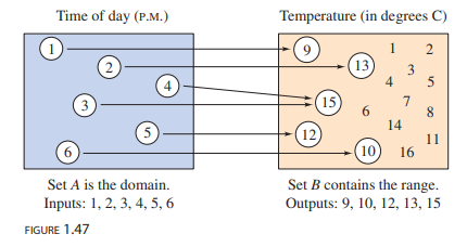
A function $f$ from a set $A$ to a set $B$ is a relation that assigns to each element $x$ in the set $A$ exactly one element $y$ in the set $B$. The set $A$ is the domain (or set of inputs) of the function $f$, and the set $B$ contains the range (or set of outputs).
To help understand this definition, look at the function that relates the time of day to the temperature in Figure 1.47.

This function can be represented by the following ordered pairs, in which the first coordinate ( $x$-value) is the input and the second coordinate ( $y$-value) is the output.
$$
\left{\left(1,9^{\circ}\right),\left(2,13^{\circ}\right),\left(3,15^{\circ}\right),\left(4,15^{\circ}\right),\left(5,12^{\circ}\right),\left(6,10^{\circ}\right)\right}
$$
Characteristics of a Function from Set $A$ to Set $B$

  1. Each element in $A$ must be matched with an element in $B$.
  2. Some elements in $B$ may not be matched with any element in $A$.
  3. Two or more elements in $A$ may be matched with the same element in $B$.
  4. An element in $A$ (the domain) cannot be matched with two different elements in $B$.

数学代写|微积分代写Calculus代写|Function Notation

When an equation is used to represent a function, it is convenient to name the function so that it can be referenced easily. For example, you know that the equation $y=1-x^2$ describes $y$ as a function of $x$. Suppose you give this function the name ” $f$.” Then you can use the following function notation.
$\begin{array}{ccc}\text { Input } & \text { Output } & \text { Equation } \ x & f(x) & f(x)=1-x^2\end{array}$
The symbol $f(x)$ is read as the value of $f$ at $x$ or simply $f$ of $x$. The symbol $f(x)$ corresponds to the $y$-value for a given $x$. So, you can write $y=f(x)$. Keep in mind that $f$ is the name of the function, whereas $f(x)$ is the value of the function at $x$. For instance, the function given by
$$
f(x)=3-2 x
$$
has function values denoted by $f(-1), f(0), f(2)$, and so on. To find these values, substitute the specified input values into the given equation.
$$
\begin{aligned}
\text { For } x & =-1, & f(-1) & =3-2(-1)=3+2=5 . \
& \text { For } x=0, & f(0) & =3-2(0)=3-0=3 . \
\text { For } x & =2, & f(2) & =3-2(2)=3-4=-1 .
\end{aligned}
$$

Although $f$ is often used as a convenient function name and $x$ is often used as the independent variable, you can use other letters. For instance,
$$
f(x)=x^2-4 x+7, \quad f(t)=t^2-4 t+7, \quad \text { and } \quad g(s)=s^2-4 s+7
$$
all define the same function. In fact, the role of the independent variable is that of a “placeholder.” Consequently, the function could be described by
$$
f(\square)=(\square)^2-4(\square)+7 .
$$

数学代写|微积分代写Calculus代写|MTH191

微积分代考

数学代写|微积分代写Calculus代写|Introduction to Functions

许多日常现象涉及两个量,它们通过某种对应规则相互关联。这种对应规则的数学术语是关系。在数学中,关系通常用数学方程和公式来表示。例如,在$\$ 1000$上赚取的1年单利$I$与年利率$r$通过公式$I=1000 \mathrm{r}$相关联。
公式$I=1000 \mathrm{r}$表示一种特殊的关系,它将一个集合中的每个项目与另一个集合中的一个项目进行匹配。这样的关系称为函数。
函数的定义
从集合$A$到集合$B$的函数$f$是一个关系,它将集合$A$中的每个元素$x$精确地分配给集合$B$中的一个元素$y$。集合$A$是函数$f$的域(或一组输入),集合$B$包含范围(或一组输出)。
为了帮助理解这个定义,请看图1.47中将一天中的时间与温度联系起来的函数。

该函数可以用以下有序对表示,其中第一个坐标($x$ -value)是输入,第二个坐标($y$ -value)是输出。
$$
\left{\left(1,9^{\circ}\right),\left(2,13^{\circ}\right),\left(3,15^{\circ}\right),\left(4,15^{\circ}\right),\left(5,12^{\circ}\right),\left(6,10^{\circ}\right)\right}
$$
从集合$A$到集合的函数特征 $B$

$A$中的每个元素必须与$B$中的一个元素匹配。

$B$中的某些元素可能与$A$中的任何元素不匹配。

$A$中的两个或多个元素可以与$B$中的相同元素匹配。

$A$(域)中的一个元素不能与$B$中的两个不同元素匹配。

数学代写|微积分代写Calculus代写|Function Notation

当用一个方程来表示一个函数时,给函数命名是很方便的,这样就可以很容易地引用它。例如,您知道方程$y=1-x^2$将$y$描述为$x$的函数。假设您将此函数命名为“$f$”,那么您可以使用以下函数表示法。
$\begin{array}{ccc}\text { Input } & \text { Output } & \text { Equation } \ x & f(x) & f(x)=1-x^2\end{array}$
符号$f(x)$读取为$f$在$x$处的值,或者直接读取为$x$的$f$。符号$f(x)$对应于给定$x$的$y$ -值。你可以写$y=f(x)$。请记住,$f$是函数的名称,而$f(x)$是函数在$x$处的值。例如,函数由
$$
f(x)=3-2 x
$$
具有用$f(-1), f(0), f(2)$表示的函数值,等等。要找到这些值,将指定的输入值代入给定的方程。
$$
\begin{aligned}
\text { For } x & =-1, & f(-1) & =3-2(-1)=3+2=5 . \
& \text { For } x=0, & f(0) & =3-2(0)=3-0=3 . \
\text { For } x & =2, & f(2) & =3-2(2)=3-4=-1 .
\end{aligned}
$$

虽然$f$常被用作方便的函数名,$x$常被用作自变量,但您也可以使用其他字母。例如,
$$
f(x)=x^2-4 x+7, \quad f(t)=t^2-4 t+7, \quad \text { and } \quad g(s)=s^2-4 s+7
$$
都定义了相同的函数。事实上,自变量的作用是“占位符”。因此,函数可以用
$$
f(\square)=(\square)^2-4(\square)+7 .
$$

数学代写|微积分代写Calculus代写 请认准statistics-lab™

统计代写请认准statistics-lab™. statistics-lab™为您的留学生涯保驾护航。

微观经济学代写

微观经济学是主流经济学的一个分支,研究个人和企业在做出有关稀缺资源分配的决策时的行为以及这些个人和企业之间的相互作用。my-assignmentexpert™ 为您的留学生涯保驾护航 在数学Mathematics作业代写方面已经树立了自己的口碑, 保证靠谱, 高质且原创的数学Mathematics代写服务。我们的专家在图论代写Graph Theory代写方面经验极为丰富,各种图论代写Graph Theory相关的作业也就用不着 说。

线性代数代写

线性代数是数学的一个分支,涉及线性方程,如:线性图,如:以及它们在向量空间和通过矩阵的表示。线性代数是几乎所有数学领域的核心。

博弈论代写

现代博弈论始于约翰-冯-诺伊曼(John von Neumann)提出的两人零和博弈中的混合策略均衡的观点及其证明。冯-诺依曼的原始证明使用了关于连续映射到紧凑凸集的布劳威尔定点定理,这成为博弈论和数学经济学的标准方法。在他的论文之后,1944年,他与奥斯卡-莫根斯特恩(Oskar Morgenstern)共同撰写了《游戏和经济行为理论》一书,该书考虑了几个参与者的合作游戏。这本书的第二版提供了预期效用的公理理论,使数理统计学家和经济学家能够处理不确定性下的决策。

微积分代写

微积分,最初被称为无穷小微积分或 “无穷小的微积分”,是对连续变化的数学研究,就像几何学是对形状的研究,而代数是对算术运算的概括研究一样。

它有两个主要分支,微分和积分;微分涉及瞬时变化率和曲线的斜率,而积分涉及数量的累积,以及曲线下或曲线之间的面积。这两个分支通过微积分的基本定理相互联系,它们利用了无限序列和无限级数收敛到一个明确定义的极限的基本概念 。

计量经济学代写

什么是计量经济学?
计量经济学是统计学和数学模型的定量应用,使用数据来发展理论或测试经济学中的现有假设,并根据历史数据预测未来趋势。它对现实世界的数据进行统计试验,然后将结果与被测试的理论进行比较和对比。

根据你是对测试现有理论感兴趣,还是对利用现有数据在这些观察的基础上提出新的假设感兴趣,计量经济学可以细分为两大类:理论和应用。那些经常从事这种实践的人通常被称为计量经济学家。

Matlab代写

MATLAB 是一种用于技术计算的高性能语言。它将计算、可视化和编程集成在一个易于使用的环境中,其中问题和解决方案以熟悉的数学符号表示。典型用途包括:数学和计算算法开发建模、仿真和原型制作数据分析、探索和可视化科学和工程图形应用程序开发,包括图形用户界面构建MATLAB 是一个交互式系统,其基本数据元素是一个不需要维度的数组。这使您可以解决许多技术计算问题,尤其是那些具有矩阵和向量公式的问题,而只需用 C 或 Fortran 等标量非交互式语言编写程序所需的时间的一小部分。MATLAB 名称代表矩阵实验室。MATLAB 最初的编写目的是提供对由 LINPACK 和 EISPACK 项目开发的矩阵软件的轻松访问,这两个项目共同代表了矩阵计算软件的最新技术。MATLAB 经过多年的发展,得到了许多用户的投入。在大学环境中,它是数学、工程和科学入门和高级课程的标准教学工具。在工业领域,MATLAB 是高效研究、开发和分析的首选工具。MATLAB 具有一系列称为工具箱的特定于应用程序的解决方案。对于大多数 MATLAB 用户来说非常重要,工具箱允许您学习应用专业技术。工具箱是 MATLAB 函数(M 文件)的综合集合,可扩展 MATLAB 环境以解决特定类别的问题。可用工具箱的领域包括信号处理、控制系统、神经网络、模糊逻辑、小波、仿真等。

R语言代写问卷设计与分析代写
PYTHON代写回归分析与线性模型代写
MATLAB代写方差分析与试验设计代写
STATA代写机器学习/统计学习代写
SPSS代写计量经济学代写
EVIEWS代写时间序列分析代写
EXCEL代写深度学习代写
SQL代写各种数据建模与可视化代写

数学代写|微积分代写Calculus代写|MATH1141

如果你也在 怎样代写微积分Calculus 这个学科遇到相关的难题,请随时右上角联系我们的24/7代写客服。微积分Calculus 基本上就是非常高级的代数和几何。从某种意义上说,它甚至不是一门新学科——它采用代数和几何的普通规则,并对它们进行调整,以便它们可以用于更复杂的问题。(当然,问题在于,从另一种意义上说,这是一门新的、更困难的学科。)

微积分Calculus数学之所以有效,是因为曲线在局部是直的;换句话说,它们在微观层面上是直的。地球是圆的,但对我们来说,它看起来是平的,因为与地球的大小相比,我们在微观层面上。微积分之所以有用,是因为当你放大曲线,曲线变直时,你可以用正则代数和几何来处理它们。这种放大过程是通过极限数学来实现的。

statistics-lab™ 为您的留学生涯保驾护航 在代写微积分Calculus方面已经树立了自己的口碑, 保证靠谱, 高质且原创的统计Statistics代写服务。我们的专家在代写微积分Calculus代写方面经验极为丰富,各种代写微积分Calculus相关的作业也就用不着说。

数学代写|微积分代写Calculus代写|MATH1141

数学代写|微积分代写Calculus代写|Linear Equations in Two Variables

The simplest mathematical model for relating two variables is the linear equation in two variables $y=m x+b$. The equation is called linear because its graph is a line. (In mathematics, the term line means straight line.) By letting $x=0$, you can see that the line crosses the $y$-axis at $y=b$, as shown in Figure 1.28. In other words, the $y$-intercept is $(0, b)$. The steepness or slope of the line is $m$.
$$
y=m x+b
$$
The slope of a nonvertical line is the number of units the line rises (or falls) vertically for each unit of horizontal change from left to right, as shown in Figure 1.28 and Figure 1.29.

A linear equation that is written in the form $y=m x+b$ is said to be written in slope-intercept form.
The Slope-Intercept Form of the Equation of a Line
The graph of the equation
$$
y=m x+b
$$
is a line whose slope is $m$ and whose $y$-intercept is $(0, b)$.
Exploration
Use a graphing utility to compare the slopes of the lines $y=m x$, where $m=0.5,1,2$, and 4 . Which line rises most quickly? Now, let $m=-0.5$, $-1,-2$, and -4 . Which line falls most quickly? Use a square setting to obtain a true geometric perspective. What can you conclude about the slope and the “rate” at which the line rises or falls?

Once you have determined the slope and the $y$-intercept of a line, it is a relatively simple matter to sketch its graph. In the next example, note that none of the lines is vertical. A vertical line has an equation of the form
$$
x=a .
$$
Vertical line
The equation of a vertical line cannot be written in the form $y=m x+b$ because the slope of a vertical line is undefined, as indicated in Figure 1.30.

数学代写|微积分代写Calculus代写|Writing Linear Equations in Two Variables

If $\left(x_1, y_1\right)$ is a point on a line of slope $m$ and $(x, y)$ is any other point on the line, then
$$
\frac{y-y_1}{x-x_1}=m .
$$
This equation, involving the variables $x$ and $y$, can be rewritten in the form
$$
y-y_1=m\left(x-x_1\right)
$$
which is the point-slope form of the equation of a line.
Point-Slope Form of the Equation of a Line
The equation of the line with slope $m$ passing through the point $\left(x_1, y_1\right)$ is
$$
y-y_1=m\left(x-x_1\right) .
$$
The point-slope form is most useful for finding the equation of a line. You should remember this form.
Example 3 Using the Point-Slope Form
Find the slope-intercept form of the equation of the line that has a slope of 3 and passes through the point $(1,-2)$.
Solution
Use the point-slope form with $m=3$ and $\left(x_1, y_1\right)=(1,-2)$.
$$
\begin{aligned}
y-y_1 & =m\left(x-x_1\right) & & \text { Point-slope form } \
y-(-2) & =3(x-1) & & \text { Substitute for } m, x_1, \text { and } y_1 . \
y+2 & =3 x-3 & & \text { Simplify. } \
y & =3 x-5 & & \text { Write in slope-intercept form. }
\end{aligned}
$$
The slope-intercept form of the equation of the line is $y=3 x-5$. The graph of this line is shown in Figure 1.39.

数学代写|微积分代写Calculus代写|MATH1141

微积分代考

数学代写|微积分代写Calculus代写|Linear Equations in Two Variables

关系两个变量的最简单的数学模型是两个变量的线性方程$y=m x+b$。这个方程被称为线性方程,因为它的图形是一条直线。(在数学中,“线”一词的意思是直线。)通过设置$x=0$,您可以看到这条线在$y=b$处穿过$y$ -轴,如图1.28所示。也就是说,$y$截距等于$(0, b)$。直线的陡度或斜率为$m$。
$$
y=m x+b
$$
非垂直线的斜率是直线从左向右每发生一个单位的水平变化,直线垂直上升(或下降)的单位数,如图1.28和图1.29所示。

表示为$y=m x+b$的线性方程被称为斜率-截距式。
直线方程的斜截式
方程的图形
$$
y=m x+b
$$
是一条斜率为$m$, $y$截距为$(0, b)$的直线。
探索
使用绘图工具来比较直线$y=m x$的斜率,其中$m=0.5,1,2$和4。哪条线上升最快?现在,让$m=-0.5$$-1,-2$和-4。哪条线掉得最快?使用正方形设置来获得真正的几何透视。关于斜率和直线上升或下降的“速率”,你能得出什么结论?

一旦确定了直线的斜率和$y$ -截距,绘制其图形就相对简单了。在下一个示例中,请注意没有一条线是垂直的。一条垂直线的方程是这样的
$$
x=a .
$$
垂直线
垂直线的方程不能写成$y=m x+b$的形式,因为垂直线的斜率没有定义,如图1.30所示。

数学代写|微积分代写Calculus代写|Writing Linear Equations in Two Variables

如果$\left(x_1, y_1\right)$是斜率为$m$的直线上的一点$(x, y)$是直线上的任意一点,则
$$
\frac{y-y_1}{x-x_1}=m .
$$
这个方程,包含变量$x$和$y$,可以重写为
$$
y-y_1=m\left(x-x_1\right)
$$
也就是直线方程的点斜式。
直线方程的点斜式
斜率为$m$的直线经过点$\left(x_1, y_1\right)$的方程为
$$
y-y_1=m\left(x-x_1\right) .
$$
点斜式在求直线方程时是最有用的。你应该记住这个表格。
例3点斜式的使用
求斜率为3且经过$(1,-2)$点的直线的斜截式方程。
解决方案
使用点斜形式与$m=3$和$\left(x_1, y_1\right)=(1,-2)$。
$$
\begin{aligned}
y-y_1 & =m\left(x-x_1\right) & & \text { Point-slope form } \
y-(-2) & =3(x-1) & & \text { Substitute for } m, x_1, \text { and } y_1 . \
y+2 & =3 x-3 & & \text { Simplify. } \
y & =3 x-5 & & \text { Write in slope-intercept form. }
\end{aligned}
$$
直线方程的斜截式是$y=3 x-5$。该线的曲线图如图1.39所示。

数学代写|微积分代写Calculus代写 请认准statistics-lab™

统计代写请认准statistics-lab™. statistics-lab™为您的留学生涯保驾护航。

微观经济学代写

微观经济学是主流经济学的一个分支,研究个人和企业在做出有关稀缺资源分配的决策时的行为以及这些个人和企业之间的相互作用。my-assignmentexpert™ 为您的留学生涯保驾护航 在数学Mathematics作业代写方面已经树立了自己的口碑, 保证靠谱, 高质且原创的数学Mathematics代写服务。我们的专家在图论代写Graph Theory代写方面经验极为丰富,各种图论代写Graph Theory相关的作业也就用不着 说。

线性代数代写

线性代数是数学的一个分支,涉及线性方程,如:线性图,如:以及它们在向量空间和通过矩阵的表示。线性代数是几乎所有数学领域的核心。

博弈论代写

现代博弈论始于约翰-冯-诺伊曼(John von Neumann)提出的两人零和博弈中的混合策略均衡的观点及其证明。冯-诺依曼的原始证明使用了关于连续映射到紧凑凸集的布劳威尔定点定理,这成为博弈论和数学经济学的标准方法。在他的论文之后,1944年,他与奥斯卡-莫根斯特恩(Oskar Morgenstern)共同撰写了《游戏和经济行为理论》一书,该书考虑了几个参与者的合作游戏。这本书的第二版提供了预期效用的公理理论,使数理统计学家和经济学家能够处理不确定性下的决策。

微积分代写

微积分,最初被称为无穷小微积分或 “无穷小的微积分”,是对连续变化的数学研究,就像几何学是对形状的研究,而代数是对算术运算的概括研究一样。

它有两个主要分支,微分和积分;微分涉及瞬时变化率和曲线的斜率,而积分涉及数量的累积,以及曲线下或曲线之间的面积。这两个分支通过微积分的基本定理相互联系,它们利用了无限序列和无限级数收敛到一个明确定义的极限的基本概念 。

计量经济学代写

什么是计量经济学?
计量经济学是统计学和数学模型的定量应用,使用数据来发展理论或测试经济学中的现有假设,并根据历史数据预测未来趋势。它对现实世界的数据进行统计试验,然后将结果与被测试的理论进行比较和对比。

根据你是对测试现有理论感兴趣,还是对利用现有数据在这些观察的基础上提出新的假设感兴趣,计量经济学可以细分为两大类:理论和应用。那些经常从事这种实践的人通常被称为计量经济学家。

Matlab代写

MATLAB 是一种用于技术计算的高性能语言。它将计算、可视化和编程集成在一个易于使用的环境中,其中问题和解决方案以熟悉的数学符号表示。典型用途包括:数学和计算算法开发建模、仿真和原型制作数据分析、探索和可视化科学和工程图形应用程序开发,包括图形用户界面构建MATLAB 是一个交互式系统,其基本数据元素是一个不需要维度的数组。这使您可以解决许多技术计算问题,尤其是那些具有矩阵和向量公式的问题,而只需用 C 或 Fortran 等标量非交互式语言编写程序所需的时间的一小部分。MATLAB 名称代表矩阵实验室。MATLAB 最初的编写目的是提供对由 LINPACK 和 EISPACK 项目开发的矩阵软件的轻松访问,这两个项目共同代表了矩阵计算软件的最新技术。MATLAB 经过多年的发展,得到了许多用户的投入。在大学环境中,它是数学、工程和科学入门和高级课程的标准教学工具。在工业领域,MATLAB 是高效研究、开发和分析的首选工具。MATLAB 具有一系列称为工具箱的特定于应用程序的解决方案。对于大多数 MATLAB 用户来说非常重要,工具箱允许您学习应用专业技术。工具箱是 MATLAB 函数(M 文件)的综合集合,可扩展 MATLAB 环境以解决特定类别的问题。可用工具箱的领域包括信号处理、控制系统、神经网络、模糊逻辑、小波、仿真等。

R语言代写问卷设计与分析代写
PYTHON代写回归分析与线性模型代写
MATLAB代写方差分析与试验设计代写
STATA代写机器学习/统计学习代写
SPSS代写计量经济学代写
EVIEWS代写时间序列分析代写
EXCEL代写深度学习代写
SQL代写各种数据建模与可视化代写

物理代写|量子场论代写Quantum field theory代考|PHYC90008

如果你也在 怎样代写量子场论Quantum field theory 这个学科遇到相关的难题,请随时右上角联系我们的24/7代写客服。量子场论Quantum field theory提供了一套极其强大的计算方法,但尚未发现任何基本限制。它导致了科学史上理论预测和实验数据之间最奇妙的一致。

量子场论Quantum field theory对我们的宇宙的本质,以及其他可能的自洽宇宙的本质,提供了深刻而深刻的见解。另一方面,这个主题是一团糟。它的基础是脆弱的,它可能是荒谬的复杂,而且很可能是不完整的。通常有很多方法可以解决同样的问题,有时没有一个是特别令人满意的。这给这个主题的介绍的设计和呈现留下了巨大的挑战。

statistics-lab™ 为您的留学生涯保驾护航 在代写量子场论Quantum field theory方面已经树立了自己的口碑, 保证靠谱, 高质且原创的统计Statistics代写服务。我们的专家在代写量子场论Quantum field theory代写方面经验极为丰富,各种代写量子场论Quantum field theory相关的作业也就用不着说。

物理代写|量子场论代写Quantum field theory代考|PHYC90008

物理代写|量子场论代写Quantum field theory代考|Classical electrodynamics

We would expect the Hamiltonian of a system of moving charges, such as an atom, in an electromagnetic field to consist of three parts: a part referring to matter (i.e. the charges), a part referring to the electromagnetic field and a part describing the interaction between matter and field.

For a system of point masses $m_i, i=1, \ldots, N$, with charges $e_i$ and position coordinates $\mathbf{r}i$, the Hamiltonian is $$ H{\mathrm{m}}=\sum_i \frac{\mathbf{p}i^2}{2 m_i}+H{\mathrm{C}}
$$
where $H_{\mathrm{C}}$ is the Coulomb interaction
$$
H_{\mathrm{C}} \equiv \frac{1}{2} \sum_{\substack{i, j \(i \neq j)}} \frac{e_i e_j}{4 \pi\left|\mathbf{r}_i-\mathbf{r}_j\right|}
$$
and $\mathbf{p}_i=m_i \mathrm{~d} \mathbf{r}_i / \mathrm{d} t$ is the kinetic momentum of the $i$ th particle. This is the usual Hamiltonian of atomic physics, for example.

The electromagnetic field in interaction with charges is described by Maxwell’s equations [Eqs. (1.1)]. We continue to use the Coulomb gauge, $\boldsymbol{\nabla} \cdot \mathbf{A}=0$, so that the electric field (1.2) decomposes into transverse and longitudinal fields
$$
\mathbf{E}=\mathbf{E}{\mathbf{T}}+\mathbf{E}{\mathbf{L}},
$$
where
$$
\mathbf{E}{\mathbf{T}}=-\frac{1}{c} \frac{\partial \mathbf{A}}{\partial t}, \quad \mathbf{E}{\mathbf{L}}=-\nabla \phi
$$

物理代写|量子场论代写Quantum field theory代考|Quantum electrodynamics

The quantization of the system described by the Hamiltonian (1.63) is carried out by subjecting the particles’ coordinates $\mathbf{r}i$ and canonically conjugate momenta $\mathbf{p}_i$ to the usual commutation relations (e.g. in the coordinate representation $\mathbf{p}_i \rightarrow i \hbar \boldsymbol{\nabla}_i$ ), and quantizing the radiation field, as in Section 1.2.3. The longitudinal electric field $\mathbf{E}{\mathbf{L}}$ does not pro

The eigenstates of $H_0$ are again of the form
$$
\left|A, \ldots n_r(\mathbf{k}) \ldots\right\rangle=|A\rangle\left|\ldots n_r(\mathbf{k}) \ldots\right\rangle,
$$
with $|A\rangle$ and $\left|\ldots n_r(\mathbf{k}) \ldots\right\rangle$ eigenstates of $H_{\mathrm{m}}$ and $H_{\mathrm{rad}}$.
Compared with the electric dipole interaction (1.40), the interaction (1.62) differs in that it contains a term quadratic in the vector potential. This results in two-photon processes in first-order perturbation theory (i.e. emission or absorption of two photons or scattering). In addition, the first term in (1.62) contains magnetic interactions and higher-order effects due to the spatial variation of $\mathbf{A}(\mathbf{x}, t)$, which are absent from the electric dipole interaction (1.40). These aspects are illustrated in the applications to radiative transitions and Thomson scattering which follow.

vide any additional degrees of freedom, being completely determined via the first Maxwell equation $\boldsymbol{\nabla} \cdot \mathbf{E}_{\mathbf{L}}=\rho$ by the charges.

The interaction $H_{\mathrm{I}}$ in Eq, (1.63) is usually treated as a perturbation which causes transitions between the states of the non-interacting Hamiltonian
$$
H_0=H_{\mathrm{m}}+H_{\text {rad }} \text {. }
$$

物理代写|量子场论代写Quantum field theory代考|PHYC90008

量子场论代考

物理代写|量子场论代写Quantum field theory代考|Classical electrodynamics

我们期望在电磁场中运动电荷系统(如原子)的哈密顿量由三部分组成:一部分涉及物质(即电荷),一部分涉及电磁场,另一部分描述物质与场之间的相互作用。

对于质点系统$m_i, i=1, \ldots, N$,电荷为$e_i$,位置坐标为$\mathbf{r}i$,哈密顿量为$$ H{\mathrm{m}}=\sum_i \frac{\mathbf{p}i^2}{2 m_i}+H{\mathrm{C}}
$$
库仑相互作用$H_{\mathrm{C}}$在哪里
$$
H_{\mathrm{C}} \equiv \frac{1}{2} \sum_{\substack{i, j (i \neq j)}} \frac{e_i e_j}{4 \pi\left|\mathbf{r}_i-\mathbf{r}_j\right|}
$$
$\mathbf{p}_i=m_i \mathrm{~d} \mathbf{r}_i / \mathrm{d} t$是第$i$个粒子的动能。例如,这是原子物理学中常用的哈密顿量。

电磁场与电荷的相互作用用麦克斯韦方程描述。(1.1)]。我们继续使用库仑规$\boldsymbol{\nabla} \cdot \mathbf{A}=0$,使电场(1.2)分解为横向场和纵向场
$$
\mathbf{E}=\mathbf{E}{\mathbf{T}}+\mathbf{E}{\mathbf{L}},
$$
在哪里
$$
\mathbf{E}{\mathbf{T}}=-\frac{1}{c} \frac{\partial \mathbf{A}}{\partial t}, \quad \mathbf{E}{\mathbf{L}}=-\nabla \phi
$$

物理代写|量子场论代写Quantum field theory代考|Quantum electrodynamics

由哈密顿量(1.63)描述的系统的量子化是通过使粒子的坐标$\mathbf{r}i$和标准共轭动量$\mathbf{p}_i$服从通常的对易关系(例如在坐标表示$\mathbf{p}_i \rightarrow i \hbar \boldsymbol{\nabla}_i$中),并将辐射场量子化来实现的,如第1.2.3节所述。纵向电场$\mathbf{E}{\mathbf{L}}$不亲

$H_0$的特征态也是这种形式
$$
\left|A, \ldots n_r(\mathbf{k}) \ldots\right\rangle=|A\rangle\left|\ldots n_r(\mathbf{k}) \ldots\right\rangle,
$$
具有$|A\rangle$和$\left|\ldots n_r(\mathbf{k}) \ldots\right\rangle$的特征态$H_{\mathrm{m}}$和$H_{\mathrm{rad}}$。
与电偶极相互作用(1.40)相比,相互作用(1.62)的不同之处在于它在矢量势中包含了一个二次项。这导致了一阶微扰理论中的双光子过程(即两个光子的发射或吸收或散射)。此外,(1.62)中的第一项包含磁相互作用和高阶效应,这是由于$\mathbf{A}(\mathbf{x}, t)$的空间变化,这在电偶极相互作用(1.40)中不存在。这些方面将在随后的辐射跃迁和汤姆逊散射的应用中加以说明。

没有任何额外的自由度,完全由第一个麦克斯韦方程$\boldsymbol{\nabla} \cdot \mathbf{E}_{\mathbf{L}}=\rho$由电荷决定。

Eq,(1.63)中的相互作用$H_{\mathrm{I}}$通常被视为引起非相互作用哈密顿量状态之间转换的扰动
$$
H_0=H_{\mathrm{m}}+H_{\text {rad }} \text {. }
$$

物理代写|量子场论代写Quantum field theory代考 请认准statistics-lab™

统计代写请认准statistics-lab™. statistics-lab™为您的留学生涯保驾护航。

金融工程代写

金融工程是使用数学技术来解决金融问题。金融工程使用计算机科学、统计学、经济学和应用数学领域的工具和知识来解决当前的金融问题,以及设计新的和创新的金融产品。

非参数统计代写

非参数统计指的是一种统计方法,其中不假设数据来自于由少数参数决定的规定模型;这种模型的例子包括正态分布模型和线性回归模型。

广义线性模型代考

广义线性模型(GLM)归属统计学领域,是一种应用灵活的线性回归模型。该模型允许因变量的偏差分布有除了正态分布之外的其它分布。

术语 广义线性模型(GLM)通常是指给定连续和/或分类预测因素的连续响应变量的常规线性回归模型。它包括多元线性回归,以及方差分析和方差分析(仅含固定效应)。

有限元方法代写

有限元方法(FEM)是一种流行的方法,用于数值解决工程和数学建模中出现的微分方程。典型的问题领域包括结构分析、传热、流体流动、质量运输和电磁势等传统领域。

有限元是一种通用的数值方法,用于解决两个或三个空间变量的偏微分方程(即一些边界值问题)。为了解决一个问题,有限元将一个大系统细分为更小、更简单的部分,称为有限元。这是通过在空间维度上的特定空间离散化来实现的,它是通过构建对象的网格来实现的:用于求解的数值域,它有有限数量的点。边界值问题的有限元方法表述最终导致一个代数方程组。该方法在域上对未知函数进行逼近。[1] 然后将模拟这些有限元的简单方程组合成一个更大的方程系统,以模拟整个问题。然后,有限元通过变化微积分使相关的误差函数最小化来逼近一个解决方案。

tatistics-lab作为专业的留学生服务机构,多年来已为美国、英国、加拿大、澳洲等留学热门地的学生提供专业的学术服务,包括但不限于Essay代写,Assignment代写,Dissertation代写,Report代写,小组作业代写,Proposal代写,Paper代写,Presentation代写,计算机作业代写,论文修改和润色,网课代做,exam代考等等。写作范围涵盖高中,本科,研究生等海外留学全阶段,辐射金融,经济学,会计学,审计学,管理学等全球99%专业科目。写作团队既有专业英语母语作者,也有海外名校硕博留学生,每位写作老师都拥有过硬的语言能力,专业的学科背景和学术写作经验。我们承诺100%原创,100%专业,100%准时,100%满意。

随机分析代写


随机微积分是数学的一个分支,对随机过程进行操作。它允许为随机过程的积分定义一个关于随机过程的一致的积分理论。这个领域是由日本数学家伊藤清在第二次世界大战期间创建并开始的。

时间序列分析代写

随机过程,是依赖于参数的一组随机变量的全体,参数通常是时间。 随机变量是随机现象的数量表现,其时间序列是一组按照时间发生先后顺序进行排列的数据点序列。通常一组时间序列的时间间隔为一恒定值(如1秒,5分钟,12小时,7天,1年),因此时间序列可以作为离散时间数据进行分析处理。研究时间序列数据的意义在于现实中,往往需要研究某个事物其随时间发展变化的规律。这就需要通过研究该事物过去发展的历史记录,以得到其自身发展的规律。

回归分析代写

多元回归分析渐进(Multiple Regression Analysis Asymptotics)属于计量经济学领域,主要是一种数学上的统计分析方法,可以分析复杂情况下各影响因素的数学关系,在自然科学、社会和经济学等多个领域内应用广泛。

MATLAB代写

MATLAB 是一种用于技术计算的高性能语言。它将计算、可视化和编程集成在一个易于使用的环境中,其中问题和解决方案以熟悉的数学符号表示。典型用途包括:数学和计算算法开发建模、仿真和原型制作数据分析、探索和可视化科学和工程图形应用程序开发,包括图形用户界面构建MATLAB 是一个交互式系统,其基本数据元素是一个不需要维度的数组。这使您可以解决许多技术计算问题,尤其是那些具有矩阵和向量公式的问题,而只需用 C 或 Fortran 等标量非交互式语言编写程序所需的时间的一小部分。MATLAB 名称代表矩阵实验室。MATLAB 最初的编写目的是提供对由 LINPACK 和 EISPACK 项目开发的矩阵软件的轻松访问,这两个项目共同代表了矩阵计算软件的最新技术。MATLAB 经过多年的发展,得到了许多用户的投入。在大学环境中,它是数学、工程和科学入门和高级课程的标准教学工具。在工业领域,MATLAB 是高效研究、开发和分析的首选工具。MATLAB 具有一系列称为工具箱的特定于应用程序的解决方案。对于大多数 MATLAB 用户来说非常重要,工具箱允许您学习应用专业技术。工具箱是 MATLAB 函数(M 文件)的综合集合,可扩展 MATLAB 环境以解决特定类别的问题。可用工具箱的领域包括信号处理、控制系统、神经网络、模糊逻辑、小波、仿真等。

R语言代写问卷设计与分析代写
PYTHON代写回归分析与线性模型代写
MATLAB代写方差分析与试验设计代写
STATA代写机器学习/统计学习代写
SPSS代写计量经济学代写
EVIEWS代写时间序列分析代写
EXCEL代写深度学习代写
SQL代写各种数据建模与可视化代写

物理代写|量子场论代写Quantum field theory代考|PHYS4125

如果你也在 怎样代写量子场论Quantum field theory 这个学科遇到相关的难题,请随时右上角联系我们的24/7代写客服。量子场论Quantum field theory提供了一套极其强大的计算方法,但尚未发现任何基本限制。它导致了科学史上理论预测和实验数据之间最奇妙的一致。

量子场论Quantum field theory对我们的宇宙的本质,以及其他可能的自洽宇宙的本质,提供了深刻而深刻的见解。另一方面,这个主题是一团糟。它的基础是脆弱的,它可能是荒谬的复杂,而且很可能是不完整的。通常有很多方法可以解决同样的问题,有时没有一个是特别令人满意的。这给这个主题的介绍的设计和呈现留下了巨大的挑战。

statistics-lab™ 为您的留学生涯保驾护航 在代写量子场论Quantum field theory方面已经树立了自己的口碑, 保证靠谱, 高质且原创的统计Statistics代写服务。我们的专家在代写量子场论Quantum field theory代写方面经验极为丰富,各种代写量子场论Quantum field theory相关的作业也就用不着说。

物理代写|量子场论代写Quantum field theory代考|PHYS4125

物理代写|量子场论代写Quantum field theory代考|The quantized radiation field

The harmonic oscillator results we have derived can at once be applied to the radiation field. Its Hamiltonian, Eq. (1.18), is a superposition of independent harmonic oscillator Hamiltonians (1.20), one for each mode of the radiation field. [The order of the factors in (1.18) is not significant and can be changed, since the $a_{\mathrm{r}}$ and $a_r^*$ are classical amplitudes.] We therefore introduce commutation relations analogous to Eq. (1.19)
$$
\left.\begin{array}{l}
{\left[a_r(\mathbf{k}), a_s^{\dagger}\left(\mathbf{k}^{\prime}\right)\right]=\delta_{r s} \delta_{\mathbf{k} \mathbf{k}^{\prime}}} \
{\left[a_r(\mathbf{k}), a_s\left(\mathbf{k}^{\prime}\right)\right]=\left[a_r^{\dagger}(\mathbf{k}), a_s^{\dagger}\left(\mathbf{k}^{\prime}\right)\right]=0}
\end{array}\right}
$$
and write the Hamiltonian (1.18) as
$$
H_{\mathrm{rad}}=\sum_{\mathbf{k}} \sum_r \hbar \omega_{\mathbf{k}}\left(a_r^{\dagger}(\mathbf{k}) a_r(\mathbf{k})+\frac{1}{2}\right) .
$$
The operators
$$
N_r(\mathbf{k})=a_r^{\dagger}(\mathbf{k}) a_r(\mathbf{k})
$$
then have eigenvalues $n_r(\mathbf{k})=0,1,2, \ldots$, and eigenfunctions of the form (1.25)
$$
\left|n_r(\mathbf{k})\right\rangle=\frac{\left[a_r^{\dagger}(\mathbf{k})\right]^{n_r(\mathbf{k})}}{\sqrt{n_r(\mathbf{k}) !}}|0\rangle .
$$
The eigenfunctions of the radiation Hamiltonian (1.30) are products of such states, i.e.
$$
\left|\ldots n_r(\mathbf{k}) \ldots\right\rangle=\prod_{\mathbf{k}i} \prod{r_i}\left|n_{r_i}\left(\mathbf{k}i\right)\right\rangle $$ with energy $$ \sum{\mathbf{k}} \sum_r \hbar \omega_{\mathbf{k}}\left(n_r(\mathbf{k})+\frac{1}{2}\right)
$$

物理代写|量子场论代写Quantum field theory代考|The Electric Dipole Interaction

In the last section we quantized the radiation field. Since the occupation number operators $a_r^{\dagger}(\mathbf{k}) a_r(\mathbf{k})$ commute with the radiation Hamiltonian (1.37), the occupation numbers $n_r(\mathbf{k})$ are constants of the motion for the free field. For anything ‘to happen’ requires interactions with charges and currents so that photons can be absorbed, emitted or scattered.

The complete description of the interaction of a system of charges (for example, an atom or a nucleus) with an electromagnetic field is very complicated. In this section we shall consider the simpler and, in practice, important special case of the interaction occurring via the electric dipole moment of the system of charges. The more complete (but still noncovariant) treatment of Section 1.4 will justify some of the points asserted in this section.
We shall consider a system of $N$ charges $e_1, e_2, \ldots, e_N$ which can be described nonrelativistically, i.e. the position of $\mathrm{e}i, i=1, \ldots, N$, at time $t$ is classically given by $\mathbf{r}_i=\mathbf{r}_i(t)$. We consider transitions between def inite initial and final states of the system (e.g. between two states of an atom). The transitions are brought about by the electric dipole interaction if two approximations are valid. Firstly it is permissible to neglect the interactions with the magnetic field. Secondly, one may neglect the spatial variation of the electric radiation field, causing the transitions, across the system of charges (e.g. across the atom). Under these conditions the electric field $$ \mathbf{E}{\mathrm{T}}(\mathbf{r}, t)=-\frac{1}{c} \frac{\partial \mathbf{A}(\mathbf{r}, t)}{\partial t},
$$
resulting from the transverse vector potential (1.38) of the radiation field (we are again using the Coulomb gauge $\boldsymbol{\nabla} \cdot \mathbf{A}=0$ ), can be calculated at one point somewhere inside the system of charges, instead of at the position of each charge. ${ }^6$ Taking this point as the origin of coordinates $\mathbf{r}=0$, we obtain for the interaction causing transitions, the electric dipole interaction $H_{\mathrm{I}}$ given by
$$
H_{\mathrm{I}}=-\mathbf{D} \cdot \mathbf{E}_{\mathrm{T}}(0, t)
$$
where the electric dipole moment is defined by
$$
\mathbf{D}=\sum e_i \mathbf{r}_i
$$

物理代写|量子场论代写Quantum field theory代考|PHYS4125

量子场论代考

物理代写|量子场论代写Quantum field theory代考|The quantized radiation field

我们所导出的谐振子结果可以立即应用于辐射领域。它的哈密顿量Eq.(1.18)是独立谐振子哈密顿量(1.20)的叠加,每个模式对应一个辐射场。(1.18)中因子的顺序不显著,可以改变,因为$a_{\mathrm{r}}$和$a_r^*$是经典振幅。因此,我们引入类似于式(1.19)的交换关系。
$$
\left.\begin{array}{l}
{\left[a_r(\mathbf{k}), a_s^{\dagger}\left(\mathbf{k}^{\prime}\right)\right]=\delta_{r s} \delta_{\mathbf{k} \mathbf{k}^{\prime}}} \
{\left[a_r(\mathbf{k}), a_s\left(\mathbf{k}^{\prime}\right)\right]=\left[a_r^{\dagger}(\mathbf{k}), a_s^{\dagger}\left(\mathbf{k}^{\prime}\right)\right]=0}
\end{array}\right}
$$
把哈密顿式(1.18)写成
$$
H_{\mathrm{rad}}=\sum_{\mathbf{k}} \sum_r \hbar \omega_{\mathbf{k}}\left(a_r^{\dagger}(\mathbf{k}) a_r(\mathbf{k})+\frac{1}{2}\right) .
$$
算子
$$
N_r(\mathbf{k})=a_r^{\dagger}(\mathbf{k}) a_r(\mathbf{k})
$$
则有特征值$n_r(\mathbf{k})=0,1,2, \ldots$,特征函数的形式为(1.25)
$$
\left|n_r(\mathbf{k})\right\rangle=\frac{\left[a_r^{\dagger}(\mathbf{k})\right]^{n_r(\mathbf{k})}}{\sqrt{n_r(\mathbf{k}) !}}|0\rangle .
$$
辐射哈密顿量(1.30)的本征函数是这些状态的乘积,即。
$$
\left|\ldots n_r(\mathbf{k}) \ldots\right\rangle=\prod_{\mathbf{k}i} \prod{r_i}\left|n_{r_i}\left(\mathbf{k}i\right)\right\rangle $$ with energy $$ \sum{\mathbf{k}} \sum_r \hbar \omega_{\mathbf{k}}\left(n_r(\mathbf{k})+\frac{1}{2}\right)
$$

物理代写|量子场论代写Quantum field theory代考|The Electric Dipole Interaction

在上一节中,我们对辐射场进行了量子化。由于占用数运算符$a_r^{\dagger}(\mathbf{k}) a_r(\mathbf{k})$与辐射哈密顿量(1.37)互换,因此占用数$n_r(\mathbf{k})$是自由场运动的常数。任何“发生”的事情都需要与电荷和电流相互作用,这样光子才能被吸收、发射或散射。

电荷系统(例如原子或原子核)与电磁场相互作用的完整描述是非常复杂的。在本节中,我们将考虑通过电荷系统的电偶极矩发生的相互作用的更简单、在实践中更重要的特殊情况。对1.4节的更完整(但仍然是非协变的)处理将证明本节中断言的一些观点是正确的。
我们将考虑一个由$N$电荷$e_1, e_2, \ldots, e_N$组成的系统,它可以用非相对论性来描述,即$\mathrm{e}i, i=1, \ldots, N$在时间$t$时的位置经典地由$\mathbf{r}i=\mathbf{r}_i(t)$给出。我们考虑系统的确定初始状态和最终状态之间的转换(例如,在原子的两个状态之间)。如果两个近似都成立,则跃迁是由电偶极相互作用引起的。首先,可以忽略与磁场的相互作用。其次,人们可以忽略电辐射场的空间变化,它会引起整个电荷系统(例如原子)的跃迁。在这些条件下电场$$ \mathbf{E}{\mathrm{T}}(\mathbf{r}, t)=-\frac{1}{c} \frac{\partial \mathbf{A}(\mathbf{r}, t)}{\partial t}, $$ 由辐射场的横向矢量势(1.38)产生(我们再次使用库仑规$\boldsymbol{\nabla} \cdot \mathbf{A}=0$),可以在电荷系统内的某个点计算,而不是在每个电荷的位置。${ }^6$以该点为坐标原点$\mathbf{r}=0$,我们得到引起跃迁的相互作用,电偶极相互作用$H{\mathrm{I}}$由
$$
H_{\mathrm{I}}=-\mathbf{D} \cdot \mathbf{E}_{\mathrm{T}}(0, t)
$$
电偶极矩的定义是什么
$$
\mathbf{D}=\sum e_i \mathbf{r}_i
$$

物理代写|量子场论代写Quantum field theory代考 请认准statistics-lab™

统计代写请认准statistics-lab™. statistics-lab™为您的留学生涯保驾护航。

金融工程代写

金融工程是使用数学技术来解决金融问题。金融工程使用计算机科学、统计学、经济学和应用数学领域的工具和知识来解决当前的金融问题,以及设计新的和创新的金融产品。

非参数统计代写

非参数统计指的是一种统计方法,其中不假设数据来自于由少数参数决定的规定模型;这种模型的例子包括正态分布模型和线性回归模型。

广义线性模型代考

广义线性模型(GLM)归属统计学领域,是一种应用灵活的线性回归模型。该模型允许因变量的偏差分布有除了正态分布之外的其它分布。

术语 广义线性模型(GLM)通常是指给定连续和/或分类预测因素的连续响应变量的常规线性回归模型。它包括多元线性回归,以及方差分析和方差分析(仅含固定效应)。

有限元方法代写

有限元方法(FEM)是一种流行的方法,用于数值解决工程和数学建模中出现的微分方程。典型的问题领域包括结构分析、传热、流体流动、质量运输和电磁势等传统领域。

有限元是一种通用的数值方法,用于解决两个或三个空间变量的偏微分方程(即一些边界值问题)。为了解决一个问题,有限元将一个大系统细分为更小、更简单的部分,称为有限元。这是通过在空间维度上的特定空间离散化来实现的,它是通过构建对象的网格来实现的:用于求解的数值域,它有有限数量的点。边界值问题的有限元方法表述最终导致一个代数方程组。该方法在域上对未知函数进行逼近。[1] 然后将模拟这些有限元的简单方程组合成一个更大的方程系统,以模拟整个问题。然后,有限元通过变化微积分使相关的误差函数最小化来逼近一个解决方案。

tatistics-lab作为专业的留学生服务机构,多年来已为美国、英国、加拿大、澳洲等留学热门地的学生提供专业的学术服务,包括但不限于Essay代写,Assignment代写,Dissertation代写,Report代写,小组作业代写,Proposal代写,Paper代写,Presentation代写,计算机作业代写,论文修改和润色,网课代做,exam代考等等。写作范围涵盖高中,本科,研究生等海外留学全阶段,辐射金融,经济学,会计学,审计学,管理学等全球99%专业科目。写作团队既有专业英语母语作者,也有海外名校硕博留学生,每位写作老师都拥有过硬的语言能力,专业的学科背景和学术写作经验。我们承诺100%原创,100%专业,100%准时,100%满意。

随机分析代写


随机微积分是数学的一个分支,对随机过程进行操作。它允许为随机过程的积分定义一个关于随机过程的一致的积分理论。这个领域是由日本数学家伊藤清在第二次世界大战期间创建并开始的。

时间序列分析代写

随机过程,是依赖于参数的一组随机变量的全体,参数通常是时间。 随机变量是随机现象的数量表现,其时间序列是一组按照时间发生先后顺序进行排列的数据点序列。通常一组时间序列的时间间隔为一恒定值(如1秒,5分钟,12小时,7天,1年),因此时间序列可以作为离散时间数据进行分析处理。研究时间序列数据的意义在于现实中,往往需要研究某个事物其随时间发展变化的规律。这就需要通过研究该事物过去发展的历史记录,以得到其自身发展的规律。

回归分析代写

多元回归分析渐进(Multiple Regression Analysis Asymptotics)属于计量经济学领域,主要是一种数学上的统计分析方法,可以分析复杂情况下各影响因素的数学关系,在自然科学、社会和经济学等多个领域内应用广泛。

MATLAB代写

MATLAB 是一种用于技术计算的高性能语言。它将计算、可视化和编程集成在一个易于使用的环境中,其中问题和解决方案以熟悉的数学符号表示。典型用途包括:数学和计算算法开发建模、仿真和原型制作数据分析、探索和可视化科学和工程图形应用程序开发,包括图形用户界面构建MATLAB 是一个交互式系统,其基本数据元素是一个不需要维度的数组。这使您可以解决许多技术计算问题,尤其是那些具有矩阵和向量公式的问题,而只需用 C 或 Fortran 等标量非交互式语言编写程序所需的时间的一小部分。MATLAB 名称代表矩阵实验室。MATLAB 最初的编写目的是提供对由 LINPACK 和 EISPACK 项目开发的矩阵软件的轻松访问,这两个项目共同代表了矩阵计算软件的最新技术。MATLAB 经过多年的发展,得到了许多用户的投入。在大学环境中,它是数学、工程和科学入门和高级课程的标准教学工具。在工业领域,MATLAB 是高效研究、开发和分析的首选工具。MATLAB 具有一系列称为工具箱的特定于应用程序的解决方案。对于大多数 MATLAB 用户来说非常重要,工具箱允许您学习应用专业技术。工具箱是 MATLAB 函数(M 文件)的综合集合,可扩展 MATLAB 环境以解决特定类别的问题。可用工具箱的领域包括信号处理、控制系统、神经网络、模糊逻辑、小波、仿真等。

R语言代写问卷设计与分析代写
PYTHON代写回归分析与线性模型代写
MATLAB代写方差分析与试验设计代写
STATA代写机器学习/统计学习代写
SPSS代写计量经济学代写
EVIEWS代写时间序列分析代写
EXCEL代写深度学习代写
SQL代写各种数据建模与可视化代写

物理代写|量子场论代写Quantum field theory代考|FYS4170

如果你也在 怎样代写量子场论Quantum field theory 这个学科遇到相关的难题,请随时右上角联系我们的24/7代写客服。量子场论Quantum field theory提供了一套极其强大的计算方法,但尚未发现任何基本限制。它导致了科学史上理论预测和实验数据之间最奇妙的一致。

量子场论Quantum field theory对我们的宇宙的本质,以及其他可能的自洽宇宙的本质,提供了深刻而深刻的见解。另一方面,这个主题是一团糟。它的基础是脆弱的,它可能是荒谬的复杂,而且很可能是不完整的。通常有很多方法可以解决同样的问题,有时没有一个是特别令人满意的。这给这个主题的介绍的设计和呈现留下了巨大的挑战。

statistics-lab™ 为您的留学生涯保驾护航 在代写量子场论Quantum field theory方面已经树立了自己的口碑, 保证靠谱, 高质且原创的统计Statistics代写服务。我们的专家在代写量子场论Quantum field theory代写方面经验极为丰富,各种代写量子场论Quantum field theory相关的作业也就用不着说。

物理代写|量子场论代写Quantum field theory代考|FYS4170

物理代写|量子场论代写Quantum field theory代考|The classical field

Classical electromagnetic theory is summed up in Maxwell’s equations. In the presence of a charge density $\rho(\mathbf{x}, t)$ and a current density $\mathbf{j}(\mathbf{x}, \mathrm{t})$, the electric and magnetic fields $\mathbf{E}$ and $\mathbf{B}$ satisfy the equations
$$
\begin{aligned}
\boldsymbol{\nabla} \cdot \mathbf{E} & =\rho \
\boldsymbol{\nabla} \wedge \mathbf{B} & =\frac{1}{c} \mathbf{j}+\frac{1}{c} \frac{\partial \mathbf{E}}{\partial t} \
\boldsymbol{\nabla} \cdot \mathbf{B} & =0 \
\boldsymbol{\nabla} \wedge \mathbf{E} & =-\frac{1}{c} \frac{\partial \mathbf{B}}{\partial t}
\end{aligned}
$$
where, as throughout this book, rationalized Gaussian (c.g.s.) units are being used. ${ }^1$
From the second pair of Maxwell’s equations [Eqs. (1.1c) and (1.1d)] follows the existence of scalar and vector potentials $\phi(\mathbf{x}, t)$ and $\mathbf{A}(\mathbf{x}, t)$, defined by
$$
\mathbf{B}=\boldsymbol{\nabla} \wedge \mathbf{A}, \quad \mathbf{E}=-\boldsymbol{\nabla} \phi-\frac{1}{c} \frac{\partial \mathbf{A}}{\partial t} .
$$
Eqs. (1.2) do not determine the potentials uniquely, since for an arbitrary function $f(\mathbf{x}, t)$ the transformation
$$
\phi \rightarrow \phi^{\prime}=\phi+\frac{1}{c} \frac{\partial f}{\partial t}, \quad \mathbf{A} \rightarrow \mathbf{A}^{\prime}=\mathbf{A}-\nabla f
$$
leaves the fields $\mathbf{E}$ and $\mathbf{B}$ unaltered. The transformation (1.3) is known as a gauge transformation of the second kind. Since all observable quantities can be expressed in terms of $\mathbf{E}$ and $\mathbf{B}$, it is a fundamental requirement of any theory formulated in terms of potentials that it is gauge-invariant, i.e. that the predictions for observable quantities are invariant under such gauge transformations.

Expressed in terms of the potentials, the second pair of Maxwell’s equations [Eqs. (1.1c) and (1.1d)] are satisfied automatically, while the first pair [Eqs. (1.1a) and (1.1b)] become
$$
\begin{gathered}
-\nabla^2 \phi-\frac{1}{c} \frac{\partial}{\partial t}(\boldsymbol{\nabla} \cdot \mathbf{A})=\square \phi-\frac{1}{c} \frac{\partial}{\partial t}\left(\frac{1}{c} \frac{\partial \phi}{\partial t}+\nabla \cdot \mathbf{A}\right)=\rho \
\square \mathbf{A}+\boldsymbol{\nabla}\left(\frac{1}{c} \frac{\partial \phi}{\partial t}+\nabla \cdot \mathbf{A}\right)=\frac{1}{c} \mathbf{j}
\end{gathered}
$$
where
$$
\square \equiv \frac{1}{c^2} \frac{\partial^2}{\partial t^2}-\nabla^2
$$

物理代写|量子场论代写Quantum field theory代考|Harmonic oscillator

The harmonic oscillator Hamiltonian is, in an obvious notation,
$$
H_{\mathrm{osc}}=\frac{p^2}{2 m}+\frac{1}{2} m \omega^2 q^2,
$$
with $q$ and $p$ satisf ying the commutation relation $[q, p]=\mathrm{i} \hbar$. We introduce the operators
$$
\left.\begin{array}{c}
a \
a^{\dagger}
\end{array}\right}=\frac{1}{(2 \hbar m \omega)^{1 / 2}}(m \omega q \pm \mathrm{i} p) .
$$
These satisfy the commutation relation
$$
\left[a, a^{\dagger}\right]=1,
$$
and the Hamiltonian expressed in terms of $a$ and $a^{\dagger}$ becomes:
$$
H_{\mathrm{osc}}=\frac{1}{2} \hbar \omega\left(a^{\dagger} a+a a^{\dagger}\right)=\hbar \omega\left(a^{\dagger} a+\frac{1}{2}\right) .
$$
This is essentially the operator
$$
N \equiv a^{\dagger} a,
$$

which is positive definite, i.e. for any state $|\Psi\rangle$
$$
\langle\Psi|N| \Psi\rangle=\left\langle\Psi\left|a^{\dagger} a\right| \Psi\right\rangle=\langle a \Psi \mid a \Psi\rangle \geq 0 .
$$
Hence, $N$ possesses a lowest non-negative eigenvalue
$$
\alpha_0 \geq 0 \text {. }
$$
It follows from the eigenvalue equation
$$
N|\alpha\rangle=\alpha|\alpha\rangle
$$
and Eq. (1.19) that
$$
N a|\alpha\rangle=(\alpha-1) a|\alpha\rangle, \quad N a^{\dagger}|\alpha\rangle=(\alpha+1) a^{\dagger}|\alpha\rangle,
$$
i.e. $a|\alpha\rangle$ and $a^{\dagger}|\alpha\rangle$ are eigenfunctions of $N$ belonging to the eigenvalues $(\alpha-1)$ and $(\alpha+1)$, respectively. Since $\alpha_0$ is the lowest eigenvalue we must have
$$
a\left|\alpha_0\right\rangle=0
$$
and since
$$
a^{\dagger} a\left|\alpha_0\right\rangle=\alpha_0\left|\alpha_0\right\rangle
$$
Eq. (1.23) implies $\alpha_0=0$. It follows from Eqs. (1.19) and (1.22) that the eigenvalues of $N$ are the integers $n=0,1,2, \ldots$, and that if $\langle n \mid n\rangle=1$, then the states $|n \pm 1\rangle$, defined by
$$
a|n\rangle=n^{1 / 2}|n-1\rangle, \quad a^{\dagger}|n\rangle=(n+1)^{1 / 2}|n+1\rangle,
$$
are also normed to unity. If $\langle 0 \mid 0\rangle=1$, the normed eigenf unctions of $N$ are
$$
|n\rangle=\frac{\left(a^{\dagger}\right)^n}{\sqrt{n !}}|0\rangle, \quad n=0,1,2, \ldots
$$

物理代写|量子场论代写Quantum field theory代考|FYS4170

量子场论代考

物理代写|量子场论代写Quantum field theory代考|The classical field

经典电磁理论可归纳为麦克斯韦方程组。当电荷密度$\rho(\mathbf{x}, t)$和电流密度$\mathbf{j}(\mathbf{x}, \mathrm{t})$存在时,电场$\mathbf{E}$和磁场$\mathbf{B}$满足方程
$$
\begin{aligned}
\boldsymbol{\nabla} \cdot \mathbf{E} & =\rho \
\boldsymbol{\nabla} \wedge \mathbf{B} & =\frac{1}{c} \mathbf{j}+\frac{1}{c} \frac{\partial \mathbf{E}}{\partial t} \
\boldsymbol{\nabla} \cdot \mathbf{B} & =0 \
\boldsymbol{\nabla} \wedge \mathbf{E} & =-\frac{1}{c} \frac{\partial \mathbf{B}}{\partial t}
\end{aligned}
$$
在这里,贯穿本书,理性化高斯(c.g.s)单位被使用。${ }^1$
从第二对麦克斯韦方程方程和(1.1d)]表示标量势$\phi(\mathbf{x}, t)$和矢量势$\mathbf{A}(\mathbf{x}, t)$的存在,定义为
$$
\mathbf{B}=\boldsymbol{\nabla} \wedge \mathbf{A}, \quad \mathbf{E}=-\boldsymbol{\nabla} \phi-\frac{1}{c} \frac{\partial \mathbf{A}}{\partial t} .
$$
等式。(1.2)不确定唯一的势,因为对于任意函数$f(\mathbf{x}, t)$变换
$$
\phi \rightarrow \phi^{\prime}=\phi+\frac{1}{c} \frac{\partial f}{\partial t}, \quad \mathbf{A} \rightarrow \mathbf{A}^{\prime}=\mathbf{A}-\nabla f
$$
保持字段$\mathbf{E}$和$\mathbf{B}$不变。变换(1.3)被称为第二类规范变换。由于所有可观测量都可以用$\mathbf{E}$和$\mathbf{B}$来表示,因此任何用势表示的理论的基本要求是它是规范不变的,即在这种规范变换下对可观测量的预测是不变的。

用势来表示,第二对麦克斯韦方程[方程]。(1.1c)和(1.1d)]自动满足,而第一对[式。(1.1a)和(1.1b)]变成
$$
\begin{gathered}
-\nabla^2 \phi-\frac{1}{c} \frac{\partial}{\partial t}(\boldsymbol{\nabla} \cdot \mathbf{A})=\square \phi-\frac{1}{c} \frac{\partial}{\partial t}\left(\frac{1}{c} \frac{\partial \phi}{\partial t}+\nabla \cdot \mathbf{A}\right)=\rho \
\square \mathbf{A}+\boldsymbol{\nabla}\left(\frac{1}{c} \frac{\partial \phi}{\partial t}+\nabla \cdot \mathbf{A}\right)=\frac{1}{c} \mathbf{j}
\end{gathered}
$$
在哪里
$$
\square \equiv \frac{1}{c^2} \frac{\partial^2}{\partial t^2}-\nabla^2
$$

物理代写|量子场论代写Quantum field theory代考|Harmonic oscillator

谐振子的哈密顿量,用一个明显的符号表示,
$$
H_{\mathrm{osc}}=\frac{p^2}{2 m}+\frac{1}{2} m \omega^2 q^2,
$$
与$q$和$p$满足交换关系$[q, p]=\mathrm{i} \hbar$。我们引入算子
$$
\left.\begin{array}{c}
a \
a^{\dagger}
\end{array}\right}=\frac{1}{(2 \hbar m \omega)^{1 / 2}}(m \omega q \pm \mathrm{i} p) .
$$
它们满足交换关系
$$
\left[a, a^{\dagger}\right]=1,
$$
用$a$和$a^{\dagger}$表示的哈密顿量变为:
$$
H_{\mathrm{osc}}=\frac{1}{2} \hbar \omega\left(a^{\dagger} a+a a^{\dagger}\right)=\hbar \omega\left(a^{\dagger} a+\frac{1}{2}\right) .
$$
这就是算子
$$
N \equiv a^{\dagger} a,
$$

哪个是正定的,对于任何状态$|\Psi\rangle$
$$
\langle\Psi|N| \Psi\rangle=\left\langle\Psi\left|a^{\dagger} a\right| \Psi\right\rangle=\langle a \Psi \mid a \Psi\rangle \geq 0 .
$$
因此,$N$具有最低的非负特征值
$$
\alpha_0 \geq 0 \text {. }
$$
它由特征值方程推导出来
$$
N|\alpha\rangle=\alpha|\alpha\rangle
$$
由式(1.19)可知
$$
N a|\alpha\rangle=(\alpha-1) a|\alpha\rangle, \quad N a^{\dagger}|\alpha\rangle=(\alpha+1) a^{\dagger}|\alpha\rangle,
$$
即$a|\alpha\rangle$和$a^{\dagger}|\alpha\rangle$分别是$N$的特征函数,分别属于特征值$(\alpha-1)$和$(\alpha+1)$。因为$\alpha_0$是最小的特征值
$$
a\left|\alpha_0\right\rangle=0
$$
既然
$$
a^{\dagger} a\left|\alpha_0\right\rangle=\alpha_0\left|\alpha_0\right\rangle
$$
Eq.(1.23)表示$\alpha_0=0$。由等式可知。(1.19)和式(1.22)可知$N$的特征值是整数$n=0,1,2, \ldots$,如果$\langle n \mid n\rangle=1$,则状态$|n \pm 1\rangle$,定义为
$$
a|n\rangle=n^{1 / 2}|n-1\rangle, \quad a^{\dagger}|n\rangle=(n+1)^{1 / 2}|n+1\rangle,
$$
也习惯于团结。若$\langle 0 \mid 0\rangle=1$,则$N$的赋范特征函数为
$$
|n\rangle=\frac{\left(a^{\dagger}\right)^n}{\sqrt{n !}}|0\rangle, \quad n=0,1,2, \ldots
$$

物理代写|量子场论代写Quantum field theory代考 请认准statistics-lab™

统计代写请认准statistics-lab™. statistics-lab™为您的留学生涯保驾护航。

金融工程代写

金融工程是使用数学技术来解决金融问题。金融工程使用计算机科学、统计学、经济学和应用数学领域的工具和知识来解决当前的金融问题,以及设计新的和创新的金融产品。

非参数统计代写

非参数统计指的是一种统计方法,其中不假设数据来自于由少数参数决定的规定模型;这种模型的例子包括正态分布模型和线性回归模型。

广义线性模型代考

广义线性模型(GLM)归属统计学领域,是一种应用灵活的线性回归模型。该模型允许因变量的偏差分布有除了正态分布之外的其它分布。

术语 广义线性模型(GLM)通常是指给定连续和/或分类预测因素的连续响应变量的常规线性回归模型。它包括多元线性回归,以及方差分析和方差分析(仅含固定效应)。

有限元方法代写

有限元方法(FEM)是一种流行的方法,用于数值解决工程和数学建模中出现的微分方程。典型的问题领域包括结构分析、传热、流体流动、质量运输和电磁势等传统领域。

有限元是一种通用的数值方法,用于解决两个或三个空间变量的偏微分方程(即一些边界值问题)。为了解决一个问题,有限元将一个大系统细分为更小、更简单的部分,称为有限元。这是通过在空间维度上的特定空间离散化来实现的,它是通过构建对象的网格来实现的:用于求解的数值域,它有有限数量的点。边界值问题的有限元方法表述最终导致一个代数方程组。该方法在域上对未知函数进行逼近。[1] 然后将模拟这些有限元的简单方程组合成一个更大的方程系统,以模拟整个问题。然后,有限元通过变化微积分使相关的误差函数最小化来逼近一个解决方案。

tatistics-lab作为专业的留学生服务机构,多年来已为美国、英国、加拿大、澳洲等留学热门地的学生提供专业的学术服务,包括但不限于Essay代写,Assignment代写,Dissertation代写,Report代写,小组作业代写,Proposal代写,Paper代写,Presentation代写,计算机作业代写,论文修改和润色,网课代做,exam代考等等。写作范围涵盖高中,本科,研究生等海外留学全阶段,辐射金融,经济学,会计学,审计学,管理学等全球99%专业科目。写作团队既有专业英语母语作者,也有海外名校硕博留学生,每位写作老师都拥有过硬的语言能力,专业的学科背景和学术写作经验。我们承诺100%原创,100%专业,100%准时,100%满意。

随机分析代写


随机微积分是数学的一个分支,对随机过程进行操作。它允许为随机过程的积分定义一个关于随机过程的一致的积分理论。这个领域是由日本数学家伊藤清在第二次世界大战期间创建并开始的。

时间序列分析代写

随机过程,是依赖于参数的一组随机变量的全体,参数通常是时间。 随机变量是随机现象的数量表现,其时间序列是一组按照时间发生先后顺序进行排列的数据点序列。通常一组时间序列的时间间隔为一恒定值(如1秒,5分钟,12小时,7天,1年),因此时间序列可以作为离散时间数据进行分析处理。研究时间序列数据的意义在于现实中,往往需要研究某个事物其随时间发展变化的规律。这就需要通过研究该事物过去发展的历史记录,以得到其自身发展的规律。

回归分析代写

多元回归分析渐进(Multiple Regression Analysis Asymptotics)属于计量经济学领域,主要是一种数学上的统计分析方法,可以分析复杂情况下各影响因素的数学关系,在自然科学、社会和经济学等多个领域内应用广泛。

MATLAB代写

MATLAB 是一种用于技术计算的高性能语言。它将计算、可视化和编程集成在一个易于使用的环境中,其中问题和解决方案以熟悉的数学符号表示。典型用途包括:数学和计算算法开发建模、仿真和原型制作数据分析、探索和可视化科学和工程图形应用程序开发,包括图形用户界面构建MATLAB 是一个交互式系统,其基本数据元素是一个不需要维度的数组。这使您可以解决许多技术计算问题,尤其是那些具有矩阵和向量公式的问题,而只需用 C 或 Fortran 等标量非交互式语言编写程序所需的时间的一小部分。MATLAB 名称代表矩阵实验室。MATLAB 最初的编写目的是提供对由 LINPACK 和 EISPACK 项目开发的矩阵软件的轻松访问,这两个项目共同代表了矩阵计算软件的最新技术。MATLAB 经过多年的发展,得到了许多用户的投入。在大学环境中,它是数学、工程和科学入门和高级课程的标准教学工具。在工业领域,MATLAB 是高效研究、开发和分析的首选工具。MATLAB 具有一系列称为工具箱的特定于应用程序的解决方案。对于大多数 MATLAB 用户来说非常重要,工具箱允许您学习应用专业技术。工具箱是 MATLAB 函数(M 文件)的综合集合,可扩展 MATLAB 环境以解决特定类别的问题。可用工具箱的领域包括信号处理、控制系统、神经网络、模糊逻辑、小波、仿真等。

R语言代写问卷设计与分析代写
PYTHON代写回归分析与线性模型代写
MATLAB代写方差分析与试验设计代写
STATA代写机器学习/统计学习代写
SPSS代写计量经济学代写
EVIEWS代写时间序列分析代写
EXCEL代写深度学习代写
SQL代写各种数据建模与可视化代写

物理代写|热力学代写thermodynamics代考|MENG3401

如果你也在 怎样代写热力学Thermodynamics 这个学科遇到相关的难题,请随时右上角联系我们的24/7代写客服。热力学Thermodynamics和宇宙本身一样古老,宇宙是已知的最大的热力学系统。当宇宙在呜咽中结束,宇宙的总能量消散为虚无时,热力学也将结束。

热力学Thermodynamics广义地说,热力学就是关于能量的:能量如何被利用,以及能量如何从一种形式转变为另一种形式。在很多情况下,热力学包括利用热做功,就像你的汽车发动机,或者做功来传递热量,就像你的冰箱。有了热力学,你就能知道事物如何有效地将能量用于有用的目的,比如移动飞机、发电,甚至骑自行车。

statistics-lab™ 为您的留学生涯保驾护航 在代写热力学thermodynamics方面已经树立了自己的口碑, 保证靠谱, 高质且原创的统计Statistics代写服务。我们的专家在代写热力学thermodynamics代写方面经验极为丰富,各种代写热力学thermodynamics相关的作业也就用不着说。

物理代写|热力学代写thermodynamics代考|MENG3401

物理代写|热力学代写thermodynamics代考|The Postulates of Quantum Mechanics

Any scientific equation is useless if it cannot be interpreted properly when applied to physical problems. The Schrödinger wave equation was initially plagued by this impasse owing to difficulties in assigning a practical meaning to the wave function. Defining $\Psi(\boldsymbol{r}, t)$ as the amplitude of matter waves was just too vague and did not offer a clear link between model and experiment. While Schrödinger himself suggested various probabilistic interpretations, it was the German physicist Max Born (1882-1970) who ultimately realized that multiplication of the wave function by its complex conjugate defined a probability density function for particle behavior. From a more general perspective, we now know that the wave function itself offers no real insight and that physical meaning only comes when the wave function is operated on by various mathematical operators. This viewpoint coalesced to pragmatic orthodoxy during the 1930 s, thus paving the path for many robust applications of quantum mechanics.

The general procedures for identifying and assessing solutions to the Schrödinger wave equation are delineated most concisely by the following set of four basic postulates. As indicated previously, the efficacy of these postulates rests mainly on their continuing success in solving and interpreting many real-world problems in quantum mechanics since the 1930s. The four postulates are presented herewith in a form sufficient for our study of statistical thermodynamics.

I. The state of any quantum mechanical system can be specified by a function, $\Psi(\boldsymbol{r}, t)$, called the wave function of the system. The quantity $\Psi^* \Psi d \tau$ is the probability that the position vector $\boldsymbol{r}$ for a particle lies between $\boldsymbol{r}$ and $\boldsymbol{r}+d \boldsymbol{r}$ at time $t$ within the volume element $d \tau$.
II. For every dynamic variable, $A$, a linear Hermitian operator, $\hat{A}$, can be defined as follows:
(a) If $A$ is $r_i$ or $t$, the operator is multiplication by the variable itself;
(b) If $A$ is $p_i$, the operator is $-i \hbar \partial / \partial r_i$;
(c) If $A$ is a function of $r_i, t$, and $p_i$, the operator takes the same functional form as the dynamic variable, with the operators multiplication by $r_i$, multiplication by $t$, and $-i \hbar \partial / \partial r_i$ substituted for $r_i, t$, and $p_i$, respectively;
(d) The operator corresponding to the total energy is $i \hbar \partial / \partial t$.
III. If a system state is specified by the wave function, $\Psi(\boldsymbol{r}, t)$, the average observable value of the dynamic variable $A$ for this state is given by
$$
\langle A\rangle=\frac{\int \Psi^* \hat{A} \Psi d \tau}{\int \Psi^* \Psi d \tau} .
$$
IV. The wave function, $\Psi(\boldsymbol{r}, t)$, satisfies the time-dependent Schrödinger wave equation
$$
\hat{H} \Psi(\boldsymbol{r}, t)=i \hbar \frac{\partial \Psi(\boldsymbol{r}, t)}{\partial t},
$$
where the Hamiltonian operator, $\hat{H}$, corresponds to the classical Hamiltonian, $H=$ $T+V$, for which $T$ and $V$ are the kinetic and potential energies, respectively.

物理代写|热力学代写thermodynamics代考|The Steady-State Schrödinger Equation

We have shown that the Schrödinger wave equation can be cast as an eigenvalue problem for which the eigenfunctions constitute a complete orthonormal set of basis functions (Appendix $\mathrm{H}$ ) and the eigenvalues designate the discrete energies required for statistical thermodynamics. The prediction of energy levels using the Schrödinger wave equation suggests an affiliation with the classical principle of energy conservation. We may verify this conjecture by considering a conservative system, for which the potential energy is a function only of Cartesian position (Appendix G). From Eq. (5.24), the relevant Hamiltonian can be expressed as
$$
H=\frac{1}{2 m}\left(p_x^2+p_y^2+p_z^2\right)+V,
$$
so that, from postulate II, the analogous operator $\hat{H}$ becomes
$$
\hat{H}=(i \hbar)^2 \frac{1}{2 m}\left(\frac{\partial^2}{\partial x^2}+\frac{\partial^2}{\partial y^2}+\frac{\partial^2}{\partial z^2}\right)+V=-\frac{\hbar^2}{2 m} \nabla^2+V,
$$
thus confirming Eq. (5.30). Notice that because the potential energy is a function only of position, its operator is simply multiplication by $V$. Invoking the operational analog to the identity, $H=\varepsilon$, postulate II(d) produces the expected Schrödinger wave equation,
$$
-\frac{\hbar^2}{2 m} \nabla^2 \Psi(\boldsymbol{r}, t)+V(\boldsymbol{r}) \Psi(\boldsymbol{r}, t)=i \hbar \frac{\partial \Psi(\boldsymbol{r}, t)}{\partial t} .
$$
Therefore, we have shown that Eq. (5.35) embodies conservation of energy for a single particle in an atomic or molecular system.

物理代写|热力学代写thermodynamics代考|MENG3401

热力学代写

物理代写|热力学代写thermodynamics代考|The Postulates of Quantum Mechanics

应用于物理问题时,如果不能正确地解释任何科学方程,它都是无用的。由于难以给波函数赋予实际意义,Schrödinger波动方程最初受到了这种僵局的困扰。将$\Psi(\boldsymbol{r}, t)$定义为物质波的振幅太过模糊,也没有提供模型和实验之间的清晰联系。虽然Schrödinger自己提出了各种概率解释,但最终认识到波函数乘以其复共轭的概率密度函数定义了粒子行为的概率密度函数的是德国物理学家马克斯·玻恩(1882-1970)。从更一般的角度来看,我们现在知道,波函数本身并没有提供真正的洞察力,只有当波函数被各种数学算子操作时,物理意义才会出现。这种观点在20世纪30年代与实用主义的正统观点结合在一起,从而为量子力学的许多强大应用铺平了道路。

确定和评估Schrödinger波动方程解的一般程序由以下四个基本假设最简明地描述。如前所述,这些假设的有效性主要取决于它们自20世纪30年代以来在解决和解释量子力学中许多现实世界问题方面的持续成功。这四个公设在这里以一种足以供我们研究统计热力学的形式提出。

1 .任何量子力学系统的状态都可以用一个函数$\Psi(\boldsymbol{r}, t)$来表示,该函数称为该系统的波函数。量$\Psi^* \Psi d \tau$是粒子的位置矢量$\boldsymbol{r}$在时间$t$位于体积元$d \tau$内的$\boldsymbol{r}$和$\boldsymbol{r}+d \boldsymbol{r}$之间的概率。
2对于每一个动态变量$A$,一个线性厄米算子$\hat{A}$可以定义如下:
(a)如果$A$是$r_i$或$t$,则运算符是乘以变量本身;
(b)如果$A$为$p_i$,则经营者为$-i \hbar \partial / \partial r_i$;
(c)如果$A$是$r_i, t$和$p_i$的函数,则运算符采用与动态变量相同的函数形式,分别用运算符乘以$r_i$、乘以$t$和$-i \hbar \partial / \partial r_i$代替$r_i, t$和$p_i$;
(d)总能量对应的算子为$i \hbar \partial / \partial t$。
3如果系统状态由波函数$\Psi(\boldsymbol{r}, t)$指定,则该状态的动态变量$A$的平均可观测值由
$$
\langle A\rangle=\frac{\int \Psi^* \hat{A} \Psi d \tau}{\int \Psi^* \Psi d \tau} .
$$
四、波动函数$\Psi(\boldsymbol{r}, t)$满足时变Schrödinger波动方程
$$
\hat{H} \Psi(\boldsymbol{r}, t)=i \hbar \frac{\partial \Psi(\boldsymbol{r}, t)}{\partial t},
$$
其中哈密顿算符$\hat{H}$对应于经典哈密顿算符$H=$$T+V$,其中$T$和$V$分别是动能和势能。

物理代写|热力学代写thermodynamics代考|The Steady-State Schrödinger Equation

我们已经表明,Schrödinger波动方程可以被转换为特征值问题,其中特征函数构成一个完整的标准正交基函数集(附录$\mathrm{H}$),特征值指定统计热力学所需的离散能量。利用Schrödinger波动方程对能级的预测表明它与经典的能量守恒原理有关。我们可以通过考虑一个保守系统来验证这一猜想,该系统的势能仅是笛卡尔位置的函数(附录G)。从式(5.24)中,相关的哈密顿量可以表示为
$$
H=\frac{1}{2 m}\left(p_x^2+p_y^2+p_z^2\right)+V,
$$
因此,由公设II,类似算子$\hat{H}$变成
$$
\hat{H}=(i \hbar)^2 \frac{1}{2 m}\left(\frac{\partial^2}{\partial x^2}+\frac{\partial^2}{\partial y^2}+\frac{\partial^2}{\partial z^2}\right)+V=-\frac{\hbar^2}{2 m} \nabla^2+V,
$$
从而证实了式(5.30)。注意,因为势能只是位置的函数,它的算符就是乘以$V$。调用对恒等式的操作模拟,$H=\varepsilon$,假设II(d)产生预期的Schrödinger波动方程,
$$
-\frac{\hbar^2}{2 m} \nabla^2 \Psi(\boldsymbol{r}, t)+V(\boldsymbol{r}) \Psi(\boldsymbol{r}, t)=i \hbar \frac{\partial \Psi(\boldsymbol{r}, t)}{\partial t} .
$$
因此,我们已经证明,式(5.35)体现了原子或分子系统中单个粒子的能量守恒。

物理代写|热力学代写thermodynamics代考 请认准statistics-lab™

统计代写请认准statistics-lab™. statistics-lab™为您的留学生涯保驾护航。

金融工程代写

金融工程是使用数学技术来解决金融问题。金融工程使用计算机科学、统计学、经济学和应用数学领域的工具和知识来解决当前的金融问题,以及设计新的和创新的金融产品。

非参数统计代写

非参数统计指的是一种统计方法,其中不假设数据来自于由少数参数决定的规定模型;这种模型的例子包括正态分布模型和线性回归模型。

广义线性模型代考

广义线性模型(GLM)归属统计学领域,是一种应用灵活的线性回归模型。该模型允许因变量的偏差分布有除了正态分布之外的其它分布。

术语 广义线性模型(GLM)通常是指给定连续和/或分类预测因素的连续响应变量的常规线性回归模型。它包括多元线性回归,以及方差分析和方差分析(仅含固定效应)。

有限元方法代写

有限元方法(FEM)是一种流行的方法,用于数值解决工程和数学建模中出现的微分方程。典型的问题领域包括结构分析、传热、流体流动、质量运输和电磁势等传统领域。

有限元是一种通用的数值方法,用于解决两个或三个空间变量的偏微分方程(即一些边界值问题)。为了解决一个问题,有限元将一个大系统细分为更小、更简单的部分,称为有限元。这是通过在空间维度上的特定空间离散化来实现的,它是通过构建对象的网格来实现的:用于求解的数值域,它有有限数量的点。边界值问题的有限元方法表述最终导致一个代数方程组。该方法在域上对未知函数进行逼近。[1] 然后将模拟这些有限元的简单方程组合成一个更大的方程系统,以模拟整个问题。然后,有限元通过变化微积分使相关的误差函数最小化来逼近一个解决方案。

tatistics-lab作为专业的留学生服务机构,多年来已为美国、英国、加拿大、澳洲等留学热门地的学生提供专业的学术服务,包括但不限于Essay代写,Assignment代写,Dissertation代写,Report代写,小组作业代写,Proposal代写,Paper代写,Presentation代写,计算机作业代写,论文修改和润色,网课代做,exam代考等等。写作范围涵盖高中,本科,研究生等海外留学全阶段,辐射金融,经济学,会计学,审计学,管理学等全球99%专业科目。写作团队既有专业英语母语作者,也有海外名校硕博留学生,每位写作老师都拥有过硬的语言能力,专业的学科背景和学术写作经验。我们承诺100%原创,100%专业,100%准时,100%满意。

随机分析代写


随机微积分是数学的一个分支,对随机过程进行操作。它允许为随机过程的积分定义一个关于随机过程的一致的积分理论。这个领域是由日本数学家伊藤清在第二次世界大战期间创建并开始的。

时间序列分析代写

随机过程,是依赖于参数的一组随机变量的全体,参数通常是时间。 随机变量是随机现象的数量表现,其时间序列是一组按照时间发生先后顺序进行排列的数据点序列。通常一组时间序列的时间间隔为一恒定值(如1秒,5分钟,12小时,7天,1年),因此时间序列可以作为离散时间数据进行分析处理。研究时间序列数据的意义在于现实中,往往需要研究某个事物其随时间发展变化的规律。这就需要通过研究该事物过去发展的历史记录,以得到其自身发展的规律。

回归分析代写

多元回归分析渐进(Multiple Regression Analysis Asymptotics)属于计量经济学领域,主要是一种数学上的统计分析方法,可以分析复杂情况下各影响因素的数学关系,在自然科学、社会和经济学等多个领域内应用广泛。

MATLAB代写

MATLAB 是一种用于技术计算的高性能语言。它将计算、可视化和编程集成在一个易于使用的环境中,其中问题和解决方案以熟悉的数学符号表示。典型用途包括:数学和计算算法开发建模、仿真和原型制作数据分析、探索和可视化科学和工程图形应用程序开发,包括图形用户界面构建MATLAB 是一个交互式系统,其基本数据元素是一个不需要维度的数组。这使您可以解决许多技术计算问题,尤其是那些具有矩阵和向量公式的问题,而只需用 C 或 Fortran 等标量非交互式语言编写程序所需的时间的一小部分。MATLAB 名称代表矩阵实验室。MATLAB 最初的编写目的是提供对由 LINPACK 和 EISPACK 项目开发的矩阵软件的轻松访问,这两个项目共同代表了矩阵计算软件的最新技术。MATLAB 经过多年的发展,得到了许多用户的投入。在大学环境中,它是数学、工程和科学入门和高级课程的标准教学工具。在工业领域,MATLAB 是高效研究、开发和分析的首选工具。MATLAB 具有一系列称为工具箱的特定于应用程序的解决方案。对于大多数 MATLAB 用户来说非常重要,工具箱允许您学习应用专业技术。工具箱是 MATLAB 函数(M 文件)的综合集合,可扩展 MATLAB 环境以解决特定类别的问题。可用工具箱的领域包括信号处理、控制系统、神经网络、模糊逻辑、小波、仿真等。

R语言代写问卷设计与分析代写
PYTHON代写回归分析与线性模型代写
MATLAB代写方差分析与试验设计代写
STATA代写机器学习/统计学习代写
SPSS代写计量经济学代写
EVIEWS代写时间序列分析代写
EXCEL代写深度学习代写
SQL代写各种数据建模与可视化代写

物理代写|热力学代写thermodynamics代考|ENGR130

如果你也在 怎样代写热力学Thermodynamics 这个学科遇到相关的难题,请随时右上角联系我们的24/7代写客服。热力学Thermodynamics和宇宙本身一样古老,宇宙是已知的最大的热力学系统。当宇宙在呜咽中结束,宇宙的总能量消散为虚无时,热力学也将结束。

热力学Thermodynamics广义地说,热力学就是关于能量的:能量如何被利用,以及能量如何从一种形式转变为另一种形式。在很多情况下,热力学包括利用热做功,就像你的汽车发动机,或者做功来传递热量,就像你的冰箱。有了热力学,你就能知道事物如何有效地将能量用于有用的目的,比如移动飞机、发电,甚至骑自行车。

statistics-lab™ 为您的留学生涯保驾护航 在代写热力学thermodynamics方面已经树立了自己的口碑, 保证靠谱, 高质且原创的统计Statistics代写服务。我们的专家在代写热力学thermodynamics代写方面经验极为丰富,各种代写热力学thermodynamics相关的作业也就用不着说。

物理代写|热力学代写thermodynamics代考|ENGR130

物理代写|热力学代写thermodynamics代考|Historical Survey of Quantum Mechanics

In most branches of physics, we explore the early work of various researchers to become familiar with those inductive processes leading to a final elegant theory. For example, studying the various laws of electricity and magnetism primes us for the acceptance of Maxwell’s equations; similarly, applying the first and second laws of thermodynamics to heat engines prepares us for a postulatory approach to classical thermodynamics (Appendix F). Unfortunately, for quantum mechanics, the final postulates are so abstract that little relation apparently exists between them and those experimental results which eventually led to their formulation during the first quarter of the twentieth century. Nonetheless, given proper perspective, the development of quantum mechanics actually followed a path typical of the evolution of any fundamental scientific theory. The following is a summary of some of these developments.

In 1900, the German physicist Max Planck (1858-1947) showed that the classical theory of oscillating electrons could not explain the behavior of blackbody radiation. Performing a thermodynamic analysis of available results at low and high wavelengths, Planck developed a general expression for emissive power that conformed to experimental data at both wavelength limits. Upon further investigation, he found that quantization of energy was required to derive his empirical relation between the emissive power of a blackbody and the frequency of its emitted radiation. In particular, he postulated that the microscopic energy, $\varepsilon$, emitted at a given frequency, $v$, was proportional to that frequency, so that
$$
\varepsilon=n h v,
$$
where $n$ is an integer and the proportionality constant, $h(\mathrm{~J} \cdot \mathrm{s})$, is now known as Planck’s constant.

In 1905, Albert Einstein (1879-1955) published an explanation of the photoelectric effect, which occurs when electrons are ejected from a metallic surface as a result of being bombarded with ultraviolet radiation. Following Planck’s lead, Einstein suggested that the incident radiation behaves, not as a classical electromagnetic wave, but as distinct entities or photons, with each photon having energy
$$
\varepsilon=h \nu .
$$

物理代写|热力学代写thermodynamics代考|The Bohr Model for the Spectrum of Atomic Hydrogen

We now investigate the failure of classical mechanics and the success of quantum mechanics by specifically considering in some detail Bohr’s model for the hydrogen atom. At the turn of the last century, much experimental work had been completed on the spectroscopy of atomic hydrogen. Typically, an emission spectrum was obtained on a photographic plate by using a hydrogen discharge lamp as the source of radiation. The resulting spectrograph of Fig. 5.1 was the forerunner of today’s modern spectrometer, which employs a grating rather than a prism and a photomultiplier tube or photodiode array rather than a photographic plate. A schematic representation of the resulting spectrum for atomic hydrogen is shown in Fig. 5.2. Three series of lines can be observed, one each in the ultraviolet, visible, and infrared regions of the electromagnetic spectrum. Each series of lines displays a characteristic reduction in line spacing and thus a denser spectral region at lower wavelengths. The lower and upper limits for each spectral family range from 912 to $1216 \AA$ for the Lyman series, from 3647 to $6563 \AA$ for the Balmer series, and from 8206 to $18,760 \AA$ for the Paschen series.

At this juncture, we introduce a convenient spectral definition delineating relative energy differences called the wave number, i.e.,
$$
\tilde{v} \equiv \frac{\Delta \varepsilon}{h c}=\frac{v}{c}=\frac{1}{\lambda},
$$
where we have made use of Eq. (5.2) and recognized that the wavelength $\lambda=c / v$. The utility of wave number units $\left(\mathrm{cm}^{-1}\right)$, which indicates the number of vacuum wavelengths in one centimeter, is obvious from Eq. (5.3), in that discrete energy changes are directly related to the inverse of the measured spectral wavelength. Employing this definition, the discrete wavelengths of all spectral lines in Fig. 5.2 can be empirically correlated via the Rydberg formula,
$$
\tilde{v}_{n m}=R_H\left(\frac{1}{m^2}-\frac{1}{n^2}\right),
$$
where $m=1,2,3, \ldots$ is an index representing the Lyman, Balmer, and Paschen series, respectively, while $n=m+1, m+2, m+3, \ldots$ identifies the spectral lines for each series. An adequate theory for the spectrum of atomic hydrogen must reproduce Eq. (5.4), including the Rydberg constant, $R_H=109,678 \mathrm{~cm}^{-1}$, which is one of the most precise physical constants in all of science. Indeed, the accurate reproduction of $R_H$ accounts for the success of the Bohr model, which ultimately invoked energy quantization because of the two integers, $m$ and $n$, in Eq. (5.4).

物理代写|热力学代写thermodynamics代考|ENGR130

热力学代写

物理代写|热力学代写thermodynamics代考|Historical Survey of Quantum Mechanics

在物理学的大多数分支中,我们探索各种研究人员的早期工作,以熟悉那些导致最终优雅理论的归纳过程。例如,研究电和磁的各种定律使我们能够接受麦克斯韦方程组;同样,将热力学第一定律和第二定律应用于热机,为我们准备了一种对经典热力学的假设方法(附录F)。不幸的是,对于量子力学来说,最终的假设是如此抽象,以至于它们与那些最终导致它们在20世纪前25年形成的实验结果之间显然没有什么关系。尽管如此,从正确的角度来看,量子力学的发展实际上遵循了任何基础科学理论演变的典型路径。以下是其中一些发展的摘要。

1900年,德国物理学家马克斯·普朗克(1858-1947)表明,经典的电子振荡理论不能解释黑体辐射的行为。普朗克对低波长和高波长的可用结果进行了热力学分析,得出了与两个波长极限下的实验数据一致的发射功率的一般表达式。经过进一步的研究,他发现需要能量的量子化来推导黑体发射功率与其发射辐射频率之间的经验关系。特别地,他假设微观能量$\varepsilon$,在给定频率$v$发射,与该频率成正比,因此
$$
\varepsilon=n h v,
$$
其中$n$是一个整数,比例常数$h(\mathrm{~J} \cdot \mathrm{s})$现在被称为普朗克常数。

1905年,阿尔伯特·爱因斯坦(1879-1955)发表了一篇关于光电效应的解释,这种效应发生在电子受到紫外线辐射轰击而从金属表面射出时。在普朗克的领导下,爱因斯坦提出,入射辐射的行为,不是作为经典的电磁波,而是作为不同的实体或光子,每个光子都有能量
$$
\varepsilon=h \nu .
$$

物理代写|热力学代写thermodynamics代考|The Bohr Model for the Spectrum of Atomic Hydrogen

我们现在研究经典力学的失败和量子力学的成功,特别详细地考虑玻尔的氢原子模型。在上个世纪之交,关于原子氢的光谱学已经完成了许多实验工作。通常,利用氢放电灯作为辐射源,在照相板上获得发射光谱。图5.1所示的光谱仪是今天现代光谱仪的前身,它使用光栅而不是棱镜,使用光电倍增管或光电二极管阵列而不是照相板。得到的氢原子光谱示意图如图5.2所示。可以观察到三个系列的线,分别在电磁波谱的紫外、可见光和红外区域。每一串线都显示出线间距的特征减小,因此在较低波长处具有较密集的光谱区域。每个光谱族的下限和上限范围从912到$1216 \AA$为莱曼系列,从3647到$6563 \AA$为巴尔默系列,从8206到$18,760 \AA$为Paschen系列。

在这个关键时刻,我们引入一个方便的光谱定义来描述相对能量差,称为波数,即:
$$
\tilde{v} \equiv \frac{\Delta \varepsilon}{h c}=\frac{v}{c}=\frac{1}{\lambda},
$$
其中我们利用式(5.2),并认识到波长$\lambda=c / v$。波数单位$\left(\mathrm{cm}^{-1}\right)$(表示一厘米内真空波长的数量)的效用从式(5.3)中可以明显看出,因为离散的能量变化与所测光谱波长的倒数直接相关。利用这一定义,图5.2中所有光谱线的离散波长可以通过Rydberg公式进行经验关联,
$$
\tilde{v}_{n m}=R_H\left(\frac{1}{m^2}-\frac{1}{n^2}\right),
$$
其中$m=1,2,3, \ldots$是分别表示Lyman、Balmer和Paschen系列的索引,而$n=m+1, m+2, m+3, \ldots$表示每个系列的光谱线。氢原子光谱的适当理论必须重现式(5.4),包括里德伯常数$R_H=109,678 \mathrm{~cm}^{-1}$,这是所有科学中最精确的物理常数之一。的确,$R_H$的精确再现说明了玻尔模型的成功,由于公式(5.4)中的两个整数$m$和$n$,玻尔模型最终调用了能量量子化。

物理代写|热力学代写thermodynamics代考 请认准statistics-lab™

统计代写请认准statistics-lab™. statistics-lab™为您的留学生涯保驾护航。

金融工程代写

金融工程是使用数学技术来解决金融问题。金融工程使用计算机科学、统计学、经济学和应用数学领域的工具和知识来解决当前的金融问题,以及设计新的和创新的金融产品。

非参数统计代写

非参数统计指的是一种统计方法,其中不假设数据来自于由少数参数决定的规定模型;这种模型的例子包括正态分布模型和线性回归模型。

广义线性模型代考

广义线性模型(GLM)归属统计学领域,是一种应用灵活的线性回归模型。该模型允许因变量的偏差分布有除了正态分布之外的其它分布。

术语 广义线性模型(GLM)通常是指给定连续和/或分类预测因素的连续响应变量的常规线性回归模型。它包括多元线性回归,以及方差分析和方差分析(仅含固定效应)。

有限元方法代写

有限元方法(FEM)是一种流行的方法,用于数值解决工程和数学建模中出现的微分方程。典型的问题领域包括结构分析、传热、流体流动、质量运输和电磁势等传统领域。

有限元是一种通用的数值方法,用于解决两个或三个空间变量的偏微分方程(即一些边界值问题)。为了解决一个问题,有限元将一个大系统细分为更小、更简单的部分,称为有限元。这是通过在空间维度上的特定空间离散化来实现的,它是通过构建对象的网格来实现的:用于求解的数值域,它有有限数量的点。边界值问题的有限元方法表述最终导致一个代数方程组。该方法在域上对未知函数进行逼近。[1] 然后将模拟这些有限元的简单方程组合成一个更大的方程系统,以模拟整个问题。然后,有限元通过变化微积分使相关的误差函数最小化来逼近一个解决方案。

tatistics-lab作为专业的留学生服务机构,多年来已为美国、英国、加拿大、澳洲等留学热门地的学生提供专业的学术服务,包括但不限于Essay代写,Assignment代写,Dissertation代写,Report代写,小组作业代写,Proposal代写,Paper代写,Presentation代写,计算机作业代写,论文修改和润色,网课代做,exam代考等等。写作范围涵盖高中,本科,研究生等海外留学全阶段,辐射金融,经济学,会计学,审计学,管理学等全球99%专业科目。写作团队既有专业英语母语作者,也有海外名校硕博留学生,每位写作老师都拥有过硬的语言能力,专业的学科背景和学术写作经验。我们承诺100%原创,100%专业,100%准时,100%满意。

随机分析代写


随机微积分是数学的一个分支,对随机过程进行操作。它允许为随机过程的积分定义一个关于随机过程的一致的积分理论。这个领域是由日本数学家伊藤清在第二次世界大战期间创建并开始的。

时间序列分析代写

随机过程,是依赖于参数的一组随机变量的全体,参数通常是时间。 随机变量是随机现象的数量表现,其时间序列是一组按照时间发生先后顺序进行排列的数据点序列。通常一组时间序列的时间间隔为一恒定值(如1秒,5分钟,12小时,7天,1年),因此时间序列可以作为离散时间数据进行分析处理。研究时间序列数据的意义在于现实中,往往需要研究某个事物其随时间发展变化的规律。这就需要通过研究该事物过去发展的历史记录,以得到其自身发展的规律。

回归分析代写

多元回归分析渐进(Multiple Regression Analysis Asymptotics)属于计量经济学领域,主要是一种数学上的统计分析方法,可以分析复杂情况下各影响因素的数学关系,在自然科学、社会和经济学等多个领域内应用广泛。

MATLAB代写

MATLAB 是一种用于技术计算的高性能语言。它将计算、可视化和编程集成在一个易于使用的环境中,其中问题和解决方案以熟悉的数学符号表示。典型用途包括:数学和计算算法开发建模、仿真和原型制作数据分析、探索和可视化科学和工程图形应用程序开发,包括图形用户界面构建MATLAB 是一个交互式系统,其基本数据元素是一个不需要维度的数组。这使您可以解决许多技术计算问题,尤其是那些具有矩阵和向量公式的问题,而只需用 C 或 Fortran 等标量非交互式语言编写程序所需的时间的一小部分。MATLAB 名称代表矩阵实验室。MATLAB 最初的编写目的是提供对由 LINPACK 和 EISPACK 项目开发的矩阵软件的轻松访问,这两个项目共同代表了矩阵计算软件的最新技术。MATLAB 经过多年的发展,得到了许多用户的投入。在大学环境中,它是数学、工程和科学入门和高级课程的标准教学工具。在工业领域,MATLAB 是高效研究、开发和分析的首选工具。MATLAB 具有一系列称为工具箱的特定于应用程序的解决方案。对于大多数 MATLAB 用户来说非常重要,工具箱允许您学习应用专业技术。工具箱是 MATLAB 函数(M 文件)的综合集合,可扩展 MATLAB 环境以解决特定类别的问题。可用工具箱的领域包括信号处理、控制系统、神经网络、模糊逻辑、小波、仿真等。

R语言代写问卷设计与分析代写
PYTHON代写回归分析与线性模型代写
MATLAB代写方差分析与试验设计代写
STATA代写机器学习/统计学习代写
SPSS代写计量经济学代写
EVIEWS代写时间序列分析代写
EXCEL代写深度学习代写
SQL代写各种数据建模与可视化代写

物理代写|热力学代写thermodynamics代考|EGM-3211

如果你也在 怎样代写热力学Thermodynamics 这个学科遇到相关的难题,请随时右上角联系我们的24/7代写客服。热力学Thermodynamics和宇宙本身一样古老,宇宙是已知的最大的热力学系统。当宇宙在呜咽中结束,宇宙的总能量消散为虚无时,热力学也将结束。

热力学Thermodynamics广义地说,热力学就是关于能量的:能量如何被利用,以及能量如何从一种形式转变为另一种形式。在很多情况下,热力学包括利用热做功,就像你的汽车发动机,或者做功来传递热量,就像你的冰箱。有了热力学,你就能知道事物如何有效地将能量用于有用的目的,比如移动飞机、发电,甚至骑自行车。

statistics-lab™ 为您的留学生涯保驾护航 在代写热力学thermodynamics方面已经树立了自己的口碑, 保证靠谱, 高质且原创的统计Statistics代写服务。我们的专家在代写热力学thermodynamics代写方面经验极为丰富,各种代写热力学thermodynamics相关的作业也就用不着说。

物理代写|热力学代写thermodynamics代考|EGM-3211

物理代写|热力学代写thermodynamics代考|Additional Thermodynamic Properties in the Dilute Limit

Having established Eqs. (4.21) and (4.23) for the internal energy and entropy, respectively, we may now derive additional expressions in terms of $Z(T, V)$ for all other thermodynamic properties by invoking standard relations from classical thermodynamics (Appendix F). Beginning with Eq. (4.11), we can express the chemical potential in the dilute limit as
$$
\mu=-k T \ln \left(\frac{Z}{N}\right) .
$$
From classical thermodynamics, $G=\mu N$, so that the Gibbs free energy becomes
$$
G=-N k T \ln \left(\frac{Z}{N}\right) .
$$
Recall that the Helmholtz free energy is defined as $A=U-T S$; thus, from Eq. (4.22),
$$
A=-N k T\left[\ln \left(\frac{Z}{N}\right)+1\right] .
$$
From classical thermodynamics, $G=H-T S$; hence, from Eqs. (4.22) and (4.27),
$$
H=U+N k T \text {. }
$$
Substituting Eq. (4.21) into Eq. (4.29), the enthalpy can then be expressed as
$$
H=N k T\left[T\left(\frac{\partial \ln Z}{\partial T}\right)_V+1\right] .
$$
We, of course, also recall that $H=U+P V$, and thus, from Eq. (4.29),
$$
P V=N k T,
$$

which is just a molecular version of the ideal gas equation of state! We obtained this remarkable result because the ideal gas is the prototype for independent but indistinguishable particles in the dilute limit. Furthermore, we anticipated this outcome when we previously commented that ideal gases typically bear large negative chemical potentials, thus automatically satisfying our criterion for the dilute limit, i.e., Eq. (4.18). We conclude, therefore, that all expressions derived for thermodynamic properties in the dilute limit must apply to ideal gases.

物理代写|热力学代写thermodynamics代考|The Zero of Energy and Thermodynamic Properties

We have previously indicated that thermodynamic properties are normally calculated by presuming that the energy of the ground state $\varepsilon_0=0$. However, it is of interest to ascertain if any of our property expressions are in actuality independent of this arbitrary choice for $\varepsilon_0$. Such properties would then become a robust test of the predictive value of statistical thermodynamics.

As we will learn in Chapter 7, we can always measure via spectroscopy the difference in energy between two energy levels; thus, we invariably know
$$
\varepsilon_j^{\prime}=\varepsilon_j-\varepsilon_0 .
$$
Therefore, employing Eq. (4.12), we may now define an alternative partition function,
$$
Z^{\prime}=\sum_j g_j \exp \left(-\varepsilon_j^{\prime} / k T\right)=Z \exp \left(\varepsilon_{\circ} / k T\right) .
$$
Using Eqs. (4.19) and (4.31), we find that for the internal energy,
$$
U=N k T^2\left[\left(\frac{\partial \ln Z^{\prime}}{\partial T}\right)V+\frac{\varepsilon{\circ}}{k T^2}\right]
$$
or
$$
U-N \varepsilon_{\circ}=N k T^2\left(\frac{\partial \ln Z^{\prime}}{\partial T}\right)_V .
$$
Hence, we have shown that any calculation of the internal energy produces a ground-state energy, $N \varepsilon_0$, which we must arbitrarily set to zero to generate thermodynamic property tables.

In comparison to the internal energy, some special properties might exist that are not affected by our arbitrary choice of a zero of energy. Consider, for example, the specific heat at constant volume, which we may investigate by substituting Eq. (4.35) into Eq. (4.23). In this case, we obtain
$$
\begin{aligned}
C_V & =N k \frac{\partial}{\partial T}\left[T^2\left(\frac{\partial \ln Z^{\prime}}{\partial T}\right)+\frac{\varepsilon_{\circ}}{k}\right]_V \
C_V & =N k\left[\frac{\partial}{\partial T} T^2\left(\frac{\partial \ln Z^{\prime}}{\partial T}\right)\right]_V .
\end{aligned}
$$

物理代写|热力学代写thermodynamics代考|EGM-3211

热力学代写

物理代写|热力学代写thermodynamics代考|Additional Thermodynamic Properties in the Dilute Limit

建立等式。(4.21)和(4.23)分别为内能和熵,我们现在可以通过调用经典热力学(附录F)中的标准关系,为所有其他热力学性质推导出$Z(T, V)$的附加表达式。从式(4.11)开始,我们可以将稀极限下的化学势表示为
$$
\mu=-k T \ln \left(\frac{Z}{N}\right) .
$$
从经典热力学$G=\mu N$,所以吉布斯自由能变成
$$
G=-N k T \ln \left(\frac{Z}{N}\right) .
$$
回想一下,亥姆霍兹自由能定义为$A=U-T S$;因此,由式(4.22),
$$
A=-N k T\left[\ln \left(\frac{Z}{N}\right)+1\right] .
$$
从经典热力学,$G=H-T S$;因此,从方程。(4.22)及(4.27);
$$
H=U+N k T \text {. }
$$
将式(4.21)代入式(4.29),则焓为
$$
H=N k T\left[T\left(\frac{\partial \ln Z}{\partial T}\right)_V+1\right] .
$$
当然,我们还记得$H=U+P V$,因此,从式(4.29)中,
$$
P V=N k T,
$$

这就是理想气体状态方程的分子版本!我们得到了这个显著的结果,因为理想气体是在稀释极限下独立但不可区分的粒子的原型。此外,当我们先前评论理想气体通常具有较大的负化学势,从而自动满足我们的稀释极限标准(即式(4.18))时,我们预料到了这一结果。因此,我们得出结论,在稀极限下导出的热力学性质的所有表达式都必须适用于理想气体。

物理代写|热力学代写thermodynamics代考|The Zero of Energy and Thermodynamic Properties

我们以前已经指出,热力学性质通常是通过假设基态的能量$\varepsilon_0=0$来计算的。然而,确定我们的任何属性表达式是否实际上独立于$\varepsilon_0$的任意选择是很有意义的。这样的性质将成为统计热力学预测值的有力检验。

正如我们将在第七章学到的,我们总是可以通过光谱学来测量两个能级之间的能量差;因此,我们总是知道
$$
\varepsilon_j^{\prime}=\varepsilon_j-\varepsilon_0 .
$$
因此,使用Eq.(4.12),我们现在可以定义另一个配分函数,
$$
Z^{\prime}=\sum_j g_j \exp \left(-\varepsilon_j^{\prime} / k T\right)=Z \exp \left(\varepsilon_{\circ} / k T\right) .
$$
使用等式。式(4.19)和式(4.31)中,我们发现对于热力学能,
$$
U=N k T^2\left[\left(\frac{\partial \ln Z^{\prime}}{\partial T}\right)V+\frac{\varepsilon{\circ}}{k T^2}\right]
$$

$$
U-N \varepsilon_{\circ}=N k T^2\left(\frac{\partial \ln Z^{\prime}}{\partial T}\right)_V .
$$
因此,我们已经表明,对内能的任何计算都会产生基态能量$N \varepsilon_0$,我们必须将其任意设置为零才能生成热力学性质表。

与热力学能相比,可能存在一些特殊的性质,它们不受我们任意选择能量为零的影响。例如,考虑定容比热,我们可以将式(4.35)代入式(4.23)来研究。在这种情况下,我们得到
$$
\begin{aligned}
C_V & =N k \frac{\partial}{\partial T}\left[T^2\left(\frac{\partial \ln Z^{\prime}}{\partial T}\right)+\frac{\varepsilon_{\circ}}{k}\right]_V \
C_V & =N k\left[\frac{\partial}{\partial T} T^2\left(\frac{\partial \ln Z^{\prime}}{\partial T}\right)\right]_V .
\end{aligned}
$$

物理代写|热力学代写thermodynamics代考 请认准statistics-lab™

统计代写请认准statistics-lab™. statistics-lab™为您的留学生涯保驾护航。

金融工程代写

金融工程是使用数学技术来解决金融问题。金融工程使用计算机科学、统计学、经济学和应用数学领域的工具和知识来解决当前的金融问题,以及设计新的和创新的金融产品。

非参数统计代写

非参数统计指的是一种统计方法,其中不假设数据来自于由少数参数决定的规定模型;这种模型的例子包括正态分布模型和线性回归模型。

广义线性模型代考

广义线性模型(GLM)归属统计学领域,是一种应用灵活的线性回归模型。该模型允许因变量的偏差分布有除了正态分布之外的其它分布。

术语 广义线性模型(GLM)通常是指给定连续和/或分类预测因素的连续响应变量的常规线性回归模型。它包括多元线性回归,以及方差分析和方差分析(仅含固定效应)。

有限元方法代写

有限元方法(FEM)是一种流行的方法,用于数值解决工程和数学建模中出现的微分方程。典型的问题领域包括结构分析、传热、流体流动、质量运输和电磁势等传统领域。

有限元是一种通用的数值方法,用于解决两个或三个空间变量的偏微分方程(即一些边界值问题)。为了解决一个问题,有限元将一个大系统细分为更小、更简单的部分,称为有限元。这是通过在空间维度上的特定空间离散化来实现的,它是通过构建对象的网格来实现的:用于求解的数值域,它有有限数量的点。边界值问题的有限元方法表述最终导致一个代数方程组。该方法在域上对未知函数进行逼近。[1] 然后将模拟这些有限元的简单方程组合成一个更大的方程系统,以模拟整个问题。然后,有限元通过变化微积分使相关的误差函数最小化来逼近一个解决方案。

tatistics-lab作为专业的留学生服务机构,多年来已为美国、英国、加拿大、澳洲等留学热门地的学生提供专业的学术服务,包括但不限于Essay代写,Assignment代写,Dissertation代写,Report代写,小组作业代写,Proposal代写,Paper代写,Presentation代写,计算机作业代写,论文修改和润色,网课代做,exam代考等等。写作范围涵盖高中,本科,研究生等海外留学全阶段,辐射金融,经济学,会计学,审计学,管理学等全球99%专业科目。写作团队既有专业英语母语作者,也有海外名校硕博留学生,每位写作老师都拥有过硬的语言能力,专业的学科背景和学术写作经验。我们承诺100%原创,100%专业,100%准时,100%满意。

随机分析代写


随机微积分是数学的一个分支,对随机过程进行操作。它允许为随机过程的积分定义一个关于随机过程的一致的积分理论。这个领域是由日本数学家伊藤清在第二次世界大战期间创建并开始的。

时间序列分析代写

随机过程,是依赖于参数的一组随机变量的全体,参数通常是时间。 随机变量是随机现象的数量表现,其时间序列是一组按照时间发生先后顺序进行排列的数据点序列。通常一组时间序列的时间间隔为一恒定值(如1秒,5分钟,12小时,7天,1年),因此时间序列可以作为离散时间数据进行分析处理。研究时间序列数据的意义在于现实中,往往需要研究某个事物其随时间发展变化的规律。这就需要通过研究该事物过去发展的历史记录,以得到其自身发展的规律。

回归分析代写

多元回归分析渐进(Multiple Regression Analysis Asymptotics)属于计量经济学领域,主要是一种数学上的统计分析方法,可以分析复杂情况下各影响因素的数学关系,在自然科学、社会和经济学等多个领域内应用广泛。

MATLAB代写

MATLAB 是一种用于技术计算的高性能语言。它将计算、可视化和编程集成在一个易于使用的环境中,其中问题和解决方案以熟悉的数学符号表示。典型用途包括:数学和计算算法开发建模、仿真和原型制作数据分析、探索和可视化科学和工程图形应用程序开发,包括图形用户界面构建MATLAB 是一个交互式系统,其基本数据元素是一个不需要维度的数组。这使您可以解决许多技术计算问题,尤其是那些具有矩阵和向量公式的问题,而只需用 C 或 Fortran 等标量非交互式语言编写程序所需的时间的一小部分。MATLAB 名称代表矩阵实验室。MATLAB 最初的编写目的是提供对由 LINPACK 和 EISPACK 项目开发的矩阵软件的轻松访问,这两个项目共同代表了矩阵计算软件的最新技术。MATLAB 经过多年的发展,得到了许多用户的投入。在大学环境中,它是数学、工程和科学入门和高级课程的标准教学工具。在工业领域,MATLAB 是高效研究、开发和分析的首选工具。MATLAB 具有一系列称为工具箱的特定于应用程序的解决方案。对于大多数 MATLAB 用户来说非常重要,工具箱允许您学习应用专业技术。工具箱是 MATLAB 函数(M 文件)的综合集合,可扩展 MATLAB 环境以解决特定类别的问题。可用工具箱的领域包括信号处理、控制系统、神经网络、模糊逻辑、小波、仿真等。

R语言代写问卷设计与分析代写
PYTHON代写回归分析与线性模型代写
MATLAB代写方差分析与试验设计代写
STATA代写机器学习/统计学习代写
SPSS代写计量经济学代写
EVIEWS代写时间序列分析代写
EXCEL代写深度学习代写
SQL代写各种数据建模与可视化代写

数学代写|线性代数代写linear algebra代考|MTH-230

如果你也在 怎样代写线性代数Linear algebra 学科遇到相关的难题,请随时右上角联系我们的24/7代写客服。线性代数Linear algebra是数学的一个基本领域,可以说是有史以来最强大的数学工具。

线性代数Linear algebra是商业、经济学、工程学、物理学、计算机科学、生态学、社会学、人口学和遗传学等领域的核心研究课题。举个线性代数的例子,只要看看Google搜索引擎就知道了,它依靠线性代数对搜索结果进行相关度排序。

statistics-lab™ 为您的留学生涯保驾护航 在代写线性代数linear algebra方面已经树立了自己的口碑, 保证靠谱, 高质且原创的统计Statistics代写服务。我们的专家在代写线性代数linear algebra代写方面经验极为丰富,各种代写线性代数linear algebra相关的作业也就用不着说。

数学代写|线性代数代写linear algebra代考|MTH-230

数学代写|线性代数代写linear algebra代考|Direct Sum Decompositions

Throughout this section, $V$ will be a vector space over a field $F$, and $W_i$, for $i=1, \ldots, k$, will be subspaces of $V$. For facts and general reading for this section, see [HK71].

Definitions:
The sum of subspaces $W_i$, for $i=1, \ldots, k$, is $\sum_{i=1}^k W_i=W_1+\cdots+W_k=\left{\mathbf{w}1+\cdots+\mathbf{w}_k \mid \mathbf{w}_i \in W_i\right}$. The sum $W_1+\cdots+W_k$ is a direct sum if for all $i=1, \ldots, k$, we have $W_i \cap \sum{j \neq i} W_j={0}$. $W=W_1 \oplus \cdots \oplus W_k$ denotes that $W=W_1+\cdots+W_k$ and the sum is direct. The subspaces $W_i$, for $i=i, \ldots, k$, are independent if for $\mathbf{w}_i \in W_i, \mathbf{w}_1+\cdots+\mathbf{w}_k=\mathbf{0}$ implies $\mathbf{w}_i=\mathbf{0}$ for all $i=1, \ldots, k$. Let $V_i$, for $i=1, \ldots, k$, be vector spaces over $F$. The external direct sum of the $V_i$, denoted $V_1 \times \cdots \times V_k$, is the cartesian product of $V_i$, for $i=1, \ldots, k$, with coordinate-wise operations. Let $W$ be a subspace of $V$. An additive coset of $W$ is a subset of the form $v+W={v+w \mid w \in W}$ with $v \in V$. The quotient of $V$ by $W$, denoted $V / W$, is the set of additive cosets of $W$ with operations $\left(v_1+W\right)+\left(v_2+W\right)=\left(v_1+v_2\right)+W$ and $c(v+W)=(c v)+W$, for any $c \in F$. Let $V=W \oplus U$, let $\mathcal{B}_W$ and $\mathcal{B}_U$ be bases for $W$ and $U$ respectively, and let $\mathcal{B}=\mathcal{B}_W \cup \mathcal{B}_U$. The induced basis of $\mathcal{B}$ in $V / W$ is the set of vectors $\left{u+W \mid u \in \mathcal{B}_U\right}$.

Facts:

  1. $W=W_1 \oplus W_2$ if and only if $W=W_1+W_2$ and $W_1 \cap W_2={0}$.
  2. If $W$ is a subspace of $V$, then there exists a subspace $U$ of $V$ such that $V=W \oplus U$. Note that $U$ is not usually unique.
  3. Let $W=W_1+\cdots+W_k$. The following are equivalent:
  • $W=W_1 \oplus \cdots \oplus W_k$. That is, for all $i=1, \ldots, k$, we have $W_i \cap \sum_{j \neq i} W_j={0}$.
  • $W_i \cap \sum_{j=1}^{i-1} W_j={0}$, for all $i=2, \ldots, k$.
  • For each $\mathbf{w} \in W, \mathbf{w}$ can be expressed in exactly one way as a sum of vectors in $W_1, \ldots, W_k$. That is, there exist unique $\mathbf{w}_i \in W_i$, such that $\mathbf{w}=\mathbf{w}_1+\cdots+\mathbf{w}_k$.
  • The subspaces $W_i$, for $i=1, \ldots, k$, are independent.
  • If $\mathcal{B}i$ is an (ordered) basis for $W_i$, then $\mathcal{B}=\bigcup{i=1}^k \mathcal{B}_i$ is an (ordered) basis for $W$.
  1. If $\mathcal{B}$ is a basis for $V$ and $\mathcal{B}$ is partitioned into disjoint subsets $\mathcal{B}_i$, for $i=1, \ldots, k$, then $V=\operatorname{Span}\left(\mathcal{B}_1\right) \oplus \cdots \oplus \operatorname{Span}\left(\mathcal{B}_k\right)$.
  2. If $S$ is a linearly independent subset of $V$ and $S$ is partitioned into disjoint subsets $S_i$, for $i=1, \ldots, k$, then the subspaces $\operatorname{Span}\left(S_1\right), \ldots, \operatorname{Span}\left(S_k\right)$ are independent.
  3. If $V$ is finite dimensional and $V=W_1+\cdots+W_k$, then $\operatorname{dim}(V)=\operatorname{dim}\left(W_1\right)+\cdots+\operatorname{dim}\left(W_k\right)$ if and only if $V=W_1 \oplus \cdots \oplus W_k$.
  4. Let $V_i$, for $i=1, \ldots, k$, be vector spaces over $F$.
  • $V_1 \times \cdots \times V_k$ is a vector space over $F$.
  • $\widehat{V}_i=\left{\left(0, \ldots, 0, v_i, 0, \ldots, 0\right) \mid v_i \in V_i\right}$ (where $v_i$ is the $i$ th coordinate) is a subspace of $V_1 \times \cdots \times V_k$.
  • $V_1 \times \cdots \times V_k=\widehat{V}_1 \oplus \cdots \oplus \widehat{V}_k$.
  • If $V_i$, for $i=1, \ldots, k$, are finite dimensional, then $\operatorname{dim} \widehat{V}_i=\operatorname{dim} V_i$ and $\operatorname{dim}\left(V_1 \times \cdots \times V_k\right)=$ $\operatorname{dim} V_1+\cdots+\operatorname{dim} V_k$.
  1. If $W$ is a subspace of $V$, then the quotient $V / W$ is a vector space over $F$.
  2. Let $V=W \oplus U$, let $\mathcal{B}_W$ and $\mathcal{B}_U$ be bases for $W$ and $U$ respectively, and let $\mathcal{B}=\mathcal{B}_W \cup \mathcal{B}_U$. The induced basis of $\mathcal{B}$ in $V / W$ is a basis for $V / W$ and $\operatorname{dim}(V / W)=\operatorname{dim} U$.

数学代写|线性代数代写linear algebra代考|Matrix Range, Null Space, Rank, and the Dimension Theorem

Definitions:
For any matrix $A \in F^{m \times n}$, the range of $A$, denoted by range $(A)$, is the set of all linear combinations of the columns of $A$. If $A=\left[\mathbf{m}_1 \mathbf{m}_2 \ldots \mathbf{m}_n\right]$, then $\operatorname{range}(A)=\operatorname{Span}\left(\mathbf{m}_1, \mathbf{m}_2, \ldots, \mathbf{m}_n\right)$. The $\operatorname{range}$ of $A$ is also called the column space of $A$.

The row space of $A$, denoted by $\operatorname{RS}(A)$, is the set of all linear combinations of the rows of $A$. If $A=\left[\mathbf{v}_1 \mathbf{v}_2 \ldots \mathbf{v}_m\right]^T$, then $\operatorname{RS}(A)=\operatorname{Span}\left(\mathbf{v}_1, \mathbf{v}_2, \ldots, \mathbf{v}_m\right)$.

The kernel of $A$, denoted by $\operatorname{ker}(A)$, is the set of all solutions to the homogeneous equation $A \mathbf{x}=\mathbf{0}$. The kernel of $A$ is also called the null space of $A$, and its dimension is called the nullity of $A$, denoted by $\operatorname{null}(A)$.

The rank of $A$, denoted by $\operatorname{rank}(A)$, is the number of leading entries in the reduced row echelon form of $A$ (or any row echelon form of $A$ ). (See Section 1.3 for more information.)

$A, B \in F^{m \times n}$ are equivalent if $B=C_1^{-1} A C_2$ for some invertible matrices $C_1 \in F^{m \times m}$ and $C_2 \in F^{n \times n}$. $A, B \in F^{n \times n}$ are similar if $B=C^{-1} A C$ for some invertible matrix $C \in F^{n \times n}$. For square matrices $A_1 \in F^{n_1 \times n_1}, \ldots, A_k \in F^{n_k \times n_k}$, the matrix direct sum $A=A_1 \oplus \cdots \oplus A_k$ is the block diagonal matrix with the matrices $A_i$ down the diagonal. That is, $A=\left[\begin{array}{ccc}A_1 & & \ & \ddots & \ & & \ \mathbf{0} & & A_k\end{array}\right]$, where $A \in F^{n \times n}$ with $n=\sum_{i=1}^k n_i$.

数学代写|线性代数代写linear algebra代考|MTH-230

线性代数代考

数学代写|线性代数代写linear algebra代考|Direct Sum Decompositions

在本节中,$V$将是域$F$上的向量空间,对于$i=1, \ldots, k$, $W_i$将是$V$的子空间。有关本节的资料及一般阅读资料,请参阅[HK71]。

定义:
对于$i=1, \ldots, k$,子空间$W_i$的和是$\sum_{i=1}^k W_i=W_1+\cdots+W_k=\left{\mathbf{w}1+\cdots+\mathbf{w}_k \mid \mathbf{w}_i \in W_i\right}$。和$W_1+\cdots+W_k$是一个直接和如果对所有$i=1, \ldots, k$,我们有$W_i \cap \sum{j \neq i} W_j={0}$。$W=W_1 \oplus \cdots \oplus W_k$表示$W=W_1+\cdots+W_k$,和是直接的。对于$i=i, \ldots, k$的子空间$W_i$是独立的,如果对于$\mathbf{w}_i \in W_i, \mathbf{w}_1+\cdots+\mathbf{w}_k=\mathbf{0}$意味着对于所有$i=1, \ldots, k$的子空间$\mathbf{w}_i=\mathbf{0}$。对于$i=1, \ldots, k$,设$V_i$是$F$上的向量空间。$V_i$的外部直接和,记为$V_1 \times \cdots \times V_k$,是$V_i$的笛卡尔积,对于$i=1, \ldots, k$,通过坐标操作。设$W$是$V$的一个子空间。$W$的加性协集是带有$v \in V$的形式$v+W={v+w \mid w \in W}$的子集。对于任意$c \in F$, $V$除以$W$的商,记为$V / W$,是$W$具有$\left(v_1+W\right)+\left(v_2+W\right)=\left(v_1+v_2\right)+W$和$c(v+W)=(c v)+W$操作的可加性协集的集合。设$V=W \oplus U$、$\mathcal{B}_W$和$\mathcal{B}_U$分别为$W$和$U$的基,设$\mathcal{B}=\mathcal{B}_W \cup \mathcal{B}_U$。$V / W$中$\mathcal{B}$的诱导基是一组向量$\left{u+W \mid u \in \mathcal{B}_U\right}$。

事实:

$W=W_1 \oplus W_2$ 当且仅当$W=W_1+W_2$和$W_1 \cap W_2={0}$。

如果$W$是$V$的一个子空间,则存在$V$的一个子空间$U$,使得$V=W \oplus U$。请注意,$U$通常不是唯一的。

让$W=W_1+\cdots+W_k$。以下是等价的:

$W=W_1 \oplus \cdots \oplus W_k$. 也就是说,对于所有$i=1, \ldots, k$,我们有$W_i \cap \sum_{j \neq i} W_j={0}$。

$W_i \cap \sum_{j=1}^{i-1} W_j={0}$,为所有$i=2, \ldots, k$。

对于每个$\mathbf{w} \in W, \mathbf{w}$,都可以用一种方式表示为$W_1, \ldots, W_k$中向量的和。也就是说,存在唯一的$\mathbf{w}_i \in W_i$,使得$\mathbf{w}=\mathbf{w}_1+\cdots+\mathbf{w}_k$。

对于$i=1, \ldots, k$,子空间$W_i$是独立的。

如果$\mathcal{B}i$是$W_i$的(有序)基,那么$\mathcal{B}=\bigcup{i=1}^k \mathcal{B}_i$就是$W$的(有序)基。

如果$\mathcal{B}$是$V$的基,并且$\mathcal{B}$被划分为不相交的子集$\mathcal{B}_i$,那么对于$i=1, \ldots, k$,则$V=\operatorname{Span}\left(\mathcal{B}_1\right) \oplus \cdots \oplus \operatorname{Span}\left(\mathcal{B}_k\right)$。

如果$S$是$V$的线性无关子集,并且$S$被划分为不相交的子集$S_i$,对于$i=1, \ldots, k$,则子空间$\operatorname{Span}\left(S_1\right), \ldots, \operatorname{Span}\left(S_k\right)$是独立的。

如果$V$是有限维的并且$V=W_1+\cdots+W_k$,那么$\operatorname{dim}(V)=\operatorname{dim}\left(W_1\right)+\cdots+\operatorname{dim}\left(W_k\right)$当且仅当$V=W_1 \oplus \cdots \oplus W_k$。

对于$i=1, \ldots, k$,设$V_i$是$F$上的向量空间。

$V_1 \times \cdots \times V_k$ 是$F$上的向量空间。

$\widehat{V}_i=\left{\left(0, \ldots, 0, v_i, 0, \ldots, 0\right) \mid v_i \in V_i\right}$ (其中$v_i$是$i$的第一个坐标)是$V_1 \times \cdots \times V_k$的子空间。

$V_1 \times \cdots \times V_k=\widehat{V}_1 \oplus \cdots \oplus \widehat{V}_k$.

如果$V_i$,对于$i=1, \ldots, k$,是有限维的,那么$\operatorname{dim} \widehat{V}_i=\operatorname{dim} V_i$和$\operatorname{dim}\left(V_1 \times \cdots \times V_k\right)=$$\operatorname{dim} V_1+\cdots+\operatorname{dim} V_k$。

如果$W$是$V$的子空间,那么商$V / W$是$F$上的向量空间。

设$V=W \oplus U$、$\mathcal{B}_W$和$\mathcal{B}_U$分别为$W$和$U$的基,设$\mathcal{B}=\mathcal{B}_W \cup \mathcal{B}_U$。$V / W$中$\mathcal{B}$的归纳基础是$V / W$和$\operatorname{dim}(V / W)=\operatorname{dim} U$的基础。

数学代写|线性代数代写linear algebra代考|Matrix Range, Null Space, Rank, and the Dimension Theorem

定义:
对于任意矩阵$A \in F^{m \times n}$, $A$的值域,用range $(A)$表示,是$A$列的所有线性组合的集合。如果是$A=\left[\mathbf{m}_1 \mathbf{m}_2 \ldots \mathbf{m}_n\right]$,那么就是$\operatorname{range}(A)=\operatorname{Span}\left(\mathbf{m}_1, \mathbf{m}_2, \ldots, \mathbf{m}_n\right)$。$A$的$\operatorname{range}$也称为$A$的列空间。

$A$的行空间,用$\operatorname{RS}(A)$表示,是$A$的所有行线性组合的集合。如果是$A=\left[\mathbf{v}_1 \mathbf{v}_2 \ldots \mathbf{v}_m\right]^T$,那么就是$\operatorname{RS}(A)=\operatorname{Span}\left(\mathbf{v}_1, \mathbf{v}_2, \ldots, \mathbf{v}_m\right)$。

$A$的核,用$\operatorname{ker}(A)$表示,是齐次方程$A \mathbf{x}=\mathbf{0}$的所有解的集合。$A$的核也称为$A$的零空间,其维数称为$A$的零,用$\operatorname{null}(A)$表示。

$A$的秩,用$\operatorname{rank}(A)$表示,是$A$的行简化阶梯形(或$A$的任何行阶梯形)中前导项的个数。(更多信息见1.3节。)

$A, B \in F^{m \times n}$ 是相等的 $B=C_1^{-1} A C_2$ 对于一些可逆矩阵 $C_1 \in F^{m \times m}$ 和 $C_2 \in F^{n \times n}$. $A, B \in F^{n \times n}$ 是相似的 $B=C^{-1} A C$ 对于某个可逆矩阵 $C \in F^{n \times n}$. 对于方阵 $A_1 \in F^{n_1 \times n_1}, \ldots, A_k \in F^{n_k \times n_k}$,矩阵的直和 $A=A_1 \oplus \cdots \oplus A_k$ 方块矩阵和矩阵对角吗 $A_i$ 沿着对角线。也就是说, $A=\left[\begin{array}{ccc}A_1 & & \ & \ddots & \ & & \ \mathbf{0} & & A_k\end{array}\right]$,其中 $A \in F^{n \times n}$ 有 $n=\sum_{i=1}^k n_i$.

统计代写请认准statistics-lab™. statistics-lab™为您的留学生涯保驾护航。

金融工程代写

金融工程是使用数学技术来解决金融问题。金融工程使用计算机科学、统计学、经济学和应用数学领域的工具和知识来解决当前的金融问题,以及设计新的和创新的金融产品。

非参数统计代写

非参数统计指的是一种统计方法,其中不假设数据来自于由少数参数决定的规定模型;这种模型的例子包括正态分布模型和线性回归模型。

广义线性模型代考

广义线性模型(GLM)归属统计学领域,是一种应用灵活的线性回归模型。该模型允许因变量的偏差分布有除了正态分布之外的其它分布。

术语 广义线性模型(GLM)通常是指给定连续和/或分类预测因素的连续响应变量的常规线性回归模型。它包括多元线性回归,以及方差分析和方差分析(仅含固定效应)。

有限元方法代写

有限元方法(FEM)是一种流行的方法,用于数值解决工程和数学建模中出现的微分方程。典型的问题领域包括结构分析、传热、流体流动、质量运输和电磁势等传统领域。

有限元是一种通用的数值方法,用于解决两个或三个空间变量的偏微分方程(即一些边界值问题)。为了解决一个问题,有限元将一个大系统细分为更小、更简单的部分,称为有限元。这是通过在空间维度上的特定空间离散化来实现的,它是通过构建对象的网格来实现的:用于求解的数值域,它有有限数量的点。边界值问题的有限元方法表述最终导致一个代数方程组。该方法在域上对未知函数进行逼近。[1] 然后将模拟这些有限元的简单方程组合成一个更大的方程系统,以模拟整个问题。然后,有限元通过变化微积分使相关的误差函数最小化来逼近一个解决方案。

tatistics-lab作为专业的留学生服务机构,多年来已为美国、英国、加拿大、澳洲等留学热门地的学生提供专业的学术服务,包括但不限于Essay代写,Assignment代写,Dissertation代写,Report代写,小组作业代写,Proposal代写,Paper代写,Presentation代写,计算机作业代写,论文修改和润色,网课代做,exam代考等等。写作范围涵盖高中,本科,研究生等海外留学全阶段,辐射金融,经济学,会计学,审计学,管理学等全球99%专业科目。写作团队既有专业英语母语作者,也有海外名校硕博留学生,每位写作老师都拥有过硬的语言能力,专业的学科背景和学术写作经验。我们承诺100%原创,100%专业,100%准时,100%满意。

随机分析代写


随机微积分是数学的一个分支,对随机过程进行操作。它允许为随机过程的积分定义一个关于随机过程的一致的积分理论。这个领域是由日本数学家伊藤清在第二次世界大战期间创建并开始的。

时间序列分析代写

随机过程,是依赖于参数的一组随机变量的全体,参数通常是时间。 随机变量是随机现象的数量表现,其时间序列是一组按照时间发生先后顺序进行排列的数据点序列。通常一组时间序列的时间间隔为一恒定值(如1秒,5分钟,12小时,7天,1年),因此时间序列可以作为离散时间数据进行分析处理。研究时间序列数据的意义在于现实中,往往需要研究某个事物其随时间发展变化的规律。这就需要通过研究该事物过去发展的历史记录,以得到其自身发展的规律。

回归分析代写

多元回归分析渐进(Multiple Regression Analysis Asymptotics)属于计量经济学领域,主要是一种数学上的统计分析方法,可以分析复杂情况下各影响因素的数学关系,在自然科学、社会和经济学等多个领域内应用广泛。

MATLAB代写

MATLAB 是一种用于技术计算的高性能语言。它将计算、可视化和编程集成在一个易于使用的环境中,其中问题和解决方案以熟悉的数学符号表示。典型用途包括:数学和计算算法开发建模、仿真和原型制作数据分析、探索和可视化科学和工程图形应用程序开发,包括图形用户界面构建MATLAB 是一个交互式系统,其基本数据元素是一个不需要维度的数组。这使您可以解决许多技术计算问题,尤其是那些具有矩阵和向量公式的问题,而只需用 C 或 Fortran 等标量非交互式语言编写程序所需的时间的一小部分。MATLAB 名称代表矩阵实验室。MATLAB 最初的编写目的是提供对由 LINPACK 和 EISPACK 项目开发的矩阵软件的轻松访问,这两个项目共同代表了矩阵计算软件的最新技术。MATLAB 经过多年的发展,得到了许多用户的投入。在大学环境中,它是数学、工程和科学入门和高级课程的标准教学工具。在工业领域,MATLAB 是高效研究、开发和分析的首选工具。MATLAB 具有一系列称为工具箱的特定于应用程序的解决方案。对于大多数 MATLAB 用户来说非常重要,工具箱允许您学习应用专业技术。工具箱是 MATLAB 函数(M 文件)的综合集合,可扩展 MATLAB 环境以解决特定类别的问题。可用工具箱的领域包括信号处理、控制系统、神经网络、模糊逻辑、小波、仿真等。

R语言代写问卷设计与分析代写
PYTHON代写回归分析与线性模型代写
MATLAB代写方差分析与试验设计代写
STATA代写机器学习/统计学习代写
SPSS代写计量经济学代写
EVIEWS代写时间序列分析代写
EXCEL代写深度学习代写
SQL代写各种数据建模与可视化代写

数学代写|线性代数代写linear algebra代考|MATH1051

如果你也在 怎样代写线性代数Linear algebra 学科遇到相关的难题,请随时右上角联系我们的24/7代写客服。线性代数Linear algebra是数学的一个基本领域,可以说是有史以来最强大的数学工具。

线性代数Linear algebra是商业、经济学、工程学、物理学、计算机科学、生态学、社会学、人口学和遗传学等领域的核心研究课题。举个线性代数的例子,只要看看Google搜索引擎就知道了,它依靠线性代数对搜索结果进行相关度排序。

statistics-lab™ 为您的留学生涯保驾护航 在代写线性代数linear algebra方面已经树立了自己的口碑, 保证靠谱, 高质且原创的统计Statistics代写服务。我们的专家在代写线性代数linear algebra代写方面经验极为丰富,各种代写线性代数linear algebra相关的作业也就用不着说。

数学代写|线性代数代写linear algebra代考|MATH1051

数学代写|线性代数代写linear algebra代考|Span and Linear Independence

Let $V$ be a vector space over a field $F$.
Definitions:
A linear combination of the vectors $\mathbf{v}_1, \mathbf{v}_2, \ldots, \mathbf{v}_k \in V$ is a sum of scalar multiples of these vectors; that is, $c_1 \mathbf{v}_1+c_2 \mathbf{v}_2+\cdots+c_k \mathbf{v}_k$, for some scalar coefficients $c_1, c_2, \ldots, c_k \in F$. If $S$ is a set of vectors in $V$, a linear combination of vectors in $S$ is a vector of the form $c_1 \mathbf{v}_1+c_2 \mathbf{v}_2+\cdots+c_k \mathbf{v}_k$ with $k \in \mathbb{N}, \mathbf{v}_i \in S, c_i \in F$. Note that $S$ may be finite or infinite, but a linear combination is, by definition, a finite sum. The zero vector is defined to be a linear combination of the empty set.

When all the scalar coefficients in a linear combination are 0 , it is a trivial linear combination. A sum over the empty set is also a trivial linear combination.

The span of the vectors $\mathbf{v}_1, \mathbf{v}_2, \ldots, \mathbf{v}_k \in V$ is the set of all linear combinations of these vectors, denoted by $\operatorname{Span}\left(\mathbf{v}_1, \mathbf{v}_2, \ldots, \mathbf{v}_k\right)$. If $S$ is a (finite or infinite) set of vectors in $V$, then the span of $S$, denoted by $\operatorname{Span}(S)$, is the set of all linear combinations of vectors in $S$.
If $V=\operatorname{Span}(S)$, then $S$ spans the vector space $V$.
A (finite or infinite) set of vectors $S$ in $V$ is linearly independent if the only linear combination of distinct vectors in $S$ that produces the zero vector is a trivial linear combination. That is, if $\mathbf{v}_i$ are distinct vectors in $S$ and $c_1 \mathbf{v}_1+c_2 \mathbf{v}_2+\cdots+c_k \mathbf{v}_k=\mathbf{0}$, then $c_1=c_2=\cdots=c_k=0$. Vectors that are not linearly independent are linearly dependent. That is, there exist distinct vectors $\mathbf{v}_1, \mathbf{v}_2, \ldots, \mathbf{v}_k \in S$ and $c_1, c_2, \ldots, c_k$ not all 0 such that $c_1 \mathbf{v}_1+c_2 \mathbf{v}_2+\cdots+c_k \mathbf{v}_k=\mathbf{0}$.

Facts: The following facts can be found in [Lay03, Sections 4.1 and 4.3].

  1. $\operatorname{Span}(\emptyset)={\mathbf{0}}$.
  2. A linear combination of a single vector $\mathbf{v}$ is simply a scalar multiple of $\mathbf{v}$.
  3. In a vector space $V, \operatorname{Span}\left(\mathbf{v}_1, \mathbf{v}_2, \ldots, \mathbf{v}_k\right)$ is a subspace of $V$.
  4. Suppose the set of vectors $S=\left{\mathbf{v}_1, \mathbf{v}_2, \ldots, \mathbf{v}_k\right}$ spans the vector space $V$. If one of the vectors, say $\mathbf{v}_i$, is a linear combination of the remaining vectors, then the set formed from $S$ by removing $\mathbf{v}_i$ still spans $V$.
  5. Any single nonzero vector is linearly independent.
  6. Two nonzero vectors are linearly independent if and only if neither is a scalar multiple of the other.
  7. If $S$ spans $V$ and $S \subseteq T$, then $T$ spans $V$.
  8. If $T$ is a linearly independent subset of $V$ and $S \subseteq T$, then $S$ is linearly independent.
  9. Vectors $\mathbf{v}1, \mathbf{v}_2, \ldots, \mathbf{v}_k$ are linearly dependent if and only if $\mathbf{v}_i=c_1 \mathbf{v}_1+\cdots+c{i-1} \mathbf{v}{i-1}+c{i+1} \mathbf{v}{i+1}$ $+\cdots+c_k \mathbf{v}_k$, for some $1 \leq i \leq k$ and some scalars $c_1, \ldots, c{i-1}, c_{i+1}, \ldots, c_k$. A set $S$ of vectors in $V$ is linearly dependent if and only if there exists $\mathbf{v} \in S$ such that $\mathbf{v}$ is a linear combination of other vectors in $S$.
  10. Any set of vectors that includes the zero vector is linearly dependent.

数学代写|线性代数代写linear algebra代考|Basis and Dimension of a Vector Space

Let $V$ be a vector space over a field $F$.
Definitions:
A set of vectors $\mathcal{B}$ in a vector space $V$ is a basis for $V$ if

  • $\mathcal{B}$ is a linearly independent set, and
  • $\operatorname{Span}(\mathcal{B})=V$.
    The set $\mathcal{E}_n=\left{\mathbf{e}_1=\left[\begin{array}{c}1 \ 0 \ 0 \ \vdots \ 0\end{array}\right], \mathbf{e}_2=\left[\begin{array}{c}0 \ 1 \ 0 \ \vdots \ 0\end{array}\right], \ldots, \mathbf{e}_n=\left[\begin{array}{c}0 \ 0 \ \vdots \ 0 \ 1\end{array}\right]\right}$ is the standard basis for $F^n$.
    The number of vectors in a basis for a vector space $V$ is the dimension of $V$, denoted by $\operatorname{dim}(V)$. If a basis for $V$ contains a finite number of vectors, then $V$ is finite dimensional. Otherwise, $V$ is infinite dimensional, and we write $\operatorname{dim}(V)=\infty$.

Facts: All the following facts, except those with a specific reference, can be found in [Lay03, Sections 4.3 and 4.5 ].

  1. Every vector space has a basis.
  2. The standard basis for $F^n$ is a basis for $F^n$, and so $\operatorname{dim} F^n=n$.
  3. A basis $\mathcal{B}$ in a vector space $V$ is the largest set of linearly independent vectors in $V$ that contains $\mathcal{B}$, and it is the smallest set of vectors in $V$ that contains $\mathcal{B}$ and spans $V$.
  4. The empty set is a basis for the trivial vector space ${0}$, and $\operatorname{dim}({0})=0$.
  5. If the set $S=\left{\mathbf{v}_1, \ldots, \mathbf{v}_p\right}$ spans a vector space $V$, then some subset of $S$ forms a basis for $V$. In particular, if one of the vectors, say $\mathbf{v}_i$, is a linear combination of the remaining vectors, then the set formed from $S$ by removing $\mathbf{v}_i$ will be “closer” to a basis for $V$. This process can be continued until the remaining vectors form a basis for $V$.
  6. If $S$ is a linearly independent set in a vector space $V$, then $S$ can be expanded, if necessary, to a basis for $V$.
  7. No nontrivial vector space over a field with more than two elements has a unique basis.
  8. If a vector space $V$ has a basis containing $n$ vectors, then every basis of $V$ must contain $n$ vectors. Similarly, if $V$ has an infinite basis, then every basis of $V$ must be infinite. So the dimension of $V$ is unique.
  9. Let $\operatorname{dim}(V)=n$ and let $S$ be a set containing $n$ vectors. The following are equivalent:

$S$ is a basis for $V$.
$S$ spans $V$.
$S$ is linearly independent.

  1. If $\operatorname{dim}(V)=n$, then any subset of $V$ containing more than $n$ vectors is linearly dependent.
  2. If $\operatorname{dim}(V)=n$, then any subset of $V$ containing fewer than $n$ vectors does not span $V$.
  3. [Lay03, Section 4.4] If $\mathcal{B}=\left{\mathbf{b}_1, \ldots, \mathbf{b}_p\right}$ is a basis for a vector space $V$, then each $\mathbf{x} \in V$ can be expressed as a unique linear combination of the vectors in $\mathcal{B}$. That is, for each $\mathbf{x} \in V$ there is a unique set of scalars $c_1, c_2, \ldots, c_p$ such that $\mathbf{x}=c_1 \mathbf{b}_1+c_2 \mathbf{b}_2+\cdots+c_p \mathbf{b}_p$.
数学代写|线性代数代写linear algebra代考|MATH1051

线性代数代考

数学代写|线性代数代写linear algebra代考|Span and Linear Independence

设$V$是场$F$上的向量空间。
定义:
向量$\mathbf{v}_1, \mathbf{v}_2, \ldots, \mathbf{v}_k \in V$的线性组合是这些向量的标量倍数的和;也就是$c_1 \mathbf{v}_1+c_2 \mathbf{v}_2+\cdots+c_k \mathbf{v}_k$,对于某些标量系数$c_1, c_2, \ldots, c_k \in F$。如果$S$是$V$中的向量集合,那么$S$中向量的线性组合就是$c_1 \mathbf{v}_1+c_2 \mathbf{v}_2+\cdots+c_k \mathbf{v}_k$与$k \in \mathbb{N}, \mathbf{v}_i \in S, c_i \in F$的形式的向量。注意$S$可能是有限的,也可能是无限的,但是根据定义,线性组合是一个有限的和。零向量被定义为空集合的线性组合。

当一个线性组合中所有的标量系数都为0时,它是一个平凡线性组合。空集合上的和也是平凡线性组合。

向量$\mathbf{v}_1, \mathbf{v}_2, \ldots, \mathbf{v}_k \in V$张成的空间是这些向量的所有线性组合的集合,用$\operatorname{Span}\left(\mathbf{v}_1, \mathbf{v}_2, \ldots, \mathbf{v}_k\right)$表示。如果$S$是$V$中向量的(有限或无限)集合,那么$S$的张成空间(用$\operatorname{Span}(S)$表示)就是$S$中所有向量的线性组合的集合。
如果$V=\operatorname{Span}(S)$,那么$S$张成向量空间$V$。
如果$S$中产生零向量的不同向量的唯一线性组合是平凡线性组合,则$V$中的(有限或无限)向量集$S$是线性无关的。也就是说,如果$\mathbf{v}_i$在$S$和$c_1 \mathbf{v}_1+c_2 \mathbf{v}_2+\cdots+c_k \mathbf{v}_k=\mathbf{0}$中是不同的向量,那么$c_1=c_2=\cdots=c_k=0$。不是线性无关的向量是线性相关的。也就是说,存在不同的向量$\mathbf{v}_1, \mathbf{v}_2, \ldots, \mathbf{v}_k \in S$和$c_1, c_2, \ldots, c_k$,不都是0,使得$c_1 \mathbf{v}_1+c_2 \mathbf{v}_2+\cdots+c_k \mathbf{v}_k=\mathbf{0}$。

事实:以下事实可在[Lay03,章节4.1和4.3]中找到。

$\operatorname{Span}(\emptyset)={\mathbf{0}}$.

单个向量$\mathbf{v}$的线性组合就是$\mathbf{v}$的标量倍。

在向量空间中$V, \operatorname{Span}\left(\mathbf{v}_1, \mathbf{v}_2, \ldots, \mathbf{v}_k\right)$是$V$的子空间。

假设向量集合$S=\left{\mathbf{v}_1, \mathbf{v}_2, \ldots, \mathbf{v}_k\right}$张成向量空间$V$。如果其中一个向量,比如说$\mathbf{v}_i$,是其他向量的线性组合,那么由$S$通过除去$\mathbf{v}_i$而形成的集合仍然张成$V$。

任何一个非零向量都是线性无关的。

两个非零向量是线性无关的当且仅当两者都不是另一个的标量倍。

如果$S$张成$V$和$S \subseteq T$,那么$T$张成$V$。

如果$T$是$V$和$S \subseteq T$的线性独立子集,则$S$是线性独立的。

向量$\mathbf{v}1, \mathbf{v}2, \ldots, \mathbf{v}_k$是线性相关的当且仅当$\mathbf{v}_i=c_1 \mathbf{v}_1+\cdots+c{i-1} \mathbf{v}{i-1}+c{i+1} \mathbf{v}{i+1}$$+\cdots+c_k \mathbf{v}_k$,对于一些$1 \leq i \leq k$和一些标量$c_1, \ldots, c{i-1}, c{i+1}, \ldots, c_k$。当且仅当存在$\mathbf{v} \in S$使得$\mathbf{v}$是$S$中其他向量的线性组合时,$V$中的向量集合$S$是线性相关的。

任何包含零向量的向量集合都是线性相关的。

数学代写|线性代数代写linear algebra代考|Basis and Dimension of a Vector Space

设$V$是场$F$上的向量空间。
定义:
向量空间$V$中的一组向量$\mathcal{B}$是$V$ if的基

$\mathcal{B}$ 是一个线性无关的集合,那么

$\operatorname{Span}(\mathcal{B})=V$.
集合$\mathcal{E}_n=\left{\mathbf{e}_1=\left[\begin{array}{c}1 \ 0 \ 0 \ \vdots \ 0\end{array}\right], \mathbf{e}_2=\left[\begin{array}{c}0 \ 1 \ 0 \ \vdots \ 0\end{array}\right], \ldots, \mathbf{e}_n=\left[\begin{array}{c}0 \ 0 \ \vdots \ 0 \ 1\end{array}\right]\right}$是$F^n$的标准基础。
向量空间$V$的基中向量的个数是$V$的维数,用$\operatorname{dim}(V)$表示。如果$V$的一组基包含有限个向量,那么$V$是有限维的。否则,$V$是无限大的维度,写成$\operatorname{dim}(V)=\infty$。

事实:以下所有事实,除了有具体参考的,都可以在[Lay03,章节4.3和4.5]中找到。

每个向量空间都有一组基。

$F^n$的标准基是$F^n$的基,因此$\operatorname{dim} F^n=n$也是如此。

向量空间$V$中的基$\mathcal{B}$是$V$中包含$\mathcal{B}$的最大的线性无关向量集,它是$V$中包含$\mathcal{B}$并张成$V$的最小向量集。

空集是平凡向量空间${0}$和$\operatorname{dim}({0})=0$的一组基。

如果设置为 $S=\left{\mathbf{v}_1, \ldots, \mathbf{v}_p\right}$ 张成一个向量空间 $V$的某个子集 $S$ 构成…的基础 $V$. 特别地,如果其中一个向量,比如说 $\mathbf{v}_i$,是剩余向量的线性组合,则由 $S$ 通过移除 $\mathbf{v}_i$ 会不会“更接近”一个基础 $V$. 这个过程可以继续,直到剩下的向量形成一个基础 $V$.

如果$S$是一个向量空间$V$中的线性无关的集合,那么$S$可以展开,如果必要的话,成为$V$的一组基。

具有两个以上元素的域上的非平凡向量空间没有唯一基。

如果一个向量空间$V$有一个包含$n$向量的基,那么$V$的每个基都必须包含$n$向量。类似地,如果$V$有无限基,那么$V$的每个基都必须是无限的。所以$V$的维数是唯一的。

设$\operatorname{dim}(V)=n$和$S$是包含$n$个向量的集合。以下是等价的:

$S$ 是$V$的基础。
$S$横跨$V$。
$S$是线性无关的。

如果$\operatorname{dim}(V)=n$,那么包含超过$n$个向量的$V$的任何子集是线性相关的。

如果是$\operatorname{dim}(V)=n$,那么包含少于$n$向量的$V$的任何子集都不会张成$V$。

[Lay03, Section 4.4]如果$\mathcal{B}=\left{\mathbf{b}_1, \ldots, \mathbf{b}_p\right}$是一个向量空间$V$的基,那么每个$\mathbf{x} \in V$可以表示为$\mathcal{B}$中向量的唯一线性组合。也就是说,对于每个$\mathbf{x} \in V$,都有一组唯一的标量$c_1, c_2, \ldots, c_p$,使得$\mathbf{x}=c_1 \mathbf{b}_1+c_2 \mathbf{b}_2+\cdots+c_p \mathbf{b}_p$。

统计代写请认准statistics-lab™. statistics-lab™为您的留学生涯保驾护航。

金融工程代写

金融工程是使用数学技术来解决金融问题。金融工程使用计算机科学、统计学、经济学和应用数学领域的工具和知识来解决当前的金融问题,以及设计新的和创新的金融产品。

非参数统计代写

非参数统计指的是一种统计方法,其中不假设数据来自于由少数参数决定的规定模型;这种模型的例子包括正态分布模型和线性回归模型。

广义线性模型代考

广义线性模型(GLM)归属统计学领域,是一种应用灵活的线性回归模型。该模型允许因变量的偏差分布有除了正态分布之外的其它分布。

术语 广义线性模型(GLM)通常是指给定连续和/或分类预测因素的连续响应变量的常规线性回归模型。它包括多元线性回归,以及方差分析和方差分析(仅含固定效应)。

有限元方法代写

有限元方法(FEM)是一种流行的方法,用于数值解决工程和数学建模中出现的微分方程。典型的问题领域包括结构分析、传热、流体流动、质量运输和电磁势等传统领域。

有限元是一种通用的数值方法,用于解决两个或三个空间变量的偏微分方程(即一些边界值问题)。为了解决一个问题,有限元将一个大系统细分为更小、更简单的部分,称为有限元。这是通过在空间维度上的特定空间离散化来实现的,它是通过构建对象的网格来实现的:用于求解的数值域,它有有限数量的点。边界值问题的有限元方法表述最终导致一个代数方程组。该方法在域上对未知函数进行逼近。[1] 然后将模拟这些有限元的简单方程组合成一个更大的方程系统,以模拟整个问题。然后,有限元通过变化微积分使相关的误差函数最小化来逼近一个解决方案。

tatistics-lab作为专业的留学生服务机构,多年来已为美国、英国、加拿大、澳洲等留学热门地的学生提供专业的学术服务,包括但不限于Essay代写,Assignment代写,Dissertation代写,Report代写,小组作业代写,Proposal代写,Paper代写,Presentation代写,计算机作业代写,论文修改和润色,网课代做,exam代考等等。写作范围涵盖高中,本科,研究生等海外留学全阶段,辐射金融,经济学,会计学,审计学,管理学等全球99%专业科目。写作团队既有专业英语母语作者,也有海外名校硕博留学生,每位写作老师都拥有过硬的语言能力,专业的学科背景和学术写作经验。我们承诺100%原创,100%专业,100%准时,100%满意。

随机分析代写


随机微积分是数学的一个分支,对随机过程进行操作。它允许为随机过程的积分定义一个关于随机过程的一致的积分理论。这个领域是由日本数学家伊藤清在第二次世界大战期间创建并开始的。

时间序列分析代写

随机过程,是依赖于参数的一组随机变量的全体,参数通常是时间。 随机变量是随机现象的数量表现,其时间序列是一组按照时间发生先后顺序进行排列的数据点序列。通常一组时间序列的时间间隔为一恒定值(如1秒,5分钟,12小时,7天,1年),因此时间序列可以作为离散时间数据进行分析处理。研究时间序列数据的意义在于现实中,往往需要研究某个事物其随时间发展变化的规律。这就需要通过研究该事物过去发展的历史记录,以得到其自身发展的规律。

回归分析代写

多元回归分析渐进(Multiple Regression Analysis Asymptotics)属于计量经济学领域,主要是一种数学上的统计分析方法,可以分析复杂情况下各影响因素的数学关系,在自然科学、社会和经济学等多个领域内应用广泛。

MATLAB代写

MATLAB 是一种用于技术计算的高性能语言。它将计算、可视化和编程集成在一个易于使用的环境中,其中问题和解决方案以熟悉的数学符号表示。典型用途包括:数学和计算算法开发建模、仿真和原型制作数据分析、探索和可视化科学和工程图形应用程序开发,包括图形用户界面构建MATLAB 是一个交互式系统,其基本数据元素是一个不需要维度的数组。这使您可以解决许多技术计算问题,尤其是那些具有矩阵和向量公式的问题,而只需用 C 或 Fortran 等标量非交互式语言编写程序所需的时间的一小部分。MATLAB 名称代表矩阵实验室。MATLAB 最初的编写目的是提供对由 LINPACK 和 EISPACK 项目开发的矩阵软件的轻松访问,这两个项目共同代表了矩阵计算软件的最新技术。MATLAB 经过多年的发展,得到了许多用户的投入。在大学环境中,它是数学、工程和科学入门和高级课程的标准教学工具。在工业领域,MATLAB 是高效研究、开发和分析的首选工具。MATLAB 具有一系列称为工具箱的特定于应用程序的解决方案。对于大多数 MATLAB 用户来说非常重要,工具箱允许您学习应用专业技术。工具箱是 MATLAB 函数(M 文件)的综合集合,可扩展 MATLAB 环境以解决特定类别的问题。可用工具箱的领域包括信号处理、控制系统、神经网络、模糊逻辑、小波、仿真等。

R语言代写问卷设计与分析代写
PYTHON代写回归分析与线性模型代写
MATLAB代写方差分析与试验设计代写
STATA代写机器学习/统计学习代写
SPSS代写计量经济学代写
EVIEWS代写时间序列分析代写
EXCEL代写深度学习代写
SQL代写各种数据建模与可视化代写