分类: 有限元方法代写

数学代写|有限元方法代写Finite Element Method代考|The Truss Element in the Local Coordinates

如果你也在 怎样代写有限元方法finite differences method 这个学科遇到相关的难题,请随时右上角联系我们的24/7代写客服。有限元方法finite differences method在数值分析中,是一类通过用有限差分逼近导数解决微分方程的数值技术。空间域和时间间隔(如果适用)都被离散化,或被分成有限的步骤,通过解决包含有限差分和附近点的数值的代数方程来逼近这些离散点的解的数值。

有限元方法finite differences method有限差分法将可能是非线性的常微分方程(ODE)或偏微分方程(PDE)转换成可以用矩阵代数技术解决的线性方程系统。现代计算机可以有效地进行这些线性代数计算,再加上其相对容易实现,使得FDM在现代数值分析中得到了广泛的应用。今天,FDM与有限元方法一样,是数值解决PDE的最常用方法之一。

statistics-lab™ 为您的留学生涯保驾护航 在代写有限元方法Finite Element Method方面已经树立了自己的口碑, 保证靠谱, 高质且原创的统计Statistics代写服务。我们的专家在代写有限元方法Finite Element Method代写方面经验极为丰富,各种代写有限元方法Finite Element Method相关的作业也就用不着说。

数学代写|有限元方法代写Finite Element Method代考|The Truss Element in the Local Coordinates

数学代写|有限元方法代写Finite Element Method代考|The Truss Element in the Local Coordinates

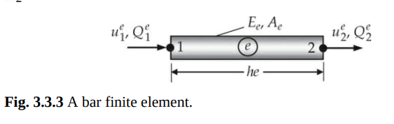
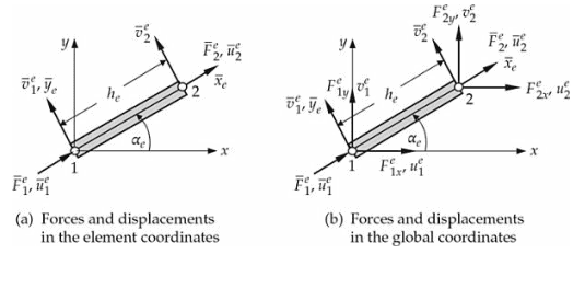
First, we consider a uniform bar element $\Omega^e$ with constant $E_e A_e$ and oriented at an angle $\alpha_e$, measured counterclockwise, from the positive $x$-axis. If the member coordinate system $\left(\bar{x}_e, \bar{y}_e\right)$ is taken as shown in Fig. 6.2.1(a), where denote the displacements and $\left(\bar{F}_i^e, 0\right)$ denote the forces along and transverse to the member at node $i$ with respect to the member coordinate system $\left(\bar{x}_e, \bar{y}_e\right)$, the element equations (3.3.2) can be expressed as:
$$
\frac{E_c A_e}{h_e}\left[\begin{array}{rrrr}
1 & 0 & -1 & 0 \
0 & 0 & 0 & 0 \
-1 & 0 & 1 & 0 \
0 & 0 & 0 & 0
\end{array}\right]\left{\begin{array}{c}
\bar{u}_1^e \
\bar{v}_1^c \
\bar{u}_2^e \
\bar{v}_2^e
\end{array}\right}=\left{\begin{array}{c}
\bar{F}_1^e \
0 \
\bar{F}_2^c \
0
\end{array}\right} \text { or } \overline{\mathbf{K}}^e \bar{\Delta}^e=\overline{\mathbf{F}}^e
$$

数学代写|有限元方法代写Finite Element Method代考|The Truss Element in the Global Coordinates

We wish to write the force-deflection relations in Eq. (6.2.1) in terms of the corresponding global displacements and forces. Toward this end, we first write the transformation relations between the two sets of coordinate systems $(x, y)$ and $\left(\bar{x}_e, \bar{y}_e\right)$ shown in Fig. 6.2.1(a) and (b):
$$
\begin{array}{ll}
\bar{x}_e & =x \cos \alpha_e+y \sin \alpha_e, \quad \bar{y}_e=-x \sin \alpha_e+y \cos \alpha_e \
x=\bar{x}_e \cos \alpha_e-\bar{y}_e \sin \alpha_e, & y=\bar{x}_e \sin \alpha_e+\bar{y}_e \cos \alpha_e
\end{array}
$$
or, in matrix form, we have
$$
\begin{aligned}
&\left{\begin{array}{l}
\bar{x}_e \
\bar{y}_e
\end{array}\right}=\left[\begin{array}{rr}
\cos \alpha_e & \sin \alpha_e \
-\sin \alpha_e & \cos \alpha_e
\end{array}\right]\left{\begin{array}{l}
x \
y
\end{array}\right} \
&\left{\begin{array}{l}
x \
y
\end{array}\right}=\left[\begin{array}{rr}
\cos \alpha_e & -\sin \alpha_e \
\sin \alpha_e & \cos \alpha_e
\end{array}\right]\left{\begin{array}{l}
\bar{x}_e \
\bar{y}_e
\end{array}\right}
\end{aligned}
$$
where $\alpha_e$ is the angle between the positive $x$-axis and positive $\bar{x}_e$-axis, measured in the counterclockwise direction. Note that all quantities with a bar over them are referred to the member (or local) coordinate system $\left(\bar{x}_e, \bar{y}_e\right.$ ), while the quantities without a bar refer to the global coordinates $(x, y)$, as shown in Fig. 6.2.1(b).

The transformation in Eq. (6.2.2) also holds for the components of the displacement and force vectors in the two coordinate systems. To relate $\left(\bar{u}_i, \bar{v}_i\right)$ in the local coordinate system to $\left(u_i, v_i\right)$ in the global coordinate system at both nodes $(i=1,2)$, we write
$$
\left{\begin{array}{c}
\vec{u}_1^e \
\bar{v}_1^e \
\bar{u}_2^e \
\bar{v}_2^e
\end{array}\right}=\left[\begin{array}{cccc}
\cos \alpha_e & \sin \alpha_e & 0 & 0 \
-\sin \alpha_e & \cos \alpha_e & 0 & 0 \
0 & 0 & \cos \alpha_e & \sin \alpha_e \
0 & 0 & -\sin \alpha_e & \cos \alpha_e
\end{array}\right]\left{\begin{array}{c}
u_1^e \
v_1^e \
u_2^e \
v_2^e
\end{array}\right}
$$
or
$$
\bar{\Delta}^e=T^e \Delta^e
$$

where $\bar{\Delta}^e$ and $\Delta^e$ denote the nodal displacement vectors in the member (local) and structure (global) coordinate systems, respectively. Similarly, we have
$$
\overline{\mathbf{F}}^e=\mathbf{T}^e \mathbf{F}^e
$$
where $\overline{\mathbf{F}}^e$ and $\mathbf{F}^e$ are the nodal force vectors in the member and structure coordinate systems, respectively [see Fig. 6.2.1(a) and (b)].

数学代写|有限元方法代写Finite Element Method代考|The Truss Element in the Local Coordinates

有限元方法代考

数学代写|有限元方法代写Finite Element Method代考|The Truss Element in the Local Coordinates

首先,我们考虑一个均匀杆单元$\Omega^e$,其常数为$E_e A_e$,方向为从正$x$ -轴逆时针方向测量的角度$\alpha_e$。取构件坐标系$\left(\bar{x}_e, \bar{y}_e\right)$如图6.2.1(a)所示,其中为相对于构件坐标系$\left(\bar{x}_e, \bar{y}_e\right)$的位移,$\left(\bar{F}_i^e, 0\right)$为节点$i$处的沿力和横向力,则单元方程(3.3.2)可表示为:
$$
\frac{E_c A_e}{h_e}\left[\begin{array}{rrrr}
1 & 0 & -1 & 0 \
0 & 0 & 0 & 0 \
-1 & 0 & 1 & 0 \
0 & 0 & 0 & 0
\end{array}\right]\left{\begin{array}{c}
\bar{u}_1^e \
\bar{v}_1^c \
\bar{u}_2^e \
\bar{v}_2^e
\end{array}\right}=\left{\begin{array}{c}
\bar{F}_1^e \
0 \
\bar{F}_2^c \
0
\end{array}\right} \text { or } \overline{\mathbf{K}}^e \bar{\Delta}^e=\overline{\mathbf{F}}^e
$$

数学代写|有限元方法代写Finite Element Method代考|The Truss Element in the Global Coordinates

我们希望用相应的整体位移和力来表示式(6.2.1)中的力-挠度关系。为此,我们首先写出如图6.2.1(a)和(b)所示的两组坐标系$(x, y)$和$\left(\bar{x}_e, \bar{y}_e\right)$之间的变换关系:
$$
\begin{array}{ll}
\bar{x}_e & =x \cos \alpha_e+y \sin \alpha_e, \quad \bar{y}_e=-x \sin \alpha_e+y \cos \alpha_e \
x=\bar{x}_e \cos \alpha_e-\bar{y}_e \sin \alpha_e, & y=\bar{x}_e \sin \alpha_e+\bar{y}_e \cos \alpha_e
\end{array}
$$
或者,在矩阵形式中,我们有
$$
\begin{aligned}
&\left{\begin{array}{l}
\bar{x}_e \
\bar{y}_e
\end{array}\right}=\left[\begin{array}{rr}
\cos \alpha_e & \sin \alpha_e \
-\sin \alpha_e & \cos \alpha_e
\end{array}\right]\left{\begin{array}{l}
x \
y
\end{array}\right} \
&\left{\begin{array}{l}
x \
y
\end{array}\right}=\left[\begin{array}{rr}
\cos \alpha_e & -\sin \alpha_e \
\sin \alpha_e & \cos \alpha_e
\end{array}\right]\left{\begin{array}{l}
\bar{x}_e \
\bar{y}_e
\end{array}\right}
\end{aligned}
$$
其中$\alpha_e$为正$x$轴与正$\bar{x}_e$轴之间的夹角,以逆时针方向测量。请注意,所有在它们上面有条的量都指向成员(或局部)坐标系$\left(\bar{x}_e, \bar{y}_e\right.$),而没有条的量指向全局坐标$(x, y)$,如图6.2.1(b)所示。

式(6.2.2)中的变换同样适用于两个坐标系中位移矢量和力矢量的分量。要在两个节点$(i=1,2)$上将本地坐标系中的$\left(\bar{u}_i, \bar{v}_i\right)$与全局坐标系中的$\left(u_i, v_i\right)$关联起来,我们这样写
$$
\left{\begin{array}{c}
\vec{u}_1^e \
\bar{v}_1^e \
\bar{u}_2^e \
\bar{v}_2^e
\end{array}\right}=\left[\begin{array}{cccc}
\cos \alpha_e & \sin \alpha_e & 0 & 0 \
-\sin \alpha_e & \cos \alpha_e & 0 & 0 \
0 & 0 & \cos \alpha_e & \sin \alpha_e \
0 & 0 & -\sin \alpha_e & \cos \alpha_e
\end{array}\right]\left{\begin{array}{c}
u_1^e \
v_1^e \
u_2^e \
v_2^e
\end{array}\right}
$$

$$
\bar{\Delta}^e=T^e \Delta^e
$$

其中$\bar{\Delta}^e$和$\Delta^e$分别表示成员(局部)和结构(全局)坐标系中的节点位移向量。类似地,我们有
$$
\overline{\mathbf{F}}^e=\mathbf{T}^e \mathbf{F}^e
$$
其中$\overline{\mathbf{F}}^e$和$\mathbf{F}^e$分别为构件和结构坐标系中的节点力矢量[见图6.2.1(a)和(b)]。

数学代写|有限元方法代写Finite Element Method代考 请认准statistics-lab™

统计代写请认准statistics-lab™. statistics-lab™为您的留学生涯保驾护航。

金融工程代写

金融工程是使用数学技术来解决金融问题。金融工程使用计算机科学、统计学、经济学和应用数学领域的工具和知识来解决当前的金融问题,以及设计新的和创新的金融产品。

非参数统计代写

非参数统计指的是一种统计方法,其中不假设数据来自于由少数参数决定的规定模型;这种模型的例子包括正态分布模型和线性回归模型。

广义线性模型代考

广义线性模型(GLM)归属统计学领域,是一种应用灵活的线性回归模型。该模型允许因变量的偏差分布有除了正态分布之外的其它分布。

术语 广义线性模型(GLM)通常是指给定连续和/或分类预测因素的连续响应变量的常规线性回归模型。它包括多元线性回归,以及方差分析和方差分析(仅含固定效应)。

有限元方法代写

有限元方法(FEM)是一种流行的方法,用于数值解决工程和数学建模中出现的微分方程。典型的问题领域包括结构分析、传热、流体流动、质量运输和电磁势等传统领域。

有限元是一种通用的数值方法,用于解决两个或三个空间变量的偏微分方程(即一些边界值问题)。为了解决一个问题,有限元将一个大系统细分为更小、更简单的部分,称为有限元。这是通过在空间维度上的特定空间离散化来实现的,它是通过构建对象的网格来实现的:用于求解的数值域,它有有限数量的点。边界值问题的有限元方法表述最终导致一个代数方程组。该方法在域上对未知函数进行逼近。[1] 然后将模拟这些有限元的简单方程组合成一个更大的方程系统,以模拟整个问题。然后,有限元通过变化微积分使相关的误差函数最小化来逼近一个解决方案。

tatistics-lab作为专业的留学生服务机构,多年来已为美国、英国、加拿大、澳洲等留学热门地的学生提供专业的学术服务,包括但不限于Essay代写,Assignment代写,Dissertation代写,Report代写,小组作业代写,Proposal代写,Paper代写,Presentation代写,计算机作业代写,论文修改和润色,网课代做,exam代考等等。写作范围涵盖高中,本科,研究生等海外留学全阶段,辐射金融,经济学,会计学,审计学,管理学等全球99%专业科目。写作团队既有专业英语母语作者,也有海外名校硕博留学生,每位写作老师都拥有过硬的语言能力,专业的学科背景和学术写作经验。我们承诺100%原创,100%专业,100%准时,100%满意。

随机分析代写


随机微积分是数学的一个分支,对随机过程进行操作。它允许为随机过程的积分定义一个关于随机过程的一致的积分理论。这个领域是由日本数学家伊藤清在第二次世界大战期间创建并开始的。

时间序列分析代写

随机过程,是依赖于参数的一组随机变量的全体,参数通常是时间。 随机变量是随机现象的数量表现,其时间序列是一组按照时间发生先后顺序进行排列的数据点序列。通常一组时间序列的时间间隔为一恒定值(如1秒,5分钟,12小时,7天,1年),因此时间序列可以作为离散时间数据进行分析处理。研究时间序列数据的意义在于现实中,往往需要研究某个事物其随时间发展变化的规律。这就需要通过研究该事物过去发展的历史记录,以得到其自身发展的规律。

回归分析代写

多元回归分析渐进(Multiple Regression Analysis Asymptotics)属于计量经济学领域,主要是一种数学上的统计分析方法,可以分析复杂情况下各影响因素的数学关系,在自然科学、社会和经济学等多个领域内应用广泛。

MATLAB代写

MATLAB 是一种用于技术计算的高性能语言。它将计算、可视化和编程集成在一个易于使用的环境中,其中问题和解决方案以熟悉的数学符号表示。典型用途包括:数学和计算算法开发建模、仿真和原型制作数据分析、探索和可视化科学和工程图形应用程序开发,包括图形用户界面构建MATLAB 是一个交互式系统,其基本数据元素是一个不需要维度的数组。这使您可以解决许多技术计算问题,尤其是那些具有矩阵和向量公式的问题,而只需用 C 或 Fortran 等标量非交互式语言编写程序所需的时间的一小部分。MATLAB 名称代表矩阵实验室。MATLAB 最初的编写目的是提供对由 LINPACK 和 EISPACK 项目开发的矩阵软件的轻松访问,这两个项目共同代表了矩阵计算软件的最新技术。MATLAB 经过多年的发展,得到了许多用户的投入。在大学环境中,它是数学、工程和科学入门和高级课程的标准教学工具。在工业领域,MATLAB 是高效研究、开发和分析的首选工具。MATLAB 具有一系列称为工具箱的特定于应用程序的解决方案。对于大多数 MATLAB 用户来说非常重要,工具箱允许您学习应用专业技术。工具箱是 MATLAB 函数(M 文件)的综合集合,可扩展 MATLAB 环境以解决特定类别的问题。可用工具箱的领域包括信号处理、控制系统、神经网络、模糊逻辑、小波、仿真等。

R语言代写问卷设计与分析代写
PYTHON代写回归分析与线性模型代写
MATLAB代写方差分析与试验设计代写
STATA代写机器学习/统计学习代写
SPSS代写计量经济学代写
EVIEWS代写时间序列分析代写
EXCEL代写深度学习代写
SQL代写各种数据建模与可视化代写

数学代写|有限元方法代写Finite Element Method代考|Derivation of Element Equations (Finite Element Model)

如果你也在 怎样代写有限元方法finite differences method 这个学科遇到相关的难题,请随时右上角联系我们的24/7代写客服。有限元方法finite differences method在数值分析中,是一类通过用有限差分逼近导数解决微分方程的数值技术。空间域和时间间隔(如果适用)都被离散化,或被分成有限的步骤,通过解决包含有限差分和附近点的数值的代数方程来逼近这些离散点的解的数值。

有限元方法finite differences method有限差分法将可能是非线性的常微分方程(ODE)或偏微分方程(PDE)转换成可以用矩阵代数技术解决的线性方程系统。现代计算机可以有效地进行这些线性代数计算,再加上其相对容易实现,使得FDM在现代数值分析中得到了广泛的应用。今天,FDM与有限元方法一样,是数值解决PDE的最常用方法之一。

statistics-lab™ 为您的留学生涯保驾护航 在代写有限元方法Finite Element Method方面已经树立了自己的口碑, 保证靠谱, 高质且原创的统计Statistics代写服务。我们的专家在代写有限元方法Finite Element Method代写方面经验极为丰富,各种代写有限元方法Finite Element Method相关的作业也就用不着说。

数学代写|有限元方法代写Finite Element Method代考|Derivation of Element Equations (Finite Element Model)

数学代写|有限元方法代写Finite Element Method代考|Derivation of Element Equations (Finite Element Model)

The finite element model (i.e., algebraic equations relating the primary and secondary variables at the element nodes) of the Euler-Bernoulli beam is obtained by substituting the finite element approximation in Eq. (5.2.19) for $w_h^e$ and the $\phi_i^e$ for the weight function $v_i^e$ into the weak form in Eq. (5.2.13). The four different choices $v_1^e=\phi_1^e, v_2^e=\phi_2^e, v_3^e=\phi_3^e$, and $v_4^e=\phi_4^e$ yield a set of four algebraic equations:

$$
\begin{aligned}
0= & \int_{x_e^e}^{x_b^e}\left[E_e I_e \frac{d^2 \phi_1^e}{d x^2}\left(\sum_{j=1}^4 \Delta_j^e \frac{d^2 \phi_j^e}{d x^2}\right)+k_f^e \phi_1^e\left(\sum_{j=1}^4 \Delta_j^e \phi_j^e\right)-\phi_1^e q_e\right] d x \
& -\phi_1^e\left(x_a^e\right) Q_1^e-\left.\left(-\frac{d \phi_1^e}{d x}\right)\right|{x_e^e} Q_2^e-\phi_1^e\left(x_b^e\right) Q_3^e-\left.\left(-\frac{d \phi_1^e}{d x}\right)\right|{x_b^e} Q_4^e \
0= & \int_{x_e^e}^{x_b^e}\left[E_e I_e \frac{d^2 \phi_2^e}{d x^2}\left(\sum_{j=1}^4 \Delta_j^e \frac{d^2 \phi_j^e}{d x^2}\right)+k_f^e \phi_2^e\left(\sum_{j=1}^4 \Delta_j^e \phi_j^e\right)-\phi_2^e q_e\right] d x \
& -\phi_2^e\left(x_a^e\right) Q_1^e-\left.\left(-\frac{d \phi_2^e}{d x}\right)\right|{x_e^e} Q_2^e-\phi_2^e\left(x_b^e\right) Q_3^e-\left.\left(-\frac{d \phi_2^e}{d x}\right)\right|{x_b^e} Q_4^e \
0= & \int_{x_e^e}^{x_b^e}\left[E_e I_e \frac{d^2 \phi_3^e}{d x^2}\left(\sum_{j=1}^4 \Delta_j^e \frac{d^2 \phi_j^e}{d x^2}\right)+k_f^e \phi_3^e\left(\sum_{j=1}^4 \Delta_j^e \phi_j^e\right)-\phi_3^e q_e\right] d x \
& -\phi_3^e\left(x_a^e\right) Q_1^e-\left.\left(-\frac{d \phi_3^e}{d x}\right)\right|{x_e^e} Q_2^e-\phi_3^e\left(x_b^e\right) Q_3^e-\left.\left(-\frac{d \phi_3^e}{d x}\right)\right|{x_b^e} Q_4^e \
0= & \int_{x_e^e}^{x_b^e}\left[E_e I_e \frac{d^2 \phi_4^e}{d x^2}\left(\sum_{j=1}^4 \Delta_j^e \frac{d^2 \phi_j^e}{d x^2}\right)+k_f^e \phi_4^e\left(\sum_{j=1}^4 \Delta_j^e \phi_j^e\right)-\phi_4^e q_e^e\right] d x \
& -\phi_4^e\left(x_a^e\right) Q_1^e-\left.\left(-\frac{d \phi_4^e}{d x}\right)\right|{x_a^e} ^e Q_2^e-\phi_4^e\left(x_b^e\right) Q_3^e-\left.\left(-\frac{d \phi_4^e}{d x}\right)\right|{x_b^e} Q_4^e
\end{aligned}
$$
The ith algebraic equation of the finite element model is given by
$$
0=\sum_{j=1}^4\left[\int_{x_a^e}^{x_b^e}\left(E_e I_e \frac{d^2 \phi_i^e}{d x^2} \frac{d^2 \phi_j^e}{d x^2}+k_f^e \phi_i^e \phi_j^e\right) d x\right] \Delta_j^e-\int_{x_a^e}^{x_b^e} \phi_i^e q_e d x-Q_i^e
$$
or
$$
0=\sum_{j=1}^4 K_{i j}^e \Delta_j^e-q_i^e-Q_i^e=0 \quad \text { or } \quad \mathbf{K}^e \Delta^e=\mathbf{q}^e+\mathbf{Q}^e
$$
where

$$
\begin{aligned}
K_{i j}^e & =\int_{x_e^e}^{x_b^e}\left[E_e(x) I_e(x) \frac{d^2 \phi_i^e}{d x^2} \frac{d^2 \phi_j^e}{d x^2}+k_f^e(x) \phi_i^e \phi_j^e\right] d x \
& =\int_0^{h_e}\left[E_e(\bar{x}) I_e(\bar{x}) \frac{d^2 \phi_i^e}{d \bar{x}^2} \frac{d^2 \phi_j^e}{d \bar{x}^2}+k_f^e(\bar{x}) \phi_i^e \phi_j^e\right] d \bar{x} \
q_i^e & =\int_{x_a^e}^{x_b^e} \phi_i^e(x) q_e(x) d x=\int_0^{h_e} \phi_i^e(\bar{x}) q_e(\bar{x}) d \bar{x}
\end{aligned}
$$
Note that the coefficients $K_{i j}^e$ are symmetric: $K_{i j}^e=K_{j i}^e$ In matrix notation, Eq. (5.2.23) can be written explicitly as
$$
\left[\begin{array}{llll}
K_{11}^e & K_{12}^e & K_{13}^c & K_{14}^e \
K_{21}^e & K_{22}^e & K_{23}^c & K_{24}^e \
K_{31}^e & K_{32}^e & K_{33}^c & K_{34}^e \
K_{41}^c & K_{42}^c & K_{43}^c & K_{44}^e
\end{array}\right]\left{\begin{array}{c}
\Delta_1^e \
\Delta_2^e \
\Delta_3^e \
\Delta_4^e
\end{array}\right}=\left{\begin{array}{l}
q_1^e \
q_2^e \
q_3^e \
q_4^e
\end{array}\right}+\left{\begin{array}{l}
Q_1^e \
Q_2^e \
Q_3^e \
Q_4^e
\end{array}\right}
$$

数学代写|有限元方法代写Finite Element Method代考|Assembly of Element Equations

The assembly procedure for beam elements is the same as that used for bar elements, except that we must take into account the two degrees of freedom at each node. Recall that the assembly of elements is based on (a) interelement continuity of the primary variables (deflection and slope) and (b) inter-element equilibrium of the secondary variable (shear force and bending moment) at the nodes common to elements. To demonstrate the assembly procedure, we select a two-element model shown in Fig. 5.2.9. There are three global nodes and a total of six global generalized displacements and six generalized forces in the problem. The continuity of the primary variables implies the following relation between the element degrees of freedom $\Delta_i^e$ and the global degrees of freedom $U_i$ (see Fig. 5.2.9):

$$
\begin{aligned}
& \Delta_1^1=U_1, \quad \Delta_2^1=U_2, \quad \Delta_3^1=\Delta_1^2=U_3 \
& \Delta_4^1=\Delta_2^2=U_4, \quad \Delta_3^2=U_5, \quad \Delta_4^2=U_6
\end{aligned}
$$
In general, the equilibrium of the generalized forces at a node between two connecting elements $\Omega_e$ and $\Omega_f$ requires that
$$
\begin{aligned}
& Q_3^e+Q_1^f=\text { applied external point force } \
& Q_4^e+Q_2^f=\text { applied external bending moment }
\end{aligned}
$$
If no external applied forces are given, the sum should be equated to zero. In equating the sums to the applied generalized forces (i.e., force or moment), the sign convention for the element force degrees of freedom [see Fig. 5.2.3(c)] should be followed. Forces are taken positive acting in the direction of positive $z$-axis and moments are taken positive when they follow the righthand screw rule (i.e., when thumb is along the positive $y$-axis, the four fingers show the direction of the moment). With respect to the coordinate system used in Figs. 5.2.1 and 5.2.2, forces acting up are positive and clockwise moments are positive.
To impose the equilibrium of forces in Eq. (5.2.30), it is necessary to add the third and fourth equations (corresponding to the second node) of element $\Omega^e$ to the first and second equations (corresponding to the first node) of element $\Omega^f$. Consequently, the global stiffnesses $K_{33}, K_{34}, K_{43}$, and $K_{44}$ associated with global node 2 are the superposition of the element stiffness coefficients:
$$
K_{33}=K_{33}^1+K_{11}^2, K_{34}=K_{34}^1+K_{12}^2, K_{43}=K_{43}^1+K_{21}^2, K_{44}=K_{44}^1+K_{22}^2
$$
In general, the assembled stiffness matrix and force vector for beam elements connected in series have the following forms:
$$
\begin{aligned}
\mathbf{K} & =\left[\begin{array}{cccccc}
K_{11}^1 & K_{12}^1 & K_{13}^1 & K_{14}^1 & 0 & 0 \
K_{21}^1 & K_{22}^1 & K_{23}^1 & K_{24}^1 & 0 & 0 \
K_{31}^1 & K_{32}^1 & K_{33}^1+K_{11}^2 & K_{34}^1+K_{12}^2 & K_{13}^2 & K_{14}^2 \
K_{41}^1 & K_{42}^1 & K_{43}^1+K_{21}^2 & K_{44}^1+K_{22}^2 & K_{23}^2 & K_{24}^2 \
0 & 0 & K_{31}^2 & K_{32}^2 & K_{33}^2 & K_{34}^2 \
0 & 0 & K_{41}^2 & K_{42}^2 & K_{43}^2 & K_{44}^2
\end{array}\right] \
\mathbf{F} & =\left{\begin{array}{c}
q_1^1 \
q_2^1 \
q_3^1+q_1^2 \
q_4^1+q_2^2 \
q_3^2 \
q_4^2
\end{array}\right}+\left{\begin{array}{c}
Q_1^1 \
Q_2^2 \
Q_3^1+Q_1^2 \
Q_4^1+Q_2^2 \
Q_3^2 \
Q_4^2
\end{array}\right}
\end{aligned}
$$

数学代写|有限元方法代写Finite Element Method代考|Derivation of Element Equations (Finite Element Model)

有限元方法代考

数学代写|有限元方法代写Finite Element Method代考|Derivation of Element Equations (Finite Element Model)

将方程(5.2.19)中的有限元近似代入$w_h^e$,将权函数$v_i^e$的$\phi_i^e$代入方程(5.2.13)中的弱形式,得到欧拉-伯努利梁的有限元模型(即单元节点上主次变量的代数方程)。四个不同的选择$v_1^e=\phi_1^e, v_2^e=\phi_2^e, v_3^e=\phi_3^e$,和$v_4^e=\phi_4^e$产生一组四个代数方程:

$$
\begin{aligned}
0= & \int_{x_e^e}^{x_b^e}\left[E_e I_e \frac{d^2 \phi_1^e}{d x^2}\left(\sum_{j=1}^4 \Delta_j^e \frac{d^2 \phi_j^e}{d x^2}\right)+k_f^e \phi_1^e\left(\sum_{j=1}^4 \Delta_j^e \phi_j^e\right)-\phi_1^e q_e\right] d x \
& -\phi_1^e\left(x_a^e\right) Q_1^e-\left.\left(-\frac{d \phi_1^e}{d x}\right)\right|{x_e^e} Q_2^e-\phi_1^e\left(x_b^e\right) Q_3^e-\left.\left(-\frac{d \phi_1^e}{d x}\right)\right|{x_b^e} Q_4^e \
0= & \int_{x_e^e}^{x_b^e}\left[E_e I_e \frac{d^2 \phi_2^e}{d x^2}\left(\sum_{j=1}^4 \Delta_j^e \frac{d^2 \phi_j^e}{d x^2}\right)+k_f^e \phi_2^e\left(\sum_{j=1}^4 \Delta_j^e \phi_j^e\right)-\phi_2^e q_e\right] d x \
& -\phi_2^e\left(x_a^e\right) Q_1^e-\left.\left(-\frac{d \phi_2^e}{d x}\right)\right|{x_e^e} Q_2^e-\phi_2^e\left(x_b^e\right) Q_3^e-\left.\left(-\frac{d \phi_2^e}{d x}\right)\right|{x_b^e} Q_4^e \
0= & \int_{x_e^e}^{x_b^e}\left[E_e I_e \frac{d^2 \phi_3^e}{d x^2}\left(\sum_{j=1}^4 \Delta_j^e \frac{d^2 \phi_j^e}{d x^2}\right)+k_f^e \phi_3^e\left(\sum_{j=1}^4 \Delta_j^e \phi_j^e\right)-\phi_3^e q_e\right] d x \
& -\phi_3^e\left(x_a^e\right) Q_1^e-\left.\left(-\frac{d \phi_3^e}{d x}\right)\right|{x_e^e} Q_2^e-\phi_3^e\left(x_b^e\right) Q_3^e-\left.\left(-\frac{d \phi_3^e}{d x}\right)\right|{x_b^e} Q_4^e \
0= & \int_{x_e^e}^{x_b^e}\left[E_e I_e \frac{d^2 \phi_4^e}{d x^2}\left(\sum_{j=1}^4 \Delta_j^e \frac{d^2 \phi_j^e}{d x^2}\right)+k_f^e \phi_4^e\left(\sum_{j=1}^4 \Delta_j^e \phi_j^e\right)-\phi_4^e q_e^e\right] d x \
& -\phi_4^e\left(x_a^e\right) Q_1^e-\left.\left(-\frac{d \phi_4^e}{d x}\right)\right|{x_a^e} ^e Q_2^e-\phi_4^e\left(x_b^e\right) Q_3^e-\left.\left(-\frac{d \phi_4^e}{d x}\right)\right|{x_b^e} Q_4^e
\end{aligned}
$$
有限元模型的第i代数方程由式给出
$$
0=\sum_{j=1}^4\left[\int_{x_a^e}^{x_b^e}\left(E_e I_e \frac{d^2 \phi_i^e}{d x^2} \frac{d^2 \phi_j^e}{d x^2}+k_f^e \phi_i^e \phi_j^e\right) d x\right] \Delta_j^e-\int_{x_a^e}^{x_b^e} \phi_i^e q_e d x-Q_i^e
$$

$$
0=\sum_{j=1}^4 K_{i j}^e \Delta_j^e-q_i^e-Q_i^e=0 \quad \text { or } \quad \mathbf{K}^e \Delta^e=\mathbf{q}^e+\mathbf{Q}^e
$$
在哪里

$$
\begin{aligned}
K_{i j}^e & =\int_{x_e^e}^{x_b^e}\left[E_e(x) I_e(x) \frac{d^2 \phi_i^e}{d x^2} \frac{d^2 \phi_j^e}{d x^2}+k_f^e(x) \phi_i^e \phi_j^e\right] d x \
& =\int_0^{h_e}\left[E_e(\bar{x}) I_e(\bar{x}) \frac{d^2 \phi_i^e}{d \bar{x}^2} \frac{d^2 \phi_j^e}{d \bar{x}^2}+k_f^e(\bar{x}) \phi_i^e \phi_j^e\right] d \bar{x} \
q_i^e & =\int_{x_a^e}^{x_b^e} \phi_i^e(x) q_e(x) d x=\int_0^{h_e} \phi_i^e(\bar{x}) q_e(\bar{x}) d \bar{x}
\end{aligned}
$$
注意系数$K_{i j}^e$是对称的:$K_{i j}^e=K_{j i}^e$在矩阵表示法中,Eq.(5.2.23)可以显式地写成
$$
\left[\begin{array}{llll}
K_{11}^e & K_{12}^e & K_{13}^c & K_{14}^e \
K_{21}^e & K_{22}^e & K_{23}^c & K_{24}^e \
K_{31}^e & K_{32}^e & K_{33}^c & K_{34}^e \
K_{41}^c & K_{42}^c & K_{43}^c & K_{44}^e
\end{array}\right]\left{\begin{array}{c}
\Delta_1^e \
\Delta_2^e \
\Delta_3^e \
\Delta_4^e
\end{array}\right}=\left{\begin{array}{l}
q_1^e \
q_2^e \
q_3^e \
q_4^e
\end{array}\right}+\left{\begin{array}{l}
Q_1^e \
Q_2^e \
Q_3^e \
Q_4^e
\end{array}\right}
$$

数学代写|有限元方法代写Finite Element Method代考|Assembly of Element Equations

梁单元的装配过程与杆单元的装配过程相同,不同之处在于我们必须考虑每个节点的两个自由度。回想一下,单元的装配是基于(a)主要变量(挠度和坡度)的单元间连续性和(b)次要变量(剪力和弯矩)在单元共同节点上的单元间平衡。为了演示装配过程,我们选择如图5.2.9所示的双元素模型。该问题有3个全局节点,共有6个全局广义位移和6个广义力。主变量的连续性意味着单元自由度$\Delta_i^e$与整体自由度$U_i$之间的关系如下(见图5.2.9):

$$
\begin{aligned}
& \Delta_1^1=U_1, \quad \Delta_2^1=U_2, \quad \Delta_3^1=\Delta_1^2=U_3 \
& \Delta_4^1=\Delta_2^2=U_4, \quad \Delta_3^2=U_5, \quad \Delta_4^2=U_6
\end{aligned}
$$
一般来说,在两个连接单元$\Omega_e$和$\Omega_f$之间的节点上的广义力的平衡要求
$$
\begin{aligned}
& Q_3^e+Q_1^f=\text { applied external point force } \
& Q_4^e+Q_2^f=\text { applied external bending moment }
\end{aligned}
$$
如果没有外力的作用,总和应该等于零。在将总和等同于施加的广义力(即力或力矩)时,应遵循单元力自由度的符号约定[见图5.2.3(c)]。力为正,作用于正$z$ -轴方向,力矩为正,当它们遵循右手螺旋规则时(即,当拇指沿着正$y$ -轴时,四个手指表示力矩方向)。相对于图5.2.1和5.2.2所使用的坐标系,起作用的力为正,顺时针力矩为正。
为了实现式(5.2.30)中的力平衡,需要将单元$\Omega^e$的第三和第四个方程(对应第二个节点)加到单元$\Omega^f$的第一和第二个方程(对应第一个节点)上。因此,与全局节点2相关的全局刚度$K_{33}, K_{34}, K_{43}$和$K_{44}$是单元刚度系数的叠加:
$$
K_{33}=K_{33}^1+K_{11}^2, K_{34}=K_{34}^1+K_{12}^2, K_{43}=K_{43}^1+K_{21}^2, K_{44}=K_{44}^1+K_{22}^2
$$
一般情况下,串联梁单元的组合刚度矩阵和力向量有如下形式:
$$
\begin{aligned}
\mathbf{K} & =\left[\begin{array}{cccccc}
K_{11}^1 & K_{12}^1 & K_{13}^1 & K_{14}^1 & 0 & 0 \
K_{21}^1 & K_{22}^1 & K_{23}^1 & K_{24}^1 & 0 & 0 \
K_{31}^1 & K_{32}^1 & K_{33}^1+K_{11}^2 & K_{34}^1+K_{12}^2 & K_{13}^2 & K_{14}^2 \
K_{41}^1 & K_{42}^1 & K_{43}^1+K_{21}^2 & K_{44}^1+K_{22}^2 & K_{23}^2 & K_{24}^2 \
0 & 0 & K_{31}^2 & K_{32}^2 & K_{33}^2 & K_{34}^2 \
0 & 0 & K_{41}^2 & K_{42}^2 & K_{43}^2 & K_{44}^2
\end{array}\right] \
\mathbf{F} & =\left{\begin{array}{c}
q_1^1 \
q_2^1 \
q_3^1+q_1^2 \
q_4^1+q_2^2 \
q_3^2 \
q_4^2
\end{array}\right}+\left{\begin{array}{c}
Q_1^1 \
Q_2^2 \
Q_3^1+Q_1^2 \
Q_4^1+Q_2^2 \
Q_3^2 \
Q_4^2
\end{array}\right}
\end{aligned}
$$

数学代写|有限元方法代写Finite Element Method代考 请认准statistics-lab™

统计代写请认准statistics-lab™. statistics-lab™为您的留学生涯保驾护航。

金融工程代写

金融工程是使用数学技术来解决金融问题。金融工程使用计算机科学、统计学、经济学和应用数学领域的工具和知识来解决当前的金融问题,以及设计新的和创新的金融产品。

非参数统计代写

非参数统计指的是一种统计方法,其中不假设数据来自于由少数参数决定的规定模型;这种模型的例子包括正态分布模型和线性回归模型。

广义线性模型代考

广义线性模型(GLM)归属统计学领域,是一种应用灵活的线性回归模型。该模型允许因变量的偏差分布有除了正态分布之外的其它分布。

术语 广义线性模型(GLM)通常是指给定连续和/或分类预测因素的连续响应变量的常规线性回归模型。它包括多元线性回归,以及方差分析和方差分析(仅含固定效应)。

有限元方法代写

有限元方法(FEM)是一种流行的方法,用于数值解决工程和数学建模中出现的微分方程。典型的问题领域包括结构分析、传热、流体流动、质量运输和电磁势等传统领域。

有限元是一种通用的数值方法,用于解决两个或三个空间变量的偏微分方程(即一些边界值问题)。为了解决一个问题,有限元将一个大系统细分为更小、更简单的部分,称为有限元。这是通过在空间维度上的特定空间离散化来实现的,它是通过构建对象的网格来实现的:用于求解的数值域,它有有限数量的点。边界值问题的有限元方法表述最终导致一个代数方程组。该方法在域上对未知函数进行逼近。[1] 然后将模拟这些有限元的简单方程组合成一个更大的方程系统,以模拟整个问题。然后,有限元通过变化微积分使相关的误差函数最小化来逼近一个解决方案。

tatistics-lab作为专业的留学生服务机构,多年来已为美国、英国、加拿大、澳洲等留学热门地的学生提供专业的学术服务,包括但不限于Essay代写,Assignment代写,Dissertation代写,Report代写,小组作业代写,Proposal代写,Paper代写,Presentation代写,计算机作业代写,论文修改和润色,网课代做,exam代考等等。写作范围涵盖高中,本科,研究生等海外留学全阶段,辐射金融,经济学,会计学,审计学,管理学等全球99%专业科目。写作团队既有专业英语母语作者,也有海外名校硕博留学生,每位写作老师都拥有过硬的语言能力,专业的学科背景和学术写作经验。我们承诺100%原创,100%专业,100%准时,100%满意。

随机分析代写


随机微积分是数学的一个分支,对随机过程进行操作。它允许为随机过程的积分定义一个关于随机过程的一致的积分理论。这个领域是由日本数学家伊藤清在第二次世界大战期间创建并开始的。

时间序列分析代写

随机过程,是依赖于参数的一组随机变量的全体,参数通常是时间。 随机变量是随机现象的数量表现,其时间序列是一组按照时间发生先后顺序进行排列的数据点序列。通常一组时间序列的时间间隔为一恒定值(如1秒,5分钟,12小时,7天,1年),因此时间序列可以作为离散时间数据进行分析处理。研究时间序列数据的意义在于现实中,往往需要研究某个事物其随时间发展变化的规律。这就需要通过研究该事物过去发展的历史记录,以得到其自身发展的规律。

回归分析代写

多元回归分析渐进(Multiple Regression Analysis Asymptotics)属于计量经济学领域,主要是一种数学上的统计分析方法,可以分析复杂情况下各影响因素的数学关系,在自然科学、社会和经济学等多个领域内应用广泛。

MATLAB代写

MATLAB 是一种用于技术计算的高性能语言。它将计算、可视化和编程集成在一个易于使用的环境中,其中问题和解决方案以熟悉的数学符号表示。典型用途包括:数学和计算算法开发建模、仿真和原型制作数据分析、探索和可视化科学和工程图形应用程序开发,包括图形用户界面构建MATLAB 是一个交互式系统,其基本数据元素是一个不需要维度的数组。这使您可以解决许多技术计算问题,尤其是那些具有矩阵和向量公式的问题,而只需用 C 或 Fortran 等标量非交互式语言编写程序所需的时间的一小部分。MATLAB 名称代表矩阵实验室。MATLAB 最初的编写目的是提供对由 LINPACK 和 EISPACK 项目开发的矩阵软件的轻松访问,这两个项目共同代表了矩阵计算软件的最新技术。MATLAB 经过多年的发展,得到了许多用户的投入。在大学环境中,它是数学、工程和科学入门和高级课程的标准教学工具。在工业领域,MATLAB 是高效研究、开发和分析的首选工具。MATLAB 具有一系列称为工具箱的特定于应用程序的解决方案。对于大多数 MATLAB 用户来说非常重要,工具箱允许您学习应用专业技术。工具箱是 MATLAB 函数(M 文件)的综合集合,可扩展 MATLAB 环境以解决特定类别的问题。可用工具箱的领域包括信号处理、控制系统、神经网络、模糊逻辑、小波、仿真等。

R语言代写问卷设计与分析代写
PYTHON代写回归分析与线性模型代写
MATLAB代写方差分析与试验设计代写
STATA代写机器学习/统计学习代写
SPSS代写计量经济学代写
EVIEWS代写时间序列分析代写
EXCEL代写深度学习代写
SQL代写各种数据建模与可视化代写

数学代写|有限元方法代写Finite Element Method代考|Convergence and Accuracy of Solutions

如果你也在 怎样代写有限元方法finite differences method 这个学科遇到相关的难题,请随时右上角联系我们的24/7代写客服。有限元方法finite differences method在数值分析中,是一类通过用有限差分逼近导数解决微分方程的数值技术。空间域和时间间隔(如果适用)都被离散化,或被分成有限的步骤,通过解决包含有限差分和附近点的数值的代数方程来逼近这些离散点的解的数值。

有限元方法finite differences method有限差分法将可能是非线性的常微分方程(ODE)或偏微分方程(PDE)转换成可以用矩阵代数技术解决的线性方程系统。现代计算机可以有效地进行这些线性代数计算,再加上其相对容易实现,使得FDM在现代数值分析中得到了广泛的应用。今天,FDM与有限元方法一样,是数值解决PDE的最常用方法之一。

statistics-lab™ 为您的留学生涯保驾护航 在代写有限元方法Finite Element Method方面已经树立了自己的口碑, 保证靠谱, 高质且原创的统计Statistics代写服务。我们的专家在代写有限元方法Finite Element Method代写方面经验极为丰富,各种代写有限元方法Finite Element Method相关的作业也就用不着说。

数学代写|有限元方法代写Finite Element Method代考|Convergence and Accuracy of Solutions

数学代写|有限元方法代写Finite Element Method代考|Convergence and Accuracy of Solutions

The finite element solution $u_h$ in Eq. (3.6.1) is said to converge in the energy norm to the true solution $u$ if
$$
\left|u-u_h\right|_m \leq c h^p \text { for } p>0
$$
where $c$ is a constant independent of $u$ and $u_h$ and $h$ is the characteristic length of an element. The constant $p$ is called the rate of convergence. Note that the convergence depends on $h$ as well as on $p$; $p$ depends on the order of the derivative of $u$ in the weak form and the degree of the polynomials used to approximate $u$ [see Eq. (3.6.15)]. Therefore, the error in the approximation can be reduced either by reducing the size of the elements or increasing the degree of approximation. Convergence of the finite element solutions with mesh refinements (i.e., more of the same kind of elements are used) is termed $h$-convergence. Convergence with increasing degree of polynomials is called p-convergence.
Returning to the question of estimating the approximation error, we consider a $2 m$ th-order differential equation in one dimension $(m=1$, secondorder equations; $m=2$, fourth-order equations):
$$
\sum_{i=1}^m(-1)^i \frac{d^i}{d x^i}\left(a_i \frac{d^i u}{d x^i}\right)=f \text { for } 0<x<L
$$
where the coefficients $a_1(x)$ and $a_2(x)$ are assumed to be positive. Suppose that the essential boundary conditions of the problem are
$$
u(0)=u(L)=0 \quad(m=1,2)
$$
when $m=1$ or 2 and
$$
\left.\left(\frac{d u}{d x}\right)\right|{x=0}=\left.\left(\frac{d u}{d x}\right)\right|{x=L}=0
$$
when $m=2$. The variational (or weak) formulation of Eq. (3.6.7) is given by
$$
0=\int_0^L\left(\sum_{i=1}^m a_i \frac{d^i v}{d x^i} \frac{d^i u}{d x^i}-v f\right) d x
$$
The quadratic functional corresponding to the variational form is
$$
I(u)=\int_0^L \frac{1}{2}\left[\sum_{i=1}^m a_i\left(\frac{d^i u}{d x^i}\right)^2\right] d x-\int_0^L u f d x
$$
Now consider a finite element discretization of the domain using $N$ elements of equal length $h$. If $u_h$ denotes the finite element solution in Eq. (3.6.1), we have, from Eq. (3.6.11),
$$
I\left(u_h\right)=\int_0^L \frac{1}{2}\left[\sum_{i=1}^m a_i\left(\frac{d^i u_h}{d x^i}\right)^2\right] d x-\int_0^L u_h f d x
$$

数学代写|有限元方法代写Finite Element Method代考|Governing Equations

The equations governing three-dimensional heat transfer were reviewed in Eqs. (2.6.1)-(2.6.5), and the derivation of one-dimensional heat transfer was presented in Example 1.2.2. The finite element model was developed in Chapter 3 . Here we briefly review the pertinent equations of one-dimensional heat transfer for our use (see [1-4] for additional details). Equations to be reviewed here are one-dimensional analogues of those listed in Eqs. (2.6.2) and (2.6.3), except for the addition of cross-sectional area $A$ of the system.
The Fourier heat conduction law for one-dimensional systems states that the heat flow $q(x)\left(\mathrm{W} / \mathrm{m}^2\right)$ is related to the temperature gradient $\partial T / \partial x$ by (with heat flow in the positive direction of $x$ ),
$$
q=-k \frac{\partial T}{\partial x}
$$
where $k$ is the thermal conductivity of the material $\left[\mathrm{W} /\left(\mathrm{m}^{\circ}{ }^{\circ} \mathrm{C}\right)\right]$ and $T$ the temperature $\left({ }^{\circ} \mathrm{C}\right)$. The negative sign in Eq. (4.2.1) indicates that heat flows downhill (i.e., from high to low) on the temperature scale. The balance of energy requires that
$$
\rho c A \frac{\partial T}{\partial t}-\frac{\partial}{\partial x}\left(k A \frac{\partial T}{\partial x}\right)=A g
$$
where $A$ is the cross-sectional area $\left(\mathrm{m}^2\right), g$ is the internal heat energy generated per unit volume (the unit of $A g$ is $\mathrm{W} / \mathrm{m}), \rho$ is the mass density $\left(\mathrm{kg} / \mathrm{m}^3\right), c$ is the specific heat of the material $\left[\mathrm{J} /\left(\mathrm{kg} \cdot{ }^{\circ} \mathrm{C}\right)\right]$, and $t$ is time (s). Equation (4.2.2) governs the transient heat conduction in a slab or fin (i.e., a one-dimensional system). For plane wall, we take $A=1$.

数学代写|有限元方法代写Finite Element Method代考|Convergence and Accuracy of Solutions

有限元方法代考

数学代写|有限元方法代写Finite Element Method代考|Convergence and Accuracy of Solutions

式(3.6.1)中的有限元解$u_h$在能量范数上收敛于真解$u$ if
$$
\left|u-u_h\right|m \leq c h^p \text { for } p>0 $$ 其中$c$是独立于$u$和$u_h$的常数,$h$是元素的特征长度。常数$p$称为收敛速率。注意,收敛取决于$h$和$p$;$p$取决于$u$弱形式导数的阶数和用于近似$u$的多项式的阶数[见式(3.6.15)]。因此,可以通过减小元素的大小或增加近似程度来减小逼近中的误差。网格细化的有限元解的收敛(即,使用更多的同类元素)被称为$h$ -收敛。多项式随次递增的收敛称为p收敛。 回到估计近似误差的问题,我们考虑一个一维的$2 m$次阶微分方程$(m=1$,二阶方程;$m=2$,四阶方程): $$ \sum{i=1}^m(-1)^i \frac{d^i}{d x^i}\left(a_i \frac{d^i u}{d x^i}\right)=f \text { for } 0<x<L
$$
假设系数$a_1(x)$和$a_2(x)$为正。设问题的基本边界条件为
$$
u(0)=u(L)=0 \quad(m=1,2)
$$
当$m=1$或2和
$$
\left.\left(\frac{d u}{d x}\right)\right|{x=0}=\left.\left(\frac{d u}{d x}\right)\right|{x=L}=0
$$
当$m=2$。式(3.6.7)的变分(或弱)形式由式给出
$$
0=\int_0^L\left(\sum_{i=1}^m a_i \frac{d^i v}{d x^i} \frac{d^i u}{d x^i}-v f\right) d x
$$
变分形式对应的二次泛函为
$$
I(u)=\int_0^L \frac{1}{2}\left[\sum_{i=1}^m a_i\left(\frac{d^i u}{d x^i}\right)^2\right] d x-\int_0^L u f d x
$$
现在考虑使用$N$等长$h$单元的域的有限元离散化。设$u_h$为式(3.6.1)中的有限元解,由式(3.6.11)可得:
$$
I\left(u_h\right)=\int_0^L \frac{1}{2}\left[\sum_{i=1}^m a_i\left(\frac{d^i u_h}{d x^i}\right)^2\right] d x-\int_0^L u_h f d x
$$

数学代写|有限元方法代写Finite Element Method代考|Governing Equations

对三维传热方程进行了综述。(2.6.1)-(2.6.5),一维传热的推导见例1.2.2。第三章建立了有限元模型。在这里,我们简要回顾一下一维传热的相关方程,以供我们使用(详见[1-4])。这里要回顾的方程是方程中列出的一维类似物。(2.6.2)和(2.6.3),但系统截面积$A$的增加除外。
一维系统的傅里叶热传导定律表明,热流$q(x)\left(\mathrm{W} / \mathrm{m}^2\right)$与温度梯度$\partial T / \partial x$的关系为(热流正向$x$),
$$
q=-k \frac{\partial T}{\partial x}
$$
其中$k$为材料的导热系数$\left[\mathrm{W} /\left(\mathrm{m}^{\circ}{ }^{\circ} \mathrm{C}\right)\right]$, $T$为温度$\left({ }^{\circ} \mathrm{C}\right)$。式(4.2.1)中的负号表示热量在温标上向下流动(即从高到低)。能量平衡需要这样
$$
\rho c A \frac{\partial T}{\partial t}-\frac{\partial}{\partial x}\left(k A \frac{\partial T}{\partial x}\right)=A g
$$
式中$A$为截面积$\left(\mathrm{m}^2\right), g$为单位体积内产生的内部热能($A g$的单位为$\mathrm{W} / \mathrm{m}), \rho$为质量密度$\left(\mathrm{kg} / \mathrm{m}^3\right), c$为材料的比热$\left[\mathrm{J} /\left(\mathrm{kg} \cdot{ }^{\circ} \mathrm{C}\right)\right]$, $t$为时间(s)。式(4.2.2)支配板或翅片(即一维系统)的瞬态热传导。对于平面墙,我们取$A=1$。

数学代写|有限元方法代写Finite Element Method代考 请认准statistics-lab™

统计代写请认准statistics-lab™. statistics-lab™为您的留学生涯保驾护航。

金融工程代写

金融工程是使用数学技术来解决金融问题。金融工程使用计算机科学、统计学、经济学和应用数学领域的工具和知识来解决当前的金融问题,以及设计新的和创新的金融产品。

非参数统计代写

非参数统计指的是一种统计方法,其中不假设数据来自于由少数参数决定的规定模型;这种模型的例子包括正态分布模型和线性回归模型。

广义线性模型代考

广义线性模型(GLM)归属统计学领域,是一种应用灵活的线性回归模型。该模型允许因变量的偏差分布有除了正态分布之外的其它分布。

术语 广义线性模型(GLM)通常是指给定连续和/或分类预测因素的连续响应变量的常规线性回归模型。它包括多元线性回归,以及方差分析和方差分析(仅含固定效应)。

有限元方法代写

有限元方法(FEM)是一种流行的方法,用于数值解决工程和数学建模中出现的微分方程。典型的问题领域包括结构分析、传热、流体流动、质量运输和电磁势等传统领域。

有限元是一种通用的数值方法,用于解决两个或三个空间变量的偏微分方程(即一些边界值问题)。为了解决一个问题,有限元将一个大系统细分为更小、更简单的部分,称为有限元。这是通过在空间维度上的特定空间离散化来实现的,它是通过构建对象的网格来实现的:用于求解的数值域,它有有限数量的点。边界值问题的有限元方法表述最终导致一个代数方程组。该方法在域上对未知函数进行逼近。[1] 然后将模拟这些有限元的简单方程组合成一个更大的方程系统,以模拟整个问题。然后,有限元通过变化微积分使相关的误差函数最小化来逼近一个解决方案。

tatistics-lab作为专业的留学生服务机构,多年来已为美国、英国、加拿大、澳洲等留学热门地的学生提供专业的学术服务,包括但不限于Essay代写,Assignment代写,Dissertation代写,Report代写,小组作业代写,Proposal代写,Paper代写,Presentation代写,计算机作业代写,论文修改和润色,网课代做,exam代考等等。写作范围涵盖高中,本科,研究生等海外留学全阶段,辐射金融,经济学,会计学,审计学,管理学等全球99%专业科目。写作团队既有专业英语母语作者,也有海外名校硕博留学生,每位写作老师都拥有过硬的语言能力,专业的学科背景和学术写作经验。我们承诺100%原创,100%专业,100%准时,100%满意。

随机分析代写


随机微积分是数学的一个分支,对随机过程进行操作。它允许为随机过程的积分定义一个关于随机过程的一致的积分理论。这个领域是由日本数学家伊藤清在第二次世界大战期间创建并开始的。

时间序列分析代写

随机过程,是依赖于参数的一组随机变量的全体,参数通常是时间。 随机变量是随机现象的数量表现,其时间序列是一组按照时间发生先后顺序进行排列的数据点序列。通常一组时间序列的时间间隔为一恒定值(如1秒,5分钟,12小时,7天,1年),因此时间序列可以作为离散时间数据进行分析处理。研究时间序列数据的意义在于现实中,往往需要研究某个事物其随时间发展变化的规律。这就需要通过研究该事物过去发展的历史记录,以得到其自身发展的规律。

回归分析代写

多元回归分析渐进(Multiple Regression Analysis Asymptotics)属于计量经济学领域,主要是一种数学上的统计分析方法,可以分析复杂情况下各影响因素的数学关系,在自然科学、社会和经济学等多个领域内应用广泛。

MATLAB代写

MATLAB 是一种用于技术计算的高性能语言。它将计算、可视化和编程集成在一个易于使用的环境中,其中问题和解决方案以熟悉的数学符号表示。典型用途包括:数学和计算算法开发建模、仿真和原型制作数据分析、探索和可视化科学和工程图形应用程序开发,包括图形用户界面构建MATLAB 是一个交互式系统,其基本数据元素是一个不需要维度的数组。这使您可以解决许多技术计算问题,尤其是那些具有矩阵和向量公式的问题,而只需用 C 或 Fortran 等标量非交互式语言编写程序所需的时间的一小部分。MATLAB 名称代表矩阵实验室。MATLAB 最初的编写目的是提供对由 LINPACK 和 EISPACK 项目开发的矩阵软件的轻松访问,这两个项目共同代表了矩阵计算软件的最新技术。MATLAB 经过多年的发展,得到了许多用户的投入。在大学环境中,它是数学、工程和科学入门和高级课程的标准教学工具。在工业领域,MATLAB 是高效研究、开发和分析的首选工具。MATLAB 具有一系列称为工具箱的特定于应用程序的解决方案。对于大多数 MATLAB 用户来说非常重要,工具箱允许您学习应用专业技术。工具箱是 MATLAB 函数(M 文件)的综合集合,可扩展 MATLAB 环境以解决特定类别的问题。可用工具箱的领域包括信号处理、控制系统、神经网络、模糊逻辑、小波、仿真等。

R语言代写问卷设计与分析代写
PYTHON代写回归分析与线性模型代写
MATLAB代写方差分析与试验设计代写
STATA代写机器学习/统计学习代写
SPSS代写计量经济学代写
EVIEWS代写时间序列分析代写
EXCEL代写深度学习代写
SQL代写各种数据建模与可视化代写

数学代写|有限元方法代写Finite Element Method代考|Model Equation

如果你也在 怎样代写有限元方法finite differences method 这个学科遇到相关的难题,请随时右上角联系我们的24/7代写客服。有限元方法finite differences method在数值分析中,是一类通过用有限差分逼近导数解决微分方程的数值技术。空间域和时间间隔(如果适用)都被离散化,或被分成有限的步骤,通过解决包含有限差分和附近点的数值的代数方程来逼近这些离散点的解的数值。

有限元方法finite differences method有限差分法将可能是非线性的常微分方程(ODE)或偏微分方程(PDE)转换成可以用矩阵代数技术解决的线性方程系统。现代计算机可以有效地进行这些线性代数计算,再加上其相对容易实现,使得FDM在现代数值分析中得到了广泛的应用。今天,FDM与有限元方法一样,是数值解决PDE的最常用方法之一。

statistics-lab™ 为您的留学生涯保驾护航 在代写有限元方法Finite Element Method方面已经树立了自己的口碑, 保证靠谱, 高质且原创的统计Statistics代写服务。我们的专家在代写有限元方法Finite Element Method代写方面经验极为丰富,各种代写有限元方法Finite Element Method相关的作业也就用不着说。

数学代写|有限元方法代写Finite Element Method代考|Model Equation

数学代写|有限元方法代写Finite Element Method代考|Model Equation

Consider the second-order differential equation in vector form
$$
-\nabla \cdot(\mathbf{a} \cdot \nabla u)=f(\mathbf{x})
$$

where $\nabla$ is the gradient operator discussed in Section 2.2.1.3, a is a known second-order tensor, $u$ is the field variable to be determined, and $f$ is a known source. An example of Eq. (3.5.1) is provided by heat conduction equation (see Reddy $[1,4])$ where $u$ is the temperature, $\mathbf{a}$ is the conductivity tensor, and $f$ is the internal heat generation.

The equations governing physical processes in cylindrical geometries are described analytically in terms of cylindrical coordinates $(r, \theta, z)$. For isotropic material (i.e., $a_{r r}=a_{\theta \theta}=a_{z z} \equiv a$ ), Eq. (3.5.1) takes the form
$$
-\frac{1}{r} \frac{\partial}{\partial r}\left(r a \frac{\partial u}{\partial r}\right)-\frac{1}{r} \frac{\partial}{\partial \theta}\left(\frac{a}{r} \frac{\partial u}{\partial \theta}\right)-\frac{\partial}{\partial z}\left(a \frac{\partial u}{\partial z}\right)=f(r, \theta, z)
$$
When the geometry, loading, and boundary conditions are independent of the circumferential direction (i.e., $\theta$-coordinate direction), the problem is said to be axisymmetric and the governing equations become two-dimensional in terms of $r$ and $z$. In addition, if the problem geometry and data are independent of $z$, for example, when the cylinder is very long, the equations are functions of only the radial coordinate $r$, as shown in Fig. 1.4.6, which is reproduced in Fig. 3.5.1(a) through (c):
$$
-\frac{1}{r} \frac{d}{d r}\left[r a(r) \frac{d u}{d r}\right]=f(r) \text { for } \quad R_i<r<R_0
$$
where $r$ is the radial coordinate, $a$ and $f$ are known functions of $r$, and $u$ is the dependent variable. Such equations arise, for example, in connection with radial heat flow in a long circular cylinder of inner radius $R_i \geq 0$ and outer radius $R_0$. The radially symmetric conditions require that both $a=k$ ( $k$ is the conductivity) and $f$ (internal heat generation) be functions of only $r$. In this section we develop the finite element model of one-dimensional axisymmetric problems described by Eq. (3.5.3).

数学代写|有限元方法代写Finite Element Method代考|Weak Form

We begin with the development of the weak form, where the volume element in the weighted-integral statement is replaced by $d v=r d r d \theta d z$. Since the integrand is independent of both $\theta$ and $z$ and considering cylinder of unit length, we obtain
$$
\int_{\sigma^f} F(r) d v=\int_0^1 \int_0^{2 \pi} \int_{r_a}^{r_b} F(r) r d r d \theta d z=2 \pi \int_{r_a}^{r_b} F(r) r d r
$$
where $\left(r_a, r_b\right)$ is the domain of a typical element along the radial direction. Next, we carry out the remaining two steps of the weak formulation.
In developing the weak form of Eq. (3.5.3), we replace $u$ with its approximation $u_h^e$ multiply resulting residual with a weight function $w_i^e(r)$, and integrate over the element volume of the cylinder of unit length (see Fig. 3.5.1):
$$
\begin{aligned}
& 0=2 \pi \int_{r_a}^{r_b} w_i^e\left[-\frac{1}{r} \frac{d}{d r}\left(r a \frac{d u_h}{d r}\right)-f\right] r d r \
& 0=2 \pi \int_{r_a}^{r_b}\left(a \frac{d w_i}{d r} \frac{d u_h}{d r}-w_i f\right) r d r-2 \pi\left[w_i^e r a \frac{d u_h}{d r}\right]_{r_a}^{r_b}
\end{aligned}
$$

\begin{aligned}
& 0=2 \pi \int_{r_a}^{r_b}\left(a \frac{d w_i}{d r} \frac{d u_h}{d r}-w_i f\right) r d r-w_i^e\left(r_a\right) Q_1^e-w_i^e\left(r_b\right) Q_2^e \
& Q_1^e \equiv-\left.2 \pi\left(r a \frac{d u_h}{d r}\right)\right|{r_a},\left.\quad Q_2^e \equiv 2 \pi\left(r a \frac{d u_h}{d r}\right)\right|{r_b}
\end{aligned}

数学代写|有限元方法代写Finite Element Method代考|Model Equation

有限元方法代考

数学代写|有限元方法代写Finite Element Method代考|Model Equation

考虑矢量形式的二阶微分方程
$$
-\nabla \cdot(\mathbf{a} \cdot \nabla u)=f(\mathbf{x})
$$

其中$\nabla$为2.2.1.3节讨论的梯度算子,a为已知二阶张量,$u$为待确定的场变量,$f$为已知源。(3.5.1)式的一个例子是热传导方程(参见Reddy $[1,4])$),其中$u$为温度,$\mathbf{a}$为传导张量,$f$为内部产热。

控制圆柱形几何中物理过程的方程用柱坐标$(r, \theta, z)$进行了解析描述。对于各向同性材料(即$a_{r r}=a_{\theta \theta}=a_{z z} \equiv a$),式(3.5.1)的形式为
$$
-\frac{1}{r} \frac{\partial}{\partial r}\left(r a \frac{\partial u}{\partial r}\right)-\frac{1}{r} \frac{\partial}{\partial \theta}\left(\frac{a}{r} \frac{\partial u}{\partial \theta}\right)-\frac{\partial}{\partial z}\left(a \frac{\partial u}{\partial z}\right)=f(r, \theta, z)
$$
当几何、载荷和边界条件与周向(即$\theta$ -坐标方向)无关时,问题被认为是轴对称的,控制方程变为$r$和$z$的二维形式。此外,如果问题几何和数据与$z$无关,例如当圆柱体很长时,则方程仅为径向坐标$r$的函数,如图1.4.6所示,如图3.5.1(a)至(c)所示:
$$
-\frac{1}{r} \frac{d}{d r}\left[r a(r) \frac{d u}{d r}\right]=f(r) \text { for } \quad R_i<r<R_0
$$
其中$r$为径向坐标,$a$和$f$为$r$的已知函数,$u$为因变量。例如,这样的方程出现在与内半径$R_i \geq 0$和外半径$R_0$的长圆柱体的径向热流有关的情况下。径向对称条件要求$a=k$ ($k$是电导率)和$f$(内部产热)仅是$r$的函数。在本节中,我们建立了由式(3.5.3)描述的一维轴对称问题的有限元模型。

数学代写|有限元方法代写Finite Element Method代考|Weak Form

我们从弱形式的发展开始,其中加权积分语句中的体积元被$d v=r d r d \theta d z$取代。由于被积函数与$\theta$和$z$无关,且考虑单位长度的圆柱体,我们得到
$$
\int_{\sigma^f} F(r) d v=\int_0^1 \int_0^{2 \pi} \int_{r_a}^{r_b} F(r) r d r d \theta d z=2 \pi \int_{r_a}^{r_b} F(r) r d r
$$
式中$\left(r_a, r_b\right)$为典型单元沿径向的域。接下来,我们进行弱公式的剩余两步。
在开发弱形式的Eq.(3.5.3)时,我们将$u$替换为其近似值$u_h^e$,将所得残差与权函数$w_i^e(r)$相乘,并对单位长度圆柱体的单元体积进行积分(见图3.5.1):
$$
\begin{aligned}
& 0=2 \pi \int_{r_a}^{r_b} w_i^e\left[-\frac{1}{r} \frac{d}{d r}\left(r a \frac{d u_h}{d r}\right)-f\right] r d r \
& 0=2 \pi \int_{r_a}^{r_b}\left(a \frac{d w_i}{d r} \frac{d u_h}{d r}-w_i f\right) r d r-2 \pi\left[w_i^e r a \frac{d u_h}{d r}\right]_{r_a}^{r_b}
\end{aligned}
$$

\begin{aligned}
& 0=2 \pi \int_{r_a}^{r_b}\left(a) \frac{d w_i}{d r} \frac{d u_h}{d r}-w_i f\right) r d r-w_i^e\left[au:]\right) Q_1^e-w_i^e\left(b)\right) Q_2^e \& Q_1^e \equiv-\left.2 \pi\left(r a) \frac{d u_h}{d r}\right)\right|{r_a},\left.\quad Q_2^e \equiv 2 \pi\left(r a) \frac{d u_h}{d r}\right)\right|{r_b}
\end{aligned}

数学代写|有限元方法代写Finite Element Method代考 请认准statistics-lab™

统计代写请认准statistics-lab™. statistics-lab™为您的留学生涯保驾护航。

金融工程代写

金融工程是使用数学技术来解决金融问题。金融工程使用计算机科学、统计学、经济学和应用数学领域的工具和知识来解决当前的金融问题,以及设计新的和创新的金融产品。

非参数统计代写

非参数统计指的是一种统计方法,其中不假设数据来自于由少数参数决定的规定模型;这种模型的例子包括正态分布模型和线性回归模型。

广义线性模型代考

广义线性模型(GLM)归属统计学领域,是一种应用灵活的线性回归模型。该模型允许因变量的偏差分布有除了正态分布之外的其它分布。

术语 广义线性模型(GLM)通常是指给定连续和/或分类预测因素的连续响应变量的常规线性回归模型。它包括多元线性回归,以及方差分析和方差分析(仅含固定效应)。

有限元方法代写

有限元方法(FEM)是一种流行的方法,用于数值解决工程和数学建模中出现的微分方程。典型的问题领域包括结构分析、传热、流体流动、质量运输和电磁势等传统领域。

有限元是一种通用的数值方法,用于解决两个或三个空间变量的偏微分方程(即一些边界值问题)。为了解决一个问题,有限元将一个大系统细分为更小、更简单的部分,称为有限元。这是通过在空间维度上的特定空间离散化来实现的,它是通过构建对象的网格来实现的:用于求解的数值域,它有有限数量的点。边界值问题的有限元方法表述最终导致一个代数方程组。该方法在域上对未知函数进行逼近。[1] 然后将模拟这些有限元的简单方程组合成一个更大的方程系统,以模拟整个问题。然后,有限元通过变化微积分使相关的误差函数最小化来逼近一个解决方案。

tatistics-lab作为专业的留学生服务机构,多年来已为美国、英国、加拿大、澳洲等留学热门地的学生提供专业的学术服务,包括但不限于Essay代写,Assignment代写,Dissertation代写,Report代写,小组作业代写,Proposal代写,Paper代写,Presentation代写,计算机作业代写,论文修改和润色,网课代做,exam代考等等。写作范围涵盖高中,本科,研究生等海外留学全阶段,辐射金融,经济学,会计学,审计学,管理学等全球99%专业科目。写作团队既有专业英语母语作者,也有海外名校硕博留学生,每位写作老师都拥有过硬的语言能力,专业的学科背景和学术写作经验。我们承诺100%原创,100%专业,100%准时,100%满意。

随机分析代写


随机微积分是数学的一个分支,对随机过程进行操作。它允许为随机过程的积分定义一个关于随机过程的一致的积分理论。这个领域是由日本数学家伊藤清在第二次世界大战期间创建并开始的。

时间序列分析代写

随机过程,是依赖于参数的一组随机变量的全体,参数通常是时间。 随机变量是随机现象的数量表现,其时间序列是一组按照时间发生先后顺序进行排列的数据点序列。通常一组时间序列的时间间隔为一恒定值(如1秒,5分钟,12小时,7天,1年),因此时间序列可以作为离散时间数据进行分析处理。研究时间序列数据的意义在于现实中,往往需要研究某个事物其随时间发展变化的规律。这就需要通过研究该事物过去发展的历史记录,以得到其自身发展的规律。

回归分析代写

多元回归分析渐进(Multiple Regression Analysis Asymptotics)属于计量经济学领域,主要是一种数学上的统计分析方法,可以分析复杂情况下各影响因素的数学关系,在自然科学、社会和经济学等多个领域内应用广泛。

MATLAB代写

MATLAB 是一种用于技术计算的高性能语言。它将计算、可视化和编程集成在一个易于使用的环境中,其中问题和解决方案以熟悉的数学符号表示。典型用途包括:数学和计算算法开发建模、仿真和原型制作数据分析、探索和可视化科学和工程图形应用程序开发,包括图形用户界面构建MATLAB 是一个交互式系统,其基本数据元素是一个不需要维度的数组。这使您可以解决许多技术计算问题,尤其是那些具有矩阵和向量公式的问题,而只需用 C 或 Fortran 等标量非交互式语言编写程序所需的时间的一小部分。MATLAB 名称代表矩阵实验室。MATLAB 最初的编写目的是提供对由 LINPACK 和 EISPACK 项目开发的矩阵软件的轻松访问,这两个项目共同代表了矩阵计算软件的最新技术。MATLAB 经过多年的发展,得到了许多用户的投入。在大学环境中,它是数学、工程和科学入门和高级课程的标准教学工具。在工业领域,MATLAB 是高效研究、开发和分析的首选工具。MATLAB 具有一系列称为工具箱的特定于应用程序的解决方案。对于大多数 MATLAB 用户来说非常重要,工具箱允许您学习应用专业技术。工具箱是 MATLAB 函数(M 文件)的综合集合,可扩展 MATLAB 环境以解决特定类别的问题。可用工具箱的领域包括信号处理、控制系统、神经网络、模糊逻辑、小波、仿真等。

R语言代写问卷设计与分析代写
PYTHON代写回归分析与线性模型代写
MATLAB代写方差分析与试验设计代写
STATA代写机器学习/统计学习代写
SPSS代写计量经济学代写
EVIEWS代写时间序列分析代写
EXCEL代写深度学习代写
SQL代写各种数据建模与可视化代写

数学代写|有限元方法代写Finite Element Method代考|Axial Deformation of Elastic Bars

如果你也在 怎样代写有限元方法finite differences method 这个学科遇到相关的难题,请随时右上角联系我们的24/7代写客服。有限元方法finite differences method在数值分析中,是一类通过用有限差分逼近导数解决微分方程的数值技术。空间域和时间间隔(如果适用)都被离散化,或被分成有限的步骤,通过解决包含有限差分和附近点的数值的代数方程来逼近这些离散点的解的数值。

有限元方法finite differences method有限差分法将可能是非线性的常微分方程(ODE)或偏微分方程(PDE)转换成可以用矩阵代数技术解决的线性方程系统。现代计算机可以有效地进行这些线性代数计算,再加上其相对容易实现,使得FDM在现代数值分析中得到了广泛的应用。今天,FDM与有限元方法一样,是数值解决PDE的最常用方法之一。

statistics-lab™ 为您的留学生涯保驾护航 在代写有限元方法Finite Element Method方面已经树立了自己的口碑, 保证靠谱, 高质且原创的统计Statistics代写服务。我们的专家在代写有限元方法Finite Element Method代写方面经验极为丰富,各种代写有限元方法Finite Element Method相关的作业也就用不着说。

数学代写|有限元方法代写Finite Element Method代考|Axial Deformation of Elastic Bars

数学代写|有限元方法代写Finite Element Method代考|Axial Deformation of Elastic Bars

For small axial deformations of a homogeneous and isotropic bar with uniform cross section, the element equations are obtained directly from the definitions of stress and strain and the stress-strain relation. For example, consider the free-body diagram of a bar element of length $h_e$, areas of cross section $A_e$, and modulus of elasticity $E_e$, and subjected to end forces $Q_1^e$ and $Q_{\text {, }}^e$, as shown in Fig. 3.3.3.
From a course on mechanics of deformable solids, we have
strain, $\varepsilon^e=$ elongation/original length $=\delta_e / h_e$
stress, $\sigma^e=$ modulus of elasticity $\times \operatorname{strain}=E_e \varepsilon^e$
load, $Q^e=$ stress $\times$ area of cross section $=\sigma^e A_e$
The strain defined above is the average (or engineering) strain.
Mathematically, strain for one-dimensional problems is defined as $\varepsilon=d u / d x$, $u$ being displacement, which includes rigid body motion as well as elongation of the bar. The (compressive) force at the left end of the bar element is
$$
Q_1^e=A_e \sigma_1^e=A_e E_e \varepsilon_1^e=A_e E_e \frac{u_1^e-u_2^e}{h_e}=\frac{A_e E_e}{h_e}\left(u_1^e-u_2^e\right)
$$
where $E_e$ is the Young’s modulus of the bar element. Similarly, the force at the right end is
$$
Q_2^e=\frac{A_e E_e}{h_e}\left(u_2^e-u_1^e\right)
$$
In matrix form, these relations can be expressed as
$$
k_e\left[\begin{array}{rr}
1 & -1 \
-1 & 1
\end{array}\right]\left{\begin{array}{l}
u_1^e \
u_2^e
\end{array}\right}=\left{\begin{array}{l}
Q_1^e \
Q_2^e
\end{array}\right}, k_e=\frac{A_e E_e}{h_e}\left(\text { or } \mathbf{K}^e \mathbf{u}^e=\mathbf{Q}^e\right. \text { ) }
$$

数学代写|有限元方法代写Finite Element Method代考|Torsion of Circular Shafts

Another problem that can be directly formulated as a discrete element is the torsion of a circular shaft shown in Fig. 3.3.5(a). From a course on mechanics of deformable solids, the angle of twist $\theta$ of an elastic, constant cross section, circular cylindrical member is related to torque $T$ (about the longitudinal axis of the member) by
$$
T=\frac{G J}{L} \theta \equiv k \theta, k=\frac{G J}{L}
$$

where $J$ is the polar moment of area, $L$ is the length, and $G$ is the shear modulus of the material of the shaft. The above equation can be used to write a relationship between the end torques $\left(T_1^e, T_2^e\right)$ and the end twists $\left(\theta_1^e, \theta_2^e\right)$ of a circular cylindrical member of length $h_e$, as shown in Fig. 3.3.5(b):
$$
T_1^e=k_e\left(\theta_1^e-\theta_2^e\right), T_2^e=k_e\left(\theta_2^e-\theta_1^e\right), k_e=\frac{G_e J_e}{h_\alpha}
$$
or, in matrix form,
$$
k_e\left[\begin{array}{rr}
1 & -1 \
-1 & 1
\end{array}\right]\left{\begin{array}{l}
\theta_1^e \
\theta_2^e
\end{array}\right}=\left{\begin{array}{l}
T_1^e \
T_2^e
\end{array}\right}
$$
Once again, we have the same finite element equations with different symbols and for different physics. We can interpret that the torsional spring constant is equal to $k_e=G_e J_e / h_e$. The nice part of using Eq. (3.3.24) is that it includes both kinematics and force balance. Consequently, solving indeterminate problems is very easy compared to the strength of materials approach.

数学代写|有限元方法代写Finite Element Method代考|Axial Deformation of Elastic Bars

有限元方法代考

数学代写|有限元方法代写Finite Element Method代考|Axial Deformation of Elastic Bars

对于等截面均质各向同性杆的小轴向变形,可直接从应力应变和应力-应变关系的定义中得到单元方程。例如,考虑长度为$h_e$、截面面积为$A_e$、弹性模量为$E_e$的杆元在端力$Q_1^e$和$Q_{\text {, }}^e$作用下的自由体图,如图3.3.3所示。
在可变形固体力学的课程中,我们有
应变,$\varepsilon^e=$伸长率/原始长度$=\delta_e / h_e$
应力,$\sigma^e=$弹性模量$\times \operatorname{strain}=E_e \varepsilon^e$
荷载,$Q^e=$应力$\times$截面面积$=\sigma^e A_e$
以上定义的应变是平均(或工程)应变。
数学上,一维问题的应变定义为$\varepsilon=d u / d x$, $u$为位移,其中包括刚体运动和杆的伸长。杆单元左端(压缩)力为
$$
Q_1^e=A_e \sigma_1^e=A_e E_e \varepsilon_1^e=A_e E_e \frac{u_1^e-u_2^e}{h_e}=\frac{A_e E_e}{h_e}\left(u_1^e-u_2^e\right)
$$
其中$E_e$为杆单元的杨氏模量。同样,右端的力为
$$
Q_2^e=\frac{A_e E_e}{h_e}\left(u_2^e-u_1^e\right)
$$
在矩阵形式中,这些关系可以表示为
$$
k_e\left[\begin{array}{rr}
1 & -1 \
-1 & 1
\end{array}\right]\left{\begin{array}{l}
u_1^e \
u_2^e
\end{array}\right}=\left{\begin{array}{l}
Q_1^e \
Q_2^e
\end{array}\right}, k_e=\frac{A_e E_e}{h_e}\left(\text { or } \mathbf{K}^e \mathbf{u}^e=\mathbf{Q}^e\right. \text { ) }
$$

数学代写|有限元方法代写Finite Element Method代考|Torsion of Circular Shafts

另一个可以直接表述为离散单元的问题是如图3.3.5(a)所示的圆轴的扭转。在可变形固体力学课程中,一个弹性的、恒定截面的圆筒形构件的扭转角$\theta$与扭矩$T$(关于构件的纵轴)的关系为
$$
T=\frac{G J}{L} \theta \equiv k \theta, k=\frac{G J}{L}
$$

式中$J$为面积极矩,$L$为长度,$G$为轴材料的剪切模量。由上式可以写出长度为$h_e$的圆柱构件的端力矩$\left(T_1^e, T_2^e\right)$与端扭$\left(\theta_1^e, \theta_2^e\right)$的关系,如图3.3.5(b)所示:
$$
T_1^e=k_e\left(\theta_1^e-\theta_2^e\right), T_2^e=k_e\left(\theta_2^e-\theta_1^e\right), k_e=\frac{G_e J_e}{h_\alpha}
$$
或者,用矩阵的形式,
$$
k_e\left[\begin{array}{rr}
1 & -1 \
-1 & 1
\end{array}\right]\left{\begin{array}{l}
\theta_1^e \
\theta_2^e
\end{array}\right}=\left{\begin{array}{l}
T_1^e \
T_2^e
\end{array}\right}
$$
同样,我们有相同的有限元方程,不同的符号,不同的物理。我们可以解释为扭转弹簧常数等于$k_e=G_e J_e / h_e$。使用Eq.(3.3.24)的好处是它包括运动学和力平衡。因此,与材料强度法相比,求解不确定问题非常容易。

数学代写|有限元方法代写Finite Element Method代考 请认准statistics-lab™

统计代写请认准statistics-lab™. statistics-lab™为您的留学生涯保驾护航。

金融工程代写

金融工程是使用数学技术来解决金融问题。金融工程使用计算机科学、统计学、经济学和应用数学领域的工具和知识来解决当前的金融问题,以及设计新的和创新的金融产品。

非参数统计代写

非参数统计指的是一种统计方法,其中不假设数据来自于由少数参数决定的规定模型;这种模型的例子包括正态分布模型和线性回归模型。

广义线性模型代考

广义线性模型(GLM)归属统计学领域,是一种应用灵活的线性回归模型。该模型允许因变量的偏差分布有除了正态分布之外的其它分布。

术语 广义线性模型(GLM)通常是指给定连续和/或分类预测因素的连续响应变量的常规线性回归模型。它包括多元线性回归,以及方差分析和方差分析(仅含固定效应)。

有限元方法代写

有限元方法(FEM)是一种流行的方法,用于数值解决工程和数学建模中出现的微分方程。典型的问题领域包括结构分析、传热、流体流动、质量运输和电磁势等传统领域。

有限元是一种通用的数值方法,用于解决两个或三个空间变量的偏微分方程(即一些边界值问题)。为了解决一个问题,有限元将一个大系统细分为更小、更简单的部分,称为有限元。这是通过在空间维度上的特定空间离散化来实现的,它是通过构建对象的网格来实现的:用于求解的数值域,它有有限数量的点。边界值问题的有限元方法表述最终导致一个代数方程组。该方法在域上对未知函数进行逼近。[1] 然后将模拟这些有限元的简单方程组合成一个更大的方程系统,以模拟整个问题。然后,有限元通过变化微积分使相关的误差函数最小化来逼近一个解决方案。

tatistics-lab作为专业的留学生服务机构,多年来已为美国、英国、加拿大、澳洲等留学热门地的学生提供专业的学术服务,包括但不限于Essay代写,Assignment代写,Dissertation代写,Report代写,小组作业代写,Proposal代写,Paper代写,Presentation代写,计算机作业代写,论文修改和润色,网课代做,exam代考等等。写作范围涵盖高中,本科,研究生等海外留学全阶段,辐射金融,经济学,会计学,审计学,管理学等全球99%专业科目。写作团队既有专业英语母语作者,也有海外名校硕博留学生,每位写作老师都拥有过硬的语言能力,专业的学科背景和学术写作经验。我们承诺100%原创,100%专业,100%准时,100%满意。

随机分析代写


随机微积分是数学的一个分支,对随机过程进行操作。它允许为随机过程的积分定义一个关于随机过程的一致的积分理论。这个领域是由日本数学家伊藤清在第二次世界大战期间创建并开始的。

时间序列分析代写

随机过程,是依赖于参数的一组随机变量的全体,参数通常是时间。 随机变量是随机现象的数量表现,其时间序列是一组按照时间发生先后顺序进行排列的数据点序列。通常一组时间序列的时间间隔为一恒定值(如1秒,5分钟,12小时,7天,1年),因此时间序列可以作为离散时间数据进行分析处理。研究时间序列数据的意义在于现实中,往往需要研究某个事物其随时间发展变化的规律。这就需要通过研究该事物过去发展的历史记录,以得到其自身发展的规律。

回归分析代写

多元回归分析渐进(Multiple Regression Analysis Asymptotics)属于计量经济学领域,主要是一种数学上的统计分析方法,可以分析复杂情况下各影响因素的数学关系,在自然科学、社会和经济学等多个领域内应用广泛。

MATLAB代写

MATLAB 是一种用于技术计算的高性能语言。它将计算、可视化和编程集成在一个易于使用的环境中,其中问题和解决方案以熟悉的数学符号表示。典型用途包括:数学和计算算法开发建模、仿真和原型制作数据分析、探索和可视化科学和工程图形应用程序开发,包括图形用户界面构建MATLAB 是一个交互式系统,其基本数据元素是一个不需要维度的数组。这使您可以解决许多技术计算问题,尤其是那些具有矩阵和向量公式的问题,而只需用 C 或 Fortran 等标量非交互式语言编写程序所需的时间的一小部分。MATLAB 名称代表矩阵实验室。MATLAB 最初的编写目的是提供对由 LINPACK 和 EISPACK 项目开发的矩阵软件的轻松访问,这两个项目共同代表了矩阵计算软件的最新技术。MATLAB 经过多年的发展,得到了许多用户的投入。在大学环境中,它是数学、工程和科学入门和高级课程的标准教学工具。在工业领域,MATLAB 是高效研究、开发和分析的首选工具。MATLAB 具有一系列称为工具箱的特定于应用程序的解决方案。对于大多数 MATLAB 用户来说非常重要,工具箱允许您学习应用专业技术。工具箱是 MATLAB 函数(M 文件)的综合集合,可扩展 MATLAB 环境以解决特定类别的问题。可用工具箱的领域包括信号处理、控制系统、神经网络、模糊逻辑、小波、仿真等。

R语言代写问卷设计与分析代写
PYTHON代写回归分析与线性模型代写
MATLAB代写方差分析与试验设计代写
STATA代写机器学习/统计学习代写
SPSS代写计量经济学代写
EVIEWS代写时间序列分析代写
EXCEL代写深度学习代写
SQL代写各种数据建模与可视化代写

数学代写|有限元方法代写Finite Element Method代考|Fluid Mechanics

如果你也在 怎样代写有限元方法finite differences method 这个学科遇到相关的难题,请随时右上角联系我们的24/7代写客服。有限元方法finite differences method在数值分析中,是一类通过用有限差分逼近导数解决微分方程的数值技术。空间域和时间间隔(如果适用)都被离散化,或被分成有限的步骤,通过解决包含有限差分和附近点的数值的代数方程来逼近这些离散点的解的数值。

有限元方法finite differences method有限差分法将可能是非线性的常微分方程(ODE)或偏微分方程(PDE)转换成可以用矩阵代数技术解决的线性方程系统。现代计算机可以有效地进行这些线性代数计算,再加上其相对容易实现,使得FDM在现代数值分析中得到了广泛的应用。今天,FDM与有限元方法一样,是数值解决PDE的最常用方法之一。

statistics-lab™ 为您的留学生涯保驾护航 在代写有限元方法Finite Element Method方面已经树立了自己的口碑, 保证靠谱, 高质且原创的统计Statistics代写服务。我们的专家在代写有限元方法Finite Element Method代写方面经验极为丰富,各种代写有限元方法Finite Element Method相关的作业也就用不着说。

数学代写|有限元方法代写Finite Element Method代考|Fluid Mechanics

数学代写|有限元方法代写Finite Element Method代考|Fluid Mechanics

The equations governing flows of viscous incompressible fluids under isothermal conditions are listed here (listing the conservation principles that give rise to the equations). Further, all nonlinear terms are omitted. In addition to the vector form, only the Cartesian component form is listed, and the summation convention of Section 2.2.1.2 is adopted.
Conservation of mass (Continuity equation)
$$
\operatorname{div}(\rho \mathbf{v})=0, \quad \rho \frac{\partial v_i}{\partial x_i}=0
$$
Conservation of linear momentum (equations of motion): $\left(\sigma_{i j}=\sigma_{j i}\right)$
$$
\boldsymbol{\nabla} \cdot \boldsymbol{\sigma}+\mathbf{f}=\rho \frac{\partial \mathbf{v}}{\partial t}, \quad \frac{\partial \sigma_{j i}}{\partial x_j}+f_i=\rho \frac{\partial v_i}{\partial t}
$$
Constitutive relations
$$
\sigma=2 \mu \mathbf{D}-P \mathbf{I}, \quad \sigma_{i j}=2 \mu D_{i j}-P \delta_{i j}
$$
Kinematic relations
$$
\mathbf{D}=\frac{1}{2}\left[\boldsymbol{\nabla} \mathbf{v}+(\boldsymbol{\nabla} \mathbf{v})^{\mathrm{T}}\right], \quad D_{i j}=\frac{1}{2}\left(\frac{\partial v_i}{\partial x_j}+\frac{\partial v_j}{\partial x_i}\right)
$$
Here $\mathbf{v}$ is the velocity vector, $\sigma$ is the Cauchy stress tensor, $\mathbf{D}$ is the symmetric part of the velocity gradient tensor, $P$ is the hydrostatic pressure, $\mathbf{f}$ is the body force vector, $\rho$ is the density, and $\mu$ is the viscosity of the fluid. The boundary conditions involve specifying a velocity component $v_i$ or stress vector component $t_i \equiv n_j \sigma_{j i}$ at a boundary point, where $n j$ denote the direction cosines of a unit normal vector on the boundary
$$
\mathbf{v}=\hat{\mathbf{v}} \text { or } \hat{\mathbf{n}} \cdot \sigma=\hat{\mathbf{t}} ; \quad v_i=\hat{v}i \text { or } n_j \sigma{j i}=\hat{t}_i
$$

数学代写|有限元方法代写Finite Element Method代考|Solid Mechanics

Here we summarize the governing equations of a linearized, isotropic, elastic solid.
Momentum equations $\left(\sigma_{j i}=\sigma_{i j}\right)$
$$
\boldsymbol{\nabla} \cdot \boldsymbol{\sigma}+\mathbf{f}=\rho \frac{d \mathbf{v}}{d t}, \quad \frac{\partial \sigma_{j i}}{\partial x_j}+f_i=\rho \frac{d \mathbf{v}}{d t}
$$
Constitutive relations
$$
\sigma=2 \mu \varepsilon+\lambda(\operatorname{tr} \varepsilon) \mathrm{I}, \quad \sigma_{i j}=2 \mu \varepsilon_{i j}+\lambda \varepsilon_{k k} \delta_{i j}
$$
Kinematic relations
$$
\varepsilon=\frac{1}{2}\left[\nabla \mathbf{u}+(\nabla \mathbf{u})^{\mathrm{T}}\right], \quad \varepsilon_{i j}=\frac{1}{2}\left(\frac{\partial u_i}{\partial x_j}+\frac{\partial u_j}{\partial x_i}\right)
$$
Here $\mathbf{u}$ is the displacement vector, $\sigma$ is the Cauchy stress tensor, $\varepsilon$ is the symmetric part of the displacement gradient tensor, $\mathbf{f}$ is the body force vector, $\rho$ is the density, and $\mu$ and $\lambda$ are the Lamé (material) parameters. The boundary conditions involve specifying a displacement component $u_i$ or stress vector component $t_i \equiv n_j \sigma_{j i}$ at a boundary point
$$
\mathbf{u}=\hat{\mathbf{u}} \text { or } \hat{\mathbf{n}} \cdot \sigma=\hat{\mathbf{t}} ; \quad u_i=\hat{u}i \text { or } n_j \sigma{j i}=\hat{t}_i
$$

数学代写|有限元方法代写Finite Element Method代考|Fluid Mechanics

有限元方法代考

数学代写|有限元方法代写Finite Element Method代考|Fluid Mechanics

这里列出了在等温条件下控制粘性不可压缩流体流动的方程(列出了产生这些方程的守恒原理)。此外,所有非线性项都被省略。除矢量形式外,只列出笛卡尔分量形式,采用2.2.1.2节的求和约定。
质量守恒(连续性方程)
$$
\operatorname{div}(\rho \mathbf{v})=0, \quad \rho \frac{\partial v_i}{\partial x_i}=0
$$
线性动量守恒(运动方程):$\left(\sigma_{i j}=\sigma_{j i}\right)$
$$
\boldsymbol{\nabla} \cdot \boldsymbol{\sigma}+\mathbf{f}=\rho \frac{\partial \mathbf{v}}{\partial t}, \quad \frac{\partial \sigma_{j i}}{\partial x_j}+f_i=\rho \frac{\partial v_i}{\partial t}
$$
本构关系
$$
\sigma=2 \mu \mathbf{D}-P \mathbf{I}, \quad \sigma_{i j}=2 \mu D_{i j}-P \delta_{i j}
$$
运动学关系
$$
\mathbf{D}=\frac{1}{2}\left[\boldsymbol{\nabla} \mathbf{v}+(\boldsymbol{\nabla} \mathbf{v})^{\mathrm{T}}\right], \quad D_{i j}=\frac{1}{2}\left(\frac{\partial v_i}{\partial x_j}+\frac{\partial v_j}{\partial x_i}\right)
$$
这里$\mathbf{v}$是速度矢量,$\sigma$是柯西应力张量,$\mathbf{D}$是速度梯度张量的对称部分,$P$是静水压力,$\mathbf{f}$是体力矢量,$\rho$是密度,$\mu$是流体的粘度。边界条件包括在边界点指定速度分量$v_i$或应力矢量分量$t_i \equiv n_j \sigma_{j i}$,其中$n j$表示边界上单位法向量的方向余弦
$$
\mathbf{v}=\hat{\mathbf{v}} \text { or } \hat{\mathbf{n}} \cdot \sigma=\hat{\mathbf{t}} ; \quad v_i=\hat{v}i \text { or } n_j \sigma{j i}=\hat{t}_i
$$

数学代写|有限元方法代写Finite Element Method代考|Solid Mechanics

本文总结了线性化、各向同性、弹性固体的控制方程。
动量方程$\left(\sigma_{j i}=\sigma_{i j}\right)$
$$
\boldsymbol{\nabla} \cdot \boldsymbol{\sigma}+\mathbf{f}=\rho \frac{d \mathbf{v}}{d t}, \quad \frac{\partial \sigma_{j i}}{\partial x_j}+f_i=\rho \frac{d \mathbf{v}}{d t}
$$
本构关系
$$
\sigma=2 \mu \varepsilon+\lambda(\operatorname{tr} \varepsilon) \mathrm{I}, \quad \sigma_{i j}=2 \mu \varepsilon_{i j}+\lambda \varepsilon_{k k} \delta_{i j}
$$
运动学关系
$$
\varepsilon=\frac{1}{2}\left[\nabla \mathbf{u}+(\nabla \mathbf{u})^{\mathrm{T}}\right], \quad \varepsilon_{i j}=\frac{1}{2}\left(\frac{\partial u_i}{\partial x_j}+\frac{\partial u_j}{\partial x_i}\right)
$$
其中$\mathbf{u}$为位移矢量,$\sigma$为柯西应力张量,$\varepsilon$为位移梯度张量的对称部分,$\mathbf{f}$为体力矢量,$\rho$为密度,$\mu$和$\lambda$为lam(材料)参数。边界条件包括在边界点指定位移分量$u_i$或应力矢量分量$t_i \equiv n_j \sigma_{j i}$
$$
\mathbf{u}=\hat{\mathbf{u}} \text { or } \hat{\mathbf{n}} \cdot \sigma=\hat{\mathbf{t}} ; \quad u_i=\hat{u}i \text { or } n_j \sigma{j i}=\hat{t}_i
$$

数学代写|有限元方法代写Finite Element Method代考 请认准statistics-lab™

统计代写请认准statistics-lab™. statistics-lab™为您的留学生涯保驾护航。

金融工程代写

金融工程是使用数学技术来解决金融问题。金融工程使用计算机科学、统计学、经济学和应用数学领域的工具和知识来解决当前的金融问题,以及设计新的和创新的金融产品。

非参数统计代写

非参数统计指的是一种统计方法,其中不假设数据来自于由少数参数决定的规定模型;这种模型的例子包括正态分布模型和线性回归模型。

广义线性模型代考

广义线性模型(GLM)归属统计学领域,是一种应用灵活的线性回归模型。该模型允许因变量的偏差分布有除了正态分布之外的其它分布。

术语 广义线性模型(GLM)通常是指给定连续和/或分类预测因素的连续响应变量的常规线性回归模型。它包括多元线性回归,以及方差分析和方差分析(仅含固定效应)。

有限元方法代写

有限元方法(FEM)是一种流行的方法,用于数值解决工程和数学建模中出现的微分方程。典型的问题领域包括结构分析、传热、流体流动、质量运输和电磁势等传统领域。

有限元是一种通用的数值方法,用于解决两个或三个空间变量的偏微分方程(即一些边界值问题)。为了解决一个问题,有限元将一个大系统细分为更小、更简单的部分,称为有限元。这是通过在空间维度上的特定空间离散化来实现的,它是通过构建对象的网格来实现的:用于求解的数值域,它有有限数量的点。边界值问题的有限元方法表述最终导致一个代数方程组。该方法在域上对未知函数进行逼近。[1] 然后将模拟这些有限元的简单方程组合成一个更大的方程系统,以模拟整个问题。然后,有限元通过变化微积分使相关的误差函数最小化来逼近一个解决方案。

tatistics-lab作为专业的留学生服务机构,多年来已为美国、英国、加拿大、澳洲等留学热门地的学生提供专业的学术服务,包括但不限于Essay代写,Assignment代写,Dissertation代写,Report代写,小组作业代写,Proposal代写,Paper代写,Presentation代写,计算机作业代写,论文修改和润色,网课代做,exam代考等等。写作范围涵盖高中,本科,研究生等海外留学全阶段,辐射金融,经济学,会计学,审计学,管理学等全球99%专业科目。写作团队既有专业英语母语作者,也有海外名校硕博留学生,每位写作老师都拥有过硬的语言能力,专业的学科背景和学术写作经验。我们承诺100%原创,100%专业,100%准时,100%满意。

随机分析代写


随机微积分是数学的一个分支,对随机过程进行操作。它允许为随机过程的积分定义一个关于随机过程的一致的积分理论。这个领域是由日本数学家伊藤清在第二次世界大战期间创建并开始的。

时间序列分析代写

随机过程,是依赖于参数的一组随机变量的全体,参数通常是时间。 随机变量是随机现象的数量表现,其时间序列是一组按照时间发生先后顺序进行排列的数据点序列。通常一组时间序列的时间间隔为一恒定值(如1秒,5分钟,12小时,7天,1年),因此时间序列可以作为离散时间数据进行分析处理。研究时间序列数据的意义在于现实中,往往需要研究某个事物其随时间发展变化的规律。这就需要通过研究该事物过去发展的历史记录,以得到其自身发展的规律。

回归分析代写

多元回归分析渐进(Multiple Regression Analysis Asymptotics)属于计量经济学领域,主要是一种数学上的统计分析方法,可以分析复杂情况下各影响因素的数学关系,在自然科学、社会和经济学等多个领域内应用广泛。

MATLAB代写

MATLAB 是一种用于技术计算的高性能语言。它将计算、可视化和编程集成在一个易于使用的环境中,其中问题和解决方案以熟悉的数学符号表示。典型用途包括:数学和计算算法开发建模、仿真和原型制作数据分析、探索和可视化科学和工程图形应用程序开发,包括图形用户界面构建MATLAB 是一个交互式系统,其基本数据元素是一个不需要维度的数组。这使您可以解决许多技术计算问题,尤其是那些具有矩阵和向量公式的问题,而只需用 C 或 Fortran 等标量非交互式语言编写程序所需的时间的一小部分。MATLAB 名称代表矩阵实验室。MATLAB 最初的编写目的是提供对由 LINPACK 和 EISPACK 项目开发的矩阵软件的轻松访问,这两个项目共同代表了矩阵计算软件的最新技术。MATLAB 经过多年的发展,得到了许多用户的投入。在大学环境中,它是数学、工程和科学入门和高级课程的标准教学工具。在工业领域,MATLAB 是高效研究、开发和分析的首选工具。MATLAB 具有一系列称为工具箱的特定于应用程序的解决方案。对于大多数 MATLAB 用户来说非常重要,工具箱允许您学习应用专业技术。工具箱是 MATLAB 函数(M 文件)的综合集合,可扩展 MATLAB 环境以解决特定类别的问题。可用工具箱的领域包括信号处理、控制系统、神经网络、模糊逻辑、小波、仿真等。

R语言代写问卷设计与分析代写
PYTHON代写回归分析与线性模型代写
MATLAB代写方差分析与试验设计代写
STATA代写机器学习/统计学习代写
SPSS代写计量经济学代写
EVIEWS代写时间序列分析代写
EXCEL代写深度学习代写
SQL代写各种数据建模与可视化代写

数学代写|有限元方法代写Finite Element Method代考|Approximation functions

如果你也在 怎样代写有限元方法finite differences method 这个学科遇到相关的难题,请随时右上角联系我们的24/7代写客服。有限元方法finite differences method在数值分析中,是一类通过用有限差分逼近导数解决微分方程的数值技术。空间域和时间间隔(如果适用)都被离散化,或被分成有限的步骤,通过解决包含有限差分和附近点的数值的代数方程来逼近这些离散点的解的数值。

有限元方法finite differences method有限差分法将可能是非线性的常微分方程(ODE)或偏微分方程(PDE)转换成可以用矩阵代数技术解决的线性方程系统。现代计算机可以有效地进行这些线性代数计算,再加上其相对容易实现,使得FDM在现代数值分析中得到了广泛的应用。今天,FDM与有限元方法一样,是数值解决PDE的最常用方法之一。

statistics-lab™ 为您的留学生涯保驾护航 在代写有限元方法Finite Element Method方面已经树立了自己的口碑, 保证靠谱, 高质且原创的统计Statistics代写服务。我们的专家在代写有限元方法Finite Element Method代写方面经验极为丰富,各种代写有限元方法Finite Element Method相关的作业也就用不着说。

数学代写|有限元方法代写Finite Element Method代考|Approximation functions

数学代写|有限元方法代写Finite Element Method代考|Approximation functions

In this section we discuss the properties of the set of approximation functions $\left{\phi_i\right}$ and $\phi_0$ used in the n-parameter Ritz solution in Eq. (2.5.4). First, we note that $u_n$ must satisfy only the specified essential boundary conditions of the problem, since the specified natural boundary conditions are included in the variational problem in Eq. (2.5.1). The particular form of $u_n$ in Eq. (2.5.4) facilitates satisfaction of specified boundary conditions. To see this, suppose that the approximate solution is sought in the form
$$
u_n=\sum_{j=1}^n c_j \phi_j(x)
$$
and suppose that the specified essential boundary condition is $u\left(x_0\right)=u_0$. Then $u_n$ must also satisfy the condition $u_n\left(x_0\right)=u_0$ at a boundary point $x=x_0$
$$
\sum_{j=1}^n c_j \phi_j\left(x_0\right)=u_0
$$
Since $c_j$ are unknown parameters to be determined, it is not easy to choose $\phi_j$ (x) such that the above relation holds for all $c_j$. If $u_0=0$, then we can select all $\phi_j$ such that $\phi_j\left(x_0\right)=0$ and satisfy the condition $u_n\left(x_0\right)=0$. By writing the approximate solution $u_n$ in the form Eq. (2.5.4), a sum of a homogeneous part $\sum c_j \phi_j(x)$ and a nonhomogeneous part $\phi_0(x)$, we require $\phi_0(x)$ to satisfy the specified essential boundary conditions while the homogeneous part vanishes at the same boundary point where the essential boundary condition is specified. This follows from
$$
\begin{gathered}
u_n\left(x_0\right)=\sum_{j=1}^n c_j \phi_j\left(x_0\right)+\phi_0\left(x_0\right) \
u_0=\sum_{j=1}^n c_j \phi_j\left(x_0\right)+u_0 \rightarrow \sum_{j=1}^n c_j \phi_j\left(x_0\right)=0
\end{gathered}
$$
which is satisfied, for arbitrary $c_j$, by choosing $\phi_j\left(x_0\right)=0$.

数学代写|有限元方法代写Finite Element Method代考|The Method of Weighted Residuals

As noted in Section 2.4.3, one can always write the weighted-integral form of a differential equation, whether the equation is linear or nonlinear (in the dependent variables). The weak form can be developed if the equations are second-order or higher, even if they are nonlinear.

The weighted-residual method is a generalization of the Galerkin method in that the weight functions can be chosen from an independent set of functions, and it requires only the weighted-integral form to determine the parameters. Since the latter form does not include any of the specified boundary conditions of the problem, the approximation functions must be selected such that the approximate solution satisfies all of the specified boundary conditions. In addition, the weight functions can be selected independently of the approximation functions, but are required to be linearly independent so that the resulting algebraic equations are linearly independent.
We discuss the general method of weighted residuals first, and then consider certain special cases that are known by specific names (e.g., the Galerkin method, the collocation method, the least-squares method and so on). Although a limited use of the weighted-residual method is made in this book, it is informative to have a knowledge of this class of methods for use in the formulation of certain nonlinear problems and non-self-adjoint problems.

The method of weighted residuals can be described in its generality by considering the operator equation
$$
A(u)=f \text { in } \Omega
$$
where $A$ is an operator (linear or nonlinear), often a differential operator, acting on the dependent variable $u$, and $f$ is a known function of the independent variables. Some examples of such operators are given below.
$$
A(u)=-\frac{d}{d x}\left(a \frac{d u}{d x}\right)+c u
$$
$$
A(u)=\frac{d^2}{d x^2}\left(b \frac{d^2 u}{d x^2}\right)
$$
$$
A(u)=-\left[\frac{\partial}{\partial x}\left(k_x \frac{\partial u}{\partial x}\right)+\frac{\partial}{\partial y}\left(k_y \frac{\partial u}{\partial y}\right)\right]
$$
$$
A(u)=-\frac{d}{d x}\left(u \frac{d u}{d x}\right)
$$
$$
A(u, v)=u \frac{\partial u}{\partial x}+v \frac{\partial u}{\partial y}+\frac{\partial^2 u}{\partial x^2}+\frac{\partial}{\partial y}\left(\frac{\partial u}{\partial y}+\frac{\partial v}{\partial x}\right)
$$
For an operator $A$ to be linear in its arguments, it must satisfy the relation
$$
A(\alpha u+\beta v)=\alpha A(u)+\beta A(v)
$$
for any scalars $\alpha$ and $\beta$ and dependent variables $u$ and $v$. It can be easily verified that all operators in Eq. (2.5.52), except for those in (4) and (5), are linear. When an operator does not satisfy the condition in Eq. (2.5.53), it is said to be nonlinear.

数学代写|有限元方法代写Finite Element Method代考|Approximation functions

有限元方法代考

数学代写|有限元方法代写Finite Element Method代考|Approximation functions

在本节中,我们讨论在式(2.5.4)中的n参数Ritz解中使用的近似函数集$\left{\phi_i\right}$和$\phi_0$的性质。首先,我们注意到$u_n$必须只满足问题的指定基本边界条件,因为公式(2.5.1)中的变分问题中包含了指定的自然边界条件。式(2.5.4)中$u_n$的特殊形式便于满足规定的边界条件。为了说明这一点,假设近似解是这样求的
$$
u_n=\sum_{j=1}^n c_j \phi_j(x)
$$
并设指定的基本边界条件为$u\left(x_0\right)=u_0$。那么$u_n$也必须在边界点$x=x_0$处满足条件$u_n\left(x_0\right)=u_0$
$$
\sum_{j=1}^n c_j \phi_j\left(x_0\right)=u_0
$$
由于$c_j$是待确定的未知参数,因此不容易选择$\phi_j$ (x),使上述关系适用于所有$c_j$。如果是$u_0=0$,那么我们可以选择所有的$\phi_j$,使$\phi_j\left(x_0\right)=0$满足条件$u_n\left(x_0\right)=0$。通过将近似解$u_n$写成Eq.(2.5.4)的形式,即齐次部分$\sum c_j \phi_j(x)$与非齐次部分$\phi_0(x)$的和,我们要求$\phi_0(x)$满足规定的必要边界条件,而齐次部分在规定必要边界条件的同一边界点上消失。这是从
$$
\begin{gathered}
u_n\left(x_0\right)=\sum_{j=1}^n c_j \phi_j\left(x_0\right)+\phi_0\left(x_0\right) \
u_0=\sum_{j=1}^n c_j \phi_j\left(x_0\right)+u_0 \rightarrow \sum_{j=1}^n c_j \phi_j\left(x_0\right)=0
\end{gathered}
$$
对于任意的$c_j$,通过选择$\phi_j\left(x_0\right)=0$来满足。

数学代写|有限元方法代写Finite Element Method代考|The Method of Weighted Residuals

如第2.4.3节所述,无论微分方程是线性的还是非线性的(在因变量中),都可以写出微分方程的加权积分形式。如果方程是二阶或更高阶的,即使它们是非线性的,也可以得到弱形式。

加权残差法是Galerkin方法的推广,它可以从一个独立的函数集合中选择权函数,并且只需要加权积分形式来确定参数。由于后一种形式不包括问题的任何指定边界条件,因此必须选择近似函数,使近似解满足所有指定边界条件。此外,权函数的选择可以独立于近似函数,但要求是线性无关的,以便得到线性无关的代数方程。
我们首先讨论了加权残差的一般方法,然后考虑了某些已知的特殊情况(如Galerkin方法、搭配方法、最小二乘法等)。虽然在这本书中有限地使用了加权残差法,但在某些非线性问题和非自伴随问题的公式中使用这类方法的知识是有益的。

加权残差法的通用性可以通过考虑算子方程来描述
$$
A(u)=f \text { in } \Omega
$$
其中$A$是一个算子(线性或非线性),通常是一个微分算子,作用于因变量$u$, $f$是自变量的已知函数。下面给出了这类运算符的一些例子。
$$
A(u)=-\frac{d}{d x}\left(a \frac{d u}{d x}\right)+c u
$$
$$
A(u)=\frac{d^2}{d x^2}\left(b \frac{d^2 u}{d x^2}\right)
$$
$$
A(u)=-\left[\frac{\partial}{\partial x}\left(k_x \frac{\partial u}{\partial x}\right)+\frac{\partial}{\partial y}\left(k_y \frac{\partial u}{\partial y}\right)\right]
$$
$$
A(u)=-\frac{d}{d x}\left(u \frac{d u}{d x}\right)
$$
$$
A(u, v)=u \frac{\partial u}{\partial x}+v \frac{\partial u}{\partial y}+\frac{\partial^2 u}{\partial x^2}+\frac{\partial}{\partial y}\left(\frac{\partial u}{\partial y}+\frac{\partial v}{\partial x}\right)
$$
对于一个操作符$A$,它的参数是线性的,它必须满足这个关系
$$
A(\alpha u+\beta v)=\alpha A(u)+\beta A(v)
$$
对于任意标量$\alpha$和$\beta$以及因变量$u$和$v$。可以很容易地验证,除式(4)和式(5)中的算子外,式(2.5.52)中的所有算子都是线性的。当一个算子不满足式(2.5.53)中的条件时,称为非线性算子。

数学代写|有限元方法代写Finite Element Method代考 请认准statistics-lab™

统计代写请认准statistics-lab™. statistics-lab™为您的留学生涯保驾护航。

金融工程代写

金融工程是使用数学技术来解决金融问题。金融工程使用计算机科学、统计学、经济学和应用数学领域的工具和知识来解决当前的金融问题,以及设计新的和创新的金融产品。

非参数统计代写

非参数统计指的是一种统计方法,其中不假设数据来自于由少数参数决定的规定模型;这种模型的例子包括正态分布模型和线性回归模型。

广义线性模型代考

广义线性模型(GLM)归属统计学领域,是一种应用灵活的线性回归模型。该模型允许因变量的偏差分布有除了正态分布之外的其它分布。

术语 广义线性模型(GLM)通常是指给定连续和/或分类预测因素的连续响应变量的常规线性回归模型。它包括多元线性回归,以及方差分析和方差分析(仅含固定效应)。

有限元方法代写

有限元方法(FEM)是一种流行的方法,用于数值解决工程和数学建模中出现的微分方程。典型的问题领域包括结构分析、传热、流体流动、质量运输和电磁势等传统领域。

有限元是一种通用的数值方法,用于解决两个或三个空间变量的偏微分方程(即一些边界值问题)。为了解决一个问题,有限元将一个大系统细分为更小、更简单的部分,称为有限元。这是通过在空间维度上的特定空间离散化来实现的,它是通过构建对象的网格来实现的:用于求解的数值域,它有有限数量的点。边界值问题的有限元方法表述最终导致一个代数方程组。该方法在域上对未知函数进行逼近。[1] 然后将模拟这些有限元的简单方程组合成一个更大的方程系统,以模拟整个问题。然后,有限元通过变化微积分使相关的误差函数最小化来逼近一个解决方案。

tatistics-lab作为专业的留学生服务机构,多年来已为美国、英国、加拿大、澳洲等留学热门地的学生提供专业的学术服务,包括但不限于Essay代写,Assignment代写,Dissertation代写,Report代写,小组作业代写,Proposal代写,Paper代写,Presentation代写,计算机作业代写,论文修改和润色,网课代做,exam代考等等。写作范围涵盖高中,本科,研究生等海外留学全阶段,辐射金融,经济学,会计学,审计学,管理学等全球99%专业科目。写作团队既有专业英语母语作者,也有海外名校硕博留学生,每位写作老师都拥有过硬的语言能力,专业的学科背景和学术写作经验。我们承诺100%原创,100%专业,100%准时,100%满意。

随机分析代写


随机微积分是数学的一个分支,对随机过程进行操作。它允许为随机过程的积分定义一个关于随机过程的一致的积分理论。这个领域是由日本数学家伊藤清在第二次世界大战期间创建并开始的。

时间序列分析代写

随机过程,是依赖于参数的一组随机变量的全体,参数通常是时间。 随机变量是随机现象的数量表现,其时间序列是一组按照时间发生先后顺序进行排列的数据点序列。通常一组时间序列的时间间隔为一恒定值(如1秒,5分钟,12小时,7天,1年),因此时间序列可以作为离散时间数据进行分析处理。研究时间序列数据的意义在于现实中,往往需要研究某个事物其随时间发展变化的规律。这就需要通过研究该事物过去发展的历史记录,以得到其自身发展的规律。

回归分析代写

多元回归分析渐进(Multiple Regression Analysis Asymptotics)属于计量经济学领域,主要是一种数学上的统计分析方法,可以分析复杂情况下各影响因素的数学关系,在自然科学、社会和经济学等多个领域内应用广泛。

MATLAB代写

MATLAB 是一种用于技术计算的高性能语言。它将计算、可视化和编程集成在一个易于使用的环境中,其中问题和解决方案以熟悉的数学符号表示。典型用途包括:数学和计算算法开发建模、仿真和原型制作数据分析、探索和可视化科学和工程图形应用程序开发,包括图形用户界面构建MATLAB 是一个交互式系统,其基本数据元素是一个不需要维度的数组。这使您可以解决许多技术计算问题,尤其是那些具有矩阵和向量公式的问题,而只需用 C 或 Fortran 等标量非交互式语言编写程序所需的时间的一小部分。MATLAB 名称代表矩阵实验室。MATLAB 最初的编写目的是提供对由 LINPACK 和 EISPACK 项目开发的矩阵软件的轻松访问,这两个项目共同代表了矩阵计算软件的最新技术。MATLAB 经过多年的发展,得到了许多用户的投入。在大学环境中,它是数学、工程和科学入门和高级课程的标准教学工具。在工业领域,MATLAB 是高效研究、开发和分析的首选工具。MATLAB 具有一系列称为工具箱的特定于应用程序的解决方案。对于大多数 MATLAB 用户来说非常重要,工具箱允许您学习应用专业技术。工具箱是 MATLAB 函数(M 文件)的综合集合,可扩展 MATLAB 环境以解决特定类别的问题。可用工具箱的领域包括信号处理、控制系统、神经网络、模糊逻辑、小波、仿真等。

R语言代写问卷设计与分析代写
PYTHON代写回归分析与线性模型代写
MATLAB代写方差分析与试验设计代写
STATA代写机器学习/统计学习代写
SPSS代写计量经济学代写
EVIEWS代写时间序列分析代写
EXCEL代写深度学习代写
SQL代写各种数据建模与可视化代写

数学代写|有限元方法代写Finite Element Method代考|The Principle of Minimum Total Potential Energy

如果你也在 怎样代写有限元方法finite differences method 这个学科遇到相关的难题,请随时右上角联系我们的24/7代写客服。有限元方法finite differences method在数值分析中,是一类通过用有限差分逼近导数解决微分方程的数值技术。空间域和时间间隔(如果适用)都被离散化,或被分成有限的步骤,通过解决包含有限差分和附近点的数值的代数方程来逼近这些离散点的解的数值。

有限元方法finite differences method有限差分法将可能是非线性的常微分方程(ODE)或偏微分方程(PDE)转换成可以用矩阵代数技术解决的线性方程系统。现代计算机可以有效地进行这些线性代数计算,再加上其相对容易实现,使得FDM在现代数值分析中得到了广泛的应用。今天,FDM与有限元方法一样,是数值解决PDE的最常用方法之一。

statistics-lab™ 为您的留学生涯保驾护航 在代写有限元方法Finite Element Method方面已经树立了自己的口碑, 保证靠谱, 高质且原创的统计Statistics代写服务。我们的专家在代写有限元方法Finite Element Method代写方面经验极为丰富,各种代写有限元方法Finite Element Method相关的作业也就用不着说。

数学代写|有限元方法代写Finite Element Method代考|The Principle of Minimum Total Potential Energy

数学代写|有限元方法代写Finite Element Method代考|The Principle of Minimum Total Potential Energy

The principle of virtual work discussed in the previous section is applicable to any continuous body with arbitrary constitutive behavior (e.g., linear or nonlinear elastic materials). The principle of minimum total potential energy is obtained as a special case from the principle of virtual displacements when the constitutive relations can be obtained from a potential function. Here we restrict our discussion to materials that admit existence of a strain energy potential such that the stress is derivable from it. Such materials are termed hyperelastic.
For elastic bodies (in the absence of temperature variations), there exists a strain energy potential $U_0$ such that [see Eq. (2.3.5)]
$$
\sigma_{i j}=\frac{\partial U_0}{\partial \varepsilon_{i j}}
$$
The strain energy density $U_0$ is a function of strains at a point and is assumed to be positive definite. The statement of the principle of virtual displacements, $\delta W=0$, can be expressed in terms of the strain energy density $U_0$ as
$$
\begin{aligned}
0=\delta W & =\int_{\Omega} \sigma_{i j} \delta \varepsilon_{i j} d \Omega-\left[\int_{\Omega} \mathbf{f} \cdot \delta \mathbf{u} d \Omega+\int_{\Gamma_\sigma} \hat{\mathbf{t}} \cdot \delta \mathbf{u} d s\right] \
& =\int_{\Omega} \frac{\partial U_0}{\partial \varepsilon_{i j}} \delta \varepsilon_{i j} d \Omega+\delta V_E \
& =\int_{\Omega} \delta U_0 d \Omega+\delta V_E=\delta\left(U+V_E\right) \equiv \delta \Pi
\end{aligned}
$$
where
$$
V_E=-\left[\int_{\Omega} \mathbf{f} \cdot \mathbf{u} d \Omega+\int_{\Gamma_\sigma} \hat{\mathbf{t}} \cdot \mathbf{u} d s\right]
$$
is the potential energy due to external loads and $U$ is the strain energy potential
$$
U=\int_{\Omega} U_0 d \Omega
$$

数学代写|有限元方法代写Finite Element Method代考|Residual Function

Consider the problem of solving the differential equation
$$
-\frac{d}{d x}\left[a(x) \frac{d u}{d x}\right]+c u=f(x) \text { for } 0<x<L
$$
for $u(x)$, which is subject to the boundary conditions
$$
u(0)=u_0, \quad\left[a \frac{d u}{d x}+\beta\left(u-u_{\infty}\right)\right]{x=L}=Q_L $$ Here $a(x), c(x)$, and $f(x)$ are known functions of the coordinate $x ; u_0, u{\infty}, \beta$, and $Q_L$ are known values, and $L$ is the size of the one-dimensional domain. When the specified values are nonzero $\left(u_0 \neq 0\right.$ or $\left.Q_L \neq 0\right)$, the boundary conditions are said to be nonhomogeneous; when the specified values are zero the boundary conditions are said to be homogeneous. The homogeneous form of the boundary condition $u(0)=u_0$ is $u(0)=0$, and the homogeneous form of the boundary condition $\left[a(d u / d x)+\beta\left(u-u_{\infty}\right)\right]{x=L}=Q_L$ is $[a(d u / d x)+$ $\left.\beta\left(u-u{\infty}\right)\right]_{x=L}=0$.

Equations of the type in Eq. (2.4.1) arise, for example, in the study of 1-D heat flow in a rod with surface convection (see Example 1.2.2), as shown in Fig. 2.4.1(a). In this case, $a=k A$, with $k$ being the thermal conductivity and $A$ the cross-sectional area, $c=\beta P$, with $\beta$ being the heat transfer coefficient, $P$ the perimeter of the rod, and $L$ the length of the rod; $f$ denotes the heat generation term, $u_0$ is the specified temperature at $x=0, Q_L$ is the specified heat at $x=L$, and $u_{\infty}$ is the temperature of the surrounding medium. Another example where Eqs. (2.4.1) and (2.4.2) arise is provided by the axial deformation of a bar (see Example 1.2.3), as shown in Fig. 2.4.1(b). In this case, $a=E A$, with $E$ being the Young’s modulus and $A$ the cross-sectional area, $c$ is the spring constant associated with the shear resistance offered by the surrounding medium (as discussed in Example 1.2.3), and $L$ is the length of the bar; $f$ denotes the body force term, $u_0$ is the specified displacement at $x$ $=0\left(u_0=0\right), Q_L$ is the specified point load at $x=L$, and $u_{\infty}=0$. Other physical problems are also described by the same equation, but with different meaning of the variables.

数学代写|有限元方法代写Finite Element Method代考|The Principle of Minimum Total Potential Energy

有限元方法代考

数学代写|有限元方法代写Finite Element Method代考|The Principle of Minimum Total Potential Energy

上一节讨论的虚功原理适用于任何具有任意本构行为的连续体(如线性或非线性弹性材料)。当本构关系可以由势函数求得时,作为虚位移原理的特例,得到了最小总势能原理。在这里,我们把我们的讨论限制在承认存在应变能势的材料上,这样应力就可以由它推导出来。这种材料被称为超弹性材料。
对于弹性体(在没有温度变化的情况下),存在一个应变能势$U_0$,使得[见式(2.3.5)]
$$
\sigma_{i j}=\frac{\partial U_0}{\partial \varepsilon_{i j}}
$$
应变能密度$U_0$是某一点应变的函数,假设为正定。虚位移原理$\delta W=0$的表述可以用应变能密度$U_0$ as来表示
$$
\begin{aligned}
0=\delta W & =\int_{\Omega} \sigma_{i j} \delta \varepsilon_{i j} d \Omega-\left[\int_{\Omega} \mathbf{f} \cdot \delta \mathbf{u} d \Omega+\int_{\Gamma_\sigma} \hat{\mathbf{t}} \cdot \delta \mathbf{u} d s\right] \
& =\int_{\Omega} \frac{\partial U_0}{\partial \varepsilon_{i j}} \delta \varepsilon_{i j} d \Omega+\delta V_E \
& =\int_{\Omega} \delta U_0 d \Omega+\delta V_E=\delta\left(U+V_E\right) \equiv \delta \Pi
\end{aligned}
$$
在哪里
$$
V_E=-\left[\int_{\Omega} \mathbf{f} \cdot \mathbf{u} d \Omega+\int_{\Gamma_\sigma} \hat{\mathbf{t}} \cdot \mathbf{u} d s\right]
$$
外部载荷的势能和$U$是应变能势能吗
$$
U=\int_{\Omega} U_0 d \Omega
$$

数学代写|有限元方法代写Finite Element Method代考|Residual Function

考虑解微分方程的问题
$$
-\frac{d}{d x}\left[a(x) \frac{d u}{d x}\right]+c u=f(x) \text { for } 0<x<L
$$
对于$u(x)$,它受边界条件的约束
$$
u(0)=u_0, \quad\left[a \frac{d u}{d x}+\beta\left(u-u_{\infty}\right)\right]{x=L}=Q_L $$其中$a(x), c(x)$、$f(x)$为坐标$x ; u_0, u{\infty}, \beta$的已知函数,$Q_L$为已知值,$L$为一维域的大小。当指定值为非零$\left(u_0 \neq 0\right.$或$\left.Q_L \neq 0\right)$时,边界条件是非齐次的;当指定值为零时,边界条件称为齐次。边界条件$u(0)=u_0$的齐次形式为$u(0)=0$,边界条件$\left[a(d u / d x)+\beta\left(u-u_{\infty}\right)\right]{x=L}=Q_L$的齐次形式为$[a(d u / d x)+$$\left.\beta\left(u-u{\infty}\right)\right]_{x=L}=0$。

例如,在研究具有表面对流的杆内一维热流(见例1.2.2)时,会出现式(2.4.1)式的方程,如图2.4.1(a)所示。在这种情况下,$a=k A$, $k$为导热系数,$A$为截面积,$c=\beta P$, $\beta$为传热系数,$P$为棒的周长,$L$为棒的长度;$f$为发热量项,$u_0$为$x=L$处的规定温度,$x=0, Q_L$为处的规定热量,$u_{\infty}$为周围介质温度。另一个例子是等式。(2.4.1)和(2.4.2)的产生是由杆的轴向变形提供的(见例1.2.3),如图2.4.1(b)所示。在这种情况下,$a=E A$, $E$是杨氏模量,$A$是截面积,$c$是与周围介质提供的剪切阻力相关的弹簧常数(如例1.2.3所述),$L$是杆的长度;$f$为体力项,$u_0$为$x$处的规定位移,$=0\left(u_0=0\right), Q_L$为$x=L$处的规定点荷载,$u_{\infty}=0$。其他物理问题也可以用相同的方程来描述,但变量的含义不同。

数学代写|有限元方法代写Finite Element Method代考 请认准statistics-lab™

统计代写请认准statistics-lab™. statistics-lab™为您的留学生涯保驾护航。

金融工程代写

金融工程是使用数学技术来解决金融问题。金融工程使用计算机科学、统计学、经济学和应用数学领域的工具和知识来解决当前的金融问题,以及设计新的和创新的金融产品。

非参数统计代写

非参数统计指的是一种统计方法,其中不假设数据来自于由少数参数决定的规定模型;这种模型的例子包括正态分布模型和线性回归模型。

广义线性模型代考

广义线性模型(GLM)归属统计学领域,是一种应用灵活的线性回归模型。该模型允许因变量的偏差分布有除了正态分布之外的其它分布。

术语 广义线性模型(GLM)通常是指给定连续和/或分类预测因素的连续响应变量的常规线性回归模型。它包括多元线性回归,以及方差分析和方差分析(仅含固定效应)。

有限元方法代写

有限元方法(FEM)是一种流行的方法,用于数值解决工程和数学建模中出现的微分方程。典型的问题领域包括结构分析、传热、流体流动、质量运输和电磁势等传统领域。

有限元是一种通用的数值方法,用于解决两个或三个空间变量的偏微分方程(即一些边界值问题)。为了解决一个问题,有限元将一个大系统细分为更小、更简单的部分,称为有限元。这是通过在空间维度上的特定空间离散化来实现的,它是通过构建对象的网格来实现的:用于求解的数值域,它有有限数量的点。边界值问题的有限元方法表述最终导致一个代数方程组。该方法在域上对未知函数进行逼近。[1] 然后将模拟这些有限元的简单方程组合成一个更大的方程系统,以模拟整个问题。然后,有限元通过变化微积分使相关的误差函数最小化来逼近一个解决方案。

tatistics-lab作为专业的留学生服务机构,多年来已为美国、英国、加拿大、澳洲等留学热门地的学生提供专业的学术服务,包括但不限于Essay代写,Assignment代写,Dissertation代写,Report代写,小组作业代写,Proposal代写,Paper代写,Presentation代写,计算机作业代写,论文修改和润色,网课代做,exam代考等等。写作范围涵盖高中,本科,研究生等海外留学全阶段,辐射金融,经济学,会计学,审计学,管理学等全球99%专业科目。写作团队既有专业英语母语作者,也有海外名校硕博留学生,每位写作老师都拥有过硬的语言能力,专业的学科背景和学术写作经验。我们承诺100%原创,100%专业,100%准时,100%满意。

随机分析代写


随机微积分是数学的一个分支,对随机过程进行操作。它允许为随机过程的积分定义一个关于随机过程的一致的积分理论。这个领域是由日本数学家伊藤清在第二次世界大战期间创建并开始的。

时间序列分析代写

随机过程,是依赖于参数的一组随机变量的全体,参数通常是时间。 随机变量是随机现象的数量表现,其时间序列是一组按照时间发生先后顺序进行排列的数据点序列。通常一组时间序列的时间间隔为一恒定值(如1秒,5分钟,12小时,7天,1年),因此时间序列可以作为离散时间数据进行分析处理。研究时间序列数据的意义在于现实中,往往需要研究某个事物其随时间发展变化的规律。这就需要通过研究该事物过去发展的历史记录,以得到其自身发展的规律。

回归分析代写

多元回归分析渐进(Multiple Regression Analysis Asymptotics)属于计量经济学领域,主要是一种数学上的统计分析方法,可以分析复杂情况下各影响因素的数学关系,在自然科学、社会和经济学等多个领域内应用广泛。

MATLAB代写

MATLAB 是一种用于技术计算的高性能语言。它将计算、可视化和编程集成在一个易于使用的环境中,其中问题和解决方案以熟悉的数学符号表示。典型用途包括:数学和计算算法开发建模、仿真和原型制作数据分析、探索和可视化科学和工程图形应用程序开发,包括图形用户界面构建MATLAB 是一个交互式系统,其基本数据元素是一个不需要维度的数组。这使您可以解决许多技术计算问题,尤其是那些具有矩阵和向量公式的问题,而只需用 C 或 Fortran 等标量非交互式语言编写程序所需的时间的一小部分。MATLAB 名称代表矩阵实验室。MATLAB 最初的编写目的是提供对由 LINPACK 和 EISPACK 项目开发的矩阵软件的轻松访问,这两个项目共同代表了矩阵计算软件的最新技术。MATLAB 经过多年的发展,得到了许多用户的投入。在大学环境中,它是数学、工程和科学入门和高级课程的标准教学工具。在工业领域,MATLAB 是高效研究、开发和分析的首选工具。MATLAB 具有一系列称为工具箱的特定于应用程序的解决方案。对于大多数 MATLAB 用户来说非常重要,工具箱允许您学习应用专业技术。工具箱是 MATLAB 函数(M 文件)的综合集合,可扩展 MATLAB 环境以解决特定类别的问题。可用工具箱的领域包括信号处理、控制系统、神经网络、模糊逻辑、小波、仿真等。

R语言代写问卷设计与分析代写
PYTHON代写回归分析与线性模型代写
MATLAB代写方差分析与试验设计代写
STATA代写机器学习/统计学习代写
SPSS代写计量经济学代写
EVIEWS代写时间序列分析代写
EXCEL代写深度学习代写
SQL代写各种数据建模与可视化代写

数学代写|有限元方法代写Finite Element Method代考|Matrix addition and multiplication of a matrix by a scalar

如果你也在 怎样代写有限元方法finite differences method 这个学科遇到相关的难题,请随时右上角联系我们的24/7代写客服。有限元方法finite differences method在数值分析中,是一类通过用有限差分逼近导数解决微分方程的数值技术。空间域和时间间隔(如果适用)都被离散化,或被分成有限的步骤,通过解决包含有限差分和附近点的数值的代数方程来逼近这些离散点的解的数值。

有限元方法finite differences method有限差分法将可能是非线性的常微分方程(ODE)或偏微分方程(PDE)转换成可以用矩阵代数技术解决的线性方程系统。现代计算机可以有效地进行这些线性代数计算,再加上其相对容易实现,使得FDM在现代数值分析中得到了广泛的应用。今天,FDM与有限元方法一样,是数值解决PDE的最常用方法之一。

statistics-lab™ 为您的留学生涯保驾护航 在代写有限元方法Finite Element Method方面已经树立了自己的口碑, 保证靠谱, 高质且原创的统计Statistics代写服务。我们的专家在代写有限元方法Finite Element Method代写方面经验极为丰富,各种代写有限元方法Finite Element Method相关的作业也就用不着说。

数学代写|有限元方法代写Finite Element Method代考|Matrix addition and multiplication of a matrix by a scalar

数学代写|有限元方法代写Finite Element Method代考|Matrix addition and multiplication of a matrix by a scalar

The sum of two matrices of the same size is defined to be a matrix of the same size obtained by simply adding the corresponding elements. If $\mathbf{A}$ is an $m \times n$ matrix and $\mathbf{B}$ is an $m \times n$ matrix, their sum is an $m \times n$ matrix, $\mathbf{C}$, with
$$
c_{i j}=a_{i j}+b_{i j} \text { for all } i, j
$$
A constant multiple of a matrix is equal to the matrix obtained by multiplying all of the elements by the constant. That is, the multiple of a matrix $\mathbf{A}$ by a scalar $\alpha, \alpha \mathbf{A}$, is the matrix obtained by multiplying each of its elements with $\alpha$ :
$$
\mathbf{A}=\left[\begin{array}{cccc}
a_{11} & a_{12} & \ldots & a_{1 n} \
a_{21} & a_{22} & \ldots & a_{2 n} \
\vdots & \vdots & \ldots & \vdots \
a_{m 1} & a_{m 2} & \ldots & a_{m n}
\end{array}\right], \quad \alpha \mathbf{A}=\left[\begin{array}{cccc}
\alpha a_{11} & \alpha a_{12} & \ldots & \alpha a_{1 n} \
\alpha a_{21} & \alpha a_{22} & \ldots & \alpha a_{2 n} \
\vdots & \vdots & & \vdots \
\alpha a_{m 1} & \alpha a_{m 2} & \ldots & \alpha a_{m n}
\end{array}\right]
$$
Matrix addition has the following properties:

  1. Addition is commutative: $\mathbf{A}+\mathbf{B}=\mathbf{B}+\mathbf{A}$.
  2. Addition is associative: $\mathbf{A}+(\mathbf{B}+\mathbf{C})=(\mathbf{A}+\mathbf{B})+\mathbf{C}$.
  3. There exists a unique matrix $\mathbf{0}$, such that $\mathbf{A}+\mathbf{0}=\mathbf{0}+\mathbf{A}=\mathbf{A}$. The matrix $\mathbf{0}$ is called zero matrix; all elements of it are zeros.
  4. For each matrix $\mathbf{A}$, there exists a unique matrix $-\mathbf{A}$ such that $\mathbf{A}+(-\mathbf{A})$ $=\mathbf{0}$.
  5. Addition is distributive with respect to scalar multiplication: $\alpha(\mathbf{A}+\mathbf{B})$ $=\alpha \mathbf{A}+\alpha \mathbf{B}$.

数学代写|有限元方法代写Finite Element Method代考|Matrix transpose and symmetric and skew symmetric matrices

If $\mathbf{A}$ is an $m \times n$ matrix, then the $n \times m$ matrix obtained by interchanging its rows and columns is called the transpose of $\mathbf{A}$ and is denoted by $\mathbf{A}^{\mathrm{T}}$. An example of a transpose is provided by
$$
\mathbf{A}=\left[\begin{array}{rrr}
2 & -3 & 4 \
5 & 6 & 8 \
1 & 5 & 3 \
-2 & 9 & 0
\end{array}\right], \quad \mathbf{A}^{\mathrm{T}}=\left[\begin{array}{rrrr}
2 & 5 & 1 & -2 \
-3 & 6 & 5 & 9 \
4 & 8 & 3 & 0
\end{array}\right]
$$
The following basic properties of a transpose should be noted:

$\left(\mathbf{A}^{\mathrm{T}}\right)^{\mathrm{T}}=\mathbf{A}$

$(\mathbf{A}+\mathbf{B})^{\mathrm{T}}=\mathbf{A}^{\mathrm{T}}+\mathbf{B}^{\mathrm{T}}$
A square matrix $\mathbf{A}$ of real numbers is said to be symmetric if $\mathbf{A}^{\mathrm{T}}=\mathbf{A}$. It is said to be skew symmetric or antisymmetric if $\mathbf{A}^{\mathrm{T}}=-\mathbf{A}$. In terms of the elements of $\mathbf{A}$, these definitions imply that $\mathbf{A}$ is symmetric if and only if $a_{i j}=$ $a_{j i}$, and it is skew symmetric if and only if $a_{i j}=-a_{j i}$. Note that the diagonal elements of a skew symmetric matrix are always zero since $a_{i j}=-a_{i j}$ implies $a_{i j}=0$ for $i=j$. Examples of symmetric and skew symmetric matrices, respectively, are
$$
\left[\begin{array}{rrrr}
5 & -2 & 11 & 9 \
-2 & 4 & 14 & -3 \
11 & 14 & 13 & 8 \
9 & -3 & 8 & 21
\end{array}\right], \quad\left[\begin{array}{rrrr}
0 & -10 & 23 & 3 \
10 & 0 & 21 & 7 \
-23 & -21 & 0 & 12 \
-3 & -7 & -12 & 0
\end{array}\right]
$$

数学代写|有限元方法代写Finite Element Method代考|Matrix addition and multiplication of a matrix by a scalar

有限元方法代考

数学代写|有限元方法代写Finite Element Method代考|Matrix addition and multiplication of a matrix by a scalar

两个大小相同的矩阵的和定义为简单地将相应的元素相加得到的大小相同的矩阵。如果$\mathbf{A}$是一个$m \times n$矩阵,$\mathbf{B}$是一个$m \times n$矩阵,那么它们的和就是一个$m \times n$矩阵$\mathbf{C}$
$$
c_{i j}=a_{i j}+b_{i j} \text { for all } i, j
$$
一个常数乘以一个矩阵等于由所有元素乘以这个常数得到的矩阵。即矩阵$\mathbf{A}$与标量$\alpha, \alpha \mathbf{A}$的乘积,是矩阵的每个元素与$\alpha$相乘得到的矩阵:
$$
\mathbf{A}=\left[\begin{array}{cccc}
a_{11} & a_{12} & \ldots & a_{1 n} \
a_{21} & a_{22} & \ldots & a_{2 n} \
\vdots & \vdots & \ldots & \vdots \
a_{m 1} & a_{m 2} & \ldots & a_{m n}
\end{array}\right], \quad \alpha \mathbf{A}=\left[\begin{array}{cccc}
\alpha a_{11} & \alpha a_{12} & \ldots & \alpha a_{1 n} \
\alpha a_{21} & \alpha a_{22} & \ldots & \alpha a_{2 n} \
\vdots & \vdots & & \vdots \
\alpha a_{m 1} & \alpha a_{m 2} & \ldots & \alpha a_{m n}
\end{array}\right]
$$
矩阵加法具有以下性质:

加法是交换的:$\mathbf{A}+\mathbf{B}=\mathbf{B}+\mathbf{A}$。

加法是结合法:$\mathbf{A}+(\mathbf{B}+\mathbf{C})=(\mathbf{A}+\mathbf{B})+\mathbf{C}$。

存在一个唯一矩阵$\mathbf{0}$,使得$\mathbf{A}+\mathbf{0}=\mathbf{0}+\mathbf{A}=\mathbf{A}$。矩阵$\mathbf{0}$称为零矩阵;它的所有元素都是0。

对于每个矩阵$\mathbf{A}$,存在一个唯一的矩阵$-\mathbf{A}$,使得$\mathbf{A}+(-\mathbf{A})$$=\mathbf{0}$。

加法是关于标量乘法的分配式:$\alpha(\mathbf{A}+\mathbf{B})$$=\alpha \mathbf{A}+\alpha \mathbf{B}$。

数学代写|有限元方法代写Finite Element Method代考|Matrix transpose and symmetric and skew symmetric matrices

如果$\mathbf{A}$是一个$m \times n$矩阵,那么通过交换其行和列得到的$n \times m$矩阵称为$\mathbf{A}$的转置,用$\mathbf{A}^{\mathrm{T}}$表示。转置的一个例子是
$$
\mathbf{A}=\left[\begin{array}{rrr}
2 & -3 & 4 \
5 & 6 & 8 \
1 & 5 & 3 \
-2 & 9 & 0
\end{array}\right], \quad \mathbf{A}^{\mathrm{T}}=\left[\begin{array}{rrrr}
2 & 5 & 1 & -2 \
-3 & 6 & 5 & 9 \
4 & 8 & 3 & 0
\end{array}\right]
$$
转置的下列基本性质应注意:

$\left(\mathbf{A}^{\mathrm{T}}\right)^{\mathrm{T}}=\mathbf{A}$

$(\mathbf{A}+\mathbf{B})^{\mathrm{T}}=\mathbf{A}^{\mathrm{T}}+\mathbf{B}^{\mathrm{T}}$
实数的方阵$\mathbf{A}$如果$\mathbf{A}^{\mathrm{T}}=\mathbf{A}$是对称的。如果$\mathbf{A}^{\mathrm{T}}=-\mathbf{A}$,则称其为偏对称或反对称。就$\mathbf{A}$的元素而言,这些定义意味着$\mathbf{A}$当且仅当$a_{i j}=$$a_{j i}$是对称的,当且仅当$a_{i j}=-a_{j i}$是不对称的。注意,斜对称矩阵的对角线元素总是零,因为$a_{i j}=-a_{i j}$对于$i=j$意味着$a_{i j}=0$。对称矩阵和斜对称矩阵的例子分别是
$$
\left[\begin{array}{rrrr}
5 & -2 & 11 & 9 \
-2 & 4 & 14 & -3 \
11 & 14 & 13 & 8 \
9 & -3 & 8 & 21
\end{array}\right], \quad\left[\begin{array}{rrrr}
0 & -10 & 23 & 3 \
10 & 0 & 21 & 7 \
-23 & -21 & 0 & 12 \
-3 & -7 & -12 & 0
\end{array}\right]
$$

数学代写|有限元方法代写Finite Element Method代考 请认准statistics-lab™

统计代写请认准statistics-lab™. statistics-lab™为您的留学生涯保驾护航。

金融工程代写

金融工程是使用数学技术来解决金融问题。金融工程使用计算机科学、统计学、经济学和应用数学领域的工具和知识来解决当前的金融问题,以及设计新的和创新的金融产品。

非参数统计代写

非参数统计指的是一种统计方法,其中不假设数据来自于由少数参数决定的规定模型;这种模型的例子包括正态分布模型和线性回归模型。

广义线性模型代考

广义线性模型(GLM)归属统计学领域,是一种应用灵活的线性回归模型。该模型允许因变量的偏差分布有除了正态分布之外的其它分布。

术语 广义线性模型(GLM)通常是指给定连续和/或分类预测因素的连续响应变量的常规线性回归模型。它包括多元线性回归,以及方差分析和方差分析(仅含固定效应)。

有限元方法代写

有限元方法(FEM)是一种流行的方法,用于数值解决工程和数学建模中出现的微分方程。典型的问题领域包括结构分析、传热、流体流动、质量运输和电磁势等传统领域。

有限元是一种通用的数值方法,用于解决两个或三个空间变量的偏微分方程(即一些边界值问题)。为了解决一个问题,有限元将一个大系统细分为更小、更简单的部分,称为有限元。这是通过在空间维度上的特定空间离散化来实现的,它是通过构建对象的网格来实现的:用于求解的数值域,它有有限数量的点。边界值问题的有限元方法表述最终导致一个代数方程组。该方法在域上对未知函数进行逼近。[1] 然后将模拟这些有限元的简单方程组合成一个更大的方程系统,以模拟整个问题。然后,有限元通过变化微积分使相关的误差函数最小化来逼近一个解决方案。

tatistics-lab作为专业的留学生服务机构,多年来已为美国、英国、加拿大、澳洲等留学热门地的学生提供专业的学术服务,包括但不限于Essay代写,Assignment代写,Dissertation代写,Report代写,小组作业代写,Proposal代写,Paper代写,Presentation代写,计算机作业代写,论文修改和润色,网课代做,exam代考等等。写作范围涵盖高中,本科,研究生等海外留学全阶段,辐射金融,经济学,会计学,审计学,管理学等全球99%专业科目。写作团队既有专业英语母语作者,也有海外名校硕博留学生,每位写作老师都拥有过硬的语言能力,专业的学科背景和学术写作经验。我们承诺100%原创,100%专业,100%准时,100%满意。

随机分析代写


随机微积分是数学的一个分支,对随机过程进行操作。它允许为随机过程的积分定义一个关于随机过程的一致的积分理论。这个领域是由日本数学家伊藤清在第二次世界大战期间创建并开始的。

时间序列分析代写

随机过程,是依赖于参数的一组随机变量的全体,参数通常是时间。 随机变量是随机现象的数量表现,其时间序列是一组按照时间发生先后顺序进行排列的数据点序列。通常一组时间序列的时间间隔为一恒定值(如1秒,5分钟,12小时,7天,1年),因此时间序列可以作为离散时间数据进行分析处理。研究时间序列数据的意义在于现实中,往往需要研究某个事物其随时间发展变化的规律。这就需要通过研究该事物过去发展的历史记录,以得到其自身发展的规律。

回归分析代写

多元回归分析渐进(Multiple Regression Analysis Asymptotics)属于计量经济学领域,主要是一种数学上的统计分析方法,可以分析复杂情况下各影响因素的数学关系,在自然科学、社会和经济学等多个领域内应用广泛。

MATLAB代写

MATLAB 是一种用于技术计算的高性能语言。它将计算、可视化和编程集成在一个易于使用的环境中,其中问题和解决方案以熟悉的数学符号表示。典型用途包括:数学和计算算法开发建模、仿真和原型制作数据分析、探索和可视化科学和工程图形应用程序开发,包括图形用户界面构建MATLAB 是一个交互式系统,其基本数据元素是一个不需要维度的数组。这使您可以解决许多技术计算问题,尤其是那些具有矩阵和向量公式的问题,而只需用 C 或 Fortran 等标量非交互式语言编写程序所需的时间的一小部分。MATLAB 名称代表矩阵实验室。MATLAB 最初的编写目的是提供对由 LINPACK 和 EISPACK 项目开发的矩阵软件的轻松访问,这两个项目共同代表了矩阵计算软件的最新技术。MATLAB 经过多年的发展,得到了许多用户的投入。在大学环境中,它是数学、工程和科学入门和高级课程的标准教学工具。在工业领域,MATLAB 是高效研究、开发和分析的首选工具。MATLAB 具有一系列称为工具箱的特定于应用程序的解决方案。对于大多数 MATLAB 用户来说非常重要,工具箱允许您学习应用专业技术。工具箱是 MATLAB 函数(M 文件)的综合集合,可扩展 MATLAB 环境以解决特定类别的问题。可用工具箱的领域包括信号处理、控制系统、神经网络、模糊逻辑、小波、仿真等。

R语言代写问卷设计与分析代写
PYTHON代写回归分析与线性模型代写
MATLAB代写方差分析与试验设计代写
STATA代写机器学习/统计学习代写
SPSS代写计量经济学代写
EVIEWS代写时间序列分析代写
EXCEL代写深度学习代写
SQL代写各种数据建模与可视化代写

数学代写|有限元方法代写Finite Element Method代考|Boundary Value, Initial Value, and Eigenvalue Problems

如果你也在 怎样代写有限元方法finite differences method 这个学科遇到相关的难题,请随时右上角联系我们的24/7代写客服。有限元方法finite differences method在数值分析中,是一类通过用有限差分逼近导数解决微分方程的数值技术。空间域和时间间隔(如果适用)都被离散化,或被分成有限的步骤,通过解决包含有限差分和附近点的数值的代数方程来逼近这些离散点的解的数值。

有限元方法finite differences method有限差分法将可能是非线性的常微分方程(ODE)或偏微分方程(PDE)转换成可以用矩阵代数技术解决的线性方程系统。现代计算机可以有效地进行这些线性代数计算,再加上其相对容易实现,使得FDM在现代数值分析中得到了广泛的应用。今天,FDM与有限元方法一样,是数值解决PDE的最常用方法之一。

statistics-lab™ 为您的留学生涯保驾护航 在代写有限元方法Finite Element Method方面已经树立了自己的口碑, 保证靠谱, 高质且原创的统计Statistics代写服务。我们的专家在代写有限元方法Finite Element Method代写方面经验极为丰富,各种代写有限元方法Finite Element Method相关的作业也就用不着说。

数学代写|有限元方法代写Finite Element Method代考|Boundary Value, Initial Value, and Eigenvalue Problems

数学代写|有限元方法代写Finite Element Method代考|Boundary Value, Initial Value, and Eigenvalue Problems

The objective of most analysis is to determine unknown functions, called dependent variables, that are governed by a set of differential equations posed in a given domain $\Omega$ and some conditions on the boundary $\Gamma$ of the
domain $\Omega$. Often, a domain not including its boundary is called an open domain. A domain $\Omega$ with its boundary $\Gamma$ is called a closed domain and is denoted by $\bar{\Omega}=\Omega \cup \Gamma$.
A function $u$ of several independent variables (or coordinates) $(x, y, \cdots)$ is said to be of class $C^m(\Omega)$ in a domain $\Omega$ if all its partial derivatives with respect to $(x, y, \cdots)$ of order up to and including $m$ exist and are continuous in $\Omega$. Thus, if $u$ is of class $C^0$ in a two-dimensional domain $\Omega$ then $u$ is continuous in $\Omega$ (i.e., $\partial u / \partial x$ and $\partial u / \partial y$ exist but may not be continuous). Similarly, if $u$ is of class $c_1$, then $u, \partial u / \partial x$ and $\partial u / \partial y$ exist and are continuous (i.e., $\partial^2 u / \partial x^2, \partial^2 u / \partial y^2$, and $\partial^2 u / \partial y \partial x$ exist but may not be continuous).

Similarly, if $u$ is of class $c_1$, then $u, \partial u / \partial x$ and $\partial u / \partial y$ exist and are continuous (i.e., $\partial^2 u / \partial x^2, \partial^2 u / \partial y^2$, and $\partial^2 u / \partial y \partial x$ exist but may not be continuous).

When the dependent variables are functions of one independent variable (say, $x$ ), the domain is a line segment (i.e., one-dimensional) and the end points of the domain are called boundary points. When the dependent variables are functions of two independent variables (say, $x$ and $y$ ), the domain is two-dimensional and the boundary is the closed curve enclosing it. In a threedimensional domain, dependent variables are functions of three independent variables (say $x, y$, and $z$ ) and the boundary is a two-dimensional surface.

数学代写|有限元方法代写Finite Element Method代考|Boundary value problems

Steady-state heat transfer in a fin and axial deformation of a bar: Find $u(x)$ that satisfies the second-order differential equation and boundary conditions:
$$
\begin{gathered}
-\frac{d}{d x}\left(a \frac{d u}{d x}\right)+c u=f \text { for } 0<x<L \
u(0)=u_0, \quad\left(a \frac{d u}{d x}\right)_{x=L}=q_0
\end{gathered}
$$
The domain and boundary points are identified in Fig. 2.2.3.

Bending of elastic beams under transverse load: Find $w(x)$ that satisfies the fourthorder differential equation and boundary conditions:
$$
\begin{gathered}
\frac{d^2}{d x^2}\left(E I \frac{d^2 w}{d x^2}\right)+c w=f \quad \text { for } \quad 0<x<L \
w(0)=w_0, \quad\left(-\frac{d w}{d x}\right){x=0}=\theta_0 \ {\left[\frac{d}{d x}\left(E I \frac{d^2 w}{d x^2}\right)\right]{x=L}=V_0, \quad\left(E I \frac{d^2 w}{d x^2}\right)_{x=L}=M_0}
\end{gathered}
$$
The domain and boundary points for this case are the same as shown in Fig. 2.2.3. However, the physics behind the equations is different, as we shall see shortly.

Steady heat conduction in a two-dimensional region and transverse deflections of a membrane: Find $u(x, y)$ that satisfies the second-order partial differential equation and boundary conditions:
$$
\begin{aligned}
& -\left[\frac{\partial}{\partial x}\left(a_{x x} \frac{\partial u}{\partial x}\right)+\frac{\partial}{\partial y}\left(a_{y y} \frac{\partial u}{\partial y}\right)\right]+a_{00} u=f \quad \text { in } \Omega \
& u=u_0 \text { on } \Gamma_u, \quad\left(a_{x x} \frac{\partial u}{\partial x} n_x+a_{y y} \frac{\partial u}{\partial y} n_y\right)=q_0 \text { on } \Gamma_q
\end{aligned}
$$
where $\left(n_x, n_y\right)$ are the direction cosines on the unit normal vector $\hat{\mathbf{n}}$ to the boundary $\Gamma_q$. The domain $\Omega$ and two parts of the boundary $\Gamma_u$ and $\Gamma_q$ are shown in Fig. 2.2.4.

数学代写|有限元方法代写Finite Element Method代考|Boundary Value, Initial Value, and Eigenvalue Problems

有限元方法代考

数学代写|有限元方法代写Finite Element Method代考|Variational Principles and Methods

这一章是专门回顾数学的初步证明是有用的后续和研究积分公式和更常用的变分方法,如里兹,伽辽金,搭配,子域,和最小二乘法。由于有限元方法可以看作是变分方法在单元上的应用,因此了解变分方法是如何工作的是有用的。我们首先讨论文献中使用的短语“变分方法”和“变分公式”的一般含义。
“直接变分方法”是指利用变分原理,如固体力学和结构力学中的虚功原理和最小总势能原理,来确定问题的近似解的方法(参见Oden和Reddy[1]和Reddy[2])。在经典意义上,变分原理与寻找极值(即,最小值或最大值)或关于问题变量的函数的平稳值有关。泛函包括问题的所有内在特征,如控制方程、边界和/或初始条件以及约束条件(如果有的话)。在固体和结构力学问题中,泛函表示系统的总能量,而在其他问题中,它只是控制方程的积分表示。
变分原理在力学中一直起着重要的作用。首先,许多力学问题都是根据求极值(即最小值或最大值)来提出的,因此,就其本质而言,可以用变分陈述来表述。第二,有些问题可以用其他方法来表述,比如守恒定律,但这些问题也可以用变分原理来表述。第三,变分公式为获得实际问题的近似解提供了强有力的基础,否则许多实际问题就难以解决。例如,最小总势能原理可以看作是弹性体平衡方程的替代,也是建立位移有限元模型的基础,可以用来确定弹性体内的近似位移场和应力场。变分公式还可以统一不同的领域,提出新的理论,并为研究问题解的存在性和唯一性提供有力的手段。同样,Hamilton原理可以用来代替控制动力系统的方程,Biot提出的变分形式可以代替线性连续统热力学中的某些方程。

数学代写|有限元方法代写Finite Element Method代考|Variational Formulations

“变分公式”一词的经典用法是指一个泛函的构造(其含义将很快被阐明)或一个与问题的控制方程等效的变分原理。这个短语的现代用法是指将控制方程转化为等价的加权积分陈述的公式,这些陈述不一定等同于变分原理。甚至那些在经典意义上不承认变分原理的问题(例如,控制粘性或非粘性流体流动的Navier-Stokes方程)现在也可以用加权积分表述出来。
物理定律的变分公式的重要性,在这个短语的现代或一般意义上,远远超出了它作为其他公式的简单替代(见Oden和Reddy[1])。事实上,连续介质物理定律的变分形式可能是考虑它们的唯一自然和严格正确的方式。虽然所有足够光滑的场都会导致有意义的变分形式,但反过来是不成立的:存在物理现象,只有在变分设置中才能充分地用数学建模;从当地的角度来看,它们是荒谬的。
讨论有限元法的出发点是控制所研究的物理现象的微分方程。因此,我们将首先讨论为什么需要微分方程的积分表述。

数学代写|有限元方法代写Finite Element Method代考 请认准statistics-lab™

统计代写请认准statistics-lab™. statistics-lab™为您的留学生涯保驾护航。

金融工程代写

金融工程是使用数学技术来解决金融问题。金融工程使用计算机科学、统计学、经济学和应用数学领域的工具和知识来解决当前的金融问题,以及设计新的和创新的金融产品。

非参数统计代写

非参数统计指的是一种统计方法,其中不假设数据来自于由少数参数决定的规定模型;这种模型的例子包括正态分布模型和线性回归模型。

广义线性模型代考

广义线性模型(GLM)归属统计学领域,是一种应用灵活的线性回归模型。该模型允许因变量的偏差分布有除了正态分布之外的其它分布。

术语 广义线性模型(GLM)通常是指给定连续和/或分类预测因素的连续响应变量的常规线性回归模型。它包括多元线性回归,以及方差分析和方差分析(仅含固定效应)。

有限元方法代写

有限元方法(FEM)是一种流行的方法,用于数值解决工程和数学建模中出现的微分方程。典型的问题领域包括结构分析、传热、流体流动、质量运输和电磁势等传统领域。

有限元是一种通用的数值方法,用于解决两个或三个空间变量的偏微分方程(即一些边界值问题)。为了解决一个问题,有限元将一个大系统细分为更小、更简单的部分,称为有限元。这是通过在空间维度上的特定空间离散化来实现的,它是通过构建对象的网格来实现的:用于求解的数值域,它有有限数量的点。边界值问题的有限元方法表述最终导致一个代数方程组。该方法在域上对未知函数进行逼近。[1] 然后将模拟这些有限元的简单方程组合成一个更大的方程系统,以模拟整个问题。然后,有限元通过变化微积分使相关的误差函数最小化来逼近一个解决方案。

tatistics-lab作为专业的留学生服务机构,多年来已为美国、英国、加拿大、澳洲等留学热门地的学生提供专业的学术服务,包括但不限于Essay代写,Assignment代写,Dissertation代写,Report代写,小组作业代写,Proposal代写,Paper代写,Presentation代写,计算机作业代写,论文修改和润色,网课代做,exam代考等等。写作范围涵盖高中,本科,研究生等海外留学全阶段,辐射金融,经济学,会计学,审计学,管理学等全球99%专业科目。写作团队既有专业英语母语作者,也有海外名校硕博留学生,每位写作老师都拥有过硬的语言能力,专业的学科背景和学术写作经验。我们承诺100%原创,100%专业,100%准时,100%满意。

随机分析代写


随机微积分是数学的一个分支,对随机过程进行操作。它允许为随机过程的积分定义一个关于随机过程的一致的积分理论。这个领域是由日本数学家伊藤清在第二次世界大战期间创建并开始的。

时间序列分析代写

随机过程,是依赖于参数的一组随机变量的全体,参数通常是时间。 随机变量是随机现象的数量表现,其时间序列是一组按照时间发生先后顺序进行排列的数据点序列。通常一组时间序列的时间间隔为一恒定值(如1秒,5分钟,12小时,7天,1年),因此时间序列可以作为离散时间数据进行分析处理。研究时间序列数据的意义在于现实中,往往需要研究某个事物其随时间发展变化的规律。这就需要通过研究该事物过去发展的历史记录,以得到其自身发展的规律。

回归分析代写

多元回归分析渐进(Multiple Regression Analysis Asymptotics)属于计量经济学领域,主要是一种数学上的统计分析方法,可以分析复杂情况下各影响因素的数学关系,在自然科学、社会和经济学等多个领域内应用广泛。

MATLAB代写

MATLAB 是一种用于技术计算的高性能语言。它将计算、可视化和编程集成在一个易于使用的环境中,其中问题和解决方案以熟悉的数学符号表示。典型用途包括:数学和计算算法开发建模、仿真和原型制作数据分析、探索和可视化科学和工程图形应用程序开发,包括图形用户界面构建MATLAB 是一个交互式系统,其基本数据元素是一个不需要维度的数组。这使您可以解决许多技术计算问题,尤其是那些具有矩阵和向量公式的问题,而只需用 C 或 Fortran 等标量非交互式语言编写程序所需的时间的一小部分。MATLAB 名称代表矩阵实验室。MATLAB 最初的编写目的是提供对由 LINPACK 和 EISPACK 项目开发的矩阵软件的轻松访问,这两个项目共同代表了矩阵计算软件的最新技术。MATLAB 经过多年的发展,得到了许多用户的投入。在大学环境中,它是数学、工程和科学入门和高级课程的标准教学工具。在工业领域,MATLAB 是高效研究、开发和分析的首选工具。MATLAB 具有一系列称为工具箱的特定于应用程序的解决方案。对于大多数 MATLAB 用户来说非常重要,工具箱允许您学习应用专业技术。工具箱是 MATLAB 函数(M 文件)的综合集合,可扩展 MATLAB 环境以解决特定类别的问题。可用工具箱的领域包括信号处理、控制系统、神经网络、模糊逻辑、小波、仿真等。

R语言代写问卷设计与分析代写
PYTHON代写回归分析与线性模型代写
MATLAB代写方差分析与试验设计代写
STATA代写机器学习/统计学习代写
SPSS代写计量经济学代写
EVIEWS代写时间序列分析代写
EXCEL代写深度学习代写
SQL代写各种数据建模与可视化代写