如果你也在 怎样代写数据可视化Data visualization这个学科遇到相关的难题，请随时右上角联系我们的24/7代写客服。

数据可视化是将信息转化为视觉背景的做法，如地图或图表，使数据更容易被人脑理解并从中获得洞察力。数据可视化的主要目标是使其更容易在大型数据集中识别模式、趋势和异常值。

statistics-lab™ 为您的留学生涯保驾护航 在代写数据可视化Data visualization方面已经树立了自己的口碑, 保证靠谱, 高质且原创的统计Statistics代写服务。我们的专家在代写数据可视化Data visualization代写方面经验极为丰富，各种代写数据可视化Data visualization相关的作业也就用不着说。

我们提供的数据可视化Data visualization及其相关学科的代写，服务范围广, 其中包括但不限于:

• Statistical Inference 统计推断
• Statistical Computing 统计计算
• Advanced Probability Theory 高等概率论
• Advanced Mathematical Statistics 高等数理统计学
• (Generalized) Linear Models 广义线性模型
• Statistical Machine Learning 统计机器学习
• Longitudinal Data Analysis 纵向数据分析
• Foundations of Data Science 数据科学基础

统计代写|数据可视化代写Data visualization代考|Francis Galton and the Idea of Correlation

Francis Galton [1822-1911] was among the first to show a purely empirical bivariate relation in graphical form using actual data with his work on questions of heritability of traits. He began with plots showing the relationship between physical characteristics of people (head circumference and height) or between parents and their offspring, as a means to study the association and inheritance of traits: Do tall people have larger heads than average? Do tall parents have taller than average children?

Inspecting and calculating from his graphs, he discovered a phenomenon he called “regression toward the mean,” and his work on these problems can be considered to be the foundation of modern statistical methods. His insight from these diagrams led to much more: the ideas of correlation and linear regression; the bivariate normal distribution; and eventually to nearly all of classical statistical linear models (analysis of variance, multiple regression, etc.).
The earliest known example is a chart of head circumference compared to stature from Galton’s notebook (circa 1874) “Special Peculiarities,” shown in Figure 6.11. ${ }^{16}$ In this hand-drawn chart, the intervals of height are shown horizontally against head circumference vertically. The entries in the body are the tallies in the pairs of class intervals. Galton included the total counts of height and head circumference in the right and bottom margins and drew smooth curves to represent their frequency distributions. The conceptual origin of this chart as a table rather than a graph can be seen in the fact that the smallest values of the two variables are shown at the top left (first row and first column), rather than in the bottom right, as would be more natural in a graph. One may argue that Galton’s graphic representations of bivariate relations were both less and more than true scatterplots of data, as these are used today. They are less because at first glance they look like little more than tables with some graphic annotations. They are more because he used these as devices to calculate and reason with. ${ }^{17} \mathrm{He}$ did this because the line of regression he sought was initially defined as the trace of the mean of the vertical variable $y$ as the horizontal variable $x$ varied $^{18}$ (what we now think of as the conditional mean function, $\mathcal{E}(y \mid x)$ ), and so required grouping at least the $x$ variable into class intervals. Galton’s displays of these data were essentially graphic transcriptions of these tables, using count-symbols $(/, / /, / / /, \ldots)$ or numbers to represent the frequency in each cell-what in 1972 the Princeton polymath John Tukey called “semi-graphic displays,” making them a visual chimera: part table, part plot.

统计代写|数据可视化代写Data visualization代考|Galton’s Elliptical Insight

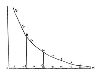
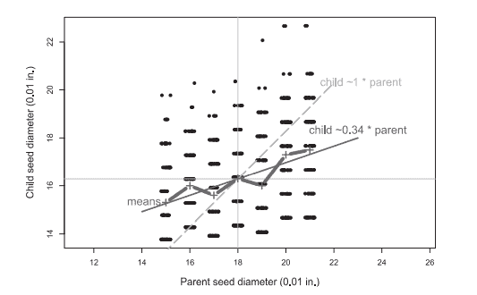
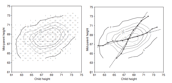
Galton’s next step on the problem of filial correlation and regression turned out to be one of the most important in the history of statistics. In 1886, he published a paper titled “Regression Towards Mediocrity in Hereditary Stature” containing the table shown in Figure 6.14. The table records the frequencies of the heights of 928 adult children born to 205 pairs of fathers and mothers, classified by the average height of their father and mother (“mid-parent” height).$^{22}$

If you look at this table, you may see only a table of numbers with larger values in the middle and some dashes (meaning 0 ) in the upper left, and bottom right corners. But for Galton, it was something he could compute with, both in his mind’s eye and on paper.

I found it hard at first to catch the full significance of the entries in the table, which had curious relations that were very interesting to investigate. They came out distinctly when I “smoothed” the entries by writing at each intersection of a horizontal column with a vertical one, the sum of the entries in the four adjacent squares, and using these to work upon. (Galton, 1886, p. 254)

Consequently, Galton first smoothed the numbers in this table, which he did by the simple step of summing (or averaging) each set of four adjacent cells. We can imagine that he wrote that average number larger in red ink, exactly at the intersection of these four cells. When he had completed this task, we can imagine him standing above the table with a different pen and trying to connect the dots-to draw curves, joining the points of approximately equal frequency. We tried to reproduce these steps in Figure 6.15, except that we did the last step mechanically, using a computer algorithm, whereas Galton probably did it by eye and brain, in the manner of Herschel, with the aim that the resulting curves should be gracefully smooth.

数据可视化代考

统计代写|数据可视化代写数据可视化代考|Francis Galton和相关性的思想

Francis Galton[1822-1911]是第一个使用实际数据以图形形式展示纯经验二元关系的人之一，他的工作涉及性状的遗传力问题。他从展示人的身体特征(头围和身高)之间的关系，或父母和他们的后代之间的关系的图表开始，作为一种研究特征的关联和遗传的手段:高个子的人的头比普通人大吗?个子高的父母生的孩子比一般人高吗?

从他的图表中检查和计算，他发现了一种被他称为“趋均数回归”的现象，他对这些问题的研究可以被认为是现代统计方法的基础。他从这些图表中得出的见解带来了更多:相关性和线性回归的思想;二元正态分布;并最终对几乎所有的经典线性统计模型(方差分析、多元回归等)进行了分析。已知最早的例子是高尔顿笔记本上的头围与身高对比图(约1874年)。“特殊特性”如图6.11所示。${ }^{16}$在这张手绘的图表中，身高的间隔水平地与头围垂直地对比。主体中的条目是类间隔对的计数。Galton将身高和头围的总数包括在右侧和底部的空白中，并画出光滑的曲线来表示它们的频率分布。这张图表的概念起源是表格而不是图形，这可以从两个变量的最小值显示在左上角(第一行和第一列)，而不是显示在右下角(在图形中更自然)这一事实中看出。有人可能会说，高尔顿对二元关系的图形表示既不是真实的数据散点图，也不是真实的数据散点图，就像今天所使用的那样。它们之所以少，是因为乍一看，它们不过是一些带有图形注释的表格。更重要的是，他把这些作为计算和推理的工具。${ }^{17} \mathrm{He}$这样做是因为他所寻求的回归线最初被定义为垂直变量$y$的平均值的轨迹，而水平变量$x$的变化是$^{18}$(我们现在认为是条件均值函数$\mathcal{E}(y \mid x)$)，因此至少需要将$x$变量分组到类间隔中。高尔顿对这些数据的显示，本质上是对这些表格的图形复制，使用计数符号$(/, / /, / / /, \ldots)$或数字来表示每个细胞的频率——1972年，普林斯顿大学的博学家约翰·杜克(John Tukey)将其称为“半图形显示”，使它们成为视觉上的嵌合体:部分是表格，部分是图表

统计代写|数据可视化代写数据可视化代考|高尔顿椭圆洞察

高尔顿在子相关和回归问题上的下一步被证明是统计史上最重要的一步。1886年，他发表了一篇题为《世袭身材向平庸的回归》的论文，其中包含了如图6.14所示的表格。该表格记录了205对父亲和母亲所生的928名成年子女的身高频率，并根据他们的父亲和母亲的平均身高(“中间父母”身高)进行了分类。$^{22}$

如果你看一下这个表格，你可能只会看到一个数字表，中间是较大的值，左上角和右下角有一些破折号(表示0)。但对高尔顿来说，这是他可以用脑子和纸来计算的东西

一开始我发现很难抓住表中条目的全部意义，它们之间有着非常有趣的关系，值得研究。当我在水平列和垂直列的每一个交叉点上写下四个相邻方格中条目的和，并使用这些条目来“平滑”条目时，它们明显地显现出来。(高尔顿，1886,p. 254)

因此，高尔顿首先平滑了该表中的数字，他通过简单的步骤，对每组相邻的四个单元格进行求和(或平均)。我们可以想象他用红墨水把平均数写大了，正好在这四个单元格的交点处。当他完成这项任务后，我们可以想象他站在桌子上方，拿着另一支笔，试图把点连接起来——画曲线，把频率大致相等的点连接起来。我们试着在图6.15中重现这些步骤，除了最后一步是机械地用计算机算法完成的，而高尔顿可能是用眼睛和大脑，以赫歇尔的方式完成的，目的是要得到优雅光滑的曲线

统计代写请认准statistics-lab™. statistics-lab™为您的留学生涯保驾护航。

金融工程代写

金融工程是使用数学技术来解决金融问题。金融工程使用计算机科学、统计学、经济学和应用数学领域的工具和知识来解决当前的金融问题，以及设计新的和创新的金融产品。

非参数统计代写

非参数统计指的是一种统计方法，其中不假设数据来自于由少数参数决定的规定模型；这种模型的例子包括正态分布模型和线性回归模型。

广义线性模型代考

广义线性模型（GLM）归属统计学领域，是一种应用灵活的线性回归模型。该模型允许因变量的偏差分布有除了正态分布之外的其它分布。

术语 广义线性模型（GLM）通常是指给定连续和/或分类预测因素的连续响应变量的常规线性回归模型。它包括多元线性回归，以及方差分析和方差分析（仅含固定效应）。

有限元方法代写

有限元方法（FEM）是一种流行的方法，用于数值解决工程和数学建模中出现的微分方程。典型的问题领域包括结构分析、传热、流体流动、质量运输和电磁势等传统领域。

有限元是一种通用的数值方法，用于解决两个或三个空间变量的偏微分方程（即一些边界值问题）。为了解决一个问题，有限元将一个大系统细分为更小、更简单的部分，称为有限元。这是通过在空间维度上的特定空间离散化来实现的，它是通过构建对象的网格来实现的：用于求解的数值域，它有有限数量的点。边界值问题的有限元方法表述最终导致一个代数方程组。该方法在域上对未知函数进行逼近。[1] 然后将模拟这些有限元的简单方程组合成一个更大的方程系统，以模拟整个问题。然后，有限元通过变化微积分使相关的误差函数最小化来逼近一个解决方案。

tatistics-lab作为专业的留学生服务机构，多年来已为美国、英国、加拿大、澳洲等留学热门地的学生提供专业的学术服务，包括但不限于Essay代写，Assignment代写，Dissertation代写，Report代写，小组作业代写，Proposal代写，Paper代写，Presentation代写，计算机作业代写，论文修改和润色，网课代做，exam代考等等。写作范围涵盖高中，本科，研究生等海外留学全阶段，辐射金融，经济学，会计学，审计学，管理学等全球99%专业科目。写作团队既有专业英语母语作者，也有海外名校硕博留学生，每位写作老师都拥有过硬的语言能力，专业的学科背景和学术写作经验。我们承诺100%原创，100%专业，100%准时，100%满意。

随机分析代写

随机微积分是数学的一个分支，对随机过程进行操作。它允许为随机过程的积分定义一个关于随机过程的一致的积分理论。这个领域是由日本数学家伊藤清在第二次世界大战期间创建并开始的。

时间序列分析代写

随机过程，是依赖于参数的一组随机变量的全体，参数通常是时间。 随机变量是随机现象的数量表现，其时间序列是一组按照时间发生先后顺序进行排列的数据点序列。通常一组时间序列的时间间隔为一恒定值（如1秒，5分钟，12小时，7天，1年），因此时间序列可以作为离散时间数据进行分析处理。研究时间序列数据的意义在于现实中，往往需要研究某个事物其随时间发展变化的规律。这就需要通过研究该事物过去发展的历史记录，以得到其自身发展的规律。

回归分析代写

多元回归分析渐进（Multiple Regression Analysis Asymptotics）属于计量经济学领域，主要是一种数学上的统计分析方法，可以分析复杂情况下各影响因素的数学关系，在自然科学、社会和经济学等多个领域内应用广泛。

MATLAB代写

MATLAB 是一种用于技术计算的高性能语言。它将计算、可视化和编程集成在一个易于使用的环境中，其中问题和解决方案以熟悉的数学符号表示。典型用途包括：数学和计算算法开发建模、仿真和原型制作数据分析、探索和可视化科学和工程图形应用程序开发，包括图形用户界面构建MATLAB 是一个交互式系统，其基本数据元素是一个不需要维度的数组。这使您可以解决许多技术计算问题，尤其是那些具有矩阵和向量公式的问题，而只需用 C 或 Fortran 等标量非交互式语言编写程序所需的时间的一小部分。MATLAB 名称代表矩阵实验室。MATLAB 最初的编写目的是提供对由 LINPACK 和 EISPACK 项目开发的矩阵软件的轻松访问，这两个项目共同代表了矩阵计算软件的最新技术。MATLAB 经过多年的发展，得到了许多用户的投入。在大学环境中，它是数学、工程和科学入门和高级课程的标准教学工具。在工业领域，MATLAB 是高效研究、开发和分析的首选工具。MATLAB 具有一系列称为工具箱的特定于应用程序的解决方案。对于大多数 MATLAB 用户来说非常重要，工具箱允许您学习和应用专业技术。工具箱是 MATLAB 函数（M 文件）的综合集合，可扩展 MATLAB 环境以解决特定类别的问题。可用工具箱的领域包括信号处理、控制系统、神经网络、模糊逻辑、小波、仿真等。

R语言代写	问卷设计与分析代写
PYTHON代写	回归分析与线性模型代写
MATLAB代写	方差分析与试验设计代写
STATA代写	机器学习/统计学习代写
SPSS代写	计量经济学代写
EVIEWS代写	时间序列分析代写
EXCEL代写	深度学习代写
SQL代写	各种数据建模与可视化代写

如果你也在 怎样代写数据可视化Data visualization这个学科遇到相关的难题，请随时右上角联系我们的24/7代写客服。

数据可视化是将信息转化为视觉背景的做法，如地图或图表，使数据更容易被人脑理解并从中获得洞察力。数据可视化的主要目标是使其更容易在大型数据集中识别模式、趋势和异常值。

statistics-lab™ 为您的留学生涯保驾护航 在代写数据可视化Data visualization方面已经树立了自己的口碑, 保证靠谱, 高质且原创的统计Statistics代写服务。我们的专家在代写数据可视化Data visualization代写方面经验极为丰富，各种代写数据可视化Data visualization相关的作业也就用不着说。

我们提供的数据可视化Data visualization及其相关学科的代写，服务范围广, 其中包括但不限于:

• Statistical Inference 统计推断
• Statistical Computing 统计计算
• Advanced Probability Theory 高等概率论
• Advanced Mathematical Statistics 高等数理统计学
• (Generalized) Linear Models 广义线性模型
• Statistical Machine Learning 统计机器学习
• Longitudinal Data Analysis 纵向数据分析
• Foundations of Data Science 数据科学基础

统计代写|数据可视化代写Data visualization代考|John Herschel and the Orbits of Twin Stars

In the hundred years from 1750 to 1850 , during which most of the modern graphic forms were invented, fundamentally important problems of measurement attracted the best mathematical minds, including Euler, Laplace,

Legendre, Newton, and Gauss, and led to the inventions of calculus, least squares, curve fitting, and interpolation. ${ }^8$ In these scientific and mathematical domains, graphs had begun to play an increasing role in the explanation of scientific phenomena, as we described earlier in the case of Johann Lambert.
Among this work, we find the remarkable paper of Sir John Frederick W. Herschel [1792-1871], On the Investigation of the Orbits of Revolving Double Stars, which he read to the Royal Astronomical Society on January 13, 1832, and published the next year. Double stars had long played a particularly important role in astrophysics because they provided the best means to measure stellar masses and sizes, and this paper was prepared as andendum to another 1833 paper, in which Herschel had meticulously cataloged observations on the orbits of 364 double stars.

The printed paper refers to four figures, presented at the meeting. Alas, the version printed in the Memoirs of the Royal Astronomical Society did not include them, presumably owing to the cost of engraving. Herschel noted, “The original charts and figures which accompanied the paper being all deposited with the Society.” These might have been lost to historians, but Thomas Hankins discovered copies of them in research for his insightful 2006 paper on Herschel’s graphical method.

To see why Herschel’s paper is remarkable, we must follow his exposition of the goals, the construction of scatterplots, and the idea of visual smoothing to produce a more satisfactory solution for parameters of the orbits of double stars than were available by analytic methods.

统计代写|数据可视化代写Data visualization代考|Herschel’s Graphical Impact Factor

The critical reader may object, thinking that Herschel’s graphical method, as ingenious as it might be, did not produce true scatterplots in the modern sense because the horizontal axis in Figure $6.9$ is time rather than a separate variable. Thus one might argue that all we have is another time-series graph,so priority really belongs to Playfair, or further back, to Lambert, who stated the essential ideas. On the surface this is true.

But it’s only true on the surface. We argue that a close and appreciative reading of Herschel’s description of his graphical method can, at the very least, be considered a true innovation in visual thinking, worthy of note in the present account. More importantly, Herschel’s true objective was to calculate the parameters of the orbits of twin stars based on the relation between position angle and separation distance; the use of time appears in the graph as a proxy or indirect means to overcome the scant observations and perhaps extravagant errors in the data on separation distance.

Yet Herschel’s graphical development of calculation based on a scatterplot attracted little attention outside the field of astronomy, where his results were widely hailed as groundbreaking in the Royal Astronomical Society. But this notice was for his scientific achievement rather than for his contribution of a graphical method, which scientists probably rightly considered just a means to an end.

It took another 30-50 years for graphical methods to be fully welcomed into the family of data-based scientific explanation, and seen as something more than mere illustrations. This change is best recorded in presentations at the Silver Jubilee of the Royal Statistical Society in 1885 . Even at that time, most British statisticians still considered themselves “statists”, mere recorders of statistical facts in numerical tables; but “graphists” had finally been invited to the party.

On June 23, the influential British economist Alfred Marshall [1842-1924] addressed the attendees on the benefits of the graphic method, a radical departure for a statist. His French counterpart Émile Levasseur [1828-1911] presented a survey of the wide variety of graphs and statistical maps then in use. Yet even then, the scientific work of Lambert and Herschel, and the concept of the scatterplot as a new graphical form remained largely unknown. This would soon change with Francis Galton.

数据可视化代考

统计代写|数据可视化代写数据可视化代考|约翰·赫歇尔和双星轨道

从1750年到1850年的几百年里，在这段时间里，大多数现代图形形式被发明出来，最重要的测量问题吸引了最优秀的数学头脑，包括欧拉，拉普拉斯

勒让德，牛顿和高斯，并导致了微积分，最小二乘，曲线拟合和插值的发明。${ }^8$在这些科学和数学领域，图已经开始在解释科学现象方面发挥越来越大的作用，正如我们之前在约翰·兰伯特的例子中所描述的那样。在这些著作中，我们发现了约翰·弗雷德里克·赫歇尔爵士[1792-1871]的杰出论文《关于旋转双星轨道的研究》，他于1832年1月13日向皇家天文学会宣读了这篇论文，并于次年发表。双星长期以来一直在天体物理学中发挥着特别重要的作用，因为它们提供了测量恒星质量和大小的最佳手段。这篇论文是1833年另一篇论文的附录，在那篇论文中，赫舍尔对364颗双星的轨道观测进行了细致入微的编目

印刷的文件是指在会议上提出的四个数字。可惜的是，印在《皇家天文学会回忆录》上的版本没有包括它们，大概是由于雕刻成本的原因。赫歇尔说:“随论文而来的原始图表和数据都存放在协会。”历史学家可能已经遗失了它们，但托马斯·汉金斯(Thomas Hankins)在2006年发表的关于赫歇尔图解法的论文中发现了它们的副本

要了解为什么Herschel的论文是卓越的，我们必须遵循他对目标的阐述，散点图的构建，以及视觉平滑的思想，以产生一个比解析方法更令人满意的双星轨道参数的解

统计代写|数据可视化代写数据可视化代考|赫歇尔的图形影响因子

挑剔的读者可能会反对，认为赫歇尔的图解方法，尽管可能很巧妙，但并没有产生现代意义上真正的散点图，因为图$6.9$中的横轴是时间，而不是一个单独的变量。因此，有人可能会说，我们所拥有的只是另一个时间序列图，所以优先级实际上属于Playfair，或者更早以前的Lambert，他阐述了基本理念。从表面上看，这是正确的

但这只是表面上的事实。我们认为，仔细阅读赫歇尔对他的图解方法的描述，至少可以被认为是视觉思维的真正创新，在目前的叙述中值得注意。更重要的是，赫歇尔的真正目的是根据位置角和分离距离的关系计算出双星轨道的参数;在图中，时间的使用作为一种代理或间接手段，以克服分离距离数据中观测的不足和可能存在的巨大误差

然而，赫歇尔基于散点图的计算图形化发展在天文学领域之外几乎没有引起注意，他的结果在皇家天文学会被广泛称赞为开创性的。但是，这个通告是为了表彰他的科学成就，而不是表彰他对图形方法的贡献，科学家们可能正确地认为图形方法只是达到目的的一种手段

又过了30-50年，图形方法才被完全纳入基于数据的科学解释的大家庭，并被视为不仅仅是插图的东西。这一变化在1885年皇家统计学会银禧庆典上的演讲中得到了最好的记录。即使在那个时候，大多数英国统计学家仍然认为自己是“统计学家”，仅仅是用数字表格记录统计事实;但是“绘图家”最终还是被邀请参加了这个聚会

6月23日，有影响力的英国经济学家阿尔弗雷德·马歇尔(Alfred Marshall, 1842-1924)向与会者发表了关于图表方法的好处的演讲，这是对中央集权主义者的一种激进的背离。他的法国同行Émile Levasseur[1828-1911]对当时使用的各种各样的图表和统计地图进行了调查。然而，即使在那时，兰伯特和赫歇尔的科学工作，以及散点图作为一种新的图形形式的概念，在很大程度上仍然是未知的。弗朗西斯·高尔顿很快改变了这种情况

统计代写请认准statistics-lab™. statistics-lab™为您的留学生涯保驾护航。

金融工程代写

金融工程是使用数学技术来解决金融问题。金融工程使用计算机科学、统计学、经济学和应用数学领域的工具和知识来解决当前的金融问题，以及设计新的和创新的金融产品。

非参数统计代写

非参数统计指的是一种统计方法，其中不假设数据来自于由少数参数决定的规定模型；这种模型的例子包括正态分布模型和线性回归模型。

广义线性模型代考

广义线性模型（GLM）归属统计学领域，是一种应用灵活的线性回归模型。该模型允许因变量的偏差分布有除了正态分布之外的其它分布。

术语 广义线性模型（GLM）通常是指给定连续和/或分类预测因素的连续响应变量的常规线性回归模型。它包括多元线性回归，以及方差分析和方差分析（仅含固定效应）。

有限元方法代写

有限元方法（FEM）是一种流行的方法，用于数值解决工程和数学建模中出现的微分方程。典型的问题领域包括结构分析、传热、流体流动、质量运输和电磁势等传统领域。

有限元是一种通用的数值方法，用于解决两个或三个空间变量的偏微分方程（即一些边界值问题）。为了解决一个问题，有限元将一个大系统细分为更小、更简单的部分，称为有限元。这是通过在空间维度上的特定空间离散化来实现的，它是通过构建对象的网格来实现的：用于求解的数值域，它有有限数量的点。边界值问题的有限元方法表述最终导致一个代数方程组。该方法在域上对未知函数进行逼近。[1] 然后将模拟这些有限元的简单方程组合成一个更大的方程系统，以模拟整个问题。然后，有限元通过变化微积分使相关的误差函数最小化来逼近一个解决方案。

tatistics-lab作为专业的留学生服务机构，多年来已为美国、英国、加拿大、澳洲等留学热门地的学生提供专业的学术服务，包括但不限于Essay代写，Assignment代写，Dissertation代写，Report代写，小组作业代写，Proposal代写，Paper代写，Presentation代写，计算机作业代写，论文修改和润色，网课代做，exam代考等等。写作范围涵盖高中，本科，研究生等海外留学全阶段，辐射金融，经济学，会计学，审计学，管理学等全球99%专业科目。写作团队既有专业英语母语作者，也有海外名校硕博留学生，每位写作老师都拥有过硬的语言能力，专业的学科背景和学术写作经验。我们承诺100%原创，100%专业，100%准时，100%满意。

随机分析代写

随机微积分是数学的一个分支，对随机过程进行操作。它允许为随机过程的积分定义一个关于随机过程的一致的积分理论。这个领域是由日本数学家伊藤清在第二次世界大战期间创建并开始的。

时间序列分析代写

随机过程，是依赖于参数的一组随机变量的全体，参数通常是时间。 随机变量是随机现象的数量表现，其时间序列是一组按照时间发生先后顺序进行排列的数据点序列。通常一组时间序列的时间间隔为一恒定值（如1秒，5分钟，12小时，7天，1年），因此时间序列可以作为离散时间数据进行分析处理。研究时间序列数据的意义在于现实中，往往需要研究某个事物其随时间发展变化的规律。这就需要通过研究该事物过去发展的历史记录，以得到其自身发展的规律。

回归分析代写

多元回归分析渐进（Multiple Regression Analysis Asymptotics）属于计量经济学领域，主要是一种数学上的统计分析方法，可以分析复杂情况下各影响因素的数学关系，在自然科学、社会和经济学等多个领域内应用广泛。

MATLAB代写

MATLAB 是一种用于技术计算的高性能语言。它将计算、可视化和编程集成在一个易于使用的环境中，其中问题和解决方案以熟悉的数学符号表示。典型用途包括：数学和计算算法开发建模、仿真和原型制作数据分析、探索和可视化科学和工程图形应用程序开发，包括图形用户界面构建MATLAB 是一个交互式系统，其基本数据元素是一个不需要维度的数组。这使您可以解决许多技术计算问题，尤其是那些具有矩阵和向量公式的问题，而只需用 C 或 Fortran 等标量非交互式语言编写程序所需的时间的一小部分。MATLAB 名称代表矩阵实验室。MATLAB 最初的编写目的是提供对由 LINPACK 和 EISPACK 项目开发的矩阵软件的轻松访问，这两个项目共同代表了矩阵计算软件的最新技术。MATLAB 经过多年的发展，得到了许多用户的投入。在大学环境中，它是数学、工程和科学入门和高级课程的标准教学工具。在工业领域，MATLAB 是高效研究、开发和分析的首选工具。MATLAB 具有一系列称为工具箱的特定于应用程序的解决方案。对于大多数 MATLAB 用户来说非常重要，工具箱允许您学习和应用专业技术。工具箱是 MATLAB 函数（M 文件）的综合集合，可扩展 MATLAB 环境以解决特定类别的问题。可用工具箱的领域包括信号处理、控制系统、神经网络、模糊逻辑、小波、仿真等。

R语言代写	问卷设计与分析代写
PYTHON代写	回归分析与线性模型代写
MATLAB代写	方差分析与试验设计代写
STATA代写	机器学习/统计学习代写
SPSS代写	计量经济学代写
EVIEWS代写	时间序列分析代写
EXCEL代写	深度学习代写
SQL代写	各种数据建模与可视化代写

如果你也在 怎样代写数据可视化Data visualization这个学科遇到相关的难题，请随时右上角联系我们的24/7代写客服。

数据可视化是将信息转化为视觉背景的做法，如地图或图表，使数据更容易被人脑理解并从中获得洞察力。数据可视化的主要目标是使其更容易在大型数据集中识别模式、趋势和异常值。

statistics-lab™ 为您的留学生涯保驾护航 在代写数据可视化Data visualization方面已经树立了自己的口碑, 保证靠谱, 高质且原创的统计Statistics代写服务。我们的专家在代写数据可视化Data visualization代写方面经验极为丰富，各种代写数据可视化Data visualization相关的作业也就用不着说。

我们提供的数据可视化Data visualization及其相关学科的代写，服务范围广, 其中包括但不限于:

• Statistical Inference 统计推断
• Statistical Computing 统计计算
• Advanced Probability Theory 高等概率论
• Advanced Mathematical Statistics 高等数理统计学
• (Generalized) Linear Models 广义线性模型
• Statistical Machine Learning 统计机器学习
• Longitudinal Data Analysis 纵向数据分析
• Foundations of Data Science 数据科学基础

统计代写|数据可视化代写Data visualization代考|The Broad Street Pump

Snow’s opportunity to test his theory came with the new eruption that began toward the end of August in 1854. His celebrated 1855 report, On the Mode of Communication of Cholera, ${ }^{16}$ describes it dramatically:
The most terrible outbreak of cholera which ever occurred in this kingdom, is probably that which took place in Broad Street, Golden Square, and the adjoining streets, a few weeks ago. Within two hundred and fifty yards of the spot where Cambridge Street joins Broad Street, there were upwards of five hundred fatal attacks of cholera in ten days. The mortality in this limited area probably equals any that was ever caused in this country, even by the plague; and it was much more sudden, as the greater number of cases terminated in a few hours. (p. 38)

The full story of Snow’s discovery of the waterborne cause of cholera has been told in rich detail many times, by medical historians ${ }^{17}$ and cartographers, ${ }^{18}$ and it was brought to the attention of statisticians and those interested in the history of data visualization by Edward Tufte. ${ }^{19}$

The short, if slightly apocryphal, version of this story is that, during the outbreak of cholera in Soho in 1854, Snow created a dot map of the locations of deaths and immediately noticed that they clustered on Broad Street, near the site of one of the public pumps from which residents drew their water. This narrative continues: Snow recognized that cases of death were strongly associated with drinking water from this pump. He petitioned the Board of Guardians of St. James Parish to remove the pump handle, whereupon the cholera epidemic subsided.

统计代写|数据可视化代写Data visualization代考|The Neighborhoods Map

The version of Snow’s map shown in Figure $4.7$ is the most famous, but a second version is more interesting graphically and scientifically. The Cholera Inquiry Committee, appointed by the Vestry of St. James, submitted its report on July 25, 1855. ${ }^{22}$ The section titled “Dr. Snow’s Report” contained a new map that attempted a more detailed and direct visual analysis of the association of death with the Broad Street pump.

This new map, shown in Figure 4.8, states and tests a geospatial hypothesis: people are most likely to draw their water from the nearest pump (by walking distance). The outlined region in this map “shews the various points which have been found by careful measurement to be at an equal distance by the nearest road from the pump in Broad Street and the surrounding pumps.” 23

If the source of the outbreak was indeed the Broad Street pump, one should expect to find the highest concentration of deaths within this area, and also a low prevalence outside it. He stated his conclusion as “it will be observed that the deaths either very much diminish, or cease altogether, at every point where it becomes decidedly nearer to send to another pump than to the one in Broad street.” 24

The final explanation for the source of the outbreak came slightly later, through the work of Reverend Henry Whitehead, the curate at a local church and a member of the Cholera Inquiry Committee. He identified the first (“index”) case as the death of a five-month-old infant, Frances Lewis, whose family lived at 40 Broad Street, immediately adjacent to the pump. When severe diarrhea struck the child, her mother, Sarah Lewis, soaked the diapers and emptied the pails into the cesspool at the front of their house, only three feet from the well. Unfortunately, the cesspool walls had decayed and the effluent flowed directly into the pump well. Thomas Lewis, the baby’s father and a local constable, suffered a fatal attack of the disease on September 8, the same day that the pump handle was removed.

数据可视化代考

统计代写|数据可视化代写Data visualization代考|The Broad Street Pump

斯诺检验他的理论的机会来自于 1854 年 8 月底开始的新喷发。他在 1855 年的著名报告《霍乱的传播方式》，16戏剧性地描述了它：
这个王国曾经发生过的最可怕的霍乱爆发，可能是几周前发生在布罗德街、黄金广场和毗邻街道的那次。在剑桥街与布罗德街交汇处的 250 码范围内，十天内发生了超过 500 起致命的霍乱袭击。这个有限地区的死亡人数可能与这个国家曾经造成的死亡人数相等，即使是瘟疫也是如此；而且它更加突然，因为更多的案件在几个小时内就结束了。（第 38 页）

医学历史学家多次详细讲述了斯诺发现霍乱水源性病因的全部故事17和制图师，18爱德华·塔夫特 (Edward Tufte) 引起了统计学家和那些对数据可视化历史感兴趣的人的注意。19

这个故事的简短版本是，1854 年苏荷区霍乱爆发期间，斯诺创建了一张死亡地点的点图，并立即注意到他们聚集在布罗德街，靠近一个居民抽水的公共水泵。这种叙述仍在继续：斯诺认识到死亡病例与该泵的饮用水密切相关。他请求圣詹姆斯教区的监护委员会拆除泵把手，霍乱疫情随即消退。

统计代写|数据可视化代写Data visualization代考|The Neighborhoods Map

雪诺的版本如图4.7是最著名的，但第二个版本在图形和科学上更有趣。由圣詹姆斯教区任命的霍乱调查委员会于 1855 年 7 月 25 日提交了报告。22标题为“博士”的部分。斯诺的报告”包含一张新地图，试图对死亡与布罗德街水泵的关联进行更详细和直接的视觉分析。

这张新地图如图 4.8 所示，陈述并检验了一个地理空间假设：人们最有可能从最近的泵（步行距离）取水。这张地图中的轮廓区域“显示了通过仔细测量发现的各个点，距离 Broad Street 的泵和周围的泵最近的道路距离相等。” 23

如果爆发的源头确实是布罗德街的水泵，那么人们应该会发现该地区的死亡人数最高，而该地区以外的流行率也很低。他说他的结论是“可以观察到，死亡人数要么大大减少，要么完全停止，在每一个地方，与布罗德街的泵相比，泵送至另一台泵变得明显更近。” 24

通过当地教堂的牧师和霍乱调查委员会成员亨利怀特黑德牧师的工作，对爆发源头的最终解释来得稍晚一些。他确定第一个（“索引”）病例是一个五个月大的婴儿弗朗西斯·刘易斯（Frances Lewis）的死亡，她的家人住在布罗德街 40 号，紧邻水泵。当孩子出现严重腹泻时，她的母亲莎拉·刘易斯（Sarah Lewis）浸湿了尿布，并将桶倒进了他们家门前的污水池，距离井只有三英尺。不幸的是，污水池的墙壁已经腐烂，污水直接流入泵井。婴儿的父亲和当地警察托马斯·刘易斯于 9 月 8 日患上了致命的疾病，就在泵把手被拆除的同一天。

统计代写请认准statistics-lab™. statistics-lab™为您的留学生涯保驾护航。

金融工程代写

金融工程是使用数学技术来解决金融问题。金融工程使用计算机科学、统计学、经济学和应用数学领域的工具和知识来解决当前的金融问题，以及设计新的和创新的金融产品。

非参数统计代写

非参数统计指的是一种统计方法，其中不假设数据来自于由少数参数决定的规定模型；这种模型的例子包括正态分布模型和线性回归模型。

广义线性模型代考

广义线性模型（GLM）归属统计学领域，是一种应用灵活的线性回归模型。该模型允许因变量的偏差分布有除了正态分布之外的其它分布。

术语 广义线性模型（GLM）通常是指给定连续和/或分类预测因素的连续响应变量的常规线性回归模型。它包括多元线性回归，以及方差分析和方差分析（仅含固定效应）。

有限元方法代写

有限元方法（FEM）是一种流行的方法，用于数值解决工程和数学建模中出现的微分方程。典型的问题领域包括结构分析、传热、流体流动、质量运输和电磁势等传统领域。

有限元是一种通用的数值方法，用于解决两个或三个空间变量的偏微分方程（即一些边界值问题）。为了解决一个问题，有限元将一个大系统细分为更小、更简单的部分，称为有限元。这是通过在空间维度上的特定空间离散化来实现的，它是通过构建对象的网格来实现的：用于求解的数值域，它有有限数量的点。边界值问题的有限元方法表述最终导致一个代数方程组。该方法在域上对未知函数进行逼近。[1] 然后将模拟这些有限元的简单方程组合成一个更大的方程系统，以模拟整个问题。然后，有限元通过变化微积分使相关的误差函数最小化来逼近一个解决方案。

tatistics-lab作为专业的留学生服务机构，多年来已为美国、英国、加拿大、澳洲等留学热门地的学生提供专业的学术服务，包括但不限于Essay代写，Assignment代写，Dissertation代写，Report代写，小组作业代写，Proposal代写，Paper代写，Presentation代写，计算机作业代写，论文修改和润色，网课代做，exam代考等等。写作范围涵盖高中，本科，研究生等海外留学全阶段，辐射金融，经济学，会计学，审计学，管理学等全球99%专业科目。写作团队既有专业英语母语作者，也有海外名校硕博留学生，每位写作老师都拥有过硬的语言能力，专业的学科背景和学术写作经验。我们承诺100%原创，100%专业，100%准时，100%满意。

随机分析代写

随机微积分是数学的一个分支，对随机过程进行操作。它允许为随机过程的积分定义一个关于随机过程的一致的积分理论。这个领域是由日本数学家伊藤清在第二次世界大战期间创建并开始的。

时间序列分析代写

随机过程，是依赖于参数的一组随机变量的全体，参数通常是时间。 随机变量是随机现象的数量表现，其时间序列是一组按照时间发生先后顺序进行排列的数据点序列。通常一组时间序列的时间间隔为一恒定值（如1秒，5分钟，12小时，7天，1年），因此时间序列可以作为离散时间数据进行分析处理。研究时间序列数据的意义在于现实中，往往需要研究某个事物其随时间发展变化的规律。这就需要通过研究该事物过去发展的历史记录，以得到其自身发展的规律。

回归分析代写

多元回归分析渐进（Multiple Regression Analysis Asymptotics）属于计量经济学领域，主要是一种数学上的统计分析方法，可以分析复杂情况下各影响因素的数学关系，在自然科学、社会和经济学等多个领域内应用广泛。

MATLAB代写

MATLAB 是一种用于技术计算的高性能语言。它将计算、可视化和编程集成在一个易于使用的环境中，其中问题和解决方案以熟悉的数学符号表示。典型用途包括：数学和计算算法开发建模、仿真和原型制作数据分析、探索和可视化科学和工程图形应用程序开发，包括图形用户界面构建MATLAB 是一个交互式系统，其基本数据元素是一个不需要维度的数组。这使您可以解决许多技术计算问题，尤其是那些具有矩阵和向量公式的问题，而只需用 C 或 Fortran 等标量非交互式语言编写程序所需的时间的一小部分。MATLAB 名称代表矩阵实验室。MATLAB 最初的编写目的是提供对由 LINPACK 和 EISPACK 项目开发的矩阵软件的轻松访问，这两个项目共同代表了矩阵计算软件的最新技术。MATLAB 经过多年的发展，得到了许多用户的投入。在大学环境中，它是数学、工程和科学入门和高级课程的标准教学工具。在工业领域，MATLAB 是高效研究、开发和分析的首选工具。MATLAB 具有一系列称为工具箱的特定于应用程序的解决方案。对于大多数 MATLAB 用户来说非常重要，工具箱允许您学习和应用专业技术。工具箱是 MATLAB 函数（M 文件）的综合集合，可扩展 MATLAB 环境以解决特定类别的问题。可用工具箱的领域包括信号处理、控制系统、神经网络、模糊逻辑、小波、仿真等。

R语言代写	问卷设计与分析代写
PYTHON代写	回归分析与线性模型代写
MATLAB代写	方差分析与试验设计代写
STATA代写	机器学习/统计学习代写
SPSS代写	计量经济学代写
EVIEWS代写	时间序列分析代写
EXCEL代写	深度学习代写
SQL代写	各种数据建模与可视化代写

如果你也在 怎样代写数据可视化Data visualization这个学科遇到相关的难题，请随时右上角联系我们的24/7代写客服。

数据可视化是将信息转化为视觉背景的做法，如地图或图表，使数据更容易被人脑理解并从中获得洞察力。数据可视化的主要目标是使其更容易在大型数据集中识别模式、趋势和异常值。

statistics-lab™ 为您的留学生涯保驾护航 在代写数据可视化Data visualization方面已经树立了自己的口碑, 保证靠谱, 高质且原创的统计Statistics代写服务。我们的专家在代写数据可视化Data visualization代写方面经验极为丰富，各种代写数据可视化Data visualization相关的作业也就用不着说。

我们提供的数据可视化Data visualization及其相关学科的代写，服务范围广, 其中包括但不限于:

• Statistical Inference 统计推断
• Statistical Computing 统计计算
• Advanced Probability Theory 高等概率论
• Advanced Mathematical Statistics 高等数理统计学
• (Generalized) Linear Models 广义线性模型
• Statistical Machine Learning 统计机器学习
• Longitudinal Data Analysis 纵向数据分析
• Foundations of Data Science 数据科学基础

统计代写|数据可视化代写Data visualization代考|The Transcendent Effect of Water

Farr was certainly meticulous in evaluating the impact of potential causes on mortality from cholera. But he lacked an effective method for doing so, even for one potential cause, and the idea of accounting for the combination of several causes stretched him to the limit. His general method was to prepare tables of cholera mortality in the districts of London, broken down and averaged over classes of a possible explanatory variable.

For example, Farr divided the 38 districts into the 19 highest and 19 lowest values on other variables and calculated the ratio of cholera mortality for each; elevation had the largest ratio (3:1), while all other variables showed smaller ratios (e.g., 2.1:1 for house values). Having hit on elevation above the Thames as his principal cause, he prepared many other tables showing mortality by districts also in relation to density of the population, value of houses and shops, relief to the poor, and geographical features.

Figure $4.5$ illustrates the depth of this inquiry, in an ingenious semigraphic combination of small tables for each district overlaid on a schematic map of their spatial arrangement along the Thames. The tables show the numbers for elevation, cholera deaths, deaths from all causes, and population density, and identify the water companies supplying each district. Unfortunately, this lovely diagram concealed more than it revealed: the signal was there, but the wealth of detail provided too much noise.

It would later turn out that the direct cause of cholera could be traced to contamination of the water supply from which people drew. It was probably confusing that water was provided by nine water companies, as Farr shows in Figure 4.5, so he divided the registration districts into three groups based on the region along the Thames for their water supply: Thames, between Kew and Hammersmith bridges (western London), between Battersea and Waterloo bridges (central London), and districts that obtained their water from tributaries of the Thames (New River, Lea River, and Ravensbourne River).

统计代写|数据可视化代写Data visualization代考|John Snow on Cholera

Another terrible wave of cholera struck London toward the end of summer 1854, concentrated in the parish of St. James, Westminster (the present-day district of Soho). This time, a correct explanation of the cause would eventually be found with the aid of meticulous data collection, a map of disease incidence, keen medical detective work, and logical reasoning to rule out alternative explanations. It is useful to understand why John Snow succeeded while William Farr did not.

The physician John Snow [1813-1858] lived in the Soho district at the time of this new outbreak. He had been an eighteen-year-old medical assistant in Newcastle upon Tyne in 1831 when cholera first struck there with great loss of life. At the time of the second great epidemic, in 1848-1849, Snow observed the severity of the disease in his district. In 1849, in a two-part paper in the Medical Gazette and Times ${ }^{11}$ and a longer monograph ${ }^{12}$ he proposed that cholera was transmitted by water rather than through the air and passed from person to person through the intestinal discharges of the sick, either transmitted directly or entering the water supply.

Snow’s reasoning was entirely that of a clinician based on the form of pathology of the disease, rather than that of a statistician seeking associations with potential causal factors. Had cholera been an airborne disease, one would expect to see its effects in the lungs and then perhaps spread to others by respiratory discharge. But the disease clearly acted mainly in the gut, causing vomiting, intense diarrhea, and the massive dehydration that led to death. Whatever causal agent was responsible, it must have been something ingested rather than something inhaled.

William Farr was well aware of Snow’s theory when he wrote his 1852 report. ${ }^{13} \mathrm{He}$ described it quite politely but rejected Snow’s theory of the pathology of cholera. He could not understand any mechanism whereby something ingested by one individual could be passed to a larger community. To Farr, who was then considered the foremost authority on the outbreak and contagion of cholera, Snow’s contention of a single causal agent (some unknown poisonous matter, materies morbi) and a limited vector of transmission (water) was too circumscribed, too restrictive. Snow presented his argument and the evidence to support it as if ingestion and waterborne transmission could be the only causes; he also lacked the crucial data, either from a natural experiment or from direct knowledge of the water that cholera victims drank.

数据可视化代考

统计代写|数据可视化代写Data visualization代考|The Transcendent Effect of Water

法尔在评估潜在原因对霍乱死亡率的影响方面无疑是一丝不苟的。但是他缺乏有效的方法来做到这一点，即使是针对一个潜在的原因，而考虑多种原因的组合的想法使他走到了极限。他的一般方法是准备伦敦各地区的霍乱死亡率表，对可能的解释变量进行分类和平均。

例如，Farr 将 38 个地区划分为其他变量的 19 个最高值和 19 个最低值，并计算了每个地区的霍乱死亡率；海拔的比例最大（3:1），而所有其他变量的比例都较小（例如，房屋价值为 2.1:1）。将泰晤士河以上的海拔作为他的主要原因后，他准备了许多其他表格，显示各地区的死亡率，这些表格还与人口密度、房屋和商店的价值、对穷人的救济以及地理特征有关。

数字4.5展示了这项调查的深度，在每个地区的小桌子的巧妙半图形组合中，覆盖在泰晤士河沿岸空间布置的示意图上。这些表格显示了海拔、霍乱死亡人数、各种原因造成的死亡人数和人口密度，并确定了为每个地区供水的供水公司。不幸的是，这个可爱的图表隐藏的比它揭示的要多：信号在那里，但丰富的细节提供了太多的噪音。

后来发现，霍乱的直接原因可以追溯到人们取水的供水受到污染。正如法尔在图 4.5 中显示的那样，供水由九家供水公司提供可能令人困惑，因此他根据泰晤士河沿岸的供水地区将登记区分为三组：泰晤士河，在 Kew 和 Hammersmith 桥之间（西部伦敦），在巴特西和滑铁卢桥（伦敦市中心）之间，以及从泰晤士河支流（新河、利亚河和拉文斯伯恩河）取水的地区。

统计代写|数据可视化代写Data visualization代考|John Snow on Cholera

1854 年夏末，另一波可怕的霍乱袭击了伦敦，集中在威斯敏斯特的圣詹姆斯教区（现在的苏活区）。这一次，在细致的数据收集、疾病发病率地图、敏锐的医学侦探工作以及排除其他解释的逻辑推理的帮助下，最终将找到对原因的正确解释。理解为什么约翰·斯诺成功而威廉·法尔没有成功是很有用的。

在这次新的疫情爆发时，医生约翰·斯诺 [1813-1858] 住在苏荷区。1831 年，当霍乱首次袭击泰恩河畔纽卡斯尔时，他还是一名 18 岁的医疗助理，造成了巨大的生命损失。在 1848-1849 年第二次大流行病爆发时，斯诺观察了他所在地区疾病的严重程度。1849 年，在《医学公报》和《泰晤士报》的两篇论文中11和更长的专着12他提出，霍乱是通过水而不是空气传播的，并通过病人的肠道排泄物在人与人之间传播，要么直接传播，要么进入供水系统。

斯诺的推理完全是基于疾病病理学形式的临床医生的推理，而不是寻求与潜在因果因素关联的统计学家的推理。如果霍乱是一种空气传播的疾病，人们会期望看到它对肺部的影响，然后可能会通过呼吸道排出物传播给其他人。但这种疾病显然主要作用于肠道，导致呕吐、剧烈腹泻和导致死亡的大量脱水。无论病因是什么，它一定是被摄入的东西而不是被吸入的东西。

威廉·法尔 (William Farr) 在撰写 1852 年的报告时非常了解斯诺的理论。13H和描述得很客气，但拒绝了斯诺关于霍乱病理学的理论。他无法理解任何一种机制，可以将一个人摄入的东西传递给更大的社区。对于当时被认为是霍乱爆发和传染的最高权威的法尔来说，斯诺关于单一病原体（一些未知的有毒物质，即 morbi）和有限的传播媒介（水）的论点过于局限，过于严格。斯诺提出了他的论点和支持它的证据，好像摄入和水传播可能是唯一的原因；他还缺乏来自自然实验或直接了解霍乱受害者饮用的水的关键数据。

统计代写请认准statistics-lab™. statistics-lab™为您的留学生涯保驾护航。

金融工程代写

金融工程是使用数学技术来解决金融问题。金融工程使用计算机科学、统计学、经济学和应用数学领域的工具和知识来解决当前的金融问题，以及设计新的和创新的金融产品。

非参数统计代写

非参数统计指的是一种统计方法，其中不假设数据来自于由少数参数决定的规定模型；这种模型的例子包括正态分布模型和线性回归模型。

广义线性模型代考

广义线性模型（GLM）归属统计学领域，是一种应用灵活的线性回归模型。该模型允许因变量的偏差分布有除了正态分布之外的其它分布。

术语 广义线性模型（GLM）通常是指给定连续和/或分类预测因素的连续响应变量的常规线性回归模型。它包括多元线性回归，以及方差分析和方差分析（仅含固定效应）。

有限元方法代写

有限元方法（FEM）是一种流行的方法，用于数值解决工程和数学建模中出现的微分方程。典型的问题领域包括结构分析、传热、流体流动、质量运输和电磁势等传统领域。

有限元是一种通用的数值方法，用于解决两个或三个空间变量的偏微分方程（即一些边界值问题）。为了解决一个问题，有限元将一个大系统细分为更小、更简单的部分，称为有限元。这是通过在空间维度上的特定空间离散化来实现的，它是通过构建对象的网格来实现的：用于求解的数值域，它有有限数量的点。边界值问题的有限元方法表述最终导致一个代数方程组。该方法在域上对未知函数进行逼近。[1] 然后将模拟这些有限元的简单方程组合成一个更大的方程系统，以模拟整个问题。然后，有限元通过变化微积分使相关的误差函数最小化来逼近一个解决方案。

tatistics-lab作为专业的留学生服务机构，多年来已为美国、英国、加拿大、澳洲等留学热门地的学生提供专业的学术服务，包括但不限于Essay代写，Assignment代写，Dissertation代写，Report代写，小组作业代写，Proposal代写，Paper代写，Presentation代写，计算机作业代写，论文修改和润色，网课代做，exam代考等等。写作范围涵盖高中，本科，研究生等海外留学全阶段，辐射金融，经济学，会计学，审计学，管理学等全球99%专业科目。写作团队既有专业英语母语作者，也有海外名校硕博留学生，每位写作老师都拥有过硬的语言能力，专业的学科背景和学术写作经验。我们承诺100%原创，100%专业，100%准时，100%满意。

随机分析代写

随机微积分是数学的一个分支，对随机过程进行操作。它允许为随机过程的积分定义一个关于随机过程的一致的积分理论。这个领域是由日本数学家伊藤清在第二次世界大战期间创建并开始的。

时间序列分析代写

随机过程，是依赖于参数的一组随机变量的全体，参数通常是时间。 随机变量是随机现象的数量表现，其时间序列是一组按照时间发生先后顺序进行排列的数据点序列。通常一组时间序列的时间间隔为一恒定值（如1秒，5分钟，12小时，7天，1年），因此时间序列可以作为离散时间数据进行分析处理。研究时间序列数据的意义在于现实中，往往需要研究某个事物其随时间发展变化的规律。这就需要通过研究该事物过去发展的历史记录，以得到其自身发展的规律。

回归分析代写

多元回归分析渐进（Multiple Regression Analysis Asymptotics）属于计量经济学领域，主要是一种数学上的统计分析方法，可以分析复杂情况下各影响因素的数学关系，在自然科学、社会和经济学等多个领域内应用广泛。

MATLAB代写

MATLAB 是一种用于技术计算的高性能语言。它将计算、可视化和编程集成在一个易于使用的环境中，其中问题和解决方案以熟悉的数学符号表示。典型用途包括：数学和计算算法开发建模、仿真和原型制作数据分析、探索和可视化科学和工程图形应用程序开发，包括图形用户界面构建MATLAB 是一个交互式系统，其基本数据元素是一个不需要维度的数组。这使您可以解决许多技术计算问题，尤其是那些具有矩阵和向量公式的问题，而只需用 C 或 Fortran 等标量非交互式语言编写程序所需的时间的一小部分。MATLAB 名称代表矩阵实验室。MATLAB 最初的编写目的是提供对由 LINPACK 和 EISPACK 项目开发的矩阵软件的轻松访问，这两个项目共同代表了矩阵计算软件的最新技术。MATLAB 经过多年的发展，得到了许多用户的投入。在大学环境中，它是数学、工程和科学入门和高级课程的标准教学工具。在工业领域，MATLAB 是高效研究、开发和分析的首选工具。MATLAB 具有一系列称为工具箱的特定于应用程序的解决方案。对于大多数 MATLAB 用户来说非常重要，工具箱允许您学习和应用专业技术。工具箱是 MATLAB 函数（M 文件）的综合集合，可扩展 MATLAB 环境以解决特定类别的问题。可用工具箱的领域包括信号处理、控制系统、神经网络、模糊逻辑、小波、仿真等。

R语言代写	问卷设计与分析代写
PYTHON代写	回归分析与线性模型代写
MATLAB代写	方差分析与试验设计代写
STATA代写	机器学习/统计学习代写
SPSS代写	计量经济学代写
EVIEWS代写	时间序列分析代写
EXCEL代写	深度学习代写
SQL代写	各种数据建模与可视化代写

如果你也在 怎样代写数据可视化Data visualization这个学科遇到相关的难题，请随时右上角联系我们的24/7代写客服。

数据可视化是将信息转化为视觉背景的做法，如地图或图表，使数据更容易被人脑理解并从中获得洞察力。数据可视化的主要目标是使其更容易在大型数据集中识别模式、趋势和异常值。

statistics-lab™ 为您的留学生涯保驾护航 在代写数据可视化Data visualization方面已经树立了自己的口碑, 保证靠谱, 高质且原创的统计Statistics代写服务。我们的专家在代写数据可视化Data visualization代写方面经验极为丰富，各种代写数据可视化Data visualization相关的作业也就用不着说。

我们提供的数据可视化Data visualization及其相关学科的代写，服务范围广, 其中包括但不限于:

• Statistical Inference 统计推断
• Statistical Computing 统计计算
• Advanced Probability Theory 高等概率论
• Advanced Mathematical Statistics 高等数理统计学
• (Generalized) Linear Models 广义线性模型
• Statistical Machine Learning 统计机器学习
• Longitudinal Data Analysis 纵向数据分析
• Foundations of Data Science 数据科学基础

统计代写|数据可视化代写Data visualization代考|Vital Statistics

In the previous chapter we explained how concerns in France about crime led to the systematic collection of social data. This combination of important social issues and available data led Guerry to new developments involving data display in graphs, maps, and tables.

A short time later, an analogous effort began in the United Kingdom, in the context of social welfare, poverty, public health, and sanitation. These efforts produced two new heroes of data visualization, William Farr and John Snow, who were influential in the attempt to understand the causes of several epidemics of cholera and how the disease could be mitigated.

In the United Kingdom the Age of Data can be said to have begun with the creation of the General Register Office (GRO) by an Act of Parliament in 1836. ${ }^1$ The initial intent was simply to track births and deaths in England and Wales as the means of ensuring the lawful transfer of property rights between generations of the landed gentry.

But the 1836 act did much more. It required that every single child of an English parent, even those born at sea, have the particulars reported to a local registrar on standard forms within fifteen days. It also required that every marriage and death be reported and that no dead body could be buried without a certificate of registration, and it imposed substantial fines (10-50£) for failure in this reporting duty. The effect was to create a complete data base of the entire population of England, which is still maintained by the GRO today.

The following year, William Farr [1807-1883], a 30-year-old physician, was hired, initially to handle the vital registration of live births, deaths, marriages, and divorces for the upcoming Census of 1841. After he wrote a chapter ${ }^2$ on “Vital statistics; or, the statistics of health, sickness, diseases, and death,” he was given a new post as the “compiler of scientific abstracts”, becoming the first official statistician of the UK.

Like Guerry at the Ministry of Justice in France, Farr had access to, and had to make sense of, a huge mountain of data. Farr quickly realized that these data could serve a far greater purpose: saving lives. Life expectancy could be broken down and compared over geographic regions, down to the county level. Information about the occupations of deceased persons was also recorded, so Farr could also begin to tabulate life expectancy according to economic and social station. Information about the cause of death was lacking, and Farr probably exceeded his initial authority by adding instructions to list the cause(s) of death on the standard form. This simple addition opened a vast new world of medical statistics and public health that would eventually be called epidemiology, involving the study of patterns of incidence, causes, and control of disease conditions in a population.

统计代写|数据可视化代写Data visualization代考|Farr’s Diagrams

Figure $4.1$ is one of five lithographed plates (three in color) that appear in Farr’s report. Farr takes many liberties with the vertical scales (we would now call these graphical sins) to try to show any relation between the daily numbers of deaths from cholera and diarrhea to metrological data on those days. Most apparent are the spikes of cholera deaths in August and September. Temperature was also elevated, but perhaps no more than in the adjacent months. The weather didn’t seem to be a sufficient causal factor in 1849 . Or was it? Plate 2 takes a longer view, showing the possible relationship between temperature and mortality for every week over the eleven years from 1840 to 1850. This is a remarkable chart-a new invention in the language of statistical graphs. This graphical form, now called a radial diagram (or windrose), is ideally suited to showing and comparing several related series of events having a cyclical structure, such as weeks or months of the year or compass directions. The radial lines in Plate 2 serve as axes for the fifty-two weeks of each year. The outer circles show the average weekly number of deaths (corrected for increase in population) in relation to the mean number of deaths over all years. When these exceed the average, the area is shaded black (excess mortality); they are shaded yellow when they are below the average (salubrity).
Similarly, the inner circles show average weekly temperature against a baseline of the mean temperature $\left(48^{\circ} \mathrm{F}\right)$ of the seventy-nine years from 1771 to 1849 . Weeks exceeding this average are outside the baseline circle and shaded red, while those weeks that were colder than average are said to be shaded blue (but appear as gray).

In this graph we can immediately see that something very bad happened in London in summer 1849 (row 3, column 2), leading to a huge spike in deaths from July through September, and the winter months in 1847 (row 2, column 3) also stand out. This larger view, using the idea later called “small multiples” by Tufte, ${ }^6$ does something more, which might not be noticed in a series of separate charts: it shows a general pattern across years of fewer deaths on average in the warmer months of April (at 9:00) through September (at 3:00), but the dramatic spikes point to something huge that can not be explained by temperature.

数据可视化代考

统计代写|数据可视化代写Data visualization代考|Vital Statistics

在上一章中，我们解释了法国对犯罪的担忧如何导致系统地收集社会数据。这种重要的社会问题和可用数据的结合使 Guerry 获得了新的发展，包括以图表、地图和表格的形式显示数据。

不久之后，在社会福利、贫困、公共卫生和卫生方面，英国也开始了类似的努力。这些努力产生了两个新的数据可视化英雄，威廉·法尔和约翰·斯诺，他们在试图了解几种霍乱流行的原因以及如何缓解这种疾病方面发挥了重要作用。

在英国，数据时代可以说是从 1836 年议会法案创建的总登记处 (GRO) 开始的。1最初的意图只是追踪英格兰和威尔士的出生和死亡情况，以此作为确保土地绅士世代之间合法转移财产权的手段。

但 1836 年的法案做得更多。它要求英国父母的每个孩子，即使是在海上出生的孩子，都必须在十五天内以标准表格向当地登记员报告详细信息。它还要求报告每一次结婚和死亡，并且没有登记证明不得埋葬尸体，并因未能履行报告义务而处以巨额罚款（10-50 英镑）。其效果是创建了一个完整的英格兰全部人口数据库，该数据库至今仍由 GRO 维护。

次年，30 岁的医生威廉·法尔 (William Farr) [1807-1883] 受雇，最初为即将到来的 1841 年人口普查处理活产、死亡、婚姻和离婚的人口登记。在他写了一篇章节2关于“生命统计；或者，健康、疾病、疾病和死亡的统计数据”，他被任命为“科学文摘编辑”的新职位，成为英国第一位官方统计学家。

与法国司法部的 Guerry 一样，Farr 可以访问并且必须理解大量数据。Farr 很快意识到这些数据可以服务于一个更大的目的：拯救生命。预期寿命可以按地理区域细分并进行比较，直至县级。死者的职业信息也被记录下来，因此法尔也可以开始根据经济和社会地位对预期寿命进行制表。由于缺乏有关死因的信息，法尔可能超出了他最初的权限，在标准表格上添加了列出死因的说明。这个简单的添加打开了一个巨大的医学统计和公共卫生新世界，最终被称为流行病学，涉及对发病率、原因、

统计代写|数据可视化代写Data visualization代考|Farr’s Diagrams

数字4.1是法尔报告中出现的五个平版印刷版（三色）之一。Farr 对垂直尺度（我们现在将这些图形称为罪恶）采取了许多自由，试图显示霍乱和腹泻的每日死亡人数与当时的计量数据之间的任何关系。最明显的是 8 月和 9 月的霍乱死亡高峰。温度也升高了，但可能不会超过接下来的几个月。在 1849 年，天气似乎不是一个充分的原因。或者是吗？图 2 采用更长的视角，显示了从 1840 年到 1850 年的 11 年中每周温度和死亡率之间可能存在的关系。这是一张非凡的图表——统计图表语言的一项新发明。这种图形形式，现在称为径向图（或风玫瑰图），非常适合显示和比较具有周期性结构的几个相关系列事件，例如一年中的几周或几个月或指南针方向。图 2 中的径向线作为每年 52 周的轴。外圈显示与所有年份的平均死亡人数相关的每周平均死亡人数（根据人口增加进行校正）。当这些超过平均值时，该区域将显示为黑色（超额死亡率）；当它们低于平均值（盐度）时，它们会显示为黄色。外圈显示与所有年份的平均死亡人数相关的每周平均死亡人数（根据人口增加进行校正）。当这些超过平均值时，该区域将显示为黑色（超额死亡率）；当它们低于平均值（盐度）时，它们会显示为黄色。外圈显示与所有年份的平均死亡人数相关的每周平均死亡人数（根据人口增加进行校正）。当这些超过平均值时，该区域将显示为黑色（超额死亡率）；当它们低于平均值（盐度）时，它们会显示为黄色。
同样，内圈显示平均每周温度相对于平均温度的基线(48∘F)从 1771 年到 1849 年的七十九年。超过这个平均值的周在基线圈之外并带有红色阴影，而那些比平均温度低的周被称为蓝色阴影（但显示为灰色）。

在这张图中，我们可以立即看到 1849 年夏天（第 3 行，第 2 列）在伦敦发生了一件非常糟糕的事情，导致从 7 月到 9 月以及 1847 年的冬季（第 2 行，第 3 列）死亡人数激增也脱颖而出。这个更大的视图，使用后来被 Tufte 称为“小倍数”的想法，6做了更多的事情，这在一系列单独的图表中可能不会被注意到：它显示了在 4 月（9:00）到 9 月（3:00）的温暖月份平均死亡人数减少的年份的一般模式，但是剧烈的尖峰指向无法用温度解释的巨大现象。

统计代写请认准statistics-lab™. statistics-lab™为您的留学生涯保驾护航。

金融工程代写

金融工程是使用数学技术来解决金融问题。金融工程使用计算机科学、统计学、经济学和应用数学领域的工具和知识来解决当前的金融问题，以及设计新的和创新的金融产品。

非参数统计代写

非参数统计指的是一种统计方法，其中不假设数据来自于由少数参数决定的规定模型；这种模型的例子包括正态分布模型和线性回归模型。

广义线性模型代考

广义线性模型（GLM）归属统计学领域，是一种应用灵活的线性回归模型。该模型允许因变量的偏差分布有除了正态分布之外的其它分布。

术语 广义线性模型（GLM）通常是指给定连续和/或分类预测因素的连续响应变量的常规线性回归模型。它包括多元线性回归，以及方差分析和方差分析（仅含固定效应）。

有限元方法代写

有限元方法（FEM）是一种流行的方法，用于数值解决工程和数学建模中出现的微分方程。典型的问题领域包括结构分析、传热、流体流动、质量运输和电磁势等传统领域。

有限元是一种通用的数值方法，用于解决两个或三个空间变量的偏微分方程（即一些边界值问题）。为了解决一个问题，有限元将一个大系统细分为更小、更简单的部分，称为有限元。这是通过在空间维度上的特定空间离散化来实现的，它是通过构建对象的网格来实现的：用于求解的数值域，它有有限数量的点。边界值问题的有限元方法表述最终导致一个代数方程组。该方法在域上对未知函数进行逼近。[1] 然后将模拟这些有限元的简单方程组合成一个更大的方程系统，以模拟整个问题。然后，有限元通过变化微积分使相关的误差函数最小化来逼近一个解决方案。

tatistics-lab作为专业的留学生服务机构，多年来已为美国、英国、加拿大、澳洲等留学热门地的学生提供专业的学术服务，包括但不限于Essay代写，Assignment代写，Dissertation代写，Report代写，小组作业代写，Proposal代写，Paper代写，Presentation代写，计算机作业代写，论文修改和润色，网课代做，exam代考等等。写作范围涵盖高中，本科，研究生等海外留学全阶段，辐射金融，经济学，会计学，审计学，管理学等全球99%专业科目。写作团队既有专业英语母语作者，也有海外名校硕博留学生，每位写作老师都拥有过硬的语言能力，专业的学科背景和学术写作经验。我们承诺100%原创，100%专业，100%准时，100%满意。

随机分析代写

随机微积分是数学的一个分支，对随机过程进行操作。它允许为随机过程的积分定义一个关于随机过程的一致的积分理论。这个领域是由日本数学家伊藤清在第二次世界大战期间创建并开始的。

时间序列分析代写

随机过程，是依赖于参数的一组随机变量的全体，参数通常是时间。 随机变量是随机现象的数量表现，其时间序列是一组按照时间发生先后顺序进行排列的数据点序列。通常一组时间序列的时间间隔为一恒定值（如1秒，5分钟，12小时，7天，1年），因此时间序列可以作为离散时间数据进行分析处理。研究时间序列数据的意义在于现实中，往往需要研究某个事物其随时间发展变化的规律。这就需要通过研究该事物过去发展的历史记录，以得到其自身发展的规律。

回归分析代写

多元回归分析渐进（Multiple Regression Analysis Asymptotics）属于计量经济学领域，主要是一种数学上的统计分析方法，可以分析复杂情况下各影响因素的数学关系，在自然科学、社会和经济学等多个领域内应用广泛。

MATLAB代写

MATLAB 是一种用于技术计算的高性能语言。它将计算、可视化和编程集成在一个易于使用的环境中，其中问题和解决方案以熟悉的数学符号表示。典型用途包括：数学和计算算法开发建模、仿真和原型制作数据分析、探索和可视化科学和工程图形应用程序开发，包括图形用户界面构建MATLAB 是一个交互式系统，其基本数据元素是一个不需要维度的数组。这使您可以解决许多技术计算问题，尤其是那些具有矩阵和向量公式的问题，而只需用 C 或 Fortran 等标量非交互式语言编写程序所需的时间的一小部分。MATLAB 名称代表矩阵实验室。MATLAB 最初的编写目的是提供对由 LINPACK 和 EISPACK 项目开发的矩阵软件的轻松访问，这两个项目共同代表了矩阵计算软件的最新技术。MATLAB 经过多年的发展，得到了许多用户的投入。在大学环境中，它是数学、工程和科学入门和高级课程的标准教学工具。在工业领域，MATLAB 是高效研究、开发和分析的首选工具。MATLAB 具有一系列称为工具箱的特定于应用程序的解决方案。对于大多数 MATLAB 用户来说非常重要，工具箱允许您学习和应用专业技术。工具箱是 MATLAB 函数（M 文件）的综合集合，可扩展 MATLAB 环境以解决特定类别的问题。可用工具箱的领域包括信号处理、控制系统、神经网络、模糊逻辑、小波、仿真等。

R语言代写	问卷设计与分析代写
PYTHON代写	回归分析与线性模型代写
MATLAB代写	方差分析与试验设计代写
STATA代写	机器学习/统计学习代写
SPSS代写	计量经济学代写
EVIEWS代写	时间序列分析代写
EXCEL代写	深度学习代写
SQL代写	各种数据建模与可视化代写

如果你也在 怎样代写数据可视化Data visualization这个学科遇到相关的难题，请随时右上角联系我们的24/7代写客服。

数据可视化是将信息转化为视觉背景的做法，如地图或图表，使数据更容易被人脑理解并从中获得洞察力。数据可视化的主要目标是使其更容易在大型数据集中识别模式、趋势和异常值。

statistics-lab™ 为您的留学生涯保驾护航 在代写数据可视化Data visualization方面已经树立了自己的口碑, 保证靠谱, 高质且原创的统计Statistics代写服务。我们的专家在代写数据可视化Data visualization代写方面经验极为丰富，各种代写数据可视化Data visualization相关的作业也就用不着说。

我们提供的数据可视化Data visualization及其相关学科的代写，服务范围广, 其中包括但不限于:

• Statistical Inference 统计推断
• Statistical Computing 统计计算
• Advanced Probability Theory 高等概率论
• Advanced Mathematical Statistics 高等数理统计学
• (Generalized) Linear Models 广义线性模型
• Statistical Machine Learning 统计机器学习
• Longitudinal Data Analysis 纵向数据分析
• Foundations of Data Science 数据科学基础

统计代写|数据可视化代写Data visualization代考|Reconstruct Test DATA

We try to reconstruct the test data using the lower dimensional representation $y$ (of the point $x$ ) such that
$$
x^{\prime}=U y
$$
We know that $y=U^{T} x$. By substituting y with $U^{T} x$ in the (3.14), we get
$$
x^{\prime}=U U^{T} x
$$
We know that $U=X V D^{-1}$. By substituting $U$ with $X V D^{-1}$ and $U^{T}$ with $D^{-1} V^{T} X^{T}$
$$
\begin{gathered}
x^{\prime}=X V D^{-1} D^{-1} V^{T} X^{T} x \
x^{\prime}=X V D^{-2} V^{T} X^{T} x
\end{gathered}
$$
Hence, test data $x^{\prime}$ can be reconstructed from the lower dimensional representation $y$.
Dual PCA is a variant of PCA used when the number of features is greater than the number of data points. Since it is just a variant of PCA, it follows all the advantages and limitations of PCA.

统计代写|数据可视化代写Data visualization代考|EXPLANATION AND WORKING

After understanding the concept of dimensionality reduction and a few algorithms for the same, let us now examine some plots given in Figure 4.1. What is the true dimensionality of these plots?

All dimensionality reduction techniques are based on the implicit assumption that the data lies along some low dimensional manifold. This is the case for the first three examples in Figure 4.1, which lie along a one-dimensional manifold even though it is plotted in a two-dimensional plane. In the fourth example in Figure 4.1, the data has been randomly plotted on a two-dimensional plane, so dimensionality reduction without losing information is not possible.

For the first two examples, we can use Principal Component Analysis (PCA) to find the approximate lower dimensional linear subspace. However, PCA will make no difference in the case of the third and fourth example because the structure is nonlinear and PCA only aims at finding the linear subspace. However, there are ways to find nonlinear lower dimensional manifolds.

Any form of linear projection to one dimension on this nonlinear data will result in linear principal components and we might lose information about the original dataset. This is because we need to consider nonlinear projection to one dimension to obtain the manifold on which the data points lie. So, how do we modify the PCA algorithm to solve for the nonlinear subspace in which the data points lie? In short, how do we make PCA nonlinear?

This is done using an idea similar to Support Vector Machines. Instead of using the original two-dimensional data points in one dimension using linear projections, we first write the data points as points in higher dimensional space. For example, say we write every two-dimensional point $x_{t}=\left(X_{r}, Y_{t}\right)$ into a 3-dimensional point given by mapping $\Phi$ as
$$
\Phi\left(x_{t}\right)=\left(X_{t}, Y_{t}, X_{t}^{2}+Y_{t}^{2}\right)
$$
After this, instead of doing PCA on the original dataset, we perform PCA on $\Phi\left(x_{1}\right)$, $\Phi\left(x_{2}\right), \ldots, \Phi\left(x_{n}\right)$. This process is known as Kernel PCA. So, the basic idea of Kernel PCA is to take the original data set and implicitly map it to a higher dimensional space using mapping $\Phi$. Then we perform PCA on this space, which is linear projection in this higher dimensional space that already captures non-linearities in the original dataset $[1,2,3]$.

数据可视化代考

统计代写|数据可视化代写Data visualization代考|Reconstruct Test DATA

我们尝试使用低维表示重建测试数据 $y($ 重点 $x)$ 使得
$$
x^{\prime}=U y
$$
我们知道 $y=U^{T} x$. 通过将 $\mathrm{y}$ 替换为 $U^{T} x$ 在 (3.14) 中，我们得到
$$
x^{\prime}=U U^{T} x
$$
我们知道 $U=X V D^{-1}$. 通过替换 $U$ 和 $X V D^{-1}$ 和 $U^{T}$ 和 $D^{-1} V^{T} X^{T}$
$$
x^{\prime}=X V D^{-1} D^{-1} V^{T} X^{T} x x^{\prime}=X V D^{-2} V^{T} X^{T} x
$$
因此，测试数据 $x^{\prime}$ 可以从低维表示重构 $y$.
Dual PCA 是在特征数量大于数据点数量时使用的 PCA 的一种变体。由于它只是 PCA 的一种变体，因此它遵循了 PCA 的所有优点和局限性。

统计代写|数据可视化代写Data visualization代考|EXPLANATION AND WORKING

在理解了降维的概念和一些相同的算法之后，现在让我们检查图 $4.1$ 中给出的一些图。这些图的真实维度是多少?
所有降维技术都基于数据位于某个低维流形的隐含假设。图 $4.1$ 中的前三个示例就是这种情况，它们位于一维流形 上，即使它是在二维平面上绘制的。在图 $4.1$ 的第四个例子中，数据被随机绘制在一个二维平面上，因此不可能在 不丟失信息的情况下进行降维。
对于前两个示例，我们可以使用主成分分析 (PCA) 来找到近似的低维线性子空间。但是，PCA在第三个和第四个 示例的情况下没有区别，因为结构是非线性的，并且 PCA 仅旨在找到线性子空间。然而，有一些方法可以找到非 线性的低维流形。
在这个非线性数据上对一维进行任何形式的线性投影都会导致线性主成分，我们可能会丟失有关原始数据集的信 息。这是因为我们需要考虑非线性投影到一维来获得数据点所在的流形。那么，我们如何修改 PCA 算法来求解数 据点所在的非线性子空间呢? 简而言之，我们如何使 PCA 成为非线性的?
这是使用类似于支持向量机的想法完成的。我们不是使用线性投影在一维中使用原始二维数据点，而是首先将数据 点写为高维空间中的点。例如，假设我们写每个二维点 $x_{t}=\left(X_{r}, Y_{t}\right)$ 通过映射给定的 3 维点 $\Phi$ 作为
$$
\Phi\left(x_{t}\right)=\left(X_{t}, Y_{t}, X_{t}^{2}+Y_{t}^{2}\right)
$$
之后，我们不再对原始数据集进行 PCA，而是在 $\Phi\left(x_{1}\right), \Phi\left(x_{2}\right), \ldots, \Phi\left(x_{n}\right)$. 此过程称为内核 PCA。 因此， Kernel PCA 的基本思想是取原始数据集并使用映射将其隐式映射到更高维空间 $\Phi$. 然后我们在这个空间上执行 $\mathrm{PCA}$ ，这是在这个高维空间中的线性投影，它已经捕获了原始数据集中的非线性 $[1,2,3] .$

统计代写请认准statistics-lab™. statistics-lab™为您的留学生涯保驾护航。

金融工程代写

金融工程是使用数学技术来解决金融问题。金融工程使用计算机科学、统计学、经济学和应用数学领域的工具和知识来解决当前的金融问题，以及设计新的和创新的金融产品。

非参数统计代写

非参数统计指的是一种统计方法，其中不假设数据来自于由少数参数决定的规定模型；这种模型的例子包括正态分布模型和线性回归模型。

广义线性模型代考

广义线性模型（GLM）归属统计学领域，是一种应用灵活的线性回归模型。该模型允许因变量的偏差分布有除了正态分布之外的其它分布。

术语 广义线性模型（GLM）通常是指给定连续和/或分类预测因素的连续响应变量的常规线性回归模型。它包括多元线性回归，以及方差分析和方差分析（仅含固定效应）。

有限元方法代写

有限元方法（FEM）是一种流行的方法，用于数值解决工程和数学建模中出现的微分方程。典型的问题领域包括结构分析、传热、流体流动、质量运输和电磁势等传统领域。

有限元是一种通用的数值方法，用于解决两个或三个空间变量的偏微分方程（即一些边界值问题）。为了解决一个问题，有限元将一个大系统细分为更小、更简单的部分，称为有限元。这是通过在空间维度上的特定空间离散化来实现的，它是通过构建对象的网格来实现的：用于求解的数值域，它有有限数量的点。边界值问题的有限元方法表述最终导致一个代数方程组。该方法在域上对未知函数进行逼近。[1] 然后将模拟这些有限元的简单方程组合成一个更大的方程系统，以模拟整个问题。然后，有限元通过变化微积分使相关的误差函数最小化来逼近一个解决方案。

tatistics-lab作为专业的留学生服务机构，多年来已为美国、英国、加拿大、澳洲等留学热门地的学生提供专业的学术服务，包括但不限于Essay代写，Assignment代写，Dissertation代写，Report代写，小组作业代写，Proposal代写，Paper代写，Presentation代写，计算机作业代写，论文修改和润色，网课代做，exam代考等等。写作范围涵盖高中，本科，研究生等海外留学全阶段，辐射金融，经济学，会计学，审计学，管理学等全球99%专业科目。写作团队既有专业英语母语作者，也有海外名校硕博留学生，每位写作老师都拥有过硬的语言能力，专业的学科背景和学术写作经验。我们承诺100%原创，100%专业，100%准时，100%满意。

随机分析代写

随机微积分是数学的一个分支，对随机过程进行操作。它允许为随机过程的积分定义一个关于随机过程的一致的积分理论。这个领域是由日本数学家伊藤清在第二次世界大战期间创建并开始的。

时间序列分析代写

随机过程，是依赖于参数的一组随机变量的全体，参数通常是时间。 随机变量是随机现象的数量表现，其时间序列是一组按照时间发生先后顺序进行排列的数据点序列。通常一组时间序列的时间间隔为一恒定值（如1秒，5分钟，12小时，7天，1年），因此时间序列可以作为离散时间数据进行分析处理。研究时间序列数据的意义在于现实中，往往需要研究某个事物其随时间发展变化的规律。这就需要通过研究该事物过去发展的历史记录，以得到其自身发展的规律。

回归分析代写

多元回归分析渐进（Multiple Regression Analysis Asymptotics）属于计量经济学领域，主要是一种数学上的统计分析方法，可以分析复杂情况下各影响因素的数学关系，在自然科学、社会和经济学等多个领域内应用广泛。

MATLAB代写

MATLAB 是一种用于技术计算的高性能语言。它将计算、可视化和编程集成在一个易于使用的环境中，其中问题和解决方案以熟悉的数学符号表示。典型用途包括：数学和计算算法开发建模、仿真和原型制作数据分析、探索和可视化科学和工程图形应用程序开发，包括图形用户界面构建MATLAB 是一个交互式系统，其基本数据元素是一个不需要维度的数组。这使您可以解决许多技术计算问题，尤其是那些具有矩阵和向量公式的问题，而只需用 C 或 Fortran 等标量非交互式语言编写程序所需的时间的一小部分。MATLAB 名称代表矩阵实验室。MATLAB 最初的编写目的是提供对由 LINPACK 和 EISPACK 项目开发的矩阵软件的轻松访问，这两个项目共同代表了矩阵计算软件的最新技术。MATLAB 经过多年的发展，得到了许多用户的投入。在大学环境中，它是数学、工程和科学入门和高级课程的标准教学工具。在工业领域，MATLAB 是高效研究、开发和分析的首选工具。MATLAB 具有一系列称为工具箱的特定于应用程序的解决方案。对于大多数 MATLAB 用户来说非常重要，工具箱允许您学习和应用专业技术。工具箱是 MATLAB 函数（M 文件）的综合集合，可扩展 MATLAB 环境以解决特定类别的问题。可用工具箱的领域包括信号处理、控制系统、神经网络、模糊逻辑、小波、仿真等。

R语言代写	问卷设计与分析代写
PYTHON代写	回归分析与线性模型代写
MATLAB代写	方差分析与试验设计代写
STATA代写	机器学习/统计学习代写
SPSS代写	计量经济学代写
EVIEWS代写	时间序列分析代写
EXCEL代写	深度学习代写
SQL代写	各种数据建模与可视化代写

如果你也在 怎样代写数据可视化Data visualization这个学科遇到相关的难题，请随时右上角联系我们的24/7代写客服。

数据可视化是将信息转化为视觉背景的做法，如地图或图表，使数据更容易被人脑理解并从中获得洞察力。数据可视化的主要目标是使其更容易在大型数据集中识别模式、趋势和异常值。

statistics-lab™ 为您的留学生涯保驾护航 在代写数据可视化Data visualization方面已经树立了自己的口碑, 保证靠谱, 高质且原创的统计Statistics代写服务。我们的专家在代写数据可视化Data visualization代写方面经验极为丰富，各种代写数据可视化Data visualization相关的作业也就用不着说。

我们提供的数据可视化Data visualization及其相关学科的代写，服务范围广, 其中包括但不限于:

• Statistical Inference 统计推断
• Statistical Computing 统计计算
• Advanced Probability Theory 高等概率论
• Advanced Mathematical Statistics 高等数理统计学
• (Generalized) Linear Models 广义线性模型
• Statistical Machine Learning 统计机器学习
• Longitudinal Data Analysis 纵向数据分析
• Foundations of Data Science 数据科学基础

统计代写|数据可视化代写Data visualization代考|Project Data in P-Dimensional Space

For any linear projection-based techniques, given X, we obtain a low dimensional representation $\mathrm{Y}$ such that
$$
Y=U^{T} X
$$
We know that $X=U D V^{T}$. So, multiplying $U^{T}$ on the left side we get
$$
U^{T} X=U^{T} U D V^{T}
$$
Since $U$ is an orthonormal matrix, $U^{T} U=1$, so (3.6) becomes
$$
U^{T} X=D V^{T}
$$
Since $Y=U^{T} X$, we get
$$
Y=D V^{T}
$$
Hence, matrix $X$ can be mapped to a lower dimensional subspace Y, just by using $D$ and $V$.

统计代写|数据可视化代写Data visualization代考|RECONSTRUCT TRAINING DATA

We try to reconstruct the input matrix using the lower dimensional subspace $\mathrm{Y}$ such that
$$
X^{\prime}=U Y
$$

We know that, $U=X V D^{-1}$ and $Y=D V^{T}$. By substituting $U$ with $X V D^{-1}$ and $Y$ with $D V^{T}$ in the (3.9):
$$
\begin{aligned}
&X^{\prime}=X V D^{-1} D V^{T} \
&X^{\prime}=X V V^{T}
\end{aligned}
$$
Hence the lower dimensional data $Y$ can be reconstructed back to the matrix $X^{\prime}$.

Let $x$ be a $d$-dimensional test data point (out of the sample data) and we try to find its lower dimensional ( $p$-dimensional) representation $y$ :
$$
y=U^{T} x
$$
We know that, $U=X V D^{-1}$. By substituting $U^{T}$ with $D^{-1} V^{T} X$ :
$$
y=D^{-1} V^{T} X x
$$
It is possible to project a $d$-dimensional test data (out of sample) in a p-dimensional (lower dimensional) space.

数据可视化代考

统计代写|数据可视化代写Data visualization代考|Project Data in P-Dimensional Space

对于任何基于线性投影的技术，给定 $X$ ，我们得到一个低维表示 $Y$ 这样
$$
Y=U^{T} X
$$
我们知道 $X=U D V^{T}$. 所以，乘法 $U^{T}$ 在左边我们得到
$$
U^{T} X=U^{T} U D V^{T}
$$
自从 $U$ 是一个正交矩阵， $U^{T} U=1$ ，所以 (3.6) 变为
$$
U^{T} X=D V^{T}
$$
自从 $Y=U^{T} X$ ，我们得到
$$
Y=D V^{T}
$$
因此，矩阵 $X$ 可以映射到低维子空间 $Y$ ，只需使用 $D$ 和 $V$.

统计代写|数据可视化代写Data visualization代考|RECONSTRUCT TRAINING DATA

我们尝试使用低维子空间重构输入矩阵Y这样
$$
X^{\prime}=U Y
$$
我们知道， $U=X V D^{-1}$ 和 $Y=D V^{T}$. 通过替换 $U$ 和 $X V D^{-1}$ 和 $Y$ 和 $D V^{T}$ 在 (3.9) 中:
$$
X^{\prime}=X V D^{-1} D V^{T} \quad X^{\prime}=X V V^{T}
$$
因此低维数据 $Y$ 可以重构回矩阵 $X^{\prime}$.
让 $x$ 做一个 $d$ 维测试数据点 (样本数据外)，我们试图找到它的低维 ( $p$ 维) 表示 $y$ :
$$
y=U^{T} x
$$
我们知道， $U=X V D^{-1}$. 通过替换 $U^{T}$ 和 $D^{-1} V^{T} X$ :
$$
y=D^{-1} V^{T} X x
$$
可以投影一个 $d p$ 维 (低维) 空间中的维测试数据（样本外）。

统计代写请认准statistics-lab™. statistics-lab™为您的留学生涯保驾护航。

金融工程代写

金融工程是使用数学技术来解决金融问题。金融工程使用计算机科学、统计学、经济学和应用数学领域的工具和知识来解决当前的金融问题，以及设计新的和创新的金融产品。

非参数统计代写

非参数统计指的是一种统计方法，其中不假设数据来自于由少数参数决定的规定模型；这种模型的例子包括正态分布模型和线性回归模型。

广义线性模型代考

广义线性模型（GLM）归属统计学领域，是一种应用灵活的线性回归模型。该模型允许因变量的偏差分布有除了正态分布之外的其它分布。

术语 广义线性模型（GLM）通常是指给定连续和/或分类预测因素的连续响应变量的常规线性回归模型。它包括多元线性回归，以及方差分析和方差分析（仅含固定效应）。

有限元方法代写

有限元方法（FEM）是一种流行的方法，用于数值解决工程和数学建模中出现的微分方程。典型的问题领域包括结构分析、传热、流体流动、质量运输和电磁势等传统领域。

有限元是一种通用的数值方法，用于解决两个或三个空间变量的偏微分方程（即一些边界值问题）。为了解决一个问题，有限元将一个大系统细分为更小、更简单的部分，称为有限元。这是通过在空间维度上的特定空间离散化来实现的，它是通过构建对象的网格来实现的：用于求解的数值域，它有有限数量的点。边界值问题的有限元方法表述最终导致一个代数方程组。该方法在域上对未知函数进行逼近。[1] 然后将模拟这些有限元的简单方程组合成一个更大的方程系统，以模拟整个问题。然后，有限元通过变化微积分使相关的误差函数最小化来逼近一个解决方案。

tatistics-lab作为专业的留学生服务机构，多年来已为美国、英国、加拿大、澳洲等留学热门地的学生提供专业的学术服务，包括但不限于Essay代写，Assignment代写，Dissertation代写，Report代写，小组作业代写，Proposal代写，Paper代写，Presentation代写，计算机作业代写，论文修改和润色，网课代做，exam代考等等。写作范围涵盖高中，本科，研究生等海外留学全阶段，辐射金融，经济学，会计学，审计学，管理学等全球99%专业科目。写作团队既有专业英语母语作者，也有海外名校硕博留学生，每位写作老师都拥有过硬的语言能力，专业的学科背景和学术写作经验。我们承诺100%原创，100%专业，100%准时，100%满意。

随机分析代写

随机微积分是数学的一个分支，对随机过程进行操作。它允许为随机过程的积分定义一个关于随机过程的一致的积分理论。这个领域是由日本数学家伊藤清在第二次世界大战期间创建并开始的。

时间序列分析代写

随机过程，是依赖于参数的一组随机变量的全体，参数通常是时间。 随机变量是随机现象的数量表现，其时间序列是一组按照时间发生先后顺序进行排列的数据点序列。通常一组时间序列的时间间隔为一恒定值（如1秒，5分钟，12小时，7天，1年），因此时间序列可以作为离散时间数据进行分析处理。研究时间序列数据的意义在于现实中，往往需要研究某个事物其随时间发展变化的规律。这就需要通过研究该事物过去发展的历史记录，以得到其自身发展的规律。

回归分析代写

多元回归分析渐进（Multiple Regression Analysis Asymptotics）属于计量经济学领域，主要是一种数学上的统计分析方法，可以分析复杂情况下各影响因素的数学关系，在自然科学、社会和经济学等多个领域内应用广泛。

MATLAB代写

MATLAB 是一种用于技术计算的高性能语言。它将计算、可视化和编程集成在一个易于使用的环境中，其中问题和解决方案以熟悉的数学符号表示。典型用途包括：数学和计算算法开发建模、仿真和原型制作数据分析、探索和可视化科学和工程图形应用程序开发，包括图形用户界面构建MATLAB 是一个交互式系统，其基本数据元素是一个不需要维度的数组。这使您可以解决许多技术计算问题，尤其是那些具有矩阵和向量公式的问题，而只需用 C 或 Fortran 等标量非交互式语言编写程序所需的时间的一小部分。MATLAB 名称代表矩阵实验室。MATLAB 最初的编写目的是提供对由 LINPACK 和 EISPACK 项目开发的矩阵软件的轻松访问，这两个项目共同代表了矩阵计算软件的最新技术。MATLAB 经过多年的发展，得到了许多用户的投入。在大学环境中，它是数学、工程和科学入门和高级课程的标准教学工具。在工业领域，MATLAB 是高效研究、开发和分析的首选工具。MATLAB 具有一系列称为工具箱的特定于应用程序的解决方案。对于大多数 MATLAB 用户来说非常重要，工具箱允许您学习和应用专业技术。工具箱是 MATLAB 函数（M 文件）的综合集合，可扩展 MATLAB 环境以解决特定类别的问题。可用工具箱的领域包括信号处理、控制系统、神经网络、模糊逻辑、小波、仿真等。

R语言代写	问卷设计与分析代写
PYTHON代写	回归分析与线性模型代写
MATLAB代写	方差分析与试验设计代写
STATA代写	机器学习/统计学习代写
SPSS代写	计量经济学代写
EVIEWS代写	时间序列分析代写
EXCEL代写	深度学习代写
SQL代写	各种数据建模与可视化代写

如果你也在 怎样代写数据可视化Data visualization这个学科遇到相关的难题，请随时右上角联系我们的24/7代写客服。

数据可视化是将信息转化为视觉背景的做法，如地图或图表，使数据更容易被人脑理解并从中获得洞察力。数据可视化的主要目标是使其更容易在大型数据集中识别模式、趋势和异常值。

statistics-lab™ 为您的留学生涯保驾护航 在代写数据可视化Data visualization方面已经树立了自己的口碑, 保证靠谱, 高质且原创的统计Statistics代写服务。我们的专家在代写数据可视化Data visualization代写方面经验极为丰富，各种代写数据可视化Data visualization相关的作业也就用不着说。

我们提供的数据可视化Data visualization及其相关学科的代写，服务范围广, 其中包括但不限于:

• Statistical Inference 统计推断
• Statistical Computing 统计计算
• Advanced Probability Theory 高等概率论
• Advanced Mathematical Statistics 高等数理统计学
• (Generalized) Linear Models 广义线性模型
• Statistical Machine Learning 统计机器学习
• Longitudinal Data Analysis 纵向数据分析
• Foundations of Data Science 数据科学基础

统计代写|数据可视化代写Data visualization代考|EXPLANATION AND WORKING

Principal Component Analysis (PCA), a feature extraction method for dimensionality reduction, is one of the most popular dimensionality reduction techniques. We want to reduce the number of features of the dataset (dimensionality of the dataset) and preserve the maximum possible information from the original dataset at the same time. PCA solves this problem by combining the input variables to represent it with fewer orthogonal (uncorrelated) variables that capture most of its variability [1].
Let the dataset contain a set of $n$ data points denoted by $x_{1}, x_{2}, \ldots, x_{n}$ where each $x_{i}$ is a $d$-dimensional vector. PCA finds a $p$-dimensional linear subspace (where $p<d$, and often $p \ll d$ ) in a way that the original data points lie mainly on this p-dimensional linear subspace. In practice, we do not usually find a reduced subspace where all the points lie precisely in that subspace. Instead, we try to find the approximate subspace which retains most of the variability of data. Thus, $\mathrm{PCA}$ tries to find the linear subspace in which the data approximately lies.

The linear subspace can be defined by $p$ orthogonal vectors, say: $U_{1}, U_{2}, \ldots, U_{p^{\text {}}}$. This linear subspace forms a new coordinate system and the orthogonal vectors that define this linear subspace are called the “principal components” [2]. The principal components are a linear transformation of the original features, so there can be no more than $d$ of them. Also, the principal components are perpendicular to each other. However, the hope is that only $p(p<d)$ principal components are needed to approximate the $d$-dimensional original space. In the case, where $p=d$ the number of dimensions remains the same and there is no reduction.

Let there be $n$ data points denoted by $x_{1}, x_{2}, \ldots, x_{n}$ where each $x_{i}$ is a $d$-dimensional vector. The goal is to reduce these points and find a mapping $y_{1}, y_{2}, \ldots, y_{n}$ where each $y_{i}$ is a $p$-dimensional vector (where $p<d$, and often $p \ll d$ ). That is, the data points $x_{1}, x_{2}, \ldots, x_{n} \forall x_{i} \in R^{d}$ are mapped to $y_{1}, y_{2}, \ldots, y_{n} \forall y_{i} \in R^{p}$.

Let $\mathrm{X}$ be a $d \times n$ matrix that contains all the data points in the original space which has to be mapped to another $p \times n$ matrix $Y$ (matrix), which retains maximum variability of the data points by reducing the number of features to represent the data point.
Note: In PCA or any variant of PCA, a standardized input matrix is used. So, $X$ represents the standardized input data matrix, unless otherwise specified.

统计代写|数据可视化代写Data visualization代考|EXPLANATION AND WORKING

Dual Principal Component Analysis (PCA) is a variant of classical PCA. The goal is to reduce the dimensionality of the dataset but at the same time preserve maximum possible information from the original dataset.

• Problem Statement: Let the dataset contain a set of $n$ data points denoted by $x_{1}, x_{2}, \ldots, x_{n}$ where each $x_{i}$ is a $d$-dimensional vector. We try to find a $p$-dimensional linear subspace (where $p<d$, and often $p \ll d$ ) such that the data points lie mainly on this linear subspace. The linear subspace can be defined by $p$ orthogonal vectors, say: $U_{1}, U_{2}, \ldots, U_{p}$. This linear subspace forms a new coordinate system.
• Let $\mathrm{X}$ be a $d \times n$ matrix which contains all the data points in the original space which has to be mapped to another $p \times n$ matrix $Y$ (matrix) which retains maximum variability of the data points by reducing the number of features to represent the data point.
  We saw that by using Singular Value Decomposition (SVD) on matrix $X\left(X=U D V^{T}\right)$, the problem of eigendecomposition for $\mathrm{PCA}$ can be solved. This method works just perfectly when there are more data points than the dimensionality of the data (i.e., $dn$, the $d \times d$ matrix’s eigendecomposition would be computationally expensive compared to the eigendecomposition of the $n \times n$ matrix. Figure $3.1$ represents the case when $d>n[1,2]$.

Hence, if we come up with a case where $d>n$, it would be beneficial for us to decompose $X^{T} X$ which is an $n \times n$ matrix, instead of decomposing $X X^{T}$ which is a $d \times d$ matrix. This is where dual PCA comes into the picture.

数据可视化代考

统计代写|数据可视化代写Data visualization代考|EXPLANATION AND WORKING

主成分分析 (PCA) 是一种用于降维的特征提取方法，是最流行的降维技术之一。我们希望减少数据集的特征数量 (数据集的维度) 并同时保留来自原始数据集的最大可能信息。PCA 通过组合输入变量来解决这个问题，用更少 的正交 (不相关) 变量来表示它，这些变量捕获了它的大部分可变性 [1]。
让数据集包含一组 $n$ 数据点表示为 $x_{1}, x_{2}, \ldots, x_{n}$ 其中每个 $x_{i}$ 是一个 $d$ 维向量。PCA 发现一个 $p$ 维线性子空间（其 中 $p<d_{1}$ 并且经常 $p \ll d$ ) 原始数据点主要位于这个 $p$ 维线性子空间上。在实践中，我们通常不会找到所有点都 精确位于该子空间中的缩减子空间。相反，我们试图找到保留大部分数据可变性的近似子空间。因此，PCA试图 找到数据大致所在的线性子空间。
线性子空间可以定义为 $p$ 正交向量，例如: $U_{1}, U_{2}, \ldots, U_{p}$. 这个线性子空间形成了一个新的坐标系，定义这个线 性子空间的正交向量被称为“主成分”[2]。主成分是原始特征的线性变换，所以不能超过 $d$ 其中。此外，主成分彼此 垂直。不过，希望只有 $p(p<d)$ 需要主成分来近似 $d$ 维原始空间。在这种情况下，哪里 $p=d$ 维数保持不变，没 有减少。
让有 $n$ 数据点表示为 $x_{1}, x_{2}, \ldots, x_{n}$ 其中每个 $x_{i}$ 是一个 $d$ 维向量。目标是减少这些点并找到映射 $y_{1}, y_{2}, \ldots, y_{n}$ 其 中每个 $y_{i}$ 是一个 $p$ 维向量 (其中 $p<d_{\text {s }}$ 并且经常 $p \ll d$ )。也就是说，数据点 $x_{1}, x_{2}, \ldots, x_{n} \forall x_{i} \in R^{d}$ 映射到 $y_{1}, y_{2}, \ldots, y_{n} \forall y_{i} \in R^{p}$.
让X做一个 $d \times n$ 包含原始空间中所有必须映射到另一个空间的数据点的矩阵 $p \times n$ 矩阵 $Y$ (矩阵)，它通过减少 表示数据点的特征数量来保持数据点的最大可变性。
注意: 在 PCA 或 PCA 的任何变体中，使用标准化的输入矩阵。所以， $X$ 表示标准化的输入数据矩阵，除非另有说明。

统计代写|数据可视化代写Data visualization代考|EXPLANATION AND WORKING

双主成分分析 (PCA) 是经典 PCA 的一种变体。目标是减少数据集的维数，但同时保留来自原始数据集的最大可能 信息。

• 问题陈述：让数据集包含一组 $n$ 数据点表示为 $x_{1}, x_{2}, \ldots, x_{n}$ 其中每个 $x_{i}$ 是一个 $d$ 维向量。我们试图找到一 个 $p$ 维线性子空间 (其中 $p<d$ ，并且经常 $p \ll d$ ) 使得数据点主要位于这个线性子空间上。线性子空间可以 定义为 $p$ 正交向量，例如: $U_{1}, U_{2}, \ldots, U_{p}$. 这个线性子空间形成了一个新的坐标系。
• 让 $\mathrm{X}$ 做一个 $d \times n$ 包含原始空间中所有必须映射到另一个空间的数据点的矩阵 $p \times n$ 矩阵 $Y$ (矩阵) 通过减 少表示数据点的特征数量来保持数据点的最大可变性。
  我们通过在矩阵上使用奇异值分解 (SVD) 看到了这一点 $X\left(X=U D V^{T}\right)$ ，的特征分解问题 $\mathrm{PCA}$ 可以解 决。当数据点多于数据的维数时 (即， $d n$ ，这 $d \times d$ 与 $n \times n$ 矩阵。数字 $3.1$ 表示当 $d>n[1,2]$.
  因此，如果我们想出一个案例 $d>n$ ，分解对我们是有益的 $X^{T} X$ 这是一个 $n \times n$ 矩阵，而不是分解 $X X^{T}$ 这是一 个 $d \times d$ 矩阵。这就是双 PCA 出现的地方。

统计代写请认准statistics-lab™. statistics-lab™为您的留学生涯保驾护航。

金融工程代写

金融工程是使用数学技术来解决金融问题。金融工程使用计算机科学、统计学、经济学和应用数学领域的工具和知识来解决当前的金融问题，以及设计新的和创新的金融产品。

非参数统计代写

非参数统计指的是一种统计方法，其中不假设数据来自于由少数参数决定的规定模型；这种模型的例子包括正态分布模型和线性回归模型。

广义线性模型代考

广义线性模型（GLM）归属统计学领域，是一种应用灵活的线性回归模型。该模型允许因变量的偏差分布有除了正态分布之外的其它分布。

术语 广义线性模型（GLM）通常是指给定连续和/或分类预测因素的连续响应变量的常规线性回归模型。它包括多元线性回归，以及方差分析和方差分析（仅含固定效应）。

有限元方法代写

有限元方法（FEM）是一种流行的方法，用于数值解决工程和数学建模中出现的微分方程。典型的问题领域包括结构分析、传热、流体流动、质量运输和电磁势等传统领域。

有限元是一种通用的数值方法，用于解决两个或三个空间变量的偏微分方程（即一些边界值问题）。为了解决一个问题，有限元将一个大系统细分为更小、更简单的部分，称为有限元。这是通过在空间维度上的特定空间离散化来实现的，它是通过构建对象的网格来实现的：用于求解的数值域，它有有限数量的点。边界值问题的有限元方法表述最终导致一个代数方程组。该方法在域上对未知函数进行逼近。[1] 然后将模拟这些有限元的简单方程组合成一个更大的方程系统，以模拟整个问题。然后，有限元通过变化微积分使相关的误差函数最小化来逼近一个解决方案。

tatistics-lab作为专业的留学生服务机构，多年来已为美国、英国、加拿大、澳洲等留学热门地的学生提供专业的学术服务，包括但不限于Essay代写，Assignment代写，Dissertation代写，Report代写，小组作业代写，Proposal代写，Paper代写，Presentation代写，计算机作业代写，论文修改和润色，网课代做，exam代考等等。写作范围涵盖高中，本科，研究生等海外留学全阶段，辐射金融，经济学，会计学，审计学，管理学等全球99%专业科目。写作团队既有专业英语母语作者，也有海外名校硕博留学生，每位写作老师都拥有过硬的语言能力，专业的学科背景和学术写作经验。我们承诺100%原创，100%专业，100%准时，100%满意。

随机分析代写

随机微积分是数学的一个分支，对随机过程进行操作。它允许为随机过程的积分定义一个关于随机过程的一致的积分理论。这个领域是由日本数学家伊藤清在第二次世界大战期间创建并开始的。

时间序列分析代写

随机过程，是依赖于参数的一组随机变量的全体，参数通常是时间。 随机变量是随机现象的数量表现，其时间序列是一组按照时间发生先后顺序进行排列的数据点序列。通常一组时间序列的时间间隔为一恒定值（如1秒，5分钟，12小时，7天，1年），因此时间序列可以作为离散时间数据进行分析处理。研究时间序列数据的意义在于现实中，往往需要研究某个事物其随时间发展变化的规律。这就需要通过研究该事物过去发展的历史记录，以得到其自身发展的规律。

回归分析代写

多元回归分析渐进（Multiple Regression Analysis Asymptotics）属于计量经济学领域，主要是一种数学上的统计分析方法，可以分析复杂情况下各影响因素的数学关系，在自然科学、社会和经济学等多个领域内应用广泛。

MATLAB代写

MATLAB 是一种用于技术计算的高性能语言。它将计算、可视化和编程集成在一个易于使用的环境中，其中问题和解决方案以熟悉的数学符号表示。典型用途包括：数学和计算算法开发建模、仿真和原型制作数据分析、探索和可视化科学和工程图形应用程序开发，包括图形用户界面构建MATLAB 是一个交互式系统，其基本数据元素是一个不需要维度的数组。这使您可以解决许多技术计算问题，尤其是那些具有矩阵和向量公式的问题，而只需用 C 或 Fortran 等标量非交互式语言编写程序所需的时间的一小部分。MATLAB 名称代表矩阵实验室。MATLAB 最初的编写目的是提供对由 LINPACK 和 EISPACK 项目开发的矩阵软件的轻松访问，这两个项目共同代表了矩阵计算软件的最新技术。MATLAB 经过多年的发展，得到了许多用户的投入。在大学环境中，它是数学、工程和科学入门和高级课程的标准教学工具。在工业领域，MATLAB 是高效研究、开发和分析的首选工具。MATLAB 具有一系列称为工具箱的特定于应用程序的解决方案。对于大多数 MATLAB 用户来说非常重要，工具箱允许您学习和应用专业技术。工具箱是 MATLAB 函数（M 文件）的综合集合，可扩展 MATLAB 环境以解决特定类别的问题。可用工具箱的领域包括信号处理、控制系统、神经网络、模糊逻辑、小波、仿真等。

R语言代写	问卷设计与分析代写
PYTHON代写	回归分析与线性模型代写
MATLAB代写	方差分析与试验设计代写
STATA代写	机器学习/统计学习代写
SPSS代写	计量经济学代写
EVIEWS代写	时间序列分析代写
EXCEL代写	深度学习代写
SQL代写	各种数据建模与可视化代写