分类: 统计作业

博弈论代写Game theory代考2023

如果你也在博弈论Game theory这个学科遇到相关的难题,请随时添加vx号联系我们的代写客服。我们会为你提供专业的服务。

statistics-lab™ 长期致力于留学生网课服务,涵盖各个网络学科课程:金融学Finance经济学Economics数学Mathematics会计Accounting,文学Literature,艺术Arts等等。除了网课全程托管外,statistics-lab™ 也可接受单独网课任务。无论遇到了什么网课困难,都能帮你完美解决!

statistics-lab™ 为您的留学生涯保驾护航 在代写代考博弈论Game theory方面已经树立了自己的口碑, 保证靠谱, 高质量且原创的统计Statistics数学Math代写服务。我们的专家在代考博弈论Game theory代写方面经验极为丰富,各种代写博弈论Game theory相关的作业也就用不着说。

博弈论代写Game theory代考

博弈论是利用数学模型研究社会和自然界中涉及多方行为者和相互依存行为情况的决策问题。 它由数学家约翰-冯-诺依曼(John von Neumann)和经济学家奥斯卡-摩根斯特恩(Oskar Morgenstern)在其著作《博弈与经济行为理论》(1944 年)中创立。 博弈论最初是作为对主流经济学(新古典经济学)的批判而提出的,但在 20 世纪 80 年代 “通过博弈论进行的经济学静悄悄的革命 “之后,博弈论成为现代经济学的核心部分。

博弈论针对的是所有战略形势。 所谓 “战略形势”,是指一个人的收益不仅取决于自己的行动,也取决于他人的行动,除了完全竞争和垄断之外,经济学中涉及的几乎所有形势都属于这一范畴。 此外,这种战略情况不仅出现在经济学中,也出现在其他各种学科中,如工商管理、政治学、法学、社会学、人类学、心理学、生物学、工程学和计算机科学,因此博弈论也被应用于这些学科。

博弈论的研究人员和技术人员被称为博弈理论家(英语:game theorist)。
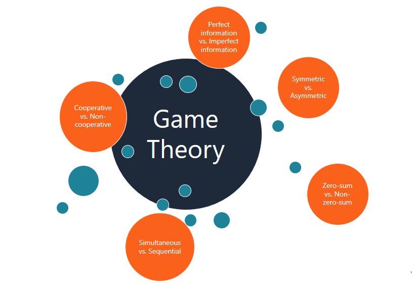
博弈论包含几个不同的主题,列举如下:

合作游戏cooperative game代写代考

合作博弈是通过确定任意 N 个子集 S 中的值(隶属度)来实现的。 在数学上,这种博弈也被称为隶属度函数。 合作博弈由一组玩家 $\mathrm{N}$ 和一对特征函数 $v$(N, v)$ 表示。 特征函数通常用于表示和分析合作博弈,有时也被称为博弈。
函数 $v$ 被解释为将奖励映射到 $N$ 中的每个联盟。 对于一个合伙关系 $\mathrm{~S}$ 来说,特征函数 $v(\mathrm{~S})$ 的值代表了 S 个玩家所能得到的最佳值,$v(S)$ 被称为合伙关系值。 通常假定 $v(\emptyset)=0$(无人参与的合伙关系无奖励)。
相对于合伙博弈中的奖励,还有一种方法可以描述成本函数 $C:2^N \rightarrow \mathbb{R}$,它映射了 N 中每个合伙关系的成本,这就是成本博弈(成本函数)$C:2^N \rightarrow \mathbb{R}$。 这就是成本博弈。 成本函数求出的值表示合伙关系中各参与方付出的成本。 合伙博弈中的概念很容易用成本博弈来重写。

非合作博弈noncooperative game代写代考

例如,在重复博弈中,即使没有这种制度框架,也可能会出现隐性合作,但这种博弈也包括在非合作博弈中。
此外,还有两个或两个以上参与者同时决定策略的战略博弈,以及两个或两个以上参与者轮流决定策略的发展博弈。 在发展型游戏中,参与者达成的协议和承诺也包括在非合作型游戏中。 因此,合作行为也可以受制于非合作博弈。
在非合作博弈中,每个博弈方都会独立制定策略。 非合作博弈的解法有两种含义:一种是 “规范含义”,即指导博弈者应如何行动;另一种是 “描述含义”,即显示博弈者的实际行为。
非合作博弈中一个重要的均衡概念是纳什均衡。

正则表达式博弈normal form game代写代考

与部署博弈一样,标准形式博弈是非合作博弈的基本表示形式,由三个要素组成:玩家集、策略空间和收益函数。 扩展博弈比标准形式博弈包含更多的信息,所有扩展博弈都可以转换成标准形式博弈。 另一方面,标准型博弈可以被视为同时移动博弈。 当棋手集和策略空间都是有限集时,已知在混合策略范围内存在纳什均衡和完全均衡(纳什定理)。
标准形式博弈也叫常规形式博弈或策略形式博弈。

其他相关科目课程代写:

  • Extensive-form game广式游戏
  • game of characteristic function form特征函数形式博弈

博弈论Game theory历史相关

安托万-奥古斯丁-库尔诺(Antoine Augustin Cournot)1838 年发表在他的《财富理论的数学原理研究》(Recherches sur les principes mathématiques de la théorie des richesses)一书中对双人博弈的分析,可以看作是纳什均衡概念在特定背景下的首次表述。

在 1938 年出版的著作《哈萨德游戏的应用》中,埃米尔-伯勒尔提出了双人零和博弈的最小值定理,即一方赢另一方输的博弈。

约翰-冯-诺依曼
1944 年,约翰-冯-诺依曼(John von Neumann)和奥斯卡-摩根斯特恩(Oskar Morgenstern)出版了《博弈与经济行为理论》(Theory of Games and Economic Behavior)一书,博弈论由此成为一个独立的研究领域。这部开创性著作详细介绍了解决零和博弈的方法。

1950 年左右,约翰-福布斯-纳什正式提出了均衡的一般概念,即后来的纳什均衡。这一概念概括了库诺的研究成果2,特别是加入了随机化策略的可能性。

统计代写请认准statistics-lab™. statistics-lab™为您的留学生涯保驾护航。

博弈论Game theory的相关课后作业范例

这是一篇关于博弈论Game theory的作业

问题 1.

Every finite strategic-form game has a mixedstrategy equilibrium.

Remark Remember that a pure-strategy equilibrium is an equilibrium in degenerate mixed strategies. The theorem does not assert the existence of an equilibrium with nondegenerate mixing.

Proof Since this is the archetypal existence proof in game theory, we will go through it in detail. The idea of the proof is to apply Kakutani’s fixed-point theorem to the players’ “reaction correspondences.” Player $i$ ‘s reaction correspondence, $r_i$, maps each strategy profilc $\sigma$ to the set of mixed strategies that maximize player $i$ ‘s payoff when his opponents play $\sigma_i$. (Although $r_i$ depends only on $\sigma_{-i}$ and not on $\sigma_i$, we write it as a function of the strategies of all players. because later we will look for a fixed point in the space $\Sigma$ of strategy profiles.) This is the natural generalization of the Cournot reaction function we defined above. Define the correspondence $r: \Sigma \rightrightarrows \Sigma$ to be the Cartesian product of the $r_i$. A fixed point of $r$ is a $\sigma$ such that $\sigma \in r(\sigma)$, so that, for each player, $\sigma_i \in r_i(\sigma)$. Thus, a fixed point of $r$ is a Nash equilibrium.

From Kakutani’s theorem, the following are sufficient conditions for $r: \Sigma \rightrightarrows \Sigma$ to have a fixed point:
(1) $\Sigma$ is a compact, ${ }^{17}$ convex,${ }^{18}$ nonempty subset of a (finite-dimensional) Fuclidean space.
(2) $r(\sigma)$ is nonempty for all $\sigma$.
(3) $r(\sigma)$ is convex for all $\sigma$.

(4) $r(\cdot)$ has a closed graph: If $\left(\sigma^n, \hat{\sigma}^n\right) \rightarrow(\sigma, \hat{\sigma})$ with $\hat{\sigma}^n \in r\left(\sigma^n\right)$, then $\hat{\sigma} \in r(\sigma)$. (This property is also often referred to as upper hemi-continuity. ${ }^{19}$ )
Let us check that these conditions are satisfied.
Condition 1 is easy – each $\Sigma_i$ is a simplex of dimension $\left(# S_i-1\right)$. Each player’s payoff function is linear, and therefore continuous in his own mixed strategy, and since continuous functions on compact sets attain maxima, condition 2 is satisfied. If $r(\sigma)$ were not convex, there would be a $\sigma^{\prime} \in r(\sigma)$, a $\sigma^{\prime \prime} \in r(\sigma)$, and a $\lambda \in(0,1)$ such that $\lambda \sigma^{\prime}+(1-\lambda) \sigma^{\prime \prime} \notin r(\sigma)$. But for each player $i$,
$$
u_i\left(j \sigma_i^{\prime}+(1-i) \sigma_i^{\prime \prime}, \sigma_{-i}\right)=\lambda u_i\left(\sigma_i^{\prime}, \sigma_{-i}\right)+(1-\lambda) u_i\left(\sigma_i^{\prime \prime}, \sigma_{-i}\right),
$$
so that if both $\sigma_i^{\prime}$ and $\sigma_i^{\prime \prime}$ are best responses to $\sigma_{-i}$, then so is their weighted average. This verifics condition 3 .

Finally, assume that condition 4 is violated so there is a sequence $\left(\sigma^n, \hat{\sigma}^n\right) \rightarrow(\sigma, \hat{\sigma}), \hat{\sigma}^n \in r\left(\sigma^n\right)$, but $\hat{\sigma} \notin r(\sigma)$. Then $\hat{\sigma}i \notin r_i(\sigma)$ for some player $i$. Thus, there is an $z>0$ and a $\sigma_i^{\prime}$ such that $u_i\left(\sigma_i^{\prime}, \sigma{-i}\right)>u_i\left(\hat{\sigma}i, \sigma{-i}\right)+3 \varepsilon$. Since $u_i$ is continuous and $\left(\sigma^n, \hat{\sigma}^n\right) \rightarrow(\sigma, \hat{\sigma})$, for $n$ sufficiently large we have
$$
u_i\left(\sigma_i^{\prime}, \sigma_{-i}^n\right)>u_i\left(\sigma_i^{\prime}, \sigma_{-i}\right)-\varepsilon>u_i\left(\hat{\sigma}i, \sigma{-i}\right)+2 \varepsilon>u_i\left(\hat{\sigma}i^n, \sigma{-i}^n\right)+\varepsilon .
$$

最后的总结:

通过对博弈论Game theory各方面的介绍,想必您对这门课有了初步的认识。如果你仍然不确定或对这方面感到困难,你仍然可以依靠我们的代写和辅导服务。我们拥有各个领域、具有丰富经验的专家。他们将保证你的 essay、assignment或者作业都完全符合要求、100%原创、无抄袭、并一定能获得高分。需要如何学术帮助的话,随时联系我们的客服。

R语言代写问卷设计与分析代写
PYTHON代写回归分析与线性模型代写
MATLAB代写方差分析与试验设计代写
STATA代写机器学习/统计学习代写
SPSS代写计量经济学代写
EVIEWS代写时间序列分析代写
EXCEL代写深度学习代写
SQL代写各种数据建模与可视化代写

统计代写|时间序列分析代写Time-Series Analysis代考|S-650

如果你也在 怎样代写时间序列Time Series 这个学科遇到相关的难题,请随时右上角联系我们的24/7代写客服。时间序列Time Series是在一段时间内以连续顺序出现的数据点序列。这可以与横截面数据进行对比,后者捕获一个时间点。在投资中,时间序列跟踪所选数据点(如证券价格)在指定时间段内的运动,并以固定的间隔记录数据点。没有必须包括的最小或最大时间,允许以一种方式收集数据,提供投资者或分析人员检查活动所寻求的信息。

时间序列Time Series可以取任何随时间变化的变量。在投资中,通常使用时间序列来跟踪一段时间内证券的价格。这可以在短期内跟踪,例如在一个工作日内某一小时的证券价格,或在长期内跟踪,例如在五年内每个月最后一天收盘的证券价格。

statistics-lab™ 为您的留学生涯保驾护航 在代写时间序列分析Time-Series Analysis方面已经树立了自己的口碑, 保证靠谱, 高质且原创的统计Statistics代写服务。我们的专家在代写时间序列分析Time-Series Analysis代写方面经验极为丰富,各种代写时间序列分析Time-Series Analysis相关的作业也就用不着说。

统计代写|时间序列分析代写Time-Series Analysis代考|S-650

统计代写|时间序列分析代写Time-Series Analysis代考|The Autocorrelation Function

The trouble with covariances is that they generally depend on the units with which $Y_t$ is measured. We can easily get around this problem by working correlations, which are just scaled versions of covariances. We have:
Definition 31 The correlation between $Y_t$ and $Y_{t-k}$ is:
$$
\operatorname{Corr}\left[Y_t, Y_{t-k}\right]=\frac{\operatorname{Cov}\left[Y_t, Y_{t-k}\right]}{\operatorname{Var}\left[Y_t\right]^{\frac{1}{2}} \operatorname{Var}\left[Y_{t-k}\right]^{\frac{1}{2}}} .
$$
Using stationarity we can simplify this considerably. Since
$$
\operatorname{Cov}\left[Y_t, Y_{t-k}\right]=\gamma(k)
$$
and by stationarity
$$
\operatorname{Var}\left[Y_t\right]^{\frac{1}{2}}=\operatorname{Var}\left[Y_{t-k}\right]^{\frac{1}{2}}=\gamma(0)^{\frac{1}{2}}
$$
we have:
$$
\operatorname{Corr}\left[Y_t, Y_{t-k}\right]=\frac{\gamma(k)}{\gamma(0)}
$$
With this in mind we can define the autocorrelation function
$$
\rho(k)=\operatorname{Corr}\left[Y_t, Y_{t-k}\right]
$$
as follows:
Definition 32 Autocorrelation Function: The autocorrelation function $\rho(k)$ is defined as:
$$
\rho(k)=\frac{\gamma(k)}{\gamma(0)}
$$

统计代写|时间序列分析代写Time-Series Analysis代考|The Autocorrelation Function of an AR(1) Process

We have :
Theorem 39 The autocorrelation function of a stationary AR(1) process is:
$$
\rho(k)=\phi^{|k|} .
$$
Proof. From Theorem 30 it follows that
$$
\begin{aligned}
\rho(k) & =\frac{\gamma(k)}{\gamma(0)} \
& =\frac{\phi^{|k|} \frac{\sigma^2}{1-\phi^2}}{\frac{\sigma^2}{1-\phi^2}} \
& =\phi^{|k|} .
\end{aligned}
$$

We plot $\rho(k)$ an $\operatorname{AR}(1)$ with $\phi=0.7$ below: ${ }^2$
$$
\rho(k) \text { when } \phi=0.7
$$
Since $|\phi|<1$ it follows that the autocorrelation function, like the autocovariance function, has the short-memory property so that $\rho(k)=O\left(\tau^k\right)$ as given in Section 2.2 with $A=1$ and $\tau=|\phi|$.

统计代写|时间序列分析代写Time-Series Analysis代考|S-650

时间序列分析代考

统计代写|时间序列分析代写Time-Series Analysis代考|The Autocorrelation Function

协方差的问题在于它们通常依赖于测量$Y_t$的单位。我们可以很容易地通过工作相关来解决这个问题,它只是协方差的缩放版本。我们有:
定义31 $Y_t$与$Y_{t-k}$的相关性为:
$$
\operatorname{Corr}\left[Y_t, Y_{t-k}\right]=\frac{\operatorname{Cov}\left[Y_t, Y_{t-k}\right]}{\operatorname{Var}\left[Y_t\right]^{\frac{1}{2}} \operatorname{Var}\left[Y_{t-k}\right]^{\frac{1}{2}}} .
$$
使用平稳性我们可以大大简化它。自从
$$
\operatorname{Cov}\left[Y_t, Y_{t-k}\right]=\gamma(k)
$$
通过平稳性
$$
\operatorname{Var}\left[Y_t\right]^{\frac{1}{2}}=\operatorname{Var}\left[Y_{t-k}\right]^{\frac{1}{2}}=\gamma(0)^{\frac{1}{2}}
$$
我们有:
$$
\operatorname{Corr}\left[Y_t, Y_{t-k}\right]=\frac{\gamma(k)}{\gamma(0)}
$$
考虑到这一点,我们可以定义自相关函数
$$
\rho(k)=\operatorname{Corr}\left[Y_t, Y_{t-k}\right]
$$
具体如下:
定义32自相关函数:自相关函数$\rho(k)$定义为:
$$
\rho(k)=\frac{\gamma(k)}{\gamma(0)}
$$

统计代写|时间序列分析代写Time-Series Analysis代考|The Autocorrelation Function of an AR(1) Process

我们有:
平稳AR(1)过程的自相关函数为:
$$
\rho(k)=\phi^{|k|} .
$$
证明。从定理30可以得出
$$
\begin{aligned}
\rho(k) & =\frac{\gamma(k)}{\gamma(0)} \
& =\frac{\phi^{|k|} \frac{\sigma^2}{1-\phi^2}}{\frac{\sigma^2}{1-\phi^2}} \
& =\phi^{|k|} .
\end{aligned}
$$

我们在下面用$\phi=0.7$绘制$\rho(k)$和$\operatorname{AR}(1)$: ${ }^2$
$$
\rho(k) \text { when } \phi=0.7
$$
由于$|\phi|<1$,因此自相关函数,像自协方差函数一样,具有短记忆特性,因此,$\rho(k)=O\left(\tau^k\right)$如2.2节中给出的$A=1$和$\tau=|\phi|$。

统计代写|时间序列分析代写Time-Series Analysis代考 请认准statistics-lab™

统计代写请认准statistics-lab™. statistics-lab™为您的留学生涯保驾护航。

金融工程代写

金融工程是使用数学技术来解决金融问题。金融工程使用计算机科学、统计学、经济学和应用数学领域的工具和知识来解决当前的金融问题,以及设计新的和创新的金融产品。

非参数统计代写

非参数统计指的是一种统计方法,其中不假设数据来自于由少数参数决定的规定模型;这种模型的例子包括正态分布模型和线性回归模型。

广义线性模型代考

广义线性模型(GLM)归属统计学领域,是一种应用灵活的线性回归模型。该模型允许因变量的偏差分布有除了正态分布之外的其它分布。

术语 广义线性模型(GLM)通常是指给定连续和/或分类预测因素的连续响应变量的常规线性回归模型。它包括多元线性回归,以及方差分析和方差分析(仅含固定效应)。

有限元方法代写

有限元方法(FEM)是一种流行的方法,用于数值解决工程和数学建模中出现的微分方程。典型的问题领域包括结构分析、传热、流体流动、质量运输和电磁势等传统领域。

有限元是一种通用的数值方法,用于解决两个或三个空间变量的偏微分方程(即一些边界值问题)。为了解决一个问题,有限元将一个大系统细分为更小、更简单的部分,称为有限元。这是通过在空间维度上的特定空间离散化来实现的,它是通过构建对象的网格来实现的:用于求解的数值域,它有有限数量的点。边界值问题的有限元方法表述最终导致一个代数方程组。该方法在域上对未知函数进行逼近。[1] 然后将模拟这些有限元的简单方程组合成一个更大的方程系统,以模拟整个问题。然后,有限元通过变化微积分使相关的误差函数最小化来逼近一个解决方案。

tatistics-lab作为专业的留学生服务机构,多年来已为美国、英国、加拿大、澳洲等留学热门地的学生提供专业的学术服务,包括但不限于Essay代写,Assignment代写,Dissertation代写,Report代写,小组作业代写,Proposal代写,Paper代写,Presentation代写,计算机作业代写,论文修改和润色,网课代做,exam代考等等。写作范围涵盖高中,本科,研究生等海外留学全阶段,辐射金融,经济学,会计学,审计学,管理学等全球99%专业科目。写作团队既有专业英语母语作者,也有海外名校硕博留学生,每位写作老师都拥有过硬的语言能力,专业的学科背景和学术写作经验。我们承诺100%原创,100%专业,100%准时,100%满意。

随机分析代写


随机微积分是数学的一个分支,对随机过程进行操作。它允许为随机过程的积分定义一个关于随机过程的一致的积分理论。这个领域是由日本数学家伊藤清在第二次世界大战期间创建并开始的。

时间序列分析代写

随机过程,是依赖于参数的一组随机变量的全体,参数通常是时间。 随机变量是随机现象的数量表现,其时间序列是一组按照时间发生先后顺序进行排列的数据点序列。通常一组时间序列的时间间隔为一恒定值(如1秒,5分钟,12小时,7天,1年),因此时间序列可以作为离散时间数据进行分析处理。研究时间序列数据的意义在于现实中,往往需要研究某个事物其随时间发展变化的规律。这就需要通过研究该事物过去发展的历史记录,以得到其自身发展的规律。

回归分析代写

多元回归分析渐进(Multiple Regression Analysis Asymptotics)属于计量经济学领域,主要是一种数学上的统计分析方法,可以分析复杂情况下各影响因素的数学关系,在自然科学、社会和经济学等多个领域内应用广泛。

MATLAB代写

MATLAB 是一种用于技术计算的高性能语言。它将计算、可视化和编程集成在一个易于使用的环境中,其中问题和解决方案以熟悉的数学符号表示。典型用途包括:数学和计算算法开发建模、仿真和原型制作数据分析、探索和可视化科学和工程图形应用程序开发,包括图形用户界面构建MATLAB 是一个交互式系统,其基本数据元素是一个不需要维度的数组。这使您可以解决许多技术计算问题,尤其是那些具有矩阵和向量公式的问题,而只需用 C 或 Fortran 等标量非交互式语言编写程序所需的时间的一小部分。MATLAB 名称代表矩阵实验室。MATLAB 最初的编写目的是提供对由 LINPACK 和 EISPACK 项目开发的矩阵软件的轻松访问,这两个项目共同代表了矩阵计算软件的最新技术。MATLAB 经过多年的发展,得到了许多用户的投入。在大学环境中,它是数学、工程和科学入门和高级课程的标准教学工具。在工业领域,MATLAB 是高效研究、开发和分析的首选工具。MATLAB 具有一系列称为工具箱的特定于应用程序的解决方案。对于大多数 MATLAB 用户来说非常重要,工具箱允许您学习应用专业技术。工具箱是 MATLAB 函数(M 文件)的综合集合,可扩展 MATLAB 环境以解决特定类别的问题。可用工具箱的领域包括信号处理、控制系统、神经网络、模糊逻辑、小波、仿真等。

R语言代写问卷设计与分析代写
PYTHON代写回归分析与线性模型代写
MATLAB代写方差分析与试验设计代写
STATA代写机器学习/统计学习代写
SPSS代写计量经济学代写
EVIEWS代写时间序列分析代写
EXCEL代写深度学习代写
SQL代写各种数据建模与可视化代写

统计代写|时间序列分析代写Time-Series Analysis代考|STK9060

如果你也在 怎样代写时间序列Time Series 这个学科遇到相关的难题,请随时右上角联系我们的24/7代写客服。时间序列Time Series是在一段时间内以连续顺序出现的数据点序列。这可以与横截面数据进行对比,后者捕获一个时间点。在投资中,时间序列跟踪所选数据点(如证券价格)在指定时间段内的运动,并以固定的间隔记录数据点。没有必须包括的最小或最大时间,允许以一种方式收集数据,提供投资者或分析人员检查活动所寻求的信息。

时间序列Time Series可以取任何随时间变化的变量。在投资中,通常使用时间序列来跟踪一段时间内证券的价格。这可以在短期内跟踪,例如在一个工作日内某一小时的证券价格,或在长期内跟踪,例如在五年内每个月最后一天收盘的证券价格。

statistics-lab™ 为您的留学生涯保驾护航 在代写时间序列分析Time-Series Analysis方面已经树立了自己的口碑, 保证靠谱, 高质且原创的统计Statistics代写服务。我们的专家在代写时间序列分析Time-Series Analysis代写方面经验极为丰富,各种代写时间序列分析Time-Series Analysis相关的作业也就用不着说。

统计代写|时间序列分析代写Time-Series Analysis代考|STK9060

统计代写|时间序列分析代写Time-Series Analysis代考|The Autocovariance Function

An important implication of stationarity is that the covariance between the business cycle in say the first and third quarters of say 1999 is the same as the covariance between the business cycle the first and third quarters of say 1963 . In general covariances only depend on the number of periods separating $Y_t$ and $Y_s$ so that:

Theorem 20 If $Y_t$ is stationary then $\operatorname{Cov}\left[Y_{t_1}, Y_{t_2}\right]$ depends only on $k=t_1-t_2$; that is the number of periods separating $t_1$ and $t_2$.

Since we will often be focusing on covariances, and since $\operatorname{Cov}\left[Y_t, Y_{t-k}\right]$ only depends on $k$, let us define this as a function of $k$ as: $\gamma(k)$, which we will refer to as the autocovariance function so that:

Definition 21 Autocovariance Function: Let $Y_t$ be a stationary time series with $E\left[Y_t\right]=0$. The autocovariance function for $Y_t$, denoted as $\gamma(k)$, is defined for $k=0, \pm 1, \pm 2, \pm 3, \ldots \pm \infty$ as:
$$
\gamma(k) \equiv E\left[Y_t Y_{t-k}\right]=\operatorname{Cov}\left[Y_t, Y_{t-k}\right] .
$$
We have the following results for the autocovariance function:
Theorem $22 \gamma(0)=\operatorname{Var}\left[Y_t\right]>0$
Theorem $23 \gamma(k)=E\left[Y_t Y_{t-k}\right]=E\left[Y_s Y_{s-k}\right]$ for any $t$ and $s$.
Theorem $24 \gamma(-k)=\gamma(k)(\gamma(k)$ is an even function $)$

统计代写|时间序列分析代写Time-Series Analysis代考|The AR(1) Model

For the AR(1) model we have already shown that:
$$
\gamma(0)=\operatorname{Var}\left[Y_t\right]=\frac{\sigma^2}{1-\phi^2}
$$
and that for $k>0$ :
$$
\begin{aligned}
\gamma(k) & =\phi^k \gamma(0) \
& =\phi^k \frac{\sigma^2}{1-\phi^2} .
\end{aligned}
$$
We can make this formula correct for all $k$ by appealing to Theorem 24 and replacing $k$ with $|k|$ to obtain:

Theorem 30 For an $A R(1)$ process the autocovariance function is given by:
$$
\gamma(k)=\frac{\phi^{|k|} \sigma^2}{1-\phi^2} .
$$

统计代写|时间序列分析代写Time-Series Analysis代考|STK9060

时间序列分析代考

统计代写|时间序列分析代写Time-Series Analysis代考|The Autocovariance Function

平稳性的一个重要含义是1999年第一季度和第三季度商业周期之间的协方差与1963年第一季度和第三季度商业周期之间的协方差是相同的。一般来说,协方差只取决于$Y_t$和$Y_s$之间的周期数,因此:

定理20如果$Y_t$是平稳的,那么$\operatorname{Cov}\left[Y_{t_1}, Y_{t_2}\right]$只依赖于$k=t_1-t_2$;这是分隔$t_1$和$t_2$的周期数。

由于我们将经常关注协方差,并且由于$\operatorname{Cov}\left[Y_t, Y_{t-k}\right]$只依赖于$k$,让我们将其定义为$k$的函数:$\gamma(k)$,我们将其称为自协方差函数,以便:

定义21自协方差函数:设$Y_t$为平稳时间序列,$E\left[Y_t\right]=0$。将$Y_t$的自协方差函数记为$\gamma(k)$,将$k=0, \pm 1, \pm 2, \pm 3, \ldots \pm \infty$定义为:
$$
\gamma(k) \equiv E\left[Y_t Y_{t-k}\right]=\operatorname{Cov}\left[Y_t, Y_{t-k}\right] .
$$
对于自协方差函数,我们得到如下结果:
定理$22 \gamma(0)=\operatorname{Var}\left[Y_t\right]>0$
定理$23 \gamma(k)=E\left[Y_t Y_{t-k}\right]=E\left[Y_s Y_{s-k}\right]$适用于任何$t$和$s$。
定理$24 \gamma(-k)=\gamma(k)(\gamma(k)$是偶函数 $)$

统计代写|时间序列分析代写Time-Series Analysis代考|The AR(1) Model

对于AR(1)模型,我们已经表明:
$$
\gamma(0)=\operatorname{Var}\left[Y_t\right]=\frac{\sigma^2}{1-\phi^2}
$$
对于$k>0$:
$$
\begin{aligned}
\gamma(k) & =\phi^k \gamma(0) \
& =\phi^k \frac{\sigma^2}{1-\phi^2} .
\end{aligned}
$$
我们可以利用定理24,将$k$替换为$|k|$,从而使这个公式适用于所有$k$:

定理30对于$A R(1)$过程,自协方差函数为:
$$
\gamma(k)=\frac{\phi^{|k|} \sigma^2}{1-\phi^2} .
$$

统计代写|时间序列分析代写Time-Series Analysis代考 请认准statistics-lab™

统计代写请认准statistics-lab™. statistics-lab™为您的留学生涯保驾护航。

金融工程代写

金融工程是使用数学技术来解决金融问题。金融工程使用计算机科学、统计学、经济学和应用数学领域的工具和知识来解决当前的金融问题,以及设计新的和创新的金融产品。

非参数统计代写

非参数统计指的是一种统计方法,其中不假设数据来自于由少数参数决定的规定模型;这种模型的例子包括正态分布模型和线性回归模型。

广义线性模型代考

广义线性模型(GLM)归属统计学领域,是一种应用灵活的线性回归模型。该模型允许因变量的偏差分布有除了正态分布之外的其它分布。

术语 广义线性模型(GLM)通常是指给定连续和/或分类预测因素的连续响应变量的常规线性回归模型。它包括多元线性回归,以及方差分析和方差分析(仅含固定效应)。

有限元方法代写

有限元方法(FEM)是一种流行的方法,用于数值解决工程和数学建模中出现的微分方程。典型的问题领域包括结构分析、传热、流体流动、质量运输和电磁势等传统领域。

有限元是一种通用的数值方法,用于解决两个或三个空间变量的偏微分方程(即一些边界值问题)。为了解决一个问题,有限元将一个大系统细分为更小、更简单的部分,称为有限元。这是通过在空间维度上的特定空间离散化来实现的,它是通过构建对象的网格来实现的:用于求解的数值域,它有有限数量的点。边界值问题的有限元方法表述最终导致一个代数方程组。该方法在域上对未知函数进行逼近。[1] 然后将模拟这些有限元的简单方程组合成一个更大的方程系统,以模拟整个问题。然后,有限元通过变化微积分使相关的误差函数最小化来逼近一个解决方案。

tatistics-lab作为专业的留学生服务机构,多年来已为美国、英国、加拿大、澳洲等留学热门地的学生提供专业的学术服务,包括但不限于Essay代写,Assignment代写,Dissertation代写,Report代写,小组作业代写,Proposal代写,Paper代写,Presentation代写,计算机作业代写,论文修改和润色,网课代做,exam代考等等。写作范围涵盖高中,本科,研究生等海外留学全阶段,辐射金融,经济学,会计学,审计学,管理学等全球99%专业科目。写作团队既有专业英语母语作者,也有海外名校硕博留学生,每位写作老师都拥有过硬的语言能力,专业的学科背景和学术写作经验。我们承诺100%原创,100%专业,100%准时,100%满意。

随机分析代写


随机微积分是数学的一个分支,对随机过程进行操作。它允许为随机过程的积分定义一个关于随机过程的一致的积分理论。这个领域是由日本数学家伊藤清在第二次世界大战期间创建并开始的。

时间序列分析代写

随机过程,是依赖于参数的一组随机变量的全体,参数通常是时间。 随机变量是随机现象的数量表现,其时间序列是一组按照时间发生先后顺序进行排列的数据点序列。通常一组时间序列的时间间隔为一恒定值(如1秒,5分钟,12小时,7天,1年),因此时间序列可以作为离散时间数据进行分析处理。研究时间序列数据的意义在于现实中,往往需要研究某个事物其随时间发展变化的规律。这就需要通过研究该事物过去发展的历史记录,以得到其自身发展的规律。

回归分析代写

多元回归分析渐进(Multiple Regression Analysis Asymptotics)属于计量经济学领域,主要是一种数学上的统计分析方法,可以分析复杂情况下各影响因素的数学关系,在自然科学、社会和经济学等多个领域内应用广泛。

MATLAB代写

MATLAB 是一种用于技术计算的高性能语言。它将计算、可视化和编程集成在一个易于使用的环境中,其中问题和解决方案以熟悉的数学符号表示。典型用途包括:数学和计算算法开发建模、仿真和原型制作数据分析、探索和可视化科学和工程图形应用程序开发,包括图形用户界面构建MATLAB 是一个交互式系统,其基本数据元素是一个不需要维度的数组。这使您可以解决许多技术计算问题,尤其是那些具有矩阵和向量公式的问题,而只需用 C 或 Fortran 等标量非交互式语言编写程序所需的时间的一小部分。MATLAB 名称代表矩阵实验室。MATLAB 最初的编写目的是提供对由 LINPACK 和 EISPACK 项目开发的矩阵软件的轻松访问,这两个项目共同代表了矩阵计算软件的最新技术。MATLAB 经过多年的发展,得到了许多用户的投入。在大学环境中,它是数学、工程和科学入门和高级课程的标准教学工具。在工业领域,MATLAB 是高效研究、开发和分析的首选工具。MATLAB 具有一系列称为工具箱的特定于应用程序的解决方案。对于大多数 MATLAB 用户来说非常重要,工具箱允许您学习应用专业技术。工具箱是 MATLAB 函数(M 文件)的综合集合,可扩展 MATLAB 环境以解决特定类别的问题。可用工具箱的领域包括信号处理、控制系统、神经网络、模糊逻辑、小波、仿真等。

R语言代写问卷设计与分析代写
PYTHON代写回归分析与线性模型代写
MATLAB代写方差分析与试验设计代写
STATA代写机器学习/统计学习代写
SPSS代写计量经济学代写
EVIEWS代写时间序列分析代写
EXCEL代写深度学习代写
SQL代写各种数据建模与可视化代写

统计代写|时间序列分析代写Time-Series Analysis代考|MGSC575

如果你也在 怎样代写时间序列Time Series 这个学科遇到相关的难题,请随时右上角联系我们的24/7代写客服。时间序列Time Series是在一段时间内以连续顺序出现的数据点序列。这可以与横截面数据进行对比,后者捕获一个时间点。在投资中,时间序列跟踪所选数据点(如证券价格)在指定时间段内的运动,并以固定的间隔记录数据点。没有必须包括的最小或最大时间,允许以一种方式收集数据,提供投资者或分析人员检查活动所寻求的信息。

时间序列Time Series可以取任何随时间变化的变量。在投资中,通常使用时间序列来跟踪一段时间内证券的价格。这可以在短期内跟踪,例如在一个工作日内某一小时的证券价格,或在长期内跟踪,例如在五年内每个月最后一天收盘的证券价格。

statistics-lab™ 为您的留学生涯保驾护航 在代写时间序列分析Time-Series Analysis方面已经树立了自己的口碑, 保证靠谱, 高质且原创的统计Statistics代写服务。我们的专家在代写时间序列分析Time-Series Analysis代写方面经验极为丰富,各种代写时间序列分析Time-Series Analysis相关的作业也就用不着说。

统计代写|时间序列分析代写Time-Series Analysis代考|MGSC575

统计代写|时间序列分析代写Time-Series Analysis代考|The Short-Memory Property

Many of the models that we will be considering will have the property that they quickly forget or quickly become independent of what occurs either in the distant future or the distant past. This forgetting occurs at an exponential rate which represents a very rapid type of decay.

For example if you have a pie in the fridge and you eat one-half of the pie each day, you will quickly have almost no pie. After only ten days you would have:
$$
\left(\frac{1}{2}\right)^{10}=\frac{1}{1024}
$$
or about one-thousandth of a pie; maybe a couple of crumbs.
We will see that for stationary $\operatorname{ARMA}(\mathrm{p}, \mathrm{q})$ processes, the infinite moving average weights: $\psi_k$, the autocorrelation function $\rho(k)$ and the forecast function $E_t\left[Y_{t+k}\right]$, all functions of the number of periods $k$, all have the short-memory property which we now define:

Definition 12 Short-Memory: Let $P_k$ for $k=0,1,2, \ldots \infty$ be some numerical property of a stationary time series which depends on $k$, the number of periods. We say $P_k$ displays a short-memory or $P_k=O\left(\tau^k\right)$ if
$$
\left|P_k\right| \leq A \tau^k
$$
where $A \geq 0$ and $0<\tau<1$.

If $P_k=O\left(\tau^k\right)$ or if $P_k$ has a short-memory then $P_k$ decays rapidly in the same, manner that is at least as fast as $\tau^k$ decays to zero as $k \rightarrow \infty$. For example if:
$$
P_k=10 \cos (2 k)\left(-\frac{1}{2}\right)^k
$$
then $P_k$ decays rapidly in a manner which is bounded by exponential decay since $|\cos (2 k)| \leq 1$ and so we have:
$$
\left|P_k\right| \leq 10\left(\frac{1}{2}\right)^k=A \tau^k
$$
where $\tau=\frac{1}{2}$ and $A=10$. This is illustrated in the plot below:
$$
P_k=10 \cos (2 k)\left(-\frac{1}{2}\right)^k
$$
Not everything decays so rapidly. For example if we reverse the $\frac{1}{2}$ and the $k$ in $\left(\frac{1}{2}\right)^k$ we obtain:
$$
Q_k=\frac{1}{k^{\frac{1}{2}}}=k^{-\frac{1}{2}} .
$$

统计代写|时间序列分析代写Time-Series Analysis代考|The AR(1) Model

The simplest interesting model for $Y_t$ is a first-order autoregressive process or $\mathrm{AR}(1)$ which can be written as:
$$
Y_t=\phi Y_{t-1}+a_t, a_t \sim \text { i.i.n }\left(0, \sigma^2\right),
$$
where i.i.n. $\left(0, \sigma^2\right)$ means that $a_t$ is independently and identically distributed (i.i.d.) with a normal distribution with mean 0 and variance $\sigma^2$ so that the density of $a_t$ is:
$$
p\left(a_t\right)=\frac{1}{\sqrt{2 \pi \sigma^2}} e^{-\frac{1}{2} a_t^2} .
$$
We can attempt to calculate $E\left[Y_t\right]$ by taking expectations of both sides of (2.6) to obtain:
$$
\begin{aligned}
E\left[Y_t\right] & =\phi E\left[Y_{t-1}\right]+E\left[a_t\right] \
& =\phi E\left[Y_{t-1}\right]
\end{aligned}
$$
since $E\left[a_t\right]=0$. We now need to find $E\left[Y_{t-1}\right]$. We could try the same approach with $E\left[Y_{t-1}\right]$ since $Y_{t-1}=\phi Y_{t-2}+a_{t-1}$ from which we would conclude that: $E\left[Y_{t-1}\right]=\phi E\left[Y_{t-2}\right]$ so that:
$$
E\left[Y_t\right]=\phi^2 E\left[Y_{t-2}\right] ;
$$
but now we now need to find $E\left[Y_{t-2}\right]$. Clearly this process will never end.
If, however, we assume stationarity then it is possible to break this infinite regress since by the definition of stationarity in Definition 7:
$$
E\left[Y_t\right]=E\left[Y_{t-1}\right] .
$$
It then follows from (2.8) that:
$$
E\left[Y_t\right]=\phi E\left[Y_t\right]
$$
or
$$
(1-\phi) E\left[Y_t\right]=0 .
$$

统计代写|时间序列分析代写Time-Series Analysis代考|MGSC575

时间序列分析代考

统计代写|时间序列分析代写Time-Series Analysis代考|The Short-Memory Property

我们将要考虑的许多模型都具有这样的特性,即它们很快就会忘记或很快就会独立于遥远的将来或遥远的过去发生的事情。这种遗忘以指数速度发生,这代表了一种非常快速的衰退。

例如,如果你在冰箱里有一个派,你每天吃一半的派,你很快就没有派了。仅仅十天之后,你就会:
$$
\left(\frac{1}{2}\right)^{10}=\frac{1}{1024}
$$
或者是馅饼的千分之一;可能会有一些面包屑。
我们将看到,对于平稳$\operatorname{ARMA}(\mathrm{p}, \mathrm{q})$过程,无限移动平均权重:$\psi_k$,自相关函数$\rho(k)$和预测函数$E_t\left[Y_{t+k}\right]$,所有周期数的函数$k$,都具有我们现在定义的短记忆属性:

定义12短时记忆:设$k=0,1,2, \ldots \infty$中的$P_k$是一个平稳时间序列的一些数值性质,它取决于$k$的周期数。我们说$P_k$显示短记忆或$P_k=O\left(\tau^k\right)$ if
$$
\left|P_k\right| \leq A \tau^k
$$
其中$A \geq 0$和$0<\tau<1$。

如果$P_k=O\left(\tau^k\right)$或$P_k$有短记忆,那么$P_k$以同样的方式快速衰减,至少与$\tau^k$衰减到零的速度一样快$k \rightarrow \infty$。例如:
$$
P_k=10 \cos (2 k)\left(-\frac{1}{2}\right)^k
$$
然后$P_k$以指数衰减的方式快速衰减,从$|\cos (2 k)| \leq 1$开始,所以我们有:
$$
\left|P_k\right| \leq 10\left(\frac{1}{2}\right)^k=A \tau^k
$$
其中$\tau=\frac{1}{2}$和$A=10$。下面的图表说明了这一点:
$$
P_k=10 \cos (2 k)\left(-\frac{1}{2}\right)^k
$$
并不是所有东西都衰得这么快。例如,如果我们将$\left(\frac{1}{2}\right)^k$中的$\frac{1}{2}$和$k$颠倒过来,我们得到:
$$
Q_k=\frac{1}{k^{\frac{1}{2}}}=k^{-\frac{1}{2}} .
$$

统计代写|时间序列分析代写Time-Series Analysis代考|The AR(1) Model

最简单有趣的$Y_t$模型是一阶自回归过程或$\mathrm{AR}(1)$,可以写成:
$$
Y_t=\phi Y_{t-1}+a_t, a_t \sim \text { i.i.n }\left(0, \sigma^2\right),
$$
式中I.I.N. $\left(0, \sigma^2\right)$表示$a_t$为独立同分布(i.i.d),为均值为0,方差为$\sigma^2$的正态分布,则$a_t$的密度为:
$$
p\left(a_t\right)=\frac{1}{\sqrt{2 \pi \sigma^2}} e^{-\frac{1}{2} a_t^2} .
$$
我们可以尝试通过对式(2.6)两边的期望值来计算$E\left[Y_t\right]$,得到:
$$
\begin{aligned}
E\left[Y_t\right] & =\phi E\left[Y_{t-1}\right]+E\left[a_t\right] \
& =\phi E\left[Y_{t-1}\right]
\end{aligned}
$$
自从$E\left[a_t\right]=0$。我们现在需要找到$E\left[Y_{t-1}\right]$。我们可以尝试同样的方法与$E\left[Y_{t-1}\right]$,因为$Y_{t-1}=\phi Y_{t-2}+a_{t-1}$,从中我们可以得出结论:$E\left[Y_{t-1}\right]=\phi E\left[Y_{t-2}\right]$,因此:
$$
E\left[Y_t\right]=\phi^2 E\left[Y_{t-2}\right] ;
$$
现在我们需要找到$E\left[Y_{t-2}\right]$。显然,这个过程永远不会结束。
然而,如果我们假设平稳性,那么就有可能打破这种无限回归,因为根据定义7中的平稳性定义:
$$
E\left[Y_t\right]=E\left[Y_{t-1}\right] .
$$
由式(2.8)可知:
$$
E\left[Y_t\right]=\phi E\left[Y_t\right]
$$

$$
(1-\phi) E\left[Y_t\right]=0 .
$$

统计代写|时间序列分析代写Time-Series Analysis代考 请认准statistics-lab™

统计代写请认准statistics-lab™. statistics-lab™为您的留学生涯保驾护航。

金融工程代写

金融工程是使用数学技术来解决金融问题。金融工程使用计算机科学、统计学、经济学和应用数学领域的工具和知识来解决当前的金融问题,以及设计新的和创新的金融产品。

非参数统计代写

非参数统计指的是一种统计方法,其中不假设数据来自于由少数参数决定的规定模型;这种模型的例子包括正态分布模型和线性回归模型。

广义线性模型代考

广义线性模型(GLM)归属统计学领域,是一种应用灵活的线性回归模型。该模型允许因变量的偏差分布有除了正态分布之外的其它分布。

术语 广义线性模型(GLM)通常是指给定连续和/或分类预测因素的连续响应变量的常规线性回归模型。它包括多元线性回归,以及方差分析和方差分析(仅含固定效应)。

有限元方法代写

有限元方法(FEM)是一种流行的方法,用于数值解决工程和数学建模中出现的微分方程。典型的问题领域包括结构分析、传热、流体流动、质量运输和电磁势等传统领域。

有限元是一种通用的数值方法,用于解决两个或三个空间变量的偏微分方程(即一些边界值问题)。为了解决一个问题,有限元将一个大系统细分为更小、更简单的部分,称为有限元。这是通过在空间维度上的特定空间离散化来实现的,它是通过构建对象的网格来实现的:用于求解的数值域,它有有限数量的点。边界值问题的有限元方法表述最终导致一个代数方程组。该方法在域上对未知函数进行逼近。[1] 然后将模拟这些有限元的简单方程组合成一个更大的方程系统,以模拟整个问题。然后,有限元通过变化微积分使相关的误差函数最小化来逼近一个解决方案。

tatistics-lab作为专业的留学生服务机构,多年来已为美国、英国、加拿大、澳洲等留学热门地的学生提供专业的学术服务,包括但不限于Essay代写,Assignment代写,Dissertation代写,Report代写,小组作业代写,Proposal代写,Paper代写,Presentation代写,计算机作业代写,论文修改和润色,网课代做,exam代考等等。写作范围涵盖高中,本科,研究生等海外留学全阶段,辐射金融,经济学,会计学,审计学,管理学等全球99%专业科目。写作团队既有专业英语母语作者,也有海外名校硕博留学生,每位写作老师都拥有过硬的语言能力,专业的学科背景和学术写作经验。我们承诺100%原创,100%专业,100%准时,100%满意。

随机分析代写


随机微积分是数学的一个分支,对随机过程进行操作。它允许为随机过程的积分定义一个关于随机过程的一致的积分理论。这个领域是由日本数学家伊藤清在第二次世界大战期间创建并开始的。

时间序列分析代写

随机过程,是依赖于参数的一组随机变量的全体,参数通常是时间。 随机变量是随机现象的数量表现,其时间序列是一组按照时间发生先后顺序进行排列的数据点序列。通常一组时间序列的时间间隔为一恒定值(如1秒,5分钟,12小时,7天,1年),因此时间序列可以作为离散时间数据进行分析处理。研究时间序列数据的意义在于现实中,往往需要研究某个事物其随时间发展变化的规律。这就需要通过研究该事物过去发展的历史记录,以得到其自身发展的规律。

回归分析代写

多元回归分析渐进(Multiple Regression Analysis Asymptotics)属于计量经济学领域,主要是一种数学上的统计分析方法,可以分析复杂情况下各影响因素的数学关系,在自然科学、社会和经济学等多个领域内应用广泛。

MATLAB代写

MATLAB 是一种用于技术计算的高性能语言。它将计算、可视化和编程集成在一个易于使用的环境中,其中问题和解决方案以熟悉的数学符号表示。典型用途包括:数学和计算算法开发建模、仿真和原型制作数据分析、探索和可视化科学和工程图形应用程序开发,包括图形用户界面构建MATLAB 是一个交互式系统,其基本数据元素是一个不需要维度的数组。这使您可以解决许多技术计算问题,尤其是那些具有矩阵和向量公式的问题,而只需用 C 或 Fortran 等标量非交互式语言编写程序所需的时间的一小部分。MATLAB 名称代表矩阵实验室。MATLAB 最初的编写目的是提供对由 LINPACK 和 EISPACK 项目开发的矩阵软件的轻松访问,这两个项目共同代表了矩阵计算软件的最新技术。MATLAB 经过多年的发展,得到了许多用户的投入。在大学环境中,它是数学、工程和科学入门和高级课程的标准教学工具。在工业领域,MATLAB 是高效研究、开发和分析的首选工具。MATLAB 具有一系列称为工具箱的特定于应用程序的解决方案。对于大多数 MATLAB 用户来说非常重要,工具箱允许您学习应用专业技术。工具箱是 MATLAB 函数(M 文件)的综合集合,可扩展 MATLAB 环境以解决特定类别的问题。可用工具箱的领域包括信号处理、控制系统、神经网络、模糊逻辑、小波、仿真等。

R语言代写问卷设计与分析代写
PYTHON代写回归分析与线性模型代写
MATLAB代写方差分析与试验设计代写
STATA代写机器学习/统计学习代写
SPSS代写计量经济学代写
EVIEWS代写时间序列分析代写
EXCEL代写深度学习代写
SQL代写各种数据建模与可视化代写

统计代写|随机过程代写stochastic process代考|IE2084

如果你也在 怎样代写随机过程Stochastic Porcesses 这个学科遇到相关的难题,请随时右上角联系我们的24/7代写客服。随机过程Stochastic Porcesses是指一个系统在特定的时间有观测值,结果,即每次的观测值是一个随机变量。

随机过程Stochastic Porcesses在是由一些数学集合索引的随机变量的集合。每个概率和随机过程都与集合中的一个元素唯一地相关联。索引集是用来索引随机变量的集合。索引集传统上是实数的子集,例如自然数,这为索引集提供了时间解释。

statistics-lab™ 为您的留学生涯保驾护航 在代写随机过程stochastic process方面已经树立了自己的口碑, 保证靠谱, 高质且原创的统计Statistics代写服务。我们的专家在代写随机过程stochastic process代写方面经验极为丰富,各种代写随机过程stochastic process相关的作业也就用不着说。

统计代写|随机过程代写stochastic process代考|STAT433

统计代写|随机过程代写stochastic process代考|Probability distribution

It may be seen that the probability distribution of $X_r, X_{r+1}, \ldots, X_{r+n}$ can be computed in terms of the transition probabilities $p_{j k}$ and the initial distribution of $X_r$. Suppose, for simplicity, that $r=0$, then
$$
\begin{aligned}
\operatorname{Pr}\left{X_0\right. & \left.=a, X_1=b, \ldots, X_{n-2}=i, X_{n-1}=j, X_n=k\right} \
& =\operatorname{Pr}\left{X_n=k \mid X_{n-1}=j, \cdots, X_0=a\right} \operatorname{Pr}\left{X_{n-1}=j, \cdots, X_0=a\right} \
& =\operatorname{Pr}\left{X_n=k \mid X_{n-1}=j\right} \operatorname{Pr}\left{X_{n-1}=j \mid X_{n-2}=i\right} \operatorname{Pr}\left{X_{n-2}=i, \cdots, X_0=a\right} \
& =\operatorname{Pr}\left{X_n=k \mid X_{n-1}=j\right} \operatorname{Pr}\left{X_{n-1}=j \mid X_{n-2}=i\right} \cdots \operatorname{Pr}\left{X_1=b \mid X_0=a\right} \operatorname{Pr}\left{X_0=a\right} \
& =\left{\operatorname{Pr}\left(X_0=a\right)\right} p_{a b} \cdots p_{i j} p_{j k} .
\end{aligned}
$$
Thus,
$$
\begin{aligned}
\operatorname{Pr}\left{X_r\right. & \left.=a, X_{r+1}=b, \ldots, X_{r+n-2}=i, X_{r+n-1}=j, X_{r+n}=k\right} \
& =\left{\operatorname{Pr}\left(X_r=a\right)\right} p_{a b} \ldots p_{i j} p_{j k} .
\end{aligned}
$$
Example 1(g). Let $\left{X_n, n \geq 0\right}$ be a Markov chain with three states $0,1,2$ and with transition matrix
$$
\left(\begin{array}{ccc}
3 / 4 & 1 / 4 & 0 \
1 / 4 & 1 / 2 & 1 / 4 \
0 & 3 / 4 & 1 / 4
\end{array}\right)
$$
and the initial distribution $\operatorname{Pr}\left{X_0=i\right}=\frac{1}{3}, i=0,1,2$.
We have
$$
\begin{aligned}
& \operatorname{Pr}\left{X_1=1 \mid X_0=2\right}=\frac{3}{4} \
& \operatorname{Pr}\left{X_2=2 \mid X_1=1\right}=\frac{1}{4} \
& \operatorname{Pr}\left{X_2=2, X_1=1 \mid X_0=2\right} \
& =\operatorname{Pr}\left{X_2=2 \mid X_1=1\right} \operatorname{Pr}\left{X_1=1 \mid X_0=2\right}=\frac{1}{4} \cdot \frac{3}{4}=\frac{3}{16}
\end{aligned}
$$

\begin{aligned}
\operatorname{Pr}\left{X_2\right. & \left.=2, X_1=1, X_0=2\right} \
& =\operatorname{Pr}\left{X_2=2, X_1=1 \mid X_0=2\right} \operatorname{Pr}\left{X_0=2\right}=\frac{3}{16} \cdot \frac{1}{3}=\frac{1}{16} \
\operatorname{Pr}\left{X_3\right. & \left.=1, X_2=2, X_1=1, X_0=2\right} \
& =\operatorname{Pr}\left{X_3=1 \mid X_2=2, X_1=1, X_0=2\right} \times \operatorname{Pr}\left{X_2=2, X_1=1, X_0=2\right} \
& =\operatorname{Pr}\left{X_3=1 \mid X_2=2\right}\left(\frac{1}{16}\right)=\frac{3}{4} \cdot \frac{1}{16}=\frac{3}{64} .
\end{aligned}

统计代写|随机过程代写stochastic process代考|Strong Markov property

Stopping time for a sequence of r.v.’s $\left{X_n\right}$ is a random variable (see Sec. 6.4.1).
Let $N$ be a stopping time for a Markov chain $\left{X_n, n>0\right}$ and let $A$ and $B$ to two events (relating to $X_n$ and happening) prior and posterior respectively to $N$. Then
$$
\operatorname{Pr}\left{B \mid X_N=i, A\right}=\operatorname{Pr}\left{B \mid X_N=i\right} .
$$
This is called the strong Markov property. It shows that if $N$ is a stopping time for a Markov chain $\left{X_n, n>0\right}$, then the evolution of the chain starts afresh from the state reached at time $N$.

Strong Markov property is implied by the Markov property; both the properties are equivalent when $N$ is constant (a degenerate r.v.).
Every discrete time Markov chain $\left{X_n, n \geq 0\right}$ possesses the strong Markov property.

Definition. A Markov chain $\left{X_n\right}$ is said to be of order $s(s=1,2,3, \ldots)$, if, for all $n$,
$$
\begin{aligned}
\operatorname{Pr}\left{X_n\right. & \left.=k \mid X_{n-1}=j, X_{n-2}=j_1, \ldots, X_{n-s}=j_{s-1}, \ldots\right} \
& =\operatorname{Pr}\left{X_n=k \mid X_{n-1}=j, \ldots, X_{n-s}=j_{s-1}\right} .
\end{aligned}
$$
whenever the 1.h.s. is defined.
A Markov chain $\left{X_n\right}$ is said to be of order one (or simply a Markov chain) if
$$
\begin{aligned}
\operatorname{Pr}\left{X_n\right. & \left.=k \mid X_{n-1}=j, X_{n-2}=j_1, \ldots\right}=\operatorname{Pr}\left{X_n=k \mid X_{n-1}=j\right} \
& =p_{j k} .
\end{aligned}
$$
whenever $\operatorname{Pr}\left{X_{n-1}=j, X_{n-2}=j_1, \ldots\right}>0$.
Unless explicitly stated otherwise, we shall mean by Markov chain, a chain of order one, to which we shall mostly confine ourselves here. A chain is said to be of order zero if $p_{j k}=p_k$ for all $j$. This implies independence of $X_n$ and $X_{n-1}$. For example, for the Bernoulli coin tossing experiment, the t.p.m. is $\left(\begin{array}{ll}q & p \ q & p\end{array}\right)=\left(\begin{array}{l}1 \ 1\end{array}\right)(q, p)=\mathbf{e}(q, p)$.
Denote the state that a day is rainy by 1 and that a day is not rainy by 0 .
Let (1.5) hold for $s=2$ and let
$p_{i j k}=\operatorname{Pr}{$ actual day is in state $k \mid$ the preceding day was in state $j$, the day before the preceding was in state $i}, i, j, k=0,1$.
We then have a Markov chain of order two. Note that the matrix $\left(p_{i j k}\right)$ is not a stochastic matrix. It is a $(4 \times 2)$ matrix and not a square matrix.
Let (1.5) hold for $s=1$ and let
$p_{j k}=\operatorname{Pr}{$ actual day is in state $k \mid$ preceding day was in state $j}$. We then have a Markov chain (i.e. a chain of order one) with t.p.m. $\left(p_{j k}\right), j, k=0,1$.

统计代写|随机过程代写stochastic process代考|STAT433

随机过程代考

统计代写|随机过程代写stochastic process代考|Probability distribution

可以看出,$X_r, X_{r+1}, \ldots, X_{r+n}$的概率分布可以用过渡概率$p_{j k}$和$X_r$的初始分布来计算。为简单起见,假设是$r=0$
$$
\begin{aligned}
\operatorname{Pr}\left{X_0\right. & \left.=a, X_1=b, \ldots, X_{n-2}=i, X_{n-1}=j, X_n=k\right} \
& =\operatorname{Pr}\left{X_n=k \mid X_{n-1}=j, \cdots, X_0=a\right} \operatorname{Pr}\left{X_{n-1}=j, \cdots, X_0=a\right} \
& =\operatorname{Pr}\left{X_n=k \mid X_{n-1}=j\right} \operatorname{Pr}\left{X_{n-1}=j \mid X_{n-2}=i\right} \operatorname{Pr}\left{X_{n-2}=i, \cdots, X_0=a\right} \
& =\operatorname{Pr}\left{X_n=k \mid X_{n-1}=j\right} \operatorname{Pr}\left{X_{n-1}=j \mid X_{n-2}=i\right} \cdots \operatorname{Pr}\left{X_1=b \mid X_0=a\right} \operatorname{Pr}\left{X_0=a\right} \
& =\left{\operatorname{Pr}\left(X_0=a\right)\right} p_{a b} \cdots p_{i j} p_{j k} .
\end{aligned}
$$
因此,
$$
\begin{aligned}
\operatorname{Pr}\left{X_r\right. & \left.=a, X_{r+1}=b, \ldots, X_{r+n-2}=i, X_{r+n-1}=j, X_{r+n}=k\right} \
& =\left{\operatorname{Pr}\left(X_r=a\right)\right} p_{a b} \ldots p_{i j} p_{j k} .
\end{aligned}
$$
例1(g)。设$\left{X_n, n \geq 0\right}$为具有三态$0,1,2$和转移矩阵的马尔可夫链
$$
\left(\begin{array}{ccc}
3 / 4 & 1 / 4 & 0 \
1 / 4 & 1 / 2 & 1 / 4 \
0 & 3 / 4 & 1 / 4
\end{array}\right)
$$
初始分布$\operatorname{Pr}\left{X_0=i\right}=\frac{1}{3}, i=0,1,2$。
我们有
$$
\begin{aligned}
& \operatorname{Pr}\left{X_1=1 \mid X_0=2\right}=\frac{3}{4} \
& \operatorname{Pr}\left{X_2=2 \mid X_1=1\right}=\frac{1}{4} \
& \operatorname{Pr}\left{X_2=2, X_1=1 \mid X_0=2\right} \
& =\operatorname{Pr}\left{X_2=2 \mid X_1=1\right} \operatorname{Pr}\left{X_1=1 \mid X_0=2\right}=\frac{1}{4} \cdot \frac{3}{4}=\frac{3}{16}
\end{aligned}
$$

\begin{aligned}
\operatorname{Pr}\left{X_2\right. & \left.=2, X_1=1, X_0=2\right} \& =\operatorname{Pr}\left{X_2=2, X_1=1 \mid X_0=2\right} \operatorname{Pr}\left{X_0=2\right}=\frac{3}{16} \cdot \frac{1}{3}=\frac{1}{16} \operatorname{Pr}\left{X_3\right. & \left.=1, X_2=2, X_1=1, X_0=2\right} \& =\operatorname{Pr}\left{X_3=1 \mid X_2=2, X_1=1, X_0=2\right} \times \operatorname{Pr}\left{X_2=2, X_1=1, X_0=2\right} \& =\operatorname{Pr}\left{X_3=1 \mid X_2=2\right}\left(\frac{1}{16}\right)=\frac{3}{4} \cdot \frac{1}{16}=\frac{3}{64} .
\end{aligned}

统计代写|随机过程代写stochastic process代考|Strong Markov property

rv序列的停止时间。的$\left{X_n\right}$是一个随机变量(见第6.4.1节)。
设$N$为马尔可夫链$\left{X_n, n>0\right}$的停止时间,并设$A$和$B$分别表示两个事件(与$X_n$和正在发生的事件有关)在$N$之前和之后。然后
$$
\operatorname{Pr}\left{B \mid X_N=i, A\right}=\operatorname{Pr}\left{B \mid X_N=i\right} .
$$
这被称为强马尔可夫性质。它表明,如果$N$是马尔可夫链$\left{X_n, n>0\right}$的停止时间,则该链的进化从时间$N$所达到的状态重新开始。

强马尔可夫性质由马尔可夫性质隐含;当$N$为常数时,这两个属性是等价的(简并的r.v.)。
每一个离散时间马尔可夫链$\left{X_n, n \geq 0\right}$都具有强马尔可夫性。

定义。一个马尔可夫链$\left{X_n\right}$的阶为$s(s=1,2,3, \ldots)$,如果对于所有$n$,
$$
\begin{aligned}
\operatorname{Pr}\left{X_n\right. & \left.=k \mid X_{n-1}=j, X_{n-2}=j_1, \ldots, X_{n-s}=j_{s-1}, \ldots\right} \
& =\operatorname{Pr}\left{X_n=k \mid X_{n-1}=j, \ldots, X_{n-s}=j_{s-1}\right} .
\end{aligned}
$$
每当1。h。s。已定义。
一个马尔可夫链$\left{X_n\right}$被认为是一阶(或简单的马尔可夫链),如果
$$
\begin{aligned}
\operatorname{Pr}\left{X_n\right. & \left.=k \mid X_{n-1}=j, X_{n-2}=j_1, \ldots\right}=\operatorname{Pr}\left{X_n=k \mid X_{n-1}=j\right} \
& =p_{j k} .
\end{aligned}
$$
每当$\operatorname{Pr}\left{X_{n-1}=j, X_{n-2}=j_1, \ldots\right}>0$。
除非另有明确说明,我们所说的马尔可夫链是指一阶的链,我们在这里主要限于此。如果$p_{j k}=p_k$对于所有的$j$链都是0阶。这意味着$X_n$和$X_{n-1}$的独立性。例如,在伯努利抛硬币实验中,t.p.m.是$\left(\begin{array}{ll}q & p \ q & p\end{array}\right)=\left(\begin{array}{l}1 \ 1\end{array}\right)(q, p)=\mathbf{e}(q, p)$。
表示某天下雨的状态为1,某天不下雨的状态为0。
Let (1.5) hold for $s=2$, Let
$p_{i j k}=\operatorname{Pr}{$实际日期为状态$k \mid$前一天为状态$j$,前一天为状态$i}, i, j, k=0,1$。
然后我们有一个二阶马尔可夫链。注意,矩阵$\left(p_{i j k}\right)$不是一个随机矩阵。它是一个$(4 \times 2)$矩阵而不是一个方阵。
Let (1.5) hold for $s=1$, Let
$p_{j k}=\operatorname{Pr}{$实际日期为$k \mid$前一天为$j}$。然后我们有一个带有t.p.m. $\left(p_{j k}\right), j, k=0,1$的马尔可夫链(即一阶链)。

数学代写|随机过程统计代写Stochastic process statistics代考 请认准statistics-lab™

统计代写请认准statistics-lab™. statistics-lab™为您的留学生涯保驾护航。

金融工程代写

金融工程是使用数学技术来解决金融问题。金融工程使用计算机科学、统计学、经济学和应用数学领域的工具和知识来解决当前的金融问题,以及设计新的和创新的金融产品。

非参数统计代写

非参数统计指的是一种统计方法,其中不假设数据来自于由少数参数决定的规定模型;这种模型的例子包括正态分布模型和线性回归模型。

广义线性模型代考

广义线性模型(GLM)归属统计学领域,是一种应用灵活的线性回归模型。该模型允许因变量的偏差分布有除了正态分布之外的其它分布。

术语 广义线性模型(GLM)通常是指给定连续和/或分类预测因素的连续响应变量的常规线性回归模型。它包括多元线性回归,以及方差分析和方差分析(仅含固定效应)。

有限元方法代写

有限元方法(FEM)是一种流行的方法,用于数值解决工程和数学建模中出现的微分方程。典型的问题领域包括结构分析、传热、流体流动、质量运输和电磁势等传统领域。

有限元是一种通用的数值方法,用于解决两个或三个空间变量的偏微分方程(即一些边界值问题)。为了解决一个问题,有限元将一个大系统细分为更小、更简单的部分,称为有限元。这是通过在空间维度上的特定空间离散化来实现的,它是通过构建对象的网格来实现的:用于求解的数值域,它有有限数量的点。边界值问题的有限元方法表述最终导致一个代数方程组。该方法在域上对未知函数进行逼近。[1] 然后将模拟这些有限元的简单方程组合成一个更大的方程系统,以模拟整个问题。然后,有限元通过变化微积分使相关的误差函数最小化来逼近一个解决方案。

tatistics-lab作为专业的留学生服务机构,多年来已为美国、英国、加拿大、澳洲等留学热门地的学生提供专业的学术服务,包括但不限于Essay代写,Assignment代写,Dissertation代写,Report代写,小组作业代写,Proposal代写,Paper代写,Presentation代写,计算机作业代写,论文修改和润色,网课代做,exam代考等等。写作范围涵盖高中,本科,研究生等海外留学全阶段,辐射金融,经济学,会计学,审计学,管理学等全球99%专业科目。写作团队既有专业英语母语作者,也有海外名校硕博留学生,每位写作老师都拥有过硬的语言能力,专业的学科背景和学术写作经验。我们承诺100%原创,100%专业,100%准时,100%满意。

随机分析代写


随机微积分是数学的一个分支,对随机过程进行操作。它允许为随机过程的积分定义一个关于随机过程的一致的积分理论。这个领域是由日本数学家伊藤清在第二次世界大战期间创建并开始的。

时间序列分析代写

随机过程,是依赖于参数的一组随机变量的全体,参数通常是时间。 随机变量是随机现象的数量表现,其时间序列是一组按照时间发生先后顺序进行排列的数据点序列。通常一组时间序列的时间间隔为一恒定值(如1秒,5分钟,12小时,7天,1年),因此时间序列可以作为离散时间数据进行分析处理。研究时间序列数据的意义在于现实中,往往需要研究某个事物其随时间发展变化的规律。这就需要通过研究该事物过去发展的历史记录,以得到其自身发展的规律。

回归分析代写

多元回归分析渐进(Multiple Regression Analysis Asymptotics)属于计量经济学领域,主要是一种数学上的统计分析方法,可以分析复杂情况下各影响因素的数学关系,在自然科学、社会和经济学等多个领域内应用广泛。

MATLAB代写

MATLAB 是一种用于技术计算的高性能语言。它将计算、可视化和编程集成在一个易于使用的环境中,其中问题和解决方案以熟悉的数学符号表示。典型用途包括:数学和计算算法开发建模、仿真和原型制作数据分析、探索和可视化科学和工程图形应用程序开发,包括图形用户界面构建MATLAB 是一个交互式系统,其基本数据元素是一个不需要维度的数组。这使您可以解决许多技术计算问题,尤其是那些具有矩阵和向量公式的问题,而只需用 C 或 Fortran 等标量非交互式语言编写程序所需的时间的一小部分。MATLAB 名称代表矩阵实验室。MATLAB 最初的编写目的是提供对由 LINPACK 和 EISPACK 项目开发的矩阵软件的轻松访问,这两个项目共同代表了矩阵计算软件的最新技术。MATLAB 经过多年的发展,得到了许多用户的投入。在大学环境中,它是数学、工程和科学入门和高级课程的标准教学工具。在工业领域,MATLAB 是高效研究、开发和分析的首选工具。MATLAB 具有一系列称为工具箱的特定于应用程序的解决方案。对于大多数 MATLAB 用户来说非常重要,工具箱允许您学习应用专业技术。工具箱是 MATLAB 函数(M 文件)的综合集合,可扩展 MATLAB 环境以解决特定类别的问题。可用工具箱的领域包括信号处理、控制系统、神经网络、模糊逻辑、小波、仿真等。

R语言代写问卷设计与分析代写
PYTHON代写回归分析与线性模型代写
MATLAB代写方差分析与试验设计代写
STATA代写机器学习/统计学习代写
SPSS代写计量经济学代写
EVIEWS代写时间序列分析代写
EXCEL代写深度学习代写
SQL代写各种数据建模与可视化代写

统计代写|随机过程代写stochastic process代考|STAT433

如果你也在 怎样代写随机过程Stochastic Porcesses 这个学科遇到相关的难题,请随时右上角联系我们的24/7代写客服。随机过程Stochastic Porcesses是指一个系统在特定的时间有观测值,结果,即每次的观测值是一个随机变量。

随机过程Stochastic Porcesses在是由一些数学集合索引的随机变量的集合。每个概率和随机过程都与集合中的一个元素唯一地相关联。索引集是用来索引随机变量的集合。索引集传统上是实数的子集,例如自然数,这为索引集提供了时间解释。

statistics-lab™ 为您的留学生涯保驾护航 在代写随机过程stochastic process方面已经树立了自己的口碑, 保证靠谱, 高质且原创的统计Statistics代写服务。我们的专家在代写随机过程stochastic process代写方面经验极为丰富,各种代写随机过程stochastic process相关的作业也就用不着说。

统计代写|随机过程代写stochastic process代考|STAT433

统计代写|随机过程代写stochastic process代考|DEFINITION AND EXAMPLES

Consider a simple coin tossing experiment repeated for a number of times. The possible outcomes at each trial are two: head with probability, say, $p$ and tail with probability $q, p+q=1$. Let us denote head by 1 and tail by 0 and the random variable denoting the result of the $n$th toss by $X_n$. Then for $n=1,2$, $3, \ldots$,
$$
\operatorname{Pr}\left(X_n=1\right)=p, \operatorname{Pr}\left{X_n=0\right}=q .
$$
Thus we have a sequence of random variables $X_1, X_2, \ldots$. The trials are independent and the result of the $n$th trial does not depend in any way on the previous trials numbered $1,2, \ldots,(n-1)$. The random variables are independent.

Consider now the random variable given by the partial sum $S_n=X_1+\cdots+X_n$. The sum $S_n$ gives the accumulated number of heads in the first $n$ trials and its possible values are $0,1, \ldots, n$.

We have $S_{n+1}=S_n+X_{n+1}$. Given that $S_n=j(j=0,1, \ldots, n)$, the r.v. $S_{n+1}$ can assume only two possible values: $S_{n+1}=j$ with probability $q$ and $S_{n+1}=j+1$ with probability $p$; these probabilities are not at all affected by the values of the variables $S_1, \ldots, S_{n-1}$. Thus
$$
\begin{aligned}
& \operatorname{Pr}\left{S_{n+1}=j+1 \mid S_n=j\right}=p \
& \operatorname{Pr}\left{S_{n+1}=j \mid S_n=j\right}=q .
\end{aligned}
$$
We have here an example of a Markov* chain, a case of simple dependence that the outcome of $(n+1)$ st trial depends directly on that of $n$th trial and only on it. The conditional probability of $S_{n+1}$ given $S_n$ depends on the value of $S_n$ and the manner in which the value of $S_n$ was reached is of no consequence.

统计代写|随机过程代写stochastic process代考|Transition Matrix (or Matrix of Transition Probabilities)

The transition probabilities $p_{j k}$ satisfy
$$
p_{j k} \geq 0, \quad \sum_k p_{j k}=1 \text { for all } j .
$$
These probabilities may be written in the matrix form
$$
P=\left(\begin{array}{cccc}
p_{11} & p_{12} & p_{13} & \cdots \
p_{21} & p_{22} & p_{23} & \cdots \
\cdots & \cdots & \ldots & \ldots \
\cdots & \ldots & \ldots & \ldots
\end{array}\right)
$$
This is called the transition probability matrix or matrix of transition probabilities (t.p.m.) of the Markov chain. $P$ is a stochastic matrix i.e. a square matrix with non-negative elements and unit row sums.

Example 1(b). A particle performs a random walk with absorbing barriers, say, as 0 and 4 . Whenever it is at any position $r(0<r<4)$, it moves to $r+1$ with probability $P$ or to $(r-1)$ with probability $q$, $p+q=1$. But as soon as it reaches 0 or 4 it remains there itself. Let $X_n$ be the position of the particle after $n$ moves. The different states of $X_n$ are the different positions of the particle. $\left{X_n\right}$ is a Markov chain whose unit-step transition probabilities are given by
$$
\begin{array}{ll}
\operatorname{Pr}\left{X_n=r+1 \mid X_{n-1}=r\right}=p & \
\operatorname{Pr}\left{X_n=r-1 \mid X_{n-1}=r\right}=q & 0<r<4
\end{array}
$$
and
$$
\begin{aligned}
& \operatorname{Pr}\left{X_n=0 \mid X_{n-1}=0\right}=1, \
& \operatorname{Pr}\left{X_n=4 \mid X_{n-1}=4\right}=1 .
\end{aligned}
$$

The transition matrix is given by
$$
\left.\begin{array}{ccccccc}
\text { States of } X_{n-1} & \multicolumn{7}{c}{\text { States of } X_n} \
& & 0 & 1 & 2 & 3 & 4 \
& 1 & & 0 & 0 & 0 & 0 \
& 2 & 0 & p & 0 & 0 \
& 3 \
& 4 & q & 0 & p & 0 \
0 & 0 & q & 0 & p \
0 & 0 & 0 & 0 & 1
\end{array}\right)
$$

统计代写|随机过程代写stochastic process代考|STAT433

随机过程代考

统计代写|随机过程代写stochastic process代考|DEFINITION AND EXAMPLES

考虑一个重复多次的简单抛硬币实验。每次试验都有两种可能的结果:有概率的正面,比如, $p$ 尾部是概率 $q, p+q=1$. 让我们用1表示头,用0表示尾随机变量表示的结果 $n$扔过去 $X_n$. 然后是 $n=1,2$, $3, \ldots$,
$$
\operatorname{Pr}\left(X_n=1\right)=p, \operatorname{Pr}\left{X_n=0\right}=q .
$$
这样我们就得到了一个随机变量序列 $X_1, X_2, \ldots$. 试验是独立的,结果是 $n$该试验不以任何方式依赖于先前试验的编号 $1,2, \ldots,(n-1)$. 随机变量是独立的。

现在考虑部分和$S_n=X_1+\cdots+X_n$给出的随机变量。和$S_n$给出了在第一次$n$次试验中累积的正面数,它的可能值是$0,1, \ldots, n$。

我们有$S_{n+1}=S_n+X_{n+1}$。给定$S_n=j(j=0,1, \ldots, n)$, rv $S_{n+1}$只能假设两个可能的值:$S_{n+1}=j$的概率为$q$, $S_{n+1}=j+1$的概率为$p$;这些概率完全不受$S_1, \ldots, S_{n-1}$变量值的影响。因此
$$
\begin{aligned}
& \operatorname{Pr}\left{S_{n+1}=j+1 \mid S_n=j\right}=p \
& \operatorname{Pr}\left{S_{n+1}=j \mid S_n=j\right}=q .
\end{aligned}
$$
我们这里有一个马尔可夫链的例子,这是一个简单依赖的例子,即$(n+1)$第一次试验的结果直接依赖于$n$第二次试验的结果,而且只依赖于它。给定$S_n$的$S_{n+1}$的条件概率取决于$S_n$的值,而达到$S_n$值的方式无关紧要。

统计代写|随机过程代写stochastic process代考|Transition Matrix (or Matrix of Transition Probabilities)

跃迁概率$p_{j k}$满足
$$
p_{j k} \geq 0, \quad \sum_k p_{j k}=1 \text { for all } j .
$$
这些概率可以写成矩阵形式
$$
P=\left(\begin{array}{cccc}
p_{11} & p_{12} & p_{13} & \cdots \
p_{21} & p_{22} & p_{23} & \cdots \
\cdots & \cdots & \ldots & \ldots \
\cdots & \ldots & \ldots & \ldots
\end{array}\right)
$$
这被称为马尔可夫链的转移概率矩阵或转移概率矩阵。$P$是一个随机矩阵,即具有非负元素和单位行和的方阵。

例1(b)。粒子进行随机游走,有吸收障碍,比如0和4。当它在任何位置$r(0<r<4)$时,它以$P$的概率移动到$r+1$,或以$q$, $p+q=1$的概率移动到$(r-1)$。但一旦它达到0或4,它就会保持在那里。设$X_n$为$n$移动后粒子的位置。$X_n$的不同状态是粒子的不同位置。$\left{X_n\right}$是一个马尔可夫链,其单位阶跃转移概率由式给出
$$
\begin{array}{ll}
\operatorname{Pr}\left{X_n=r+1 \mid X_{n-1}=r\right}=p & \
\operatorname{Pr}\left{X_n=r-1 \mid X_{n-1}=r\right}=q & 0<r<4
\end{array}
$$

$$
\begin{aligned}
& \operatorname{Pr}\left{X_n=0 \mid X_{n-1}=0\right}=1, \
& \operatorname{Pr}\left{X_n=4 \mid X_{n-1}=4\right}=1 .
\end{aligned}
$$

转移矩阵由
$$
\left.\begin{array}{ccccccc}
\text { States of } X_{n-1} & \multicolumn{7}{c}{\text { States of } X_n} \
& & 0 & 1 & 2 & 3 & 4 \
& 1 & & 0 & 0 & 0 & 0 \
& 2 & 0 & p & 0 & 0 \
& 3 \
& 4 & q & 0 & p & 0 \
0 & 0 & q & 0 & p \
0 & 0 & 0 & 0 & 1
\end{array}\right)
$$

数学代写|随机过程统计代写Stochastic process statistics代考 请认准statistics-lab™

统计代写请认准statistics-lab™. statistics-lab™为您的留学生涯保驾护航。

金融工程代写

金融工程是使用数学技术来解决金融问题。金融工程使用计算机科学、统计学、经济学和应用数学领域的工具和知识来解决当前的金融问题,以及设计新的和创新的金融产品。

非参数统计代写

非参数统计指的是一种统计方法,其中不假设数据来自于由少数参数决定的规定模型;这种模型的例子包括正态分布模型和线性回归模型。

广义线性模型代考

广义线性模型(GLM)归属统计学领域,是一种应用灵活的线性回归模型。该模型允许因变量的偏差分布有除了正态分布之外的其它分布。

术语 广义线性模型(GLM)通常是指给定连续和/或分类预测因素的连续响应变量的常规线性回归模型。它包括多元线性回归,以及方差分析和方差分析(仅含固定效应)。

有限元方法代写

有限元方法(FEM)是一种流行的方法,用于数值解决工程和数学建模中出现的微分方程。典型的问题领域包括结构分析、传热、流体流动、质量运输和电磁势等传统领域。

有限元是一种通用的数值方法,用于解决两个或三个空间变量的偏微分方程(即一些边界值问题)。为了解决一个问题,有限元将一个大系统细分为更小、更简单的部分,称为有限元。这是通过在空间维度上的特定空间离散化来实现的,它是通过构建对象的网格来实现的:用于求解的数值域,它有有限数量的点。边界值问题的有限元方法表述最终导致一个代数方程组。该方法在域上对未知函数进行逼近。[1] 然后将模拟这些有限元的简单方程组合成一个更大的方程系统,以模拟整个问题。然后,有限元通过变化微积分使相关的误差函数最小化来逼近一个解决方案。

tatistics-lab作为专业的留学生服务机构,多年来已为美国、英国、加拿大、澳洲等留学热门地的学生提供专业的学术服务,包括但不限于Essay代写,Assignment代写,Dissertation代写,Report代写,小组作业代写,Proposal代写,Paper代写,Presentation代写,计算机作业代写,论文修改和润色,网课代做,exam代考等等。写作范围涵盖高中,本科,研究生等海外留学全阶段,辐射金融,经济学,会计学,审计学,管理学等全球99%专业科目。写作团队既有专业英语母语作者,也有海外名校硕博留学生,每位写作老师都拥有过硬的语言能力,专业的学科背景和学术写作经验。我们承诺100%原创,100%专业,100%准时,100%满意。

随机分析代写


随机微积分是数学的一个分支,对随机过程进行操作。它允许为随机过程的积分定义一个关于随机过程的一致的积分理论。这个领域是由日本数学家伊藤清在第二次世界大战期间创建并开始的。

时间序列分析代写

随机过程,是依赖于参数的一组随机变量的全体,参数通常是时间。 随机变量是随机现象的数量表现,其时间序列是一组按照时间发生先后顺序进行排列的数据点序列。通常一组时间序列的时间间隔为一恒定值(如1秒,5分钟,12小时,7天,1年),因此时间序列可以作为离散时间数据进行分析处理。研究时间序列数据的意义在于现实中,往往需要研究某个事物其随时间发展变化的规律。这就需要通过研究该事物过去发展的历史记录,以得到其自身发展的规律。

回归分析代写

多元回归分析渐进(Multiple Regression Analysis Asymptotics)属于计量经济学领域,主要是一种数学上的统计分析方法,可以分析复杂情况下各影响因素的数学关系,在自然科学、社会和经济学等多个领域内应用广泛。

MATLAB代写

MATLAB 是一种用于技术计算的高性能语言。它将计算、可视化和编程集成在一个易于使用的环境中,其中问题和解决方案以熟悉的数学符号表示。典型用途包括:数学和计算算法开发建模、仿真和原型制作数据分析、探索和可视化科学和工程图形应用程序开发,包括图形用户界面构建MATLAB 是一个交互式系统,其基本数据元素是一个不需要维度的数组。这使您可以解决许多技术计算问题,尤其是那些具有矩阵和向量公式的问题,而只需用 C 或 Fortran 等标量非交互式语言编写程序所需的时间的一小部分。MATLAB 名称代表矩阵实验室。MATLAB 最初的编写目的是提供对由 LINPACK 和 EISPACK 项目开发的矩阵软件的轻松访问,这两个项目共同代表了矩阵计算软件的最新技术。MATLAB 经过多年的发展,得到了许多用户的投入。在大学环境中,它是数学、工程和科学入门和高级课程的标准教学工具。在工业领域,MATLAB 是高效研究、开发和分析的首选工具。MATLAB 具有一系列称为工具箱的特定于应用程序的解决方案。对于大多数 MATLAB 用户来说非常重要,工具箱允许您学习应用专业技术。工具箱是 MATLAB 函数(M 文件)的综合集合,可扩展 MATLAB 环境以解决特定类别的问题。可用工具箱的领域包括信号处理、控制系统、神经网络、模糊逻辑、小波、仿真等。

R语言代写问卷设计与分析代写
PYTHON代写回归分析与线性模型代写
MATLAB代写方差分析与试验设计代写
STATA代写机器学习/统计学习代写
SPSS代写计量经济学代写
EVIEWS代写时间序列分析代写
EXCEL代写深度学习代写
SQL代写各种数据建模与可视化代写

统计代写|随机过程代写stochastic process代考|BISSP2023

如果你也在 怎样代写随机过程Stochastic Porcesses 这个学科遇到相关的难题,请随时右上角联系我们的24/7代写客服。随机过程Stochastic Porcesses是指一个系统在特定的时间有观测值,结果,即每次的观测值是一个随机变量。

随机过程Stochastic Porcesses在是由一些数学集合索引的随机变量的集合。每个概率和随机过程都与集合中的一个元素唯一地相关联。索引集是用来索引随机变量的集合。索引集传统上是实数的子集,例如自然数,这为索引集提供了时间解释。

statistics-lab™ 为您的留学生涯保驾护航 在代写随机过程stochastic process方面已经树立了自己的口碑, 保证靠谱, 高质且原创的统计Statistics代写服务。我们的专家在代写随机过程stochastic process代写方面经验极为丰富,各种代写随机过程stochastic process相关的作业也就用不着说。

统计代写|随机过程代写stochastic process代考|BISSP2023

统计代写|随机过程代写stochastic process代考|Specification of Stochastic Processes

The set of possible values of a single random variable $X_n$ of a stochastic process $\left{X_n, n \geq 1\right}$ is known as its state space. The state space is discrete if it contains a finite or a denumerable infinity of points; otherwise, it is continuous. For example, if $X_n$ is the total number of sixes appearing in the first $n$ throws of a die, the set of possible values of $X_n$ is the finite set of non-negative integers $0,1, \ldots, n$. Here, the state space of $X_n$ is discrete. We can write $X_n=Y_1+\cdots+Y_n$, where $Y_i$ is a discrete r.v. denoting the outcome of the $i$ th throw and $Y_i=1$ or 0 according as the $i$ th throw shows six or not. Secondly, consider $X_n=Z_1$ $+\ldots+Z_n$, where $Z_i$ is a continuous r.v. assuming values in $[0, \infty]$. Here, the set of possible values of $X_n$ is the interval $[0, \infty]$, and so the state space of $X_n$ is continuous.

In the above two examples we assume that the parameter $n$ of $X_n$ is restricted to the non-negative integers $n=0,1,2, \ldots$ We consider the state of the system at distinct time points $n=0,1,2, \ldots$, only. Here the word time is used in a wide sense. We note that in the first case considered above the “time $n$ ” implies throw number $n$.

On the other hand, one can visualise a family of random variables $\left{X_v, t \in T\right}$ (or ${X(t), t \in T}$ ) such that the state of the system is characterized at every instant over a finite or infinite interval. The system is then defined for a continuous range of time and we say that we have a family of r.v. in continuous time. A stochastic process in continuous time may have either a discrete or a continuous state space. For example, suppose that $X(t)$ gives the number of incoming calls at a switchboard in an interval $(0, t)$. Here the state space of $X(t)$ is discrete though $X(t)$ is defined for a continuous range of time. We have a process in continuous time having a discrete state space. Suppose that $X(t)$ represents the maximum temperature at a particular place in $(0, t)$, then the set of possible values of $X(t)$ is continuous. Here we have a system in continuous time having a continuous state space.

So far we have assumed that the values assumed by the r.v. $X_n$ (or $\left.X(t)\right)$ are one-dimensional, but the process $\left{X_n\right}$ (or ${X(t)}$ ) may be multi-dimensional. Consider $X(t)=\left(X_1(t), X_2(t)\right.$ ), where $X_1$ represents the maximum and $X_2$ the minimum temperature at a place in an interval of time $(0, t)$. We have here a two-dimensional stochastic process in continuous time having continuous state space. One can similarly have multi-dimensional processes. One-dimensional processes can be classified, in general, into the following four types of processes:
(i) Discrete time, discrete state space
(ii) Discrete time, continuous state space
(iii) Continuous time, discrete state space
(iv) Continuous time, continuous state space.

统计代写|随机过程代写stochastic process代考|Processes with independent increments

If for all $t_1, \ldots, t_n, t_1s$, do not depend on the values of $X(u), u<s$, then the process is said to be a Markov process.
A definition of such a process is given below.
If, for, $t_1<t_2<\ldots<t_n<t$
$$
\begin{aligned}
\operatorname{Pr}\left{a \leq X(t) \leq b \mid X\left(t_1\right)\right. & \left.=x_1, \ldots, X\left(t_n\right)=x_n\right} \
& =\operatorname{Pr}\left{a \leq X(t) \leq b \mid X\left(t_n\right)=x_n\right}
\end{aligned}
$$
the process ${X(t), t \in T}$ is a Markov process.
A discrete parameter Markov process is known as a Markov chain.

统计代写|随机过程代写stochastic process代考|BISSP2023

随机过程代考

统计代写|随机过程代写stochastic process代考|Specification of Stochastic Processes

随机过程$\left{X_n, n \geq 1\right}$的单个随机变量$X_n$的可能值的集合称为其状态空间。如果状态空间包含有限或无限的点,则状态空间是离散的;否则为连续。例如,如果$X_n$是第一次$n$次掷骰子中出现的6的总数,那么$X_n$的可能值的集合就是非负整数$0,1, \ldots, n$的有限集合。这里,$X_n$的状态空间是离散的。我们可以写$X_n=Y_1+\cdots+Y_n$,其中$Y_i$是一个离散的rv,表示$i$次投掷的结果,根据$i$次投掷是否显示6,表示$Y_i=1$或0。其次,考虑$X_n=Z_1$$+\ldots+Z_n$,其中$Z_i$是一个连续的rv,假设$[0, \infty]$中的值。这里,$X_n$的可能值的集合是区间$[0, \infty]$,因此$X_n$的状态空间是连续的。

在上面的两个例子中,我们假设$X_n$的参数$n$被限制为非负整数$n=0,1,2, \ldots$,我们只考虑系统在不同时间点$n=0,1,2, \ldots$的状态。在这里,时间这个词是广义的。我们注意到,在上面考虑的第一种情况中,“时间$n$”意味着抛出数$n$。

另一方面,人们可以想象一组随机变量$\left{X_v, t \in T\right}$(或${X(t), t \in T}$),这样系统的状态在有限或无限区间内的每个瞬间都是有特征的。然后在连续时间范围内定义系统我们说我们有一个连续时间的rv族。连续时间的随机过程可以具有离散状态空间,也可以具有连续状态空间。例如,假设$X(t)$给出了在一个间隔$(0, t)$内总机的入站呼叫数。这里$X(t)$的状态空间是离散的,尽管$X(t)$是在连续时间范围内定义的。我们有一个连续时间的过程有一个离散的状态空间。假设$X(t)$代表$(0, t)$某一特定地点的最高温度,那么$X(t)$的可能值集是连续的。这里我们有一个连续时间系统有一个连续状态空间。

到目前为止,我们已经假定rv $X_n$(或$\left.X(t)\right)$)所假定的值是一维的,但是过程$\left{X_n\right}$(或${X(t)}$)可能是多维的。考虑$X(t)=\left(X_1(t), X_2(t)\right.$),其中$X_1$表示一段时间内某一地点的最高温度,$X_2$表示一段时间内某一地点的最低温度$(0, t)$。我们这里有一个连续时间的二维随机过程具有连续状态空间。一个人也可以有类似的多维过程。一维过程一般可分为以下四类过程:
(i)离散时间,离散状态空间
(ii)离散时间,连续状态空间
(iii)连续时间,离散状态空间
(iv)连续时间,连续状态空间。

统计代写|随机过程代写stochastic process代考|Processes with independent increments

如果对于所有的$t_1, \ldots, t_n, t_1s$,不依赖于$X(u), u<s$的值,那么这个过程就是一个马尔可夫过程。
下面给出了这种过程的定义。
如果,for, $t_1<t_2<\ldots<t_n<t$
$$
\begin{aligned}
\operatorname{Pr}\left{a \leq X(t) \leq b \mid X\left(t_1\right)\right. & \left.=x_1, \ldots, X\left(t_n\right)=x_n\right} \
& =\operatorname{Pr}\left{a \leq X(t) \leq b \mid X\left(t_n\right)=x_n\right}
\end{aligned}
$$
这个过程${X(t), t \in T}$是一个马尔可夫过程。
离散参数马尔可夫过程称为马尔可夫链。

数学代写|随机过程统计代写Stochastic process statistics代考 请认准statistics-lab™

统计代写请认准statistics-lab™. statistics-lab™为您的留学生涯保驾护航。

金融工程代写

金融工程是使用数学技术来解决金融问题。金融工程使用计算机科学、统计学、经济学和应用数学领域的工具和知识来解决当前的金融问题,以及设计新的和创新的金融产品。

非参数统计代写

非参数统计指的是一种统计方法,其中不假设数据来自于由少数参数决定的规定模型;这种模型的例子包括正态分布模型和线性回归模型。

广义线性模型代考

广义线性模型(GLM)归属统计学领域,是一种应用灵活的线性回归模型。该模型允许因变量的偏差分布有除了正态分布之外的其它分布。

术语 广义线性模型(GLM)通常是指给定连续和/或分类预测因素的连续响应变量的常规线性回归模型。它包括多元线性回归,以及方差分析和方差分析(仅含固定效应)。

有限元方法代写

有限元方法(FEM)是一种流行的方法,用于数值解决工程和数学建模中出现的微分方程。典型的问题领域包括结构分析、传热、流体流动、质量运输和电磁势等传统领域。

有限元是一种通用的数值方法,用于解决两个或三个空间变量的偏微分方程(即一些边界值问题)。为了解决一个问题,有限元将一个大系统细分为更小、更简单的部分,称为有限元。这是通过在空间维度上的特定空间离散化来实现的,它是通过构建对象的网格来实现的:用于求解的数值域,它有有限数量的点。边界值问题的有限元方法表述最终导致一个代数方程组。该方法在域上对未知函数进行逼近。[1] 然后将模拟这些有限元的简单方程组合成一个更大的方程系统,以模拟整个问题。然后,有限元通过变化微积分使相关的误差函数最小化来逼近一个解决方案。

tatistics-lab作为专业的留学生服务机构,多年来已为美国、英国、加拿大、澳洲等留学热门地的学生提供专业的学术服务,包括但不限于Essay代写,Assignment代写,Dissertation代写,Report代写,小组作业代写,Proposal代写,Paper代写,Presentation代写,计算机作业代写,论文修改和润色,网课代做,exam代考等等。写作范围涵盖高中,本科,研究生等海外留学全阶段,辐射金融,经济学,会计学,审计学,管理学等全球99%专业科目。写作团队既有专业英语母语作者,也有海外名校硕博留学生,每位写作老师都拥有过硬的语言能力,专业的学科背景和学术写作经验。我们承诺100%原创,100%专业,100%准时,100%满意。

随机分析代写


随机微积分是数学的一个分支,对随机过程进行操作。它允许为随机过程的积分定义一个关于随机过程的一致的积分理论。这个领域是由日本数学家伊藤清在第二次世界大战期间创建并开始的。

时间序列分析代写

随机过程,是依赖于参数的一组随机变量的全体,参数通常是时间。 随机变量是随机现象的数量表现,其时间序列是一组按照时间发生先后顺序进行排列的数据点序列。通常一组时间序列的时间间隔为一恒定值(如1秒,5分钟,12小时,7天,1年),因此时间序列可以作为离散时间数据进行分析处理。研究时间序列数据的意义在于现实中,往往需要研究某个事物其随时间发展变化的规律。这就需要通过研究该事物过去发展的历史记录,以得到其自身发展的规律。

回归分析代写

多元回归分析渐进(Multiple Regression Analysis Asymptotics)属于计量经济学领域,主要是一种数学上的统计分析方法,可以分析复杂情况下各影响因素的数学关系,在自然科学、社会和经济学等多个领域内应用广泛。

MATLAB代写

MATLAB 是一种用于技术计算的高性能语言。它将计算、可视化和编程集成在一个易于使用的环境中,其中问题和解决方案以熟悉的数学符号表示。典型用途包括:数学和计算算法开发建模、仿真和原型制作数据分析、探索和可视化科学和工程图形应用程序开发,包括图形用户界面构建MATLAB 是一个交互式系统,其基本数据元素是一个不需要维度的数组。这使您可以解决许多技术计算问题,尤其是那些具有矩阵和向量公式的问题,而只需用 C 或 Fortran 等标量非交互式语言编写程序所需的时间的一小部分。MATLAB 名称代表矩阵实验室。MATLAB 最初的编写目的是提供对由 LINPACK 和 EISPACK 项目开发的矩阵软件的轻松访问,这两个项目共同代表了矩阵计算软件的最新技术。MATLAB 经过多年的发展,得到了许多用户的投入。在大学环境中,它是数学、工程和科学入门和高级课程的标准教学工具。在工业领域,MATLAB 是高效研究、开发和分析的首选工具。MATLAB 具有一系列称为工具箱的特定于应用程序的解决方案。对于大多数 MATLAB 用户来说非常重要,工具箱允许您学习应用专业技术。工具箱是 MATLAB 函数(M 文件)的综合集合,可扩展 MATLAB 环境以解决特定类别的问题。可用工具箱的领域包括信号处理、控制系统、神经网络、模糊逻辑、小波、仿真等。

R语言代写问卷设计与分析代写
PYTHON代写回归分析与线性模型代写
MATLAB代写方差分析与试验设计代写
STATA代写机器学习/统计学习代写
SPSS代写计量经济学代写
EVIEWS代写时间序列分析代写
EXCEL代写深度学习代写
SQL代写各种数据建模与可视化代写

统计代写|贝叶斯分析代写Bayesian Analysis代考|STAT365

如果你也在 怎样代写贝叶斯分析Bayesian Analysis 这个学科遇到相关的难题,请随时右上角联系我们的24/7代写客服。贝叶斯分析Bayesian Analysis是一种统计范式,它使用概率陈述来回答关于未知参数的研究问题。

贝叶斯分析Bayesian Analysis的独特特征包括能够将先验信息纳入分析,将可信区间直观地解释为固定范围,其中参数已知属于预先指定的概率,以及将实际概率分配给任何感兴趣的假设的能力。贝叶斯推断使用后验分布来形成模型参数的各种总结,包括点估计,如后验均值、中位数、百分位数和称为可信区间的区间估计。此外,所有关于模型参数的统计检验都可以表示为基于估计的后验分布的概率陈述。

statistics-lab™ 为您的留学生涯保驾护航 在代写贝叶斯分析Bayesian Analysis方面已经树立了自己的口碑, 保证靠谱, 高质且原创的统计Statistics代写服务。我们的专家在代写贝叶斯分析Bayesian Analysis代写方面经验极为丰富,各种代写贝叶斯分析Bayesian Analysis相关的作业也就用不着说。

统计代写|贝叶斯分析代写Bayesian Analysis代考|STAT365

统计代写|贝叶斯分析代写Bayesian Analysis代考|Discrete probability examples: genetics and spell checking

We next demonstrate Bayes’ theorem with two examples in which the immediate goal is inference about a particular discrete quantity rather than with the estimation of a parameter that describes an entire population. These discrete examples allow us to see the prior, likelihood, and posterior probabilities directly.
Inference about a genetic status
Human males have one X-chromosome and one Y-chromosome, whereas females have two $\mathrm{X}$-chromosomes, each chromosome being inherited from one parent. Hemophilia is a disease that exhibits X-chromosome-linked recessive inheritance, meaning that a male who inherits the gene that causes the disease on the $\mathrm{X}$-chromosome is affected, whereas a female carrying the gene on only one of her two X-chromosomes is not affected. The disease is generally fatal for women who inherit two such genes, and this is rare, since the frequency of occurrence of the gene is low in human populations.

Prior distribution. Consider a woman who has an affected brother, which implies that her mother must be a carrier of the hemophilia gene with one ‘good’ and one ‘bad’ hemophilia gene. We are also told that her father is not affected; thus the woman herself has a fifty-fifty chance of having the gene. The unknown quantity of interest, the state of the woman, has just two values: the woman is either a carrier of the gene $(\theta=1)$ or not $(\theta=0)$. Based on the information provided thus far, the prior distribution for the unknown $\theta$ can be expressed simply as $\operatorname{Pr}(\theta=1)=\operatorname{Pr}(\theta=0)=\frac{1}{2}$.

Data model and likelihood. The data used to update the prior information consist of the affection status of the woman’s sons. Suppose she has two sons, neither of whom is affected. Let $y_i=1$ or 0 denote an affected or unaffected son, respectively. The outcomes of the two sons are exchangeable and, conditional on the unknown $\theta$, are independent; we assume the sons are not identical twins. The two items of independent data generate the following likelihood function:
$$
\begin{aligned}
& \operatorname{Pr}\left(y_1=0, y_2=0 \mid \theta=1\right)=(0.5)(0.5)=0.25 \
& \operatorname{Pr}\left(y_1=0, y_2=0 \mid \theta=0\right)=(1)(1)=1 .
\end{aligned}
$$

统计代写|贝叶斯分析代写Bayesian Analysis代考|Spelling correction

Classification of words is a problem of managing uncertainty. For example, suppose someone types ‘radom.’ How should that be read? It could be a misspelling or mistyping of ‘random’ or ‘radon’ or some other alternative, or it could be the intentional typing of ‘radom’ (as in its first use in this paragraph). What is the probability that ‘radom’ actually means random? If we label $y$ as the data and $\theta$ as the word that the person was intending to type, then
$$
\operatorname{Pr}(\theta \mid y=\text { ‘radom’ }) \propto p(\theta) \operatorname{Pr}(y=\text { ‘radom’ } \mid \theta) .
$$
This product is the unnormalized posterior density. In this case, if for simplicity we consider only three possibilities for the intended word, $\theta$ (random, radon, or radom), we can compute the posterior probability of interest by first computing the unnormalized density for all three values of theta and then normalizing:
$$
p(\text { random } \mid \text { ‘radom’ })=\frac{p\left(\theta_1\right) p\left(\text { ‘radom’ } \mid \theta_1\right)}{\sum_{j=1}^3 p\left(\theta_j\right) p\left(\text { ‘radom’ } \mid \theta_j\right)},
$$

where $\theta_1=$ random, $\theta_2=$ radon, and $\theta_3=$ radom. The prior probabilities $p\left(\theta_j\right)$ can most simply come from frequencies of these words in some large database, ideally one that is adapted to the problem at hand (for example, a database of recent student emails if the word in question is appearing in such a document). The likelihoods $p\left(y \mid \theta_j\right)$ can come from some modeling of spelling and typing errors, perhaps fit using some study in which people were followed up after writing emails to identify any questionable words.

Prior distribution. Without any other context, it makes sense to assign the prior probabilities $p\left(\theta_j\right)$ based on the relative frequencies of these three words in some databases. Here are probabilities supplied by researchers at Google:
\begin{tabular}{lc}
\multicolumn{1}{c}{$\theta$} & $p(\theta)$ \
\hline random & $7.60 \times 10^{-5}$ \
radon & $6.05 \times 10^{-6}$ \
radom & $3.12 \times 10^{-7}$
\end{tabular}
Since we are considering only these possibilities, we could renormalize the three numbers to sum to $1\left(p(\right.$ random $)=\frac{760}{760+60.5+3.12}$, etc. $)$ but there is no need, as the adjustment would merely be absorbed into the proportionality constant in (1.6).

统计代写|贝叶斯分析代写Bayesian Analysis代考|STAT365

贝叶斯分析代考

统计代写|贝叶斯分析代写Bayesian Analysis代考|Discrete probability examples: genetics and spell checking

接下来,我们用两个例子来证明贝叶斯定理,在这些例子中,直接目标是对特定离散量的推断,而不是对描述整个总体的参数的估计。这些离散的例子使我们能够直接看到先验、似然和后验概率。
关于遗传状态的推断
人类男性有一条x染色体和一条y染色体,而女性有两条$\mathrm{X}$ -染色体,每条染色体都是从父母一方遗传的。血友病是一种表现出x染色体连锁隐性遗传的疾病,这意味着男性在$\mathrm{X}$ -染色体上遗传了导致疾病的基因就会受到影响,而女性只在两条x染色体中的一条上携带该基因就不会受到影响。对于遗传了这两种基因的女性来说,这种疾病通常是致命的,而且这种情况很罕见,因为这种基因在人群中出现的频率很低。

先验分布。假设一个女人有一个患病的兄弟,这意味着她的母亲一定是血友病基因的携带者,一个“好”血友病基因和一个“坏”血友病基因。我们还被告知,她的父亲没有受到影响;因此,女性自己有50%的机会拥有这种基因。未知的兴趣量,即女性的状态,只有两个值:女性要么是基因的携带者$(\theta=1)$,要么不是$(\theta=0)$。根据目前提供的信息,未知$\theta$的先验分布可以简单地表示为$\operatorname{Pr}(\theta=1)=\operatorname{Pr}(\theta=0)=\frac{1}{2}$。

数据模型和似然。用于更新先前信息的数据包括该妇女儿子的情感状态。假设她有两个儿子,两个都没有受到影响。设$y_i=1$或0分别表示受影响的子或未受影响的子。两个儿子的结果是可以交换的,并且在未知$\theta$的条件下是独立的;我们假定这两个儿子不是同卵双胞胎。两项独立数据生成如下似然函数:
$$
\begin{aligned}
& \operatorname{Pr}\left(y_1=0, y_2=0 \mid \theta=1\right)=(0.5)(0.5)=0.25 \
& \operatorname{Pr}\left(y_1=0, y_2=0 \mid \theta=0\right)=(1)(1)=1 .
\end{aligned}
$$

统计代写|贝叶斯分析代写Bayesian Analysis代考|Spelling correction

词的分类是一个管理不确定性的问题。例如,假设有人输入“随机”。应该如何解读呢?它可能是“random”或“radon”或其他替代词的拼写错误或输入错误,也可能是故意输入“radom”(如本段中第一次使用)。“随机”实际上是指随机的概率是多少?如果我们把$y$标记为数据,把$\theta$标记为这个人想要输入的单词,那么
$$
\operatorname{Pr}(\theta \mid y=\text { ‘radom’ }) \propto p(\theta) \operatorname{Pr}(y=\text { ‘radom’ } \mid \theta) .
$$
此乘积为非归一化后验密度。在这种情况下,如果为了简单起见,我们只考虑目标单词$\theta$ (random, radon或random)的三种可能性,我们可以通过首先计算所有三个theta值的非标准化密度,然后进行归一化来计算感兴趣的后验概率:
$$
p(\text { random } \mid \text { ‘radom’ })=\frac{p\left(\theta_1\right) p\left(\text { ‘radom’ } \mid \theta_1\right)}{\sum_{j=1}^3 p\left(\theta_j\right) p\left(\text { ‘radom’ } \mid \theta_j\right)},
$$

其中$\theta_1=$ random, $\theta_2=$ radon和$\theta_3=$ radom。先验概率$p\left(\theta_j\right)$最简单地来自于这些单词在一些大型数据库中的频率,理想情况下,这些数据库适合于手头的问题(例如,如果有问题的单词出现在这样一个文档中,那么一个最近学生电子邮件的数据库)。$p\left(y \mid \theta_j\right)$的可能性可能来自一些拼写和打字错误的模型,也许适合于一些研究,在这些研究中,人们在写完电子邮件后被跟踪以识别任何可疑的单词。

先验分布。在没有任何其他上下文的情况下,根据这三个词在某些数据库中的相对频率分配先验概率$p\left(\theta_j\right)$是有意义的。以下是谷歌研究人员提供的概率:
\begin{tabular}{lc}
\multicolumn{1}{c}{$\theta$} & $p(\theta)$ \hline random & $7.60 \times 10^{-5}$ \radon &$6.05 \times 10^{-6}$ \radom &$3.12 \times 10^{-7}$
\end{tabular}
由于我们只考虑这些可能性,我们可以将三个数字重新规范化以求和为$1\left(p(\right.$ random $)=\frac{760}{760+60.5+3.12}$等$)$,但没有必要,因为调整只会被吸收到(1.6)中的比例常数中。

统计代写|贝叶斯分析代写Bayesian Analysis代考 请认准statistics-lab™

统计代写请认准statistics-lab™. statistics-lab™为您的留学生涯保驾护航。

金融工程代写

金融工程是使用数学技术来解决金融问题。金融工程使用计算机科学、统计学、经济学和应用数学领域的工具和知识来解决当前的金融问题,以及设计新的和创新的金融产品。

非参数统计代写

非参数统计指的是一种统计方法,其中不假设数据来自于由少数参数决定的规定模型;这种模型的例子包括正态分布模型和线性回归模型。

广义线性模型代考

广义线性模型(GLM)归属统计学领域,是一种应用灵活的线性回归模型。该模型允许因变量的偏差分布有除了正态分布之外的其它分布。

术语 广义线性模型(GLM)通常是指给定连续和/或分类预测因素的连续响应变量的常规线性回归模型。它包括多元线性回归,以及方差分析和方差分析(仅含固定效应)。

有限元方法代写

有限元方法(FEM)是一种流行的方法,用于数值解决工程和数学建模中出现的微分方程。典型的问题领域包括结构分析、传热、流体流动、质量运输和电磁势等传统领域。

有限元是一种通用的数值方法,用于解决两个或三个空间变量的偏微分方程(即一些边界值问题)。为了解决一个问题,有限元将一个大系统细分为更小、更简单的部分,称为有限元。这是通过在空间维度上的特定空间离散化来实现的,它是通过构建对象的网格来实现的:用于求解的数值域,它有有限数量的点。边界值问题的有限元方法表述最终导致一个代数方程组。该方法在域上对未知函数进行逼近。[1] 然后将模拟这些有限元的简单方程组合成一个更大的方程系统,以模拟整个问题。然后,有限元通过变化微积分使相关的误差函数最小化来逼近一个解决方案。

tatistics-lab作为专业的留学生服务机构,多年来已为美国、英国、加拿大、澳洲等留学热门地的学生提供专业的学术服务,包括但不限于Essay代写,Assignment代写,Dissertation代写,Report代写,小组作业代写,Proposal代写,Paper代写,Presentation代写,计算机作业代写,论文修改和润色,网课代做,exam代考等等。写作范围涵盖高中,本科,研究生等海外留学全阶段,辐射金融,经济学,会计学,审计学,管理学等全球99%专业科目。写作团队既有专业英语母语作者,也有海外名校硕博留学生,每位写作老师都拥有过硬的语言能力,专业的学科背景和学术写作经验。我们承诺100%原创,100%专业,100%准时,100%满意。

随机分析代写


随机微积分是数学的一个分支,对随机过程进行操作。它允许为随机过程的积分定义一个关于随机过程的一致的积分理论。这个领域是由日本数学家伊藤清在第二次世界大战期间创建并开始的。

时间序列分析代写

随机过程,是依赖于参数的一组随机变量的全体,参数通常是时间。 随机变量是随机现象的数量表现,其时间序列是一组按照时间发生先后顺序进行排列的数据点序列。通常一组时间序列的时间间隔为一恒定值(如1秒,5分钟,12小时,7天,1年),因此时间序列可以作为离散时间数据进行分析处理。研究时间序列数据的意义在于现实中,往往需要研究某个事物其随时间发展变化的规律。这就需要通过研究该事物过去发展的历史记录,以得到其自身发展的规律。

回归分析代写

多元回归分析渐进(Multiple Regression Analysis Asymptotics)属于计量经济学领域,主要是一种数学上的统计分析方法,可以分析复杂情况下各影响因素的数学关系,在自然科学、社会和经济学等多个领域内应用广泛。

MATLAB代写

MATLAB 是一种用于技术计算的高性能语言。它将计算、可视化和编程集成在一个易于使用的环境中,其中问题和解决方案以熟悉的数学符号表示。典型用途包括:数学和计算算法开发建模、仿真和原型制作数据分析、探索和可视化科学和工程图形应用程序开发,包括图形用户界面构建MATLAB 是一个交互式系统,其基本数据元素是一个不需要维度的数组。这使您可以解决许多技术计算问题,尤其是那些具有矩阵和向量公式的问题,而只需用 C 或 Fortran 等标量非交互式语言编写程序所需的时间的一小部分。MATLAB 名称代表矩阵实验室。MATLAB 最初的编写目的是提供对由 LINPACK 和 EISPACK 项目开发的矩阵软件的轻松访问,这两个项目共同代表了矩阵计算软件的最新技术。MATLAB 经过多年的发展,得到了许多用户的投入。在大学环境中,它是数学、工程和科学入门和高级课程的标准教学工具。在工业领域,MATLAB 是高效研究、开发和分析的首选工具。MATLAB 具有一系列称为工具箱的特定于应用程序的解决方案。对于大多数 MATLAB 用户来说非常重要,工具箱允许您学习应用专业技术。工具箱是 MATLAB 函数(M 文件)的综合集合,可扩展 MATLAB 环境以解决特定类别的问题。可用工具箱的领域包括信号处理、控制系统、神经网络、模糊逻辑、小波、仿真等。

R语言代写问卷设计与分析代写
PYTHON代写回归分析与线性模型代写
MATLAB代写方差分析与试验设计代写
STATA代写机器学习/统计学习代写
SPSS代写计量经济学代写
EVIEWS代写时间序列分析代写
EXCEL代写深度学习代写
SQL代写各种数据建模与可视化代写

统计代写|贝叶斯分析代写Bayesian Analysis代考|PSYC750

如果你也在 怎样代写贝叶斯分析Bayesian Analysis 这个学科遇到相关的难题,请随时右上角联系我们的24/7代写客服。贝叶斯分析Bayesian Analysis是一种统计范式,它使用概率陈述来回答关于未知参数的研究问题。

贝叶斯分析Bayesian Analysis的独特特征包括能够将先验信息纳入分析,将可信区间直观地解释为固定范围,其中参数已知属于预先指定的概率,以及将实际概率分配给任何感兴趣的假设的能力。贝叶斯推断使用后验分布来形成模型参数的各种总结,包括点估计,如后验均值、中位数、百分位数和称为可信区间的区间估计。此外,所有关于模型参数的统计检验都可以表示为基于估计的后验分布的概率陈述。

statistics-lab™ 为您的留学生涯保驾护航 在代写贝叶斯分析Bayesian Analysis方面已经树立了自己的口碑, 保证靠谱, 高质且原创的统计Statistics代写服务。我们的专家在代写贝叶斯分析Bayesian Analysis代写方面经验极为丰富,各种代写贝叶斯分析Bayesian Analysis相关的作业也就用不着说。

统计代写|贝叶斯分析代写Bayesian Analysis代考|PSYC750

统计代写|贝叶斯分析代写Bayesian Analysis代考|Prediction

To make inferences about an unknown observable, often called predictive inferences, we follow a similar logic. Before the data $y$ are considered, the distribution of the unknown but observable $y$ is
$$
p(y)=\int p(y, \theta) d \theta=\int p(\theta) p(y \mid \theta) d \theta
$$
This is often called the marginal distribution of $y$, but a more informative name is the prior predictive distribution: prior because it is not conditional on a previous observation of the process, and predictive because it is the distribution for a quantity that is observable.
After the data $y$ have been observed, we can predict an unknown observable, $\tilde{y}$, from the same process. For example, $y=\left(y_1, \ldots, y_n\right)$ may be the vector of recorded weights of an object weighed $n$ times on a scale, $\theta=\left(\mu, \sigma^2\right)$ may be the unknown true weight of the object and the measurement variance of the scale, and $\tilde{y}$ may be the yet to be recorded weight of the object in a planned new weighing. The distribution of $\tilde{y}$ is called the posterior predictive distribution, posterior because it is conditional on the observed $y$ and predictive because it is a prediction for an observable $\tilde{y}$ :
$$
\begin{aligned}
p(\tilde{y} \mid y) & =\int p(\tilde{y}, \theta \mid y) d \theta \
& =\int p(\tilde{y} \mid \theta, y) p(\theta \mid y) d \theta \
& =\int p(\tilde{y} \mid \theta) p(\theta \mid y) d \theta .
\end{aligned}
$$
The second and third lines display the posterior predictive distribution as an average of conditional predictions over the posterior distribution of $\theta$. The last step follows from the assumed conditional independence of $y$ and $\tilde{y}$ given $\theta$.

统计代写|贝叶斯分析代写Bayesian Analysis代考|Likelihood

Using Bayes’ rule with a chosen probability model means that the data $y$ affect the posterior inference (1.2) only through $p(y \mid \theta)$, which, when regarded as a function of $\theta$, for fixed $y$, is called the likelihood function. In this way Bayesian inference obeys what is sometimes called the likelihood principle, which states that for a given sample of data, any two probability models $p(y \mid \theta)$ that have the same likelihood function yield the same inference for $\theta$.

The likelihood principle is reasonable, but only within the framework of the model or family of models adopted for a particular analysis. In practice, one can rarely be confident that the chosen model is correct. We shall see in Chapter 6 that sampling distributions (imagining repeated realizations of our data) can play an important role in checking model assumptions. In fact, our view of an applied Bayesian statistician is one who is willing to apply Bayes’ rule under a variety of possible models.
Likelihood and odds ratios
The ratio of the posterior density $p(\theta \mid y)$ evaluated at the points $\theta_1$ and $\theta_2$ under a given model is called the posterior odds for $\theta_1$ compared to $\theta_2$. The most familiar application of this concept is with discrete parameters, with $\theta_2$ taken to be the complement of $\theta_1$. Odds provide an alternative representation of probabilities and have the attractive property that Bayes’ rule takes a particularly simple form when expressed in terms of them:
$$
\frac{p\left(\theta_1 \mid y\right)}{p\left(\theta_2 \mid y\right)}=\frac{p\left(\theta_1\right) p\left(y \mid \theta_1\right) / p(y)}{p\left(\theta_2\right) p\left(y \mid \theta_2\right) / p(y)}=\frac{p\left(\theta_1\right)}{p\left(\theta_2\right)} \frac{p\left(y \mid \theta_1\right)}{p\left(y \mid \theta_2\right)} .
$$
In words, the posterior odds are equal to the prior odds multiplied by the likelihood ratio, $p\left(y \mid \theta_1\right) / p\left(y \mid \theta_2\right)$.

统计代写|贝叶斯分析代写Bayesian Analysis代考|PSYC750

贝叶斯分析代考

统计代写|贝叶斯分析代写Bayesian Analysis代考|Prediction

为了对未知的可观察物进行推断,通常称为预测推断,我们遵循类似的逻辑。在考虑数据$y$之前,未知但可观察的$y$的分布为
$$
p(y)=\int p(y, \theta) d \theta=\int p(\theta) p(y \mid \theta) d \theta
$$
这通常被称为$y$的边际分布,但更具有信息量的名称是先验预测分布:先验是因为它不以先前对过程的观察为条件,而预测性是因为它是可观察到的数量的分布。
在观测到数据$y$之后,我们可以通过同样的过程预测一个未知的观测值$\tilde{y}$。例如,$y=\left(y_1, \ldots, y_n\right)$可能是一个物体在磅秤上称重$n$次的记录重量的向量,$\theta=\left(\mu, \sigma^2\right)$可能是未知的物体的真实重量和磅秤的测量方差,$\tilde{y}$可能是在计划的新称重中尚未记录的物体重量。$\tilde{y}$的分布被称为后验预测分布,后验是因为它以观察到的情况为条件$y$,预测是因为它是对可观察到的情况的预测$\tilde{y}$:
$$
\begin{aligned}
p(\tilde{y} \mid y) & =\int p(\tilde{y}, \theta \mid y) d \theta \
& =\int p(\tilde{y} \mid \theta, y) p(\theta \mid y) d \theta \
& =\int p(\tilde{y} \mid \theta) p(\theta \mid y) d \theta .
\end{aligned}
$$
第二和第三行显示了后验预测分布,即$\theta$后验分布上条件预测的平均值。最后一步是假设$y$和$\tilde{y}$的条件独立性,给出$\theta$。

统计代写|贝叶斯分析代写Bayesian Analysis代考|Likelihood

选择概率模型使用贝叶斯规则意味着数据$y$仅通过$p(y \mid \theta)$影响后验推理(1.2),当将其作为$\theta$的函数时,对于固定的$y$,称为似然函数。通过这种方式,贝叶斯推理遵循有时被称为似然原理的原则,即对于给定的数据样本,具有相同似然函数的任意两个概率模型$p(y \mid \theta)$对$\theta$产生相同的推断。

似然原则是合理的,但只有在特定分析所采用的模型或模型族的框架内。在实践中,人们很少能确信所选择的模型是正确的。我们将在第6章看到抽样分布(想象我们的数据的重复实现)可以在检查模型假设中发挥重要作用。事实上,我们对应用贝叶斯统计学家的看法是,他愿意在各种可能的模型下应用贝叶斯规则。
可能性和优势比
在给定模型下,在$\theta_1$和$\theta_2$点处计算的后验密度$p(\theta \mid y)$的比值称为$\theta_1$与$\theta_2$的后验比值。这个概念最熟悉的应用是离散参数,将$\theta_2$作为$\theta_1$的补充。赔率提供了概率的另一种表示形式,并且具有贝叶斯规则在用赔率表示时采用特别简单的形式这一吸引人的特性:
$$
\frac{p\left(\theta_1 \mid y\right)}{p\left(\theta_2 \mid y\right)}=\frac{p\left(\theta_1\right) p\left(y \mid \theta_1\right) / p(y)}{p\left(\theta_2\right) p\left(y \mid \theta_2\right) / p(y)}=\frac{p\left(\theta_1\right)}{p\left(\theta_2\right)} \frac{p\left(y \mid \theta_1\right)}{p\left(y \mid \theta_2\right)} .
$$
也就是说,后验概率等于先验概率乘以似然比$p\left(y \mid \theta_1\right) / p\left(y \mid \theta_2\right)$。

统计代写|贝叶斯分析代写Bayesian Analysis代考 请认准statistics-lab™

统计代写请认准statistics-lab™. statistics-lab™为您的留学生涯保驾护航。

金融工程代写

金融工程是使用数学技术来解决金融问题。金融工程使用计算机科学、统计学、经济学和应用数学领域的工具和知识来解决当前的金融问题,以及设计新的和创新的金融产品。

非参数统计代写

非参数统计指的是一种统计方法,其中不假设数据来自于由少数参数决定的规定模型;这种模型的例子包括正态分布模型和线性回归模型。

广义线性模型代考

广义线性模型(GLM)归属统计学领域,是一种应用灵活的线性回归模型。该模型允许因变量的偏差分布有除了正态分布之外的其它分布。

术语 广义线性模型(GLM)通常是指给定连续和/或分类预测因素的连续响应变量的常规线性回归模型。它包括多元线性回归,以及方差分析和方差分析(仅含固定效应)。

有限元方法代写

有限元方法(FEM)是一种流行的方法,用于数值解决工程和数学建模中出现的微分方程。典型的问题领域包括结构分析、传热、流体流动、质量运输和电磁势等传统领域。

有限元是一种通用的数值方法,用于解决两个或三个空间变量的偏微分方程(即一些边界值问题)。为了解决一个问题,有限元将一个大系统细分为更小、更简单的部分,称为有限元。这是通过在空间维度上的特定空间离散化来实现的,它是通过构建对象的网格来实现的:用于求解的数值域,它有有限数量的点。边界值问题的有限元方法表述最终导致一个代数方程组。该方法在域上对未知函数进行逼近。[1] 然后将模拟这些有限元的简单方程组合成一个更大的方程系统,以模拟整个问题。然后,有限元通过变化微积分使相关的误差函数最小化来逼近一个解决方案。

tatistics-lab作为专业的留学生服务机构,多年来已为美国、英国、加拿大、澳洲等留学热门地的学生提供专业的学术服务,包括但不限于Essay代写,Assignment代写,Dissertation代写,Report代写,小组作业代写,Proposal代写,Paper代写,Presentation代写,计算机作业代写,论文修改和润色,网课代做,exam代考等等。写作范围涵盖高中,本科,研究生等海外留学全阶段,辐射金融,经济学,会计学,审计学,管理学等全球99%专业科目。写作团队既有专业英语母语作者,也有海外名校硕博留学生,每位写作老师都拥有过硬的语言能力,专业的学科背景和学术写作经验。我们承诺100%原创,100%专业,100%准时,100%满意。

随机分析代写


随机微积分是数学的一个分支,对随机过程进行操作。它允许为随机过程的积分定义一个关于随机过程的一致的积分理论。这个领域是由日本数学家伊藤清在第二次世界大战期间创建并开始的。

时间序列分析代写

随机过程,是依赖于参数的一组随机变量的全体,参数通常是时间。 随机变量是随机现象的数量表现,其时间序列是一组按照时间发生先后顺序进行排列的数据点序列。通常一组时间序列的时间间隔为一恒定值(如1秒,5分钟,12小时,7天,1年),因此时间序列可以作为离散时间数据进行分析处理。研究时间序列数据的意义在于现实中,往往需要研究某个事物其随时间发展变化的规律。这就需要通过研究该事物过去发展的历史记录,以得到其自身发展的规律。

回归分析代写

多元回归分析渐进(Multiple Regression Analysis Asymptotics)属于计量经济学领域,主要是一种数学上的统计分析方法,可以分析复杂情况下各影响因素的数学关系,在自然科学、社会和经济学等多个领域内应用广泛。

MATLAB代写

MATLAB 是一种用于技术计算的高性能语言。它将计算、可视化和编程集成在一个易于使用的环境中,其中问题和解决方案以熟悉的数学符号表示。典型用途包括:数学和计算算法开发建模、仿真和原型制作数据分析、探索和可视化科学和工程图形应用程序开发,包括图形用户界面构建MATLAB 是一个交互式系统,其基本数据元素是一个不需要维度的数组。这使您可以解决许多技术计算问题,尤其是那些具有矩阵和向量公式的问题,而只需用 C 或 Fortran 等标量非交互式语言编写程序所需的时间的一小部分。MATLAB 名称代表矩阵实验室。MATLAB 最初的编写目的是提供对由 LINPACK 和 EISPACK 项目开发的矩阵软件的轻松访问,这两个项目共同代表了矩阵计算软件的最新技术。MATLAB 经过多年的发展,得到了许多用户的投入。在大学环境中,它是数学、工程和科学入门和高级课程的标准教学工具。在工业领域,MATLAB 是高效研究、开发和分析的首选工具。MATLAB 具有一系列称为工具箱的特定于应用程序的解决方案。对于大多数 MATLAB 用户来说非常重要,工具箱允许您学习应用专业技术。工具箱是 MATLAB 函数(M 文件)的综合集合,可扩展 MATLAB 环境以解决特定类别的问题。可用工具箱的领域包括信号处理、控制系统、神经网络、模糊逻辑、小波、仿真等。

R语言代写问卷设计与分析代写
PYTHON代写回归分析与线性模型代写
MATLAB代写方差分析与试验设计代写
STATA代写机器学习/统计学习代写
SPSS代写计量经济学代写
EVIEWS代写时间序列分析代写
EXCEL代写深度学习代写
SQL代写各种数据建模与可视化代写

统计代写|贝叶斯分析代写Bayesian Analysis代考|CS-E5710

如果你也在 怎样代写贝叶斯分析Bayesian Analysis 这个学科遇到相关的难题,请随时右上角联系我们的24/7代写客服。贝叶斯分析Bayesian Analysis是一种统计范式,它使用概率陈述来回答关于未知参数的研究问题。

贝叶斯分析Bayesian Analysis的独特特征包括能够将先验信息纳入分析,将可信区间直观地解释为固定范围,其中参数已知属于预先指定的概率,以及将实际概率分配给任何感兴趣的假设的能力。贝叶斯推断使用后验分布来形成模型参数的各种总结,包括点估计,如后验均值、中位数、百分位数和称为可信区间的区间估计。此外,所有关于模型参数的统计检验都可以表示为基于估计的后验分布的概率陈述。

statistics-lab™ 为您的留学生涯保驾护航 在代写贝叶斯分析Bayesian Analysis方面已经树立了自己的口碑, 保证靠谱, 高质且原创的统计Statistics代写服务。我们的专家在代写贝叶斯分析Bayesian Analysis代写方面经验极为丰富,各种代写贝叶斯分析Bayesian Analysis相关的作业也就用不着说。

统计代写|贝叶斯分析代写Bayesian Analysis代考|CS-E5710

统计代写|贝叶斯分析代写Bayesian Analysis代考|Bayesian inference

Bayesian statistical conclusions about a parameter $\theta$, or unobserved data $\tilde{y}$, are made in terms of probability statements. These probability statements are conditional on the observed value of $y$, and in our notation are written simply as $p(\theta \mid y)$ or $p(\tilde{y} \mid y)$. We also implicitly condition on the known values of any covariates, $x$. It is at the fundamental level of conditioning on observed data that Bayesian inference departs from the approach to statistical inference described in many textbooks, which is based on a retrospective evaluation of the procedure used to estimate $\theta$ (or $\tilde{y}$ ) over the distribution of possible $y$ values conditional on the true unknown value of $\theta$. Despite this difference, it will be seen that in many simple analyses, superficially similar conclusions result from the two approaches to statistical inference. However, analyses obtained using Bayesian methods can be easily extended to more complex problems. In this section, we present the basic mathematics and notation of Bayesian inference, followed in the next section by an example from genetics.
Probability notation
Some comments on notation are needed at this point. First, $p(\cdot \mid \cdot)$ denotes a conditional probability density with the arguments determined by the context, and similarly for $p(\cdot)$, which denotes a marginal distribution. We use the terms ‘distribution’ and ‘density’ interchangeably. The same notation is used for continuous density functions and discrete probability mass functions. Different distributions in the same equation (or expression) will each be denoted by $p(\cdot)$, as in (1.1) below, for example. Although an abuse of standard mathematical notation, this method is compact and similar to the standard practice of using $p(\cdot)$ for the probability of any discrete event, where the sample space is also suppressed in the notation. Depending on context, to avoid confusion, we may use the notation $\operatorname{Pr}(\cdot)$ for the probability of an event; for example, $\operatorname{Pr}(\theta>2)=\int_{\theta>2} p(\theta) d \theta$. When using a standard distribution, we use a notation based on the name of the distribution; for example, if $\theta$ has a normal distribution with mean $\mu$ and variance $\sigma^2$, we write $\theta \sim \mathrm{N}\left(\mu, \sigma^2\right)$ or $p(\theta)=\mathrm{N}\left(\theta \mid \mu, \sigma^2\right)$ or, to be even more explicit, $p\left(\theta \mid \mu, \sigma^2\right)=\mathrm{N}\left(\theta \mid \mu, \sigma^2\right)$. Throughout, we use notation such as $\mathrm{N}\left(\mu, \sigma^2\right)$ for random variables and $\mathrm{N}\left(\theta \mid \mu, \sigma^2\right)$ for density functions. Notation and formulas for several standard distributions appear in Appendix A.

统计代写|贝叶斯分析代写Bayesian Analysis代考|Bayes’ rule

In order to make probability statements about $\theta$ given $y$, we must begin with a model providing a joint probability distribution for $\theta$ and $y$. The joint probability mass or density function can be written as a product of two densities that are often referred to as the prior distribution $p(\theta)$ and the sampling distribution (or data distribution) $p(y \mid \theta)$, respectively:
$$
p(\theta, y)=p(\theta) p(y \mid \theta) .
$$

Simply conditioning on the known value of the data $y$, using the basic property of conditional probability known as Bayes’ rule, yields the posterior density:
$$
p(\theta \mid y)=\frac{p(\theta, y)}{p(y)}=\frac{p(\theta) p(y \mid \theta)}{p(y)},
$$
where $p(y)=\sum_\theta p(\theta) p(y \mid \theta)$, and the sum is over all possible values of $\theta$ (or $p(y)=$ $\int p(\theta) p(y \mid \theta) d \theta$ in the case of continuous $\theta$ ). An equivalent form of (1.1) omits the factor $p(y)$, which does not depend on $\theta$ and, with fixed $y$, can thus be considered a constant, yielding the unnormalized posterior density, which is the right side of (1.2):
$$
p(\theta \mid y) \propto p(\theta) p(y \mid \theta) .
$$
The second term in this expression, $p(y \mid \theta)$, is taken here as a function of $\theta$, not of $y$. These simple formulas encapsulate the technical core of Bayesian inference: the primary task of any specific application is to develop the model $p(\theta, y)$ and perform the computations to summarize $p(\theta \mid y)$ in appropriate ways.

统计代写|贝叶斯分析代写Bayesian Analysis代考|CS-E5710

贝叶斯分析代考

统计代写|贝叶斯分析代写Bayesian Analysis代考|Bayesian inference

关于参数$\theta$或未观测数据$\tilde{y}$的贝叶斯统计结论是根据概率陈述得出的。这些概率陈述以$y$的观测值为条件,在我们的符号中简单地写成$p(\theta \mid y)$或$p(\tilde{y} \mid y)$。我们还隐式地以任何协变量的已知值为条件,$x$。贝叶斯推理与许多教科书中描述的统计推断方法不同,这是在对观察到的数据进行条件反射的基本层面上,这是基于对用于估计$\theta$(或$\tilde{y}$)可能的$y$值分布的过程的回顾性评估,该分布以$\theta$的真实未知值为条件。尽管存在这种差异,但可以看到,在许多简单的分析中,两种统计推断方法得出的结论表面上相似。然而,使用贝叶斯方法得到的分析可以很容易地扩展到更复杂的问题。在本节中,我们将介绍贝叶斯推理的基本数学和符号,下一节将介绍遗传学中的一个例子。
概率符号
此时需要对符号进行一些注释。首先,$p(\cdot \mid \cdot)$表示由上下文确定参数的条件概率密度,类似地,$p(\cdot)$表示边际分布。我们交替使用“分布”和“密度”这两个术语。连续密度函数和离散概率质量函数使用相同的符号。相同方程(或表达式)中的不同分布将分别用$p(\cdot)$表示,例如,如下面的(1.1)所示。虽然滥用了标准数学符号,但这种方法很紧凑,类似于使用$p(\cdot)$表示任何离散事件的概率的标准做法,其中样本空间也在符号中被抑制。根据上下文,为了避免混淆,我们可以使用$\operatorname{Pr}(\cdot)$表示事件的概率;例如:$\operatorname{Pr}(\theta>2)=\int_{\theta>2} p(\theta) d \theta$。当使用标准分布时,我们使用基于分布名称的符号;例如,如果$\theta$有一个均值$\mu$和方差$\sigma^2$的正态分布,我们写$\theta \sim \mathrm{N}\left(\mu, \sigma^2\right)$或$p(\theta)=\mathrm{N}\left(\theta \mid \mu, \sigma^2\right)$,或者更明确地说,$p\left(\theta \mid \mu, \sigma^2\right)=\mathrm{N}\left(\theta \mid \mu, \sigma^2\right)$。在整个过程中,我们使用$\mathrm{N}\left(\mu, \sigma^2\right)$表示随机变量,$\mathrm{N}\left(\theta \mid \mu, \sigma^2\right)$表示密度函数。几个标准分布的符号和公式见附录A。

统计代写|贝叶斯分析代写Bayesian Analysis代考|Bayes’ rule

为了对给定$y$的$\theta$做出概率陈述,我们必须从一个模型开始,该模型提供了$\theta$和$y$的联合概率分布。联合概率质量或密度函数可以写成两个密度的乘积,这两个密度通常分别称为先验分布$p(\theta)$和抽样分布(或数据分布)$p(y \mid \theta)$:
$$
p(\theta, y)=p(\theta) p(y \mid \theta) .
$$

简单地对已知的数据值$y$进行调节,利用条件概率的基本属性,即贝叶斯规则,得到后验密度:
$$
p(\theta \mid y)=\frac{p(\theta, y)}{p(y)}=\frac{p(\theta) p(y \mid \theta)}{p(y)},
$$
其中$p(y)=\sum_\theta p(\theta) p(y \mid \theta)$,和所有可能的$\theta$值(或连续$\theta$的情况下的$p(y)=$$\int p(\theta) p(y \mid \theta) d \theta$)的总和。式(1.1)的等效形式省略了不依赖于$\theta$的因子$p(y)$,当$y$固定时,可以认为是一个常数,从而得到非归一化后验密度,即式(1.2)的右侧:
$$
p(\theta \mid y) \propto p(\theta) p(y \mid \theta) .
$$
这个表达式中的第二项$p(y \mid \theta)$在这里是$\theta$的函数,而不是$y$的函数。这些简单的公式概括了贝叶斯推理的技术核心:任何特定应用程序的主要任务都是开发模型$p(\theta, y)$,并以适当的方式执行计算以总结$p(\theta \mid y)$。

统计代写|贝叶斯分析代写Bayesian Analysis代考 请认准statistics-lab™

统计代写请认准statistics-lab™. statistics-lab™为您的留学生涯保驾护航。

金融工程代写

金融工程是使用数学技术来解决金融问题。金融工程使用计算机科学、统计学、经济学和应用数学领域的工具和知识来解决当前的金融问题,以及设计新的和创新的金融产品。

非参数统计代写

非参数统计指的是一种统计方法,其中不假设数据来自于由少数参数决定的规定模型;这种模型的例子包括正态分布模型和线性回归模型。

广义线性模型代考

广义线性模型(GLM)归属统计学领域,是一种应用灵活的线性回归模型。该模型允许因变量的偏差分布有除了正态分布之外的其它分布。

术语 广义线性模型(GLM)通常是指给定连续和/或分类预测因素的连续响应变量的常规线性回归模型。它包括多元线性回归,以及方差分析和方差分析(仅含固定效应)。

有限元方法代写

有限元方法(FEM)是一种流行的方法,用于数值解决工程和数学建模中出现的微分方程。典型的问题领域包括结构分析、传热、流体流动、质量运输和电磁势等传统领域。

有限元是一种通用的数值方法,用于解决两个或三个空间变量的偏微分方程(即一些边界值问题)。为了解决一个问题,有限元将一个大系统细分为更小、更简单的部分,称为有限元。这是通过在空间维度上的特定空间离散化来实现的,它是通过构建对象的网格来实现的:用于求解的数值域,它有有限数量的点。边界值问题的有限元方法表述最终导致一个代数方程组。该方法在域上对未知函数进行逼近。[1] 然后将模拟这些有限元的简单方程组合成一个更大的方程系统,以模拟整个问题。然后,有限元通过变化微积分使相关的误差函数最小化来逼近一个解决方案。

tatistics-lab作为专业的留学生服务机构,多年来已为美国、英国、加拿大、澳洲等留学热门地的学生提供专业的学术服务,包括但不限于Essay代写,Assignment代写,Dissertation代写,Report代写,小组作业代写,Proposal代写,Paper代写,Presentation代写,计算机作业代写,论文修改和润色,网课代做,exam代考等等。写作范围涵盖高中,本科,研究生等海外留学全阶段,辐射金融,经济学,会计学,审计学,管理学等全球99%专业科目。写作团队既有专业英语母语作者,也有海外名校硕博留学生,每位写作老师都拥有过硬的语言能力,专业的学科背景和学术写作经验。我们承诺100%原创,100%专业,100%准时,100%满意。

随机分析代写


随机微积分是数学的一个分支,对随机过程进行操作。它允许为随机过程的积分定义一个关于随机过程的一致的积分理论。这个领域是由日本数学家伊藤清在第二次世界大战期间创建并开始的。

时间序列分析代写

随机过程,是依赖于参数的一组随机变量的全体,参数通常是时间。 随机变量是随机现象的数量表现,其时间序列是一组按照时间发生先后顺序进行排列的数据点序列。通常一组时间序列的时间间隔为一恒定值(如1秒,5分钟,12小时,7天,1年),因此时间序列可以作为离散时间数据进行分析处理。研究时间序列数据的意义在于现实中,往往需要研究某个事物其随时间发展变化的规律。这就需要通过研究该事物过去发展的历史记录,以得到其自身发展的规律。

回归分析代写

多元回归分析渐进(Multiple Regression Analysis Asymptotics)属于计量经济学领域,主要是一种数学上的统计分析方法,可以分析复杂情况下各影响因素的数学关系,在自然科学、社会和经济学等多个领域内应用广泛。

MATLAB代写

MATLAB 是一种用于技术计算的高性能语言。它将计算、可视化和编程集成在一个易于使用的环境中,其中问题和解决方案以熟悉的数学符号表示。典型用途包括:数学和计算算法开发建模、仿真和原型制作数据分析、探索和可视化科学和工程图形应用程序开发,包括图形用户界面构建MATLAB 是一个交互式系统,其基本数据元素是一个不需要维度的数组。这使您可以解决许多技术计算问题,尤其是那些具有矩阵和向量公式的问题,而只需用 C 或 Fortran 等标量非交互式语言编写程序所需的时间的一小部分。MATLAB 名称代表矩阵实验室。MATLAB 最初的编写目的是提供对由 LINPACK 和 EISPACK 项目开发的矩阵软件的轻松访问,这两个项目共同代表了矩阵计算软件的最新技术。MATLAB 经过多年的发展,得到了许多用户的投入。在大学环境中,它是数学、工程和科学入门和高级课程的标准教学工具。在工业领域,MATLAB 是高效研究、开发和分析的首选工具。MATLAB 具有一系列称为工具箱的特定于应用程序的解决方案。对于大多数 MATLAB 用户来说非常重要,工具箱允许您学习应用专业技术。工具箱是 MATLAB 函数(M 文件)的综合集合,可扩展 MATLAB 环境以解决特定类别的问题。可用工具箱的领域包括信号处理、控制系统、神经网络、模糊逻辑、小波、仿真等。

R语言代写问卷设计与分析代写
PYTHON代写回归分析与线性模型代写
MATLAB代写方差分析与试验设计代写
STATA代写机器学习/统计学习代写
SPSS代写计量经济学代写
EVIEWS代写时间序列分析代写
EXCEL代写深度学习代写
SQL代写各种数据建模与可视化代写