如果你也在 怎样代写信息论information theory这个学科遇到相关的难题,请随时右上角联系我们的24/7代写客服。信息论information theory的一个关键衡量标准是熵。熵量化了随机变量的值或随机过程的结果中所涉及的不确定性的数量。例如,确定一个公平的抛硬币的结果(有两个同样可能的结果)比确定一个掷骰子的结果(有六个同样可能的结果)提供的信息要少(熵值较低)。
信息理论是对数字信息的量化、存储和通信的科学研究。该领域从根本上是由哈里-奈奎斯特和拉尔夫-哈特利在20世纪20年代以及克劳德-香农在20世纪40年代的作品所确立的。该领域处于概率论、统计学、计算机科学、统计力学、信息工程和电气工程的交叉点。
statistics-lab™ 为您的留学生涯保驾护航 在代写信息论information theory方面已经树立了自己的口碑, 保证靠谱, 高质且原创的统计Statistics代写服务。我们的专家在代写信息论information theory代写方面经验极为丰富,各种代写信息论information theory相关的作业也就用不着说。
数学代写|信息论代写information theory代考|CHANNELS WITH COLORED GAUSSIAN NOISE
In Section 9.4, we considered the case of a set of parallel independent Gaussian channels in which the noise samples from different channels were independent. Now we will consider the case when the noise is dependent. This represents not only the case of parallel channels, but also the case when the channel has Gaussian noise with memory. For channels with memory, we can consider a block of $n$ consecutive uses of the channel as $n$ channels in parallel with dependent noise. As in Section 9.4, we will calculate only the information capacity for this channel.
Let $K_Z$ be the covariance matrix of the noise, and let $K_X$ be the input covariance matrix. The power constraint on the input can then be written as
$$
\frac{1}{n} \sum_i E X_i^2 \leq P,
$$
or equivalently,
$$
\frac{1}{n} \operatorname{tr}\left(K_X\right) \leq P .
$$
Unlike Section 9.4 , the power constraint here depends on $n$; the capacity will have to be calculated for each $n$.
Just as in the case of independent channels, we can write
$$
\begin{aligned}
I\left(X_1, X_2, \ldots, X_n ; Y_1, Y_2, \ldots, Y_n\right)= & h\left(Y_1, Y_2, \ldots, Y_n\right) \
& -h\left(Z_1, Z_2, \ldots, Z_n\right) .(9.81)
\end{aligned}
$$
Here $h\left(Z_1, Z_2, \ldots, Z_n\right)$ is determined only by the distribution of the noise and is not dependent on the choice of input distribution. So finding the capacity amounts to maximizing $h\left(Y_1, Y_2, \ldots, Y_n\right)$. The entropy of the output is maximized when $Y$ is normal, which is achieved when the input is normal. Since the input and the noise are independent, the covariance of the output $Y$ is $K_Y=K_X+K_Z$ and the entropy is
$$
h\left(Y_1, Y_2, \ldots, Y_n\right)=\frac{1}{2} \log \left((2 \pi e)^n\left|K_X+K_Z\right|\right)
$$
数学代写|信息论代写information theory代考|GAUSSIAN CHANNELS WITH FEEDBACK
However, for channels with memory, where the noise is correlated from time instant to time instant, feedback does increase capacity. The capacity without feedback can be calculated using water-filling, but we do not have a simple explicit characterization of the capacity with feedback. In this section we describe an expression for the capacity in terms of the covariance matrix of the noise $Z$. We prove a converse for this expression for capacity. We then derive a simple bound on the increase in capacity due to feedback.
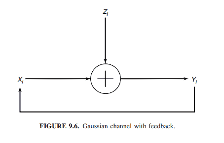
The Gaussian channel with feedback is illustrated in Figure 9.6. The output of the channel $Y_i$ is
$$
Y_i=X_i+Z_i, \quad Z_i \sim \mathcal{N}\left(0, K_Z^{(n)}\right) .
$$
The feedback allows the input of the channel to depend on the past values of the output.
A $\left(2^{n R}, n\right)$ code for the Gaussian channel with feedback consists of a sequence of mappings $x_i\left(W, Y^{i-1}\right)$, where $W \in\left{1,2, \ldots, 2^{n R}\right}$ is the input message and $Y^{i-1}$ is the sequence of past values of the output. Thus, $x(W, \cdot)$ is a code function rather than a codeword. In addition, we require that the code satisfy a power constraint,
$$
E\left[\frac{1}{n} \sum_{i=1}^n x_i^2\left(w, Y^{i-1}\right)\right] \leq P, \quad w \in\left{1,2, \ldots, 2^{n R}\right},
$$
where the expectation is over all possible noise sequences.
We characterize the capacity of the Gaussian channel is terms of the covariance matrices of the input $X$ and the noise $Z$. Because of the feedback, $X^n$ and $Z^n$ are not independent; $X_i$ depends causally on the past values of $Z$. In the next section we prove a converse for the Gaussian channel with feedback and show that we achieve capacity if we take $X$ to be Gaussian.
We now state an informal characterization of the capacity of the channel with and without feedback.
With feedback. The capacity $C_{n, \mathrm{FB}}$ in bits per transmission of the time-varying Gaussian channel with feedback is
$$
C_{n, \mathrm{FB}}=\max {\frac{1}{n} \operatorname{tr}\left(K_X^{(n)}\right) \leq P} \frac{1}{2 n} \log \frac{\left|K{X+Z}^{(n)}\right|}{\left|K_Z^{(n)}\right|}
$$
where the maximization is taken over all $X^n$ of the form
$$
X_i=\sum_{j=1}^{i-1} b_{i j} Z_j+V_i, \quad i=1,2, \ldots, n,
$$
and $V^n$ is independent of $Z^n$. To verify that the maximization over (9.101) involves no loss of generality, note that the distribution on $X^n+Z^n$ achieving the maximum entropy is Gaussian. Since $Z^n$ is also Gaussian, it can be verified that a jointly Gaussian distribution on $\left(X^n, Z^n, X^n+Z^n\right)$ achieves the maximization in (9.100). But since $Z^n=Y^n-X^n$, the most general jointly normal causal dependence of $X^n$ on $Y^n$ is of the form (9.101), where $V^n$ plays the role of the innovations process. Recasting (9.100) and (9.101) using $X=B Z+V$ and $Y=X+Z$, we can write
$$
C_{n, \mathrm{FB}}=\max \frac{1}{2 n} \log \frac{\left|(B+I) K_Z^{(n)}(B+I)^t+K_V\right|}{\left|K_Z^{(n)}\right|},
$$
where the maximum is taken over all nonnegative definite $K_V$ and strictly lower triangular $B$ such that
$$
\operatorname{tr}\left(B K_Z^{(n)} B^t+K_V\right) \leq n P .
$$
Note that $B$ is 0 if feedback is not allowed.
Without feedback. The capacity $C_n$ of the time-varying Gaussian channel without feedback is given by
$$
C_n=\max {\frac{1}{n} \operatorname{tr}\left(K_X^{(n)}\right) \leq P} \frac{1}{2 n} \log \frac{\left|K_X^{(n)}+K_Z^{(n)}\right|}{\left|K_Z^{(n)}\right|} . $$ This reduces to water-filling on the eigenvalues $\left{\lambda_i^{(n)}\right}$ of $K_Z^{(n)}$. Thus, $$ C_n=\frac{1}{2 n} \sum{i=1}^n \log \left(1+\frac{\left(\lambda-\lambda_i^{(n)}\right)^{+}}{\lambda_i^{(n)}}\right),
$$
where $(y)^{+}=\max {y, 0}$ and where $\lambda$ is chosen so that
$$
\sum_{i=1}^n\left(\lambda-\lambda_i^{(n)}\right)^{+}=n P
$$
We now prove an upper bound for the capacity of the Gaussian channel with feedback. This bound is actually achievable [136], and is therefore the capacity, but we do not prove this here.

信息论代写
数学代写|信息论代写information theory代考|CHANNELS WITH COLORED GAUSSIAN NOISE
在第9.4节中,我们考虑了一组平行独立高斯通道的情况,其中来自不同通道的噪声样本是独立的。现在我们将考虑噪声是相关的情况。这不仅代表了并行信道的情况,而且也代表了信道具有高斯噪声的情况。对于具有内存的信道,我们可以考虑将一个$n$连续使用的信道块视为$n$信道,并并行处理相关噪声。和第9.4节一样,我们将只计算这个通道的信息容量。
设$K_Z$为噪声的协方差矩阵,$K_X$为输入协方差矩阵。输入上的功率约束可以写成
$$
\frac{1}{n} \sum_i E X_i^2 \leq P,
$$
或者等价地,
$$
\frac{1}{n} \operatorname{tr}\left(K_X\right) \leq P .
$$
与第9.4节不同,这里的权力约束取决于$n$;必须为每个$n$计算容量。
就像在独立通道的情况下,我们可以写
$$
\begin{aligned}
I\left(X_1, X_2, \ldots, X_n ; Y_1, Y_2, \ldots, Y_n\right)= & h\left(Y_1, Y_2, \ldots, Y_n\right) \
& -h\left(Z_1, Z_2, \ldots, Z_n\right) .(9.81)
\end{aligned}
$$
这里$h\left(Z_1, Z_2, \ldots, Z_n\right)$仅由噪声的分布决定,而不依赖于输入分布的选择。所以求容量等于使$h\left(Y_1, Y_2, \ldots, Y_n\right)$最大化。输出的熵在$Y$正常时达到最大值,在输入正常时达到最大值。由于输入和噪声是独立的,输出的协方差$Y$为$K_Y=K_X+K_Z$,熵为
$$
h\left(Y_1, Y_2, \ldots, Y_n\right)=\frac{1}{2} \log \left((2 \pi e)^n\left|K_X+K_Z\right|\right)
$$
数学代写|信息论代写information theory代考|GAUSSIAN CHANNELS WITH FEEDBACK
然而,对于具有内存的信道,其中噪声从一个时刻到另一个时刻是相关的,反馈确实增加了容量。无反馈时的容量可以用充水法计算,但有反馈时的容量没有简单明确的表征。在本节中,我们用噪声的协方差矩阵$Z$描述容量的表达式。我们证明了这个容量表达式的一个逆表达式。然后,我们推导了由于反馈导致的容量增加的简单界。
带反馈的高斯信道如图9.6所示。通道$Y_i$的输出为
$$
Y_i=X_i+Z_i, \quad Z_i \sim \mathcal{N}\left(0, K_Z^{(n)}\right) .
$$
反馈允许通道的输入依赖于过去的输出值。
带有反馈的高斯信道的$\left(2^{n R}, n\right)$代码由映射序列$x_i\left(W, Y^{i-1}\right)$组成,其中$W \in\left{1,2, \ldots, 2^{n R}\right}$是输入消息,$Y^{i-1}$是过去输出值的序列。因此,$x(W, \cdot)$是一个代码函数,而不是一个码字。此外,我们要求代码满足功率约束,
$$
E\left[\frac{1}{n} \sum_{i=1}^n x_i^2\left(w, Y^{i-1}\right)\right] \leq P, \quad w \in\left{1,2, \ldots, 2^{n R}\right},
$$
期望大于所有可能的噪声序列。
我们用输入$X$和噪声$Z$的协方差矩阵来描述高斯信道的容量。因为反馈,$X^n$和$Z^n$不是独立的;$X_i$依赖于$Z$过去的值。在下一节中,我们将证明具有反馈的高斯信道的一个逆命题,并表明如果我们取$X$为高斯信道,我们将获得容量。
现在我们对有反馈和没有反馈的信道容量进行非正式表征。
有反馈。带反馈的时变高斯信道的传输容量$C_{n, \mathrm{FB}}$为
$$
C_{n, \mathrm{FB}}=\max {\frac{1}{n} \operatorname{tr}\left(K_X^{(n)}\right) \leq P} \frac{1}{2 n} \log \frac{\left|K{X+Z}^{(n)}\right|}{\left|K_Z^{(n)}\right|}
$$
在哪里最大化是采取了所有$X^n$的形式
$$
X_i=\sum_{j=1}^{i-1} b_{i j} Z_j+V_i, \quad i=1,2, \ldots, n,
$$
$V^n$独立于$Z^n$。为了验证(9.101)上的最大化不涉及一般性的损失,请注意$X^n+Z^n$上实现最大熵的分布是高斯分布。由于$Z^n$也是高斯分布,因此可以验证$\left(X^n, Z^n, X^n+Z^n\right)$上的联合高斯分布在(9.100)处达到最大值。但从$Z^n=Y^n-X^n$开始,$X^n$对$Y^n$最一般的联合正态因果关系是(9.101),其中$V^n$扮演创新过程的角色。使用$X=B Z+V$和$Y=X+Z$重铸(9.100)和(9.101),我们可以写
$$
C_{n, \mathrm{FB}}=\max \frac{1}{2 n} \log \frac{\left|(B+I) K_Z^{(n)}(B+I)^t+K_V\right|}{\left|K_Z^{(n)}\right|},
$$
这里的最大值是所有非负定的$K_V$和严格的下三角形$B$,这样
$$
\operatorname{tr}\left(B K_Z^{(n)} B^t+K_V\right) \leq n P .
$$
注意,如果不允许反馈,$B$为0。
没有反馈。无反馈时变高斯信道的容量$C_n$由式给出
$$
C_n=\max {\frac{1}{n} \operatorname{tr}\left(K_X^{(n)}\right) \leq P} \frac{1}{2 n} \log \frac{\left|K_X^{(n)}+K_Z^{(n)}\right|}{\left|K_Z^{(n)}\right|} . $$这简化为在$K_Z^{(n)}$的特征值$\left{\lambda_i^{(n)}\right}$上充水。因此,$$ C_n=\frac{1}{2 n} \sum{i=1}^n \log \left(1+\frac{\left(\lambda-\lambda_i^{(n)}\right)^{+}}{\lambda_i^{(n)}}\right),
$$
哪里是$(y)^{+}=\max {y, 0}$,哪里是$\lambda$
$$
\sum_{i=1}^n\left(\lambda-\lambda_i^{(n)}\right)^{+}=n P
$$
我们现在证明了带反馈的高斯信道容量的上界。这个界限实际上是可以达到的[136],因此是容量,但我们在这里不证明它。

统计代写请认准statistics-lab™. statistics-lab™为您的留学生涯保驾护航。
金融工程代写
金融工程是使用数学技术来解决金融问题。金融工程使用计算机科学、统计学、经济学和应用数学领域的工具和知识来解决当前的金融问题,以及设计新的和创新的金融产品。
非参数统计代写
非参数统计指的是一种统计方法,其中不假设数据来自于由少数参数决定的规定模型;这种模型的例子包括正态分布模型和线性回归模型。
广义线性模型代考
广义线性模型(GLM)归属统计学领域,是一种应用灵活的线性回归模型。该模型允许因变量的偏差分布有除了正态分布之外的其它分布。
术语 广义线性模型(GLM)通常是指给定连续和/或分类预测因素的连续响应变量的常规线性回归模型。它包括多元线性回归,以及方差分析和方差分析(仅含固定效应)。
有限元方法代写
有限元方法(FEM)是一种流行的方法,用于数值解决工程和数学建模中出现的微分方程。典型的问题领域包括结构分析、传热、流体流动、质量运输和电磁势等传统领域。
有限元是一种通用的数值方法,用于解决两个或三个空间变量的偏微分方程(即一些边界值问题)。为了解决一个问题,有限元将一个大系统细分为更小、更简单的部分,称为有限元。这是通过在空间维度上的特定空间离散化来实现的,它是通过构建对象的网格来实现的:用于求解的数值域,它有有限数量的点。边界值问题的有限元方法表述最终导致一个代数方程组。该方法在域上对未知函数进行逼近。[1] 然后将模拟这些有限元的简单方程组合成一个更大的方程系统,以模拟整个问题。然后,有限元通过变化微积分使相关的误差函数最小化来逼近一个解决方案。
tatistics-lab作为专业的留学生服务机构,多年来已为美国、英国、加拿大、澳洲等留学热门地的学生提供专业的学术服务,包括但不限于Essay代写,Assignment代写,Dissertation代写,Report代写,小组作业代写,Proposal代写,Paper代写,Presentation代写,计算机作业代写,论文修改和润色,网课代做,exam代考等等。写作范围涵盖高中,本科,研究生等海外留学全阶段,辐射金融,经济学,会计学,审计学,管理学等全球99%专业科目。写作团队既有专业英语母语作者,也有海外名校硕博留学生,每位写作老师都拥有过硬的语言能力,专业的学科背景和学术写作经验。我们承诺100%原创,100%专业,100%准时,100%满意。
随机分析代写
随机微积分是数学的一个分支,对随机过程进行操作。它允许为随机过程的积分定义一个关于随机过程的一致的积分理论。这个领域是由日本数学家伊藤清在第二次世界大战期间创建并开始的。
时间序列分析代写
随机过程,是依赖于参数的一组随机变量的全体,参数通常是时间。 随机变量是随机现象的数量表现,其时间序列是一组按照时间发生先后顺序进行排列的数据点序列。通常一组时间序列的时间间隔为一恒定值(如1秒,5分钟,12小时,7天,1年),因此时间序列可以作为离散时间数据进行分析处理。研究时间序列数据的意义在于现实中,往往需要研究某个事物其随时间发展变化的规律。这就需要通过研究该事物过去发展的历史记录,以得到其自身发展的规律。
回归分析代写
多元回归分析渐进(Multiple Regression Analysis Asymptotics)属于计量经济学领域,主要是一种数学上的统计分析方法,可以分析复杂情况下各影响因素的数学关系,在自然科学、社会和经济学等多个领域内应用广泛。
MATLAB代写
MATLAB 是一种用于技术计算的高性能语言。它将计算、可视化和编程集成在一个易于使用的环境中,其中问题和解决方案以熟悉的数学符号表示。典型用途包括:数学和计算算法开发建模、仿真和原型制作数据分析、探索和可视化科学和工程图形应用程序开发,包括图形用户界面构建MATLAB 是一个交互式系统,其基本数据元素是一个不需要维度的数组。这使您可以解决许多技术计算问题,尤其是那些具有矩阵和向量公式的问题,而只需用 C 或 Fortran 等标量非交互式语言编写程序所需的时间的一小部分。MATLAB 名称代表矩阵实验室。MATLAB 最初的编写目的是提供对由 LINPACK 和 EISPACK 项目开发的矩阵软件的轻松访问,这两个项目共同代表了矩阵计算软件的最新技术。MATLAB 经过多年的发展,得到了许多用户的投入。在大学环境中,它是数学、工程和科学入门和高级课程的标准教学工具。在工业领域,MATLAB 是高效研究、开发和分析的首选工具。MATLAB 具有一系列称为工具箱的特定于应用程序的解决方案。对于大多数 MATLAB 用户来说非常重要,工具箱允许您学习和应用专业技术。工具箱是 MATLAB 函数(M 文件)的综合集合,可扩展 MATLAB 环境以解决特定类别的问题。可用工具箱的领域包括信号处理、控制系统、神经网络、模糊逻辑、小波、仿真等。