标签: BSTA5014

统计代写|贝叶斯分析代写Bayesian Analysis代考|STAT4102

如果你也在 怎样代写贝叶斯分析Bayesian Analysis这个学科遇到相关的难题,请随时右上角联系我们的24/7代写客服。

贝叶斯分析,一种统计推断方法(以英国数学家托马斯-贝叶斯命名),允许人们将关于人口参数的先验信息与样本所含信息的证据相结合,以指导统计推断过程。

statistics-lab™ 为您的留学生涯保驾护航 在代写贝叶斯分析Bayesian Analysis方面已经树立了自己的口碑, 保证靠谱, 高质且原创的统计Statistics代写服务。我们的专家在代写贝叶斯分析Bayesian Analysis代写方面经验极为丰富,各种代写贝叶斯分析Bayesian Analysis相关的作业也就用不着说。

我们提供的贝叶斯分析Bayesian Analysis及其相关学科的代写,服务范围广, 其中包括但不限于:

  • Statistical Inference 统计推断
  • Statistical Computing 统计计算
  • Advanced Probability Theory 高等概率论
  • Advanced Mathematical Statistics 高等数理统计学
  • (Generalized) Linear Models 广义线性模型
  • Statistical Machine Learning 统计机器学习
  • Longitudinal Data Analysis 纵向数据分析
  • Foundations of Data Science 数据科学基础
统计代写|贝叶斯分析代写Bayesian Analysis代考|STAT4102

统计代写|贝叶斯分析代写Bayesian Analysis代考|Drug Testing

Here we dig deeper into the example (taken from Ziliak and McCloskey, 2008) first introduced in Chapter 2, Box 2.1. We are interested in comparing two weight-loss drugs to determine which should be sold. Experimental data on the drugs Oomph and Precision have shown that, over a one-month period for a number of test subjects:

  • Weight loss for Precision is approximately Normally distributed with mean 5 pounds and variance 1 . So we define the NPT for the node Precision as a Normal $(5,1)$ distribution.
  • Oomph showed a much higher average weight loss of 20 pounds but with much more variation and is estimated as a Normal $(20,100)$ distribution.
    We might be interested in two things here: one is predictability of the effect of a drug on weight loss and the other is the size or impact of the drug on weight loss. Let’s adopt a similar formulation to before:
    $$
    \begin{gathered}
    H_0: \text { Precision }>\text { Oomph } \
    H_1: \text { Oomph } \geq \text { Precision }
    \end{gathered}
    $$
    Figure 12.10 shows the AgenaRisk model used to test this hypothesis. Rather than create a node for the difference, Precision-Oomph, directly in AgenaRisk we have simply declared a single expression for the hypothesis node as
    if (Precision > Oomph, “Precision”, “Oomph”)
    rather than use two separate nodes as we did in the quality assurance example.

Notice that the hypothesis is approximately $93 \%$ in favor of Oomph over Precision, since only $7 \%$ of the time is Precision likely to result in more weight loss than Oomph. Interestingly we have included here two additional nodes to cover the risk that any of the drugs actually cause negative weight loss, that is, weight gain for the good reason that some may be fearful of putting on weight and might choose the drug that was less effective but also less risky. In this case someone might choose Precision since Oomph has a $2.28 \%$ chance of weight gain, where the chance of weight gain with Precision is negligible.
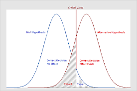
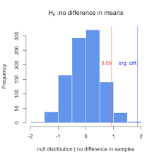
In the classical statistical approach to hypothesis testing in the drug testing example we would be interested in assessing the statistical significance of each drug with respect to its capability to reduce weight, that is, whether any weight reduction is likely to have occurred by chance. In doing this we compare the results for each drug against the null hypothesis: zero weight loss. So, for both Precision and Oomph we test the following hypotheses, where $\mu$ is the population mean weight loss in each case:
$$
\begin{aligned}
& H_0: \mu_0=0 \
& H_1: \mu_1>0
\end{aligned}
$$
Box 12.2 describes the classical statistical approach to testing this hypothesis in each case (i.e. the approach introduced in Section 12.2.1).

统计代写|贝叶斯分析代写Bayesian Analysis代考|Considering Difference between Distributions Rather Than Difference between Means

Consider the following problem scenario:
A new drug is trialled which is believed to increase survival time of patients with a particular disease. It is a comprehensive randomised control trial lasting 36 months in which 1000 patients with the disease take the drug and 1000 with the disease do not take the drug. The trial results show that the null hypothesis of “no increase in survival time” can be rejected with high confidence; specifically, there is greater than $99 \%$ chance that the mean survival time of people taking the drug is higher than those who do not. You are diagnosed with the disease. Should you take the drug and, if so, what are your chances of surviving longer if you do?
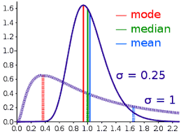
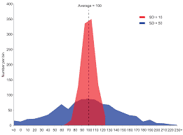
As in the previous problems we are comparing two attributes-the survival time with the drug and the survival time without the drug. Unfortunately, the $99 \%$ probability that the mean of the former is greater than the mean of the latter tells us nothing about the probability that any given person will survive longer if they take the drug. So, it does not help us to answer the question. The problem is that if we have reasonable size samples-as in this case-there will actually be very little uncertainty about the mean. All the “interesting” uncertainty is about the variance. As an extreme example suppose you could measure the height of every adult male in the United Kingdom. Then, despite wide variance in the results, the mean height will be an exact figure, say $176 \mathrm{~cm}$. Even if you were only able to take a sample of, say 100 , the mean of the sample would be a very accurate estimate of the true mean of 176 (i.e. with very little uncertainty). So, in the drug example, if the mean survival time of the 1000 patients taking the drug is 28.5 weeks, then this will be very close to the true, but unknown, survival time with little uncertainty. Yet the mean survival time will inevitably “hide” the fact that many of the patients survive the full 36 weeks while many die within the first 3 weeks.

Suppose that, based on the trial data, we get the following estimates for the mean and variance of the survival times:

Then we can construct the necessary $\mathrm{BN}$ model as shown in Figure 12.11.

The nodes with the estimated means and variances of the survival times are defined using the Normal distributions in the above table. Each of the “true” survival time nodes is defined simply as a Normal distribution with mean equal to the (parent) estimated mean and variance equal to the (parent) estimated variance. The Boolean node “Mean survival time no greater with drug” has its NPT defined as
if(mean_with > mean_without, ‘False’, ‘True’)
The Boolean node “survive no longer with drug” has its NPT defined as
if(with > without, ‘False’, ‘True’)
Note that the null hypothesis “Mean survival time no greater with drug” is easily rejected at the $1 \%$ level, and so the drug would certainly be accepted and recommended for patients with the disease. However, the situation for the null hypothesis “survive no longer with drug” is very different. There is actually a $47.45 \%$ chance that your survival time will be less if you take the drug than if you do not.

统计代写|贝叶斯分析代写Bayesian Analysis代考|STAT4102

贝叶斯分析代考

统计代写|贝叶斯分析代写Bayesian Analysis代考|Drug Testing

在这里,我们深入研究第 2 章专栏 2.1 中首次介绍的示例(取自 Ziliak 和 McCloskey,2008 年)。我 们有兴趣比较两种减肥药,以确定应该出售哪种。药物 Oomph 和 Precision 的实验数据表明,在一个 月的时间里,许多测试对象:

  • Precision 的体重减轻近似正态分布,均值为 5 磅,方差为 1 。所以我们将节点 Precision 的 NPT 定义为 $\operatorname{Normal}(5,1)$ 分配。
  • Oomph 表现出更高的平均体重减轻 20 磅,但变化更大,估计为正常 $(20,100)$ 分配。 我们可能对这里的两件事感兴趣:一是药物对减肥效果的可预测性,二是药物对减肥的大小或影 响。让我们采用与之前类似的公式:
    $$
    H_0: \text { Precision }>\text { Oomph } H_1: \text { Oomph } \geq \text { Precision }
    $$
    图 12.10 显示了用于检验该假设的 AgenaRisk 模型。我们没有直接在 AgenaRisk 中为差值 Precision-Oomph 创建一个节点,而是简单地为假设节点声明了一个表达式,就像 (Precision > Oomph, “Precision”, “Oomph”) 而不是像我们一样使用两个单独的节点在质量保证示例中做了。
    请注意,假设大约是 $93 \%$ 赞成 Oomph 而不是 Precision,因为只有 $7 \%$ 与 Oomph 相比,Precision 可 能会导致更多的体重减轻。有趣的是,我们在这里包括了两个额外的节点,以涵盖任何药物实际导致负 体重减轻的风险,即体重增加的充分理由是一些人可能害怕增加体重并可能选择效果较差的药物而且风 险也较小。在这种情况下,有人可能会选择 Precision,因为 Oomph 有 $2.28 \%$ 体重增加的机会,其中 Precision 增加体重的机会可以忽略不计。
    在药物测试示例中假设检验的经典统计方法中,我们有兴趣评估每种药物在其减肥能力方面的统计显着 性,即任何体重减轻是否可能是偶然发生的。在这样做时,我们将每种药物的结果与零假设进行比较: 体重减轻为零。因此,对于 Precision 和 Oomph,我们检验以下假设,其中 $\mu$ 是每种情况下的总体平均 体重减轻:
    $$
    H_0: \mu_0=0 \quad H_1: \mu_1>0
    $$
    专栏 12.2 描述了在每种情况下检验该假设的经典统计方法 (即第 12.2 .1 节中介绍的方法)。

统计代写|贝叶斯分析代写Bayesian Analysis代考|Considering Difference between Distributions Rather Than Difference between Means

考虑以下问题场景:
正在试用一种新药,据信它可以延长患有特定疾病的患者的生存时间。这是一项持续 36 个月的综合随机对照试验,其中 1000 名患有该疾病的患者服用该药物,1000 名患有该疾病的患者未服用该药物。试验结果表明,可以高置信度地拒绝“生存时间没有增加”的原假设;具体来说,有大于99%服用该药物的人的平均生存时间高于未服用药物的人的可能性。你被诊断出患有这种疾病。你应该服用这种药物吗?如果服用的话,你活得更久的机会有多大?
与前面的问题一样,我们正在比较两个属性——使用药物的生存时间和不使用药物的生存时间。不幸的是,99%前者的均值大于后者的均值的概率并没有告诉我们任何给定的人服用该药后活得更久的概率。所以,这并不能帮助我们回答这个问题。问题是,如果我们有合理大小的样本——就像在这种情况下——实际上平均值的不确定性很小。所有“有趣”的不确定性都与方差有关。举一个极端的例子,假设您可以测量英国每个成年男性的身高。然后,尽管结果差异很大,但平均身高将是一个精确的数字,比如176 C米. 即使您只能抽取 100 个样本,样本的均值也将是对 176 的真实均值的非常准确的估计(即不确定性很小)。因此,在药物示例中,如果服用该药物的 1000 名患者的平均生存时间为 28.5 周,那么这将非常接近真实但未知的生存时间,几乎没有不确定性。然而,平均生存时间将不可避免地“掩盖”一个事实,即许多患者存活了整整 36 周,而许多患者在前 3 周内死亡。

假设,根据试验数据,我们得到以下生存时间均值和方差的估计值:

然后我们可以构建必要的乙否模型如图 12.11 所示。

使用上表中的正态分布定义具有估计生存时间均值和方差的节点。每个“真实”生存时间节点都被简单地定义为均值等于(父)估计均值且方差等于(父)估计方差的正态分布。布尔节点“使用药物后平均生存时间不再延长”将其 NPT 定义为
if(mean_with > mean_without, ‘False’, ‘True’)
布尔节点“不再使用药物生存”将其 NPT 定义为
if(with > without, ‘False’, ‘True’)
请注意零假设“平均生存时间不超过药物”很容易被拒绝1%水平,因此该药物肯定会被接受并推荐给患有这种疾病的患者。然而,零假设“不再靠药物生存”的情况就大不相同了。实际上有一个47.45%如果您服药,您的生存时间可能会比您不服药时短。

统计代写|贝叶斯分析代写Bayesian Analysis代考 请认准statistics-lab™

统计代写请认准statistics-lab™. statistics-lab™为您的留学生涯保驾护航。

金融工程代写

金融工程是使用数学技术来解决金融问题。金融工程使用计算机科学、统计学、经济学和应用数学领域的工具和知识来解决当前的金融问题,以及设计新的和创新的金融产品。

非参数统计代写

非参数统计指的是一种统计方法,其中不假设数据来自于由少数参数决定的规定模型;这种模型的例子包括正态分布模型和线性回归模型。

广义线性模型代考

广义线性模型(GLM)归属统计学领域,是一种应用灵活的线性回归模型。该模型允许因变量的偏差分布有除了正态分布之外的其它分布。

术语 广义线性模型(GLM)通常是指给定连续和/或分类预测因素的连续响应变量的常规线性回归模型。它包括多元线性回归,以及方差分析和方差分析(仅含固定效应)。

有限元方法代写

有限元方法(FEM)是一种流行的方法,用于数值解决工程和数学建模中出现的微分方程。典型的问题领域包括结构分析、传热、流体流动、质量运输和电磁势等传统领域。

有限元是一种通用的数值方法,用于解决两个或三个空间变量的偏微分方程(即一些边界值问题)。为了解决一个问题,有限元将一个大系统细分为更小、更简单的部分,称为有限元。这是通过在空间维度上的特定空间离散化来实现的,它是通过构建对象的网格来实现的:用于求解的数值域,它有有限数量的点。边界值问题的有限元方法表述最终导致一个代数方程组。该方法在域上对未知函数进行逼近。[1] 然后将模拟这些有限元的简单方程组合成一个更大的方程系统,以模拟整个问题。然后,有限元通过变化微积分使相关的误差函数最小化来逼近一个解决方案。

tatistics-lab作为专业的留学生服务机构,多年来已为美国、英国、加拿大、澳洲等留学热门地的学生提供专业的学术服务,包括但不限于Essay代写,Assignment代写,Dissertation代写,Report代写,小组作业代写,Proposal代写,Paper代写,Presentation代写,计算机作业代写,论文修改和润色,网课代做,exam代考等等。写作范围涵盖高中,本科,研究生等海外留学全阶段,辐射金融,经济学,会计学,审计学,管理学等全球99%专业科目。写作团队既有专业英语母语作者,也有海外名校硕博留学生,每位写作老师都拥有过硬的语言能力,专业的学科背景和学术写作经验。我们承诺100%原创,100%专业,100%准时,100%满意。

随机分析代写


随机微积分是数学的一个分支,对随机过程进行操作。它允许为随机过程的积分定义一个关于随机过程的一致的积分理论。这个领域是由日本数学家伊藤清在第二次世界大战期间创建并开始的。

时间序列分析代写

随机过程,是依赖于参数的一组随机变量的全体,参数通常是时间。 随机变量是随机现象的数量表现,其时间序列是一组按照时间发生先后顺序进行排列的数据点序列。通常一组时间序列的时间间隔为一恒定值(如1秒,5分钟,12小时,7天,1年),因此时间序列可以作为离散时间数据进行分析处理。研究时间序列数据的意义在于现实中,往往需要研究某个事物其随时间发展变化的规律。这就需要通过研究该事物过去发展的历史记录,以得到其自身发展的规律。

回归分析代写

多元回归分析渐进(Multiple Regression Analysis Asymptotics)属于计量经济学领域,主要是一种数学上的统计分析方法,可以分析复杂情况下各影响因素的数学关系,在自然科学、社会和经济学等多个领域内应用广泛。

MATLAB代写

MATLAB 是一种用于技术计算的高性能语言。它将计算、可视化和编程集成在一个易于使用的环境中,其中问题和解决方案以熟悉的数学符号表示。典型用途包括:数学和计算算法开发建模、仿真和原型制作数据分析、探索和可视化科学和工程图形应用程序开发,包括图形用户界面构建MATLAB 是一个交互式系统,其基本数据元素是一个不需要维度的数组。这使您可以解决许多技术计算问题,尤其是那些具有矩阵和向量公式的问题,而只需用 C 或 Fortran 等标量非交互式语言编写程序所需的时间的一小部分。MATLAB 名称代表矩阵实验室。MATLAB 最初的编写目的是提供对由 LINPACK 和 EISPACK 项目开发的矩阵软件的轻松访问,这两个项目共同代表了矩阵计算软件的最新技术。MATLAB 经过多年的发展,得到了许多用户的投入。在大学环境中,它是数学、工程和科学入门和高级课程的标准教学工具。在工业领域,MATLAB 是高效研究、开发和分析的首选工具。MATLAB 具有一系列称为工具箱的特定于应用程序的解决方案。对于大多数 MATLAB 用户来说非常重要,工具箱允许您学习应用专业技术。工具箱是 MATLAB 函数(M 文件)的综合集合,可扩展 MATLAB 环境以解决特定类别的问题。可用工具箱的领域包括信号处理、控制系统、神经网络、模糊逻辑、小波、仿真等。

R语言代写问卷设计与分析代写
PYTHON代写回归分析与线性模型代写
MATLAB代写方差分析与试验设计代写
STATA代写机器学习/统计学习代写
SPSS代写计量经济学代写
EVIEWS代写时间序列分析代写
EXCEL代写深度学习代写
SQL代写各种数据建模与可视化代写

统计代写|贝叶斯分析代写Bayesian Analysis代考|MAST90125

如果你也在 怎样代写贝叶斯分析Bayesian Analysis这个学科遇到相关的难题,请随时右上角联系我们的24/7代写客服。

贝叶斯分析,一种统计推断方法(以英国数学家托马斯-贝叶斯命名),允许人们将关于人口参数的先验信息与样本所含信息的证据相结合,以指导统计推断过程。

statistics-lab™ 为您的留学生涯保驾护航 在代写贝叶斯分析Bayesian Analysis方面已经树立了自己的口碑, 保证靠谱, 高质且原创的统计Statistics代写服务。我们的专家在代写贝叶斯分析Bayesian Analysis代写方面经验极为丰富,各种代写贝叶斯分析Bayesian Analysis相关的作业也就用不着说。

我们提供的贝叶斯分析Bayesian Analysis及其相关学科的代写,服务范围广, 其中包括但不限于:

  • Statistical Inference 统计推断
  • Statistical Computing 统计计算
  • Advanced Probability Theory 高等概率论
  • Advanced Mathematical Statistics 高等数理统计学
  • (Generalized) Linear Models 广义线性模型
  • Statistical Machine Learning 统计机器学习
  • Longitudinal Data Analysis 纵向数据分析
  • Foundations of Data Science 数据科学基础
统计代写|贝叶斯分析代写Bayesian Analysis代考|MAST90125

统计代写|贝叶斯分析代写Bayesian Analysis代考|The Bayesian Approach Avoids p-Values Completely

What we really want to do is determine the probability that the null hypothesis is true given the data observed. This is precisely what the Bayesian approach provides. Moreover it enables us to:

  • Achieve a completely rational and unifying approach to hypothesis testing.
  • Avoid all ambiguity about the meaning of the null and alternative hypothesis, including what assumptions are being made about them.
  • Expose potential flaws in the classical approach.
  • Identify precisely what assumptions in the classical case are needed for it to “make sense.”
    The generic BN for the coin tossing hypothesis problem (which will enable us to capture every possible type of assumption and also extends to arbitrary number of coin tosses) is shown in Figure 12.3.

The Boolean nodes $H$ and ” $p H>0.5$ ?” – which would not normally be made explicit in a $\mathrm{BN}$ of this kind-are included since these are the nodes that clarify the assumptions being made in the different approaches. In a Bayesian approach we are allowed to condition the prior for the unknown $\mathrm{pH}$ on our background knowledge. Moreover, as we shall see, this is the (only) way of capturing exactly what we mean by a biased/non-biased coin. In the Bayesian approach we are also, of course, allowed to incorporate any prior knowledge about whether or not the coin is biased or not (although in most of what follows we will assume this is $50: 50$ ).

All of the key differences and assumptions are captured in the way we define the prior probability of node $\mathrm{pH}$ given the hypothesis. We consider some different possible assumptions in the following cases.

统计代写|贝叶斯分析代写Bayesian Analysis代考|Testing for Hypothetical Differences

The hypothesis concerns the probability of faultiness for each material, $p_A$ and $p_B$, respectively:
$$
\begin{aligned}
& H_0: p_A \geq p_B \
& H_1: p_A<p_B
\end{aligned}
$$
Let’s assume that the testing yielded 10 faults in 200 samples of material A and 15 faults in 200 samples of material B.

Before producing a solution here we first need to make an assumption about the prior probability of the materials being faulty. It seems reasonable to be indifferent here and select an ignorant prior where all probabilities of faultiness are equally likely. So we choose the Uniform $(0,1)$ distribution as the prior distribution for both $p_A$ and $p_B$. As we explained in Chapter 6 , the Binomial $(n, p)$ distribution (with $n$ equal to the number of samples and $p$ equal to the probability of faultiness) is a reasonable choice for modeling the likelihood of observing a number of faults in a sample of size $n$. We can use this for both material A and material B.
We can represent all of this information in a Bayesian network:

  • Clearly we need nodes $p_A$ and $p_B$ to represent the probability of faultiness for each of the materials (the node probability tables [NPTs] for these nodes will be the $\mathrm{U}(0,1)$ distribution).
  • We clearly also need nodes to represent the number of faults in the respective samples (the NPTs for these nodes will be the Binomial distributions).
    All that remains is to specify the nodes associated with our hypothesis. This is easily done by recasting the hypotheses as a difference, since $p_A \geq p_B$ is equivalent to $p_A-p_B \geq 0$ :
    $$
    \begin{aligned}
    & H_0: p_A-p_B \geq 0 \
    & H_1: p_A-p_B<0
    \end{aligned}
    $$
    We therefore need to add an additional node to represent the function $\left(p_A-p_B\right)$ with parent nodes $p_A$ and $p_B$, and a Boolean child node of $\left(p_A-p_B\right)$ to represent the hypothesis itself.

The resulting BN is shown in Figure 12.8 with the prior distribution for the hypothesis node displayed. As you can see the hypothesis is 50:50 for $H_0: H_1$.

We can now enter the testing data into the $\mathrm{BN}$ as evidence (shown in Figure 12.9) and can see that the distributions for $p_A, p_B$ and $\left(p_A-p_B\right)$ have all been updated and that the percentage probability that material $\mathrm{A}$ is better than material B is $84 \%$.

统计代写|贝叶斯分析代写Bayesian Analysis代考|MAST90125

贝叶斯分析代考

统计代写|贝叶斯分析代写Bayesian Analysis代考|The Bayesian Approach Avoids p-Values Completely

我们真正想做的是根据观察到的数据确定零假设为真的概率。这正是贝叶斯方法提供的。此外,它使我 们能够:

  • 实现一种完全理性和统一的假设检验方法。
  • 避免所有关于原假设和备择假设含义的歧义,包括对它们所做的假设。
  • 暴露经典方法中的潜在缺陷。
  • 准确确定经典案例中需要哪些假设才能使其“有意义”。
    图 12.3 显示了抛硬币假设问题的通用 BN (这将使我们能够捕获每一种可能的假设类型,并且还 可以扩展到任意数量的抛硬币)。
    布尔节点 $H$ 和” $p H>0.5$ ? – 通常不会在 $\mathrm{BN}$ 包括这种类型的节点,因为这些节点阐明了不同方法中所 做的假设。在贝叶斯方法中,我们可以为末知条件设定先验条件 $\mathrm{pH}$ 关于我们的背景知识。此外,正如我 们将看到的,这是 (唯一) 准确捕捉我们所说的有偏见/无偏见硬币的意思的方法。当然,在贝叶斯方法 中,我们也可以结合任何关于硬币是否有偏差的先验知识(尽管在接下来的大部分内容中我们会假设这 是 $50: 50)$.
    我们定义节点先验概率的方式捕获了所有关键差异和假设 $\mathrm{pH}$ 给定假设。我们在以下情况下考虑一些不同 的可能假设。

统计代写|贝叶斯分析代写Bayesian Analysis代考|Testing for Hypothetical Differences

该假设涉及每种材料的缺陷概率, $p_A$ 和 $p_B$ ,分别:
$$
H_0: p_A \geq p_B \quad H_1: p_A<p_B
$$
假设测试在 200 个材料 $\mathrm{A}$ 样本中产生 10 个故障,在 200 个材料 $\mathrm{B}$ 样本中产生 15 个故障。
在此处生成解决方案之前,我们首先需要假设材料有缺陷的先验概率。在这里漠不关心并选择一个无知 的先验似乎是合理的,在这个先验中所有的错误概率都是同样可能的。所以我们选择Uniform $(0,1)$ 分布 作为两者的先验分布 $p_A$ 和 $p_B$. 正如我们在第 6 章中解释的那样,二项式 $(n, p)$ 分布(与 $n$ 等于样本数和 $p$ 等于故障概率)是一个合理的选择,用于模拟在一个大小的样本中观察到多个故障的可能性 $n$. 我们可 以将其用于材料 $A$ 和材料 $B$ 。
我们可以在贝叶斯网络中表示所有这些信息:

  • 显然我们需要节点 $p_A$ 和 $p_B$ 表示每种材料的故障概率(这些节点的节点概率表 [NPTs] 将是U $\mathrm{U}(0,1)$ 分配)。
  • 我们显然还需要节点来表示各个样本中的故障数量(这些节点的 NPT 将是二项分布)。 剩下的就是指定与我们的假设相关的节点。这很容易通过将假设重铸为差异来完成,因为 $p_A \geq p_B$ 相当于 $p_A-p_B \geq 0$ :
    $$
    H_0: p_A-p_B \geq 0 \quad H_1: p_A-p_B<0
    $$
    因此,我们需要添加一个额外的节点来表示函数 $\left(p_A-p_B\right)$ 与父节点 $p_A$ 和 $p_B$ ,和一个布尔子节点 $\left(p_A-p_B\right)$ 代表假设本身。
    生成的 BN 如图 12.8 所示,其中显示了假设节点的先验分布。如您所见,假设是 50:50 $H_0: H_1$.
    我们现在可以将测试数据输入到 $\mathrm{BN}$ 作为证据(如图 12.9 所示),可以看出 $p_A, p_B$ 和 $\left(p_A-p_B\right)$ 已经 全部更新,并且该材料的百分比概率 $\mathrm{A}$ 比材料 $\mathrm{B}$ 好 $84 \%$.
统计代写|贝叶斯分析代写Bayesian Analysis代考 请认准statistics-lab™

统计代写请认准statistics-lab™. statistics-lab™为您的留学生涯保驾护航。

金融工程代写

金融工程是使用数学技术来解决金融问题。金融工程使用计算机科学、统计学、经济学和应用数学领域的工具和知识来解决当前的金融问题,以及设计新的和创新的金融产品。

非参数统计代写

非参数统计指的是一种统计方法,其中不假设数据来自于由少数参数决定的规定模型;这种模型的例子包括正态分布模型和线性回归模型。

广义线性模型代考

广义线性模型(GLM)归属统计学领域,是一种应用灵活的线性回归模型。该模型允许因变量的偏差分布有除了正态分布之外的其它分布。

术语 广义线性模型(GLM)通常是指给定连续和/或分类预测因素的连续响应变量的常规线性回归模型。它包括多元线性回归,以及方差分析和方差分析(仅含固定效应)。

有限元方法代写

有限元方法(FEM)是一种流行的方法,用于数值解决工程和数学建模中出现的微分方程。典型的问题领域包括结构分析、传热、流体流动、质量运输和电磁势等传统领域。

有限元是一种通用的数值方法,用于解决两个或三个空间变量的偏微分方程(即一些边界值问题)。为了解决一个问题,有限元将一个大系统细分为更小、更简单的部分,称为有限元。这是通过在空间维度上的特定空间离散化来实现的,它是通过构建对象的网格来实现的:用于求解的数值域,它有有限数量的点。边界值问题的有限元方法表述最终导致一个代数方程组。该方法在域上对未知函数进行逼近。[1] 然后将模拟这些有限元的简单方程组合成一个更大的方程系统,以模拟整个问题。然后,有限元通过变化微积分使相关的误差函数最小化来逼近一个解决方案。

tatistics-lab作为专业的留学生服务机构,多年来已为美国、英国、加拿大、澳洲等留学热门地的学生提供专业的学术服务,包括但不限于Essay代写,Assignment代写,Dissertation代写,Report代写,小组作业代写,Proposal代写,Paper代写,Presentation代写,计算机作业代写,论文修改和润色,网课代做,exam代考等等。写作范围涵盖高中,本科,研究生等海外留学全阶段,辐射金融,经济学,会计学,审计学,管理学等全球99%专业科目。写作团队既有专业英语母语作者,也有海外名校硕博留学生,每位写作老师都拥有过硬的语言能力,专业的学科背景和学术写作经验。我们承诺100%原创,100%专业,100%准时,100%满意。

随机分析代写


随机微积分是数学的一个分支,对随机过程进行操作。它允许为随机过程的积分定义一个关于随机过程的一致的积分理论。这个领域是由日本数学家伊藤清在第二次世界大战期间创建并开始的。

时间序列分析代写

随机过程,是依赖于参数的一组随机变量的全体,参数通常是时间。 随机变量是随机现象的数量表现,其时间序列是一组按照时间发生先后顺序进行排列的数据点序列。通常一组时间序列的时间间隔为一恒定值(如1秒,5分钟,12小时,7天,1年),因此时间序列可以作为离散时间数据进行分析处理。研究时间序列数据的意义在于现实中,往往需要研究某个事物其随时间发展变化的规律。这就需要通过研究该事物过去发展的历史记录,以得到其自身发展的规律。

回归分析代写

多元回归分析渐进(Multiple Regression Analysis Asymptotics)属于计量经济学领域,主要是一种数学上的统计分析方法,可以分析复杂情况下各影响因素的数学关系,在自然科学、社会和经济学等多个领域内应用广泛。

MATLAB代写

MATLAB 是一种用于技术计算的高性能语言。它将计算、可视化和编程集成在一个易于使用的环境中,其中问题和解决方案以熟悉的数学符号表示。典型用途包括:数学和计算算法开发建模、仿真和原型制作数据分析、探索和可视化科学和工程图形应用程序开发,包括图形用户界面构建MATLAB 是一个交互式系统,其基本数据元素是一个不需要维度的数组。这使您可以解决许多技术计算问题,尤其是那些具有矩阵和向量公式的问题,而只需用 C 或 Fortran 等标量非交互式语言编写程序所需的时间的一小部分。MATLAB 名称代表矩阵实验室。MATLAB 最初的编写目的是提供对由 LINPACK 和 EISPACK 项目开发的矩阵软件的轻松访问,这两个项目共同代表了矩阵计算软件的最新技术。MATLAB 经过多年的发展,得到了许多用户的投入。在大学环境中,它是数学、工程和科学入门和高级课程的标准教学工具。在工业领域,MATLAB 是高效研究、开发和分析的首选工具。MATLAB 具有一系列称为工具箱的特定于应用程序的解决方案。对于大多数 MATLAB 用户来说非常重要,工具箱允许您学习应用专业技术。工具箱是 MATLAB 函数(M 文件)的综合集合,可扩展 MATLAB 环境以解决特定类别的问题。可用工具箱的领域包括信号处理、控制系统、神经网络、模糊逻辑、小波、仿真等。

R语言代写问卷设计与分析代写
PYTHON代写回归分析与线性模型代写
MATLAB代写方差分析与试验设计代写
STATA代写机器学习/统计学习代写
SPSS代写计量经济学代写
EVIEWS代写时间序列分析代写
EXCEL代写深度学习代写
SQL代写各种数据建模与可视化代写

统计代写|贝叶斯分析代写Bayesian Analysis代考|MAST90125

如果你也在 怎样代写贝叶斯分析Bayesian Analysis这个学科遇到相关的难题,请随时右上角联系我们的24/7代写客服。

贝叶斯分析,一种统计推断方法(以英国数学家托马斯-贝叶斯命名),允许人们将关于人口参数的先验信息与样本所含信息的证据相结合,以指导统计推断过程。

statistics-lab™ 为您的留学生涯保驾护航 在代写贝叶斯分析Bayesian Analysis方面已经树立了自己的口碑, 保证靠谱, 高质且原创的统计Statistics代写服务。我们的专家在代写贝叶斯分析Bayesian Analysis代写方面经验极为丰富,各种代写贝叶斯分析Bayesian Analysis相关的作业也就用不着说。

我们提供的贝叶斯分析Bayesian Analysis及其相关学科的代写,服务范围广, 其中包括但不限于:

  • Statistical Inference 统计推断
  • Statistical Computing 统计计算
  • Advanced Probability Theory 高等概率论
  • Advanced Mathematical Statistics 高等数理统计学
  • (Generalized) Linear Models 广义线性模型
  • Statistical Machine Learning 统计机器学习
  • Longitudinal Data Analysis 纵向数据分析
  • Foundations of Data Science 数据科学基础
统计代写|贝叶斯分析代写Bayesian Analysis代考|MAST90125

统计代写|贝叶斯分析代写Bayesian Analysis代考|The Danger of Averages

Fred and Jane study on the same course spread over two years. To complete the course they have to complete 10 modules. At the end, their average annual results are as shown in Table 2.7. Jane’s scores are worse than Fred’s every year. So how is it possible that Jane got the prize for the student with the best grade? It is because the overall average figure is an average of the year averages rather than an average over all 10 modules. We cannot work out the average for the 10 modules unless we know how many modules each student takes in each year.
In fact:

  • Fred took 7 modules in Year 1 and 3 modules in Year 2
  • Jane took 2 modules in Year 1 and 8 modules in Year 2.
    Assuming each module is marked out of 100 , we can use this information to compute the total scores as shown in Table 2.8. So clearly Jane did better overall than Fred.

This is an example of Simpson’s paradox. It seems like a paradoxFred’s average marks are consistently higher than Jane’s average marks but Jane’s overall average is higher. But it is not really a paradox. It is simply a mistake to assume that you can take an average of averages without (in this case) taking account of the number of modules that make up each average.

Look at it the following way and it all becomes clear: In the year when Fred did the bulk of his modules he averaged 50; in the year when Jane did the bulk of her modules she averaged 62 . When you look at it that way it is not such a surprise that Jane did better overall.

This type of instance of Simpson’s paradox is particularly common in medical studies. Consider the example shown in Tables 2.9-2.11 (based on a simplified version of a study described in Bishop et al., 1975) in which the indications from the overall aggregated data from a number of clinics (Table 2.9) suggest a positive association between pre-natal care and infant survival rate. However, when the data are analysed for each individual clinic (Tables 2.10-2.11) the survival rate is actually lower when pre-natal care is provided in each case. Bishop et al. concluded:
“If we were to look at this [combined] table we would erroneously conclude that survival was related to the amount of care received.”

统计代写|贝叶斯分析代写Bayesian Analysis代考|What Type of Average?

When we used the average for the exam marks data above we were actually using one particular (most commonly used) measure of average: the mean. This is defined as the sum of all the data point values divided by the number of data points.

But it is not the only measure of average. Another important measure of average is the median. If you put all the data point values in order from lowest to highest then the median is the value directly in the middle, that is, it is the value for which half the data points lie below and half lie above.
Since critical decisions are often made based on knowledge only of the average of some key value, it is important to understand the extent to which the mean and median can differ for the same data. Take a look at Figure 2.21. This shows the percentage distribution of salaries (in \$) for workers in one city.

Note that the vast majority of the population (83\%) have salaries within a fairly narrow range $(\$ 10,000-\$ 50,000)$. But $2 \%$ have salaries in excess of $\$ 1$ million. The effect of this asymmetry in the distribution is that the median salary is $\$ 23,000$, whereas the mean is $\$ 137,000$. By definition half of the population earn at least the median salary; but just $5 \%$ of the population earn at least the mean salary.

Of course, the explanation for this massive difference is the “long tail” of the distribution. A small number of very high earners massively skew the mean figure. Nevertheless, for readers brought up on the notion that most data is inherently bell-shaped (i.e. a Normal distribution in the sense explained in Section 2.1) this difference between the mean and median will come as a surprise. In Normal distributions the mean and median are always equal, and in those cases you do not therefore need to worry about how you measure average.

The ramifications in decision making of failing to understand the difference between different measures of average can be devastating.

统计代写|贝叶斯分析代写Bayesian Analysis代考|MAST90125

贝叶斯分析代考

统计代写|贝叶斯分析代写Bayesian Analysis代考|The Danger of Averages

弗雷德和简在两年时间里学习了同一门课程。要完成课程,他们必须完成 10 个模块。最后,他们的年均结果如表2.7所示。简的成绩每年都比弗雷德差。那么,简怎么可能获得成绩最好的学生的奖品呢?这是因为总体平均数是年度平均数的平均数,而不是所有 10 个模块的平均数。除非我们知道每个学生每年学习多少个模块,否则我们无法计算出这 10 个模块的平均值。
实际上:

  • Fred 在第 1 年学习了 7 个模块,在第 2 年学习了 3 个模块
  • Jane 在第 1 年选修了 2 个模块,在第 2 年选修了 8 个模块。
    假设每个模块都被标记为满分 100,我们可以使用此信息来计算总分,如表 2.8 所示。很明显,简总体上比弗雷德做得更好。

这是辛普森悖论的一个例子。这似乎是一个悖论 Fred 的平均分一直高于 Jane 的平均分,但 Jane 的总体平均分更高。但这并不是真正的悖论。假设您可以在不考虑(在这种情况下)构成每个平均值的模块数量的情况下取平均数,这是完全错误的。

从下面的角度来看,一切都会变得清晰起来:在 Fred 完成大部分模块的那一年,他的平均得分为 50;在简完成大部分模块的那一年,她的平均成绩为 62 分。当你以这种方式看待它时,简的整体表现更好就不足为奇了。

这种辛普森悖论的例子在医学研究中尤为常见。考虑表 2.9-2.11 中显示的示例(基于 Bishop 等人,1975 年描述的一项研究的简化版本),其中来自许多诊所的总体汇总数据(表 2.9)的指示表明两者之间存在正相关产前护理和婴儿存活率。然而,当对每个诊所的数据进行分析时(表 2.10-2.11),在每个案例中提供产前护理时,存活率实际上较低。主教等。总结道:
“如果我们查看这张 [组合] 表,我们会错误地得出结论,认为生存与接受的护理量有关。”

统计代写|贝叶斯分析代写Bayesian Analysis代考|What Type of Average?

当我们对上面的考试分数数据使用平均值时,我们实际上使用了一种特定的(最常用的)平均值度量:平均值。这被定义为所有数据点值的总和除以数据点的数量。

但这并不是平均水平的唯一衡量标准。平均数的另一个重要衡量标准是中位数。如果将所有数据点值按从低到高的顺序排列,则中位数就是正中间的值,也就是说,它是一半数据点在下方,一半在上方的值。
由于关键决策通常仅基于对某些关键值的平均值的了解,因此了解相同数据的均值和中值的差异程度非常重要。看一下图 2.21。这显示了一个城市中工人的工资(以$ 为单位)的百分比分布。

请注意,绝大多数人 (83\%) 的薪水都在相当狭窄的范围内($10,000−$50,000). 但2%工资超过$1百万。这种分布不对称的影响是工资中位数是$23,000, 而平均值是$137,000. 根据定义,一半的人口至少赚取中位数工资;只是5%的人口至少赚取平均工资。

当然,造成这种巨大差异的原因是分布的“长尾”。少数非常高的收入者极大地扭曲了平均数字。然而,对于提出大多数数据本质上是钟形(即第 2.1 节中解释的正态分布)这一概念的读者来说,均值和中位数之间的这种差异会令人惊讶。在正态分布中,均值和中位数总是相等的,因此在这种情况下,您无需担心如何衡量平均值。

未能理解不同平均值测量之间的差异在决策过程中的后果可能是毁灭性的。

统计代写|贝叶斯分析代写Bayesian Analysis代考 请认准statistics-lab™

统计代写请认准statistics-lab™. statistics-lab™为您的留学生涯保驾护航。

金融工程代写

金融工程是使用数学技术来解决金融问题。金融工程使用计算机科学、统计学、经济学和应用数学领域的工具和知识来解决当前的金融问题,以及设计新的和创新的金融产品。

非参数统计代写

非参数统计指的是一种统计方法,其中不假设数据来自于由少数参数决定的规定模型;这种模型的例子包括正态分布模型和线性回归模型。

广义线性模型代考

广义线性模型(GLM)归属统计学领域,是一种应用灵活的线性回归模型。该模型允许因变量的偏差分布有除了正态分布之外的其它分布。

术语 广义线性模型(GLM)通常是指给定连续和/或分类预测因素的连续响应变量的常规线性回归模型。它包括多元线性回归,以及方差分析和方差分析(仅含固定效应)。

有限元方法代写

有限元方法(FEM)是一种流行的方法,用于数值解决工程和数学建模中出现的微分方程。典型的问题领域包括结构分析、传热、流体流动、质量运输和电磁势等传统领域。

有限元是一种通用的数值方法,用于解决两个或三个空间变量的偏微分方程(即一些边界值问题)。为了解决一个问题,有限元将一个大系统细分为更小、更简单的部分,称为有限元。这是通过在空间维度上的特定空间离散化来实现的,它是通过构建对象的网格来实现的:用于求解的数值域,它有有限数量的点。边界值问题的有限元方法表述最终导致一个代数方程组。该方法在域上对未知函数进行逼近。[1] 然后将模拟这些有限元的简单方程组合成一个更大的方程系统,以模拟整个问题。然后,有限元通过变化微积分使相关的误差函数最小化来逼近一个解决方案。

tatistics-lab作为专业的留学生服务机构,多年来已为美国、英国、加拿大、澳洲等留学热门地的学生提供专业的学术服务,包括但不限于Essay代写,Assignment代写,Dissertation代写,Report代写,小组作业代写,Proposal代写,Paper代写,Presentation代写,计算机作业代写,论文修改和润色,网课代做,exam代考等等。写作范围涵盖高中,本科,研究生等海外留学全阶段,辐射金融,经济学,会计学,审计学,管理学等全球99%专业科目。写作团队既有专业英语母语作者,也有海外名校硕博留学生,每位写作老师都拥有过硬的语言能力,专业的学科背景和学术写作经验。我们承诺100%原创,100%专业,100%准时,100%满意。

随机分析代写


随机微积分是数学的一个分支,对随机过程进行操作。它允许为随机过程的积分定义一个关于随机过程的一致的积分理论。这个领域是由日本数学家伊藤清在第二次世界大战期间创建并开始的。

时间序列分析代写

随机过程,是依赖于参数的一组随机变量的全体,参数通常是时间。 随机变量是随机现象的数量表现,其时间序列是一组按照时间发生先后顺序进行排列的数据点序列。通常一组时间序列的时间间隔为一恒定值(如1秒,5分钟,12小时,7天,1年),因此时间序列可以作为离散时间数据进行分析处理。研究时间序列数据的意义在于现实中,往往需要研究某个事物其随时间发展变化的规律。这就需要通过研究该事物过去发展的历史记录,以得到其自身发展的规律。

回归分析代写

多元回归分析渐进(Multiple Regression Analysis Asymptotics)属于计量经济学领域,主要是一种数学上的统计分析方法,可以分析复杂情况下各影响因素的数学关系,在自然科学、社会和经济学等多个领域内应用广泛。

MATLAB代写

MATLAB 是一种用于技术计算的高性能语言。它将计算、可视化和编程集成在一个易于使用的环境中,其中问题和解决方案以熟悉的数学符号表示。典型用途包括:数学和计算算法开发建模、仿真和原型制作数据分析、探索和可视化科学和工程图形应用程序开发,包括图形用户界面构建MATLAB 是一个交互式系统,其基本数据元素是一个不需要维度的数组。这使您可以解决许多技术计算问题,尤其是那些具有矩阵和向量公式的问题,而只需用 C 或 Fortran 等标量非交互式语言编写程序所需的时间的一小部分。MATLAB 名称代表矩阵实验室。MATLAB 最初的编写目的是提供对由 LINPACK 和 EISPACK 项目开发的矩阵软件的轻松访问,这两个项目共同代表了矩阵计算软件的最新技术。MATLAB 经过多年的发展,得到了许多用户的投入。在大学环境中,它是数学、工程和科学入门和高级课程的标准教学工具。在工业领域,MATLAB 是高效研究、开发和分析的首选工具。MATLAB 具有一系列称为工具箱的特定于应用程序的解决方案。对于大多数 MATLAB 用户来说非常重要,工具箱允许您学习应用专业技术。工具箱是 MATLAB 函数(M 文件)的综合集合,可扩展 MATLAB 环境以解决特定类别的问题。可用工具箱的领域包括信号处理、控制系统、神经网络、模糊逻辑、小波、仿真等。

R语言代写问卷设计与分析代写
PYTHON代写回归分析与线性模型代写
MATLAB代写方差分析与试验设计代写
STATA代写机器学习/统计学习代写
SPSS代写计量经济学代写
EVIEWS代写时间序列分析代写
EXCEL代写深度学习代写
SQL代写各种数据建模与可视化代写

统计代写|贝叶斯分析代写Bayesian Analysis代考|STAT4102

如果你也在 怎样代写贝叶斯分析Bayesian Analysis这个学科遇到相关的难题,请随时右上角联系我们的24/7代写客服。

贝叶斯分析,一种统计推断方法(以英国数学家托马斯-贝叶斯命名),允许人们将关于人口参数的先验信息与样本所含信息的证据相结合,以指导统计推断过程。

statistics-lab™ 为您的留学生涯保驾护航 在代写贝叶斯分析Bayesian Analysis方面已经树立了自己的口碑, 保证靠谱, 高质且原创的统计Statistics代写服务。我们的专家在代写贝叶斯分析Bayesian Analysis代写方面经验极为丰富,各种代写贝叶斯分析Bayesian Analysis相关的作业也就用不着说。

我们提供的贝叶斯分析Bayesian Analysis及其相关学科的代写,服务范围广, 其中包括但不限于:

  • Statistical Inference 统计推断
  • Statistical Computing 统计计算
  • Advanced Probability Theory 高等概率论
  • Advanced Mathematical Statistics 高等数理统计学
  • (Generalized) Linear Models 广义线性模型
  • Statistical Machine Learning 统计机器学习
  • Longitudinal Data Analysis 纵向数据分析
  • Foundations of Data Science 数据科学基础
统计代写|贝叶斯分析代写Bayesian Analysis代考|STAT4102

统计代写|贝叶斯分析代写Bayesian Analysis代考|The Shotgun Fallacy

Let us suppose that we are interested in possible “causes” of student exam success. To make our example as simple as possible let us assume that exam scores are measured on a scale of 1 (worst) to 10 (best).

Now let us think of a number of possible “causes” of exam success. These could include plausible factors like coursework score and class attendance. But we could also throw in some implausible factors like the number of sexual partners, number of football matches attended, or number of potatoes eaten on 12 January. In fact, to effectively demonstrate the point let us only consider a set of totally implausible factors. For simplicity we will assume that, like the exam score, they can all be measured on a scale of 1 to 10 .

Now although these factors-suppose we think of 18-are completely silly, let’s actually remove any possibility that they are in any way valid factors by generating the results for them purely randomly. You can do this yourself. Create an Excel spreadsheet and type the entry =RANDBETWEEN $(1,10)$ into cell A1. This will generate a random number between 1 and 10. By copying and pasting this entry create a set of random numbers like the set shown in Figure 2.16. There are 18 columns (A through to R) that we can think of as being the 18 silly factors associated with the students. We have also added column $\mathrm{S}$, which represents the student exam score, again generated randomly in the same way.
Now, using Excel’s built-in data analysis package, run a correlation analysis for each column (A through R) against the exam score (column S). If the correlation coefficient is higher than $0.561$ then the correlation is considered to be highly significant (the $p$-value is $0.01$ ).
In fact, because of the number of factors we are trying here it is very likely that you will find at least one column for which there is a significant correlation with $S$. In Figure $2.16$ the correlation coefficient of $\mathrm{H}$ and $\mathrm{S}$ is $0.59$. Since column $\mathrm{H}$ is just as likely to represent number of potatoes eaten on 12 January as any other factor, would we be correct in concluding that eating potatoes on 12 January is the key to exam success?

In fact, because of the number of factors, it is also almost certain that among the 18 factors themselves you will also find at least two pairs that have a significant correlation. For example, in this case columns $B$ and $Q$ have a correlation coefficient of $0.62$, which apparently might lead us to conclude that you can increase the number of football matches you attend by taking on more sexual partners.

统计代写|贝叶斯分析代写Bayesian Analysis代考|The Danger of Regression

Suppose that you are blowing up a large balloon. After each puff you measure the surface area and record it as shown in Figure 2.17. So, after the 23 rd puff the surface is $181 \mathrm{sq} \mathrm{cm}$. What will the surface area be on the 24th puff? On the 50th puff?

As opposed to the data on growth rates in Section 2.1, there is no doubt that the data here exhibits a clear trend. When presented with this kind of problem professionals often try to find lines that best fit the historical trend. As we saw in Section $2.3$ this is an example of regression analysis. As in the road fatalities example there, the simplest (and most common) approach is to assume a simple straight line fit (called linear regression), producing a line such as line A shown in Figure 2.18. Alternatively, we might decide that the relative slow down of increase toward the end of the data is indicative of a curve such as line B (this is an example of nonlinear regression). The lines provide us with a method of predicting future values. The line A fit results in a prediction of 186 for the 24th puff, whereas the line B fit results in a prediction of 183.

It is also common for analysts to apply what are called time-series adjustments into their prediction to take account of the fact that there are local sequential differences; in this case the even-numbered puffs tend to result in lower increases than the odd-numbered puffs (for the simple reason that we blow harder on alternative puffs). Factoring in the time-series analysis results in an adjusted prediction of 184 for puff 24 in the linear regression and 182 in the quadratic regression. Predictions further ahead, such as at puff 30 , are farther apart ( 235 for line A and 185 for line B).

As we saw in Section $2.1$ it was for reasons quite similar to this that the traditional statistical models were unable to predict the collapse of the banking sector in 2008 that ushered in a major worldwide recession. Although the models can incorporate millions of historical data to produce highly complex-and accurate-predictions over the short term during periods of growth, they were predicated on a set of barely articulated overoptimistic assumptions. The most basic knowledge about balloons would have indicated that a complete burst was inevitable, but traditional statistical models cannot incorporate this knowledge. Failure to do so is an example of what is commonly called the fallacy of induction. A similar example is highlighted in the Sidebar $2.4$.

统计代写|贝叶斯分析代写Bayesian Analysis代考|STAT4102

贝叶斯分析代考

统计代写|贝叶斯分析代写Bayesian Analysis代考|The Shotgun Fallacy

假设我们对学生考试成功的可能“原因”感兴趣。为了让我们的例子尽可能简单,让我们假设考试成绩是按照 1(最差)到 10(最好)的等级来衡量的。

现在让我们想一想考试成功的一些可能“原因”。这些可能包括合理的因素,如课程作业分数和课堂出勤率。但我们也可以加入一些难以置信的因素,例如性伴侣的数量、参加的足球比赛的数量或 1 月 12 日吃的土豆数量。事实上,为了有效地证明这一点,让我们只考虑一组完全难以置信的因素。为简单起见,我们假设它们与考试成绩一样,都可以用 1 到 10 的等级来衡量。

现在,尽管这些因素(假设我们认为是 18 个)完全是愚蠢的,但实际上让我们通过纯随机生成结果来消除它们在任何方面都是有效因素的任何可能性。你可以自己做。创建 Excel 电子表格并键入条目 =RANDBETWEEN(1,10)进入单元格A1。这将生成一个介于 1 和 10 之间的随机数。通过复制和粘贴此条目创建一组随机数,如图 2.16 所示。我们可以将 18 列(A 到 R)视为与学生相关的 18 个愚蠢因素。我们还添加了专栏小号,代表学生的考试成绩,同样以同样的方式随机生成。
现在,使用 Excel 的内置数据分析包,对每一列(A 到 R)与考试分数(S 列)进行相关性分析。如果相关系数高于0.561那么相关性被认为是非常显着的(p-价值是0.01).
事实上,由于我们在这里尝试的因素数量众多,您很可能会发现至少一列与小号. 在图中2.16的相关系数H和小号是0.59. 自列H与任何其他因素一样可能代表 1 月 12 日吃的土豆数量,我们得出 1 月 12 日吃土豆是考试成功的关键的结论是否正确?

事实上,由于因素的数量,几乎可以肯定的是,在 18 个因素本身中,你还会发现至少两个具有显着相关性的因素。例如,在这种情况下列乙和问具有相关系数0.62,这显然可能会让我们得出结论,你可以通过接受更多的性伴侣来增加你参加的足球比赛的数量。

统计代写|贝叶斯分析代写Bayesian Analysis代考|The Danger of Regression

假设你正在吹一个大气球。每次抽吸后,您测量表面积并记录下来,如图 2.17 所示。所以,在第 23 次抽吸之后,表面是181秒qC米. 第 24 次抽吸的表面积是多少?第 50 口?

相对于2.1节的增长率数据,毫无疑问,这里的数据呈现出明显的趋势。当遇到此类问题时,专业人士通常会尝试找到最符合历史趋势的路线。正如我们在部分中看到的2.3这是回归分析的一个例子。就像那里的道路死亡案例一样,最简单(也是最常见)的方法是假设一个简单的直线拟合(称为线性回归),生成一条线,如图 2.18 中所示的线 A。或者,我们可能会决定向数据末尾增长的相对放缓表示一条曲线,例如 B 线(这是非线性回归的一个例子)。这些线为我们提供了一种预测未来价值的方法。线 A 拟合导致第 24 次抽吸的预测为 186,而线 B 拟合导致预测为 183。

分析师通常将所谓的时间序列调整应用到他们的预测中,以考虑到存在局部序列差异的事实;在这种情况下,偶数次的抽吸往往会导致比奇数次的抽吸更低的增加(原因很简单,我们在替代抽吸上吹得更用力)。时间序列分析中的因素导致线性回归中第 24 次烟团的调整预测为 184,二次回归中为 182。更远的预测,例如在第 30 次抽吸,相距更远(线 A 为 235,线 B 为 185)。

正如我们在部分中看到的2.1正是出于与此非常相似的原因,传统的统计模型无法预测 2008 年银行业的崩溃引发了一场全球性的大衰退。尽管这些模型可以结合数百万的历史数据,在增长期间对短期内产生高度复杂和准确的预测,但它们是基于一组几乎没有明确表达的过于乐观的假设。关于气球的最基本知识表明完全爆炸是不可避免的,但传统的统计模型无法包含这些知识。不这样做就是通常所说的归纳谬误的一个例子。侧边栏中突出显示了一个类似的示例2.4.

统计代写|贝叶斯分析代写Bayesian Analysis代考 请认准statistics-lab™

统计代写请认准statistics-lab™. statistics-lab™为您的留学生涯保驾护航。

金融工程代写

金融工程是使用数学技术来解决金融问题。金融工程使用计算机科学、统计学、经济学和应用数学领域的工具和知识来解决当前的金融问题,以及设计新的和创新的金融产品。

非参数统计代写

非参数统计指的是一种统计方法,其中不假设数据来自于由少数参数决定的规定模型;这种模型的例子包括正态分布模型和线性回归模型。

广义线性模型代考

广义线性模型(GLM)归属统计学领域,是一种应用灵活的线性回归模型。该模型允许因变量的偏差分布有除了正态分布之外的其它分布。

术语 广义线性模型(GLM)通常是指给定连续和/或分类预测因素的连续响应变量的常规线性回归模型。它包括多元线性回归,以及方差分析和方差分析(仅含固定效应)。

有限元方法代写

有限元方法(FEM)是一种流行的方法,用于数值解决工程和数学建模中出现的微分方程。典型的问题领域包括结构分析、传热、流体流动、质量运输和电磁势等传统领域。

有限元是一种通用的数值方法,用于解决两个或三个空间变量的偏微分方程(即一些边界值问题)。为了解决一个问题,有限元将一个大系统细分为更小、更简单的部分,称为有限元。这是通过在空间维度上的特定空间离散化来实现的,它是通过构建对象的网格来实现的:用于求解的数值域,它有有限数量的点。边界值问题的有限元方法表述最终导致一个代数方程组。该方法在域上对未知函数进行逼近。[1] 然后将模拟这些有限元的简单方程组合成一个更大的方程系统,以模拟整个问题。然后,有限元通过变化微积分使相关的误差函数最小化来逼近一个解决方案。

tatistics-lab作为专业的留学生服务机构,多年来已为美国、英国、加拿大、澳洲等留学热门地的学生提供专业的学术服务,包括但不限于Essay代写,Assignment代写,Dissertation代写,Report代写,小组作业代写,Proposal代写,Paper代写,Presentation代写,计算机作业代写,论文修改和润色,网课代做,exam代考等等。写作范围涵盖高中,本科,研究生等海外留学全阶段,辐射金融,经济学,会计学,审计学,管理学等全球99%专业科目。写作团队既有专业英语母语作者,也有海外名校硕博留学生,每位写作老师都拥有过硬的语言能力,专业的学科背景和学术写作经验。我们承诺100%原创,100%专业,100%准时,100%满意。

随机分析代写


随机微积分是数学的一个分支,对随机过程进行操作。它允许为随机过程的积分定义一个关于随机过程的一致的积分理论。这个领域是由日本数学家伊藤清在第二次世界大战期间创建并开始的。

时间序列分析代写

随机过程,是依赖于参数的一组随机变量的全体,参数通常是时间。 随机变量是随机现象的数量表现,其时间序列是一组按照时间发生先后顺序进行排列的数据点序列。通常一组时间序列的时间间隔为一恒定值(如1秒,5分钟,12小时,7天,1年),因此时间序列可以作为离散时间数据进行分析处理。研究时间序列数据的意义在于现实中,往往需要研究某个事物其随时间发展变化的规律。这就需要通过研究该事物过去发展的历史记录,以得到其自身发展的规律。

回归分析代写

多元回归分析渐进(Multiple Regression Analysis Asymptotics)属于计量经济学领域,主要是一种数学上的统计分析方法,可以分析复杂情况下各影响因素的数学关系,在自然科学、社会和经济学等多个领域内应用广泛。

MATLAB代写

MATLAB 是一种用于技术计算的高性能语言。它将计算、可视化和编程集成在一个易于使用的环境中,其中问题和解决方案以熟悉的数学符号表示。典型用途包括:数学和计算算法开发建模、仿真和原型制作数据分析、探索和可视化科学和工程图形应用程序开发,包括图形用户界面构建MATLAB 是一个交互式系统,其基本数据元素是一个不需要维度的数组。这使您可以解决许多技术计算问题,尤其是那些具有矩阵和向量公式的问题,而只需用 C 或 Fortran 等标量非交互式语言编写程序所需的时间的一小部分。MATLAB 名称代表矩阵实验室。MATLAB 最初的编写目的是提供对由 LINPACK 和 EISPACK 项目开发的矩阵软件的轻松访问,这两个项目共同代表了矩阵计算软件的最新技术。MATLAB 经过多年的发展,得到了许多用户的投入。在大学环境中,它是数学、工程和科学入门和高级课程的标准教学工具。在工业领域,MATLAB 是高效研究、开发和分析的首选工具。MATLAB 具有一系列称为工具箱的特定于应用程序的解决方案。对于大多数 MATLAB 用户来说非常重要,工具箱允许您学习应用专业技术。工具箱是 MATLAB 函数(M 文件)的综合集合,可扩展 MATLAB 环境以解决特定类别的问题。可用工具箱的领域包括信号处理、控制系统、神经网络、模糊逻辑、小波、仿真等。

R语言代写问卷设计与分析代写
PYTHON代写回归分析与线性模型代写
MATLAB代写方差分析与试验设计代写
STATA代写机器学习/统计学习代写
SPSS代写计量经济学代写
EVIEWS代写时间序列分析代写
EXCEL代写深度学习代写
SQL代写各种数据建模与可视化代写

统计代写|贝叶斯分析代写Bayesian Analysis代考|STATS3023

如果你也在 怎样代写贝叶斯分析Bayesian Analysis这个学科遇到相关的难题,请随时右上角联系我们的24/7代写客服。

贝叶斯分析,一种统计推断方法(以英国数学家托马斯-贝叶斯命名),允许人们将关于人口参数的先验信息与样本所含信息的证据相结合,以指导统计推断过程。

statistics-lab™ 为您的留学生涯保驾护航 在代写贝叶斯分析Bayesian Analysis方面已经树立了自己的口碑, 保证靠谱, 高质且原创的统计Statistics代写服务。我们的专家在代写贝叶斯分析Bayesian Analysis代写方面经验极为丰富,各种代写贝叶斯分析Bayesian Analysis相关的作业也就用不着说。

我们提供的贝叶斯分析Bayesian Analysis及其相关学科的代写,服务范围广, 其中包括但不限于:

  • Statistical Inference 统计推断
  • Statistical Computing 统计计算
  • Advanced Probability Theory 高等概率论
  • Advanced Mathematical Statistics 高等数理统计学
  • (Generalized) Linear Models 广义线性模型
  • Statistical Machine Learning 统计机器学习
  • Longitudinal Data Analysis 纵向数据分析
  • Foundations of Data Science 数据科学基础
统计代写|贝叶斯分析代写Bayesian Analysis代考|STATS3023

统计代写|贝叶斯分析代写Bayesian Analysis代考|Predicting Economic Growth

Table $2.1$ contains the (annualized) growth rate figures for the UK for each quarter from the start of 1993 to the end of 2007 (which was just prior to the start of the international economic collapse). So, for example, in the fourth quarter of 2007 the annual growth rate in the UK was $2.36 \%$.

Data such as this, especially given the length of time over which it has been collected, is considered extremely valuable for financial analysis and projections. Since so many aspects of the economy depend on the growth rate, we need our predictions of it for the coming months and years to be very accurate. So imagine that you were a financial analyst presented with this data in 2008. Although it would be nice to be able to predict the growth rate in each of the next few years, the data alone gives you little indication of how to do that. If you plot the growth over time as in Figure $2.1$ there is no obvious trend to spot.

But there is a lot that you can do other than making “point” predictions. What financial institutions would really like to know is the answer to questions like those in Sidebar 2.1.

Indeed, economic analysts feel that the kind of data provided enables them to answer such questions very confidently. The way they typically proceed is to “fit” the data to a standard curve (also called a statistical distribution). The answers to all the aforementioned questions can then be answered using standard statistical tables associated with that distribution.

In most cases the analysts assume that data of the kind seen here can be fitted by what is called a Normal distribution (also called a bell curve because that is its shape as shown in Figure 2.2).

The key thing about a Normal distribution is that it is an “idealized” view of a set of data. Imagine that, instead of trying to model annual growth rate, you were trying to model the height in centimeters of adults. Then, if you took a sample of, say, 1,000 adults and plotted the frequency of their heights within each 10 -centimeter interval you would get a graph that looks something like Figure 2.3. As you increase the sample size and decrease the interval size you would eventually expect to get something that looks like the Normal distribution in Figure 2.4.

The Normal distribution has some very nice mathematical properties (see Box 2.1), which makes it very easy for statisticians to draw inferences about the population that it is supposed to be modelling.

Unfortunately, it turns out that, for all its nice properties the Normal distribution is often a very poor model to use for most types of risk assessment. And we will demonstrate this by returning to our GDP growth rate data. In the period from 1993 to 2008 the average growth rate was $2.96 \%$ with a standard deviation of $0.75$.

统计代写|贝叶斯分析代写Bayesian Analysis代考|Patterns and Randomness

Take a look at Table 2.3. It shows the scores achieved (on an objective quality criteria) by the set of state schools in one council district in the UK. We have made the schools anonymous by using numbers rather than names. School 38 achieved a significantly higher score than the next best school, and its score (175) is over $52 \%$ higher than the lowest ranked school, number 41 (score 115). Tables like these are very important in the UK, since they are supposed to help provide informed “choice” for parents. Based on the impressive results of School 38 parents clamour to ensure that their child gets a place at this school. Not surprisingly, it is massively oversubscribed. Since these are the only available state schools in this district, imagine how you would feel if, instead of your child being awarded a place in School 38, he or she was being sent to school 41. You would be pretty upset, wouldn’t you? You should not be. We lied. The numbers do not represent schools at all. They are simply the numbers used in the UK National Lottery (1 to 49). And each “score” is the actual number of times that particular numbered ball had been drawn in the first 1,172 draws of the UK National Lottery. So the real question is: Do you believe that 38 is a “better” number than 41 ? Or, making the analogy with the school league table more accurate:
Do you believe the number 38 is more likely to be drawn next time than the number 41? (Since the usual interpretation of the school league table is that if your child attends the school at the top he or she will get better grades than if he or she attends the school at the bottom.)
The fact is that the scores are genuinely random. Although the “expected” number of times any one ball should have been drawn is about 144 you can see that there is a wide variation above and below this number (even though that is still the average score).

What many people fail to realise is that this kind of variation is inevitable. It turns out that in any sequence of 1,172 lottery draws there is about a $50 \%$ chance that at least half the numbers will be chosen either less than 136 times or more than 152 times. That indeed is roughly what happened in the real sample. Moreover, the probability that at least one number will be chosen more than 171 times is about 45\%. You may find it easier to think of rolling a die 60 times. You would almost certainly not get each of the six numbers coming up 10 times. You might get 16 threes and only 6 fours. That does that not make the number three “better” than the number four. The more times you roll the die, the closer in relative terms will be the frequencies of each number (specifically, if you roll the die $n$ times the frequency of each number will get closer to $n$ divided by 6 as $n$ gets bigger); but in absolute terms the frequencies will not be exactly the same. There will inevitably be some numbers with a higher count than others. And one number will be at the “top” of the table while another will be “bottom.”
We are not suggesting that all school league tables are purely random like this. But, imagine that you had a set of genuinely equal schools and you ranked them according to a suitable criteria like average exam scores. Then, in any given year, you would inevitably see variation like the earlier table. And you would be wrong to assume that the school at the top was better than the school at the bottom. In reality, there may be inherent quality factors that help determine where a school will come in a league table. But this does not disguise the fact that much of the variation in the results will be down to nothing more than pure and inevitable chance. See Box $2.2$ for another example.

统计代写|贝叶斯分析代写Bayesian Analysis代考|STATS3023

贝叶斯分析代考

统计代写|贝叶斯分析代写Bayesian Analysis代考|Predicting Economic Growth

桌子2.1包含英国从 1993 年初到 2007 年底(就在国际经济崩溃开始之前)每个季度的(年化)增长率数据。因此,例如,在 2007 年第四季度,英国的年增长率为2.36%.

此类数据,尤其是考虑到收集这些数据的时间长度,被认为对财务分析和预测非常有价值。由于经济的许多方面都取决于增长率,因此我们需要对未来几个月和几年的增长率做出非常准确的预测。因此,假设您是一名金融分析师,在 2008 年看到了这些数据。虽然能够预测未来几年每年的增长率会很好,但数据本身并不能告诉您如何做到这一点。如果您绘制随时间的增长,如图所示2.1没有明显的趋势可以发现。

但是除了做出“点”预测之外,您还可以做很多事情。金融机构真正想知道的是像边栏 2.1 中的问题的答案。

事实上,经济分析师认为所提供的数据类型使他们能够非常自信地回答此类问题。他们通常采用的方法是将数据“拟合”到标准曲线(也称为统计分布)。然后可以使用与该分布相关的标准统计表来回答所有上述问题的答案。

在大多数情况下,分析师假设这里看到的那种数据可以符合所谓的正态分布(也称为钟形曲线,因为它的形状如图 2.2 所示)。

正态分布的关键在于它是一组数据的“理想化”视图。想象一下,您不是试图模拟年增长率,而是试图模拟成年人的身高(以厘米为单位)。然后,如果您抽取 1,000 名成年人作为样本,并绘制他们在每 10 厘米间隔内的身高频率,您将得到如图 2.3 所示的图形。随着样本大小的增加和区间大小的减少,您最终会期望得到类似于图 2.4 中正态分布的分布。

正态分布有一些非常好的数学特性(见专栏 2.1),这使得统计学家很容易就它应该建模的人口得出推论。

不幸的是,事实证明,尽管正态分布具有所有良好的特性,但对于大多数类型的风险评估而言,它通常是一个非常糟糕的模型。我们将通过返回我们的 GDP 增长率数据来证明这一点。1993年至2008年期间平均增长率为2.96%标准差为0.75.

统计代写|贝叶斯分析代写Bayesian Analysis代考|Patterns and Randomness

看一下表 2.3。它显示了英国一个议会区的一组公立学校(根据客观质量标准)取得的分数。我们通过使用数字而不是名称使学校匿名。学校 38 的分数明显高于次优学校,其分数(175)超过52%高于排名最低的学校,第 41 名(分数 115)。像这样的表格在英国非常重要,因为它们应该有助于为父母提供知情的“选择”。基于 School 38 令人印象深刻的成绩,家长们吵着要确保他们的孩子能在这所学校就读。毫不奇怪,它被大量超额认购。由于这些是该地区唯一可用的公立学校,想象一下,如果您的孩子没有被授予 38 号学校的名额,而是被送到 41 号学校,您会有什么感受。您会非常沮丧,不会你?你不应该。我们撒谎了。这些数字根本不代表学校。它们只是英国国家彩票中使用的数字(1 到 49)。每个“分数”是特定编号的球在前 1 次中被抽出的实际次数,英国国家彩票开奖 172 次。所以真正的问题是:你认为 38 是一个比 41 “更好”的数字吗?或者,更准确地类比学校排名表:
你认为下一次抽到 38 号的可能性比 41 号大吗?(因为通常对学校排名表的解释是,如果您的孩子就读排名靠前的学校,他或她的成绩会比就读排名靠后的学校更好。)
事实是,分数确实是随机的. 虽然任何一个球应该被抽出的“预期”次数大约是 144 次,但您可以看到在这个数字上下有很大的差异(即使这仍然是平均得分)。

许多人没有意识到的是,这种变化是不可避免的。事实证明,在 1,172 次彩票抽奖的任何序列中,大约有50%至少有一半的数字被选中的次数少于 136 次或多于 152 次。这确实是真实样本中大致发生的情况。此外,至少有一个数字被选择超过 171 次的概率约为 45%。您可能会更容易想到掷骰子 60 次。几乎可以肯定,这六个数字中的每一个都不会出现 10 次。你可能会得到 16 个三分球,而只有 6 个四分球。这并不意味着三号比四号“更好”。掷骰子的次数越多,每个数字的相对频率就越接近(具体来说,如果你掷骰子n乘以每个数字的频率会越来越接近n除以 6 为n变大);但绝对而言,频率不会完全相同。不可避免地会有一些数字比其他数字更高。一个数字将位于表格的“顶部”,而另一个将位于“底部”。
我们并不是说所有的学校排名表都是像这样纯粹随机的。但是,假设您有一组真正平等的学校,并且您根据平均考试成绩等合适的标准对它们进行排名。然后,在任何给定的年份,您都不可避免地会看到像前面的表格那样的变化。如果你认为排名靠前的学校比排名靠后的学校好,那你就错了。实际上,可能存在一些内在的质量因素,这些因素有助于确定一所学校在排行榜中的位置。但这并不能掩盖这样一个事实,即结果中的大部分差异只不过是纯粹且不可避免的机会。见方框2.2再举个例子。

统计代写|贝叶斯分析代写Bayesian Analysis代考 请认准statistics-lab™

统计代写请认准statistics-lab™. statistics-lab™为您的留学生涯保驾护航。

金融工程代写

金融工程是使用数学技术来解决金融问题。金融工程使用计算机科学、统计学、经济学和应用数学领域的工具和知识来解决当前的金融问题,以及设计新的和创新的金融产品。

非参数统计代写

非参数统计指的是一种统计方法,其中不假设数据来自于由少数参数决定的规定模型;这种模型的例子包括正态分布模型和线性回归模型。

广义线性模型代考

广义线性模型(GLM)归属统计学领域,是一种应用灵活的线性回归模型。该模型允许因变量的偏差分布有除了正态分布之外的其它分布。

术语 广义线性模型(GLM)通常是指给定连续和/或分类预测因素的连续响应变量的常规线性回归模型。它包括多元线性回归,以及方差分析和方差分析(仅含固定效应)。

有限元方法代写

有限元方法(FEM)是一种流行的方法,用于数值解决工程和数学建模中出现的微分方程。典型的问题领域包括结构分析、传热、流体流动、质量运输和电磁势等传统领域。

有限元是一种通用的数值方法,用于解决两个或三个空间变量的偏微分方程(即一些边界值问题)。为了解决一个问题,有限元将一个大系统细分为更小、更简单的部分,称为有限元。这是通过在空间维度上的特定空间离散化来实现的,它是通过构建对象的网格来实现的:用于求解的数值域,它有有限数量的点。边界值问题的有限元方法表述最终导致一个代数方程组。该方法在域上对未知函数进行逼近。[1] 然后将模拟这些有限元的简单方程组合成一个更大的方程系统,以模拟整个问题。然后,有限元通过变化微积分使相关的误差函数最小化来逼近一个解决方案。

tatistics-lab作为专业的留学生服务机构,多年来已为美国、英国、加拿大、澳洲等留学热门地的学生提供专业的学术服务,包括但不限于Essay代写,Assignment代写,Dissertation代写,Report代写,小组作业代写,Proposal代写,Paper代写,Presentation代写,计算机作业代写,论文修改和润色,网课代做,exam代考等等。写作范围涵盖高中,本科,研究生等海外留学全阶段,辐射金融,经济学,会计学,审计学,管理学等全球99%专业科目。写作团队既有专业英语母语作者,也有海外名校硕博留学生,每位写作老师都拥有过硬的语言能力,专业的学科背景和学术写作经验。我们承诺100%原创,100%专业,100%准时,100%满意。

随机分析代写


随机微积分是数学的一个分支,对随机过程进行操作。它允许为随机过程的积分定义一个关于随机过程的一致的积分理论。这个领域是由日本数学家伊藤清在第二次世界大战期间创建并开始的。

时间序列分析代写

随机过程,是依赖于参数的一组随机变量的全体,参数通常是时间。 随机变量是随机现象的数量表现,其时间序列是一组按照时间发生先后顺序进行排列的数据点序列。通常一组时间序列的时间间隔为一恒定值(如1秒,5分钟,12小时,7天,1年),因此时间序列可以作为离散时间数据进行分析处理。研究时间序列数据的意义在于现实中,往往需要研究某个事物其随时间发展变化的规律。这就需要通过研究该事物过去发展的历史记录,以得到其自身发展的规律。

回归分析代写

多元回归分析渐进(Multiple Regression Analysis Asymptotics)属于计量经济学领域,主要是一种数学上的统计分析方法,可以分析复杂情况下各影响因素的数学关系,在自然科学、社会和经济学等多个领域内应用广泛。

MATLAB代写

MATLAB 是一种用于技术计算的高性能语言。它将计算、可视化和编程集成在一个易于使用的环境中,其中问题和解决方案以熟悉的数学符号表示。典型用途包括:数学和计算算法开发建模、仿真和原型制作数据分析、探索和可视化科学和工程图形应用程序开发,包括图形用户界面构建MATLAB 是一个交互式系统,其基本数据元素是一个不需要维度的数组。这使您可以解决许多技术计算问题,尤其是那些具有矩阵和向量公式的问题,而只需用 C 或 Fortran 等标量非交互式语言编写程序所需的时间的一小部分。MATLAB 名称代表矩阵实验室。MATLAB 最初的编写目的是提供对由 LINPACK 和 EISPACK 项目开发的矩阵软件的轻松访问,这两个项目共同代表了矩阵计算软件的最新技术。MATLAB 经过多年的发展,得到了许多用户的投入。在大学环境中,它是数学、工程和科学入门和高级课程的标准教学工具。在工业领域,MATLAB 是高效研究、开发和分析的首选工具。MATLAB 具有一系列称为工具箱的特定于应用程序的解决方案。对于大多数 MATLAB 用户来说非常重要,工具箱允许您学习应用专业技术。工具箱是 MATLAB 函数(M 文件)的综合集合,可扩展 MATLAB 环境以解决特定类别的问题。可用工具箱的领域包括信号处理、控制系统、神经网络、模糊逻辑、小波、仿真等。

R语言代写问卷设计与分析代写
PYTHON代写回归分析与线性模型代写
MATLAB代写方差分析与试验设计代写
STATA代写机器学习/统计学习代写
SPSS代写计量经济学代写
EVIEWS代写时间序列分析代写
EXCEL代写深度学习代写
SQL代写各种数据建模与可视化代写

统计代写|贝叶斯分析代写Bayesian Analysis代考|STAT4102

如果你也在 怎样代写贝叶斯分析Bayesian Analysis这个学科遇到相关的难题,请随时右上角联系我们的24/7代写客服。

贝叶斯分析,一种统计推断方法(以英国数学家托马斯-贝叶斯命名),允许人们将关于人口参数的先验信息与样本所含信息的证据相结合,以指导统计推断过程。

statistics-lab™ 为您的留学生涯保驾护航 在代写贝叶斯分析Bayesian Analysis方面已经树立了自己的口碑, 保证靠谱, 高质且原创的统计Statistics代写服务。我们的专家在代写贝叶斯分析Bayesian Analysis代写方面经验极为丰富,各种代写贝叶斯分析Bayesian Analysis相关的作业也就用不着说。

我们提供的贝叶斯分析Bayesian Analysis及其相关学科的代写,服务范围广, 其中包括但不限于:

  • Statistical Inference 统计推断
  • Statistical Computing 统计计算
  • Advanced Probability Theory 高等概率论
  • Advanced Mathematical Statistics 高等数理统计学
  • (Generalized) Linear Models 广义线性模型
  • Statistical Machine Learning 统计机器学习
  • Longitudinal Data Analysis 纵向数据分析
  • Foundations of Data Science 数据科学基础
统计代写|贝叶斯分析代写Bayesian Analysis代考|STAT4102

统计代写|贝叶斯分析代写Bayesian Analysis代考| Do Not Forget the Importance of the Variance in the TNormal Distribution

The variance captures our uncertainty about the weighted function. Because the TNormal for ranked nodes is always in the range $[0,1]$ any variance above $0.5$ would be considered very high (you should try it out on a simple weighted mean example). You may need to experiment with the variance to get it just right.

In each of the previous examples the variance was a constant, but in many situations the variance will be dependent on the parents. For example, consider the $\mathrm{BN}$ in Figure $9.40$ that is clearly based on a definitional idiom.

In this case system quality is defined in terms of the quality of two subsystems $S 1$ and $S 2$. It seems reasonable to assume all nodes are ranked and that the NPT for System quality should be a TNormal whose mean is a weighted mean of the parents. Assuming that the weights of $S 1$ and $S 2$ are equal we therefore define the mean of the TNormal as wmean $(S 1, S 2)$.

However, it also seems reasonable to assume that the variance depends on the difference between the two subsystem qualities. Consider, for example these two scenarios for subsystems $S 1$ and $S 2$ :

  1. Both $S 1$ and $S 2$ have “medium” quality.
  2. $S 1$ quality is “very high,” while $S 2$ quality is “very low.”
    If the variance in the TNormal expression is fixed at, say $0.1$, then the System Quality in both scenarios 1 and 2 will be the same-as is shown in Figure 9.41(a) and (b). Specifically, the system quality in both cases is medium but with a lot of uncertainty.

However, it seems logical to assume that there should be less uncertainty in scenario 1 (when both subsystems have the same, medium, quality) than in scenario 2 (when both subsystems have very different levels of quality). To achieve the required result we therefore have to ensure that the variance in the TNormal expression is a function of the difference in subsystem qualities. Setting the variance as abs(S1-S2)/5 produces the required result as shown in Figure 9.41(c) and (d).

The use of a variable variance also enables us to easily implement the measurement idiom in the case where all the nodes of the idiom are ranked. This is explained in Box 9.12. The special case of indicator nodes is shown in Box 9.13.

统计代写|贝叶斯分析代写Bayesian Analysis代考|Elicitation Protocols and Cognitive Biases

We are aiming to build a scientific model, so open, factual, and honest discussion of the risks, our beliefs (i.e., theories) about how they interrelate, and what the probabilities are is of the utmost importance. The elicitor (the modeler/risk analyst) and the elicitee (the subject matter expert) must be mutually respectful of each other’s professionalism, skills, and objectives. Attributes of a good elicitation protocol involve elicitors making an effort to understand subject matter sufficiently to probe and challenge discussion in order to allow experts to sharpen and refine thinking. Similarly, more accurate probabilities are elicited when people are asked for reasons for them, but the BN structure supplies some or all of this, thus making this easier than when asking for probabilities alone. Without these prerequisites the elicitation exercise will be futile.

Some practical advice on how to elicit numbers from experts is provided in O’Hagan et al (2006). Box $9.14$ provides some examples of what has been used, based primarily on Spetzler and von Holstein 1975 (also known as the Stanford Elicitation Prototcol).

There is plenty of advice on how not to perform elicitation from the field of cognitive psychology as pioneered by Kahneman and colleagues (1982). A summary (by no means exhaustive) of the well-known biases is listed next and we recommend that these be presented and discussed with experts as part of any pre-elicitation training:

  • Ambiguity effect-Avoiding options for which missing information makes the probability seem unknown.
  • Attentional bias-Neglecting relevant data when making judgments of a correlation or association.
  • Availability heuristic-Estimating what is more likely by what is more available in memory, which is biased toward vivid, unusual, or emotionally charged examples.
  • Base rate neglect-Failing to take account of the prior probability. This was at the heart of the common fallacious reasoning in the Harvard medical study described in Chapter 2 . It is the most common reason for people to feel that the results of Bayesian inference are nonintuitive.
  • Bandwagon effect – Believing things because many other people do (or believe) the same. Related to groupthink and herd behavior.
  • Confirmation bias-Searching for or interpreting information in a way that confirms one’s preconceptions.
  • Déformation professionnelle-Ignoring any broader point of view and seeing the situation through the lens of one’s own professional norms.
统计代写|贝叶斯分析代写Bayesian Analysis代考|STAT4102

贝叶斯分析代考

统计代写|贝叶斯分析代写贝叶斯分析代考|不要忘记方差在t正态分布中的重要性


方差反映了我们对加权函数的不确定性。因为排名节点的TNormal总是在$[0,1]$范围内,$0.5$以上的任何方差都被认为是非常高的(您应该在一个简单的加权平均值示例中尝试它)。您可能需要对方差进行实验以使其正确。


在前面的每个例子中,方差是一个常数,但在许多情况下,方差将依赖于父变量。例如,考虑图$9.40$中的$\mathrm{BN}$,它显然是基于一个定义习惯用法


在本例中,系统质量是根据两个子系统$S 1$和$S 2$的质量定义的。假设所有节点都是排序的,系统质量的NPT应该是一个TNormal,其平均值是父节点的加权平均值,这似乎是合理的。假设$S 1$和$S 2$的权重相等,因此我们将TNormal的平均值定义为wmean $(S 1, S 2)$


然而,假设方差取决于两个子系统质量之间的差异似乎也是合理的。例如,考虑以下两个子系统$S 1$和$S 2$的场景:

  1. $S 1$和$S 2$都是中等质量。
  2. $S 1$质量“非常高”,而$S 2$质量“非常低”。如果TNormal表达式中的方差固定在,比如$0.1$,那么在场景1和场景2中的系统质量将是相同的,如图9.41(a)和(b)所示。具体地说,在这两种情况下,系统质量是中等的,但有很大的不确定性然而,假设场景1(当两个子系统具有相同的中等质量时)的不确定性应该比场景2(当两个子系统具有非常不同的质量水平时)的不确定性更低似乎是合乎逻辑的。因此,为了达到所需的结果,我们必须确保TNormal表达式中的方差是子系统质量差异的函数。将方差设为abs(S1-S2)/5会产生如图9.41(c)和(d)所示的结果变量方差的使用还使我们能够轻松地实现度量习惯用法,在这种情况下,习惯用法的所有节点都是排序的。这将在框9.12中解释。指示节点的特殊情况在框9.13中显示
    统计代写|贝叶斯分析代写贝叶斯分析代考|启发式协议和认知偏差
    我们的目标是建立一个科学的模型,所以公开、实事求是和诚实地讨论风险,我们的信念(即理论)是如何相互联系的,以及概率是什么是最重要的。激发者(建模师/风险分析师)和被激发者(主题专家)必须相互尊重对方的专业知识、技能和目标。一个好的诱导协议的属性包括诱导者努力充分理解主题,以探索和挑战讨论,以便让专家们提高和精炼思维。类似地,当人们被问及其原因时,会引出更准确的概率,但BN结构提供了部分或全部这些,因此比单独询问概率更容易。没有这些先决条件,启发练习将是徒劳的O’Hagan等人(2006)就如何从专家那里引出数字提供了一些实用的建议。Box $9.14$提供了一些已经使用的例子,主要基于Spetzler和von Holstein 1975(也称为斯坦福启发协议)。Kahneman和他的同事(1982)在认知心理学领域率先提出了很多关于如何不进行诱导的建议。下面是对众所周知的偏见的总结(并非详尽无遗),我们建议将这些偏见作为任何预诱导培训的一部分与专家讨论:
    • 歧义效应—避免信息缺失使概率看起来未知的选项。注意偏差-在对相关或关联做出判断时忽略相关数据。
    • 可用性启发式-通过记忆中更多的可用性来估计什么更有可能发生,这偏向于生动的、不寻常的或情绪化的例子。
    • 基准率忽略-未考虑先验概率。这就是第二章中描述的哈佛医学研究中常见谬误推理的核心。人们觉得贝叶斯推断的结果是非直观的,这是最常见的原因。
    • 从众效应-相信一些事情,因为许多其他人也这么做(或相信)。与群体思维和从众行为有关。
    • 确认偏误——以一种证实某人先入为主的方式搜索或解释信息。
    • Déformation professionnelle-忽略任何更广泛的观点,通过自己的专业规范来看待情况
统计代写|贝叶斯分析代写Bayesian Analysis代考 请认准statistics-lab™

统计代写请认准statistics-lab™. statistics-lab™为您的留学生涯保驾护航。

金融工程代写

金融工程是使用数学技术来解决金融问题。金融工程使用计算机科学、统计学、经济学和应用数学领域的工具和知识来解决当前的金融问题,以及设计新的和创新的金融产品。

非参数统计代写

非参数统计指的是一种统计方法,其中不假设数据来自于由少数参数决定的规定模型;这种模型的例子包括正态分布模型和线性回归模型。

广义线性模型代考

广义线性模型(GLM)归属统计学领域,是一种应用灵活的线性回归模型。该模型允许因变量的偏差分布有除了正态分布之外的其它分布。

术语 广义线性模型(GLM)通常是指给定连续和/或分类预测因素的连续响应变量的常规线性回归模型。它包括多元线性回归,以及方差分析和方差分析(仅含固定效应)。

有限元方法代写

有限元方法(FEM)是一种流行的方法,用于数值解决工程和数学建模中出现的微分方程。典型的问题领域包括结构分析、传热、流体流动、质量运输和电磁势等传统领域。

有限元是一种通用的数值方法,用于解决两个或三个空间变量的偏微分方程(即一些边界值问题)。为了解决一个问题,有限元将一个大系统细分为更小、更简单的部分,称为有限元。这是通过在空间维度上的特定空间离散化来实现的,它是通过构建对象的网格来实现的:用于求解的数值域,它有有限数量的点。边界值问题的有限元方法表述最终导致一个代数方程组。该方法在域上对未知函数进行逼近。[1] 然后将模拟这些有限元的简单方程组合成一个更大的方程系统,以模拟整个问题。然后,有限元通过变化微积分使相关的误差函数最小化来逼近一个解决方案。

tatistics-lab作为专业的留学生服务机构,多年来已为美国、英国、加拿大、澳洲等留学热门地的学生提供专业的学术服务,包括但不限于Essay代写,Assignment代写,Dissertation代写,Report代写,小组作业代写,Proposal代写,Paper代写,Presentation代写,计算机作业代写,论文修改和润色,网课代做,exam代考等等。写作范围涵盖高中,本科,研究生等海外留学全阶段,辐射金融,经济学,会计学,审计学,管理学等全球99%专业科目。写作团队既有专业英语母语作者,也有海外名校硕博留学生,每位写作老师都拥有过硬的语言能力,专业的学科背景和学术写作经验。我们承诺100%原创,100%专业,100%准时,100%满意。

随机分析代写


随机微积分是数学的一个分支,对随机过程进行操作。它允许为随机过程的积分定义一个关于随机过程的一致的积分理论。这个领域是由日本数学家伊藤清在第二次世界大战期间创建并开始的。

时间序列分析代写

随机过程,是依赖于参数的一组随机变量的全体,参数通常是时间。 随机变量是随机现象的数量表现,其时间序列是一组按照时间发生先后顺序进行排列的数据点序列。通常一组时间序列的时间间隔为一恒定值(如1秒,5分钟,12小时,7天,1年),因此时间序列可以作为离散时间数据进行分析处理。研究时间序列数据的意义在于现实中,往往需要研究某个事物其随时间发展变化的规律。这就需要通过研究该事物过去发展的历史记录,以得到其自身发展的规律。

回归分析代写

多元回归分析渐进(Multiple Regression Analysis Asymptotics)属于计量经济学领域,主要是一种数学上的统计分析方法,可以分析复杂情况下各影响因素的数学关系,在自然科学、社会和经济学等多个领域内应用广泛。

MATLAB代写

MATLAB 是一种用于技术计算的高性能语言。它将计算、可视化和编程集成在一个易于使用的环境中,其中问题和解决方案以熟悉的数学符号表示。典型用途包括:数学和计算算法开发建模、仿真和原型制作数据分析、探索和可视化科学和工程图形应用程序开发,包括图形用户界面构建MATLAB 是一个交互式系统,其基本数据元素是一个不需要维度的数组。这使您可以解决许多技术计算问题,尤其是那些具有矩阵和向量公式的问题,而只需用 C 或 Fortran 等标量非交互式语言编写程序所需的时间的一小部分。MATLAB 名称代表矩阵实验室。MATLAB 最初的编写目的是提供对由 LINPACK 和 EISPACK 项目开发的矩阵软件的轻松访问,这两个项目共同代表了矩阵计算软件的最新技术。MATLAB 经过多年的发展,得到了许多用户的投入。在大学环境中,它是数学、工程和科学入门和高级课程的标准教学工具。在工业领域,MATLAB 是高效研究、开发和分析的首选工具。MATLAB 具有一系列称为工具箱的特定于应用程序的解决方案。对于大多数 MATLAB 用户来说非常重要,工具箱允许您学习应用专业技术。工具箱是 MATLAB 函数(M 文件)的综合集合,可扩展 MATLAB 环境以解决特定类别的问题。可用工具箱的领域包括信号处理、控制系统、神经网络、模糊逻辑、小波、仿真等。

R语言代写问卷设计与分析代写
PYTHON代写回归分析与线性模型代写
MATLAB代写方差分析与试验设计代写
STATA代写机器学习/统计学习代写
SPSS代写计量经济学代写
EVIEWS代写时间序列分析代写
EXCEL代写深度学习代写
SQL代写各种数据建模与可视化代写

统计代写|贝叶斯分析代写Bayesian Analysis代考|STATS3023

如果你也在 怎样代写贝叶斯分析Bayesian Analysis这个学科遇到相关的难题,请随时右上角联系我们的24/7代写客服。

贝叶斯分析,一种统计推断方法(以英国数学家托马斯-贝叶斯命名),允许人们将关于人口参数的先验信息与样本所含信息的证据相结合,以指导统计推断过程。

statistics-lab™ 为您的留学生涯保驾护航 在代写贝叶斯分析Bayesian Analysis方面已经树立了自己的口碑, 保证靠谱, 高质且原创的统计Statistics代写服务。我们的专家在代写贝叶斯分析Bayesian Analysis代写方面经验极为丰富,各种代写贝叶斯分析Bayesian Analysis相关的作业也就用不着说。

我们提供的贝叶斯分析Bayesian Analysis及其相关学科的代写,服务范围广, 其中包括但不限于:

  • Statistical Inference 统计推断
  • Statistical Computing 统计计算
  • Advanced Probability Theory 高等概率论
  • Advanced Mathematical Statistics 高等数理统计学
  • (Generalized) Linear Models 广义线性模型
  • Statistical Machine Learning 统计机器学习
  • Longitudinal Data Analysis 纵向数据分析
  • Foundations of Data Science 数据科学基础
统计代写|贝叶斯分析代写Bayesian Analysis代考|STATS3023

统计代写|贝叶斯分析代写Bayesian Analysis代考|Hints and Tips When Working with Ranked Nodes and NPTs

We have found that the set of weighted functions (i.e., WMEAN, WMIN, WMAX, and MIXMINMAX) is sufficient to generate almost any ranked node NPT in practice where the ranked node’s parents are all ranked.

In cases where the weighted function does not exactly capture the requirements for the node’s $\mathrm{NPL}^{\prime}$ it is usually possible to get to what you want by manually tweaking the NPT that is generated by a weighted function. For example, Figure $9.37$ shows a part of the table that is automatically generated for the node $Y$ as specified in Figure 9.31.

You will note that the probability of $Y$ being “very high” when both parents are “very low” is very close to 0 but not equal to 0 . If you really want this probability to be 0 then you can simply enter 0 manually into that cell.

统计代写|贝叶斯分析代写Bayesian Analysis代考|Exploit the Fact That a Ranked Node Parent Has an Underlying Numerical Scale

In many real-world models you will find that nodes that are not ranked nodes will have one or more parents that are ranked. In such situations you can exploit the underlying numerical property of the ranked node parent to define the NPT of the child node. For example, it makes sense to extend the model of Figure $9.35$ by adding a Boolean node called Release Product? which is true when the product has been sufficiently well tested to be released and false otherwise. The extended model is shown in Figure 9.38.

We could as usual define the NPT for the new Boolean node manually (it has 10 entries). But it makes much more sense and is far simpler to exploit the fact that the node $Y$ has an underlying numerical value between 0 and 1. Since we have a 5-point scale we know that if $Y$ is above $0.5$ then the quality is at least “medium.” If the value is $0.7$ then the quality is in the middle of the “high” range. So, suppose that previous experience suggests that testing effectiveness needs to be “high” in order for the product to be released without too many problems. Then we can simply define the NPT of the node Release product? by the expression:
if $(\mathrm{Y}>0.7$, “True”, “False”).
The effect of running the resulting model with some observations is shown in Figure 9.39.

统计代写|贝叶斯分析代写Bayesian Analysis代考|STATS3023

贝叶斯分析代考

统计代写|贝叶斯分析代写贝叶斯分析代考|处理分级节点和NPTs时的提示和技巧

.


我们发现加权函数集(即WMEAN, WMIN, WMAX,和MIXMINMAX)在实践中足以生成几乎所有排名节点的NPT,其中排名节点的父节点都是排名的


在加权函数不能准确地捕获节点$\mathrm{NPL}^{\prime}$的需求的情况下,通常可以通过手动调整加权函数生成的NPT来达到您想要的效果。例如,图$9.37$显示了为节点$Y$自动生成的表的一部分,如图9.31所示


你会注意到,当父母双方都是“非常低”时,$Y$是“非常高”的概率非常接近于0,但不等于0。如果你真的想要这个概率为0,那么你可以在单元格中手动输入0。

统计代写|贝叶斯分析代写贝叶斯分析代考|利用分级节点父节点具有底层数值尺度的事实


在许多现实世界的模型中,您会发现没有排序的节点将有一个或多个排序的父节点。在这种情况下,您可以利用分级父节点的底层数值属性来定义子节点的NPT。例如,通过添加名为Release Product?的布尔节点来扩展图$9.35$的模型是有意义的。当产品已经经过充分的测试,可以发布时,这是正确的,否则是错误的。扩展的模型如图9.38所示


我们可以像往常一样手动为新布尔节点定义NPT(它有10个条目)。但是,利用节点$Y$具有0到1之间的底层数值这一事实更有意义,也更简单。因为我们采用了5分制,所以我们知道如果$Y$高于$0.5$,那么质量至少是“中等”。如果值为$0.7$,则质量处于“高”范围的中间。因此,假设以前的经验表明,为了使产品在没有太多问题的情况下发布,测试的有效性需要“高”。然后我们可以简单地定义节点发布产品的NPT ?
if $(\mathrm{Y}>0.7$, “True”, “False”)。运行结果模型和一些观察结果的效果如图9.39所示

统计代写|贝叶斯分析代写Bayesian Analysis代考 请认准statistics-lab™

统计代写请认准statistics-lab™. statistics-lab™为您的留学生涯保驾护航。

金融工程代写

金融工程是使用数学技术来解决金融问题。金融工程使用计算机科学、统计学、经济学和应用数学领域的工具和知识来解决当前的金融问题,以及设计新的和创新的金融产品。

非参数统计代写

非参数统计指的是一种统计方法,其中不假设数据来自于由少数参数决定的规定模型;这种模型的例子包括正态分布模型和线性回归模型。

广义线性模型代考

广义线性模型(GLM)归属统计学领域,是一种应用灵活的线性回归模型。该模型允许因变量的偏差分布有除了正态分布之外的其它分布。

术语 广义线性模型(GLM)通常是指给定连续和/或分类预测因素的连续响应变量的常规线性回归模型。它包括多元线性回归,以及方差分析和方差分析(仅含固定效应)。

有限元方法代写

有限元方法(FEM)是一种流行的方法,用于数值解决工程和数学建模中出现的微分方程。典型的问题领域包括结构分析、传热、流体流动、质量运输和电磁势等传统领域。

有限元是一种通用的数值方法,用于解决两个或三个空间变量的偏微分方程(即一些边界值问题)。为了解决一个问题,有限元将一个大系统细分为更小、更简单的部分,称为有限元。这是通过在空间维度上的特定空间离散化来实现的,它是通过构建对象的网格来实现的:用于求解的数值域,它有有限数量的点。边界值问题的有限元方法表述最终导致一个代数方程组。该方法在域上对未知函数进行逼近。[1] 然后将模拟这些有限元的简单方程组合成一个更大的方程系统,以模拟整个问题。然后,有限元通过变化微积分使相关的误差函数最小化来逼近一个解决方案。

tatistics-lab作为专业的留学生服务机构,多年来已为美国、英国、加拿大、澳洲等留学热门地的学生提供专业的学术服务,包括但不限于Essay代写,Assignment代写,Dissertation代写,Report代写,小组作业代写,Proposal代写,Paper代写,Presentation代写,计算机作业代写,论文修改和润色,网课代做,exam代考等等。写作范围涵盖高中,本科,研究生等海外留学全阶段,辐射金融,经济学,会计学,审计学,管理学等全球99%专业科目。写作团队既有专业英语母语作者,也有海外名校硕博留学生,每位写作老师都拥有过硬的语言能力,专业的学科背景和学术写作经验。我们承诺100%原创,100%专业,100%准时,100%满意。

随机分析代写


随机微积分是数学的一个分支,对随机过程进行操作。它允许为随机过程的积分定义一个关于随机过程的一致的积分理论。这个领域是由日本数学家伊藤清在第二次世界大战期间创建并开始的。

时间序列分析代写

随机过程,是依赖于参数的一组随机变量的全体,参数通常是时间。 随机变量是随机现象的数量表现,其时间序列是一组按照时间发生先后顺序进行排列的数据点序列。通常一组时间序列的时间间隔为一恒定值(如1秒,5分钟,12小时,7天,1年),因此时间序列可以作为离散时间数据进行分析处理。研究时间序列数据的意义在于现实中,往往需要研究某个事物其随时间发展变化的规律。这就需要通过研究该事物过去发展的历史记录,以得到其自身发展的规律。

回归分析代写

多元回归分析渐进(Multiple Regression Analysis Asymptotics)属于计量经济学领域,主要是一种数学上的统计分析方法,可以分析复杂情况下各影响因素的数学关系,在自然科学、社会和经济学等多个领域内应用广泛。

MATLAB代写

MATLAB 是一种用于技术计算的高性能语言。它将计算、可视化和编程集成在一个易于使用的环境中,其中问题和解决方案以熟悉的数学符号表示。典型用途包括:数学和计算算法开发建模、仿真和原型制作数据分析、探索和可视化科学和工程图形应用程序开发,包括图形用户界面构建MATLAB 是一个交互式系统,其基本数据元素是一个不需要维度的数组。这使您可以解决许多技术计算问题,尤其是那些具有矩阵和向量公式的问题,而只需用 C 或 Fortran 等标量非交互式语言编写程序所需的时间的一小部分。MATLAB 名称代表矩阵实验室。MATLAB 最初的编写目的是提供对由 LINPACK 和 EISPACK 项目开发的矩阵软件的轻松访问,这两个项目共同代表了矩阵计算软件的最新技术。MATLAB 经过多年的发展,得到了许多用户的投入。在大学环境中,它是数学、工程和科学入门和高级课程的标准教学工具。在工业领域,MATLAB 是高效研究、开发和分析的首选工具。MATLAB 具有一系列称为工具箱的特定于应用程序的解决方案。对于大多数 MATLAB 用户来说非常重要,工具箱允许您学习应用专业技术。工具箱是 MATLAB 函数(M 文件)的综合集合,可扩展 MATLAB 环境以解决特定类别的问题。可用工具箱的领域包括信号处理、控制系统、神经网络、模糊逻辑、小波、仿真等。

R语言代写问卷设计与分析代写
PYTHON代写回归分析与线性模型代写
MATLAB代写方差分析与试验设计代写
STATA代写机器学习/统计学习代写
SPSS代写计量经济学代写
EVIEWS代写时间序列分析代写
EXCEL代写深度学习代写
SQL代写各种数据建模与可视化代写

统计代写|贝叶斯分析代写Bayesian Analysis代考|MAST90125

如果你也在 怎样代写贝叶斯分析Bayesian Analysis这个学科遇到相关的难题,请随时右上角联系我们的24/7代写客服。

贝叶斯分析,一种统计推断方法(以英国数学家托马斯-贝叶斯命名),允许人们将关于人口参数的先验信息与样本所含信息的证据相结合,以指导统计推断过程。

statistics-lab™ 为您的留学生涯保驾护航 在代写贝叶斯分析Bayesian Analysis方面已经树立了自己的口碑, 保证靠谱, 高质且原创的统计Statistics代写服务。我们的专家在代写贝叶斯分析Bayesian Analysis代写方面经验极为丰富,各种代写贝叶斯分析Bayesian Analysis相关的作业也就用不着说。

我们提供的贝叶斯分析Bayesian Analysis及其相关学科的代写,服务范围广, 其中包括但不限于:

  • Statistical Inference 统计推断
  • Statistical Computing 统计计算
  • Advanced Probability Theory 高等概率论
  • Advanced Mathematical Statistics 高等数理统计学
  • (Generalized) Linear Models 广义线性模型
  • Statistical Machine Learning 统计机器学习
  • Longitudinal Data Analysis 纵向数据分析
  • Foundations of Data Science 数据科学基础
统计代写|贝叶斯分析代写Bayesian Analysis代考|MAST90125

统计代写|贝叶斯分析代写Bayesian Analysis代考|Weighted Averages

A common simple approach to quantitative risk assessment is to use a weighted average score to combine risks and produce an overall “risk score” as shown in Table 9.7. This is purely arithmetical and is easily implemented in a spreadsheet, such as Excel. Here we have identified three risks to a project: Risk $\mathrm{A}$, Risk $\mathrm{B}$ and Risk $\mathrm{C}$ with respective probabilities $10 \%, 20 \%$ and $80 \%$ and “weights” 3,2 , and 1 . This produces an overall weighted average risk score of $25 \%$.

As we saw in Chapter 3, this is the “risk register” approach that can be viewed as the extension of the simple approach to risk-assessment in which we define risk as probability times impact. Specifically, the impacts are viewed as relative “weights.”

For all of the reasons discussed in Chapter 3 we do not recommend this approach to risk assessment, but there may be many reasons why we would want to incorporate weighted averages into a BN. For example, we might wish to use a weighted average as a score to determine which new car to buy based on criteria such as price, quality, and delivery time. Although the weighted average is deterministic (and therefore can be computed in Excel) the values for the criteria could be based on a range of uncertain factors and relationships that require a BN model in which the weighted average is just a component.

Fortunately, it is possible to replicate weighted averages (using the same example probabilities and weights as Table 9.7) in a BN as shown in Figure 9.23.

Each of the risk factors is represented by a Boolean node whose “probability” is simply specified as the “True” value in the NPTso, for example, since Risk A has probability $10 \%$ we set its NPT as “True” $=10 \%$. The Risk Score node is also Boolean but it makes sense to replace the labels “False” and “True” with “Low” and “High,” respectively. The key to ensure we can replicate the weighted average calculation is to introduce the labelled node Weights whose states correspond to the three risk node weights. The normalised weights are used in the NPT for this node.

统计代写|贝叶斯分析代写Bayesian Analysis代考|Alternative Weighted Functions

The weighted mean is not the only natural function that could be used as the mean of the TNormal ranked node NPTs. Suppose, for example, that in Figure $9.26$ we replace the node Quality of Testing Process with the node Testing Effort as shown in Figure 9.35.
In this case we elicit the following information:

  • When $X_1$ and $X_2$ are both “very high” the distribution of $Y$ is heavily skewed toward “very high.”
  • When $X_1$ and $X_2$ are both “very low” the distribution of $Y$ is heavily skewed toward “very low.”
  • When $X_1$ is very low and $X_2$ is “very high” the distribution of $Y$ is centered toward “very low.”
  • When $X_1$ is very high and $X_2$ is “very low” the distribution of $Y$ is centered toward “low.”

Intuitively, the expert is saying here that, for testing to be effective, you need not just to have good people but also to put in the effort. If either the people or the effort is insufficient, then the result will be poor. However, really good people can compensate to a small extent for lack of effort.
A simple weighted mean for $Y$ will not produce an NPT to satisfy these elicited requirements (you can try it out by putting in different weights; you will never be able to satisfy both of the last two elicited constraints). Informally, $Y$ ‘s mean is something like the minimum of the parent values, but with a small weighting in favor of $X_1$. The necessary function, which we call the weighted min function (WMIN), is what is needed in this case. The general form of this function (together with analogous WMAX and the mixture function MIXMINMAX) is shown in Box 9.11. You need not know the details because the function is built into AgenaRisk, so it is sufficient to know what the effect of the function is with different values.

统计代写|贝叶斯分析代写Bayesian Analysis代考|MAST90125

贝叶斯分析代考

统计代写|贝叶斯分析代写贝叶斯分析代考|加权平均值


量化风险评估的一种常见的简单方法是使用加权平均分来组合风险,并产生如表9.7所示的总体“风险评分”。这是纯粹的算术,很容易在电子表格中实现,如Excel。在这里,我们已经确定了一个项目的三个风险:风险$\mathrm{A}$,风险$\mathrm{B}$和风险$\mathrm{C}$,它们各自的概率是$10 \%, 20 \%$和$80 \%$,“权重”是3、2和1。这产生了整体加权平均风险得分$25 \%$ .


正如我们在第三章中看到的,这是“风险登记册”方法,可以被视为风险评估的简单方法的扩展,在该方法中,我们将风险定义为概率乘以影响。具体来说,这些影响被视为相对的“权重”。


由于第3章中讨论的所有原因,我们不推荐使用这种方法进行风险评估,但是可能有很多原因让我们想要在BN中加入加权平均值。例如,我们可能希望使用一个加权平均数作为评分,根据价格、质量和交货时间等标准来决定购买哪辆新车。虽然加权平均值是确定的(因此可以在Excel中计算),但准则的值可以基于一系列不确定因素和关系,这需要一个BN模型,其中加权平均值只是一个组件


幸运的是,可以在BN中复制加权平均值(使用与表9.7相同的示例概率和权重),如图9.23所示


每个风险因素都由一个布尔节点表示,其“概率”在NPTso中简单指定为“True”值,例如,由于风险a的概率为$10 \%$,我们将其NPT设置为“True”$=10 \%$。Risk Score节点也是布尔值,但将标签“False”和“True”分别替换为“Low”和“High”是有意义的。确保我们能够复制加权平均计算的关键是引入标记的节点权重,其状态对应于三个风险节点权重。该节点的NPT中使用归一化权值

统计代写|贝叶斯分析代写贝叶斯分析代考|备选加权函数


加权平均值并不是唯一可以用作TNormal排序节点NPTs平均值的自然函数。例如,假设在图$9.26$中,我们用图9.35所示的节点Testing Effort替换测试过程的质量节点。在这种情况下,我们得到以下信息:

  • 当$X_1$和$X_2$都是“非常高”时,$Y$的分布严重偏向于“非常高”。当$X_1$和$X_2$都是“非常低”时,$Y$的分布严重偏向于“非常低”。
  • 当$X_1$非常低,$X_2$非常高时,$Y$的分布以“非常低”为中心。
  • 当$X_1$非常高,$X_2$是“非常低”时,$Y$的分布以“低”为中心。


直观地说,专家在这里说的是,为了使测试有效,您不仅需要有优秀的人员,还需要投入努力。如果不是人不够,就是努力不够,那么结果就会很差。然而,真正优秀的人可以在一定程度上弥补努力的不足。$Y$的简单加权平均值不会产生一个NPT来满足这些要求(你可以通过放入不同的权重来尝试它;您将永远无法同时满足后两个引发的约束)。非正式地说,$Y$的平均值类似于父值的最小值,但有一个有利于$X_1$的小权重。必要的函数,我们称之为加权最小函数(WMIN),在这种情况下是需要的。该函数的一般形式(以及类似的WMAX和混合函数MIXMINMAX)见框9.11。你不需要知道细节,因为函数内置在AgenaRisk中,所以知道函数对不同值的影响就足够了

统计代写|贝叶斯分析代写Bayesian Analysis代考 请认准statistics-lab™

统计代写请认准statistics-lab™. statistics-lab™为您的留学生涯保驾护航。

金融工程代写

金融工程是使用数学技术来解决金融问题。金融工程使用计算机科学、统计学、经济学和应用数学领域的工具和知识来解决当前的金融问题,以及设计新的和创新的金融产品。

非参数统计代写

非参数统计指的是一种统计方法,其中不假设数据来自于由少数参数决定的规定模型;这种模型的例子包括正态分布模型和线性回归模型。

广义线性模型代考

广义线性模型(GLM)归属统计学领域,是一种应用灵活的线性回归模型。该模型允许因变量的偏差分布有除了正态分布之外的其它分布。

术语 广义线性模型(GLM)通常是指给定连续和/或分类预测因素的连续响应变量的常规线性回归模型。它包括多元线性回归,以及方差分析和方差分析(仅含固定效应)。

有限元方法代写

有限元方法(FEM)是一种流行的方法,用于数值解决工程和数学建模中出现的微分方程。典型的问题领域包括结构分析、传热、流体流动、质量运输和电磁势等传统领域。

有限元是一种通用的数值方法,用于解决两个或三个空间变量的偏微分方程(即一些边界值问题)。为了解决一个问题,有限元将一个大系统细分为更小、更简单的部分,称为有限元。这是通过在空间维度上的特定空间离散化来实现的,它是通过构建对象的网格来实现的:用于求解的数值域,它有有限数量的点。边界值问题的有限元方法表述最终导致一个代数方程组。该方法在域上对未知函数进行逼近。[1] 然后将模拟这些有限元的简单方程组合成一个更大的方程系统,以模拟整个问题。然后,有限元通过变化微积分使相关的误差函数最小化来逼近一个解决方案。

tatistics-lab作为专业的留学生服务机构,多年来已为美国、英国、加拿大、澳洲等留学热门地的学生提供专业的学术服务,包括但不限于Essay代写,Assignment代写,Dissertation代写,Report代写,小组作业代写,Proposal代写,Paper代写,Presentation代写,计算机作业代写,论文修改和润色,网课代做,exam代考等等。写作范围涵盖高中,本科,研究生等海外留学全阶段,辐射金融,经济学,会计学,审计学,管理学等全球99%专业科目。写作团队既有专业英语母语作者,也有海外名校硕博留学生,每位写作老师都拥有过硬的语言能力,专业的学科背景和学术写作经验。我们承诺100%原创,100%专业,100%准时,100%满意。

随机分析代写


随机微积分是数学的一个分支,对随机过程进行操作。它允许为随机过程的积分定义一个关于随机过程的一致的积分理论。这个领域是由日本数学家伊藤清在第二次世界大战期间创建并开始的。

时间序列分析代写

随机过程,是依赖于参数的一组随机变量的全体,参数通常是时间。 随机变量是随机现象的数量表现,其时间序列是一组按照时间发生先后顺序进行排列的数据点序列。通常一组时间序列的时间间隔为一恒定值(如1秒,5分钟,12小时,7天,1年),因此时间序列可以作为离散时间数据进行分析处理。研究时间序列数据的意义在于现实中,往往需要研究某个事物其随时间发展变化的规律。这就需要通过研究该事物过去发展的历史记录,以得到其自身发展的规律。

回归分析代写

多元回归分析渐进(Multiple Regression Analysis Asymptotics)属于计量经济学领域,主要是一种数学上的统计分析方法,可以分析复杂情况下各影响因素的数学关系,在自然科学、社会和经济学等多个领域内应用广泛。

MATLAB代写

MATLAB 是一种用于技术计算的高性能语言。它将计算、可视化和编程集成在一个易于使用的环境中,其中问题和解决方案以熟悉的数学符号表示。典型用途包括:数学和计算算法开发建模、仿真和原型制作数据分析、探索和可视化科学和工程图形应用程序开发,包括图形用户界面构建MATLAB 是一个交互式系统,其基本数据元素是一个不需要维度的数组。这使您可以解决许多技术计算问题,尤其是那些具有矩阵和向量公式的问题,而只需用 C 或 Fortran 等标量非交互式语言编写程序所需的时间的一小部分。MATLAB 名称代表矩阵实验室。MATLAB 最初的编写目的是提供对由 LINPACK 和 EISPACK 项目开发的矩阵软件的轻松访问,这两个项目共同代表了矩阵计算软件的最新技术。MATLAB 经过多年的发展,得到了许多用户的投入。在大学环境中,它是数学、工程和科学入门和高级课程的标准教学工具。在工业领域,MATLAB 是高效研究、开发和分析的首选工具。MATLAB 具有一系列称为工具箱的特定于应用程序的解决方案。对于大多数 MATLAB 用户来说非常重要,工具箱允许您学习应用专业技术。工具箱是 MATLAB 函数(M 文件)的综合集合,可扩展 MATLAB 环境以解决特定类别的问题。可用工具箱的领域包括信号处理、控制系统、神经网络、模糊逻辑、小波、仿真等。

R语言代写问卷设计与分析代写
PYTHON代写回归分析与线性模型代写
MATLAB代写方差分析与试验设计代写
STATA代写机器学习/统计学习代写
SPSS代写计量经济学代写
EVIEWS代写时间序列分析代写
EXCEL代写深度学习代写
SQL代写各种数据建模与可视化代写

统计代写|贝叶斯分析代写Bayesian Analysis代考|STAT4102

如果你也在 怎样代写贝叶斯分析Bayesian Analysis这个学科遇到相关的难题,请随时右上角联系我们的24/7代写客服。

贝叶斯分析,一种统计推断方法(以英国数学家托马斯-贝叶斯命名),允许人们将关于人口参数的先验信息与样本所含信息的证据相结合,以指导统计推断过程。

statistics-lab™ 为您的留学生涯保驾护航 在代写贝叶斯分析Bayesian Analysis方面已经树立了自己的口碑, 保证靠谱, 高质且原创的统计Statistics代写服务。我们的专家在代写贝叶斯分析Bayesian Analysis代写方面经验极为丰富,各种代写贝叶斯分析Bayesian Analysis相关的作业也就用不着说。

我们提供的贝叶斯分析Bayesian Analysis及其相关学科的代写,服务范围广, 其中包括但不限于:

  • Statistical Inference 统计推断
  • Statistical Computing 统计计算
  • Advanced Probability Theory 高等概率论
  • Advanced Mathematical Statistics 高等数理统计学
  • (Generalized) Linear Models 广义线性模型
  • Statistical Machine Learning 统计机器学习
  • Longitudinal Data Analysis 纵向数据分析
  • Foundations of Data Science 数据科学基础
统计代写|贝叶斯分析代写Bayesian Analysis代考|STAT4102

统计代写|贝叶斯分析代写Bayesian Analysis代考|The Crucial Independence Assumptions

Take a look again at the BN model of Figure $7.3$ and the subsequent calculations we used. Using the terminology of Chapter 5 what we have actually done is use some crucial simplifying assumptions in order to avoid having to work out the full joint probability distribution of:
(Norman late, Martin late, Martin oversleeps, Train strike) We will write this simply as $(N, M, O, T)$
For example, in calculating the marginal probability of $\operatorname{Martin}$ late $(M)$ we assumed that $M$ was dependent only on Martin oversleeps $(O)$ and Train strike $(T)$. The variable Norman late $(N)$ simply did not appear in the equation because we assume that none of these variables are directly dependent on $N$. Similarly, although $M$ depends on both $O$ and $T$, the variables $O$ and $T$ are independent of each other.

These kind of assumptions are called conditional independence assumptions (we will provide a more formal definition of this later). If we were unable to make any such assumptions then the full joint probability distribution of $(N, M, O, T)$ is (by the chain rule of Chapter 5)
$$
P(N, M, O, T)=P(N \mid M, O, T) P(M \mid O, T) P(O \mid T) P(T)
$$
However, because $N$ directly depends only on $T$ the expression $P(N \mid M, O, T)$ is equal to $P(N \mid T)$, and because $O$ is independent of $T$ the expression $P(O \mid T)$ is equal to $P(O)$.
Hence, the full joint probability distribution can be simplified as:
$$
P(N, M, O, T)=P(N \mid T) P(M \mid O, T) P(O) P(T)
$$
and this is exactly what we used in the computations.

统计代写|贝叶斯分析代写Bayesian Analysis代考|Structural Properties of BNs

In $\mathrm{BNs}$ the process of determining what evidence will update which node is determined by the conditional dependency structure. The main formal area of guidance for building sensible BN structures therefore requires some understanding of different types of relationships between variables and the different ways these relationships are structured.

Generally we are interested in the following problem. Suppose that variable $A$ is linked to both variables $B$ and $C$. There are three different ways the links can be directed as shown in Figure 7.8. Although $B$ and $C$ are not directly linked, under what conditions in each case are $B$ and $C$ independent of $A$ ?

Knowing the answer to this question enables us to determine how to construct appropriate links, and it also enables us to formalize the different notions of conditional independence that we introduced informally in Chapter $6 .$

The three cases in Figure $7.8$ are called, respectively, serial, diverging, and converging connections. We next discuss each in turn.

Consider the example of a serial connection as shown in Figure 7.9. Suppose we have some evidence that a signal failure has occurred $(B)$. Then clearly this knowledge increases our belief that the train is delayed $(A)$, which in turn increases our belief that Norman is late $(C)$. Thus, evidence about $B$ is transmitted through $A$ to $C$ as is shown in Figure 7.10.

However, now suppose that we know the true status of $A$; for example, suppose we know that the train is delayed. Then this means we have hard evidence for A (see Box $7.5$ for an explanation of what hard and uncertain evidence are and how they differ).

统计代写|贝叶斯分析代写Bayesian Analysis代考|STAT4102

贝叶斯分析代考

统计代写|贝叶斯分析代写Bayesian Analysis代考|The Crucial Independence Assumptions

再看一下图的BN模型7.3以及我们使用的后续计算。使用第 5 章的术语,我们实际上所做的是使用一些关键的简 化假设,以避免必须计算出以下的完整联合概率分布:(
诺曼迟到,马丁迟到,马丁睡过头,火车罢工) 我们将简单地写这个作为 $(N, M, O, T)$
例如,在计算边际概率时 $\operatorname{Martin}$ 晩的 $(M)$ 我们假设 $M$ 只依赖马丁睡过头 $(O)$ 和火车罢工 $(T)$. 变数诺曼晩 $(N)$ 根 本没有出现在方程中,因为我们假设这些变量都不是直接依赖于 $N$. 同样,虽然 $M$ 取决于两者 $O$ 和 $T$ ,变量 $O$ 和 $T$ 彼此独立。
这类假设称为条件独立性假设 (稍后我们将提供更正式的定义) 。如果我们不能做出任何这样的假设,那么完整 的联合概率分布 $(N, M, O, T)$ 是 (根据第 5 章的链式法则)
$$
P(N, M, O, T)=P(N \mid M, O, T) P(M \mid O, T) P(O \mid T) P(T)
$$
然而,由于 $N$ 直接依赖于 $T$ 表达方式 $P(N \mid M, O, T)$ 等于 $P(N \mid T)$ ,并且因为 $O$ 独立于 $T$ 表达方式 $P(O \mid T)$ 等于 $P(O)$.
因此,完整的联合概率分布可以简化为:
$$
P(N, M, O, T)=P(N \mid T) P(M \mid O, T) P(O) P(T)
$$
这正是我们在计算中使用的。

统计代写|贝叶斯分析代写Bayesian Analysis代考|Structural Properties of BNs

在乙ñs确定哪些证据将更新哪个节点的过程由条件依赖结构确定。因此,构建合理的 BN 结构的主要正式指导领域需要对变量之间不同类型的关系以及这些关系的不同构建方式有所了解。

通常我们对以下问题感兴趣。假设那个变量一个与两个变量相关联乙和C. 如图 7.8 所示,可以通过三种不同的方式来引导链接。虽然乙和C没有直接联系,在每种情况下的条件是乙和C独立于一个 ?

知道这个问题的答案使我们能够确定如何构建适当的链接,也使我们能够形式化我们在第 1 章中非正式介绍的条件独立性的不同概念。6.

图中的三种情况7.8分别称为串行连接、发散连接和收敛连接。我们接下来依次讨论每一个。

考虑如图 7.9 所示的串行连接示例。假设我们有一些证据表明发生了信号故障(乙). 然后很明显,这些知识增加了我们对火车晚点的信念(一个),这反过来又增加了我们对诺曼迟到的信念(C). 因此,有关证据乙是通过一个至C如图 7.10 所示。

但是,现在假设我们知道一个; 例如,假设我们知道火车晚点。那么这意味着我们对 A 有确凿的证据(见方框7.5解释什么是确凿和不确定的证据以及它们有何不同)。

统计代写|贝叶斯分析代写Bayesian Analysis代考 请认准statistics-lab™

统计代写请认准statistics-lab™. statistics-lab™为您的留学生涯保驾护航。

金融工程代写

金融工程是使用数学技术来解决金融问题。金融工程使用计算机科学、统计学、经济学和应用数学领域的工具和知识来解决当前的金融问题,以及设计新的和创新的金融产品。

非参数统计代写

非参数统计指的是一种统计方法,其中不假设数据来自于由少数参数决定的规定模型;这种模型的例子包括正态分布模型和线性回归模型。

广义线性模型代考

广义线性模型(GLM)归属统计学领域,是一种应用灵活的线性回归模型。该模型允许因变量的偏差分布有除了正态分布之外的其它分布。

术语 广义线性模型(GLM)通常是指给定连续和/或分类预测因素的连续响应变量的常规线性回归模型。它包括多元线性回归,以及方差分析和方差分析(仅含固定效应)。

有限元方法代写

有限元方法(FEM)是一种流行的方法,用于数值解决工程和数学建模中出现的微分方程。典型的问题领域包括结构分析、传热、流体流动、质量运输和电磁势等传统领域。

有限元是一种通用的数值方法,用于解决两个或三个空间变量的偏微分方程(即一些边界值问题)。为了解决一个问题,有限元将一个大系统细分为更小、更简单的部分,称为有限元。这是通过在空间维度上的特定空间离散化来实现的,它是通过构建对象的网格来实现的:用于求解的数值域,它有有限数量的点。边界值问题的有限元方法表述最终导致一个代数方程组。该方法在域上对未知函数进行逼近。[1] 然后将模拟这些有限元的简单方程组合成一个更大的方程系统,以模拟整个问题。然后,有限元通过变化微积分使相关的误差函数最小化来逼近一个解决方案。

tatistics-lab作为专业的留学生服务机构,多年来已为美国、英国、加拿大、澳洲等留学热门地的学生提供专业的学术服务,包括但不限于Essay代写,Assignment代写,Dissertation代写,Report代写,小组作业代写,Proposal代写,Paper代写,Presentation代写,计算机作业代写,论文修改和润色,网课代做,exam代考等等。写作范围涵盖高中,本科,研究生等海外留学全阶段,辐射金融,经济学,会计学,审计学,管理学等全球99%专业科目。写作团队既有专业英语母语作者,也有海外名校硕博留学生,每位写作老师都拥有过硬的语言能力,专业的学科背景和学术写作经验。我们承诺100%原创,100%专业,100%准时,100%满意。

随机分析代写


随机微积分是数学的一个分支,对随机过程进行操作。它允许为随机过程的积分定义一个关于随机过程的一致的积分理论。这个领域是由日本数学家伊藤清在第二次世界大战期间创建并开始的。

时间序列分析代写

随机过程,是依赖于参数的一组随机变量的全体,参数通常是时间。 随机变量是随机现象的数量表现,其时间序列是一组按照时间发生先后顺序进行排列的数据点序列。通常一组时间序列的时间间隔为一恒定值(如1秒,5分钟,12小时,7天,1年),因此时间序列可以作为离散时间数据进行分析处理。研究时间序列数据的意义在于现实中,往往需要研究某个事物其随时间发展变化的规律。这就需要通过研究该事物过去发展的历史记录,以得到其自身发展的规律。

回归分析代写

多元回归分析渐进(Multiple Regression Analysis Asymptotics)属于计量经济学领域,主要是一种数学上的统计分析方法,可以分析复杂情况下各影响因素的数学关系,在自然科学、社会和经济学等多个领域内应用广泛。

MATLAB代写

MATLAB 是一种用于技术计算的高性能语言。它将计算、可视化和编程集成在一个易于使用的环境中,其中问题和解决方案以熟悉的数学符号表示。典型用途包括:数学和计算算法开发建模、仿真和原型制作数据分析、探索和可视化科学和工程图形应用程序开发,包括图形用户界面构建MATLAB 是一个交互式系统,其基本数据元素是一个不需要维度的数组。这使您可以解决许多技术计算问题,尤其是那些具有矩阵和向量公式的问题,而只需用 C 或 Fortran 等标量非交互式语言编写程序所需的时间的一小部分。MATLAB 名称代表矩阵实验室。MATLAB 最初的编写目的是提供对由 LINPACK 和 EISPACK 项目开发的矩阵软件的轻松访问,这两个项目共同代表了矩阵计算软件的最新技术。MATLAB 经过多年的发展,得到了许多用户的投入。在大学环境中,它是数学、工程和科学入门和高级课程的标准教学工具。在工业领域,MATLAB 是高效研究、开发和分析的首选工具。MATLAB 具有一系列称为工具箱的特定于应用程序的解决方案。对于大多数 MATLAB 用户来说非常重要,工具箱允许您学习应用专业技术。工具箱是 MATLAB 函数(M 文件)的综合集合,可扩展 MATLAB 环境以解决特定类别的问题。可用工具箱的领域包括信号处理、控制系统、神经网络、模糊逻辑、小波、仿真等。

R语言代写问卷设计与分析代写
PYTHON代写回归分析与线性模型代写
MATLAB代写方差分析与试验设计代写
STATA代写机器学习/统计学习代写
SPSS代写计量经济学代写
EVIEWS代写时间序列分析代写
EXCEL代写深度学习代写
SQL代写各种数据建模与可视化代写

统计代写|贝叶斯分析代写Bayesian Analysis代考|MAST90125

如果你也在 怎样代写贝叶斯分析Bayesian Analysis这个学科遇到相关的难题,请随时右上角联系我们的24/7代写客服。

贝叶斯分析,一种统计推断方法(以英国数学家托马斯-贝叶斯命名),允许人们将关于人口参数的先验信息与样本所含信息的证据相结合,以指导统计推断过程。

statistics-lab™ 为您的留学生涯保驾护航 在代写贝叶斯分析Bayesian Analysis方面已经树立了自己的口碑, 保证靠谱, 高质且原创的统计Statistics代写服务。我们的专家在代写贝叶斯分析Bayesian Analysis代写方面经验极为丰富,各种代写贝叶斯分析Bayesian Analysis相关的作业也就用不着说。

我们提供的贝叶斯分析Bayesian Analysis及其相关学科的代写,服务范围广, 其中包括但不限于:

  • Statistical Inference 统计推断
  • Statistical Computing 统计计算
  • Advanced Probability Theory 高等概率论
  • Advanced Mathematical Statistics 高等数理统计学
  • (Generalized) Linear Models 广义线性模型
  • Statistical Machine Learning 统计机器学习
  • Longitudinal Data Analysis 纵向数据分析
  • Foundations of Data Science 数据科学基础
统计代写|贝叶斯分析代写Bayesian Analysis代考|MAST90125

统计代写|贝叶斯分析代写Bayesian Analysis代考|Accounting for Multiple Causes

Norman is not the only person whose chances of being late increase when there is a train strike. Martin is also more likely to be late, but Martin depends less on trains than Norman and he is often late simply as a result of oversleeping. These additional factors can be modeled as shown in Figure 7.3.

You should add the new nodes and edges using AgenaRisk. We also need the probability tables for each of the nodes Martin oversleeps (Table 7.3) and Martin late (Table 7.4).

The table for node Martin late is more complicated than the table for Norman late because Martin late is conditioned on two nodes rather than one. Since each of the parent nodes has two states, true and false (we are still keeping the example as simple as possible), the number of combinations of parent states is four rather than two.

If you now run the model and display the probability graphs you should get the marginal probability values shown Figure 7.4(a). In particular, note that the marginal probability that Martin is late is equal to $0.446$ (i.e. $44.6 \%$ ). Box $7.1$ explains the underlying calculations involved in this.

But if we know that Norman is late, then the probability that Martin is late increases from the prior $0.446$ to $0.542$ as shown in Figure 7.4(b). Box $7.1$ explains the underlying calculations involved.

统计代写|贝叶斯分析代写Bayesian Analysis代考|Using Propagation to Make Special

When we enter evidence and use it to update the probabilities in the way we have seen so far we call it propagation. In principle we can enter any number of observations anywhere in the BN model and use propagation to update the marginal probabilities of all the unobserved variables.
This can yield some exceptionally powerful types of analysis. For example, without showing the computational steps involved, if we first enter the observation that Martin is late we get the revised probabilities shown in Figure 7.5(a).

What the model is telling us here is that the most likely explanation for Martin’s lateness is Martin oversleeping; the revised probability of a train strike is still low. However, if we now discover that Norman is also late (Figure 7.5(b)) then Train strike (rather than Martin oversleeps) becomes the most likely explanation for Martin being late. This particular type of (backward) inference is called explaining away (or sometimes called nonmonotonic reasoning). Classical statistical tools alone do not enable this type of reasoning and what-if analysis.

In fact, as even the earlier simple example shows, BNs offer the following benefits:

  • Explicitly model causal factors – It is important to understand that this key benefit is in stark contrast to classical statistics whereby prediction models are normally developed by purely data-driven approaches. For example, the regression models introduced in Chapter 2 use historical data alone to produce equations relating dependent and independent variables. Such approaches not only fail to incorporate expert judgment in scenarios where there is insufficient data, but also fail to accommodate causal explanations. We will explore this further in Chapter $9 .$
  • Reason from effect to cause and vice versa-A BN will update the probability distributions for every unknown variable whenever an observation is entered into any node. So entering an observation in an “effect” node will result in back propagation, that is, revised probability distributions for the “cause” nodes and vice versa. Such backward reasoning of uncertainty is not possible in other approaches.
  • Reduce the burden of parameter acquisition-A BN will require fewer probability values and parameters than a full joint probability model. This modularity and compactness means that elicitation of probabilities is easier and explaining model results is made simpler.
统计代写|贝叶斯分析代写Bayesian Analysis代考|MAST90125

贝叶斯分析代考

统计代写|贝叶斯分析代写Bayesian Analysis代考|Accounting for Multiple Causes

诺曼并不是唯一一个在火车罢工时迟到的机会增加的人。马丁也更有可能迟到,但马丁比诺曼更少依赖火车,而且他经常因为睡过头而迟到。这些附加因素可以建模,如图 7.3 所示。

您应该使用 AgenaRisk 添加新节点和边。我们还需要每个节点 Martin oversleeps(表 7.3)和 Martin Late(表 7.4)的概率表。

节点 Martin Late 的表比 Norman Late 的表更复杂,因为 Martin Late 的条件是两个节点而不是一个节点。由于每个父节点都有两个状态,真和假(我们仍然使示例尽可能简单),父状态的组合数量是四个而不是两个。

如果你现在运行模型并显示概率图,你应该得到如图 7.4(a) 所示的边际概率值。特别注意,马丁迟到的边际概率等于0.446(IE44.6%)。盒子7.1解释了其中涉及的基础计算。

但是如果我们知道 Norman 迟到了,那么 Martin 迟到的概率会比之前的增加0.446至0.542如图 7.4(b) 所示。盒子7.1解释所涉及的基础计算。

统计代写|贝叶斯分析代写Bayesian Analysis代考|Using Propagation to Make Special

当我们输入证据并使用它以我们目前看到的方式更新概率时,我们称之为传播。原则上,我们可以在 BN 模型的任何位置输入任意数量的观测值,并使用传播来更新所有未观测变量的边际概率。
这可以产生一些异常强大的分析类型。例如,在不显示所涉及的计算步骤的情况下,如果我们首先输入 Martin 迟到的观察结果,我们会得到图 7.5(a) 所示的修正概率。

模型在这里告诉我们的是,马丁迟到最可能的解释是马丁睡过头了。修正后的火车罢工概率仍然很低。然而,如果我们现在发现 Norman 也迟到了(图 7.5(b)),那么火车罢工(而不是 Martin 睡过头)成为 Martin 迟到的最可能的解释。这种特殊类型的(反向)推理称为解释(或有时称为非单调推理)。单独的经典统计工具无法实现这种类型的推理和假设分析。

事实上,正如前面的简单示例所示,BN 提供了以下好处:

  • 显式建模因果因素——重要的是要了解,这一关键优势与经典统计形成鲜明对比,经典统计通常通过纯粹的数据驱动方法开发预测模型。例如,第 2 章介绍的回归模型仅使用历史数据来生成与因变量和自变量相关的方程。这种方法不仅无法在数据不足的情况下纳入专家判断,而且无法适应因果解释。我们将在本章中进一步探讨9.
  • 从结果到原因的原因,反之亦然 – 每当将观察输入任何节点时,BN 都会更新每个未知变量的概率分布。因此,在“影响”节点中输入观察结果将导致反向传播,即修改“原因”节点的概率分布,反之亦然。这种对不确定性的反向推理在其他方法中是不可能的。
  • 减少参数获取的负担——与完整的联合概率模型相比,BN 将需要更少的概率值和参数。这种模块化和紧凑性意味着概率的引出更容易,模型结果的解释也变得更简单。
统计代写|贝叶斯分析代写Bayesian Analysis代考 请认准statistics-lab™

统计代写请认准statistics-lab™. statistics-lab™为您的留学生涯保驾护航。

金融工程代写

金融工程是使用数学技术来解决金融问题。金融工程使用计算机科学、统计学、经济学和应用数学领域的工具和知识来解决当前的金融问题,以及设计新的和创新的金融产品。

非参数统计代写

非参数统计指的是一种统计方法,其中不假设数据来自于由少数参数决定的规定模型;这种模型的例子包括正态分布模型和线性回归模型。

广义线性模型代考

广义线性模型(GLM)归属统计学领域,是一种应用灵活的线性回归模型。该模型允许因变量的偏差分布有除了正态分布之外的其它分布。

术语 广义线性模型(GLM)通常是指给定连续和/或分类预测因素的连续响应变量的常规线性回归模型。它包括多元线性回归,以及方差分析和方差分析(仅含固定效应)。

有限元方法代写

有限元方法(FEM)是一种流行的方法,用于数值解决工程和数学建模中出现的微分方程。典型的问题领域包括结构分析、传热、流体流动、质量运输和电磁势等传统领域。

有限元是一种通用的数值方法,用于解决两个或三个空间变量的偏微分方程(即一些边界值问题)。为了解决一个问题,有限元将一个大系统细分为更小、更简单的部分,称为有限元。这是通过在空间维度上的特定空间离散化来实现的,它是通过构建对象的网格来实现的:用于求解的数值域,它有有限数量的点。边界值问题的有限元方法表述最终导致一个代数方程组。该方法在域上对未知函数进行逼近。[1] 然后将模拟这些有限元的简单方程组合成一个更大的方程系统,以模拟整个问题。然后,有限元通过变化微积分使相关的误差函数最小化来逼近一个解决方案。

tatistics-lab作为专业的留学生服务机构,多年来已为美国、英国、加拿大、澳洲等留学热门地的学生提供专业的学术服务,包括但不限于Essay代写,Assignment代写,Dissertation代写,Report代写,小组作业代写,Proposal代写,Paper代写,Presentation代写,计算机作业代写,论文修改和润色,网课代做,exam代考等等。写作范围涵盖高中,本科,研究生等海外留学全阶段,辐射金融,经济学,会计学,审计学,管理学等全球99%专业科目。写作团队既有专业英语母语作者,也有海外名校硕博留学生,每位写作老师都拥有过硬的语言能力,专业的学科背景和学术写作经验。我们承诺100%原创,100%专业,100%准时,100%满意。

随机分析代写


随机微积分是数学的一个分支,对随机过程进行操作。它允许为随机过程的积分定义一个关于随机过程的一致的积分理论。这个领域是由日本数学家伊藤清在第二次世界大战期间创建并开始的。

时间序列分析代写

随机过程,是依赖于参数的一组随机变量的全体,参数通常是时间。 随机变量是随机现象的数量表现,其时间序列是一组按照时间发生先后顺序进行排列的数据点序列。通常一组时间序列的时间间隔为一恒定值(如1秒,5分钟,12小时,7天,1年),因此时间序列可以作为离散时间数据进行分析处理。研究时间序列数据的意义在于现实中,往往需要研究某个事物其随时间发展变化的规律。这就需要通过研究该事物过去发展的历史记录,以得到其自身发展的规律。

回归分析代写

多元回归分析渐进(Multiple Regression Analysis Asymptotics)属于计量经济学领域,主要是一种数学上的统计分析方法,可以分析复杂情况下各影响因素的数学关系,在自然科学、社会和经济学等多个领域内应用广泛。

MATLAB代写

MATLAB 是一种用于技术计算的高性能语言。它将计算、可视化和编程集成在一个易于使用的环境中,其中问题和解决方案以熟悉的数学符号表示。典型用途包括:数学和计算算法开发建模、仿真和原型制作数据分析、探索和可视化科学和工程图形应用程序开发,包括图形用户界面构建MATLAB 是一个交互式系统,其基本数据元素是一个不需要维度的数组。这使您可以解决许多技术计算问题,尤其是那些具有矩阵和向量公式的问题,而只需用 C 或 Fortran 等标量非交互式语言编写程序所需的时间的一小部分。MATLAB 名称代表矩阵实验室。MATLAB 最初的编写目的是提供对由 LINPACK 和 EISPACK 项目开发的矩阵软件的轻松访问,这两个项目共同代表了矩阵计算软件的最新技术。MATLAB 经过多年的发展,得到了许多用户的投入。在大学环境中,它是数学、工程和科学入门和高级课程的标准教学工具。在工业领域,MATLAB 是高效研究、开发和分析的首选工具。MATLAB 具有一系列称为工具箱的特定于应用程序的解决方案。对于大多数 MATLAB 用户来说非常重要,工具箱允许您学习应用专业技术。工具箱是 MATLAB 函数(M 文件)的综合集合,可扩展 MATLAB 环境以解决特定类别的问题。可用工具箱的领域包括信号处理、控制系统、神经网络、模糊逻辑、小波、仿真等。

R语言代写问卷设计与分析代写
PYTHON代写回归分析与线性模型代写
MATLAB代写方差分析与试验设计代写
STATA代写机器学习/统计学习代写
SPSS代写计量经济学代写
EVIEWS代写时间序列分析代写
EXCEL代写深度学习代写
SQL代写各种数据建模与可视化代写