经济代写|产业经济学代写Industrial Economics代考|Testable implications of the models
This study uses data on declining chemical products to test the predictions of the theoretical models. The fundamental question is the following: Is large firm size a strategic liability in a declining industry, and, if so, is this liability substantial enough to outweigh the cost advantage of achieving economies of scale? The liability of size could appear as higher exit rates for large firms (as implied by G\&N (1985) and Londregan (1987)) or as higher rates of incremental capacity reduction (as implied by G\&N, 1990 and Reynolds, 1988). If large and small size confer disadvantages of similar magnitude, the two liabilities might offset each other, so that comparable rates of divestment would be observed for both large and small firms.
The potential strategic liability of size is straightforward to detect if it appears as a higher rate of exit by larger firms. (Such a test is provided in section 4 below.) Less drastic forms of divestment are more difficult to assess, but I present several indicator measures in section 4. These include the rate of incremental capacity reduction, the rate of total divestment (exits and incremental reductions combined), and the change over time in the coefficient of variation in firm sizes.
The G\&N (1990) findings imply that as demand declines, capacity would gradually be shed by the largest firms. Producers with large capacity shares would therefore exhibit higher rates of incremental capacity reduction. But large producers may also show higher rates of incremental cutback for the simple reason that they tend to operate multiple plants. (Note that a plant closure constitutes an exit when made by a single-plant firm but an incremental reduction when made by a multi-plant firm.) To determine whether the strategic liability of large firm size is substantial enough to offset cost advantages due to economies of scale, it is necessary to examine the distribution of total divestment. If the liability of large firm size outweighs the benefits of achieving economies of scale, then large-share firms would account for a disproportionate fraction of the total capacity shed from the industry.
经济代写|产业经济学代写Industrial Economics代考|Evidence from prior empirical studies
Empirical evidence on the pattern of capacity reduction in declining industries has been developed primarily from case studies. Many studies have found higher rates of closure for small firms and plants, but only limited evidence has been presented on the strategic liability of large firm size. $G \& N(1985,1990)$ cite case studies of divestment in synthetic soda ash, steel castings, and basic steel. In all three of these industries, early capacity reductions were concentrated among the largest producers. ${ }^{2}$
Studies based on growing as well as declining industries have commonly found that smaller firms have higher exit probabilities. Mansfield (1962) uncovered this tendency in early work. Lieberman (1989) found that smaller entrants had significantly higher mortality rates in growing chemical markets. Evans (1987) and Dunne, Roberts, and Samuelson (1989b) confirmed this relation between exit and firm size using broad, cross-sectional data.
Similar findings have been obtained at the plant level. Deily (1988) and Tang (1989) noted that following the onset of industry decline, US steelmakers divested first from their smaller, high-cost plants. In petroleum refining, Londregan (1988) observed that small refineries were more likely to be closed. Dunne, Roberts, and Samuelson (1989a) found a similar pattern of plant closure in a range of industries.
Whinston $(1987,1988)$ examines an oligopoly in which capacity is adjustable in lumps equal to plant size. In this framework he shows that it is difficult to reach any general conclusions about the pattern of plant closures. When each firm controls several differently sized plants, there is no theoretical prediction about the order of exit. There are several complications. A firm that withdraws a small plant now may be at a strategic disadvantage later if its remaining plants are large. Or a firm with many small plants may find this flexibility disadvantageous against a larger firm with one big plant. Thus, it is hard to separate out the effect of flexibility versus size. To focus on size alone, Whinston considers a special case when all plants are equally sized. There is still a complication; who moves first to break a tie between the two largest firms? The structured pattern of exit returns when the equilibrium play is independent of the tie-breaking rule (a quasi-markov equilibrium) – only the largest firms reduce capacity. Following the proof of theorem 1, we discuss the relationship between our results in greater detail.
In the present analysis we prefer to maintain the assumption of complete information: in the typical declining industry competitors are well acquainted, and the production technologies embodied in extant investments are common knowledge. The payoffs to allowing re-entry or stochastic demand trajectories are probably limited: the papers cited above suggest that smallness continues to be a competitive advantage with these generalizations.
We believe that there is a large payoff in extending the models of exit beyond the all-or-nothing production technology. Although such technologies characterize some industries with large, inflexible plants such as alumina refining (see Ghemawat and Nalebuff, 1985), firms usually shrink continuously as demand declines (soda ash, rayon, baby foods, vacuum tubes, cigars, and electric coffee percolators are some of the many examples: see Harrigan, 1980). We study competition under the opposite of all-or-nothing adjustment; we focus on production technologies where capacity is continuously adjustable. This allows us to model the effect of size differences without the complication of differential flexibility.
Recent theoretical studies of competition in declining industries include Ghemawat and Nalebuff (1985, 1990), Londregan (1987), Reynolds (1988), and Whinston (1988). These studies use the logic of backward induction to predict the sequence of exits or capacity reductions when demand is perceived as ultimately diminishing to zero. ${ }^{1}$ While the specific models differ slightly in their assumptions and results, all point out the potential strategic liability of large firm size.
Ghemawat and Nalebuff (1985) analyse the case in which producers have equal costs, demand is declining monotonically, and divestment is an all-or-nothing decision – firms either continue to operate at full capacity or exit the industry. Under these assumptions, Ghemawat and Nalebuff (hereafter G\&N) prove the existence of a unique subgame-perfect Cournot-Nash equilibrium: the smaller of two equally efficient duopolists forces its larger rival to exit as soon as duopoly profits turn negative. The intuition behind this result is that the smaller producer, having lower output, can operate as a profitable monopolist over a longer period of time as demand falls. Recognizing this fact, the larger firm exits first.
Generalized to the oligopoly case, the G\&N (1985) model implies that exit occurs in decreasing order of firm size. Ghemawat and Nalebuff argue that this sequence is robust to the existence of small interfirm cost differences. Moreover, the basic conclusions hold under more general conditions in which industry re-entry is permitted (Londregan, 1987).
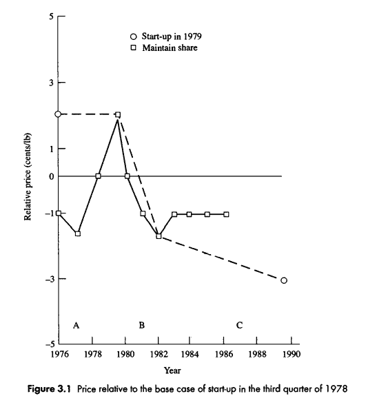
Beginning in 1972, Du Pont received a ‘large number’ of enquiries about licensing, particularly from National Lead [CX 33C]. But Du Pont seemed to be aware of the implications of licensing for the pattern of capacity expansion in the industry (section 1.4.) and rejected domestic requests without even calculating the royalties that might be generated.
As predicted, overseas licensing presented a different picture. No requests for licences from European producers were entertained, presumably because of Du Pont’s interest in competing directly in the West European titanium dioxide market. But Du Pont carefully explored licence applications from countries outside its zone of interest – Brazil, China, Japan, and the USSR. The Japanese proposal advanced to the negotiating stage but was shelved in autumn 1977 because of weak demand [CX $180 \mathrm{E}]$
The remedy proposed by the FTC in the antitrust case that it brought against Du Pont in 1978 also agrees with our analysis. The FTC’s appeal brief [p. 65] notes that: Royalty-free licensing would ‘break the chain’ of this pre-emptive process by immediately placing competitors in a position of cost parity with Du Pont . . Licensing with royalty fees would not be nearly as effective in upsetting the Du Pont ‘growth strategy’, since the effect of requiring royalty payments would be to maintain the Du Pont cost advantage over time. Competitors would continue to be at a cost disadvantage by the amount of royalty payment.
经济代写|产业经济学代写Industrial Economics代考|The devolution of declining industries
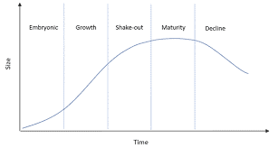
Models of dynamic competition generally take a rosy view of time: markets expand; better technologies become available; information improves. In this preoccupation with time as an engine of progress, environments in which time is an agent of regress have been shunted aside. Yet, declining industries form an important part of developed economies: more than 10 per cent of the United States’ 1977 manufacturing output was accounted for by industries whose real output had shrunk over the 1967-77 period.
In declining industries the important competitive moves pertain to disinvestment rather than investment. An industry facing decline must reduce its capacity in order to remain profitable. Capacity reduction, however, is a public good that must be provided privately. ${ }^{2}$ Each firm would like its competitors to shoulder the reduction: a firm may even maintain excess capacity – and sustain losses – in order to force competitors to withdraw sooner. The question arises: Who gives in first?
The timing game in a declining industry is therefore a war of attrition rather than a race to pre-empt. In the original model of the war of attrition (Maynard Smith, 1974), each competitor chooses between continuing to ‘fight’ at a pre-specified level of intensity or conceding; the competitor that hangs in the longest wins the prize. Ghemawat and Nalebuff (1985) applied this model, with its dichotomous choice, to declining industries by restricting production to be an all-or-nothing decision for each firm. This chapter, in sharp contrast, allows firms greater strategic flexibility by letting them continuously adjust their capacities as demand declines.
A large majority of economists – in my personal experience – think that if sellers announce, post or publish their (non-collusive) prices, they therefore use Bertrand strategies and thereby reveal that the Bertrand model is the appropriate one to use. Some even go as far as to argue that the Bertrand model has descriptive value. In my opinion, this reasoning is mistaken and results from a misunderstanding of the Cournot model. I shall indeed argue that it makes perfect sense to use Cournot strategies to explain real-world pricing.
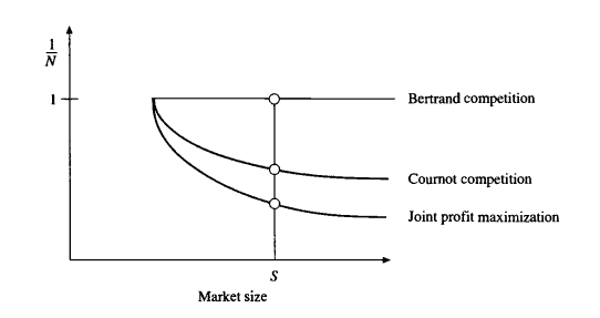
Let us have a closer look at Sutton’s example of a Cournot subgame (presented above in section 1.2). Market demand is $X=S / p$. There are $N$ identical firms, selling a homogeneous good, with profit function $$ \Pi_{i}=(p-c) x_{i} $$ where $p=S / X$. Let $X=X_{-i}+x_{i}$, where $X_{-i}$ is the sum of the outputs of all $i$ ‘s rivals. Then this profit function becomes $$ \Pi_{i}=\left(\frac{S}{X_{-i}+x_{i}}-c\right) x_{i} $$ and $$ \frac{\partial \Pi_{i}}{\partial x_{i}}=\frac{-S x_{i}}{\left(X_{-i}+x_{i}\right)^{2}}+\frac{S}{X_{-i}+x_{i}}-c=0 $$ are the first-order conditions. Because of the symmetry assumption, $x_{i}=x$ for all $i$ and these conditions become $$ \frac{-S x}{(N x)^{2}}+\frac{S}{N x}-c=0 $$ or $$ \frac{S(N-1)}{N^{2} x}=c $$ or $$ x=\frac{S}{c} \cdot \frac{N-1}{N^{2}} $$ implying $$ X=N x=\frac{S(N-1)}{c N} . $$
Before tackling their collusive aspect, I want to describe the functioning of a few pricing schemes that are frequently observed.
The Monopolies and Mergers Commission noted in its 1986 report on white salt that over the period under investigation the price of the two UK producers followed a pattern of ‘parallel pricing’. Every time there was a price change, one of the firms announced it while the other firm followed within a couple of weeks with an identical change. You might expect the bigger of the two firms to have been the price leader, but that was not the case: the smaller firm led eight times and the bigger firm led only five times. Notice that whoever took the initiative for a price change, informed the competitor a month in advance, and the latter would then inform the leader of a proposed identical change within that month. This is perhaps the most straightforward example of a pricing scheme as defined by d’Aspremont $e t$ al. (1991). There being only two firms and one taking over the price of the other, there is no need, really, to compute an average price. But the logic is the same: price signals, that is, announced prices are turned into one single price valid for all competitors.
The theoretical underpinning of the experiment on parallel pricing conducted by Harstad, Martin, and Normann (see chapter 6) is taken from MacLeod (1985), who supposes that $n$ firms follow a custom (called a ‘social convention’) which is to react to an announcement of a price change (by any competitor) according to an alignment rule. This rule says that firm $j$ should adopt price changes equal to those announced by $i$, whoever $i$ is. MacLeod applies this rule to differentiated as well as homogeneous goods, while d’Aspremont et al. (1991) consider only the original Cournot case of a homogeneous good, for which the producers must charge the same price in equilibrium. That is why the experiment is based on the assumption that the experimental subjects sell differentiated commodities.
MacLeod imagines the following strategy: (1) when a price increase is announced by a competitor, follow it if it is profitable to do so and if the others do the same; otherwise, do not change your price; (2) when a price decrease is announced by a competitor, follow it as long as it does not lead to prices lower than the prices that would obtain in a static non-collusive Nash equilibrium; (3) if any rival firm does not behave according to (1) and (2), announce the static non-cooperative Nash equilibrium price. Then there exists a non-cooperative equilibrium with prices higher than the noncollusive Nash prices but lower than those which would maximize the joint profit.
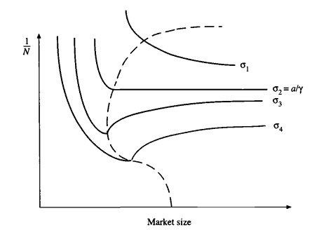
In Sutton’s terminology, endogenous sunk costs are those incurred with a view to enhancing consumers’ willingness-to-pay for a specific firm’s product. Implicit is the assumption that there are quality differences (or vertical differentiation) which the firms want to advertise or develop. So these costs are (mainly) advertising and R\&D costs. They increase with $u$, an index of perceived quality. On the consumers’ side, their willingness-to-pay is a non-decreasing function of $u$. Markets with these characteristics are what Schmalensee calls type II markets in chapter $2 .$
The natural thing to do is to take the two-stage game discussed above and insert an intermediate stage in which the firms that decided to enter (at cost $\sigma)$ in the first stage choose a value of $u$ (and therefore an advertising level or an R\&D effort) at a sunk cost $A(u)$ to be added to $\sigma$. In the third stage, then, the vector $\left{u_{i}\right}$ is given and firms compete (à la Cournot for example).
If advertising leads to sufficient increases in demand, then firms will increase their advertising costs $A(u)$ and thus increase total sunk costs $\sigma+A(u)$. Such an escalation of costs raises the equilibrium level of total sunk costs, which has now become endogenous. The end result is that there will not be room in the market for more and more firms as market size increases: market structure does not become more and more fragmented as $S$ increases, in sharp contradiction with type I markets.
All this hinges on the degree of demand responsiveness faced by the individual firms to increases in their advertising or $\mathrm{R} \& \mathrm{D}$ outlays or, in terms of costs, on the returns to these outlays. Sutton (1991, chapter 3 ) uses the convenient specification $$ A(u)=\frac{a}{\gamma}\left(u^{\gamma}-1\right), \quad \gamma>1 . $$ Putting $u=1$, we have $A(1)=0$ and $A^{\prime}(1)=a$. So a small initial outlay at $u=1$ produces a return corresponding to an expense $a$, which is the cost per message. On the other hand, a higher $\gamma$ implies more rapidly diminishing returns. The total fixed outlays function (which can thus be interpreted as the advertising response function) is then $$ \sigma+\frac{a}{\gamma}\left(u^{\gamma}-1\right) . $$
经济代写|产业经济学代写Industrial Economics代考|Dynamics of market expansion and contraction
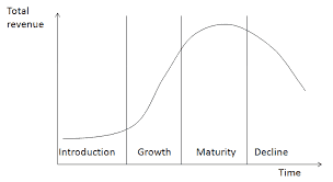
Chapters 3,4 , and 5 look into the dynamics of how market structure changes over time. The two preceding chapters showed how to determine the equilibrium number of firms $N^{}$. Now the problem is to figure out how $N$ is going to be increased when $N}$, for example when market demand is expanding and the potential producers have come to the conclusion that there is room for additional capacity. The alternative problem is to take the case of a contracting industry in which the producers have come to the conclusion that $N>N^{*}$ and to ask how the industry’s capacity is going to be reduced.
Both cases will be studied with the help of a so-called ‘timing’ game, that is, a game in which the players have to decide at what point in time they will do something. In the case of two players, they have to decide for example who will be first to make an announcement, to decide, to start producing or whatever. Our problem is: which firm will be first to invest in new capacity when demand expands and to close down or divest when demand contracts over time.
In chapter 3 , Ghemawat tells the story of Du Pont’s capacity expansion strategy in the US titanium dioxide industry and shows that it accords with the predictions of a timing game between two firms. Firm 1’s cost of constructing a new plant is lower than firm 2’s. These two firms are participating in a public auction ${ }^{6}$ in which they alternate in making bids about the dates at which they are willing to add capacity between time 0 and time $T$. One firm makes the first bid promising to add new capacity at time $t_{j}^{}$. If the other firm does not announce an earlier date before the end of the auction, that’s it. Alternatively, the other firm can announce that it will invest earlier in period $t_{j}^{}-s$, and thus ‘undercut’ the previous bid. This undercutting goes on as long as the resulting additional profit covers the cost of adding capacity. This profit is the present value of the profits that will be made as of the point in time at which the undercutter would add capacity if he were not undercut himself. Who will be the first to stop this bidding? The first player for which this profit is smaller than the cost of adding capacity (discounted to the present). This must be firm 2: the firm with higher capacity costs will be the first to stop bidding. Consequently, the low-cost firm will find it profitable to pre-empt the others in adding new capacity.
经济代写|产业经济学代写Industrial Economics代考|A two-stage game
Why suppose that this game has two stages? Why not suppose that the investments in setting up the equilibrium number of firms and the degree of competition are determined in a one-stage (‘one-shot’) game? The formulation of this question is possibly a bit confusing, in that it may suggest that the two-stage game is solved in two successive steps. So let me emphasize right from the start that the players of such a game solve its successive ‘subgames’ or steps before the game is actually started, as is the case with a one-shot game. (We shall see a bit later how the solution is found.)
The advantage, then, of distinguishing two stages is to disentangle the long-run and the short-run aspects of the problem without separating them. The first step, in which the investments or disinvestments (by entry into or by exit from the industry) are decided, is the long-run aspect of the problem. The second step, in which the profits that motivate the entries or the exits are determined, is the short-run aspect. The latter determines the former. But the former is ‘long-run’, since it is more difficult to change an investment decision than to change a price.
Since my undergraduate days, I have struggled with the distinction between the short run and the long run, which I encountered for the first time in Alfred Marshall’s Principles (1952, book V, chapter V, section 6). I quote:
To sum up then as regards short periods. The supply of specialized skill and ability, of suitable machinery and other material capital, and of the appropriate industrial organization has not time to be fully adapted to demand; but the producers have to adjust their supply to the demand as best they can with the appliances already at their disposal … In long periods on the other hand all investments of capital and effort in providing the material plant and the organization of a business, and in acquiring trade knowledge and specialized ability, have to be adjusted to the incomes which are expected to be earned by them: and the estimates of these incomes therefore directly govern supply.
Salt is a homogeneous commodity. So there is no point in organizing advertising campaigns to promote a particular brand nor is there in investing in $\mathrm{R} \& \mathrm{D}$ outlays to improve the quality of salt. In the absence of fixed costs for advertising and $R \& D$, the only fixed costs salt producers have to care about are the costs of setting up their plant. These costs $(\sigma)$ are exogenously given to them and cannot be recovered: they are sunk costs and therefore play no role in the day-to-day pricing policy.
To be more precise, $\sigma$ is the cost of acquiring a single plant of minimum efficient scale, net of resale value. In the first stage of the game, the entry decision is taken at this cost $\sigma$, which is treated as a fixed parameter in the second stage (so that prices do not depend directly on it). To justify entry, $\sigma$ must be recovered ex post, so entry decisions depend on the interplay between $\sigma$ and the intensity of competition. If competition turns out to be too intensive, then some existing plants have to be closed. (To make sure that the second-stage equilibrium prices are compatible with $\sigma$ and the corresponding market structure, the game is solved backwards as explained above. However, once the game is actually played and circumstances change, inconsistency may indeed arise and lead to a restructuring of the industry.)
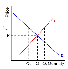
Sutton (1991, chapter 2) constructs the following example. Suppose market demand can be specified as $X=S / p$ where $X$ is the total quantity of salt demanded and $p$ is its price, so that $S$ is the total expenditure on salt. $S$ can thus be interpreted as the size of the market, while the price elasticity is supposed to be $-1$. (This specification has the advantage that we can make the market for salt grow or decline by simply letting the parameter $S$ grow or decline.) Suppose also that there is a price $p_{0}$ above which sales are zero.
经济代写|产业经济学代写Industrial Economics代考|Continue to Deepen Supply-Side Reform and Stimulate New Vitality of Industrial Growth
The supply-side reform’s emphasis on decisive roles of market in resource allocation aims to release new demands and create new supplies; on the one hand, market is supposed to release overcapacity and create new economic growth points, and on the other, the use is made of innovation to form effective supplies with higher quality and stimulate new demands. The supply-side reform is a specific remedy for the currently existing economic issues in China, a new method for China’s economic reform and an effective action to vitalize industrial growth. Firstly, we need to focus on release of excess capacity and elimination of “zombie” enterprises. The existing excess capacity, “zombie” and loss-making enterprises and low-efficiency or even inefficient assets are consuming huge quantity of resources and hinder transformation and upgrading of industrial structure. The Central Economic Working Conference stated expressly that top priority of supply-side structural reform in 2016 would be given to active and prudent dissolution of excess capacity and release of valuable resource elements from enterprises featuring severely excess capacity and limited space for growth and the “zombie” enterprises so as to improve effective supply and create new productivity by straightening out the supply side. To dissolve excess capacity, the Central Government, local government, authorities and enterprises must exercise strict control over incremental productive capacity. In particular, the local government is not supposed to increase investment blindly for local economic development or follow the suit simply because of huge potential in emerging industrials; instead, it should solve this problem at its source. The existing excess productive capacities may be dissolved by carrying out structural optimization or adjustment, promoting enterprise reorganization and M\&A, improving inventory warning mechanism and perform real-time monitoring over change in business inventories. Further solutions include: creating external demands and encouraging “go out” of China’s industrial capital to promote capacity output under the opportunity of the Belt and Road Initiative, accelerating reform of liberalization of production elements, breaking the government-led distribution mode of land and resources, giving full play to the regulating roles of market mechanism, and guiding allocation of capital and labor in all industrial sectors so as to dissolve excess capacity. As excess capacity is a systematic and long-term issue requiring both short-term administrative intervention and long-term governance according to the law, we need to improve the system of policy, laws and regulations for dissolution of excess capacity, and give full play to fiscal, financial and tax roles in the de-capacity process; accelerate consolidation, reorganization or bankruptcy of “zombie” enterprises or low-efficiency and inefficient assets, and make reasonable relocation of personnel and disposal of assets; actively guide upstream and downstream industrial organizations of the “zombie” enterprises to transform into high value added segments, or accept merging and reorganization of competitive industrial enterprises; and perfect the delisting mechanism of “zombie” enterprises to make adjustment and optimization of industrial structure, providing that the ecological equilibrium of these industrial organizations are maintained.
经济代写|产业经济学代写Industrial Economics代考|Expand Effective Demands and Further Exploit
Firstly, we need to make endeavors to promote supply-side reform, but it does not necessarily mean the quit of demand management; instead, implementation of the supply-side reform requires appropriate enlargement of aggregate demands; the supply-side reform and the demand management should promote and cooperate with each other. Since 2015 , obstructions have emerged in economic growth measures through expansion of investment and net export volume. The stabilizing and rising consumer goods market is unable to drive industrial growth, but the explosion of various emerging industries due to implementation of the innovation-driven strategy has brought about new possibilities for consumption and investment; as a result, the scale effect was replaced by consumption upgrading and investment efficiency in promoting industrial growth. In addition, the implementation of various regional strategies has provided unprecedented demand space for consumption and trade. In the second quarter of 2016 , more effective demands were exploited to promote industrial growth.
Secondly, we need to expand and upgrade consumption. On the one hand, we should focus on development of new technologies and new products, encourage innovation of commercial forms, create new demands by means of new supply, and direct consumers towards intelligent, green and healthy consumption. As the “imitative” consumption period comes to an end, individualized and diversified demand has become the mainstream consumption pattern; therefore, in addition to effort in new commercial forms, we need to make efforts on improvement product quality and grade to accommodate consumers’ individualized demands of products, and push consumption towards some new industries. On the other hand, we need to expand consumers’ demands by virtue of inter-regional collaboration strategies. As China’s economy develops, the consumption potentialities in central and western regions have been exploited to some extent. The current inter-regional collaboration strategy plays an important role in promoting consumption in the underdeveloped central and western regions. The “Yangtze River Economic Belt” is a significant action of China’s combination of regional coordination and opening up in the new period. This is an unprecedented policy that links together the eastern, central and western regions, and also a solid step to promote construction of inland economic belts. The western region of China is covered by the Belt and Road Initiative while the developed eastern region will take active part in the strategy by economic ties with central and western regions, and will promote inter-regional interactions through market force. All these will further exploit the consumption potentialities in the central and western regions. Meanwhile, “people foremost” is core to the new-type urbanization; more and more production factors such as rural population, information, capital and technologies that are flooding into cities will generate huge aggregation effect and scale effect in these cities to achieve better development of production factors market, especially the labor market; besides, rural laborers will get better paid in cities and will also improve incomes of urban residents and promote upgrading of consumption structure. Therefore, urbanization is an important means to expand consumption and promote consumption upgrading while the construction of the “Beijing-Tianjin-Hebei integration” and “Yangtze River Economic Belt” provides infinite opportunity for new-type urbanization. The inter-regional connection of public services, social insurance system and transportation will become the main market for future urbanization. To stimulate consumption, we need to make the best of inter-regional collaborative strategy to drive urbanization in the central and western regions; besides, we need to take active measures to optimize consumption environment, standardize market competition to facilitate transition of market competition from quantitative expansion and price competition to quality and differentiation competition, promote service-oriented development of manufacturing enterprises, protect consumers’ rights and interests, accelerate infrastructure construction in the field of consumer goods, and implement the “broadband China” strategy.
经济代写|产业经济学代写Industrial Economics代考|International Industries in the First Half of 2016
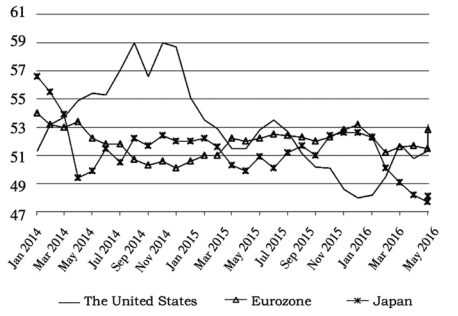
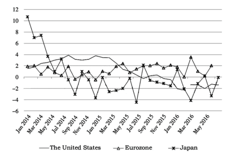
In the first half of 2016 , the world economy was still subject to a deep adjustment period after the financial crisis. Global manufacturing PMI index dropped from $50.1 \%$ in April to $50 \%$ in May 2016 . The industrial economics of major economies recovered slowly in a zigzag way and unevenly in main countries and regions, indicated significant uncertainty in industrial economics operation. In general, developed economies recovered faster than emerging economies did.
A weak recovery continued in developed countries, such as European countries and the United States. The American economy operated fairly well. Due to trade and government investment in consumption that offset slump in consumption, the year-on-year growth rate of American economy was modified to rise by $1.1 \%$, higher than the desired value and the last modified value. The American people’s confidence in economy was enhanced by the constantly recovering labor market, the higher employment rate and lower price index. The bounce-off of consumer spending in the second quarter will further promote American GDP growth. In addition, the American industrial production improved markedly. The overall production index (seasonally adjusted) entered year-on-year positive growth status, and the manufacturing PMI has climbed above the threshold since March 2016 , which kept ascending on a monthly basis in the first half year and hit a new high in June, so its manufacturing industry was expected to flourish; due to external environment’s influence, however, the American trade volume remained in sharp fluctuations, for which there was still large space for improvement. The Eurozone economy recovered slowly, with first quarter’s GDP growth rate higher than was expected. The Eurozone industrial production also recovered persistently. The manufacturing PMI in June was the highest this year, which indicated a recovering trend of Eurozone industry. Currently, the inflation pressure was slightly alleviated and generally better than market expectation, and the inflation that had lasted for four months eventually carne to an end in June. Eurozone saw a good trend of employment as the unemployment rates kept descending; due to British referendum on departure from the EU and its external environment, however, the Eurozone trade was not as optimistic as expected. Japan suffered a slow economic recovery,
regardless of its first quarter’s GDP growth rate higher than was expected. Other data indicated that Japanese economy remains flat and that continual fluctuations occurred in its industrial output, e.g. PMI in March stayed below the threshold, inflation risk remained and import/export trade volume kept shrinking.
Among major emerging economies, Brazil’s economy and industrial production continued shrinking, but the shrinking amplitude slowed down dramatically; despite a slight decline in the second quarter, Brazil’s PMI remained below the threshold in the first half of 2016 , with a rising unemployment rate and inflation. In the first quarter, South Africa’s economic growth rate went down significantly; the growth rate of industrial production fluctuated drastically; though the PMI began recovering up to the threshold in March, there was still uncertainty in its economic recovery as its inflation deteriorated and foreign trade fluctuated obviously. In comparison, India’s economy recovered more steadily, regardless of its sluggish industrial growth. In the first quarter of 2016 , India’s GDP grew $7.95 \%$ year on year, higher than the average of all quarters in 2015 , indicating a better recovering trend of India’s economy. Since the year of 2016 , India’s PMI maintained above the threshold; the decreasing amplitude of its foreign trade kept going down and improving steadily. Due to the declining international oil price, Russia’s economy continued with the downturn; industrial production remained sluggish, regardless of a slightly positive turnabout. In the first half of 2016 , Russia’s PMI basically remained below the threshold; the unemployment rate went up somewhat, but the inflation went down markedly and foreign trade improved to some extent. It was clear that as compared with developed economies, major emerging economies were faced with a more difficult problem in economic recovery. In the first half of 2016 , the general economic situation of developed economies seemed much better than aforesaid emerging economies.
经济代写|产业经济学代写Industrial Economics代考|Growth forecast and scenario analysis of industrial economics
With the current technological level, China’s industrial economics will be highly likely to maintain a slow-down growth rate from the second half of 2016 to the first half of 2017 , providing the current monetary and fiscal policies remain unchanged. According to the model prediction, the growth rate of China’s industrial economics will reduce to $5.7 \%$ at the end of 2016 and to $5.6 \%$ in June 2017 . Under the influence of moving holidays, obvious fluctuations will occur in industrial growth in January and February 2017 ; in remaining months of 2017 , the industrial economics will operate smoothly.
Benchmark: The quantities and qualities of labor force remain unchanged; the fixed asset investment maintain current development trend; the technical level remains unchanged; and the fiscal and monetary policies remain unchanged.
Scenario 1: The quantities and qualities of labor force remain unchanged; the fixed asset investment maintain current development trend; the technical level remains unchanged; and the fiscal and monetary policy strength is $20 \%$ lower than the current level.
Scenario 2: The quantities and qualities of labor force remain unchanged; the fixed asset investment maintain current development trend; the technical level remains unchanged; and the fiscal and monetary policy strength increases $20 \%$ over the current level.
经济代写|产业经济学代写Industrial Economics代考|Qunhui Huang and Hangyan Zhang
With implementation of a series of policies including the supple-side structural reform, the national economy operated quite well and stabilized in slow growth and slow recovery in the first half of 2016 . However, the recovery seems not so optimistic in the pessimistic context of the international situation that might complicate and intensify China’s industrial economy and might lead to heavier downturn pressure on economic operation in the second half of 2016 as a number of contradictions and risks stand out. In this case, we need to seize the new normal opportunity for economic development, steady growth by taking effective measures against various risks and challenges, promote reform and transformation, break institutional barriers and combine long-term policies with short-term ones, macro policies with micro ones and supply management with demand management so as to pave the way for healthy development of China’s industrial economics.
经济代写|产业经济学代写Industrial Economics代考|Focus on Steady Growth and Maintain Relative
Sharp fluctuations in economic growth are usually traceable back to sharp fluctuations in macro policies. As China’s industrial economics are currently “stabilizing in slow growth”, sharp fluctuations in macro policies should be avoided as taboos. In the first year of the “13th Five-Year Plan” $(2016-20)$, we need to maintain relative stability and continuity of macro policies, minimize frequent short-term macroeconomic control, deepen the concept of “interval control”, give play to the decisive roles of resource allocation in market and shift strategic focus to reform and adjustment of economic structure so that macro policies are authentic in promoting steady growth.
Firstly, we need to stabilize and avoid sharp fluctuations in real estate market. Such actions will be of great importance to economic growth and social stability. During the supply-side reform, de-stocking policies might be most intensive in real estate market; in just two dozen days since February 2016, five bombshell measures were issued by more than ten ministries and committees including the Central Bank of China and National Development and Reform Commission (NDRC), almost one real estate policy being issued per week. In such a context, the government should be active to direct and guide the expectations and behaviors of commercial banks and social public by means of various policy tools to prevent against sharp fluctuations in real estate market and insure stable, healthy development of the real estate market.
Then, we need to continue with proactive fiscal policy and steady monetary policy. Under the pressure of continuous economic downturn, we will implement proactive fiscal policy for tax abatement and increase of social security expenditure, provide support for enterprises in technical transformation and innovation investment and give play to the leading role of governmental investment, guide funds to flow into fields that may generate higher investment efficiency, guarantee implementation of state-approved projects, increase expenditure in unemployment insurance and low-income population, maintain social stability, and create a macro environment to the benefit of structural adjustment, exercise steady monetary policy, duly cut down on interest and reserve and bring down enterprises’ financing cost pursuant to economic recovery; in addition, relevant authorities should delivery policy signals in time to market so as to stabilize expectation and confidence on the stock market.
Finally, we need to renovate the methods of macroeconomic regulation and control, strengthen interval control and opportunistic control, make the best of policy tools such as industry, investment and price as well as the fiscal and monetary policies, and take measures for structural reform and especially for supply-side structural reform to prevent all risks and create a favorable environment for economic development.
经济代写|产业经济学代写Industrial Economics代考|Debt risks accumulated to pin down industrial operation
Local debt risk remains high. During economic deceleration, the fiscal revenue growth will slow down and the expenditure will rise moderately under the influence of economic fundamentals, enlarging the scale of deficit and debt. Furthermore, the fact that local governments may execute debt financing on various financing platforms to maintain goals of local economic and social development and to accelerate infrastructure construction will initiate a new mode to stimulate economic growth by governments’ leveraging investment. When the government no long provides any guarantee for these debts, some of the debts will be transferred by financing platforms to debts payable by the government; as a result, the debts payable by the local government will increase. According to the results of national debt audit at the end of 2015, RMB $1.9$ trillion debts payable by the government fell due in 2015 . Excessive debt ratio of the local government will put local government under heavy pressure to discharge debts and will also easily lead to crisis of local government debts; in addition, due to different rates of local economic growth and different debt burden of provinces, it is likely to incur local debt crisis. Excessive local government debts may also lead to risk of local government’s bankruptcy and place strict restrictions on local government’s further financing and on continuous investment in infrastructure construction and thus compromise the growth of industrial economics.
Potential risk in industrial sectors remains high. In May 2016, the debt-to-asset ratio of industrial enterprises above designated size was $56.8 \%, 0.6$ percentage point higher than December 2015 , and the leverage ratio reached up to $131 \%$, which increased the operating risk of industrial sectors. It is noted that the excessively high leverage ratio of Chinese enterprises was questioned as the leverage ratio of foreign enterprises maintained at around $70 \%$. In effect, the leverage ratio of Chinese enterprises has been extremely high for many years, for it was closely related to Chinese economic reality: (i) high saving rate that means relatively adequate supply of capitals in China, and (ii) high leverage that results from two realistic bases – relatively lagging development of China’s capital market and credit financing used as the main financing channel by China’s industrial sectors. However, these two bases are slowly collapsing as the consumer savings declines and the capital market expands and plays more financing functions. In recent years, the de-leverage ratio of industrial enterprises has paced up, reducing from $178 \%$ at the beginning of 1998 to $128 \%$ at the end of December 2015 . The current uptrend of leverage has no realistic base. Furthermore, the local government’s debt risks are constantly discharged. China as a whole suffers a very high debt ratio, so the increasing leverage will intensify the risk pressure.
经济代写|产业经济学代写Industrial Economics代考|Prediction of Industrial Growth Trend
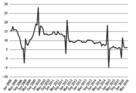
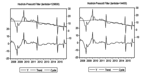
HP filtering method adopted in this report separates the growth trend of industrial value added year on year from cyclical factors to analyze roles of different factors in industrial value added. According to the results, the growth rate of industrial economics has slowed down since the year of 2010 ; the slowing growth rate has continued in the first half of 2016 but the decreasing amplitude was narrowing; and it is predicted that the industrial growth will highly likely hit the bottom in the second half of 2016 (1) Data source and interpolation of missing values In this report, the value added year-on-year growth data of industries above designated size are used as observing indicators of industrial growth, with the samples ranging between January 2008 and June 2016 . Data are sourced from National Bureau of Statistics website. The industrial value added year-on-year growth rate is: (i) calculated by comparable prices, independent of price factors and free from price adjustment, and (ii) value added growth data of industries above designated size with January growth data missed, which needs interpolation. The traceability method is adopted in this report to interpolate data. Specific steps are as follows. Firstly, the monthly year-on-year growth rate data and the monthly accumulative growth rate data of industrial value added as well as the monthly actual data in 2005 of industrial value added ${ }^{2}$ are obtained from National Bureau of Statistics website. Secondly, the monthly industrial value actually added in 2005 is used to figure out the monthly accumulative growth rates of industrial value added in 2005 . Thirdly, the monthly accumulative industrial value added in 2005 and the monthly accumulative growth rates of industrial value added in 2006 are used to calculate the monthly accumulative industrial value added in 2006 , and by analogy get the monthly accumulative industrial value added from 2007 to 2016 with January data missed. Fourthly, the monthly industrial value actually added in 2005 and the monthly year-on-year growth rates of industrial value added in 2006 are used to figure out the monthly industrial value actually added in 2006 , and by analogy get the monthly industrial value actually added from 2007 to 2016 with January data missed. Fifthly, the industrial values actually added in January from 2006 to 2013 are obtained by the accumulative number in February of industrial value added from 2006 to 2016 with January data missed minus the actual industrial value added in February from 2006 to 2016 . Finally, all monthly data calculated above are used to directly get the missing January data about the monthly year-on-year growth rates of industrial value added (Fig. 2.5).
In order to separate the long-term trend factors from the cyclical (irregular) factors of industrial growth and obtain estimation of unobservable potential factors, either the moving average method or the frequency domain estimation method may be used for the original data of single time sequence; the filtering method has a unique advantage, i.e. simple, intuitive and easy for implementation, and can also avoid the problem caused by production function method, i.e. whether the product function can be stable in the economic transition period, and the problem caused by variable structure decomposition method, i.e. whether there exists the Phillips curve of conventional form in China. Therefore, the HP filtering method is adopted in this section to predict the growth trend of industrial economics.
The HP filtering de-trending method may regard economic operation as a certain combination of potential growth and short-term fluctuations and use metrological technology to decompose the actually output sequence into trend components and cyclical components; the former means potential output while the latter means output gap or fluctuation. For growth rate of industrial operation, the time sequence $y_{t}$ consists of industrial operation trend $g_{t}$ and industrial operation fluctuation $c_{t}$, namely: $$ y_{t}=g_{t}+c_{t} \quad t=1, \ldots T $$ Hodrick and Prescott $(1980,1997)^{3}$ designed HP filter by following the logarithm data moving average method. The filter can obtain a smooth sequence $g_{t}$ from the time sequence $y_{t}$, i.e. trend component, and $g_{t}$ is the solution to the formula below: $$ \operatorname{Min}\left{\sum_{t=1}^{T}\left(y_{t}-g_{t}\right)^{2}+\lambda \sum_{t=1}^{T}\left[\left(g_{t}-g_{t-1}\right)\left(g_{t}-g_{t-2}\right)\right]\right} $$ where, $\sum_{t=1}^{T}\left(y_{t}-g_{t}\right)^{2}$ represents fluctuations, $\sum_{t=1}^{T}\left[\left(g_{t}-g_{t-1}\right)\left(g_{t}-g_{t-2}\right)\right]$ represents trend, and $\lambda$ is smooth parameter with a positive value used to adjust proportions of fluctuation and trend. Selection of the smooth parameter $\lambda$ is an important problem in the HP filtering method. Different smooth parameters mean different filters that determine different fluctuating modes and smoothness. According to Hodrick and Prescott $(1980,1997)$, the value of smooth parameter is taken as 100 in processing annual data, as 1600 in processing quarterly data and as 14,400 in processing monthly data. According to Ravn and Uhlig (2002), ${ }^{4}$ the smooth parameter should be 4th power of the observed data frequency, i.e. $6.25$ for annual data, 1600 for quarterly data and 129,600 for monthly data. In this report, the data used are growth rates of industrial value added from January 2010 to September 2015, sourced from National Bureau of Statistics website. It is important to note that the missing data on growth rates of industrial value added in January on National Bureau of Statistics website are supplemented by point linear interpolation in this report. Above two types of filters are selected for use in this report: $\lambda=14,400$ and $\lambda=129,600$.
经济代写|产业经济学代写Industrial Economics代考|Factors Influencing Cyclical Variation of Industrial Economics
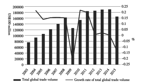
The cyclical fluctuation of industrial economics in the future will be subject to factors such as global economic recovery and changes in both national and international demands, and will therefore lead to cyclical variations of industrial economics. Various uncertainties will likely result in drastic fluctuation in the future industrial economics. (1) Sluggish global economy recovery and significant global trade slow down Since the year of 2008 , the growth of global international trade slowed down under the influence of financial crisis. Despite various incentive policies that simulated economic growth in 2010 and 2011 , the zero or even negative growth trend remained unchanged (see Fig. 2.4).
Economic differentiation continued in main economies of the world. The American economy saw a steady recovery and assumed a trend of slight growth. The European economy was recovering from European debt crisis and moving towards stabilization. The emerging economies witnessed obvious internal differentiation; India maintained a steady economic growth while Russia and Brazil suffered a negative growth. On the whole, the international economic situation has slightly improved, but the global economic growth still featured a too slow, fragile and unbalanced recovery. The US dollars appreciation and continuous decline of international oil price added more uncertainties to global financial markets and global economic recovery, such as intensification of global trade protection,expansion of exchange rate fluctuations, local economic upheaval and geopolitical tensions. Continuous changes of the world economic pattern have brought about huge risks and impact on China’s foreign trade and restriction on China’s external demands. In addition, the “Road and Belt” strategy involves many sensitive regions in Westem Asia and Eastern Europe, so the geopolitical tensions may have adverse effects on China’s overseas investment under the background of the Belt and Road Initiative and to some extent compromise industrial growth that should be stimulated by the Belt and Road Initiative.
In the international trade pattern, China’s industrial goods took up an increasingly high proportion. In 2003 , China’s industrial goods only took up $5.7 \%$ of global goods trade, but the proportion rose to $13.8 \%$ in 2015 , steadily increasing in more than ten years. Under the influence of shrinking global trade, China’s export growth rate slowed down and trade scale also withered, but China’s trade competitiveness witnessed a rising trend year by year; it is predicted that the rising trend of trade proportion will persist in $2016 .$
The comparative advantages of China’s industrial development are under various threats and interruptive risks. The competitive advantages of China’s industrial enterprises have over years depended on low-cost advantages based on low-level production factors. With the loss of demographic dividend, the rise of domestic factor cost, the intensification of resource and environment pressure and the expansion of economic scale, however, this low-cost advantage is diminishing little by little and the dividend in trade that uses low cost as the main competitiveness basically comes to an end. In addition, new advantages based on the high-level product factors can hardly be established in a short time and may interrupt competitive advantages, resulting in depression of industrial goods export, slowdown of economic growth rate and decline of enterprises’ international competitiveness. In contrast, some emerging economies, such as Southeast Asian and African countries, have lower labor cost than China, and the comparative advantages of labor force in these countries have come into market, tending to supersede China’s traditional advantages. In addition, the advanced manufacturing technology, information technology, biotechnology and energy technology spread quickly over the world and are widely used by developed countries to exploit potential markets and realize “backflow of manufacturing industry” and “reindustrialization”. The “backflow of manufacturing industry” and “reindustrialization” strategy of developed countries has enabled them to slow down overseas transfer of their manufacturing industries, especially the high-end manufacturing industries. The development of China’s hi-tech industries depends largely on the international market, so it will be more difficult for China to borrow technologies from developed countries; instead, China will rely on its financing cost, logistics cost and tax cost as well as the technological gap.
经济代写|产业经济学代写Industrial Economics代考|The effect of regional collaborative strategy
In March 2015, the Vision and Actions on Jointly Building the Silk Road Economic Belt and the 21 st-Century Maritime Silk Road was issued jointly by the National Development and Reform Commission (NDRC), Ministry of Foreign Affairs and Ministry of Commerce to promote construction of the Belt and Road Initiative. In April 2015, the Coordinated Development Program for Beijing-Tianjin-Hebei Region was adopted at the meeting of the Political Bureau of the CPC Central Committee. In October 2015, China’s 13th Five-Year Plan (2016-2020) on National Economic and Social Development, adopted at the Fifth Plenary Session of the 18th Communist Party of China $(\mathrm{CPC})$ Central Committee, proposed formation of the lengthwise and crosswise economic axial belt along the coast, the river and the line guided by the Belt and Road Initiative construction, Beijing-Tianjin-Hebei coordinated development and Yangtze River Economic Belt construction and based on the overall strategy of regional development, and formation of city clusters including the northeast region, the central plains region, the middle reaches of the Yangtze River region, the Chengdu-Chongqing region and the central Shaanxi region through prior development of such city clusters as Beijing-Tianjin-Hebei, the Yangtze River Delta and the Pearl River Delta.
The new demand space for China’s industrial development provided by the regional coordinated development strategy along with its policy effect has brought indefinite opportunities for China’s industrial development in the next year. Firstly, the strategy has driven the balanced development in these regions. For a long time, Chinese government’s focus on coastal regions for economic development has create many economic hot spots in the eastern regions with most advanced economic development and most sufficient utilization of funds; in contrast, the central and western regions, especially the western regions, saw a rather low fund utilization rate and a narrow extent of opening up to the outside world due to their location, which laid severe restrictions on economic development but indicated potential industrial demands. The formation of city clusters has led to industrial cluster effect and creation of an industrial development pattern in which the growth poles of Beijing and Shanghai will drive economic growth in surrounding provinces, favorable for optimization of urban spatial layout, coordination among industrial sectors and expansion of environmental capacity and ecological space; in particular, the “Yangtze River Economic Belt” covering 11 provinces and cities has linked together the eastern, central and western regions to form a coordinated development belt that allows interaction and cooperation among the eastern and western regions and drives economic development in the western region, has fundamentally changed the location conditions of the western regions as many provinces along the Belt and Road Initiative are located in West China, has broadened the opening-up extent in China’s northwestern and southwestern regions and provided opportunities for these regions to carry out foreign trade and foreign investment activities and achieve leap-forward development.