如果你也在 怎样代写信息论information theory这个学科遇到相关的难题，请随时右上角联系我们的24/7代写客服。

信息理论是对数字信息的量化、存储和通信的科学研究。该领域从根本上是由哈里-奈奎斯特和拉尔夫-哈特利在20世纪20年代以及克劳德-香农在20世纪40年代的作品所确立的。该领域处于概率论、统计学、计算机科学、统计力学、信息工程和电气工程的交叉点。

statistics-lab™ 为您的留学生涯保驾护航 在代写信息论information theory方面已经树立了自己的口碑, 保证靠谱, 高质且原创的统计Statistics代写服务。我们的专家在代写信息论information theory代写方面经验极为丰富，各种代写信息论information theory相关的作业也就用不着说。

我们提供的信息论information theory及其相关学科的代写，服务范围广, 其中包括但不限于:

• Statistical Inference 统计推断
• Statistical Computing 统计计算
• Advanced Probability Theory 高等概率论
• Advanced Mathematical Statistics 高等数理统计学
• (Generalized) Linear Models 广义线性模型
• Statistical Machine Learning 统计机器学习
• Longitudinal Data Analysis 纵向数据分析
• Foundations of Data Science 数据科学基础

数学代写|信息论作业代写information theory代考|Systems with Four Interacting Spins

In this and in the next few sections we study the MI among larger number of spins. As we have noted in Chap. 4 of Ben-Naim [1], there are several possible generalizations of the MI. In Chap. 4 of Ben-Naim [1] we discussed mainly two generalizations of the MI.

The first was referred to as the total MI denoted TI. This is defined for any number of random variables (or experiments) by:
$$
T I\left(X_1 ; \ldots ; X_n\right)=\sum p\left(x_1, \ldots x_n\right) \log g\left(x_1, \ldots, x_n\right)
$$
where $p\left(x_1, \ldots, x_n\right)$ is the probability of finding the event $\left{X_1=x_1, X_2=\right.$ $\left.x_2, \ldots X_n=x_n\right)$ and $g\left(x_1, \ldots, x_n\right)$ is the correlation function, defined by:
$$
g\left(x_1, \ldots, x_n\right)=\frac{P\left(x_1, \ldots, x_n\right)}{\prod_{i=1}^n P\left(x_i\right)}
$$
The second generalization was referred to as the conditional MI, and denoted $\mathrm{CI}$. There are several possible definitions of CI. Here, we use the one chosen by Matsuda [3]. This is not the most informative form of $\mathrm{CI}$, however, we use this particular one to compare our results with Matsuda’s results. This definition is:
$$
C I\left(X_1 ; \ldots ; X_n\right)=\sum_{k=1}^n(-1)^{k-1} \sum_{\left(i_1, \ldots, i_k\right)} H\left(X_1, \ldots X_n\right)
$$
Here, the sum on the right hand side of (3.43) is over-all possible sets of indices $\left(i_1, i_2, \ldots, i_k\right)$, with $: 1<i_1<i_2<\ldots i_k<k$.
As we have noted several times, this quantity may be negative.

数学代写|信息论作业代写information theory代考|Four-Spin Systems; Perfect Square

Figure 3.23 shows three possible arrangements of the four spins system: (a) is a regular square with equal edges. (b) is a parallelogram in which the distance between 1 and 3 is the same between 1 and 3 and (c) a rectangle with two short and two twice longer edges.

For the arrangement of Fig. 3.20a the total number of configurations is $2^4=16$. Again, we assign the value of $(+1)$ to the “up” and $(-1) \ldots$

In Sect. 4.10 of Ben-Naim [1] we presented some details about the various SMI, the pair and triplet MI, etc. Here, we proceed directly to discuss only the total MI and the conditional MI.

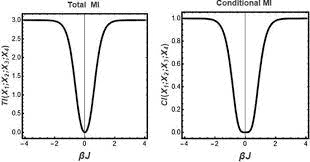
Figure 3.24 shows TI and $\mathrm{CI}$ for the square arrangement. For $\beta J=0$ (either $J=0$ or $T \rightarrow \infty$ ) there is no correlation between the spins. Hence, both TI and CI

are zero. For larger $\beta J$ (either positive or negative) the behavior is similar for both TI and CI.
For the TI, we have in this limit
$$
\begin{aligned}
T I\left(X_1 ; X_2 ; X_3 ; X_4\right) & =-H\left(X_1, X_2, X_3, X_4\right)+4 H\left(X_1\right) \
& =-1+4=3
\end{aligned}
$$
The reason for this result is clear for very strong interactions there are only two configurations for the four spins with equal probabilities. Iherefore, the SMI for the four spins is one, as well as for each individual spin.

Unlike the case of three spins for which the behavior of $\mathrm{CI}$ is different for positive and negative $\beta J$, here, we have the same behavior for both $\beta J \rightarrow \pm \infty$. The actual value is $\log _2 2=1$, which may be calculated from equation:

$$
\begin{aligned}
& C I\left(X_1 ; X_2 ; X_3 ; X_4\right)=4 H\left(X_1\right)-4 H\left(X_1, X_2\right) \
& \quad-2 H\left(X_1, X_3\right)+4 H\left(X_1, X_2, X_3\right)-H\left(X_1, X_2, X_3, X_4\right) \
& \quad \rightarrow 4-4-2+4-1=1
\end{aligned}
$$
Note that unlike the case of triangle we do not have frustration in this case. As we noted earlier Matsuda attributed the negative value of the $\mathrm{CI}$ to the frustration effect.

信息论代写

数学代写|信息论作业代写information theory代考|Systems with Four Interacting Spins

在本节和接下来的几节中，我们将研究大量自旋中的 MI。正如我们在第 1 章中提到的那样。Ben-Naim [1] 的第 4 节中， $M I$ 有几种可能的概括。在第一章 Ben-Naim [1] 的第 4 章我们主要讨论了 MI 的两个概 括。
第一个被称为总 $\mathrm{MI}$ ，表示为 $\mathrm{Tl}$ 。这是为任意数量的随机变量 (或实验) 定义的:
$$
T I\left(X_1 ; \ldots ; X_n\right)=\sum p\left(x_1, \ldots x_n\right) \log g\left(x_1, \ldots, x_n\right)
$$
andg\left(x_1, \dots, $\left.\mathrm{x} _\mathrm{n} \backslash \mathrm{right}\right)$ isthecorrelation function, de finedby :
$g\left(x_1, \ldots, x_n\right)=\frac{P\left(x_1, \ldots, x_n\right)}{\prod_{i=1}^n P\left(x_i\right)}$
Thesecondgeneralizationwasre ferredtoastheconditionalMI, anddenoted $\backslash$ mathrm ${\mathrm{Cl}}$ .ThereareseveralpossibledefinitionsofCI. Here, weusetheonechosenby Matsuda[3]. T Imathrm ${\mathrm{Cl}}$
, however, weusethisparticularonetocompareourresultswith Matsuda’sresults. Thisde $C I\left(X_1 ; \ldots ; X_n\right)=\sum_{k=1}^n(-1)^{k-1} \sum_{\left(i_1, \ldots, i_k\right)} H\left(X_1, \ldots X_n\right)$
Here, thesumontherighthandsideof $(3.43)$ isover – allpossiblesetsofindices $\backslash$ feft(i_1, i_2, \dots, i_klright), with: $1<i _1<i _2<1 /$ dots i_k $<k \$$ 。
正如我们多次提到的，这个数量可能是负数。

数学代写|信息论作业代写information theory代考|Four-Spin Systems; Perfect Square

图 3.23 显示了四自旋系统的三种可能排列: (a) 是一个具有相等边的规则正方形。(b) 是一个平行四边 形，其中 1 和 3 之间的距离在 1 和 3 之间是相同的，(c) 是一个具有两条短边和两条长两倍边的矩形。
对于图 3.20a 的布置，配置总数为 $2^4=16$. 同样，我们赋值 $(+1)$ 到“向上”和 $(-1) \ldots$
昆虫。在 Ben-Naim [1] 的 4.10 节中，我们介绍了各种 SMI、配对和三元组 MI 等的一些细节。这里，我 们直接只讨论总 $\mathrm{MI}$ 和条件 $\mathrm{MI}$ 。
图 3.24 显示了 $\mathrm{TI}$ 和CI对于正方形排列。为了 $\beta J=0$ (任何一个 $J=0$ 或者 $T \rightarrow \infty$ ) 自旋之间没有相 关性。因此， $\mathrm{TI}$ 和 $\mathrm{Cl}$
为零。对于较大的 $\beta J$ (正面或负面) $\mathrm{TI}$ 和 $\mathrm{Cl}$ 的行为相似。
对于 $\mathrm{TI}$ ，我们有这个限制
$$
T I\left(X_1 ; X_2 ; X_3 ; X_4\right)=-H\left(X_1, X_2, X_3, X_4\right)+4 H\left(X_1\right) \quad=-1+4=3
$$
这个结果的原因很明显，对于非常强的相互作用，四个自旋只有两种配置，概率相等。因此，四个旋转 的 SMI 是一个，每个单独的旋转也是如此。
与三个自旋的情况不同，其中的行为CI正负不同 $\beta J$ ，在这里，我们对两者都有相同的行为 $\beta J \rightarrow \pm \infty$. 实际值是 $\log _2 2=1$ ，可以从等式计算:
$$
C I\left(X_1 ; X_2 ; X_3 ; X_4\right)=4 H\left(X_1\right)-4 H\left(X_1, X_2\right) \quad-2 H\left(X_1, X_3\right)+4 H\left(X_1, X_2, X_3\right)
$$
请注意，与三角形的情况不同，我们在伩种情况下没有挫败感。正如我们之前提到的，松田将负值归因 于CI达到挫败感。

统计代写请认准statistics-lab™. statistics-lab™为您的留学生涯保驾护航。

金融工程代写

金融工程是使用数学技术来解决金融问题。金融工程使用计算机科学、统计学、经济学和应用数学领域的工具和知识来解决当前的金融问题，以及设计新的和创新的金融产品。

非参数统计代写

非参数统计指的是一种统计方法，其中不假设数据来自于由少数参数决定的规定模型；这种模型的例子包括正态分布模型和线性回归模型。

广义线性模型代考

广义线性模型（GLM）归属统计学领域，是一种应用灵活的线性回归模型。该模型允许因变量的偏差分布有除了正态分布之外的其它分布。

术语 广义线性模型（GLM）通常是指给定连续和/或分类预测因素的连续响应变量的常规线性回归模型。它包括多元线性回归，以及方差分析和方差分析（仅含固定效应）。

有限元方法代写

有限元方法（FEM）是一种流行的方法，用于数值解决工程和数学建模中出现的微分方程。典型的问题领域包括结构分析、传热、流体流动、质量运输和电磁势等传统领域。

有限元是一种通用的数值方法，用于解决两个或三个空间变量的偏微分方程（即一些边界值问题）。为了解决一个问题，有限元将一个大系统细分为更小、更简单的部分，称为有限元。这是通过在空间维度上的特定空间离散化来实现的，它是通过构建对象的网格来实现的：用于求解的数值域，它有有限数量的点。边界值问题的有限元方法表述最终导致一个代数方程组。该方法在域上对未知函数进行逼近。[1] 然后将模拟这些有限元的简单方程组合成一个更大的方程系统，以模拟整个问题。然后，有限元通过变化微积分使相关的误差函数最小化来逼近一个解决方案。

tatistics-lab作为专业的留学生服务机构，多年来已为美国、英国、加拿大、澳洲等留学热门地的学生提供专业的学术服务，包括但不限于Essay代写，Assignment代写，Dissertation代写，Report代写，小组作业代写，Proposal代写，Paper代写，Presentation代写，计算机作业代写，论文修改和润色，网课代做，exam代考等等。写作范围涵盖高中，本科，研究生等海外留学全阶段，辐射金融，经济学，会计学，审计学，管理学等全球99%专业科目。写作团队既有专业英语母语作者，也有海外名校硕博留学生，每位写作老师都拥有过硬的语言能力，专业的学科背景和学术写作经验。我们承诺100%原创，100%专业，100%准时，100%满意。

随机分析代写

随机微积分是数学的一个分支，对随机过程进行操作。它允许为随机过程的积分定义一个关于随机过程的一致的积分理论。这个领域是由日本数学家伊藤清在第二次世界大战期间创建并开始的。

时间序列分析代写

随机过程，是依赖于参数的一组随机变量的全体，参数通常是时间。 随机变量是随机现象的数量表现，其时间序列是一组按照时间发生先后顺序进行排列的数据点序列。通常一组时间序列的时间间隔为一恒定值（如1秒，5分钟，12小时，7天，1年），因此时间序列可以作为离散时间数据进行分析处理。研究时间序列数据的意义在于现实中，往往需要研究某个事物其随时间发展变化的规律。这就需要通过研究该事物过去发展的历史记录，以得到其自身发展的规律。

回归分析代写

多元回归分析渐进（Multiple Regression Analysis Asymptotics）属于计量经济学领域，主要是一种数学上的统计分析方法，可以分析复杂情况下各影响因素的数学关系，在自然科学、社会和经济学等多个领域内应用广泛。

MATLAB代写

MATLAB 是一种用于技术计算的高性能语言。它将计算、可视化和编程集成在一个易于使用的环境中，其中问题和解决方案以熟悉的数学符号表示。典型用途包括：数学和计算算法开发建模、仿真和原型制作数据分析、探索和可视化科学和工程图形应用程序开发，包括图形用户界面构建MATLAB 是一个交互式系统，其基本数据元素是一个不需要维度的数组。这使您可以解决许多技术计算问题，尤其是那些具有矩阵和向量公式的问题，而只需用 C 或 Fortran 等标量非交互式语言编写程序所需的时间的一小部分。MATLAB 名称代表矩阵实验室。MATLAB 最初的编写目的是提供对由 LINPACK 和 EISPACK 项目开发的矩阵软件的轻松访问，这两个项目共同代表了矩阵计算软件的最新技术。MATLAB 经过多年的发展，得到了许多用户的投入。在大学环境中，它是数学、工程和科学入门和高级课程的标准教学工具。在工业领域，MATLAB 是高效研究、开发和分析的首选工具。MATLAB 具有一系列称为工具箱的特定于应用程序的解决方案。对于大多数 MATLAB 用户来说非常重要，工具箱允许您学习和应用专业技术。工具箱是 MATLAB 函数（M 文件）的综合集合，可扩展 MATLAB 环境以解决特定类别的问题。可用工具箱的领域包括信号处理、控制系统、神经网络、模糊逻辑、小波、仿真等。

R语言代写	问卷设计与分析代写
PYTHON代写	回归分析与线性模型代写
MATLAB代写	方差分析与试验设计代写
STATA代写	机器学习/统计学习代写
SPSS代写	计量经济学代写
EVIEWS代写	时间序列分析代写
EXCEL代写	深度学习代写
SQL代写	各种数据建模与可视化代写

如果你也在 怎样代写信息论information theory这个学科遇到相关的难题，请随时右上角联系我们的24/7代写客服。

信息理论是对数字信息的量化、存储和通信的科学研究。该领域从根本上是由哈里-奈奎斯特和拉尔夫-哈特利在20世纪20年代以及克劳德-香农在20世纪40年代的作品所确立的。该领域处于概率论、统计学、计算机科学、统计力学、信息工程和电气工程的交叉点。

statistics-lab™ 为您的留学生涯保驾护航 在代写信息论information theory方面已经树立了自己的口碑, 保证靠谱, 高质且原创的统计Statistics代写服务。我们的专家在代写信息论information theory代写方面经验极为丰富，各种代写信息论information theory相关的作业也就用不着说。

我们提供的信息论information theory及其相关学科的代写，服务范围广, 其中包括但不限于:

• Statistical Inference 统计推断
• Statistical Computing 统计计算
• Advanced Probability Theory 高等概率论
• Advanced Mathematical Statistics 高等数理统计学
• (Generalized) Linear Models 广义线性模型
• Statistical Machine Learning 统计机器学习
• Longitudinal Data Analysis 纵向数据分析
• Foundations of Data Science 数据科学基础

数学代写|信息论作业代写information theory代考|The Three-Spin System with External Field

In this section we study the effect of an external field on the MI between the three spins in the triangular configuration. Since we did not specify the type of the dipoles we assume here that the interactions between any pair of spins is as in Eq. 3.39, below. In addition, we add an additional field $(f)$, which favors the “up” orientation of the spin. Thus, the total energy of the system is given by:
$$
\begin{aligned}
U\left(x_1, x_2, x_3\right)= & -J\left(x_1 \times x_2+x_1 \times x_3+x_2 \times x_2\right) \
& -f\left(x_1+x_2+x_3\right)
\end{aligned}
$$
All the probabilities for this system are calculated as before from Eq. 3.36. For the case $f=0$ (i.e. no external field) we have for $\beta J=1$, two energy levels; “all up” and “all down” with probability 0.474 , and four other higher energy levels with probability of 0.087 . The total MI, (TI) and the conditional MI (CI) are shown as a function of $\beta J$ in Fig. 3.16. $\left(\beta J\right.$ is simply $\frac{J}{k_B T}$ with $\left.k_B=1\right)$.
Note that in this case we have the limiting values of $\mathrm{CI}$ and $\mathrm{TI}$ as:
$$
\begin{aligned}
& \lim {\beta J \rightarrow-\infty} C I=-0.17, \lim {\beta J \rightarrow \infty} C I=1 \
& \lim {\beta J \rightarrow-\infty} T I=0.4, \quad \lim {\beta J \rightarrow \infty} T I=1 \
&
\end{aligned}
$$
Turning on a small external field, $\beta f=0.1$ has a negligible effect on either $\mathrm{CI}$ or TI, however there are now four, rather than two energy levels with corresponding probabilities:

For “all up” configuration Pr $=0.613$, but for the “all down” configuration $\operatorname{Pr}=0.336$. Also, the six configurations, which had equal probabilities in the case $\beta J=0$ are now split into two groups:
$$
\begin{gathered}
p(1,-1,1)=p(1,1,-1)=p(-1,1,1)=0.0092 \
p(1,-1,-1)=p(-1,-1,1)=p(-1,1,-1)=0.0075
\end{gathered}
$$
All these changes in the probabilities are understandable as the effect of the external field favors the “up” orientation of each of the spins.

数学代写|信息论作业代写information theory代考|The Three-Spin System with Different Geometries

We discuss here another example of a three-spin system but with changing the geometry of the configuration of the triangle. We fix the distance between the two spins $X_1$ and $X_2$, and change the distance of the third spin $X_3$ as shown in Fig. 3.20.
We choose the distance between $X_1$ and $X_2$ as unity $(d=1)$. The distance between $X_3$ and $X_1$ will be the same as the distance between $X_3$ and $X_2$ and will be denoted $d$ (in units of the distance between $X_1$ and $X_2$ ).

Figure 3.21 shows the total and the conditional MI for the distance $d=2$. The limiting values of $\mathrm{CI}$ and $\mathrm{TI}$ in this case are:
$$
\begin{aligned}
& \lim {\beta J \rightarrow-\infty} C I \approx 0 \lim {\beta J \rightarrow \infty} C I=1 \
& \lim {\beta J \rightarrow-\infty} T I=1 \lim {\beta J \rightarrow \infty} T I=2
\end{aligned}
$$

Note that for small and negative values of $\beta J$ the $\mathrm{CI}$ is negative and it approaches zero for $\beta J \rightarrow-\infty$.

Figure 3.22 shows the $\mathrm{CI}$ and TI for $d=10$. At this distance the interaction between $X_3$ and either $X_1$ or $X_2$ is almost zero. We do not expect any frustration in this system and we see that the $\mathrm{CI}$ is almost zero for the entire range of negative $\beta J$. The limiting values of both $\mathrm{CI}$ and $\mathrm{TI}$ at $\beta J \rightarrow \infty$ are the same as in the case of $d=2$, i.e. they are 1 and 2 , respectively.

Finally, we bring $X_3$ to a distance $d=0.5$, which means we have a linear arrangement of the three spins see Fig. 3.20. Note however, that unlike the linear case discussed in Sect. 3.8.3, where we had only nearest-neighbors interactions (between $X_1$ and $X_2$, and between $X_2$ and $X_3$ ), here we have interactions between the three pairs of spins. We leave this case as an exercise. Here, we note that the limiting values of $\mathrm{CI}$ at both limits $\beta J \perp \infty$ is one, and for $\mathrm{TI}$ it is 2 . One interesting aspect of $\mathrm{CI}$ is that for small negative $\beta J \approx-0.5$ we have a small negative value of CI. The reader is urged to ponder on the question whether we can say that this negative $\mathrm{CI}$ is due to “frustration,” and if it is why this effect disappears when $\beta J \rightarrow-\infty$.

信息论代写

数学代写|信息论作业代写information theory代考|The Three-Spin System with External Field

在本节中，我们研究了外场对三角形配置中三个自旋之间 MI 的影响。由于我们没有指定偶极子的类型， 我们在这里假设任何一对自旋之间的相互作用如方程式。 3.39 ，如下。此外，我们添加一个额外的字段 $(f)$ ，这有利于自旋的“向上”方向。因此，系统的总能量由下式给出：
$$
U\left(x_1, x_2, x_3\right)=-J\left(x_1 \times x_2+x_1 \times x_3+x_2 \times x_2\right) \quad-f\left(x_1+x_2+x_3\right)
$$
这个系统的所有概率都是从方程式计算的。3.36. 对于案例 $f=0$ (即没有外场) 我们有 $\beta J=1$, 两个能 级; “全部上升”和“全部下降”的概率为 0.474 ，以及其他四个更高的能量水平，概率为 0.087 。总 MI (TI) 和 条件 $\mathrm{MI}(\mathrm{Cl})$ 显示为函数 $\beta J$ 在图 3.16 中。 $\left(\beta J\right.$ 简直是 $\frac{J}{k_B T}$ 和 $\left.k_B=1\right)$.
请注意，在这种情况下，我们的极限值为CI和 $\mathrm{TI}$ 作为:
$$
\lim \beta J \rightarrow-\infty C I=-0.17, \lim \beta J \rightarrow \infty C I=1 \quad \lim \beta J \rightarrow-\infty T I=0.4, \quad \lim \beta J \rightarrow \infty
$$
打开一个小的外场， $\beta f=0.1$ 对两者的影响都可以忽略不计CI或 $\mathrm{TI}$ ，但是现在有四个，而不是两个具 有相应概率的能级：
对于“全部启动”配置 $\operatorname{Pr}=0.613$ ，但对于“全部关闭”配置 $P r=0.336$. 此外，在案例中具有相同概率的 六种配置 $\beta J=0$ 现在分为两组:
$$
p(1,-1,1)=p(1,1,-1)=p(-1,1,1)=0.0092 p(1,-1,-1)=p(-1,-1,1)=p(-1,1,-1)
$$
所有这些概率变化都是可以理解的，因为外部场的影响有利于每个自旋的“向上”方向。

数学代写|信息论作业代写information theory代考|The Three-Spin System with Different Geometries

我们在这里讨论另一个三自旋系统的例子，但改变了三角形构型的几何形状。我们固定两个自旋之间的 距离 $X_1$ 和 $X_2$ ，并改变第三次旋转的距离 $X_3$ 如图 3.20 所示。
我们选择之间的距离 $X_1$ 和 $X_2$ 作为统一体 $(d=1)$. 之间的距离 $X_3$ 和 $X_1$ 将与之间的距离相同 $X_3$ 和 $X_2$ 并将被表示 $d$ (以之间的距离为单位 $X_1$ 和 $X_2$ ).
图 3.21 显示了距离的总 $\mathrm{MI}$ 和条件 $\mathrm{Ml} I=2$. 的极限值CI和 TI在这种情况下是:
$$
\lim \beta J \rightarrow-\infty C I \approx 0 \lim \beta J \rightarrow \infty C I=1 \quad \lim \beta J \rightarrow-\infty T I=1 \lim \beta J \rightarrow \infty T I=2
$$
请注意，对于较小的负值 $\beta J$ 这 $\mathrm{CI}$ 是负的，它接近于零 $\beta J \rightarrow-\infty$.
图 3.22 显示了 $\mathrm{CI}$ 和德州仪器 $d=10$. 在这个距离之间的相互作用 $X_3$ 和 $X_1$ 或者 $X_2$ 几乎为零。我们不布 望这个系统有任何挫败感，我们看到CI在整个负值范围内几乎为零 $\beta J$. 两者的极限值CI和TI在 $\beta J \rightarrow \infty$ 与 $d=2$ ， 即它们分别是 1 和 2 。
最后，我们带来 $X_3$ 到远处 $d=0.5$ ，这意味着我们有三个自旋的线性排列，见图 3.20。但是请注意，这 与第 1 节中讨论的线性情况不同。3.8.3，我们只有最近邻交互 (之间 $X_1$ 和 $X_2$, 以及介于 $X_2$ 和 $X_3$ ）, 这 里我们有三对自旋之间的相互作用。我们把这个案例留作练习。在这里，我们注意到的极限值CI在两个 极限 $\beta J \perp \infty$ 是一，并且对于TI它是 2 。一个有趣的方面 $\mathrm{CI}$ 是小负 $\beta J \approx-0.5$ 我们有一个小的 CI负 值。敦促读者思考我们是否可以说这种否定的问题CI是由于“挫败感”，如果这就是为什么当 $\beta J \rightarrow-\infty$

统计代写请认准statistics-lab™. statistics-lab™为您的留学生涯保驾护航。

金融工程代写

金融工程是使用数学技术来解决金融问题。金融工程使用计算机科学、统计学、经济学和应用数学领域的工具和知识来解决当前的金融问题，以及设计新的和创新的金融产品。

非参数统计代写

非参数统计指的是一种统计方法，其中不假设数据来自于由少数参数决定的规定模型；这种模型的例子包括正态分布模型和线性回归模型。

广义线性模型代考

广义线性模型（GLM）归属统计学领域，是一种应用灵活的线性回归模型。该模型允许因变量的偏差分布有除了正态分布之外的其它分布。

术语 广义线性模型（GLM）通常是指给定连续和/或分类预测因素的连续响应变量的常规线性回归模型。它包括多元线性回归，以及方差分析和方差分析（仅含固定效应）。

有限元方法代写

有限元方法（FEM）是一种流行的方法，用于数值解决工程和数学建模中出现的微分方程。典型的问题领域包括结构分析、传热、流体流动、质量运输和电磁势等传统领域。

有限元是一种通用的数值方法，用于解决两个或三个空间变量的偏微分方程（即一些边界值问题）。为了解决一个问题，有限元将一个大系统细分为更小、更简单的部分，称为有限元。这是通过在空间维度上的特定空间离散化来实现的，它是通过构建对象的网格来实现的：用于求解的数值域，它有有限数量的点。边界值问题的有限元方法表述最终导致一个代数方程组。该方法在域上对未知函数进行逼近。[1] 然后将模拟这些有限元的简单方程组合成一个更大的方程系统，以模拟整个问题。然后，有限元通过变化微积分使相关的误差函数最小化来逼近一个解决方案。

tatistics-lab作为专业的留学生服务机构，多年来已为美国、英国、加拿大、澳洲等留学热门地的学生提供专业的学术服务，包括但不限于Essay代写，Assignment代写，Dissertation代写，Report代写，小组作业代写，Proposal代写，Paper代写，Presentation代写，计算机作业代写，论文修改和润色，网课代做，exam代考等等。写作范围涵盖高中，本科，研究生等海外留学全阶段，辐射金融，经济学，会计学，审计学，管理学等全球99%专业科目。写作团队既有专业英语母语作者，也有海外名校硕博留学生，每位写作老师都拥有过硬的语言能力，专业的学科背景和学术写作经验。我们承诺100%原创，100%专业，100%准时，100%满意。

随机分析代写

随机微积分是数学的一个分支，对随机过程进行操作。它允许为随机过程的积分定义一个关于随机过程的一致的积分理论。这个领域是由日本数学家伊藤清在第二次世界大战期间创建并开始的。

时间序列分析代写

随机过程，是依赖于参数的一组随机变量的全体，参数通常是时间。 随机变量是随机现象的数量表现，其时间序列是一组按照时间发生先后顺序进行排列的数据点序列。通常一组时间序列的时间间隔为一恒定值（如1秒，5分钟，12小时，7天，1年），因此时间序列可以作为离散时间数据进行分析处理。研究时间序列数据的意义在于现实中，往往需要研究某个事物其随时间发展变化的规律。这就需要通过研究该事物过去发展的历史记录，以得到其自身发展的规律。

回归分析代写

多元回归分析渐进（Multiple Regression Analysis Asymptotics）属于计量经济学领域，主要是一种数学上的统计分析方法，可以分析复杂情况下各影响因素的数学关系，在自然科学、社会和经济学等多个领域内应用广泛。

MATLAB代写

MATLAB 是一种用于技术计算的高性能语言。它将计算、可视化和编程集成在一个易于使用的环境中，其中问题和解决方案以熟悉的数学符号表示。典型用途包括：数学和计算算法开发建模、仿真和原型制作数据分析、探索和可视化科学和工程图形应用程序开发，包括图形用户界面构建MATLAB 是一个交互式系统，其基本数据元素是一个不需要维度的数组。这使您可以解决许多技术计算问题，尤其是那些具有矩阵和向量公式的问题，而只需用 C 或 Fortran 等标量非交互式语言编写程序所需的时间的一小部分。MATLAB 名称代表矩阵实验室。MATLAB 最初的编写目的是提供对由 LINPACK 和 EISPACK 项目开发的矩阵软件的轻松访问，这两个项目共同代表了矩阵计算软件的最新技术。MATLAB 经过多年的发展，得到了许多用户的投入。在大学环境中，它是数学、工程和科学入门和高级课程的标准教学工具。在工业领域，MATLAB 是高效研究、开发和分析的首选工具。MATLAB 具有一系列称为工具箱的特定于应用程序的解决方案。对于大多数 MATLAB 用户来说非常重要，工具箱允许您学习和应用专业技术。工具箱是 MATLAB 函数（M 文件）的综合集合，可扩展 MATLAB 环境以解决特定类别的问题。可用工具箱的领域包括信号处理、控制系统、神经网络、模糊逻辑、小波、仿真等。

R语言代写	问卷设计与分析代写
PYTHON代写	回归分析与线性模型代写
MATLAB代写	方差分析与试验设计代写
STATA代写	机器学习/统计学习代写
SPSS代写	计量经济学代写
EVIEWS代写	时间序列分析代写
EXCEL代写	深度学习代写
SQL代写	各种数据建模与可视化代写

如果你也在 怎样代写信息论information theory这个学科遇到相关的难题，请随时右上角联系我们的24/7代写客服。

信息理论是对数字信息的量化、存储和通信的科学研究。该领域从根本上是由哈里-奈奎斯特和拉尔夫-哈特利在20世纪20年代以及克劳德-香农在20世纪40年代的作品所确立的。该领域处于概率论、统计学、计算机科学、统计力学、信息工程和电气工程的交叉点。

statistics-lab™ 为您的留学生涯保驾护航 在代写信息论information theory方面已经树立了自己的口碑, 保证靠谱, 高质且原创的统计Statistics代写服务。我们的专家在代写信息论information theory代写方面经验极为丰富，各种代写信息论information theory相关的作业也就用不着说。

我们提供的信息论information theory及其相关学科的代写，服务范围广, 其中包括但不限于:

• Statistical Inference 统计推断
• Statistical Computing 统计计算
• Advanced Probability Theory 高等概率论
• Advanced Mathematical Statistics 高等数理统计学
• (Generalized) Linear Models 广义线性模型
• Statistical Machine Learning 统计机器学习
• Longitudinal Data Analysis 纵向数据分析
• Foundations of Data Science 数据科学基础

数学代写|信息论作业代写information theory代考|Aqueous Solutions of Inert Gases

The thermodynamics of aqueous solutions of inert gases involves a few, very exciting and mysterious problems. We shall discuss in this section only one aspect of these systems; the solvation entropy of an inert solute, say, argon in water.

The solubilities of inert solutes such as argon, neon, methane and the like are very small. In the early 1930s and 1940s the data available on the solubility of these solutes in water was very inaccurate. It was known that the solubility of these solutes in water is much smaller than in other organic liquid.

The entropy of solvation (previously referred to as the entropy of solution) of these solutes could be obtained only from very accurate data on the solubility and its dependence on temperature. For more details, see Ben-Naim [11, 12]. It was known that the entropy of solvation of inert solutes in water is large and negative compared with the solvation entropy of the same solutes in typical organic solvents. A few examples are shown in Table $2.2$.

In 1945, Frank and Evans [13] published a very influential article on the thermodynamics of solvation of inert solutes in water and in other liquids. They noted that the entropy of solvation of these solutes is much larger and negative in water as compared with the entropy of solvation of the same solutes in other liquids. To explain these findings, the authors conjectured that when an inert solute dissolves in water it forms, or builds some kind of structure, which the called “icebergs,” around it. This idea was revolutionary at that time. It has captured the imagination of many scientists for more than half a century. How can an inert solute, weakly interacting with water molecules, form an “iceberg”? Frank and Evans did not offer any proof that an inert solute builds up iceberg around it, nor did they provide any explanation as to why inert solute should form icebergs. All they did was to interpret the negative change in entropy in terms of increasing the order, or equivalently increasing the structure of water. Yet, this idea was not only accepted by, but used by many scientists to explain the entropy and the enthalpy of solvation of the non-polar solute in water.
The truth is that Frank and Evans did not contribute anything to understanding the entropy of solvation of inert gases in water. The last statement might be shocking to many chemists who believe that Frank and Evans actually solved the problem. Unfortunately, they did not. Entropy at that time was viewed (and still is) as a measure of the extent of order or disorder in the system. “Structure” is another word for order. Therefore, Frank and Evans suggestion was nothing but the translation of the experiment fact about the negative entropy of solvation into the language of order-disorder. Thus, negative $\Delta S_s^*$ is equivalent to more order, or more structure, or picturesquely formation of icebergs. For more details, see Ben-Naim [9].

Now, it is known that entropy is not a measure of disorder, and even if that were so, just saying that argon creates icebergs (or order, or structure) is not an explanation of the phenomenon. In other words, the question remains as to why should inert solutes such as argon create any type of structure when inserted into water. For answers see Ben-Naim [9].

数学代写|信息论作业代写information theory代考|Entropy and Mutual Information in One Dimensional

In this section we explore the relationship between the entropy of one-dimensional (1D) fluids and the mutual information due to intermolecular interactions. We start with the general statistical mechanical expression for the entropy of a 1D fluid, and interpret it in terms of Shannon’s measure of information (SMI). Next, we present a few numerical example of systems such as hard rods (HR) particles, “square-well”

(SW) interacting particles, and hydrogen-bond-like particles, which exhibit waterlike behavior, see Fig. 2.7. It will be concluded that whenever we “turn on” the interactions, the entropy of the system decreases. This may be interpreted in terms of Mutual Information (MI).

It is well known that the partition function, and hence, all the thermodynamic quantities of a one-dimensional (1D) liquid can be written explicitly in terms of the inter-particle interactions, see Ben-Naim [7]. In previous sections we derived a general expression for the entropy of a system of interacting particles. We have seen that when we start with an ideal gas and “turn on” the interactions among all the particles the entropy of the system will always decrease. We interpreted these results in terms of the mutual information (MI) associated with the interactions among the particles. In this chapter we explore the effect of “turning-on” the interactions in a 1D system on the Shannon measure of information (SMI). The 1D system has one important advantage; the SMI (as well as the entropy) may be expressed in terms of a simple one parameter function.

First, we derive a new expression for the entropy of a 1D fluid in terms of the nearest-neighbor distribution function. We then explore the “informational content” of this distribution as well as the corresponding mutual information for fluids of interacting particles via hard-sphere, square-well, and hydrogen-bond like pair interactions, Fig. 2.7.

信息论代写

数学代写|信息论作业代写information theory代考|Aqueous Solutions of Inert Gases

惰性气体水溶液的热力学涉及一些非常令人兴奋和神秘的问题。我们将在本节中仅讨论这些系统的一个方面；惰性溶质（例如氩在水中）的溶剂化熵。

氩、氖、甲烷等惰性溶质的溶解度很小。在 1930 年代和 1940 年代初期，关于这些溶质在水中的溶解度的可用数据非常不准确。众所周知，这些溶质在水中的溶解度远小于在其他有机液体中的溶解度。

这些溶质的溶剂化熵（以前称为溶液熵）只能从有关溶解度及其对温度的依赖性的非常准确的数据中获得。有关详细信息，请参阅 Ben-Naim [11、12]。众所周知，与典型有机溶剂中相同溶质的溶剂化熵相比，惰性溶质在水中的溶剂化熵大且为负。几个例子显示在表中2.2.

1945 年，Frank 和 Evans [13] 发表了一篇关于惰性溶质在水和其他液体中溶剂化的热力学的非常有影响力的文章。他们指出，与相同溶质在其他液体中的溶剂化熵相比，这些溶质在水中的溶剂化熵要大得多且为负值。为了解释这些发现，作者推测，当一种惰性溶质溶解在水中时，它会在其周围形成或构建某种结构，即所谓的“冰山”。这个想法在当时是革命性的。半个多世纪以来，它吸引了许多科学家的想象力。与水分子弱相互作用的惰性溶质如何形成“冰山”？弗兰克和埃文斯没有提供任何证据证明惰性溶质会在其周围形成冰山，他们也没有解释为什么惰性溶质会形成冰山。他们所做的只是用增加水的顺序或等价地增加水的结构来解释熵的负变化。然而，这个想法不仅被许多科学家接受，而且还被许多科学家用来解释水中非极性溶质的熵和溶剂化焓。
事实上，弗兰克和埃文斯对理解惰性气体在水中的溶剂化熵没有做出任何贡献。最后的陈述可能会让许多相信弗兰克和埃文斯真正解决了问题的化学家感到震惊。不幸的是，他们没有。当时的熵被视为（现在仍然是）系统中有序或无序程度的量度。“结构”是秩序的另一个词。因此，弗兰克和埃文斯的建议只不过是将溶剂化负熵的实验事实翻译成有序-无序的语言。因此，负丁小号秒∗相当于更多的秩序，或者更多的结构，或者如画般的冰山形成。有关详细信息，请参阅 Ben-Naim [9]。

现在，众所周知，熵不是无序的量度，即使是这样，仅仅说氩气会产生冰山（或秩序，或结构）也不能解释这种现象。换句话说，问题仍然是为什么惰性溶质（如氩气）在插入水中时会产生任何类型的结构。答案参见 Ben-Naim [9]。

数学代写|信息论作业代写information theory代考|Entropy and Mutual Information in One Dimensional

在本节中，我们将探讨一维 (1D) 流体的熵与分子间相互作用引起的互信息之间的关系。我们从一维流体熵的一般统计力学表达式开始，并根据香农信息量度 (SMI) 对其进行解释。接下来，我们介绍一些系统的数值示例，例如硬棒 (HR) 粒子、“方井”

(SW) 相互作用粒子和类氢键粒子表现出类似水的行为，见图 2.7。可以得出结论，每当我们“开启”相互作用时，系统的熵都会降低。这可以用互信息 (MI) 来解释。

众所周知，配分函数以及一维 (1D) 液体的所有热力学量都可以根据粒子间相互作用明确表示，参见 Ben-Naim [7]。在前面的部分中，我们推导出相互作用粒子系统的熵的一般表达式。我们已经看到，当我们从理想气体开始并“开启”所有粒子之间的相互作用时，系统的熵总是会降低。我们根据与粒子间相互作用相关的互信息 (MI) 来解释这些结果。在本章中，我们探讨了“开启”一维系统中的交互作用对香农信息量度 (SMI) 的影响。一维系统有一个重要的优势；

首先，我们根据最近邻分布函数推导出一维流体熵的新表达式。然后，我们探索这种分布的“信息内容”，以及通过硬球、方井和氢键对相互作用的相互作用粒子流体的相应互信息，图 2.7。

统计代写请认准statistics-lab™. statistics-lab™为您的留学生涯保驾护航。

金融工程代写

金融工程是使用数学技术来解决金融问题。金融工程使用计算机科学、统计学、经济学和应用数学领域的工具和知识来解决当前的金融问题，以及设计新的和创新的金融产品。

非参数统计代写

非参数统计指的是一种统计方法，其中不假设数据来自于由少数参数决定的规定模型；这种模型的例子包括正态分布模型和线性回归模型。

广义线性模型代考

广义线性模型（GLM）归属统计学领域，是一种应用灵活的线性回归模型。该模型允许因变量的偏差分布有除了正态分布之外的其它分布。

术语 广义线性模型（GLM）通常是指给定连续和/或分类预测因素的连续响应变量的常规线性回归模型。它包括多元线性回归，以及方差分析和方差分析（仅含固定效应）。

有限元方法代写

有限元方法（FEM）是一种流行的方法，用于数值解决工程和数学建模中出现的微分方程。典型的问题领域包括结构分析、传热、流体流动、质量运输和电磁势等传统领域。

有限元是一种通用的数值方法，用于解决两个或三个空间变量的偏微分方程（即一些边界值问题）。为了解决一个问题，有限元将一个大系统细分为更小、更简单的部分，称为有限元。这是通过在空间维度上的特定空间离散化来实现的，它是通过构建对象的网格来实现的：用于求解的数值域，它有有限数量的点。边界值问题的有限元方法表述最终导致一个代数方程组。该方法在域上对未知函数进行逼近。[1] 然后将模拟这些有限元的简单方程组合成一个更大的方程系统，以模拟整个问题。然后，有限元通过变化微积分使相关的误差函数最小化来逼近一个解决方案。

tatistics-lab作为专业的留学生服务机构，多年来已为美国、英国、加拿大、澳洲等留学热门地的学生提供专业的学术服务，包括但不限于Essay代写，Assignment代写，Dissertation代写，Report代写，小组作业代写，Proposal代写，Paper代写，Presentation代写，计算机作业代写，论文修改和润色，网课代做，exam代考等等。写作范围涵盖高中，本科，研究生等海外留学全阶段，辐射金融，经济学，会计学，审计学，管理学等全球99%专业科目。写作团队既有专业英语母语作者，也有海外名校硕博留学生，每位写作老师都拥有过硬的语言能力，专业的学科背景和学术写作经验。我们承诺100%原创，100%专业，100%准时，100%满意。

随机分析代写

随机微积分是数学的一个分支，对随机过程进行操作。它允许为随机过程的积分定义一个关于随机过程的一致的积分理论。这个领域是由日本数学家伊藤清在第二次世界大战期间创建并开始的。

时间序列分析代写

随机过程，是依赖于参数的一组随机变量的全体，参数通常是时间。 随机变量是随机现象的数量表现，其时间序列是一组按照时间发生先后顺序进行排列的数据点序列。通常一组时间序列的时间间隔为一恒定值（如1秒，5分钟，12小时，7天，1年），因此时间序列可以作为离散时间数据进行分析处理。研究时间序列数据的意义在于现实中，往往需要研究某个事物其随时间发展变化的规律。这就需要通过研究该事物过去发展的历史记录，以得到其自身发展的规律。

回归分析代写

多元回归分析渐进（Multiple Regression Analysis Asymptotics）属于计量经济学领域，主要是一种数学上的统计分析方法，可以分析复杂情况下各影响因素的数学关系，在自然科学、社会和经济学等多个领域内应用广泛。

MATLAB代写

MATLAB 是一种用于技术计算的高性能语言。它将计算、可视化和编程集成在一个易于使用的环境中，其中问题和解决方案以熟悉的数学符号表示。典型用途包括：数学和计算算法开发建模、仿真和原型制作数据分析、探索和可视化科学和工程图形应用程序开发，包括图形用户界面构建MATLAB 是一个交互式系统，其基本数据元素是一个不需要维度的数组。这使您可以解决许多技术计算问题，尤其是那些具有矩阵和向量公式的问题，而只需用 C 或 Fortran 等标量非交互式语言编写程序所需的时间的一小部分。MATLAB 名称代表矩阵实验室。MATLAB 最初的编写目的是提供对由 LINPACK 和 EISPACK 项目开发的矩阵软件的轻松访问，这两个项目共同代表了矩阵计算软件的最新技术。MATLAB 经过多年的发展，得到了许多用户的投入。在大学环境中，它是数学、工程和科学入门和高级课程的标准教学工具。在工业领域，MATLAB 是高效研究、开发和分析的首选工具。MATLAB 具有一系列称为工具箱的特定于应用程序的解决方案。对于大多数 MATLAB 用户来说非常重要，工具箱允许您学习和应用专业技术。工具箱是 MATLAB 函数（M 文件）的综合集合，可扩展 MATLAB 环境以解决特定类别的问题。可用工具箱的领域包括信号处理、控制系统、神经网络、模糊逻辑、小波、仿真等。

R语言代写	问卷设计与分析代写
PYTHON代写	回归分析与线性模型代写
MATLAB代写	方差分析与试验设计代写
STATA代写	机器学习/统计学习代写
SPSS代写	计量经济学代写
EVIEWS代写	时间序列分析代写
EXCEL代写	深度学习代写
SQL代写	各种数据建模与可视化代写

如果你也在 怎样代写信息论information theory这个学科遇到相关的难题，请随时右上角联系我们的24/7代写客服。

信息理论是对数字信息的量化、存储和通信的科学研究。该领域从根本上是由哈里-奈奎斯特和拉尔夫-哈特利在20世纪20年代以及克劳德-香农在20世纪40年代的作品所确立的。该领域处于概率论、统计学、计算机科学、统计力学、信息工程和电气工程的交叉点。

statistics-lab™ 为您的留学生涯保驾护航 在代写信息论information theory方面已经树立了自己的口碑, 保证靠谱, 高质且原创的统计Statistics代写服务。我们的专家在代写信息论information theory代写方面经验极为丰富，各种代写信息论information theory相关的作业也就用不着说。

我们提供的信息论information theory及其相关学科的代写，服务范围广, 其中包括但不限于:

• Statistical Inference 统计推断
• Statistical Computing 统计计算
• Advanced Probability Theory 高等概率论
• Advanced Mathematical Statistics 高等数理统计学
• (Generalized) Linear Models 广义线性模型
• Statistical Machine Learning 统计机器学习
• Longitudinal Data Analysis 纵向数据分析
• Foundations of Data Science 数据科学基础

数学代写|信息论作业代写information theory代考|Solid–Liquid Transition

The solid-liquid coexistence curve is denoted by SL in Fig. 2.9. In the transition from the solid to the liquid, the entropy-change is always positive. Again, this is traditionally interpreted in terms of transition from order to disorder phases. Although it is certainly true that a solid is more ordered than a liquid, this fact has nothing to do with the positive change in entropy. The change in entropy is due to the change in the total interaction energy among the particles. Unlike the transition from solid to gas where there is a huge change in volume, in the solid to liquid phase the change in volume is usually quite small. This is the reason for the large slope of the curve LG in Fig. 2.9a.
The slope is given by the quotation:
$$
\left(\frac{d P}{d T}\right)_{e q}=\frac{\Delta S_m}{\Delta V_m}
$$
where $\Delta S_m$ and $\Delta V_m$ are the change in the molar entropy and the volume in the process of melting $(m)$. It should be noted that $\Delta S_m$ is always positive, and $\Delta V_m$ is positive for most substances. An anomalous case is water for which $\Delta V_m<0$, i.e. the molar volume of the liquid is smaller than that of ice. In this case the slope of the SL curve is negative, see Fig. 2.9b.

数学代写|信息论作业代写information theory代考|Liquid Water

Water is known to be a structured liquid. However, there is no agreement on how to define the structure of water, see Ben-Naim [9, 10]. Look at Table 2.1, the entropy of vaporization of water is larger than the value expected from Trouton’s rule. Also, we see that the entropy of vaporization of heavy water $\left(\mathrm{D}_2 \mathrm{O}\right)$ is slightly larger than water $\left(\mathrm{H}_2 \mathrm{O}\right)$. This is consistent with the common view that heavy water is a more structured liquid than water. However, we can see in Table $2.1$ that ethanol has almost the same entropy of vaporization as heavy water though it is difficult to claim that ethanol is more structured than either water or heavy water.

Tables of standard entropy are available for many liquids as well as for water and heavy water. It is not easy to compare values of standard entropies of different substances with different degrees of freedom such as vibration, rotation and electronic.

In this chapter we have interpreted the entropy values of a simple liquid in terms of the MI associated with the correlation functions which in turn is associated with the strength of the molecular interactions.

It is usually assumes that $\mathrm{H}_2 \mathrm{O}$ and $\mathrm{D}_2 \mathrm{O}$ have approximately the same internal degrees of freedom. It follows that the higher the entropy of vaporization of $\mathrm{D}_2 \mathrm{O}$ compared with $\mathrm{H}_2 \mathrm{O}$ is due to stronger intermolecular interactions. In this case the main part of the interactions is due to hydrogen bonding, see Ben-Naim [9, 10].
Another measure of the “structure” or the extent of intermolecular interactions in the liquid is the entropy of solvation. The solvation process is depicted in Fig. 2.10. A single solute molecule $(s)$ is transferred from a fixed position in an ideal gas phase into a fixed position in an ideal gas phase. Figure $2.11$ shows some values of the self-solvation entropy of $\mathrm{H}_2 \mathrm{O}$ and $\mathrm{D}_2 \mathrm{O}$ at several temperatures (self-solvation is the process of solvation of a molecule in its own liquid). In all cases we see that $\Delta S^*$ of $\mathrm{D}_2 \mathrm{O}$ is more negative than the corresponding value of $\mathrm{H}_2 \mathrm{O}$.

It is tradition to interpret these values in terms of structural effects (or ordering). Within our interpretation of entropy as a special case of SMI we view the difference in the values of $\Delta S^*$ in $\mathrm{H}_2 \mathrm{O}$ and $\mathrm{D}_2 \mathrm{O}$ due to the stronger interaction between $\mathrm{D}_2 \mathrm{O}$ molecules compared with $\mathrm{H}_2 \mathrm{O}$ molecules.

In Appendix, we derive a relationship between the entropy of solvation of a solute $s$ in a solvent in terms of difference in SMI. In the next section we also discuss the solvation entropy of inert gases in water. Here however, we discuss the solvation entropy of $\mathrm{H}_2 \mathrm{O}$ in pure $\mathrm{H}_2 \mathrm{O}$, i.e. the “solute” is also a water molecule. This is sometimes called self-solvation, i.e. in Fig. $2.10$ instead of a solute $s$ inserted in water, we insert a water molecule into pure water. If we do this process at constant temperature $T$ and volume $V$, the solvation entropy energy is given by:
$$
\Delta S_w^*=\left(k_B \ln 2\right)\left[\operatorname{SMI}\left(N \mid R_s\right)-\operatorname{SMI}(N)\right]
$$

信息论代写

数学代写|信息论作业代写information theory代考|Solid–Liquid Transition

固液共存曲线在图 $2.9$ 中用 SL 表示。在从固体到液体的转变中，樀变总是正的。同样，这在 传统上被解释为从有序阶段到无序阶段的过渡。虽然固体比液体更有序这一点确实是正确的， 但这一事实与熵的正变化无关。熵的变化是由于粒子之间总相互作用能的变化。与体积发生巨 大变化的固体到气体的转变不同，在固相到液相中，体积变化通常非常小。这就是图 2.9a 中 LG 曲线斜率较大的原因。
斜率由引文给出:
$$
\left(\frac{d P}{d T}\right)_{e q}=\frac{\Delta S_m}{\Delta V_m}
$$
在哪里 $\Delta S_m$ 和 $\Delta V_m$ 是熔化过程中摩尔樀和体积的变化 $(m)$. 应当指出的是 $\Delta S_m$ 总是积极 的，并且 $\Delta V_m$ 对大多数物质呈阳性。异常情况是水 $\Delta V_m<0$ ，即液体的摩尔体积小于冰的 摩尔体积。在这种情况下，SL 曲线的斜率为负，见图 2.9b。

数学代写|信息论作业代写information theory代考|Liquid Water

众所周知，水是一种结构化液体。然而，对于如何定义水的结构还没有达成一致，参见 BenNaim $[9,10]$ 。看表2.1，水的蒸发樀大于Trouton法则的预期值。另外，我们看到重水的蒸发 熵 $\left(\mathrm{D}_2 \mathrm{O}\right)$ 比水稍大 $\left(\mathrm{H}_2 \mathrm{O}\right)$. 这与重水是一种比水更有结构的液体的普遍观点是一致的。但是， 我们可以在表中看到2.1乙醇的汽化熵几乎与重水相同，尽管很难说乙醇比水或重水结构更 好。
许多液体以及水和重水都有标准摘表。振动、旋转、电子等不同自由度的不同物质的标准摘值 不容易比较。
在本章中，我们根据与相关函数相关的 MI 解释了简单液体的熵值，而相关函数又与分子相互 作用的强度相关。
通常假设 $\mathrm{H}_2 \mathrm{O}$ 和 $\mathrm{D}_2 \mathrm{O}$ 具有大致相同的内部自由度。由此可见，汽化熵越高 $\mathrm{D}_2 \mathrm{O}$ 和….相比 $\mathrm{H}_2 \mathrm{O}$ 是由于更强的分子间相互作用。在这种情况下，相互作用的主要部分是由于氢䋖，参见 Ben-Naim $[9,10]$ 。
液体中”结构”或分子间相互作用程度的另一种量度是溶剂化熵。溶剂化过程如图 2.10所示。单 个溶质分子 $(s)$ 从理想气相中的固定位置转移到理想气相中的固定位置。数字 $2.11$ 显示自溶剂 化樀的一些值 $\mathrm{H}_2 \mathrm{O}$ 和 $\mathrm{D}_2 \mathrm{O}$ 在几个温度下 (自溶剂化是分子在其自身液体中的溶剂化过程)。 在所有情况下，我们都看到 $\Delta S^$ 的 $\mathrm{D}_2 \mathrm{O}$ 比相应的值更负 $\mathrm{H}_2 \mathrm{O}$. 传统上根据结构效应 (或排序) 来解释这些值。在我们将熵解释为 SMI 的一个特例中，我们认 为值的差异 $\Delta S^$ 在 $\mathrm{H}_2 \mathrm{O}$ 和 $\mathrm{D}_2 \mathrm{O}$ 由于之间的相互作用更强 $\mathrm{D}_2 \mathrm{O}$ 分子与 $\mathrm{H}_2 \mathrm{O}$ 分子。
在附录中，我们推导出溶质的溶剂化樀与 $s$ 在溶剂中 SMI 的差异。在下一节中，我们还将讨论 惰性气体在水中的溶剂化熵。然而，在这里，我们讨论溶剂化樀 $\mathrm{H}_2 \mathrm{O}$ 在纯 $\mathrm{H}_2 \mathrm{O}$ ，即“溶质”也 是水分子。这有时被称为自溶剂化，即在图 1 中。 $2.10$ 而不是溶质s揷入水中，我们将一个水 分子揷入到纯水中。如果我们在恒温下进行这个过程 $T$ 和体积 $V$ ，溶剂化嫡能由下式给出:
$$
\Delta S_w^*=\left(k_B \ln 2\right)\left[\operatorname{SMI}\left(N \mid R_s\right)-\operatorname{SMI}(N)\right]
$$

统计代写请认准statistics-lab™. statistics-lab™为您的留学生涯保驾护航。

金融工程代写

金融工程是使用数学技术来解决金融问题。金融工程使用计算机科学、统计学、经济学和应用数学领域的工具和知识来解决当前的金融问题，以及设计新的和创新的金融产品。

非参数统计代写

非参数统计指的是一种统计方法，其中不假设数据来自于由少数参数决定的规定模型；这种模型的例子包括正态分布模型和线性回归模型。

广义线性模型代考

广义线性模型（GLM）归属统计学领域，是一种应用灵活的线性回归模型。该模型允许因变量的偏差分布有除了正态分布之外的其它分布。

术语 广义线性模型（GLM）通常是指给定连续和/或分类预测因素的连续响应变量的常规线性回归模型。它包括多元线性回归，以及方差分析和方差分析（仅含固定效应）。

有限元方法代写

有限元方法（FEM）是一种流行的方法，用于数值解决工程和数学建模中出现的微分方程。典型的问题领域包括结构分析、传热、流体流动、质量运输和电磁势等传统领域。

有限元是一种通用的数值方法，用于解决两个或三个空间变量的偏微分方程（即一些边界值问题）。为了解决一个问题，有限元将一个大系统细分为更小、更简单的部分，称为有限元。这是通过在空间维度上的特定空间离散化来实现的，它是通过构建对象的网格来实现的：用于求解的数值域，它有有限数量的点。边界值问题的有限元方法表述最终导致一个代数方程组。该方法在域上对未知函数进行逼近。[1] 然后将模拟这些有限元的简单方程组合成一个更大的方程系统，以模拟整个问题。然后，有限元通过变化微积分使相关的误差函数最小化来逼近一个解决方案。

tatistics-lab作为专业的留学生服务机构，多年来已为美国、英国、加拿大、澳洲等留学热门地的学生提供专业的学术服务，包括但不限于Essay代写，Assignment代写，Dissertation代写，Report代写，小组作业代写，Proposal代写，Paper代写，Presentation代写，计算机作业代写，论文修改和润色，网课代做，exam代考等等。写作范围涵盖高中，本科，研究生等海外留学全阶段，辐射金融，经济学，会计学，审计学，管理学等全球99%专业科目。写作团队既有专业英语母语作者，也有海外名校硕博留学生，每位写作老师都拥有过硬的语言能力，专业的学科背景和学术写作经验。我们承诺100%原创，100%专业，100%准时，100%满意。

随机分析代写

随机微积分是数学的一个分支，对随机过程进行操作。它允许为随机过程的积分定义一个关于随机过程的一致的积分理论。这个领域是由日本数学家伊藤清在第二次世界大战期间创建并开始的。

时间序列分析代写

随机过程，是依赖于参数的一组随机变量的全体，参数通常是时间。 随机变量是随机现象的数量表现，其时间序列是一组按照时间发生先后顺序进行排列的数据点序列。通常一组时间序列的时间间隔为一恒定值（如1秒，5分钟，12小时，7天，1年），因此时间序列可以作为离散时间数据进行分析处理。研究时间序列数据的意义在于现实中，往往需要研究某个事物其随时间发展变化的规律。这就需要通过研究该事物过去发展的历史记录，以得到其自身发展的规律。

回归分析代写

多元回归分析渐进（Multiple Regression Analysis Asymptotics）属于计量经济学领域，主要是一种数学上的统计分析方法，可以分析复杂情况下各影响因素的数学关系，在自然科学、社会和经济学等多个领域内应用广泛。

MATLAB代写

MATLAB 是一种用于技术计算的高性能语言。它将计算、可视化和编程集成在一个易于使用的环境中，其中问题和解决方案以熟悉的数学符号表示。典型用途包括：数学和计算算法开发建模、仿真和原型制作数据分析、探索和可视化科学和工程图形应用程序开发，包括图形用户界面构建MATLAB 是一个交互式系统，其基本数据元素是一个不需要维度的数组。这使您可以解决许多技术计算问题，尤其是那些具有矩阵和向量公式的问题，而只需用 C 或 Fortran 等标量非交互式语言编写程序所需的时间的一小部分。MATLAB 名称代表矩阵实验室。MATLAB 最初的编写目的是提供对由 LINPACK 和 EISPACK 项目开发的矩阵软件的轻松访问，这两个项目共同代表了矩阵计算软件的最新技术。MATLAB 经过多年的发展，得到了许多用户的投入。在大学环境中，它是数学、工程和科学入门和高级课程的标准教学工具。在工业领域，MATLAB 是高效研究、开发和分析的首选工具。MATLAB 具有一系列称为工具箱的特定于应用程序的解决方案。对于大多数 MATLAB 用户来说非常重要，工具箱允许您学习和应用专业技术。工具箱是 MATLAB 函数（M 文件）的综合集合，可扩展 MATLAB 环境以解决特定类别的问题。可用工具箱的领域包括信号处理、控制系统、神经网络、模糊逻辑、小波、仿真等。

R语言代写	问卷设计与分析代写
PYTHON代写	回归分析与线性模型代写
MATLAB代写	方差分析与试验设计代写
STATA代写	机器学习/统计学习代写
SPSS代写	计量经济学代写
EVIEWS代写	时间序列分析代写
EXCEL代写	深度学习代写
SQL代写	各种数据建模与可视化代写

如果你也在 怎样代写信息论information theory这个学科遇到相关的难题，请随时右上角联系我们的24/7代写客服。

信息理论是对数字信息的量化、存储和通信的科学研究。该领域从根本上是由哈里-奈奎斯特和拉尔夫-哈特利在20世纪20年代以及克劳德-香农在20世纪40年代的作品所确立的。该领域处于概率论、统计学、计算机科学、统计力学、信息工程和电气工程的交叉点。

statistics-lab™ 为您的留学生涯保驾护航 在代写信息论information theory方面已经树立了自己的口碑, 保证靠谱, 高质且原创的统计Statistics代写服务。我们的专家在代写信息论information theory代写方面经验极为丰富，各种代写信息论information theory相关的作业也就用不着说。

我们提供的信息论information theory及其相关学科的代写，服务范围广, 其中包括但不限于:

• Statistical Inference 统计推断
• Statistical Computing 统计计算
• Advanced Probability Theory 高等概率论
• Advanced Mathematical Statistics 高等数理统计学
• (Generalized) Linear Models 广义线性模型
• Statistical Machine Learning 统计机器学习
• Longitudinal Data Analysis 纵向数据分析
• Foundations of Data Science 数据科学基础

数学代写|信息论作业代写information theory代考|The Case of Two Coins with Magnets

Suppose that we have two coins, in each of which a little magnet embedded at its center (Fig. 1.4). We assume that the interaction between the two magnets are such that there is higher probability for the “up-down” pair, and lower probability for the “up-up” pair. The strength of the interaction between the magnets fall when the distance is very large.

Without getting into details of how the probabilities are calculated, it is clear that when we increase the distance $R$ between the two tossed coins, the extent of dependence between the two coins will become increasingly smaller until we reach such a distance that the outcomes on the two tossed coins become independent. We choose the probabilities according to the rule:

Fig. 1.4 Two coins, in each of which a little magnet is embedded at its center. The magnet is perpendicular to the coin and points to the Head $(\mathrm{H})$

$$
P\left(x_1, x_2\right)=\exp \left[-\left(x_1 x_2\right) / R\right] / \sum \exp \left[-\frac{x_1 x_2}{R}\right]
$$
In this equation $x_i$ represents the “state” of the magnet $i$; “either “up” or “down.” The sum in (1.12) is over all $x_1, x_2=1,-1$, where 1 and $-1$ are assigned to the state “up” and “down” of the spin, or head (H) and tail (T) of the coin, respectively. For instance, at a unit distance $(R=1)$ the pair-probabilities are:
$$
\begin{aligned}
& P(H, H)=P(T, T)=0.06 \
& P(H, T)=P(T, H)=0.44
\end{aligned}
$$
When $R \rightarrow 0$, we have:
$$
\begin{aligned}
P(H, H) & =P(T, T)=0 \
P(H, T) & =P(T, H)=0.5
\end{aligned}
$$
Figure $1.5$ shows how these probabilities change as a function of $R$. Clearly, when $R \rightarrow \infty$ all the four pair-probabilities tend to $0.25$, i.e. each pair of outcomes has the same probability.

Figure $1.6$ shows the SMI and the Mutual information (MI) for this experiment. As expected at $R=0$, the SMI equal to 1 (there are two equally probable outcomes) and when $R$ is very large the SMI tends to 2 (four equally probable outcomes). The MI starts at one for small R (maximum dependence), then drops to zero when $R$ increases (zero dependence).

Obviously, there is no analog of the set of points in the plan which represents the elementary events. When we bring the two coins closer, we get more and more dependence, but there is no way to represent the extent of dependence by an area of overlapping regions in a plan.

数学代写|信息论作业代写information theory代考|The Case of Two Regions on a Board at Which a Dart

We discuss here an example, for which Venn diagram may be used for representing the various probabilities, but cannot be used to measure the extent of correlation (between two random variables).

We start with a simple case discussed in details in Ben-Naim [3]. We have a board of unit area. On this board, we draw two regions $\mathrm{A}$ and $\mathrm{B}$, of equal areas, Fig. 1.7. We throw a dart on this board. Clearly, since we chose the area of the entire board as unity, the probability of finding the dart (thrown blindly at the board) at any given region is equal to the area of that region. If the area of each rectangle in Fig. $1.7$ is $q$ $=0.1$, then the probability of finding the dart at one specific rectangle is:
$$
P(A)=P(B)=q=0.1
$$

Next, we bring the two rectangles closer and closer to each other. We denote by $x$ the overlapping area between $\mathrm{A}$ and $\mathrm{B}$. The joint probability of finding the dart in both $\mathrm{A}$ and $\mathrm{B}$ is:
$$
P(A \cdot B)=x
$$
The correlation between the two events $\mathrm{A}$ and $\mathrm{B}$ is defined by:
$$
g(A, B)=\frac{P(A \cdot B)}{P(A) P(B)}=\frac{x}{q^2}
$$
When $x=0$, the two events are disjoint (A and $\mathrm{B}$ have no common point), Fig. 1.7a. This means that the two events are negatively correlated; knowing that $\mathrm{A}$ occurred, excludes the occurrence of B. We call this negative correlation since in this case:
$$
\begin{aligned}
P(A \mid B)-P(A) & =\frac{P(A \cdot B)}{P(B)}-P(A) \
& =P(A) g(A, B)-P(A)=P(A)(g(A, B)-1)<0
\end{aligned}
$$

信息论代写

数学代写|信息论作业代写information theory代考|The Case of Two Coins with Magnets

假设我们有两枚硬币，每枚硬币的中心都嵌入了一个小磁铁（图 1.4）。我们假设两个磁铁之间的相互作 用使得“上下”对的概率较高，“上下”对的概率较低。当距离非常大时，磁铁之间的相互作用强度会下降。
无需详细说明如何计算概率，很明显，当我们增加距离时 $R$ 在抛出的两个硬币之间，两个硬币之间的依赖 程度将越来越小，直到我们达到这样的距离，即抛出的两个硬币的结果变得独立。我们根据以下规则选择 概率:
图 $1.4$ 两个硬币，每个硬币的中心都嵌有一个小磁铁。磁铁垂直于硬币并指向头部 $(\mathrm{H})$
$$
P\left(x_1, x_2\right)=\exp \left[-\left(x_1 x_2\right) / R\right] / \sum \exp \left[-\frac{x_1 x_2}{R}\right]
$$
在这个等式中 $x_i$ 代表磁铁的“状态” $i$; ““向上”或“向下”。(1.12) 中的总和是对所有 $x_1, x_2=1,-1$ ，其中 1 和 -1分别分配给旋转的“向上”和“向下”状态，或硬币的头部 (H) 和尾部 (T)。例如，在单位距离 $(R=1)$ 成对概率是:
$$
P(H, H)=P(T, T)=0.06 \quad P(H, T)=P(T, H)=0.44
$$
什么时候 $R \rightarrow 0$ ，我们有:
$$
P(H, H)=P(T, T)=0 P(H, T) \quad=P(T, H)=0.5
$$
数字 $1.5$ 显示这些概率如何随着 $R$. 显然，当 $R \rightarrow \infty$ 所有四对概率都倾向于 $0.25$ ，即每对结果具有相同 的概率。
数字1.6显示了此实验的 $\mathrm{SMI}$ 和互信息 (MI)。正如预期的那样 $R=0 ， \mathrm{SMI}$ 等于 1 (有两个同样可能的结 果）并且当 R非常大，SMI 趋向于 2 （四个同样可能的结果）。对于小 R（最大依赖），MI 从 1 开始，然 后在 $R$ 增加（零依赖）。
显然，在代表基本事件的计划中没有点集的模拟。当我们把两个硬币靠得更近时，我们会得到越来越多的 依赖，但是在一个计划中没有办法用一个重叠区域的面积来表示依赖的程度。

数学代写|信息论作业代写information theory代考|The Case of Two Regions on a Board at Which a Dart

我们在这里讨论一个例子，维恩图可以用来表示各种概率，但不能用来衡量相关程度（两个随机变量之 间）。
我们从 Ben-Naim [3] 中详细讨论的一个简单案例开始。我们有一个单位面积的板。在这个板上，我们画 了两个区域A和B，面积相等，图 1.7。我们在这个板上扔飞镖。显然，由于我们选择了整个棋盘的面积 作为一个单位，因此在任何给定区域找到飞镖（盲目地扔向棋盘）的概率等于该区域的面积。如果图中每 个矩形的面积 $1.7$ 是 $q=0.1$ ，那么在一个特定的矩形找到飞镖的概率是:
$$
P(A)=P(B)=q=0.1
$$
接下来，我们将两个矩形彼此越来越靠近。我们用 $x$ 之间的重殖区域 $\mathrm{A}$ 和B. 在两者中找到飞镖的联合概率 $\mathrm{A}$ 和 B是:
$$
P(A \cdot B)=x
$$
两个事件之间的相关性 $\mathrm{A}$ 和 $\mathrm{B}$ 定义为:
$$
g(A, B)=\frac{P(A \cdot B)}{P(A) P(B)}=\frac{x}{q^2}
$$
什么时候 $x=0$ ，这两个事件是不相交的 (A和B没有共同点)，图 1.7a。这意味着这两个事件是负相关 的；知道 $\mathrm{A}$ 发生，排除 $\mathrm{B}$ 的发生。我们称这种负相关，因为在这种情况下:
$$
P(A \mid B)-P(A)=\frac{P(A \cdot B)}{P(B)}-P(A) \quad=P(A) g(A, B)-P(A)=P(A)(g(A, B)-1)
$$

统计代写请认准statistics-lab™. statistics-lab™为您的留学生涯保驾护航。

金融工程代写

金融工程是使用数学技术来解决金融问题。金融工程使用计算机科学、统计学、经济学和应用数学领域的工具和知识来解决当前的金融问题，以及设计新的和创新的金融产品。

非参数统计代写

非参数统计指的是一种统计方法，其中不假设数据来自于由少数参数决定的规定模型；这种模型的例子包括正态分布模型和线性回归模型。

广义线性模型代考

广义线性模型（GLM）归属统计学领域，是一种应用灵活的线性回归模型。该模型允许因变量的偏差分布有除了正态分布之外的其它分布。

术语 广义线性模型（GLM）通常是指给定连续和/或分类预测因素的连续响应变量的常规线性回归模型。它包括多元线性回归，以及方差分析和方差分析（仅含固定效应）。

有限元方法代写

有限元方法（FEM）是一种流行的方法，用于数值解决工程和数学建模中出现的微分方程。典型的问题领域包括结构分析、传热、流体流动、质量运输和电磁势等传统领域。

有限元是一种通用的数值方法，用于解决两个或三个空间变量的偏微分方程（即一些边界值问题）。为了解决一个问题，有限元将一个大系统细分为更小、更简单的部分，称为有限元。这是通过在空间维度上的特定空间离散化来实现的，它是通过构建对象的网格来实现的：用于求解的数值域，它有有限数量的点。边界值问题的有限元方法表述最终导致一个代数方程组。该方法在域上对未知函数进行逼近。[1] 然后将模拟这些有限元的简单方程组合成一个更大的方程系统，以模拟整个问题。然后，有限元通过变化微积分使相关的误差函数最小化来逼近一个解决方案。

tatistics-lab作为专业的留学生服务机构，多年来已为美国、英国、加拿大、澳洲等留学热门地的学生提供专业的学术服务，包括但不限于Essay代写，Assignment代写，Dissertation代写，Report代写，小组作业代写，Proposal代写，Paper代写，Presentation代写，计算机作业代写，论文修改和润色，网课代做，exam代考等等。写作范围涵盖高中，本科，研究生等海外留学全阶段，辐射金融，经济学，会计学，审计学，管理学等全球99%专业科目。写作团队既有专业英语母语作者，也有海外名校硕博留学生，每位写作老师都拥有过硬的语言能力，专业的学科背景和学术写作经验。我们承诺100%原创，100%专业，100%准时，100%满意。

随机分析代写

随机微积分是数学的一个分支，对随机过程进行操作。它允许为随机过程的积分定义一个关于随机过程的一致的积分理论。这个领域是由日本数学家伊藤清在第二次世界大战期间创建并开始的。

时间序列分析代写

随机过程，是依赖于参数的一组随机变量的全体，参数通常是时间。 随机变量是随机现象的数量表现，其时间序列是一组按照时间发生先后顺序进行排列的数据点序列。通常一组时间序列的时间间隔为一恒定值（如1秒，5分钟，12小时，7天，1年），因此时间序列可以作为离散时间数据进行分析处理。研究时间序列数据的意义在于现实中，往往需要研究某个事物其随时间发展变化的规律。这就需要通过研究该事物过去发展的历史记录，以得到其自身发展的规律。

回归分析代写

多元回归分析渐进（Multiple Regression Analysis Asymptotics）属于计量经济学领域，主要是一种数学上的统计分析方法，可以分析复杂情况下各影响因素的数学关系，在自然科学、社会和经济学等多个领域内应用广泛。

MATLAB代写

MATLAB 是一种用于技术计算的高性能语言。它将计算、可视化和编程集成在一个易于使用的环境中，其中问题和解决方案以熟悉的数学符号表示。典型用途包括：数学和计算算法开发建模、仿真和原型制作数据分析、探索和可视化科学和工程图形应用程序开发，包括图形用户界面构建MATLAB 是一个交互式系统，其基本数据元素是一个不需要维度的数组。这使您可以解决许多技术计算问题，尤其是那些具有矩阵和向量公式的问题，而只需用 C 或 Fortran 等标量非交互式语言编写程序所需的时间的一小部分。MATLAB 名称代表矩阵实验室。MATLAB 最初的编写目的是提供对由 LINPACK 和 EISPACK 项目开发的矩阵软件的轻松访问，这两个项目共同代表了矩阵计算软件的最新技术。MATLAB 经过多年的发展，得到了许多用户的投入。在大学环境中，它是数学、工程和科学入门和高级课程的标准教学工具。在工业领域，MATLAB 是高效研究、开发和分析的首选工具。MATLAB 具有一系列称为工具箱的特定于应用程序的解决方案。对于大多数 MATLAB 用户来说非常重要，工具箱允许您学习和应用专业技术。工具箱是 MATLAB 函数（M 文件）的综合集合，可扩展 MATLAB 环境以解决特定类别的问题。可用工具箱的领域包括信号处理、控制系统、神经网络、模糊逻辑、小波、仿真等。

R语言代写	问卷设计与分析代写
PYTHON代写	回归分析与线性模型代写
MATLAB代写	方差分析与试验设计代写
STATA代写	机器学习/统计学习代写
SPSS代写	计量经济学代写
EVIEWS代写	时间序列分析代写
EXCEL代写	深度学习代写
SQL代写	各种数据建模与可视化代写

如果你也在 怎样代写信息论information theory这个学科遇到相关的难题，请随时右上角联系我们的24/7代写客服。

信息理论是对数字信息的量化、存储和通信的科学研究。该领域从根本上是由哈里-奈奎斯特和拉尔夫-哈特利在20世纪20年代以及克劳德-香农在20世纪40年代的作品所确立的。该领域处于概率论、统计学、计算机科学、统计力学、信息工程和电气工程的交叉点。

statistics-lab™ 为您的留学生涯保驾护航 在代写信息论information theory方面已经树立了自己的口碑, 保证靠谱, 高质且原创的统计Statistics代写服务。我们的专家在代写信息论information theory代写方面经验极为丰富，各种代写信息论information theory相关的作业也就用不着说。

我们提供的信息论information theory及其相关学科的代写，服务范围广, 其中包括但不限于:

• Statistical Inference 统计推断
• Statistical Computing 统计计算
• Advanced Probability Theory 高等概率论
• Advanced Mathematical Statistics 高等数理统计学
• (Generalized) Linear Models 广义线性模型
• Statistical Machine Learning 统计机器学习
• Longitudinal Data Analysis 纵向数据分析
• Foundations of Data Science 数据科学基础

数学代写|信息论作业代写information theory代考|SMI, in General Is not Entropy. Entropy Is a Special

Shannon defined a quantity $\mathrm{H}$ as a function of the entire distribution
$$
H\left(p_1, \ldots, p_n\right)=-\sum p_i \log p_i
$$
It is clear that for any given distribution $\left(p_1, \ldots, p_n\right)$ one can define the corresponding SMI. The definition of the function $H\left(p_1, \ldots, p_n\right)$ was also generalized to the case of a continuous random variable. In this case, the SMI is a functional defined for any distribution density $f(x)$ :

$$
H[f(x)]=-\int f(x) \log f(x) d x
$$
Clearly, this functional is not always a positive number and it is not always a finite quantity. Some of the mathematical problems in the definition of the SMI for the continuous case were discussed in Chap. 2 and Appendix $\mathrm{C}$ of Ben-Naim [1]. We shall sometimes use the notation $H\left(p_1, \ldots, p_n\right)$, sometimes we use the notation either $H(X)$ or SMI $(X)$, for the SMI of the random variable $X$.

Entropy is defined on a very special set of probability distributions. For classical systems of ideal gases, the relevant distributions are of the locations and momenta of all particles of the system at equilibrium. For such distributions the entropy is proportional to the corresponding SMI (see Chap. 5 of Ben-Naim [1]).

Thus, one can talk on the SMI of a die, or a coin or any other experiment. All these are not entropies.

It is unfortunate that Shannon himself called his measure of information, entropy. This was a great mistake which caused great confusion in both thermodynamics and in IT [examples of such confusion are discussed in Ben-Naim [7-12]].

In this book we discuss both SMI and entropy. Whenever we discuss entropy we mean a special case of SMI. Whenever we discuss SMI, we mean SMI, not entropy.
There are many formulas which look like entropy and are called entropy, but they are not entropy. Examples are the Tsallis entropy, Rény entropy, and others. They are not entropy in the sense that they are not equivalent to Clausius’s entropy, or the entropy, defined as the SMI based on the distribution of locations and momenta of all particles at equilibrium.

To see why calling any SMI entropy might be confusing, consider a fair die, i.e. all outcomess have the same probäbility. If oné calls SMI “entrōpy,” then “ln 6” is called the entropy of a fair die which is very different from the thermodynamic entropy of the die. To demonstrate why this identification might lead to awkward statements, consider the following “processes.”

1. Suppose that the temperature of the die increases, does the entropy of the die change?
2. Suppose the die is made of clay and it breaks into two parts when it falls on the ground, will the entropy of the die change in this process?
3. Suppose the die is distorted in such a way that its total volume and surface are nearly unchanged. However, the probability distribution of the six outcomes might change considerably. Does the entropy of the die change?

数学代写|信息论作业代写information theory代考|The “Vennity” of Using Venn Diagrams in Representing

Venn diagrams are useful for representing various operations between sets or events. In Fig. 1.2, we show a few examples of Venn diagram for the operations:
(a) union (or sum) of two events $A \cup B$
(b) intersection (or product) of two events $A \cap B$
(c) disjoint (or mutually exclusive) of two events $A \cap B=\phi$
(d) inclusion; $\mathrm{B}$ is contained in $\mathrm{A}, B \subset A$.
In using the Venn diagram, a region represents an event and the area of the region is proportional to the probability of that event. For instance; we throw a dart on a board, and we know that the dart hit the board. This means that the certainty event $\Omega$, which is the area of the entire board, is assigned the probability one. A region A represents the event: “the dart hit the region A.” The probability of this event is the area of the region A. The union of the two circles in Fig. 1.2a represents the probability that either the events A, or the event B have occurred (this is the set of all points belonging to A or B, or both). The intersection of A and B in Fig. 1.2b represents the probability that both $A$ and $B$ have occurred (it contains all the points belonging to both A and B). Two disjoint events mean that there are no points belonging to both A and B, Fig. 1.2c. In this case, the probability of the event $A \cup B$ is simply the sum of the probabilities $P(A)$ and $P(B)$. In Fig. 1.2d the event B is contained in A, i.e. all points of B belong to A. The occurrence of B implies the occurrence of A. The occurrence of A does not necessarily imply the occurrence of B. In this case, the probability of B is smaller than the probability of A.

It should be emphasized that the concept of disjoint event is defined in terms of the events, i.e. two events are said to be disjoint if, and only if the intersection between the two events is zero (or the empty set).

The concept of dependence (or independence) between two events A and B is defined not in terms of the events themselves but in terms of their probabilities. Two events are said to be independent if, and only if the probability of the intersection is equal to the product of the probabilities of the two events.
$$
P(A \cap B)=P(A) P(B)
$$
For example, if two people who are far apart from each other throw a fair die each, the outcomes of the two dice are independent in the sense that the occurrence, of say, “5” on one die does not have any effect on the probability of occurrence of a result, say, “3” on the other. On the other hand, if the two dice are connected by an inflexible wire, the outcomes of the two results could be dependent.

信息论代写

数学代写|信息论作业代写information theory代考|SMI, in General Is not Entropy. Entropy Is a Special

香农定义了一个数量H作为整个分布的函数
$$
H\left(p_1, \ldots, p_n\right)=-\sum p_i \log p_i
$$
很明显，对于任何给定的分布 $\left(p_1, \ldots, p_n\right)$ 可以定义相应的 SMI。函数的定义 $H\left(p_1, \ldots, p_n\right)$ 也被推广 到连续随机变量的情况。在这种情况下，SMI 是为任何分布密度定义的函数 $f(x)$ :
$$
H[f(x)]=-\int f(x) \log f(x) d x
$$
显然，这个泛函并不总是正数，也不总是有限的数量。第 1 章讨论了连续情况下 SMI 定义中的一些数学 问题。2、附录C本纳姆 [1]。我们有时会使用符号 $H\left(p_1, \ldots, p_n\right)$ ，有时我们使用符号 $H(X)$ 或 $\operatorname{SMI}(X)$ ，对于随机变量的 SMIX.
樀是在一组非常特殊的概率分布上定义的。对于经典的理想气体系统，相关分布是平衡时系统所有粒子的 位置和动量。对于此类分布，樀与相应的 SMI 成正比 (参见 Ben-Naim [1] 的第 5 章) 。
因此，人们可以谈论骮子、硬币或任何其他实验的 SMI。所有这些都不是樀。
不幸的是，香农自己称他的信息量度为樀。这是一个严重的错误，它在热力学和 IT 领域都引起了极大的 混乱 [Ben-Naim [7-12] 中讨论了这种混乱的例子。
在本书中，我们讨论了 SMI 和樀。每当我们讨论樀时，我们指的是 SMI 的特例。每当我们讨论 SMI 时， 我们指的是 SMI，而不是樀。
有很多公式看起来很像樀，称为樀，但它们不是樀。例如 Tsallis 樀、Rény 樀等。它们不是樀，因为它们 不等同于克劳修斯的樀或樀，樀定义为基于平衡状态下所有粒子的位置和动量分布的 SMI。
要了解为什么调用任何 SMI 樀可能会造成混淆，请考虑公平骰子，即所有结果都具有相同的概率。如果 oné 称 SMI 为“entropy”，那么“In 6″被称为 fair die 的樀，这与 die 的热力学樀有很大不同。为了证明为 什么这种认同会导致踃此的陈述，请考虑以下“过程”。

1. 假设管芯的温度升高，管芯的嫡是否改变?
2. 假设骰子是粘土做的，掉在地上碎成两半，这个过程中骰子的嫡是否会发生变化?
3. 假设模具以其总体积和表面几乎不变的方式变形。然而，六个结果的概率分布可能会发生很大变 化。骰子的熵会改变吗?

数学代写|信息论作业代写information theory代考|The “Vennity” of Using Venn Diagrams in Representing

维恩图可用于表示集合或事件之间的各种操作。在图 $1.2$ 中，我们展示了一些操作的维恩图示例:
(a) 两个事件的并集 (或求和) $A \cup B$
(b) 两个事件的交集 (或积) $A \cap B$
(c) 两个事件不相交 (或相互排斥) $A \cap B=\phi$
（d) 包容; B包含在 $\mathrm{A}, B \subset A$.
在使用维恩图时，一个区域代表一个事件，该区域的面积与该事件的概率成正比。例如; 我们将飞镖扔在 板上，我们知道飞镖击中了板。这意味着确定性事件 $\Omega$ ，即整个棋盘的面积，被分配概率 1 。区域 $A$ 代表 事件： “飞镖击中区域 A”。该事件的概率是区域 $A$ 的面积。图 1.2a 中两个圆圈的并集表示事件 $A$ 或事件 B 发生的概率（这是属于 $A$ 的所有点的集合或 $B$ ，或两者）。图 1.2b 中 $A$ 和 $B$ 的交点表示两者都出现的概 率 $A$ 和 $B$ 已经发生（它包含属于 $\mathrm{A}$ 和 $\mathrm{B}$ 的所有点）。两个不相交的事件意味着没有点同时属于 $\mathrm{A}$ 和 $\mathrm{B}$ ，图 $1.2 \mathrm{c}$ 。在这种情况下，事件的概率 $A \cup B$ 只是概率的总和 $P(A)$ 和 $P(B)$. 在图 1.2d 中，事件 B 包含在 $\mathrm{A}$ 中，即 $B$ 的所有点都属于 $A$ 。 $B$ 的出现意味着 $A$ 的发生。 $A$ 的出现并不一定意味着 $B$ 的发生。在这种情况 下， $B$ 的概率小于 $\mathrm{A}$ 的概率。
应该强调的是，不相交事件的概念是根据事件定义的，即当且仅当两个事件之间的交集为零（或空集) 时，两个事件才被认为是不相交的。
两个事件 $A$ 和 $B$ 之间的依赖（或独立）概念不是根据事件本身而是根据它们的概率来定义的。当且仅当 交集的概率等于两个事件概率的乘积时，两个事件才被称为独立的。
$$
P(A \cap B)=P(A) P(B)
$$
例如，如果两个相距很远的人各自郱出一个公平的骰子，则两个骰子的结果是独立的，因为一个骰子出现 “5″对掷骰子没有任何影响结果出现的概率，比如说，另一个是“3”。另一方面，如果两个骰子由一根不灵 活的导线连接，则两个结果的结果可能是相关的。

统计代写请认准statistics-lab™. statistics-lab™为您的留学生涯保驾护航。

金融工程代写

金融工程是使用数学技术来解决金融问题。金融工程使用计算机科学、统计学、经济学和应用数学领域的工具和知识来解决当前的金融问题，以及设计新的和创新的金融产品。

非参数统计代写

非参数统计指的是一种统计方法，其中不假设数据来自于由少数参数决定的规定模型；这种模型的例子包括正态分布模型和线性回归模型。

广义线性模型代考

广义线性模型（GLM）归属统计学领域，是一种应用灵活的线性回归模型。该模型允许因变量的偏差分布有除了正态分布之外的其它分布。

术语 广义线性模型（GLM）通常是指给定连续和/或分类预测因素的连续响应变量的常规线性回归模型。它包括多元线性回归，以及方差分析和方差分析（仅含固定效应）。

有限元方法代写

有限元方法（FEM）是一种流行的方法，用于数值解决工程和数学建模中出现的微分方程。典型的问题领域包括结构分析、传热、流体流动、质量运输和电磁势等传统领域。

有限元是一种通用的数值方法，用于解决两个或三个空间变量的偏微分方程（即一些边界值问题）。为了解决一个问题，有限元将一个大系统细分为更小、更简单的部分，称为有限元。这是通过在空间维度上的特定空间离散化来实现的，它是通过构建对象的网格来实现的：用于求解的数值域，它有有限数量的点。边界值问题的有限元方法表述最终导致一个代数方程组。该方法在域上对未知函数进行逼近。[1] 然后将模拟这些有限元的简单方程组合成一个更大的方程系统，以模拟整个问题。然后，有限元通过变化微积分使相关的误差函数最小化来逼近一个解决方案。

tatistics-lab作为专业的留学生服务机构，多年来已为美国、英国、加拿大、澳洲等留学热门地的学生提供专业的学术服务，包括但不限于Essay代写，Assignment代写，Dissertation代写，Report代写，小组作业代写，Proposal代写，Paper代写，Presentation代写，计算机作业代写，论文修改和润色，网课代做，exam代考等等。写作范围涵盖高中，本科，研究生等海外留学全阶段，辐射金融，经济学，会计学，审计学，管理学等全球99%专业科目。写作团队既有专业英语母语作者，也有海外名校硕博留学生，每位写作老师都拥有过硬的语言能力，专业的学科背景和学术写作经验。我们承诺100%原创，100%专业，100%准时，100%满意。

随机分析代写

随机微积分是数学的一个分支，对随机过程进行操作。它允许为随机过程的积分定义一个关于随机过程的一致的积分理论。这个领域是由日本数学家伊藤清在第二次世界大战期间创建并开始的。

时间序列分析代写

随机过程，是依赖于参数的一组随机变量的全体，参数通常是时间。 随机变量是随机现象的数量表现，其时间序列是一组按照时间发生先后顺序进行排列的数据点序列。通常一组时间序列的时间间隔为一恒定值（如1秒，5分钟，12小时，7天，1年），因此时间序列可以作为离散时间数据进行分析处理。研究时间序列数据的意义在于现实中，往往需要研究某个事物其随时间发展变化的规律。这就需要通过研究该事物过去发展的历史记录，以得到其自身发展的规律。

回归分析代写

多元回归分析渐进（Multiple Regression Analysis Asymptotics）属于计量经济学领域，主要是一种数学上的统计分析方法，可以分析复杂情况下各影响因素的数学关系，在自然科学、社会和经济学等多个领域内应用广泛。

MATLAB代写

MATLAB 是一种用于技术计算的高性能语言。它将计算、可视化和编程集成在一个易于使用的环境中，其中问题和解决方案以熟悉的数学符号表示。典型用途包括：数学和计算算法开发建模、仿真和原型制作数据分析、探索和可视化科学和工程图形应用程序开发，包括图形用户界面构建MATLAB 是一个交互式系统，其基本数据元素是一个不需要维度的数组。这使您可以解决许多技术计算问题，尤其是那些具有矩阵和向量公式的问题，而只需用 C 或 Fortran 等标量非交互式语言编写程序所需的时间的一小部分。MATLAB 名称代表矩阵实验室。MATLAB 最初的编写目的是提供对由 LINPACK 和 EISPACK 项目开发的矩阵软件的轻松访问，这两个项目共同代表了矩阵计算软件的最新技术。MATLAB 经过多年的发展，得到了许多用户的投入。在大学环境中，它是数学、工程和科学入门和高级课程的标准教学工具。在工业领域，MATLAB 是高效研究、开发和分析的首选工具。MATLAB 具有一系列称为工具箱的特定于应用程序的解决方案。对于大多数 MATLAB 用户来说非常重要，工具箱允许您学习和应用专业技术。工具箱是 MATLAB 函数（M 文件）的综合集合，可扩展 MATLAB 环境以解决特定类别的问题。可用工具箱的领域包括信号处理、控制系统、神经网络、模糊逻辑、小波、仿真等。

R语言代写	问卷设计与分析代写
PYTHON代写	回归分析与线性模型代写
MATLAB代写	方差分析与试验设计代写
STATA代写	机器学习/统计学习代写
SPSS代写	计量经济学代写
EVIEWS代写	时间序列分析代写
EXCEL代写	深度学习代写
SQL代写	各种数据建模与可视化代写

如果你也在 怎样代写信息论information theory这个学科遇到相关的难题，请随时右上角联系我们的24/7代写客服。

信息理论是对数字信息的量化、存储和通信的科学研究。该领域从根本上是由哈里-奈奎斯特和拉尔夫-哈特利在20世纪20年代以及克劳德-香农在20世纪40年代的作品所确立的。该领域处于概率论、统计学、计算机科学、统计力学、信息工程和电气工程的交叉点。

statistics-lab™ 为您的留学生涯保驾护航 在代写信息论information theory方面已经树立了自己的口碑, 保证靠谱, 高质且原创的统计Statistics代写服务。我们的专家在代写信息论information theory代写方面经验极为丰富，各种代写信息论information theory相关的作业也就用不着说。

我们提供的信息论information theory及其相关学科的代写，服务范围广, 其中包括但不限于:

• Statistical Inference 统计推断
• Statistical Computing 统计计算
• Advanced Probability Theory 高等概率论
• Advanced Mathematical Statistics 高等数理统计学
• (Generalized) Linear Models 广义线性模型
• Statistical Machine Learning 统计机器学习
• Longitudinal Data Analysis 纵向数据分析
• Foundations of Data Science 数据科学基础

数学代写|信息论作业代写information theory代考|Misinterpretation of Probability as SMI and SMI

There are the two, very common mistakes; the first is to interpret the SMI as an average information, and the second is to interpret the SMI as probability. We will discuss each of these mistakes separately.
(i) $p_i$ is not a measure of information, and $-\log p_i$ is not measured in bits
In numerous textbooks on IT, as well as in popular science books one can find a description of $-\log p_i$ as a measure of information associated with the event $i$, hence, the SMI $=-\sum p_i \log p_i$ is interpreted as an average information. This erroneous misinterpretation of SMI is discussed further in Ben-Naim [1]. Here, we focus only on the single term $-\log p_i$, which is sometimes referred to as “self-information,” or the amount of information you get when you know that the event $i$ occurs. Some even assign to this the term a value in units of bits.
Here is how “self-information” is introduced in Wikipedia:
Definition: Claude Shannon’s definition of self-information was chosen to meet several axioms:

If two independent events are measured separately, the total amount of information is the sum of the self-information of the individual events…given an event $x$ with probability P, the information content is defined as follows:
$$
I_X(x)=-\log \left(P_X(x)\right)
$$
This whole quotation is not only untrue; it is misleading as well. First of all, Shannon never defined self-information, (neither in the original article, Shannon [2],nor in Shannon and Weaver [4], and, of course, this was never chosen to meet “several axioms.”

Shannon searched for a measure of information based on the whole distribution and not for a single event. His conditions (as in Shannon [2]: “it is reasonable to require of it the following properties”), were entirely different from the conditions or requirements stated in abovementioned quotation.

If an event with a probability 1 occurs, it is not surprising, it is very much expected, but it is not true that it yields no information. When I hear that an event $x$ with probability $100 \%$ occurred, I obtained the information that ” $x$ occurred”.

If an event with lower probability occurred, I am more surprised. This it is true. But it is not true that I obtained more information!

数学代写|信息论作业代写information theory代考|SMI is not a probability

In the beginning of this section we claimed that probability in general, may not be interpreted as SMI. It is true that in a special case when all $p_i=p_0=\frac{1}{n}$, then $-\log p_0$ may be interpreted as SMI. However, in general $-\log p_i$ is not SMI. From this particular example, one cannot conclude that SMI is, in general, probability.
The association of SMI with probability is probably due to Brillouin [6]. On page 120 of his book “Science and Information Theory,” we find:
The probability has a natural tendency to increase, and so does entropy. The exact relation is given by the famous Boltzmann-Planck formula:
$$
S=k \ln P
$$
It is difficult to overestimate the amount of misinformation that is packed in these two sentences. Probability has no natural tendency to increase! Probability does not behave as entropy! There is no exact relationship between entropy and probability! The quoted formula is not the Boltzmann-Planck formula.

The correct Boltzmann-Planck relationship for the entropy is $S=k \ln W$, where $W$ is the total number of accessible microstates in the system. This relationship is a special case SMI for the case when all the events have equal probabilities. As we showed above, in general, probability is not SMI (except when $p_i=p_0=\frac{1}{n}$ ).

Here, we claim that entropy (being a special case of SMI) is never related to probability by an equation $S=k \ln P$.

The simplest reason for my claim is that probability is a positive number between 0 to 1 . Therefore, $\ln P$ varies between minus infinity to 0 . Entropy, as well as SMI is always a positive number greater or equal to 0. More on this in Ben-Naim [7].

信息论代写

数学代写|信息论作业代写information theory代考|Misinterpretation of Probability as SMI and SMI

有两个非常常见的错误；第一种是将 SMI 解释为平均信息，第二种是将 SMI 解释为概率。我们将分别讨 论这些错误中的每一个。
(我) $p_i$ 不是信息的度量，并且 $-\log p_i$ 不是以比特来衡量的
在众多的|T教科书和科普书籍中都可以找到对 $-\log p_i$ 作为与事件相关的信息的度量 $i$ ，因此，SMI $=-\sum p_i \log p_i$ 被解释为平均信息。Ben-Naim [1] 进一步讨论了这种对 SMI 的错误解释。在这里，我 们只关注单个术语 $-\log p_i$ ，有时称为“自我信息”，或者当您知道该事件时获得的信息量 $i$ 发生。有些人甚 至为这个术语分配了一个以位为单位的值。
以下是“自信息”在维基百科中的介绍:
定义：选择克劳德·香农 (Claude Shannon) 对自信息的定义以满足几个公理：
如果分别测量两个独立事件，则总信息量就是各个事件自信息量的总和……给定一个事件 $x$ 以概率 $P$ ，信息 内容定义如下:
$$
I_X(x)=-\log \left(P_X(x)\right)
$$
这整段引述不仅是不真实的，而且是错误的。这也具有误导性。首先，Shannon 从末定义过自信息， (无论是在原始文章 Shannon [2] 中，还是在 Shannon 和 Weaver [4] 中，当然，这从来都不是为了满 足”几个公理”而选择的。
香农搜索的是基于整个分布的信息量度，而不是针对单个事件。他的条件（如 Shannon [2] 中: “要求它 具有以下属性是合理的”) 与上述引文中所述的条件或要求完全不同。
如果发生概率为 1 的事件，这并不奇怪，这是非常令人期待的，但它不产生任何信息是不正确的。当我听 到一个事件 $x$ 有概率 $100 \%$ 发生了，我得到的信息是“ $x$ 发生”。
如果发生概率较低的事件，我会更加惊讶。这是真的。但我获得更多信息并不是真的!

数学代写|信息论作业代写information theory代考|SMI is not a probability

在本节的开头，我们声称一般情况下的概率可能不会被解释为 SMI。的确，在特殊情况下，当所有 $p_i=p_0=\frac{1}{n}$ ，然后 $-\log p_0$ 可以理解为 SMI。不过，总的来说 $-\log p_i$ 不是 SMI。从这个特定的例子 中，不能得出 SMI 通常是概率的结论。
SMI 与概率的关联可能是由于布里渊 [6]。在他的《科学与信息论》一书的第 120 页，我们发现: 概率有增加的自然趋势，樀也是如此。确切的关系由著名的玻尔兹幔-普朗克公式给出：
$$
S=k \ln P
$$
很难高估这两句话中包含的错误信息的数量。概率没有自然增加的趋势! 概率并不表现为熵! 樀和概率之 间没有确切的关系!引用的公式不是玻尔兹幔-普朗克公式。
熵的正确玻尔兹曼-普朗克关系是 $S=k \ln W$ ， 在哪里 $W$ 是系统中可访问微状态的总数。这种关系是一 种特殊情况 SMI，适用于所有事件都具有相等概率的情况。正如我们上面所展示的，一般来说，概率不是 $\mathrm{SMI}$ (除了当 $p_i=p_0=\frac{1}{n}$ ).
在这里，我们声称熵 (作为 $\mathrm{SMI}$ 的特例) 永远不会通过方程式与概率相关 $S=k \ln P$.
我的说法最简单的原因是概率是 0 到 1 之间的正数。所以， $\ln P$ 在负无穷大到 0 之间变化。樀和 SMI 始 终是大于或等于 0 的正数。Ben-Naim [7] 中有更多相关信息。

统计代写请认准statistics-lab™. statistics-lab™为您的留学生涯保驾护航。

金融工程代写

金融工程是使用数学技术来解决金融问题。金融工程使用计算机科学、统计学、经济学和应用数学领域的工具和知识来解决当前的金融问题，以及设计新的和创新的金融产品。

非参数统计代写

非参数统计指的是一种统计方法，其中不假设数据来自于由少数参数决定的规定模型；这种模型的例子包括正态分布模型和线性回归模型。

广义线性模型代考

广义线性模型（GLM）归属统计学领域，是一种应用灵活的线性回归模型。该模型允许因变量的偏差分布有除了正态分布之外的其它分布。

术语 广义线性模型（GLM）通常是指给定连续和/或分类预测因素的连续响应变量的常规线性回归模型。它包括多元线性回归，以及方差分析和方差分析（仅含固定效应）。

有限元方法代写

有限元方法（FEM）是一种流行的方法，用于数值解决工程和数学建模中出现的微分方程。典型的问题领域包括结构分析、传热、流体流动、质量运输和电磁势等传统领域。

有限元是一种通用的数值方法，用于解决两个或三个空间变量的偏微分方程（即一些边界值问题）。为了解决一个问题，有限元将一个大系统细分为更小、更简单的部分，称为有限元。这是通过在空间维度上的特定空间离散化来实现的，它是通过构建对象的网格来实现的：用于求解的数值域，它有有限数量的点。边界值问题的有限元方法表述最终导致一个代数方程组。该方法在域上对未知函数进行逼近。[1] 然后将模拟这些有限元的简单方程组合成一个更大的方程系统，以模拟整个问题。然后，有限元通过变化微积分使相关的误差函数最小化来逼近一个解决方案。

tatistics-lab作为专业的留学生服务机构，多年来已为美国、英国、加拿大、澳洲等留学热门地的学生提供专业的学术服务，包括但不限于Essay代写，Assignment代写，Dissertation代写，Report代写，小组作业代写，Proposal代写，Paper代写，Presentation代写，计算机作业代写，论文修改和润色，网课代做，exam代考等等。写作范围涵盖高中，本科，研究生等海外留学全阶段，辐射金融，经济学，会计学，审计学，管理学等全球99%专业科目。写作团队既有专业英语母语作者，也有海外名校硕博留学生，每位写作老师都拥有过硬的语言能力，专业的学科背景和学术写作经验。我们承诺100%原创，100%专业，100%准时，100%满意。

随机分析代写

随机微积分是数学的一个分支，对随机过程进行操作。它允许为随机过程的积分定义一个关于随机过程的一致的积分理论。这个领域是由日本数学家伊藤清在第二次世界大战期间创建并开始的。

时间序列分析代写

随机过程，是依赖于参数的一组随机变量的全体，参数通常是时间。 随机变量是随机现象的数量表现，其时间序列是一组按照时间发生先后顺序进行排列的数据点序列。通常一组时间序列的时间间隔为一恒定值（如1秒，5分钟，12小时，7天，1年），因此时间序列可以作为离散时间数据进行分析处理。研究时间序列数据的意义在于现实中，往往需要研究某个事物其随时间发展变化的规律。这就需要通过研究该事物过去发展的历史记录，以得到其自身发展的规律。

回归分析代写

多元回归分析渐进（Multiple Regression Analysis Asymptotics）属于计量经济学领域，主要是一种数学上的统计分析方法，可以分析复杂情况下各影响因素的数学关系，在自然科学、社会和经济学等多个领域内应用广泛。

MATLAB代写

MATLAB 是一种用于技术计算的高性能语言。它将计算、可视化和编程集成在一个易于使用的环境中，其中问题和解决方案以熟悉的数学符号表示。典型用途包括：数学和计算算法开发建模、仿真和原型制作数据分析、探索和可视化科学和工程图形应用程序开发，包括图形用户界面构建MATLAB 是一个交互式系统，其基本数据元素是一个不需要维度的数组。这使您可以解决许多技术计算问题，尤其是那些具有矩阵和向量公式的问题，而只需用 C 或 Fortran 等标量非交互式语言编写程序所需的时间的一小部分。MATLAB 名称代表矩阵实验室。MATLAB 最初的编写目的是提供对由 LINPACK 和 EISPACK 项目开发的矩阵软件的轻松访问，这两个项目共同代表了矩阵计算软件的最新技术。MATLAB 经过多年的发展，得到了许多用户的投入。在大学环境中，它是数学、工程和科学入门和高级课程的标准教学工具。在工业领域，MATLAB 是高效研究、开发和分析的首选工具。MATLAB 具有一系列称为工具箱的特定于应用程序的解决方案。对于大多数 MATLAB 用户来说非常重要，工具箱允许您学习和应用专业技术。工具箱是 MATLAB 函数（M 文件）的综合集合，可扩展 MATLAB 环境以解决特定类别的问题。可用工具箱的领域包括信号处理、控制系统、神经网络、模糊逻辑、小波、仿真等。

R语言代写	问卷设计与分析代写
PYTHON代写	回归分析与线性模型代写
MATLAB代写	方差分析与试验设计代写
STATA代写	机器学习/统计学习代写
SPSS代写	计量经济学代写
EVIEWS代写	时间序列分析代写
EXCEL代写	深度学习代写
SQL代写	各种数据建模与可视化代写

如果你也在 怎样代写信息论information theory这个学科遇到相关的难题，请随时右上角联系我们的24/7代写客服。

信息理论是对数字信息的量化、存储和通信的科学研究。该领域从根本上是由哈里-奈奎斯特和拉尔夫-哈特利在20世纪20年代以及克劳德-香农在20世纪40年代的作品所确立的。该领域处于概率论、统计学、计算机科学、统计力学、信息工程和电气工程的交叉点。

statistics-lab™ 为您的留学生涯保驾护航 在代写信息论information theory方面已经树立了自己的口碑, 保证靠谱, 高质且原创的统计Statistics代写服务。我们的专家在代写信息论information theory代写方面经验极为丰富，各种代写信息论information theory相关的作业也就用不着说。

我们提供的信息论information theory及其相关学科的代写，服务范围广, 其中包括但不限于:

• Statistical Inference 统计推断
• Statistical Computing 统计计算
• Advanced Probability Theory 高等概率论
• Advanced Mathematical Statistics 高等数理统计学
• (Generalized) Linear Models 广义线性模型
• Statistical Machine Learning 统计机器学习
• Longitudinal Data Analysis 纵向数据分析
• Foundations of Data Science 数据科学基础

数学代写|信息论作业代写information theory代考|The Case of Two Coins with Magnets

Suppose that we have two coins, in each of which a little magnet embedded at its center (Fig. 1.4). We assume that the interaction between the two magnets are such that there is higher probability for the “up-down” pair, and lower probability for the “up-up” pair. The strength of the interaction between the magnets fall when the distance is very large.

Without getting into details of how the probabilities are calculated, it is clear that when we increase the distance $R$ between the two tossed coins, the extent of dependence between the two coins will become increasingly smaller until we reach such a distance that the outcomes on the two tossed coins become independent. We choose the probabilities according to the rule: $$
P\left(x_1, x_2\right)=\exp \left[-\left(x_1 x_2\right) / R\right] / \sum \exp \left[-\frac{x_1 x_2}{R}\right]
$$
In this equation $x_i$ represents the “state” of the magnet $i$; “either “up” or “down.” The sum in (1.12) is over all $x_1, x_2=1,-1$, where 1 and $-1$ are assigned to the state “up” and “down” of the spin, or head (H) and tail (T) of the coin, respectively. For instance, at a unit distance $(R=1)$ the pair-probabilities are:
$$
\begin{aligned}
& P(H, H)=P(T, T)=0.06 \
& P(H, T)=P(T, H)=0.44
\end{aligned}
$$
When $R \rightarrow 0$, we have:
$$
\begin{aligned}
& P(H, H)=P(T, T)=0 \
& P(H, T)=P(T, H)=0.5
\end{aligned}
$$
Figure $1.5$ shows how these probabilities change as a function of $R$. Clearly, when $R \rightarrow \infty$ all the four pair-probabilities tend to $0.25$, i.e. each pair of outcomes has the same probability.

Figure $1.6$ shows the SMI and the Mutual information (MI) for this experiment. As expected at $R=0$, the SMI equal to 1 (there are two equally probable outcomes) and when $R$ is very large the SMI tends to 2 (four equally probable outcomes). The MI starts at one for small $\mathrm{R}$ (maximum dependence), then drops to zero when $R$ increases (zero dependence).

数学代写|信息论作业代写information theory代考|The Case of Two Regions on a Board at Which a Dart

We discuss here an example, for which Venn diagram may be used for representing the various probabilities, but cannot be used to measure the extent of correlation (between two random variables).

We start with a simple case discussed in details in Ben-Naim [3]. We have a board of unit area. On this board, we draw two regions $\mathrm{A}$ and $\mathrm{B}$, of equal areas, Fig. 1.7.
We throw a dart on this board. Clearly, since we chose the area of the entire board as unity, the probability of finding the dart (thrown blindly at the board) at any given region is equal to the area of that region. If the area of each rectangle in Fig. $1.7$ is $q$ $=0.1$, then the probability of finding the dart at one specific rectangle is:
$$
P(A)=P(B)=q=0.1
$$

Next, we bring the two rectangles closer and closer to each other. We denote by $x$ the overlapping area between $\mathrm{A}$ and $\mathrm{B}$. The joint probability of finding the dart in both $\mathrm{A}$ and $\mathrm{B}$ is:
$$
P(A \cdot B)=x
$$
The correlation between the two events $A$ and $B$ is defined by:
$$
g(A, B)=\frac{P(A \cdot B)}{P(A) P(B)}=\frac{x}{q^2}
$$
When $x=0$, the two events are disjoint (A and $\mathrm{B}$ have no common point), Fig. 1.7a. This means that the two events are negatively correlated; knowing that $\mathrm{A}$ occurred, excludes the occurrence of B. We call this negative correlation since in this case:
$$
\begin{aligned}
P(A \mid B)-P(A) & =\frac{P(A \cdot B)}{P(B)}-P(A) \
& =P(A) g(A, B)-P(A)=P(A)(g(A, B)-1)<0
\end{aligned}
$$

信息论代写

数学代写|信息论作业代写information theory代考|The Case of Two Coins with Magnets

假设我们有两枚硬币，每枚硬币的中心都嵌入了一个小磁铁（图 1.4）。我们假设两个磁铁之间的相互作 用使得“上下”对的概率较高，“上下”对的概率较低。当距离非常大时，磁铁之间的相互作用强度会下降。
无需详细说明如何计算概率，很明显，当我们增加距离时 $R$ 在抛出的两个硬币之间，两个硬币之间的依赖 程度将越来越小，直到我们达到这样的距离，即抛出的两个硬币的结果变得独立。我们根据以下规则选择 概率:
$$
P\left(x_1, x_2\right)=\exp \left[-\left(x_1 x_2\right) / R\right] / \sum \exp \left[-\frac{x_1 x_2}{R}\right]
$$
在这个等式中 $x_i$ 代表磁铁的“状态” $i$; ““向上”或“向下”。(1.12) 中的总和是对所有 $x_1, x_2=1,-1$ ，其中 1 和-1分别分配给旋转的“向上”和“向下”状态，或硬币的头部 (H) 和尾部 (T)。例如，在单位距离 $(R=1)$ 成对概率是:
$$
P(H, H)=P(T, T)=0.06 \quad P(H, T)=P(T, H)=0.44
$$
什么时候 $R \rightarrow 0$ ，我们有:
$$
P(H, H)=P(T, T)=0 \quad P(H, T)=P(T, H)=0.5
$$
数字 $1.5$ 显示这些概率如何随着 $R$. 显然，当 $R \rightarrow \infty$ 所有四对概率都倾向于 $0.25$ ，即每对结果具有相同 的概率。
数字 $1.6$ 显示了此实验的 $\mathrm{SMI}$ 和互信息 (MI)。正如预期的那样 $R=0$ ， SMI 等于 1 （有两个同样可能的结 果) 并且当 $R$ 非常大，SMI 趋向于 2 (四个同样可能的结果)。MI 从 1 开始R (最大依赖)，然后下降 到零时 $R$ 增加（零依赖）。

数学代写|信息论作业代写information theory代考|The Case of Two Regions on a Board at Which a Dart

我们在这里讨论一个例子，维恩图可以用来表示各种概率，但不能用来衡量相关程度（两个随机变量之 间）。
我们从 Ben-Naim [3] 中详细讨论的一个简单案例开始。我们有一个单位面积的板。在这个板上，我们画 了两个区域 $\mathrm{A}$ 和B，面积相等，图 1.7。
我们在这个板上扔飞镖。显然，由于我们选择了整个棋盘的面积作为一个单位，因此在任何给定区域找到 飞镖 (盲目地扔向棋盘) 的概率等于该区域的面积。如果图中每个矩形的面积 $1.7$ 是 $q=0.1$ ，那么在一 个特定的矩形找到飞镖的概率是:
$$
P(A)=P(B)=q=0.1
$$
接下来，我们将两个矩形彼此越来越靠近。我们用 $x$ 之间的重徝区域 $\mathrm{A}$ 和B. 在两者中找到飞镖的联合概率 $\mathrm{A}$ 和 B是:
$$
P(A \cdot B)=x
$$
两个事件之间的相关性 $A$ 和 $B$ 定义为：
$$
g(A, B)=\frac{P(A \cdot B)}{P(A) P(B)}=\frac{x}{q^2}
$$
什么时候 $x=0$ ，这两个事件是不相交的 ( $\mathrm{A}$ 和 B没有共同点)，图 1.7a。这意味着这两个事件是负相关 的；知道A发生，排除 $\mathrm{B}$ 的发生。我们称这种负相关，因为在这种情况下:
$$
P(A \mid B)-P(A)=\frac{P(A \cdot B)}{P(B)}-P(A) \quad=P(A) g(A, B)-P(A)=P(A)(g(A, B)-1)
$$

统计代写请认准statistics-lab™. statistics-lab™为您的留学生涯保驾护航。

金融工程代写

金融工程是使用数学技术来解决金融问题。金融工程使用计算机科学、统计学、经济学和应用数学领域的工具和知识来解决当前的金融问题，以及设计新的和创新的金融产品。

非参数统计代写

非参数统计指的是一种统计方法，其中不假设数据来自于由少数参数决定的规定模型；这种模型的例子包括正态分布模型和线性回归模型。

广义线性模型代考

广义线性模型（GLM）归属统计学领域，是一种应用灵活的线性回归模型。该模型允许因变量的偏差分布有除了正态分布之外的其它分布。

术语 广义线性模型（GLM）通常是指给定连续和/或分类预测因素的连续响应变量的常规线性回归模型。它包括多元线性回归，以及方差分析和方差分析（仅含固定效应）。

有限元方法代写

有限元方法（FEM）是一种流行的方法，用于数值解决工程和数学建模中出现的微分方程。典型的问题领域包括结构分析、传热、流体流动、质量运输和电磁势等传统领域。

有限元是一种通用的数值方法，用于解决两个或三个空间变量的偏微分方程（即一些边界值问题）。为了解决一个问题，有限元将一个大系统细分为更小、更简单的部分，称为有限元。这是通过在空间维度上的特定空间离散化来实现的，它是通过构建对象的网格来实现的：用于求解的数值域，它有有限数量的点。边界值问题的有限元方法表述最终导致一个代数方程组。该方法在域上对未知函数进行逼近。[1] 然后将模拟这些有限元的简单方程组合成一个更大的方程系统，以模拟整个问题。然后，有限元通过变化微积分使相关的误差函数最小化来逼近一个解决方案。

tatistics-lab作为专业的留学生服务机构，多年来已为美国、英国、加拿大、澳洲等留学热门地的学生提供专业的学术服务，包括但不限于Essay代写，Assignment代写，Dissertation代写，Report代写，小组作业代写，Proposal代写，Paper代写，Presentation代写，计算机作业代写，论文修改和润色，网课代做，exam代考等等。写作范围涵盖高中，本科，研究生等海外留学全阶段，辐射金融，经济学，会计学，审计学，管理学等全球99%专业科目。写作团队既有专业英语母语作者，也有海外名校硕博留学生，每位写作老师都拥有过硬的语言能力，专业的学科背景和学术写作经验。我们承诺100%原创，100%专业，100%准时，100%满意。

随机分析代写

随机微积分是数学的一个分支，对随机过程进行操作。它允许为随机过程的积分定义一个关于随机过程的一致的积分理论。这个领域是由日本数学家伊藤清在第二次世界大战期间创建并开始的。

时间序列分析代写

随机过程，是依赖于参数的一组随机变量的全体，参数通常是时间。 随机变量是随机现象的数量表现，其时间序列是一组按照时间发生先后顺序进行排列的数据点序列。通常一组时间序列的时间间隔为一恒定值（如1秒，5分钟，12小时，7天，1年），因此时间序列可以作为离散时间数据进行分析处理。研究时间序列数据的意义在于现实中，往往需要研究某个事物其随时间发展变化的规律。这就需要通过研究该事物过去发展的历史记录，以得到其自身发展的规律。

回归分析代写

多元回归分析渐进（Multiple Regression Analysis Asymptotics）属于计量经济学领域，主要是一种数学上的统计分析方法，可以分析复杂情况下各影响因素的数学关系，在自然科学、社会和经济学等多个领域内应用广泛。

MATLAB代写

MATLAB 是一种用于技术计算的高性能语言。它将计算、可视化和编程集成在一个易于使用的环境中，其中问题和解决方案以熟悉的数学符号表示。典型用途包括：数学和计算算法开发建模、仿真和原型制作数据分析、探索和可视化科学和工程图形应用程序开发，包括图形用户界面构建MATLAB 是一个交互式系统，其基本数据元素是一个不需要维度的数组。这使您可以解决许多技术计算问题，尤其是那些具有矩阵和向量公式的问题，而只需用 C 或 Fortran 等标量非交互式语言编写程序所需的时间的一小部分。MATLAB 名称代表矩阵实验室。MATLAB 最初的编写目的是提供对由 LINPACK 和 EISPACK 项目开发的矩阵软件的轻松访问，这两个项目共同代表了矩阵计算软件的最新技术。MATLAB 经过多年的发展，得到了许多用户的投入。在大学环境中，它是数学、工程和科学入门和高级课程的标准教学工具。在工业领域，MATLAB 是高效研究、开发和分析的首选工具。MATLAB 具有一系列称为工具箱的特定于应用程序的解决方案。对于大多数 MATLAB 用户来说非常重要，工具箱允许您学习和应用专业技术。工具箱是 MATLAB 函数（M 文件）的综合集合，可扩展 MATLAB 环境以解决特定类别的问题。可用工具箱的领域包括信号处理、控制系统、神经网络、模糊逻辑、小波、仿真等。

R语言代写	问卷设计与分析代写
PYTHON代写	回归分析与线性模型代写
MATLAB代写	方差分析与试验设计代写
STATA代写	机器学习/统计学习代写
SPSS代写	计量经济学代写
EVIEWS代写	时间序列分析代写
EXCEL代写	深度学习代写
SQL代写	各种数据建模与可视化代写

如果你也在 怎样代写信息论information theory这个学科遇到相关的难题，请随时右上角联系我们的24/7代写客服。

信息理论是对数字信息的量化、存储和通信的科学研究。该领域从根本上是由哈里-奈奎斯特和拉尔夫-哈特利在20世纪20年代以及克劳德-香农在20世纪40年代的作品所确立的。该领域处于概率论、统计学、计算机科学、统计力学、信息工程和电气工程的交叉点。

statistics-lab™ 为您的留学生涯保驾护航 在代写信息论information theory方面已经树立了自己的口碑, 保证靠谱, 高质且原创的统计Statistics代写服务。我们的专家在代写信息论information theory代写方面经验极为丰富，各种代写信息论information theory相关的作业也就用不着说。

我们提供的信息论information theory及其相关学科的代写，服务范围广, 其中包括但不限于:

• Statistical Inference 统计推断
• Statistical Computing 统计计算
• Advanced Probability Theory 高等概率论
• Advanced Mathematical Statistics 高等数理统计学
• (Generalized) Linear Models 广义线性模型
• Statistical Machine Learning 统计机器学习
• Longitudinal Data Analysis 纵向数据分析
• Foundations of Data Science 数据科学基础

数学代写|信息论作业代写information theory代考|SMI, in General Is not Entropy. Entropy Is a Special

Shannon defined a quantity $\mathrm{H}$ as a function of the entire distribution
$$
H\left(p_1, \ldots, p_n\right)=-\sum p_i \log p_i
$$
It is clear that for any given distribution $\left(p_1, \ldots, p_n\right)$ one can define the corresponding SMI. The definition of the function $H\left(p_1, \ldots, p_n\right)$ was also generalized to the case of a continuous random variable. In this case, the SMI is a functional defined for any distribution density $f(x)$ :

$$
H[f(x)]=-\int f(x) \log f(x) d x
$$
Clearly, this functional is not always a positive number and it is not always a finite quantity. Some of the mathematical problems in the definition of the SMI for the continuous case were discussed in Chap. 2 and Appendix C of Ben-Naim [1]. We shall sometimes use the notation $H\left(p_1, \ldots, p_n\right)$, sometimes we use the notation either $H(X)$ or SMI $(X)$, for the SMI of the random variable $X$.

Entropy is defined on a very special set of probability distributions. For classical systems of ideal gases, the relevant distributions are of the locations and momenta of all particles of the system at equilibrium. For such distributions the entropy is proportional to the corresponding SMI (see Chap. 5 of Ben-Naim [1]).

Thus, one can talk on the SMI of a die, or a coin or any other experiment. All these are not entropies.

It is unfortunate that Shannon himself called his measure of information, entropy. This was a great mistake which caused great confusion in both thermodynamics and in IT [examples of such confusion are discussed in Ben-Naim [7-12]].

In this book we discuss both SMI and entropy. Whenever we discuss entropy we mean a special case of SMI. Whenever we discuss SMI, we mean SMI, not entropy.
There are many formulas which look like entropy and are called entropy, but they are not entropy. Examples are the Tsallis entropy, Rény entropy, and others. They are not entropy in the sense that they are not equivalent to Clausius’s entropy, or the entropy, defined as the SMI based on the distribution of locations and momenta of all particles at equilibrium.

To see why calling any SMI entropy might be confusing, consider a fair die, i.e. all outcomes have the same probability. If one calls SMI “entropy,” then “In 6” is called the entropy of a fair die which is very different from the thermodynamic entropy of the die. To demonstrate why this identification might lead to awkward statements, consider the following “processes.”

数学代写|信息论作业代写information theory代考|The “Vennity” of Using Venn Diagrams in Representing

Venn diagrams are useful for representing various operations between sets or events. In Fig. 1.2, we show a few examples of Venn diagram for the operations:
(a) union (or sum) of two events $A \cup B$
(b) intersection (or product) of two events $A \cap B$
(c) disjoint (or mutually exclusive) of two events $A \cap B=\phi$
(d) inclusion; $\mathrm{B}$ is contained in $\mathrm{A}, B \subset A$.
In using the Venn diagram, a region represents an event and the area of the region is proportional to the probability of that event. For instance; we throw a dart on a board, and we know that the dart hit the board. This means that the certainty event $\Omega$, which is the area of the entire board, is assigned the probability one. A region A represents the event: “the dart hit the region A.” The probability of this event is the area of the region A. The union of the two circles in Fig. 1.2 represents the probability that either the events A, or the event B have occurred (this is the set of all points belonging to A or B, or both). The intersection of A and B in Fig. 1.2b represents the probability that both $A$ and $B$ have occurred (it contains all the points belonging to both $\mathrm{A}$ and $\mathrm{B}$ ). Two disjoint events mean that there are no points belonging to both A and B, Fig. 1.2c. In this case, the probability of the event $A \cup B$ is simply the sum of the probabilities $P(A)$ and $P(B)$. In Fig. 1.2d the event B is contained in A, i.e. all points of B belong to A. The occurrence of B implies the occurrence of A. The occurrence of A does not necessarily imply the occurrence of B. In this case, the probability of B is smaller than the probability of A.

It should be emphasized that the concept of disjoint event is defined in terms of the events, i.e. two events are said to be disjoint if, and only if the intersection between the two events is zero (or the empty set).

The concept of dependence (or independence) between two events A and B is defined not in terms of the events themselves but in terms of their probabilities. Two events are said to be independent if, and only if the probability of the intersection is equal to the product of the probabilities of the two events.
$$
P(A \cap B)=P(A) P(B)
$$
For example, if two people who are far apart from each other throw a fair die each, the outcomes of the two dice are independent in the sense that the occurrence, of say, “5” on one die does not have any effect on the probability of occurrence of a result, say, “3” on the other. On the other hand, if the two dice are connected by an inflexible wire, the outcomes of the two results could be dependent.

信息论代写

数学代写|信息论作业代写information theory代考|SMI, in General Is not Entropy. Entropy Is a Special

香农定义了一个数量 $\mathrm{H}$ 作为整个分布的函数
$$
H\left(p_1, \ldots, p_n\right)=-\sum p_i \log p_i
$$
很明显，对于任何给定的分布 $\left(p_1, \ldots, p_n\right)$ 可以定义相应的 SMI。函数的定义 $H\left(p_1, \ldots, p_n\right)$ 也被推广 到连续随机变量的情况。在这种情况下，SMI 是为任何分布密度定义的函数 $f(x)$ :
$$
H[f(x)]=-\int f(x) \log f(x) d x
$$
显然，这个泛函并不总是正数，也不总是有限的数量。第 1 章讨论了连续情况下 SMI 定义中的一些数学 问题。2 和 Ben-Naim [1] 的附录 C。我们有时会使用符号 $H\left(p_1, \ldots, p_n\right)$ ，有时我们使用符号 $H(X)$ 或 $\mathrm{SMI}(X)$ ，对于随机变量的 $\mathrm{SMI} X$.
樀是在一组非常特殊的概率分布上定义的。对于经典的理想气体系统，相关分布是平衡时系统所有粒子的 位置和动量。对于此类分布，樀与相应的 SMI 成正比（参见 Ben-Naim [1] 的第 5 章) 。
因此，人们可以谈论骰子、硬币或任何其他实验的 SMI。所有这些都不是樀。
不幸的是，香农自己称他的信息量度为樀。这是一个严重的错误，它在热力学和 IT 领域都引起了极大的 混乱 [Ben-Naim [7-12] 中讨论了这种混乱的例子。
在本书中，我们讨论了 SMI 和熵。每当我们讨论樀时，我们指的是 SMI 的特例。每当我们讨论 SMI 时， 我们指的是 SMI，而不是樀。
有很多公式看起来很像樀，称为樀，但它们不是樀。例如 Tsallis 樀、Rény 樀等。它们不是樀，因为它们 不等同于克劳修斯的樀或樀，樀定义为基于平衡状态下所有粒子的位置和动量分布的 SMI。
要了解为什么调用任何 SMI 熵可能会造成混淆，请考虑公平骰子，即所有结果都具有相同的概率。如果 将 SMI 称为”樀”，那么”In 6″称为公平模具的樀，这与模具的热力学樀有很大不同。为了证明为什么这种 认同会导致监尬的陈述，请考虑以下“过程”。

数学代写|信息论作业代写information theory代考|The “Vennity” of Using Venn Diagrams in Representing

维恩图可用于表示集合或事件之间的各种操作。在图 $1.2$ 中，我们展示了一些操作的维恩图示例:
(a) 两个事件的并集 (或求和) $A \cup B$
(b) 两个事件的交集 (或积) $A \cap B$
(c) 两个事件不相交 (或相互排斥) $A \cap B=\phi$
（d) 包容； $\mathrm{B}$ 包含在 $\mathrm{A}, B \subset A$.
在使用维恩图时，一个区域代表一个事件，该区域的面积与该事件的概率成正比。例如; 我们将飞镖扔在 板上，我们知道飞镖击中了板。这意味看确定性事件 $\Omega$ ，即整个棋盘的面积，被分配概率 1 。区域 $A$ 代表 事件： “飞镖击中区域 $A$ “。该事件的概率是区域 $A$ 的面积。图 $1.2$ 中两个圆圈的并集表示事件 $A$ 或事件 $B$ 发生的概率（这是属于 $A$ 或事件 $B$ 的所有点的集合 $B$ ，或两者兼而有之）。图 1.2b 中 $A$ 和 $B$ 的交点表示 两者都出现的概率 $A$ 和 $B$ 已经发生 (它包含属于两者的所有点 $\mathrm{A}$ 和 $\mathrm{B}$ ). 两个不相交的事件意味着没有点同 时属于 A 和 B，图 1.2c。在这种情况下，事件的概率 $A \cup B$ 只是概率的总和 $P(A)$ 和 $P(B)$. 在图 1.2d 中，事件 $B$ 包含在 $A$ 中，即 $B$ 的所有点都属于 $A$ 。 $B$ 的出现意味着 $A$ 的发生。 $A$ 的出现并不一定意味着 $B$ 的发生。在这种情况下， $B$ 的概率小于 $A$ 的概率。
应该强调的是，不相交事件的概念是根据事件定义的，即当且仅当两个事件之间的交集为零（或空集） 时，两个事件才被认为是不相交的。
两个事件 $A$ 和 $B$ 之间的依赖（或独立）概念不是根据事件本身而是根据它们的概率来定义的。当且仅当 交集的概率等于两个事件概率的乘积时，两个事件才被称为独立的。
$$
P(A \cap B)=P(A) P(B)
$$
例如，如果两个相距很远的人各自掷出一个公平的骰子，则两个骰子的结果是独立的，因为一个骰子出现 “5”对掷骰子没有任何影响结果出现的概率，比如说，另一个是”3″。另一方面，如果两个骰子由一根不灵 活的导线连接，则两个结果的结果可能是相关的。

统计代写请认准statistics-lab™. statistics-lab™为您的留学生涯保驾护航。

金融工程代写

金融工程是使用数学技术来解决金融问题。金融工程使用计算机科学、统计学、经济学和应用数学领域的工具和知识来解决当前的金融问题，以及设计新的和创新的金融产品。

非参数统计代写

非参数统计指的是一种统计方法，其中不假设数据来自于由少数参数决定的规定模型；这种模型的例子包括正态分布模型和线性回归模型。

广义线性模型代考

广义线性模型（GLM）归属统计学领域，是一种应用灵活的线性回归模型。该模型允许因变量的偏差分布有除了正态分布之外的其它分布。

术语 广义线性模型（GLM）通常是指给定连续和/或分类预测因素的连续响应变量的常规线性回归模型。它包括多元线性回归，以及方差分析和方差分析（仅含固定效应）。

有限元方法代写

有限元方法（FEM）是一种流行的方法，用于数值解决工程和数学建模中出现的微分方程。典型的问题领域包括结构分析、传热、流体流动、质量运输和电磁势等传统领域。

有限元是一种通用的数值方法，用于解决两个或三个空间变量的偏微分方程（即一些边界值问题）。为了解决一个问题，有限元将一个大系统细分为更小、更简单的部分，称为有限元。这是通过在空间维度上的特定空间离散化来实现的，它是通过构建对象的网格来实现的：用于求解的数值域，它有有限数量的点。边界值问题的有限元方法表述最终导致一个代数方程组。该方法在域上对未知函数进行逼近。[1] 然后将模拟这些有限元的简单方程组合成一个更大的方程系统，以模拟整个问题。然后，有限元通过变化微积分使相关的误差函数最小化来逼近一个解决方案。

tatistics-lab作为专业的留学生服务机构，多年来已为美国、英国、加拿大、澳洲等留学热门地的学生提供专业的学术服务，包括但不限于Essay代写，Assignment代写，Dissertation代写，Report代写，小组作业代写，Proposal代写，Paper代写，Presentation代写，计算机作业代写，论文修改和润色，网课代做，exam代考等等。写作范围涵盖高中，本科，研究生等海外留学全阶段，辐射金融，经济学，会计学，审计学，管理学等全球99%专业科目。写作团队既有专业英语母语作者，也有海外名校硕博留学生，每位写作老师都拥有过硬的语言能力，专业的学科背景和学术写作经验。我们承诺100%原创，100%专业，100%准时，100%满意。

随机分析代写

随机微积分是数学的一个分支，对随机过程进行操作。它允许为随机过程的积分定义一个关于随机过程的一致的积分理论。这个领域是由日本数学家伊藤清在第二次世界大战期间创建并开始的。

时间序列分析代写

随机过程，是依赖于参数的一组随机变量的全体，参数通常是时间。 随机变量是随机现象的数量表现，其时间序列是一组按照时间发生先后顺序进行排列的数据点序列。通常一组时间序列的时间间隔为一恒定值（如1秒，5分钟，12小时，7天，1年），因此时间序列可以作为离散时间数据进行分析处理。研究时间序列数据的意义在于现实中，往往需要研究某个事物其随时间发展变化的规律。这就需要通过研究该事物过去发展的历史记录，以得到其自身发展的规律。

回归分析代写

多元回归分析渐进（Multiple Regression Analysis Asymptotics）属于计量经济学领域，主要是一种数学上的统计分析方法，可以分析复杂情况下各影响因素的数学关系，在自然科学、社会和经济学等多个领域内应用广泛。

MATLAB代写

MATLAB 是一种用于技术计算的高性能语言。它将计算、可视化和编程集成在一个易于使用的环境中，其中问题和解决方案以熟悉的数学符号表示。典型用途包括：数学和计算算法开发建模、仿真和原型制作数据分析、探索和可视化科学和工程图形应用程序开发，包括图形用户界面构建MATLAB 是一个交互式系统，其基本数据元素是一个不需要维度的数组。这使您可以解决许多技术计算问题，尤其是那些具有矩阵和向量公式的问题，而只需用 C 或 Fortran 等标量非交互式语言编写程序所需的时间的一小部分。MATLAB 名称代表矩阵实验室。MATLAB 最初的编写目的是提供对由 LINPACK 和 EISPACK 项目开发的矩阵软件的轻松访问，这两个项目共同代表了矩阵计算软件的最新技术。MATLAB 经过多年的发展，得到了许多用户的投入。在大学环境中，它是数学、工程和科学入门和高级课程的标准教学工具。在工业领域，MATLAB 是高效研究、开发和分析的首选工具。MATLAB 具有一系列称为工具箱的特定于应用程序的解决方案。对于大多数 MATLAB 用户来说非常重要，工具箱允许您学习和应用专业技术。工具箱是 MATLAB 函数（M 文件）的综合集合，可扩展 MATLAB 环境以解决特定类别的问题。可用工具箱的领域包括信号处理、控制系统、神经网络、模糊逻辑、小波、仿真等。

R语言代写	问卷设计与分析代写
PYTHON代写	回归分析与线性模型代写
MATLAB代写	方差分析与试验设计代写
STATA代写	机器学习/统计学习代写
SPSS代写	计量经济学代写
EVIEWS代写	时间序列分析代写
EXCEL代写	深度学习代写
SQL代写	各种数据建模与可视化代写

如果你也在 怎样代写信息论information theory这个学科遇到相关的难题，请随时右上角联系我们的24/7代写客服。

信息理论是对数字信息的量化、存储和通信的科学研究。该领域从根本上是由哈里-奈奎斯特和拉尔夫-哈特利在20世纪20年代以及克劳德-香农在20世纪40年代的作品所确立的。该领域处于概率论、统计学、计算机科学、统计力学、信息工程和电气工程的交叉点。

statistics-lab™ 为您的留学生涯保驾护航 在代写信息论information theory方面已经树立了自己的口碑, 保证靠谱, 高质且原创的统计Statistics代写服务。我们的专家在代写信息论information theory代写方面经验极为丰富，各种代写信息论information theory相关的作业也就用不着说。

我们提供的信息论information theory及其相关学科的代写，服务范围广, 其中包括但不限于:

• Statistical Inference 统计推断
• Statistical Computing 统计计算
• Advanced Probability Theory 高等概率论
• Advanced Mathematical Statistics 高等数理统计学
• (Generalized) Linear Models 广义线性模型
• Statistical Machine Learning 统计机器学习
• Longitudinal Data Analysis 纵向数据分析
• Foundations of Data Science 数据科学基础

数学代写|信息论作业代写information theory代考|Misinterpretation of Probability as SMI and SMI

There are the two, very common mistakes; the first is to interpret the SMI as an average information, and the second is to interpret the SMI as probability. We will discuss each of these mistakes separately.
(i) $p_i$ is not a measure of information, and $-\log p_i$ is not measured in bits
In numerous textbooks on IT, as well as in popular science books one can find a description of $-\log p_i$ as a measure of information associated with the event $i$, hence, the SMI $=-\sum p_i \log p_i$ is interpreted as an average information. This erroneous misinterpretation of SMI is discussed further in Ben-Naim [1]. Here, we focus only on the single term $-\log p_i$, which is sometimes referred to as “self-information,” or the amount of information you get when you know that the event $i$ occurs. Some even assign to this the term a value in units of bits.
Here is how “self-information” is introduced in Wikipedia:
Definition: Claude Shannon’s definition of self-information was chosen to meet several axioms:

If two independent events are measured separately, the total amount of information is the sum of the self-information of the individual events…given an event $x$ with probability P, the information content is defined as follows:
$$
I_X(x)=-\log \left(P_X(x)\right)
$$
This whole quotation is not only untrue; it is misleading as well. First of all, Shannon never defined self-information, (neither in the original article, Shannon [2], nor in Shannon and Weaver [4], and, of course, this was never chosen to meet “several axioms.”

Shannon searched for a measure of information based on the whole distribution and not for a single event. His conditions (as in Shannon [2]: “it is reasonable to require of it the following properties”), were entirely different from the conditions or requirements stated in abovementioned quotation.

If an event with a probability 1 occurs, it is not surprising, it is very much expected, but it is not true that it yields no information. When I hear that an event $x$ with probability 100\% occurred, I obtained the information that ” $x$ occurred”.

If an event with lower probability occurred, I am more surprised. This it is true. But it is not true that I obtained more information!

数学代写|信息论作业代写information theory代考|SMI is not a probability

In the beginning of this section we claimed that probability in general, may not be interpreted as SMI. It is true that in a special case when all $p_i=p_0=\frac{1}{n}$, then $-\log p_0$ may be interpreted as SMI. However, in general $-\log p_i$ is not SMI. From this particular example, one cannot conclude that SMI is, in general, probability.
The association of SMI with probability is probably due to Brillouin [6]. On page 120 of his book “Science and Information Theory,” we find:
The probability has a natural tendency to increase, and so does entropy. The exact relation is given by the famous Boltzmann-Planck formula:
$$
S=k \ln P
$$
It is difficult to overestimate the amount of misinformation that is packed in these two sentences. Probability has no natural tendency to increase! Probability does not behave as entropy! There is no exact relationship between entropy and probability! The quoted formula is not the Boltzmann-Planck formula.

The correct Boltzmann-Planck relationship for the entropy is $S=k \ln W$, where $W$ is the total number of accessible microstates in the system. This relationship is a special case SMI for the case when all the events have equal probabilities. As we showed above, in general, probability is not SMI (except when $p_i=p_0=\frac{1}{n}$ ).
Here, we claim that entropy (being a special case of SMI) is never related to probability by an equation $S=k \ln P$.

The simplest reason for my claim is that probability is a positive number between 0 to 1. Therefore, $\ln P$ varies between minus infinity to 0 . Entropy, as well as SMI is always a positive number greater or equal to 0 . More on this in Ben-Naim [7].

信息论代写

数学代写|信息论作业代写information theory代考|Misinterpretation of Probability as SMI and SMI

有两个非常常见的错误；第一种是将 SMI 解释为平均信息，第二种是将 SMI 解释为概率。我们将分别讨 论这些错误中的每一个。
(我) $p_i$ 不是信息的度量，并且 $-\log p_i$ 不是以比特来衡量的
在众多的|T教科书和科普书籍中都可以找到对 $-\log p_i$ 作为与事件相关的信息的度量 $i$ ，因此，SMI $=-\sum p_i \log p_i$ 被解释为平均信息。Ben-Naim [1] 进一步讨论了这种对 SMI 的错误解释。在这里，我 们只关注单个术语 $-\log p_i$ ，有时称为“自我信息”，或者当您知道该事件时获得的信息量 $i$ 发生。有些人 甚至为这个术语分配了一个以位为单位的值。
以下是“自信息”在维基百科中的介绍:
定义：选择克劳德·香农 (Claude Shannon) 对自信息的定义以满足几个公理：
如果分别测量两个独立事件，则总信息量就是各个事件自信息量的总和……给定一个事件 $x$ 以概率P，信息 内容定义如下:
$$
I_X(x)=-\log \left(P_X(x)\right)
$$
这整段引述不仅是不真实的，而且是错误的。这也具有误导性。首先，Shannon 从末定义过自信息（无 论是在 Shannon [2] 的原始文章中，还是在 Shannon 和 Weaver [4] 中，而且，当然，这从来都不是为 了满足“几个公理”而选择的。
香农搜索的是基于整个分布的信息量度，而不是针对单个事件。他的条件（如 Shannon [2] 中：“要求它 具有以下属性是合理的”) 与上述引文中所述的条件或要求完全不同。
如果发生概率为 1 的事件，这并不奇怪，这是非常令人期待的，但它不产生任何信息是不正确的。当我听 到一个事件 $x$ 以 $1001 \%$ 的概率发生，我得到的信息是 ${ }^{\prime} x$ 发生”。
如果发生概率较低的事件，我会更加惊讶。这是真的。但我获得更多信息并不是真的!

数学代写|信息论作业代写information theory代考|SMI is not a probability

在本节的开头，我们声称一般情况下的概率可能不会被解释为 SMI。的确，在特殊情况下，当所有p我=p0=1n， 然后−日志⁡p0可以理解为 SMI。不过，总的来说−日志⁡p我不是 SMI。从这个特定的例子中，不能得出 SMI 通常是概率的结论。
SMI 与概率的关联可能是由于布里渊 [6]。在他的《科学与信息论》一书的第 120 页，我们发现：
概率有增加的自然趋势，熵也是如此。确切的关系由著名的玻尔兹曼-普朗克公式给出：

小号=k在⁡P
很难高估这两句话中包含的错误信息的数量。概率没有自然增加的趋势！概率并不表现为熵！熵和概率之间没有确切的关系！引用的公式不是玻尔兹曼-普朗克公式。

熵的正确玻尔兹曼-普朗克关系是小号=k在⁡在， 在哪里在是系统中可访问微状态的总数。这种关系是一种特殊情况 SMI，适用于所有事件都具有相同概率的情况。正如我们上面所展示的，一般来说，概率不是 SMI（除了当p我=p0=1n).
在这里，我们声称熵（作为 SMI 的特例）永远不会通过方程式与概率相关小号=k在⁡P.

我的说法最简单的原因是概率是 0 到 1 之间的正数。因此，在⁡P在负无穷大到 0 之间变化。熵和 SMI 始终是大于或等于 0 的正数。在 Ben-Naim [7] 中有更多相关内容。

统计代写请认准statistics-lab™. statistics-lab™为您的留学生涯保驾护航。

金融工程代写

金融工程是使用数学技术来解决金融问题。金融工程使用计算机科学、统计学、经济学和应用数学领域的工具和知识来解决当前的金融问题，以及设计新的和创新的金融产品。

非参数统计代写

非参数统计指的是一种统计方法，其中不假设数据来自于由少数参数决定的规定模型；这种模型的例子包括正态分布模型和线性回归模型。

广义线性模型代考

广义线性模型（GLM）归属统计学领域，是一种应用灵活的线性回归模型。该模型允许因变量的偏差分布有除了正态分布之外的其它分布。

术语 广义线性模型（GLM）通常是指给定连续和/或分类预测因素的连续响应变量的常规线性回归模型。它包括多元线性回归，以及方差分析和方差分析（仅含固定效应）。

有限元方法代写

有限元方法（FEM）是一种流行的方法，用于数值解决工程和数学建模中出现的微分方程。典型的问题领域包括结构分析、传热、流体流动、质量运输和电磁势等传统领域。

有限元是一种通用的数值方法，用于解决两个或三个空间变量的偏微分方程（即一些边界值问题）。为了解决一个问题，有限元将一个大系统细分为更小、更简单的部分，称为有限元。这是通过在空间维度上的特定空间离散化来实现的，它是通过构建对象的网格来实现的：用于求解的数值域，它有有限数量的点。边界值问题的有限元方法表述最终导致一个代数方程组。该方法在域上对未知函数进行逼近。[1] 然后将模拟这些有限元的简单方程组合成一个更大的方程系统，以模拟整个问题。然后，有限元通过变化微积分使相关的误差函数最小化来逼近一个解决方案。

tatistics-lab作为专业的留学生服务机构，多年来已为美国、英国、加拿大、澳洲等留学热门地的学生提供专业的学术服务，包括但不限于Essay代写，Assignment代写，Dissertation代写，Report代写，小组作业代写，Proposal代写，Paper代写，Presentation代写，计算机作业代写，论文修改和润色，网课代做，exam代考等等。写作范围涵盖高中，本科，研究生等海外留学全阶段，辐射金融，经济学，会计学，审计学，管理学等全球99%专业科目。写作团队既有专业英语母语作者，也有海外名校硕博留学生，每位写作老师都拥有过硬的语言能力，专业的学科背景和学术写作经验。我们承诺100%原创，100%专业，100%准时，100%满意。

随机分析代写

随机微积分是数学的一个分支，对随机过程进行操作。它允许为随机过程的积分定义一个关于随机过程的一致的积分理论。这个领域是由日本数学家伊藤清在第二次世界大战期间创建并开始的。

时间序列分析代写

随机过程，是依赖于参数的一组随机变量的全体，参数通常是时间。 随机变量是随机现象的数量表现，其时间序列是一组按照时间发生先后顺序进行排列的数据点序列。通常一组时间序列的时间间隔为一恒定值（如1秒，5分钟，12小时，7天，1年），因此时间序列可以作为离散时间数据进行分析处理。研究时间序列数据的意义在于现实中，往往需要研究某个事物其随时间发展变化的规律。这就需要通过研究该事物过去发展的历史记录，以得到其自身发展的规律。

回归分析代写

多元回归分析渐进（Multiple Regression Analysis Asymptotics）属于计量经济学领域，主要是一种数学上的统计分析方法，可以分析复杂情况下各影响因素的数学关系，在自然科学、社会和经济学等多个领域内应用广泛。

MATLAB代写

MATLAB 是一种用于技术计算的高性能语言。它将计算、可视化和编程集成在一个易于使用的环境中，其中问题和解决方案以熟悉的数学符号表示。典型用途包括：数学和计算算法开发建模、仿真和原型制作数据分析、探索和可视化科学和工程图形应用程序开发，包括图形用户界面构建MATLAB 是一个交互式系统，其基本数据元素是一个不需要维度的数组。这使您可以解决许多技术计算问题，尤其是那些具有矩阵和向量公式的问题，而只需用 C 或 Fortran 等标量非交互式语言编写程序所需的时间的一小部分。MATLAB 名称代表矩阵实验室。MATLAB 最初的编写目的是提供对由 LINPACK 和 EISPACK 项目开发的矩阵软件的轻松访问，这两个项目共同代表了矩阵计算软件的最新技术。MATLAB 经过多年的发展，得到了许多用户的投入。在大学环境中，它是数学、工程和科学入门和高级课程的标准教学工具。在工业领域，MATLAB 是高效研究、开发和分析的首选工具。MATLAB 具有一系列称为工具箱的特定于应用程序的解决方案。对于大多数 MATLAB 用户来说非常重要，工具箱允许您学习和应用专业技术。工具箱是 MATLAB 函数（M 文件）的综合集合，可扩展 MATLAB 环境以解决特定类别的问题。可用工具箱的领域包括信号处理、控制系统、神经网络、模糊逻辑、小波、仿真等。

R语言代写	问卷设计与分析代写
PYTHON代写	回归分析与线性模型代写
MATLAB代写	方差分析与试验设计代写
STATA代写	机器学习/统计学习代写
SPSS代写	计量经济学代写
EVIEWS代写	时间序列分析代写
EXCEL代写	深度学习代写
SQL代写	各种数据建模与可视化代写