标签： ELEN90030

数学代写|信息论作业代写information theory代考|HIGH-PROBABILITY SETS AND THE TYPICAL SET

Posted on 2023年5月31日2023年5月31日 by statistics-lab

如果你也在怎样代写信息论information theory这个学科遇到相关的难题，请随时右上角联系我们的24/7代写客服。信息论information theory的一个关键衡量标准是熵。熵量化了随机变量的值或随机过程的结果中所涉及的不确定性的数量。例如，确定一个公平的抛硬币的结果（有两个同样可能的结果）比确定一个掷骰子的结果（有六个同样可能的结果）提供的信息要少（熵值较低）。

信息理论是对数字信息的量化、存储和通信的科学研究。该领域从根本上是由哈里-奈奎斯特和拉尔夫-哈特利在20世纪20年代以及克劳德-香农在20世纪40年代的作品所确立的。该领域处于概率论、统计学、计算机科学、统计力学、信息工程和电气工程的交叉点。

statistics-lab™ 为您的留学生涯保驾护航在代写信息论information theory方面已经树立了自己的口碑, 保证靠谱, 高质且原创的统计Statistics代写服务。我们的专家在代写信息论information theory代写方面经验极为丰富，各种代写信息论information theory相关的作业也就用不着说。

数学代写|信息论作业代写information theory代考|HIGH-PROBABILITY SETS AND THE TYPICAL SET

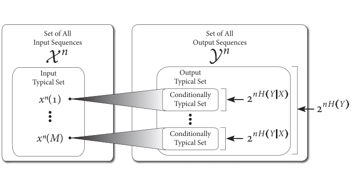
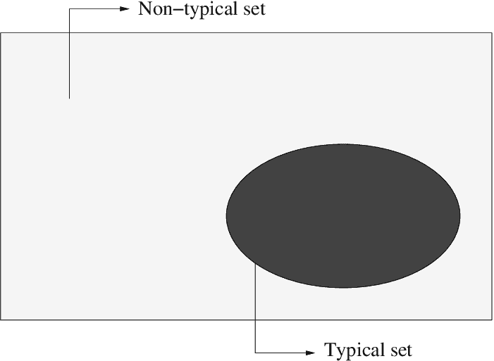
From the definition of $A_\epsilon^{(n)}$, it is clear that $A_\epsilon^{(n)}$ is a fairly small set that contains most of the probability. But from the definition, it is not clear whether it is the smallest such set. We will prove that the typical set has essentially the same number of elements as the smallest set, to first order in the exponent.

Definition For each $n=1,2, \ldots$, let $B_\delta^{(n)} \subset \mathcal{X}^n$ be the smallest set with
$$
\operatorname{Pr}\left{B_\delta^{(n)}\right} \geq 1-\delta
$$

We argue that $B_\delta^{(n)}$ must have significant intersection with $A_\epsilon^{(n)}$ and therefore must have about as many elements. In Problem 3.3.11, we outline the proof of the following theorem.

Theorem 3.3.1 Let $X_1, X_2, \ldots, X_n$ be i.i.d. $\sim p(x)$. For $\delta<\frac{1}{2}$ and any $\delta^{\prime}>0$, if $\operatorname{Pr}\left{B_\delta^{(n)}\right}>1-\delta$, then
$$
\frac{1}{n} \log \left|B_\delta^{(n)}\right|>H-\delta^{\prime} \quad \text { for } n \text { sufficiently large. }
$$
Thus, $B_\delta^{(n)}$ must have at least $2^{n H}$ elements, to first order in the exponent. But $A_\epsilon^{(n)}$ has $2^{n(H \pm \epsilon)}$ elements. Therefore, $A_\epsilon^{(n)}$ is about the same size as the smallest high-probability set.

We will now define some new notation to express equality to first order in the exponent.

数学代写|信息论作业代写information theory代考|MARKOV CHAINS

A stochastic process $\left{X_i\right}$ is an indexed sequence of random variables. In general, there can be an arbitrary dependence among the random variables. The process is characterized by the joint probability mass functions $\operatorname{Pr}\left{\left(X_1, X_2, \ldots, X_n\right)=\left(x_1, x_2, \ldots, x_n\right)\right}=p\left(x_1, x_2, \ldots, x_n\right),\left(x_1, x_2, \ldots\right.$, $\left.x_n\right) \in \mathcal{X}^n$ for $n=1,2, \ldots$.

Definition A stochastic process is said to be stationary if the joint distribution of any subset of the sequence of random variables is invariant with respect to shifts in the time index; that is,
$$
\begin{aligned}
& \operatorname{Pr}\left{X_1=x_1, X_2=x_2, \ldots, X_n=x_n\right} \
& \quad=\operatorname{Pr}\left{X_{1+l}=x_1, X_{2+l}=x_2, \ldots, X_{n+l}=x_n\right}
\end{aligned}
$$
for every $n$ and every shift $l$ and for all $x_1, x_2, \ldots, x_n \in \mathcal{X}$.

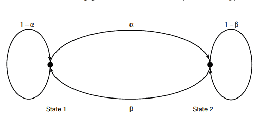
A simple example of a stochastic process with dependence is one in which each random variable depends only on the one preceding it and is conditionally independent of all the other preceding random variables. Such a process is said to be Markov.

Definition A discrete stochastic process $X_1, X_2, \ldots$ is said to be a Markov chain or a Markov process if for $n=1,2, \ldots$,
$$
\begin{aligned}
\operatorname{Pr}\left(X_{n+1}\right. & \left.=x_{n+1} \mid X_n=x_n, X_{n-1}=x_{n-1}, \ldots, X_1=x_1\right) \
& =\operatorname{Pr}\left(X_{n+1}=x_{n+1} \mid X_n=x_n\right)
\end{aligned}
$$
for all $x_1, x_2, \ldots, x_n, x_{n+1} \in \mathcal{X}$.
In this case, the joint probability mass function of the random variables can be written as
$$
p\left(x_1, x_2, \ldots, x_n\right)=p\left(x_1\right) p\left(x_2 \mid x_1\right) p\left(x_3 \mid x_2\right) \cdots p\left(x_n \mid x_{n-1}\right)
$$

信息论代写

数学代写|信息论作业代写information theory代考|HIGH-PROBABILITY SETS AND THE TYPICAL SET

从$A_\epsilon^{(n)}$的定义可以清楚地看出，$A_\epsilon^{(n)}$是一个相当小的集合，它包含了大部分的概率。但从定义来看，它是否是最小的这样的集合并不清楚。我们将证明典型集合与最小集合具有相同数量的元素，在指数上是一阶的。

定义对于每个$n=1,2, \ldots$，设$B_\delta^{(n)} \subset \mathcal{X}^n$为具有的最小集合
$$
\operatorname{Pr}\left{B_\delta^{(n)}\right} \geq 1-\delta
$$

我们认为$B_\delta^{(n)}$必须与$A_\epsilon^{(n)}$有重要的交集，因此必须有同样多的元素。在问题3.3.11中，我们概述了以下定理的证明。

定理3.3.1设$X_1, X_2, \ldots, X_n$为i.i.d $\sim p(x)$。对于$\delta<\frac{1}{2}$和任何$\delta^{\prime}>0$，如果$\operatorname{Pr}\left{B_\delta^{(n)}\right}>1-\delta$，那么
$$
\frac{1}{n} \log \left|B_\delta^{(n)}\right|>H-\delta^{\prime} \quad \text { for } n \text { sufficiently large. }
$$
因此，$B_\delta^{(n)}$必须至少有$2^{n H}$个元素，这是指数的第一阶。但是$A_\epsilon^{(n)}$有$2^{n(H \pm \epsilon)}$元素。因此，$A_\epsilon^{(n)}$与最小的高概率集大小大致相同。

现在我们将定义一些新的符号来表示指数中的一阶等式。

数学代写|信息论作业代写information theory代考|MARKOV CHAINS

随机过程$\left{X_i\right}$是随机变量的索引序列。一般来说，随机变量之间可能存在任意的依赖关系。该过程的特征是联合概率质量函数$\operatorname{Pr}\left{\left(X_1, X_2, \ldots, X_n\right)=\left(x_1, x_2, \ldots, x_n\right)\right}=p\left(x_1, x_2, \ldots, x_n\right),\left(x_1, x_2, \ldots\right.$, $n=1,2, \ldots$为$\left.x_n\right) \in \mathcal{X}^n$。

如果随机变量序列的任意子集的联合分布相对于时间指标的位移不变，则称随机过程是平稳的;也就是说，
$$
\begin{aligned}
& \operatorname{Pr}\left{X_1=x_1, X_2=x_2, \ldots, X_n=x_n\right} \
& \quad=\operatorname{Pr}\left{X_{1+l}=x_1, X_{2+l}=x_2, \ldots, X_{n+l}=x_n\right}
\end{aligned}
$$
对于每个$n$和每个班次$l$和所有$x_1, x_2, \ldots, x_n \in \mathcal{X}$。

有依赖关系的随机过程的一个简单例子是，其中每个随机变量只依赖于它前面的一个随机变量，并且有条件地独立于所有其他前面的随机变量。这样的过程被称为马尔可夫过程。

定义离散随机过程$X_1, X_2, \ldots$被称为马尔可夫链或马尔可夫过程，如果对于$n=1,2, \ldots$，
$$
\begin{aligned}
\operatorname{Pr}\left(X_{n+1}\right. & \left.=x_{n+1} \mid X_n=x_n, X_{n-1}=x_{n-1}, \ldots, X_1=x_1\right) \
& =\operatorname{Pr}\left(X_{n+1}=x_{n+1} \mid X_n=x_n\right)
\end{aligned}
$$
对于所有$x_1, x_2, \ldots, x_n, x_{n+1} \in \mathcal{X}$。
在这种情况下，随机变量的联合概率质量函数可以写成
$$
p\left(x_1, x_2, \ldots, x_n\right)=p\left(x_1\right) p\left(x_2 \mid x_1\right) p\left(x_3 \mid x_2\right) \cdots p\left(x_n \mid x_{n-1}\right)
$$

数学代写|信息论作业代写information theory代考请认准statistics-lab™

统计代写请认准statistics-lab™. statistics-lab™为您的留学生涯保驾护航。

金融工程代写

金融工程是使用数学技术来解决金融问题。金融工程使用计算机科学、统计学、经济学和应用数学领域的工具和知识来解决当前的金融问题，以及设计新的和创新的金融产品。

非参数统计代写

非参数统计指的是一种统计方法，其中不假设数据来自于由少数参数决定的规定模型；这种模型的例子包括正态分布模型和线性回归模型。

广义线性模型代考

广义线性模型（GLM）归属统计学领域，是一种应用灵活的线性回归模型。该模型允许因变量的偏差分布有除了正态分布之外的其它分布。

术语广义线性模型（GLM）通常是指给定连续和/或分类预测因素的连续响应变量的常规线性回归模型。它包括多元线性回归，以及方差分析和方差分析（仅含固定效应）。

有限元方法代写

有限元方法（FEM）是一种流行的方法，用于数值解决工程和数学建模中出现的微分方程。典型的问题领域包括结构分析、传热、流体流动、质量运输和电磁势等传统领域。

有限元是一种通用的数值方法，用于解决两个或三个空间变量的偏微分方程（即一些边界值问题）。为了解决一个问题，有限元将一个大系统细分为更小、更简单的部分，称为有限元。这是通过在空间维度上的特定空间离散化来实现的，它是通过构建对象的网格来实现的：用于求解的数值域，它有有限数量的点。边界值问题的有限元方法表述最终导致一个代数方程组。该方法在域上对未知函数进行逼近。[1] 然后将模拟这些有限元的简单方程组合成一个更大的方程系统，以模拟整个问题。然后，有限元通过变化微积分使相关的误差函数最小化来逼近一个解决方案。

tatistics-lab作为专业的留学生服务机构，多年来已为美国、英国、加拿大、澳洲等留学热门地的学生提供专业的学术服务，包括但不限于Essay代写，Assignment代写，Dissertation代写，Report代写，小组作业代写，Proposal代写，Paper代写，Presentation代写，计算机作业代写，论文修改和润色，网课代做，exam代考等等。写作范围涵盖高中，本科，研究生等海外留学全阶段，辐射金融，经济学，会计学，审计学，管理学等全球99%专业科目。写作团队既有专业英语母语作者，也有海外名校硕博留学生，每位写作老师都拥有过硬的语言能力，专业的学科背景和学术写作经验。我们承诺100%原创，100%专业，100%准时，100%满意。

随机分析代写

随机微积分是数学的一个分支，对随机过程进行操作。它允许为随机过程的积分定义一个关于随机过程的一致的积分理论。这个领域是由日本数学家伊藤清在第二次世界大战期间创建并开始的。

时间序列分析代写

随机过程，是依赖于参数的一组随机变量的全体，参数通常是时间。随机变量是随机现象的数量表现，其时间序列是一组按照时间发生先后顺序进行排列的数据点序列。通常一组时间序列的时间间隔为一恒定值（如1秒，5分钟，12小时，7天，1年），因此时间序列可以作为离散时间数据进行分析处理。研究时间序列数据的意义在于现实中，往往需要研究某个事物其随时间发展变化的规律。这就需要通过研究该事物过去发展的历史记录，以得到其自身发展的规律。

回归分析代写

多元回归分析渐进（Multiple Regression Analysis Asymptotics）属于计量经济学领域，主要是一种数学上的统计分析方法，可以分析复杂情况下各影响因素的数学关系，在自然科学、社会和经济学等多个领域内应用广泛。

MATLAB代写

MATLAB 是一种用于技术计算的高性能语言。它将计算、可视化和编程集成在一个易于使用的环境中，其中问题和解决方案以熟悉的数学符号表示。典型用途包括：数学和计算算法开发建模、仿真和原型制作数据分析、探索和可视化科学和工程图形应用程序开发，包括图形用户界面构建MATLAB 是一个交互式系统，其基本数据元素是一个不需要维度的数组。这使您可以解决许多技术计算问题，尤其是那些具有矩阵和向量公式的问题，而只需用 C 或 Fortran 等标量非交互式语言编写程序所需的时间的一小部分。MATLAB 名称代表矩阵实验室。MATLAB 最初的编写目的是提供对由 LINPACK 和 EISPACK 项目开发的矩阵软件的轻松访问，这两个项目共同代表了矩阵计算软件的最新技术。MATLAB 经过多年的发展，得到了许多用户的投入。在大学环境中，它是数学、工程和科学入门和高级课程的标准教学工具。在工业领域，MATLAB 是高效研究、开发和分析的首选工具。MATLAB 具有一系列称为工具箱的特定于应用程序的解决方案。对于大多数 MATLAB 用户来说非常重要，工具箱允许您学习和应用专业技术。工具箱是 MATLAB 函数（M 文件）的综合集合，可扩展 MATLAB 环境以解决特定类别的问题。可用工具箱的领域包括信号处理、控制系统、神经网络、模糊逻辑、小波、仿真等。

R语言代写	问卷设计与分析代写
PYTHON代写	回归分析与线性模型代写
MATLAB代写	方差分析与试验设计代写
STATA代写	机器学习/统计学习代写
SPSS代写	计量经济学代写
EVIEWS代写	时间序列分析代写
EXCEL代写	深度学习代写
SQL代写	各种数据建模与可视化代写

数学代写|信息论作业代写information theory代考|Hadamard Gate

Posted on 2023年5月16日2023年5月16日 by statistics-lab

数学代写|信息论作业代写information theory代考|Hadamard Gate

Another important unitary operator is the transformation that takes the computational basis to the $+/-$ basis. This transformation is the Hadamard transformation:
$$
|0\rangle \rightarrow|+\rangle, \quad|1\rangle \rightarrow|-\rangle
$$
Using the above relations, we can represent the Hadamard transformation as the following operator:
$$
H \equiv|+\rangle\langle 0|+|-\rangle\langle 1|
$$
It is straightforward to check that the above operator implements the transformation in (3.60).

Now consider a generalization of the above construction. Suppose that one orthonormal basis is $\left{\left|\psi_i\right\rangle\right}_{i \in{0,1}}$ and another is $\left{\left|\phi_i\right\rangle\right}_{i \in{0,1}}$ where the index $i$ merely indexes the states in each orthonormal basis. Then the unitary operator that takes states in the first basis to states in the second basis is
$$
\sum_{i=0,1}\left|\phi_i\right\rangle\left\langle\psi_i\right| .
$$
EXERCISE 3.3.7 Show that the Hadamard operator $H$ has the following matrix representation in the computational basis:
$$
H=\frac{1}{\sqrt{2}}\left[\begin{array}{cc}
1 & 1 \
1 & -1
\end{array}\right] .
$$

数学代写|信息论作业代写information theory代考|Rotation Operators

We end this section on the evolution of quantum states by discussing “rotation evolutions” and by giving a more complete picture of the Bloch sphere. The rotation operators $R_X(\phi), R_Y(\phi), R_Z(\phi)$ are functions of the respective Pauli operators $X, Y, Z$ where
$$
R_X(\phi) \equiv \exp {i X \phi / 2}, \quad R_Y(\phi) \equiv \exp {i Y \phi / 2}, \quad R_Z(\phi) \equiv \exp {i Z \phi / 2},
$$
and $\phi$ is some angle such that $0 \leq \phi<2 \pi$. How do we determine a function of an operator? The standard way is to represent the operator in its diagonal basis and apply the function to the non-zero eigenvalues of the operator. For example, the diagonal representation of the $X$ operator is
$$
X=|+\rangle\langle+|-|-\rangle\langle-|
$$
Applying the function $\exp {i X \phi / 2}$ to the non-zero eigenvalues of $X$ gives
$$
R_X(\phi)=\exp {i \phi / 2}|+\rangle\langle+|+\exp {-i \phi / 2}|-\rangle\langle-|
$$
This is a special case of the following more general convention that we follow throughout this book:

DEfinition 3.3.1 (Function of a Hermitian Operator) Suppose that a Hermitian operator $A$ has a spectral decomposition $A=\sum_{i: a_i \neq 0} a_i|i\rangle\langle i|$ for some orthonormal basis ${|i\rangle}$. Then the operator $f(A)$ for some function $f$ is defined as follows:
$$
f(A) \equiv \sum_{i: a_i \neq 0} f\left(a_i\right)|i\rangle\langle i| .
$$

信息论代写

数学代写|信息论作业代写information theory代考|Hadamard Gate

现在考虑一下上述构造的概括。假设一个标准正交基是$\left{\left|\psi_i\right\rangle\right}{i \in{0,1}}$，另一个标准正交基是$\left{\left|\phi_i\right\rangle\right}{i \in{0,1}}$，其中索引$i$仅仅索引每个标准正交基中的状态。那么将第一组基中的状态转换为第二组基中的状态的幺正算子是
$$
\sum_{i=0,1}\left|\phi_i\right\rangle\left\langle\psi_i\right| .
$$
证明Hadamard算子$H$在计算基中有如下的矩阵表示:
$$
H=\frac{1}{\sqrt{2}}\left[\begin{array}{cc}
1 & 1 \
1 & -1
\end{array}\right] .
$$

数学代写|信息论作业代写information theory代考|Rotation Operators

我们通过讨论“旋转演化”和给出布洛赫球的更完整的图像来结束量子态演化这一节。旋转算子$R_X(\phi), R_Y(\phi), R_Z(\phi)$是各自泡利算子$X, Y, Z$的函数，其中
$$
R_X(\phi) \equiv \exp {i X \phi / 2}, \quad R_Y(\phi) \equiv \exp {i Y \phi / 2}, \quad R_Z(\phi) \equiv \exp {i Z \phi / 2},
$$
$\phi$是某个角使得$0 \leq \phi<2 \pi$。我们如何确定一个算子的函数?标准的方法是在其对角基中表示算子，并将函数应用于算子的非零特征值。例如，$X$运算符的对角线表示为
$$
X=|+\rangle\langle+|-|-\rangle\langle-|
$$
将函数$\exp {i X \phi / 2}$应用于$X$的非零特征值得到
$$
R_X(\phi)=\exp {i \phi / 2}|+\rangle\langle+|+\exp {-i \phi / 2}|-\rangle\langle-|
$$
这是我们在本书中遵循的以下更一般约定的一个特例:

定义3.3.1(厄米算子的函数)假设一个厄米算子$A$对于某个标准正交基${|i\rangle}$具有谱分解$A=\sum_{i: a_i \neq 0} a_i|i\rangle\langle i|$。然后对某个函数$f$的运算符$f(A)$定义如下:
$$
f(A) \equiv \sum_{i: a_i \neq 0} f\left(a_i\right)|i\rangle\langle i| .
$$

统计代写请认准statistics-lab™. statistics-lab™为您的留学生涯保驾护航。

金融工程代写

非参数统计代写

非参数统计指的是一种统计方法，其中不假设数据来自于由少数参数决定的规定模型；这种模型的例子包括正态分布模型和线性回归模型。

广义线性模型代考

广义线性模型（GLM）归属统计学领域，是一种应用灵活的线性回归模型。该模型允许因变量的偏差分布有除了正态分布之外的其它分布。

有限元方法代写

随机分析代写

时间序列分析代写

回归分析代写

MATLAB代写

R语言代写	问卷设计与分析代写
PYTHON代写	回归分析与线性模型代写
MATLAB代写	方差分析与试验设计代写
STATA代写	机器学习/统计学习代写
SPSS代写	计量经济学代写
EVIEWS代写	时间序列分析代写
EXCEL代写	深度学习代写
SQL代写	各种数据建模与可视化代写

数学代写|信息论作业代写information theory代考|Overview

Posted on 2023年5月16日2023年5月16日 by statistics-lab

数学代写|信息论作业代写information theory代考|Overview

We first briefly overview how information is processed with quantum systems. This usually consists of three steps: state preparation, quantum operations, and measurement. State preparation is the initialization of a quantum system to some beginning state, depending on what operation we would like a quantum system to execute. There could be some classical control device that initializes the state of the quantum system. Observe that the input system for this step is a classical system, and the output system is quantum. After initializing the state of the quantum system, we perform some quantum operations that evolve its state. This stage is where we can take advantage of quantum effects for enhanced information-processing abilities. Both the input and output systems of this step are quantum. Finally, we need some way of reading out the result of the computation, and we can do so with a measurement. The input system for this step is quantum, and the output is classical. Figure 3.1 depicts all of these steps. In a quantum communication protocol, spatially separated parties may execute different parts of these steps, and we are interested in keeping track of the non-local resources needed to implement a communication protocol. Section 3.2 describes quantum states (and thus state preparation), Section 3.3 describes the noiseless evolution of quantum states, and Section 3.4 describes “read out” or measurement. For now, we assume that we can perform all of these steps perfectly and later chapters discuss how to incorporate the effects of noise.

数学代写|信息论作业代写information theory代考|Quantum Bits

The simplest quantum system is a two-state system: a physical qubit. Let $|0\rangle$ denote one possible state of the system. The left vertical bar and the right angle bracket indicate that we are using the Dirac notation to represent this state. The Dirac notation has some advantages for performing calculations in the quantum theory, and we highlight some of these advantages as we progress through our development. Let $|1\rangle$ denote another possible state of the qubit. We can encode a classical bit or cbit into a qubit with the following mapping:
$$
0 \rightarrow|0\rangle
$$
So far, nothing in our description above distinguishes a classical bit from a qubit, except for the funny vertical bar and angle bracket that we place around the bit values. However, the quantum theory predicts that the above states are not the only possible states of a qubit. Arbitrary superpositions (linear combinations) of the above two states are possible as well because the quantum theory is a linear theory. Suffice it to say that the linearity of the quantum theory results from the linearity of Schrödinger’s equation that governs the evolution of quantum systems. ${ }^1$ A general noiseless qubit can be in the following state:
$$
|\psi\rangle \equiv \alpha|0\rangle+\beta|1\rangle
$$
where the coefficients $\alpha$ and $\beta$ are arbitrary complex numbers with unit norm: $|\alpha|^2+|\beta|^2=1$. The coefficients $\alpha$ and $\beta$ are probability amplitudes-they are not probabilities themselves, but they do allow us to calculate probabilities. The unit-norm constraint leads to the Born rule (the probabilistic interpretation) of the quantum theory, and we speak more on this constraint and probability amplitudes when we introduce the measurement postulate.

信息论代写

数学代写|信息论作业代写information theory代考|Overview

我们首先简要概述量子系统是如何处理信息的。这通常包括三个步骤:状态准备、量子操作和测量。状态准备是将量子系统初始化到某个初始状态，这取决于我们希望量子系统执行什么操作。可能有一些经典的控制装置来初始化量子系统的状态。注意，这一步的输入系统是经典系统，输出系统是量子系统。在初始化量子系统的状态后，我们执行一些量子操作来演化其状态。在这个阶段，我们可以利用量子效应来增强信息处理能力。这一步的输入和输出系统都是量子的。最后，我们需要一些读出计算结果的方法，我们可以通过测量来做到这一点。这一步的输入系统是量子的，输出是经典的。图3.1描述了所有这些步骤。在量子通信协议中，空间上分离的各方可以执行这些步骤的不同部分，我们感兴趣的是跟踪实现通信协议所需的非本地资源。第3.2节描述了量子态(以及状态制备)，第3.3节描述了量子态的无噪声演化，第3.4节描述了“读出”或测量。现在，我们假设我们可以完美地执行所有这些步骤，后面的章节将讨论如何合并噪声的影响。

数学代写|信息论作业代写information theory代考|Quantum Bits

最简单的量子系统是一个双态系统:一个物理量子位。设$|0\rangle$表示系统的一种可能状态。左边的竖条和右边的尖括号表示我们用狄拉克符号来表示这个状态。狄拉克符号在量子理论的计算中有一些优势，随着我们的发展，我们将重点介绍其中的一些优势。设$|1\rangle$表示量子比特的另一种可能状态。我们可以通过以下映射将一个经典比特或cbit编码为一个量子位:
$$
0 \rightarrow|0\rangle
$$
到目前为止，在我们上面的描述中，除了我们在位值周围放置的有趣的竖条和尖括号之外，没有任何东西可以区分经典位和量子位。然而，量子理论预测上述状态并不是量子位的唯一可能状态。上述两种状态的任意叠加(线性组合)也是可能的，因为量子理论是线性理论。只要说一下，量子论的线性源于支配量子系统演化的Schrödinger方程的线性就足够了。${ }^1$一般的无噪声量子比特可以处于以下状态:
$$
|\psi\rangle \equiv \alpha|0\rangle+\beta|1\rangle
$$
其中，系数$\alpha$和$\beta$为单位范数为$|\alpha|^2+|\beta|^2=1$的任意复数。系数$\alpha$和$\beta$是概率幅值——它们本身不是概率，但它们确实允许我们计算概率。单位范数约束导致了量子理论的玻恩规则(概率解释)，当我们引入测量假设时，我们会更多地讨论这个约束和概率幅度。

统计代写请认准statistics-lab™. statistics-lab™为您的留学生涯保驾护航。

金融工程代写

非参数统计代写

非参数统计指的是一种统计方法，其中不假设数据来自于由少数参数决定的规定模型；这种模型的例子包括正态分布模型和线性回归模型。

广义线性模型代考

广义线性模型（GLM）归属统计学领域，是一种应用灵活的线性回归模型。该模型允许因变量的偏差分布有除了正态分布之外的其它分布。

有限元方法代写

随机分析代写

时间序列分析代写

回归分析代写

MATLAB代写

R语言代写	问卷设计与分析代写
PYTHON代写	回归分析与线性模型代写
MATLAB代写	方差分析与试验设计代写
STATA代写	机器学习/统计学习代写
SPSS代写	计量经济学代写
EVIEWS代写	时间序列分析代写
EXCEL代写	深度学习代写
SQL代写	各种数据建模与可视化代写

数学代写|信息论作业代写information theory代考|Data Compression

Posted on 2023年5月16日2023年5月16日 by statistics-lab

数学代写|信息论作业代写information theory代考|An Example of Data Compression

We begin with a simple example that illustrates the concept of an information source. We then develop a scheme for coding this source so that it requires fewer bits to represent its output faithfully.

Suppose that Alice is a sender and Bob is a receiver. Suppose further that a noiseless bit channel connects Alice to Bob-a noiseless bit channel is one that transmits information perfectly from sender to receiver, e.g., Bob receives “0” if Alice transmits “0” and Bob receives “1” if Alice transmits ” 1 .” Alice and Bob would like to minimize the number of times that they use this noiseless channel because it is expensive to use it.

Alice would like to use the noiseless channel to communicate information to Bob. Suppose that an information source randomly chooses from four symbols ${a, b, c, d}$ and selects them with a skewed probability distribution:
$$
\begin{aligned}
& \operatorname{Pr}{a}=1 / 2, \
& \operatorname{Pr}{b}=1 / 8, \
& \operatorname{Pr}{c}=1 / 4, \
& \operatorname{Pr}{d}=1 / 8 .
\end{aligned}
$$

So it is clear that the symbol $a$ is the most likely one, $c$ the next likely, and both $b$ and $d$ are least likely. We make the additional assumption that the information source chooses each symbol independently of all previous ones and chooses each with the same probability distribution above. After the information source makes a selection, it gives the symbol to Alice for coding.

A noiseless bit channel accepts only bits as input-it does not accept the symbols $a, b, c, d$ as input. So, Alice has to encode her information into bits. Alice could use the following coding scheme:
$$
a \rightarrow 00, \quad b \rightarrow 01, \quad c \rightarrow 10, \quad d \rightarrow 11
$$
where each binary representation of a letter is a codeword. How do we measure the performance of a particular coding scheme? The expected length of a codeword is one way to measure performance. For the above example, the expected length is equal to two bits. This measure reveals a problem with the above scheme – the scheme does not take advantage of the skewed nature of the distribution of the information source because each codeword has the same length.

One might instead consider a scheme that uses shorter codewords for symbols that are more likely and longer codewords for symbols that are less likely. ${ }^1$ Then the expected length of a codeword with such a scheme should be shorter than that in the former scheme. The following coding scheme gives an improvement in the expected length of a codeword:
$$
a \rightarrow 0, \quad b \rightarrow 110, \quad c \rightarrow 10, \quad d \rightarrow 111
$$

数学代写|信息论作业代写information theory代考|A Measure of Information

The above scheme suggests a way to measure information. Consider the probability distribution in (2.1)-(2.4). Would we be more surprised to learn that the information source produced the symbol $a$ or to learn that it produced the symbol $d$ ? The answer is $d$ because the source is less likely to produce it. Let $X$ denote a random variable with distribution given in (2.1)-(2.4). One measure of the surprise of symbol $x \in{a, b, c, d}$ is
$$
i(x) \equiv \log \left(\frac{1}{p_X(x)}\right)=-\log \left(p_X(x)\right),
$$
where the logarithm is base two-this convention implies the units of this measure are bits. This measure of surprise has the desirable property that it is higher for lower probability events and lower for higher probability events. Here, we take after Shannon, and we name $i(x)$ the information content or surprisal of the symbol $x$. Observe that the length of each codeword in the coding scheme in (2.6) is equal to the information content of its corresponding symbol.

The information content has another desirable property called additivity. Suppose that the information source produces two symbols, $x_1$ and $x_2$, with corresponding random variables $X_1$ and $X_2$. The probability for this event is $p_{X_1 X_2}\left(x_1, x_2\right)$ and the joint distribution factors as $p_{X_1}\left(x_1\right) p_{X_2}\left(x_2\right)$ if we assume the source is memoryless – that it produces each symbol independently. The information content of the two symbols $x_1$ and $x_2$ is additive because
$$
\begin{aligned}
i\left(x_1, x_2\right) & =-\log \left(p_{X_1 X_2}\left(x_1, x_2\right)\right) \
& =-\log \left(p_{X_1}\left(x_1\right) p_{X_2}\left(x_2\right)\right)
\end{aligned}
$$

$$
\begin{aligned}
& =-\log \left(p_{X_1}\left(x_1\right)\right)-\log \left(p_{X_2}\left(x_2\right)\right) \
& =i\left(x_1\right)+i\left(x_2\right)
\end{aligned}
$$
In general, additivity is a desirable property for any information measure. We will return to the issue of additivity in many different contexts in this book (especially in Chapter 13).
The expected information content of the information source is
$$
\sum_x p_X(x) i(x)=-\sum_x p_X(x) \log \left(p_X(x)\right) .
$$

信息论代写

数学代写|信息论作业代写information theory代考|An Example of Data Compression

我们从一个简单的示例开始，该示例说明了信息源的概念。然后，我们开发了一种编码该源的方案，以便它需要更少的比特来忠实地表示其输出。

假设Alice是发送者，Bob是接收者。进一步假设一条无噪声比特通道连接着Alice和Bob——无噪声比特通道是一条将信息从发送方完美地传输到接收方的通道，例如，如果Alice发送“0”，Bob接收到“0”，如果Alice发送“1”，Bob接收到“1”。Alice和Bob都希望尽量减少他们使用这个无噪声通道的次数，因为使用它的成本很高。

Alice希望使用无噪声信道向Bob传递信息。假设一个信息源从四个符号${a, b, c, d}$中随机选择，并以偏概率分布进行选择:
$$
\begin{aligned}
& \operatorname{Pr}{a}=1 / 2, \
& \operatorname{Pr}{b}=1 / 8, \
& \operatorname{Pr}{c}=1 / 4, \
& \operatorname{Pr}{d}=1 / 8 .
\end{aligned}
$$

所以很明显，符号$a$是最有可能的，$c$次之，$b$和$d$是最不可能的。我们做了一个额外的假设，即信息源独立于之前的所有符号选择每个符号，并以上述相同的概率分布选择每个符号。信息源进行选择后，将符号交给Alice编码。

一个无噪声的位通道只接受位作为输入——它不接受符号$a, b, c, d$作为输入。所以，爱丽丝必须把她的信息编码成比特。Alice可以使用以下编码方案:
$$
a \rightarrow 00, \quad b \rightarrow 01, \quad c \rightarrow 10, \quad d \rightarrow 11
$$
其中每个字母的二进制表示都是一个码字。我们如何衡量特定编码方案的性能?码字的预期长度是衡量性能的一种方法。对于上面的例子，期望的长度等于两个比特。这个度量揭示了上述方案的一个问题——该方案没有利用信息源分布的倾斜特性，因为每个码字都有相同的长度。

相反，人们可能会考虑一种方案，即对更可能出现的符号使用更短的码字，对不太可能出现的符号使用更长的码字。${ }^1$那么这种方案的码字预期长度应该比前一种方案短。以下编码方案改进了码字的预期长度:
$$
a \rightarrow 0, \quad b \rightarrow 110, \quad c \rightarrow 10, \quad d \rightarrow 111
$$

数学代写|信息论作业代写information theory代考|A Measure of Information

上述方案提出了一种测量信息的方法。考虑(2.1)-(2.4)中的概率分布。得知信息源产生了符号$a$还是得知它产生了符号$d$，我们会更惊讶吗?答案是$d$，因为来源不太可能产生它。设$X$表示一个随机变量，其分布如(2.1)-(2.4)所示。符号$x \in{a, b, c, d}$令人惊讶的一个衡量标准是
$$
i(x) \equiv \log \left(\frac{1}{p_X(x)}\right)=-\log \left(p_X(x)\right),
$$
当对数以2为底时，这种惯例意味着这种度量的单位是位。这种度量惊奇度的方法有一个可取的特性，即对于低概率事件它更高，对于高概率事件它更低。这里，我们以Shannon的名字命名为$i(x)$，表示符号$x$的信息内容或惊喜。观察式2.6中编码方案中每个码字的长度等于其对应符号的信息含量。

信息内容具有另一个理想的性质，称为可加性。假设信息源产生两个符号$x_1$和$x_2$，对应的随机变量为$X_1$和$X_2$。如果我们假设源是无记忆的，则此事件的概率为$p_{X_1 X_2}\left(x_1, x_2\right)$，联合分布因子为$p_{X_1}\left(x_1\right) p_{X_2}\left(x_2\right)$，即它独立地产生每个符号。两个符号$x_1$和$x_2$的信息内容是相加的，因为
$$
\begin{aligned}
i\left(x_1, x_2\right) & =-\log \left(p_{X_1 X_2}\left(x_1, x_2\right)\right) \
& =-\log \left(p_{X_1}\left(x_1\right) p_{X_2}\left(x_2\right)\right)
\end{aligned}
$$

$$
\begin{aligned}
& =-\log \left(p_{X_1}\left(x_1\right)\right)-\log \left(p_{X_2}\left(x_2\right)\right) \
& =i\left(x_1\right)+i\left(x_2\right)
\end{aligned}
$$
一般来说，可加性是任何信息测度的理想性质。我们将在本书的许多不同的上下文中(特别是在第13章中)回到可加性的问题。
信息源的期望信息内容为
$$
\sum_x p_X(x) i(x)=-\sum_x p_X(x) \log \left(p_X(x)\right) .
$$

统计代写请认准statistics-lab™. statistics-lab™为您的留学生涯保驾护航。

金融工程代写

非参数统计代写

非参数统计指的是一种统计方法，其中不假设数据来自于由少数参数决定的规定模型；这种模型的例子包括正态分布模型和线性回归模型。

广义线性模型代考

广义线性模型（GLM）归属统计学领域，是一种应用灵活的线性回归模型。该模型允许因变量的偏差分布有除了正态分布之外的其它分布。

有限元方法代写

随机分析代写

时间序列分析代写

回归分析代写

MATLAB代写

R语言代写	问卷设计与分析代写
PYTHON代写	回归分析与线性模型代写
MATLAB代写	方差分析与试验设计代写
STATA代写	机器学习/统计学习代写
SPSS代写	计量经济学代写
EVIEWS代写	时间序列分析代写
EXCEL代写	深度学习代写
SQL代写	各种数据建模与可视化代写

数学代写|信息论作业代写information theory代考|Representations and dilations of channels

Posted on 2023年4月23日2023年4月23日 by statistics-lab

如果你也在怎样代写信息论information theory这个学科遇到相关的难题，请随时右上角联系我们的24/7代写客服。

我们提供的信息论information theory及其相关学科的代写，服务范围广, 其中包括但不限于:

Statistical Inference 统计推断
Statistical Computing 统计计算
Advanced Probability Theory 高等概率论
Advanced Mathematical Statistics 高等数理统计学
(Generalized) Linear Models 广义线性模型
Statistical Machine Learning 统计机器学习
Longitudinal Data Analysis 纵向数据分析
Foundations of Data Science 数据科学基础

数学代写|信息论作业代写information theory代考|Stinespring representation

Recall that if $\Phi: \mathfrak{T}{+}\left(\mathbb{H}_A\right) \rightarrow \mathfrak{T}{+}\left(\mathbb{H}B\right)$ is an extended quantum channel from system $A$ to system $B$, then its dual channel $\Phi^: \mathfrak{B}\left(\mathbb{H}_B\right) \rightarrow \mathfrak{B}\left(\mathbb{H}_A\right)$ is a unital (i. e., $\Phi^\left(\mathbf{I}_B\right)=\mathbf{I}_A$ ) completely positive map (see Proposition 4.2.2). Application of the Stinespring theorem (see Theorem 4.3.1 for Stinespring representation of completely positive maps) to the dual channel $\Phi^$ yields existence of an environmental quantum system $E$ represented by the Hilbert space $\mathbb{H}_E$ and of an isometric (i. e., $\mathbf{V}^ \mathbf{V}=\mathbf{I}_A$ ) map $\mathbf{V}: \mathbb{H}_A \rightarrow \mathbb{H}_B \otimes \mathrm{H}_E$, such that $\Phi^$ can be written as $$ \Phi^(\mathbf{B})=\mathbf{V}^\left(\mathbf{B} \otimes \mathbf{I}_E\right) \mathbf{V}, \quad \forall \mathbf{B} \in \mathfrak{B}\left(\mathbb{H}_B\right), $$ where $\mathbf{I}_E$ is the identity operator on $\mathbb{H}_E$. The duality relation $\operatorname{tr}[\Phi(\rho) \mathbf{B}]=\operatorname{tr}\left[\rho \Phi^(\mathbf{B})\right]$ between $\Phi$ and $\Phi^$ yields $$ \begin{aligned} \operatorname{tr}[\Phi(\rho) \mathbf{B}] & =\operatorname{tr}\left[\rho \Phi^(\mathbf{B})\right]=\operatorname{tr}\left[\rho \mathbf{V}^\left(\mathbf{B} \otimes \mathbf{I}_E\right) \mathbf{V}\right] \ & =\operatorname{tr}\left[\mathbf{V}^\left(\mathbf{B} \otimes \mathbf{I}_E\right) \mathbf{V} \rho\right] \quad(\text { by Part } 2 \text { of Proposition 1.8.4) } \
& =\operatorname{tr}\left[\operatorname{tr}_E\left[\mathbf{V}^\left(\mathbf{B} \otimes \mathbf{I}_E\right) \mathbf{V} \rho\right]\right]=\operatorname{tr}\left[\operatorname{tr}_E\left[\mathbf{V} \rho \mathbf{V}^\left(\mathbf{B} \otimes \mathbf{I}_E\right)\right]\right] \
& =\operatorname{tr}\left[\operatorname{tr}_E\left[\mathbf{V} \rho \mathbf{V}^\right] \mathbf{B}\right], \quad \forall \rho \in \mathfrak{T}\left(\mathbb{H}_A\right) \text { and } \mathbf{B} \in \mathfrak{B}\left(\mathbb{H}_B\right) . \end{aligned} $$ Therefore, the quantum channel $\Phi: \mathfrak{T}{+}\left(\mathbb{H}A\right) \rightarrow \mathfrak{T}{+}\left(\mathbb{H}B\right)$ have the following representations in Schrodinger picture: $$ \Phi(\rho)=\operatorname{tr}_E\left[\mathbf{V} \rho \mathbf{V}^\right], \quad \forall \rho \in \mathfrak{T}{+}\left(\mathbb{H}A\right) $$ Either one of the two representations, (5.10) of $\Phi$ and (5.9) of $\Phi^$, will be called a Stinespring representation and be denoted by $\left(\mathrm{H}_E, \mathbf{V}\right)$. The Stinespring representation $\left(\mathbb{H}_E, \mathbf{V}\right)$ is called minimal if the subspace $$ \mathcal{M}=\left{\left(\mathbf{B} \otimes \mathbf{I}_E\right) \mathbf{V}|\varphi\rangle_A \mid \varphi \in \mathbb{H}_A, \mathbf{B} \in \mathfrak{B}\left(\mathbb{H}_B\right)\right} $$ is dense in $\mathbb{H}{B E}$. Stinespring’s representation is not at all unique. In fact, if $\left(\mathbb{H}E, \mathbf{V}\right)$ is a representation for the channel $\Phi^$, then it is easily seen that a further representation for $\Phi^$ is given by $\left(\mathbb{H}_E,\left(\mathbf{I}_B \otimes \mathbf{U}\right) \mathbf{V}\right)$ with any unitary $\mathbf{U} \in \mathfrak{B}\left(\mathrm{H}_B\right)$. However, it is straightforward to show that the minimal Stinespring representation is unique up to such unitary equivalence: Assume that the dual quantum channel $\Phi^$ has a minimal Stinespring representation $\left(\mathbb{H}_E, \mathbf{V}\right)$ as well as a not necessary minimal one $\left(\mathbb{H}{\tilde{E}}, \tilde{\mathbf{V}}\right)$.

数学代写|信息论作业代写information theory代考|Unitary dilation

This subsection explores different type of dilations of quantum channels as completely positive and trace-preserving maps from $\mathfrak{T}{+}\left(\mathbb{H}_A\right)$ to $\mathfrak{T}{+}\left(\mathbb{H}_B\right)$ in the Schrodinger picture and its dual channels as unital completely positive maps from $\mathfrak{B}\left(\mathrm{H}_B\right)$ to $\mathfrak{B}\left(\mathrm{H}_A\right)$ in the Heisenberg picture.

In the following, we explore unitary dilation (a special case of Stinespring dilation) and Kraus representation for quantum channels that are described in the Schrodinger picture.

The general version of unitary dilation of (extended) quantum channels from system $A$ to system $B$ holds (see Remark 5.2 below). Unfortunately, the proof is rather involved and only the case when $\mathbb{H}_A=\mathbb{H}_B=\mathbb{H}$ will be illustrated in the following result (see, e.g., Attal [3]).

Theorem 5.3.1 (Unitary dilation). Let $\mathbb{H}$ be a complex separable Hilbert space and let ( be quantum channel from $\mathbb{H}$ to $\mathbb{H}$. Then there exists a complex separable Hilbert space $\mathbb{K}$, a quantum state $\omega$ on $\mathbb{K}$ and a unitary operator $\mathbf{U}$ on $\mathrm{H} \otimes \mathbb{K}$ such that $$
\Phi(\mathbf{T})=\operatorname{tr}K\left[\mathbf{U}(\mathbf{T} \otimes \omega) \mathbf{U}^*\right], \quad \forall \mathbf{T} \in \mathfrak{T}{+}(\mathbb{H}) .
$$
Furthermore, it is always possible to choose $\mathrm{K}, \mathbf{U}$ and $\omega$ in such a way that $\omega$ is a pure state.

Proof. Let $\Phi: \mathfrak{T}{+}(\mathbb{H}) \rightarrow \mathfrak{T}{+}(\mathbb{H})$ be an extended quantum channel. Then the Kraus theorem (see Theorem 4.4.4) implies that $\Phi$ can be expressed in the form
$$
\Phi(\mathbf{T})=\sum_{i \in \mathbf{I}} \mathbf{M}i \mathbf{T} \mathbf{M}_i^, $$ in the strong convergence sense, where the $\mathbf{M}_i$ ‘s are bounded linear operators on $\mathbb{H}$ and $\sum{i \in \mathbb{I}} \mathbf{M}i^ \mathbf{M}_i=\mathbf{I}{\mathbb{H}}$. We consider the Hilbert space $\mathbb{K}$ with some orthonormal basis $\left{\psi_i\right}_{i \in \mathbb{I}}$ indexed by the same set I that contains 0 (which may be finite or countably infinite). Define the linear operator $\mathbf{V}: \mathbb{H} \otimes \mathbb{C}\left|\psi_0\right\rangle_{\mathrm{K}} \rightarrow \mathbb{H} \times \mathbb{K}$,
$$
\mathbf{V}\left(\phi \otimes \psi_0\right)=\sum_{j \in \mathbf{I}}\left(\mathbf{M}_j \phi\right) \otimes \psi_0
$$

信息论代写

数学代写|信息论作业代写information theory代考|Stinespring representation

回想一下，如果 $\Phi: \mathfrak{T}+\left(\mathbb{H}_A\right) \rightarrow \mathfrak{T}+(\mathbb{H} B)$ 是来自系统的扩展量子信道 $A$ 到系统 $B$ ，那么它的双通道 $\Phi: \mathfrak{B}\left(\mathbb{H}_B\right) \rightarrow \mathfrak{B}\left(\mathbb{H}_A\right)$ 是单位的（即， $\Phi^{\left(\mathbf{I}_B\right)}=\mathbf{I}_A$ ) 完全正映射 (见命题 4.2.2) 。Stinespring 定理 (完全正映射的 Stinespring 表示见定理 4.3.1) 在双通道中的应用〈披^产生环境量子系统的存在 $E$ 由希尔伯特空间表示 $\mathbb{H}_E$ 和一个等距的（即， $\mathbf{V}^{\mathbf{V}}=\mathbf{I}_A$ ）地图 $\mathbf{V}: \mathbb{H}_A \rightarrow \mathbb{H}_B \otimes \mathrm{H}_E$ ，这样\披^可以写成
$$
\Phi(\mathbf{B})=\mathbf{V}^{\left(\mathbf{B} \otimes \mathbf{I}_E\right)} \mathbf{V}, \quad \forall \mathbf{B} \in \mathfrak{B}\left(\mathbb{H}_B\right)
$$
在哪里 $\mathbf{I}_E$ 是身份运算符 $\mathbb{H}_E$. 二元关系 $\operatorname{tr}[\Phi(\rho) \mathbf{B}]=\operatorname{tr}[\rho \Phi(\mathbf{B})]$ 之间 $\Phi$ 和〈披人产量
因此，量子信道 $\Phi: \mathfrak{T}+(\mathbb{H} A) \rightarrow \mathfrak{T}+(\mathbb{H} B)$ 在薛定谔的图中有如下表示:
(5.10) 的两种表示之一 $\Phi$ 和 (5.9) 的披^, 将被称为 Stinespring 表示并表示为 $\left(\mathrm{H}_E, \mathbf{V}\right)$. Stinespring 代表 $\left(\mathbb{H}_E, \mathbf{V}\right)$ 称为最小的，如果子空间
密集在 $\mathbb{H} B E$. Stinespring 的代表一点也不独特。事实上，如果 $(\mathbb{H} E, \mathbf{V})$ 是通道的表示〈披人，那么很容易看出，进一步表示〈披^是 (谁) 给的 $\left(\mathbb{H}_E,\left(\mathbf{I}_B \otimes \mathbf{U}\right) \mathbf{V}\right)$ 与任何单一 $\mathbf{U} \in \mathfrak{B}\left(\mathrm{H}_B\right)$. 然而，可以直接证明最小 Stinespring 表示在这种酉等价之前是唯一的：假设双量子通道〈披^具有最小的 Stinespring 表示 $\left(\mathbb{H}_E, \mathbf{V}\right)$ 以及一个不必要的最小的 $(\mathbb{H} \tilde{E}, \tilde{\mathbf{V}})$.

数学代写|信息论作业代写information theory代考|Unitary dilation

本小节探讨了不同类型的量子通道扩张，作为来自 $\mathfrak{T}+\left(\mathbb{H}A\right)$ 到 $\mathfrak{T}+\left(\mathbb{H}_B\right)$ 在薛定谔图片及其双通道中作为单位完全正映射 $\mathfrak{B}\left(\mathrm{H}_B\right)$ 到 $\mathfrak{B}\left(\mathrm{H}_A\right)$ 在海森堡的画中。在下文中，我们探讨了酉膨胀 (Stinespring 膨胀的一个特例) 和薛定谔图片中描述的量子通道的 Kraus 表示。来自系统的 (扩展) 量子通道么正扩张的一般版本 $A$ 到系统 $B$ 持有（见下文备注 5.2）。不幸的是，证明相当复杂，而且只有在 $\mathbb{H}_A=\mathbb{H}_B=\mathbb{H}$ 将在以下结果中说明（例如，参见 Attal [3])。定理 5.3 .1 (酉膨胀) 。让 $\mathbb{H}$ 是一个复杂的可分离希尔伯特空间并且让 (是来自 $\mathbb{H}$ 到 $\mathbb{H}$. 则存在复可分希尔伯特空间 $\mathbb{K}$, 一个量子态 $\omega$ 在 $\mathbb{K}$ 和单一算子 $\mathrm{U}$ 在 $\mathrm{H} \otimes \mathbb{K}$ 这样 $$ \Phi(\mathbf{T})=\operatorname{tr} K\left[\mathbf{U}(\mathbf{T} \otimes \omega) \mathbf{U}^*\right], \quad \forall \mathbf{T} \in \mathfrak{T}+(\mathbb{H}) $$ 此外，总是可以选择K, $\mathrm{K}$ 和 $\omega$ 以这样的方式 $\omega$ 是一种纯粹的状态。证明。让 $\Phi: \mathfrak{T}+(\mathbb{H}) \rightarrow \mathfrak{T}+(\mathbb{H})$ 是一个扩展的量子信道。那么克劳斯定理（见定理 4.4.4）意味着 $\Phi$ 可以用形式表达 $$ \Phi(\mathbf{T})=\sum{i \in \mathbf{I}} \mathbf{M} i \mathbf{T} \mathbf{M}i $$ 在强收敛意义上， $\mathbf{M}_i$ 是有界线性算子 $\mathbb{H}$ 和 $\sum i \in \mathbb{I} \mathbf{M} i_i^{\mathbf{M}}=\mathbf{I H}$. 我们考虑莃尔伯特空间 $\mathbb{K}$ 有一些正交线性算子 $\mathbf{V}: \mathbb{H} \otimes \mathbb{C}\left|\psi_0\right\rangle{\mathrm{K}} \rightarrow \mathbb{H} \times \mathbb{K}$,
$$
\mathbf{V}\left(\phi \otimes \psi_0\right)=\sum_{j \in \mathbf{I}}\left(\mathbf{M}_j \phi\right) \otimes \psi_0
$$

统计代写请认准statistics-lab™. statistics-lab™为您的留学生涯保驾护航。

金融工程代写

非参数统计代写

非参数统计指的是一种统计方法，其中不假设数据来自于由少数参数决定的规定模型；这种模型的例子包括正态分布模型和线性回归模型。

广义线性模型代考

广义线性模型（GLM）归属统计学领域，是一种应用灵活的线性回归模型。该模型允许因变量的偏差分布有除了正态分布之外的其它分布。

有限元方法代写

随机分析代写

时间序列分析代写

回归分析代写

MATLAB代写

R语言代写	问卷设计与分析代写
PYTHON代写	回归分析与线性模型代写
MATLAB代写	方差分析与试验设计代写
STATA代写	机器学习/统计学习代写
SPSS代写	计量经济学代写
EVIEWS代写	时间序列分析代写
EXCEL代写	深度学习代写
SQL代写	各种数据建模与可视化代写

数学代写|信息论作业代写information theory代考|Quantum channels in the Schrodinger picture

Posted on 2023年4月23日2023年4月23日 by statistics-lab

如果你也在怎样代写信息论information theory这个学科遇到相关的难题，请随时右上角联系我们的24/7代写客服。

我们提供的信息论information theory及其相关学科的代写，服务范围广, 其中包括但不限于:

Statistical Inference 统计推断
Statistical Computing 统计计算
Advanced Probability Theory 高等概率论
Advanced Mathematical Statistics 高等数理统计学
(Generalized) Linear Models 广义线性模型
Statistical Machine Learning 统计机器学习
Longitudinal Data Analysis 纵向数据分析
Foundations of Data Science 数据科学基础

数学代写|信息论作业代写information theory代考|Quantum channels in the Schrodinger picture

Let $\mathcal{S}\left(\mathbb{H}_A\right)$ and $\mathcal{S}\left(\mathbb{H}_B\right)$ be the collections of quantum states on $\mathbb{H}_A$ and $\mathbb{H}_B$, respectively. The definition and basic properties of quantum channels in Schrodinger picture are given below.
Definition 5.2.1. A linear completely positive trace-preserving map $\Phi: \mathcal{S}\left(\mathbb{H}_A\right) \rightarrow \mathcal{S}\left(\mathbb{H}_B\right), \rho_B=\Phi\left(\rho_A\right)$, is called a quantum channel from system $A$ to system $B$. In this case, $\rho_A \in \mathcal{S}\left(\mathbb{H}_A\right)$ will be called an input state and $\rho_B \in \mathcal{S}\left(\mathbb{H}_B\right)$ will be called the output state of the channel.

The collection of quantum channels from system $A$ to system $B$ will be denoted by $\mathfrak{Q C}(A, B)$. When $\mathbb{H}_A=\mathbb{H}_B$, we will simply write $\mathfrak{Q C}(A, B)$ as $\mathfrak{Q C}(A)$.

In functional analysis, a partial isometry (see also Theorem 1.8.11 for a description) is a linear map $\Upsilon$ between Hilbert spaces $\mathbb{H}$ and $\mathbb{K}$ such that $\Upsilon$ is an isometry between $(\operatorname{ker}(\Upsilon))^{\perp} \subset \mathbb{H}$ and range $(\Upsilon) \subset \mathbb{K}$, where $(\operatorname{ker}(\Upsilon))^{\perp}$ (the orthogonal complement of its kernel) is called the initial subspace and range( $Y$ (the range of $Y$ ) is called the final subspace of the map. The concept of partial isometry can be defined in other equivalent ways. If $\mathbf{U}$ is an isometric map defined on a closed subset $\mathbb{H}_0$ of a Hilbert space $\mathbb{H}$, then we can define an extension $\mathbf{W}$ of $\mathbf{U}$ to all of $\mathbb{H}$ by the condition that $\mathbf{W}$ be zero on $\mathbb{H}_0^{\perp}$ (the orthogonal complement of $\mathbb{H}_0$ ). Thus, a partial isometry is also sometimes defined as a closed partially defined isometric map.

Definition 5.2.2 (Isometrical equivalence). Let $A, B$ and $B^{\prime}$ be quantum systems represented by the separable complex Hilbert spaces $\mathbb{H}A, \mathbb{H}_B$ and $\mathbb{H}{B^{\prime}}$, respectively. The (extended) quantum channels $\Phi: \mathfrak{T}{+}\left(\mathbb{H}_A\right) \rightarrow \mathfrak{T}{+}\left(\mathbb{H}B\right)$ and $\Phi^{\prime}: \mathfrak{T}{+}\left(\mathbb{H}A\right) \rightarrow \mathfrak{T}{+}\left(\mathbb{H}{B^{\prime}}\right)$ are said to be isometrically equivalent if there exists a partial isometry $\mathbf{W}: \mathbb{H}_B \rightarrow \mathbb{H}{B^{\prime}}$ such that
$$
\Phi^{\prime}(\rho)=\mathbf{W} \Phi(\rho) \mathbf{W}^, \quad \Phi(\rho)=\mathbf{W}^ \Phi^{\prime}(\rho) \mathbf{W}, \quad \forall \rho \in \mathfrak{T}\left(\mathbb{H}A\right) $$ The notion of isometrical equivalence is very close to the notion of unitary equivalence. Indeed, the isometrical equivalence of the channels $\Phi$ and $\Phi^{\prime}$ means unitary equivalence of these channels with the output spaces $\mathbb{H}_B$ and $\mathbb{H}{B^{\prime}}$ replaced by their subspaces $\mathbb{H}B^{\Phi}=\mathrm{V}{\rho \in \mathcal{S}\left(\mathbb{H}A\right)} \operatorname{supp}(\Phi(\rho))$ and $\mathbb{H}{B^{\prime}}^{\Phi^{\prime}}=\mathrm{V}_{\rho \in \mathcal{S}\left(\mathbb{H}_A\right)} \operatorname{supp}\left(\Phi^{\prime}(\rho)\right)$. We use the notion of isometrical equivalence, since dealing with a given representation of a quantum channel $\Phi$ it not easy in general to determine the corresponding subspace $\mathbb{H}_B^{\Phi}$. Some examples of quantum channels are given below.

数学代写|信息论作业代写information theory代考|Quantum channels in the Heisenberg picture

Without loss generality, we can and often consider the extended version of channel $\Phi: \mathfrak{T}{+}\left(\mathbb{H}_A\right) \rightarrow \mathfrak{T}{+}\left(\mathbb{H}_B\right)$ in place of the channel $\Phi: \mathcal{S}\left(\mathbb{H}_A\right) \rightarrow \mathcal{S}\left(\mathbb{H}_B\right)$ itself. In this case, $\Phi^*$, the adjoint of the (extended) quantum channel $\Phi$ is a map from $\mathfrak{B}\left(\mathbb{H}_B\right)$ to $\mathfrak{B}\left(\mathrm{H}_A\right)$. This is because $\mathfrak{T}\left(\mathbb{H}_A\right)$ and $\mathfrak{T}\left(\mathbb{H}_B\right)$ are preduals of $\mathfrak{B}\left(\mathbb{H}_A\right)$ and $\mathfrak{B}\left(\mathbb{H}_B\right)$, respectively.

Definition 5.2.3. Let $\Phi: \mathfrak{T}{+}\left(\mathbb{H}_A\right) \rightarrow \mathfrak{T}{+}\left(\mathrm{H}_B\right)$ be an (extended) quantum channel from $A$ to $B$. The adjoint operator of $\Phi, \Phi^*: \mathfrak{B}\left(\mathrm{H}_B\right) \rightarrow \mathfrak{B}\left(\mathrm{H}_A\right)$ is called the dual channel of $\mathrm{D}$.

The class of dual channels is denoted by $\mathfrak{E Q C}^(B, A)$, and similarly $\mathfrak{E Q} \mathscr{C}^(B, A)$ as $\mathfrak{E Q C} \mathcal{C}^*(A)$ if $A=B$

The (extended) quantum channels $\Phi: \mathfrak{T}{+}\left(\mathbb{H}_A\right) \rightarrow \mathfrak{T}{+}\left(\mathbb{H}B\right)$ implicitly assume the Schrodinger picture in which the states of the system are evolved while the observables of the system are kept fixed. On the other hand, the dual channel $\Phi^: \mathfrak{B}\left(\mathbb{H}_B\right) \rightarrow$ $\mathfrak{B}\left(\mathrm{H}_A\right)$ is in the Heisenberg picture and it implies that the states of the system are fixed and the observables evolve in time. The (extended) quantum channel $\Phi$ and its associated dual channel $\Phi^$, however, satisfy the following duality relation:
$$
\operatorname{tr}\left[\Phi\left(\rho_A\right) \mathbf{0}_B\right]=\operatorname{tr}\left[\rho_A \Phi^\left(\mathbf{0}_B\right)\right], \quad \forall \rho_A \in \mathfrak{T}\left(\mathbb{H}_A\right) \text { and } \forall \mathbf{0}_B \in \mathfrak{B}\left(\mathbb{H}_B\right) $$ Notice also that in the duality relation the concatenation of channels goes in reversed order in the Schrodinger picture. That is, given (extended) channels $\Phi: \mathfrak{T}{+}\left(\mathrm{H}A\right) \rightarrow$ $\mathfrak{T}{+}\left(\mathrm{H}B\right)$ and $\Psi: \mathfrak{T}{+}\left(\mathbb{H}B\right) \rightarrow \mathfrak{T}{+}\left(\mathbb{H}C\right)$, we have $$ (\Psi \circ \Phi)^=\Phi^* \circ \Psi^*
$$
A physical interpretation of the dual quantum channel $\Phi^: \mathfrak{B}\left(\mathbb{H}_B\right) \rightarrow \mathfrak{B}\left(\mathbb{H}_A\right)$ is the following: when the system is initially in the state $\rho \in \mathfrak{T}{+}\left(\mathbb{H}_A\right)$, the expectation value of the measurement of the observable $\mathbf{B} \in \mathfrak{B}\left(\mathbb{H}_B\right)$ at the output side of the channel is given in terms of $\Phi$ by $\operatorname{tr}\left[\rho \Phi^(\mathbf{B})\right]$.

The following result characterizes the dual channel $\Phi^*$ of $\Phi$, which can be viewed as the quantum channel $\Phi$ in the Heisenberg picture.

信息论代写

数学代写|信息论作业代写information theory代考|Quantum channels in the Schrodinger picture

让 $\mathcal{S}\left(\mathbb{H}A\right)$ 和 $\mathcal{S}\left(\mathbb{H}_B\right)$ 是量子态的集合 $\mathbb{H}_A$ 和 $\mathbb{H}_B$ ，分别。下面给出辠定谔图中量子通道的定义和基本性质。定义 5.2.1。一种线性完全正的保迹图 $\Phi: \mathcal{S}\left(\mathbb{H}_A\right) \rightarrow \mathcal{S}\left(\mathbb{H}_B\right), \rho_B=\Phi\left(\rho_A\right)$, 被称为系统的量子信道 $A$ 到系统 $B$. 在这种情况下， $\rho_A \in \mathcal{S}\left(\mathbb{H}_A\right)$ 将被称为输入状态和 $\rho_B \in \mathcal{S}\left(\mathbb{H}_B\right)$ 将被称为通道的输出状态。从系统中收集量子通道 $A$ 到系统 $B$ 将被表示为 $\mathfrak{Q} \mathfrak{C}(A, B)$. 什么时候 $\mathbb{H}_A=\mathbb{H}_B$ ，我们将简单地写 $\mathfrak{Q C}(A, B)$ 作为 $\mathfrak{Q C}(A)$ 之间的等距 $(\operatorname{ker}(\Upsilon))^{\perp} \subset \mathbb{H}$ 和范围 $(\Upsilon) \subset \mathbb{K}$ ，在哪里 $(\operatorname{ker}(\Upsilon))^{\perp}$ (其内核的正交补集) 称为初始子空间和范围 $(Y$ (的范围 $Y$ ) 称为映射的最终子空间。部分等距的概念可以用其他等效方式定义。如果 $U$ 是 $\mathbf{W}$ 为零 $H_0^{\perp}$ (的正交补 $\mathbb{H}_0$ ). 因此，部分等轴测图有时也被定义为封闭的部分定义等轴测图。定义 5.2.2 (等距等值) 。让 $A, B$ 和 $B^{\prime}$ 是由可分离复数桸尔伯特空间表示的量子系统 $\mathbb{H} A, \mathbb{H}_B$ 和 $\mathbb{H} B^{\prime}$ ，分别。(扩展的) 量子通道 $\Phi: \mathfrak{T}+\left(\mathbb{H}_A\right) \rightarrow \mathfrak{T}+(\mathbb{H} B)$ 和 $\Phi^{\prime}: \mathfrak{T}+(\mathbb{H} A) \rightarrow \mathfrak{T}+\left(\mathbb{H} B^{\prime}\right)$ 如果存在部分等距，则称为等距等价 $\mathbf{W}: \mathbb{H}_B \rightarrow \mathbb{H} B^{\prime}$ 这样等距等价的概念非常接近酉等价的概念。实际上，通道的等距等效性 $\Phi$ 和 $\Phi^{\prime}$ 表示这些通道与输出空间的单一等价 $\mathbb{H}_B$ 和 $\mathbb{H} B^{\prime}$ 替换为它们的子空间 $\mathbb{H} B^{\Phi}=\operatorname{V} \rho \in \mathcal{S}(\mathbb{H} A) \operatorname{supp}(\Phi(\rho))$ 和 $\mathbb{H} B^{\prime \Phi^{\prime}}=V{\rho \in \mathcal{S}\left(\mathbb{H}_A\right)} \operatorname{supp}\left(\Phi^{\prime}(\rho)\right)$. 我们使用等距等价的概念，因为处理量子通道的给定表示 $\Phi$ 一般不容易确定对应的子空间 $\mathbb{H}_B^{\Phi}$. 下面给出了一些量子信道的例子。

数学代写|信息论作业代写information theory代考|Quantum channels in the Heisenberg picture

不失一般性，我们可以并且经常考虑通道的扩展版本 $\Phi: \mathfrak{T}+\left(\mathbb{H}_A\right) \rightarrow \mathfrak{T}+\left(\mathbb{H}_B\right)$ 代替频道
$\Phi: \mathcal{S}\left(\mathbb{H}_A\right) \rightarrow \mathcal{S}\left(\mathbb{H}_B\right)$ 本身。在这种情况下， $\Phi^* ，\left(\right.$ (扩展) 量子通道的伴随 $\Phi$ 是一张地图 $\mathfrak{B}\left(\mathbb{H}_B\right)$ 到 $\mathfrak{B}\left(\mathrm{H}_A\right)$. 这是因为 $\mathfrak{T}\left(\mathbb{H}_A\right)$ 和 $\mathfrak{T}\left(\mathbb{H}_B\right)$ 是 $\mathfrak{B}\left(\mathbb{H}_A\right)$ 和 $\mathfrak{B}\left(\mathbb{H}_B\right)$ ，分别。
定义 5.2.3。让 $\Phi: \mathfrak{T}+\left(\mathbb{H}_A\right) \rightarrow \mathfrak{T}+\left(\mathrm{H}_B\right)$ 是一个 (扩展的) 量子通道 $A$ 到 $B$. 的伴随算子 $\Phi, \Phi^: \mathfrak{B}\left(\mathrm{H}_B\right) \rightarrow \mathfrak{B}\left(\mathrm{H}_A\right)$ 被称为双通道D. 双通道的类别表示为 $\mathfrak{E Q C}(B, A)$ ，同样地 $\mathfrak{E Q} \mathscr{C}(B, A)$ 作为 $\mathfrak{E Q C C} \mathcal{C}^(A)$ 如果 $A=B$
(扩展的) 量子通道 $\Phi: \mathfrak{T}+\left(\mathbb{H}_A\right) \rightarrow \mathfrak{T}+(\mathbb{H} B)$ 隐含地假设系统状态在演化而系统的可观测值保持固定的薛定谔图。另一方面，双通道 $\Phi: \mathfrak{B}\left(\mathbb{H}_B\right) \rightarrow \mathfrak{B}\left(\mathrm{H}_A\right)$ 是在海森堡的图片中，它意味着系统的状态是固定的，可观察到的是随时间演化的。（扩展的）量子通道 $\Phi$ 及其关联的双通道\披人，然而，满足以下对偶关系：
$$
\operatorname{tr}\left[\Phi\left(\rho_A\right) \mathbf{0}_B\right]=\operatorname{tr}\left[\rho_A \Phi^{\left(0_B\right)}\right], \quad \forall \rho_A \in \mathfrak{T}\left(\mathbb{H}_A\right) \text { and } \forall \mathbf{0}_B \in \mathfrak{B}\left(\mathbb{H}_B\right)
$$
还请注意，在对偶关系中，通道的串联在薛定谔图中按相反的顺序进行。也就是说，给定 (扩展) 频道 $\Phi: \mathfrak{T}+(\mathrm{H} A) \rightarrow \mathfrak{T}+(\mathrm{H} B)$ 和 $\Psi: \mathfrak{T}+(\mathbb{H} B) \rightarrow \mathfrak{T}+(\mathbb{H} C)$ ，我们有
$$
(\Psi \circ \Phi)^{=} \Phi^* \circ \Psi^*
$$
双量子通道的物理解释 $\Phi: \mathfrak{B}\left(\mathbb{H}_B\right) \rightarrow \mathfrak{B}\left(\mathbb{H}_A\right)$ 如下：当系统最初处于状态时 $\rho \in \mathfrak{T}+\left(\mathbb{H}_A\right)$, 可观测测量的期望值 $\mathbf{B} \in \mathfrak{B}\left(\mathbb{H}_B\right)$ 在通道的输出端是根据 $\Phi$ 经过 $\operatorname{tr}[\rho \Phi(\mathbf{B})]$.
以下结果表征了双通道 $\Phi^*$ 的 $\Phi$ ，可以看作是量子信道 $\Phi$ 在海森堡的画中。

统计代写请认准statistics-lab™. statistics-lab™为您的留学生涯保驾护航。

金融工程代写

非参数统计代写

非参数统计指的是一种统计方法，其中不假设数据来自于由少数参数决定的规定模型；这种模型的例子包括正态分布模型和线性回归模型。

广义线性模型代考

广义线性模型（GLM）归属统计学领域，是一种应用灵活的线性回归模型。该模型允许因变量的偏差分布有除了正态分布之外的其它分布。

有限元方法代写

随机分析代写

时间序列分析代写

回归分析代写

MATLAB代写

R语言代写	问卷设计与分析代写
PYTHON代写	回归分析与线性模型代写
MATLAB代写	方差分析与试验设计代写
STATA代写	机器学习/统计学习代写
SPSS代写	计量经济学代写
EVIEWS代写	时间序列分析代写
EXCEL代写	深度学习代写
SQL代写	各种数据建模与可视化代写

数学代写|信息论作业代写information theory代考|Probability measures on �

Posted on 2023年4月10日2023年4月10日 by statistics-lab

如果你也在怎样代写信息论information theory这个学科遇到相关的难题，请随时右上角联系我们的24/7代写客服。

我们提供的信息论information theory及其相关学科的代写，服务范围广, 其中包括但不限于:

Statistical Inference 统计推断
Statistical Computing 统计计算
Advanced Probability Theory 高等概率论
Advanced Mathematical Statistics 高等数理统计学
(Generalized) Linear Models 广义线性模型
Statistical Machine Learning 统计机器学习
Longitudinal Data Analysis 纵向数据分析
Foundations of Data Science 数据科学基础

数学代写|信息论作业代写information theory代考|Support of Borel measures

Consider the Borel measurable space $(\mathrm{X}, \mathcal{B}(\mathrm{X}))$, where $\mathrm{X}$ is a locally compact Hausdorff space (for the purpose of this book, we can simply assume that $\mathrm{X}$ is either a separable Banach or Hilbert space or a closed subset of a Banach or Hilbert space) and $\mathcal{B}(\mathrm{X})$ is the Borel $\sigma$-algebra of open subsets of $\mathrm{X}$.

We also recall some basic definitions in measure theory (see, e. g., Halmos [58] and Rudin [133]) as follows.

If $\mu: \mathcal{B}(\mathrm{X}) \rightarrow[0,+\infty]$ is a function such that (i) $\mu(B) \geq 0$ for all $B \in \mathcal{B}(\mathrm{X})$; (ii) $\mu(\emptyset)=0$ and (iii) $\mu\left(\bigcup_{i=1}^{+\infty} A_i\right)=\sum_{i=1}^{+\infty} \mu\left(A_i\right)$ for any sequence $\left(A_i\right)_{i=1}^{+\infty}$ of pairwise disjoint Borel sets (i. e., $A_i \cap A_j=\emptyset$ if $i \neq j$ ), then $\mu$ is called a Borel measure on $(\mathrm{X}, \mathcal{B}(\mathrm{X}))$. In this case, the triplet $(X, \mathcal{B}(X), \mu)$ will be referred to as a Borel measure space.
A Borel measure $\mu$ on $(X, \mathcal{B}(X))$ is said to be inner regular if
$$
\mu(B)=\sup {\mu(F) \mid \text { compact } F \subseteq B}, \quad \forall B \in \mathcal{B}(\mathrm{X})
$$
is said to be outer regular if
$$
\mu(B)=\inf {\mu(G) \mid \text { open } G \supseteq B}, \quad \forall B \in \mathcal{B}(\mathrm{X})
$$

The Borel measure $\mu$ is regular if it is both inner regular and outer regular. The Borel measure $\mu$ is said to be a Radon measure if it is both inner regular and locally finite (i. e., $\mu(F)<+\infty$ for all compact Borel set $F$ ). If the Borel measure $\mu$ is such that $\mu(\mathrm{X})=1$, then $\mu$ is called a Borel probability measure and the triplet $(\mathrm{X}, \mathcal{B}(\mathrm{X}), \mu)$ is called a Borel probability space. The collection of all Borel probability measures on $X$ will be denoted by $\mathcal{P}(\mathrm{X})$.

Without further mention, all Borel measures discussed in this book are assumed to be regular Borel measures.

数学代写|信息论作业代写information theory代考|Continuous ensembles

A Borel probability measure $\mu \in \mathcal{P}(\mathcal{S}(\mathbb{H})$ ), which is not a discrete ensemble (atomic measure), will be referred to as a continuous ensemble. The subset of $\mathcal{P}(\mathcal{S}(\mathbb{H}))$ that consists of continuous ensembles will be denoted by $\mathcal{P}^{\text {con }}(\mathcal{S}(\mathbb{H}))$. Therefore, the space $\mathcal{P}(\mathcal{S}(\mathbb{H}))$ can be decomposed as
$$
\mathcal{P}(\mathcal{S}(\mathbb{H}))=\mathcal{P}^{\mathrm{dis}}(\mathcal{S}(\mathbb{H})) \cup \mathcal{P}^{\mathrm{con}}(\mathcal{S}(\mathbb{H}))
$$
The concept of support of a Borel measure (see Definition 3.1.1) and that of spectrum (see Definition 1.4.2) of a self-adjoint linear operator on a Hilbert space are closely related (see Proposition 1.4.3).

Concepts of discrete ensemble and continuous ensembles in quantum states was first introduced in Oreshkov and Calsamiglia [120] and applied to the context of infinite-dimensional quantum information by Holevo and Shirokov [81].

Example 3.1. To explore the relation between the support of a probability measure and the spectrum of a self-adjoint linear operator on a Hilbert space, let $\mu$ be a regular Borel measure on the Borel measurable space $(\mathbb{R}, \mathcal{B}(\mathbb{R}))$. Consider the multiplication operator $(\mathbf{A} f)(x)=x f(x)$ on its natural domain $$
\operatorname{dom}(\mathbf{A})=\left{f \in L^2(\mathbb{R}, \mathcal{B}(\mathbb{R}), \mu) \mid x f(x) \in L^2(\mathbb{R}, \mathcal{B}(\mathbb{R}), \mu)\right}
$$
The multiplication operator A defined is a self-adjoint operator on the complex Hilbert space $L^2(\mathbb{R}, \mathcal{B}(\mathbb{R}), \mu)$ equipped with the inner product $\langle\cdot, \cdot\rangle_{L^2}$ (see Example 1.3 ). Indeed,
$$
\begin{aligned}
\langle f, \mathbf{A} g\rangle_{L^2} & =\int_{\mathbb{R}} \overline{f(x)} x g(x) \mu(d x) \
& =\int_{\mathbb{R}} x \overline{f(x)} g(x) \mu(d x) \
& =\langle\mathbf{A} f, g\rangle_{L^2}, \quad \forall f, g \in L^2(\mathbb{R}, \mathcal{B}(\mathbb{R}), \mu) .
\end{aligned}
$$
Thus, $\mathbf{A}$ is a self-adjoint linear operator on $L^2(\mathbb{R}, \mathcal{B}(\mathbb{R}), \mu)$ and its spectrum coincides with the essential range of the identity function, which is precisely the support of $\mu$.

信息论代写

数学代写|信息论作业代写information theory代考|Support of Borel measures

考虑 Borel 可测空间 $(\mathrm{X}, \mathcal{B}(\mathrm{X})$ ，在哪里X 是一个局部紧致的 Hausdorff 空间（就本书而言，我们可以简单地假设 $\mathrm{X}$ 是可分离的 Banach 或 Hilbert 空间或 Banach 或 Hilbert 空间的闭子集) 和 $\mathcal{B}(\mathrm{X})$ 是宝来 $\sigma$ 的开子集的代数X.
我们还回顾了测度论中的一些基本定义 (例如，参见 Halmos [58] 和 Rudin [133]) 如下。
如果 $\mu: \mathcal{B}(\mathrm{X}) \rightarrow[0,+\infty]$ 是一个函数使得 (i) $\mu(B) \geq 0$ 对全部 $B \in \mathcal{B}(\mathrm{X})$; (二) $\mu(\emptyset)=0($ (三)
$\mu\left(\bigcup_{i=1}^{+\infty} A_i\right)=\sum_{i=1}^{+\infty} \mu\left(A_i\right)$ 对于任何序列 $\left(A_i\right)_{i=1}^{+\infty}$ 成对不相交的 Borel 集（即， $A_i \cap A_j=\emptyset$ 如果
$i \neq j)$ ，然后 $\mu$ 称为 Borel 测度 $(\mathrm{X}, \mathcal{B}(\mathrm{X}))$. 在这种情况下，三胞胎 $(X, \mathcal{B}(X), \mu)$ 将被称为 Borel 测度
空间。
Borel 措施 $\mu$ 在 $(X, \mathcal{B}(X))$ 如果
$$
\mu(B)=\sup \mu(F) \mid \text { compact } F \subseteq B, \quad \forall B \in \mathcal{B}(\mathrm{X})
$$
如果
$$
\mu(B)=\inf \mu(G) \mid \operatorname{open} G \supseteq B, \quad \forall B \in \mathcal{B}(\mathrm{X})
$$
Borel 测量 $\mu$ 如果它既是内部规则又是外部规则，则它是规则的。Borel 测量 $\mu$ 如果它既是内规则的又是局部有限的（即， $\mu(F)<+\infty$ 适用于所有紧凑型 Borel 套装 $F$ ). 如果 Borel 测量 $\mu$ 是这样的 $\mu(\mathrm{X})=1$ ，然后 $\mu$ 被称为 Borel 概率测度和三元组 $(\mathrm{X}, \mathcal{B}(\mathrm{X}), \mu)$ 称为 Borel 概率空间。所有 Borel 概率测度的集合 $X$ 将被表示为 $\mathcal{P}(\mathrm{X})$.
无需进一步提及，本书中讨论的所有 Borel 测度均假定为常规 Borel 测度。

数学代写|信息论作业代写information theory代考|Continuous ensembles

Borel 概率测度 $\mu \in \mathcal{P}(\mathcal{S}(\mathbb{H})$ )，它不是离散系综（原子测度），将被称为连续系综。的子集 $\mathcal{P}(\mathcal{S}(\mathbb{H})$ )由连续系综组成的将表示为 $\mathcal{P}^{\text {con }}(\mathcal{S}(\mathbb{H}))$. 因此，空间 $\mathcal{P}(\mathcal{S}(\mathbb{H}))$ 可以分解为
$$
\mathcal{P}(\mathcal{S}(\mathbb{H}))=\mathcal{P}^{\text {dis }}(\mathcal{S}(\mathbb{H})) \cup \mathcal{P}^{\text {con }}(\mathcal{S}(\mathbb{H}))
$$
Borel 测度的支持概念 (见定义 3.1.1) 和希尔伯特空间上自伴线性算子的谱支持概念 (见定义 1.4.2) 密切相关（见命题 1.4.3) 。
量子态中离散系综和连续系综的概念首先由 Oreshkov 和 Calsamiglia [120] 引入，并由 Holevo 和 Shirokov [81] 应用于无限维量子信息的背景。
示例 3.1。为了探索概率测度的支持与希尔伯特空间上自伴线性算子的谱之间的关系，让 $\mu$ 是 Borel 可测空间上的常规 Borel 测度 $(\mathbb{R}, \mathcal{B}(\mathbb{R}))$. 考虑乘法运算符 $(\mathbf{A} f)(x)=x f(x)$ 在其自然领域
定义的乘法运算符 $\mathrm{A}$ 是复 Hilbert 空间上的自伴随运算符 $L^2(\mathbb{R}, \mathcal{B}(\mathbb{R}), \mu)$ 配备内积 $\langle\cdot, \cdot\rangle_{L^2}$ (参见示例 1.3)。的确，
$$
\langle f, \mathbf{A} g\rangle_{L^2}=\int_{\mathbb{R}} \overline{f(x)} x g(x) \mu(d x) \quad=\int_{\mathbb{R}} x \overline{f(x)} g(x) \mu(d x)=\langle\mathbf{A} f, g\rangle_{L^2}, \quad \forall f, g \in L^2(\mathbb{R}, \mathcal{B}
$$
因此， $\mathbf{A}$ 是一个自伴随线性算子 $L^2(\mathbb{R}, \mathcal{B}(\mathbb{R}), \mu)$ 其谱与恒等函数的本质范围重合，恰恰是对的支持 $\mu$.

统计代写请认准statistics-lab™. statistics-lab™为您的留学生涯保驾护航。

金融工程代写

非参数统计代写

非参数统计指的是一种统计方法，其中不假设数据来自于由少数参数决定的规定模型；这种模型的例子包括正态分布模型和线性回归模型。

广义线性模型代考

广义线性模型（GLM）归属统计学领域，是一种应用灵活的线性回归模型。该模型允许因变量的偏差分布有除了正态分布之外的其它分布。

有限元方法代写

随机分析代写

时间序列分析代写

回归分析代写

MATLAB代写

R语言代写	问卷设计与分析代写
PYTHON代写	回归分析与线性模型代写
MATLAB代写	方差分析与试验设计代写
STATA代写	机器学习/统计学习代写
SPSS代写	计量经济学代写
EVIEWS代写	时间序列分析代写
EXCEL代写	深度学习代写
SQL代写	各种数据建模与可视化代写

数学代写|信息论作业代写information theory代考|Direct sum of Hilbert spaces and operators

Posted on 2023年4月10日2023年4月10日 by statistics-lab

如果你也在怎样代写信息论information theory这个学科遇到相关的难题，请随时右上角联系我们的24/7代写客服。

我们提供的信息论information theory及其相关学科的代写，服务范围广, 其中包括但不限于:

Statistical Inference 统计推断
Statistical Computing 统计计算
Advanced Probability Theory 高等概率论
Advanced Mathematical Statistics 高等数理统计学
(Generalized) Linear Models 广义线性模型
Statistical Machine Learning 统计机器学习
Longitudinal Data Analysis 纵向数据分析
Foundations of Data Science 数据科学基础

数学代写|信息论作业代写information theory代考|Direct sum of Hilbert spaces and operators

In this section, we briefly review direct sum of Hilbert spaces and operators, which will be involved in proofs of many results in this and the next chapter.

Consider a family of complex Hilbert spaces $\left{\mathbb{H}i\right}{i \in I}$, where $\mathbb{I}$ is a finite or countably infinite index set. We define the direct sum of this family of Hilbert spaces as
$$
\bigoplus_{i \in \mathbb{I}} \mathbb{H}i=\left{\left(\psi_i\right){i \in \mathbf{I}} \in \prod_{i \in \mathbb{I}} \mathbb{H}i \mid \psi_i \in \mathbb{H}_i, i \in \mathbb{I} \text {, and } \sum{i \in \mathbb{I}}\left|\psi_i\right|_{\mathrm{H}i}^2<+\infty\right} \text {, } $$ where $\prod{i \in \mathbb{I}}$ denotes the Cartesian product and $\sum_{i \in \mathbb{I}}$ denotes the generalized sum. The direct sum $\bigoplus_{i \in \mathrm{I}} \mathbb{H}{i \in \mathrm{I}}$ is a complex Hilbert space equipped with the inner produce $\langle\cdot\rangle{\oplus} \oplus_{\mathrm{icI}} \mathrm{H}i$ defined by $$ \left\langle\left(\phi_i\right){i \in \mathbb{I}},\left(\psi_i\right){i \in \mathbb{I}}\right\rangle{\oplus_{i \in \mathbb{I}} \mathbb{H}i}=\sum{i \in \mathbb{I}}\left\langle\phi_i, \psi_i\right\rangle_{\mathrm{H}i}, \quad \forall\left(\phi_i\right){i \in \mathbb{I}},\left(\psi_i\right){i \in \mathbb{I}} \in \bigoplus{i \in \mathbb{I}} \mathbb{H}i $$ If $\mathbb{H}_i=\mathbb{H}$ for all $i \in \mathbb{I}$, one can easily prove that for each $k \in \mathbb{N}$, the $k$-fold direct sum $$ \mathbb{H}^{\oplus k}=\underbrace{\mathbb{H} \oplus \mathbb{H} \oplus \cdots \mathbb{H}}{k \text { folds }}
$$
is isomorphic to $\mathbb{C}^k \otimes \mathbb{H}$. The isomorphism between $\mathbb{H}^{\oplus k}$ and $\mathbb{C}^k \otimes \mathbb{H}$ is relevant in the context of superpositions of quantum states and entanglement.

Let $\left(\mathrm{H}n\right){n=1}^{+\infty}$ be a sequence of complex Hilbert spaces. Let $\bigoplus_{n=1}^{+\infty} \mathbb{H}n$ be the direct sum of $\left(\mathrm{H}_n\right){n=1}^{+\infty}$ (see (2.8) and (2.9) for the definition of direct sum of Hilbert spaces and related properties).

For each $n \in \mathbb{N}$, let $\mathbf{T}n \in \mathfrak{B}\left(\mathbb{H}_n\right)$ be a bounded linear operator on $\mathbb{H}_n$. We define the direct sum $\mathbf{T}=\bigoplus{n=1}^{+\infty} \mathbf{T}n: \bigoplus{n=1}^{+\infty} \mathbb{H}n \rightarrow \bigoplus{n=1}^{+\infty} \mathbb{H}n$ by $$ \mathbf{T}(\varphi)=\left(\mathbf{T}_n\left(\varphi_n\right)\right){n=1}^{+\infty}, \quad \forall \varphi=\left(\varphi_n\right){n=1}^{+\infty} \text {, } $$ where $\varphi_n \in \mathbb{H}_n$. We have the following result regarding $\mathbf{T}: \bigoplus{n=1}^{+\infty} \mathbb{H}n \rightarrow \bigoplus{n=1}^{+\infty} \mathbb{H}_n$.

数学代写|信息论作业代写information theory代考|Composite system as tensor products

The Hilbert space $\mathbb{H}$ representing a composite quantum system that consists of $n$ subsystems can be written as tensor product of $n$ Hilbert spaces of its component systems described by $\mathbb{H}1, \ldots, \mathbb{H}_n$, i. e., $\mathbb{H}=\mathbb{H}_1 \otimes \ldots \otimes \mathbb{H}_n$. In particular, for a bipartite quantum system $\mathbb{H}$ that consists of component systems $\mathbb{H}_A$ and $\mathbb{H}_B$, we write $\mathbb{H}=\mathbb{H}_A \otimes \mathbb{H}_B$ or simply $\mathbb{H}{A B}$ where the rules/properties of tensor product of Hilbert spaces and operators reviewed in Subsection 2.7.1 are applicable.

In this subsection, we are interested in computing partial traces of a bounded linear operator defined on a composite Hilbert space over each of its component Hilbert spaces.

Recall from (1.23) that $\operatorname{tr}[\mathbf{T}]$, the trace of $\mathbf{T} \in \mathcal{T}(\mathbb{H})$, is defined as $\operatorname{tr}[\mathbf{T}]=\sum_{i=1}^{+\infty}\left\langle\phi_i\right.$, $\left.\mathbf{T} \phi_i\right\rangle_{\mathbb{H}}$, where $\left{\phi_i\right}_{i=1}^{+\infty}$ is any orthonormal basis of $\mathbb{H}$.

Assume that a quantum system $A$ interacts with another quantum system $B$. In this case, the composite Hilbert space $\mathbb{H}$ can be decomposed in the form $\mathbb{H}=\mathbb{H}A \otimes \mathbb{H}_B:=$ $\mathbb{H}{A B}$, where subsystems $A$ and $B$ are represented by the complex Hilbert spaces $\mathbb{H}A$ and $\mathbb{H}_B$, respectively. The partial trace operators $\operatorname{tr}{\mathrm{H}A}[\cdots]: \tau\left(\mathbb{H}{A B}\right) \rightarrow \widetilde{I}\left(\mathbb{H}B\right)$ and $\operatorname{tr}{\mathbb{H}B}[\cdots]: \tau\left(\mathbb{H}{A B}\right) \rightarrow \tau\left(\mathbb{H}A\right)$ can be defined abstractly as $$ \operatorname{tr}{\mathrm{H}B}\left[\mathbf{T}_A \otimes \mathbf{T}_B\right]=\mathbf{T}_A \operatorname{tr}\left[\mathbf{T}_B\right] \text { and } \quad \operatorname{tr}{\mathrm{H}A}\left[\mathbf{T}_A \otimes \mathbf{T}_B\right]=\operatorname{tr}\left[\mathbf{T}_A\right] \mathbf{T}_B $$ For notational simplicity, we often write $\operatorname{tr}{\mathbb{H}A}[\cdots]$ as $\operatorname{tr}_A[\cdot], \operatorname{tr}{\mathrm{H}B}[\cdots]$ as $\operatorname{tr}_B[\cdots]$, etc. For any trace-class operator $\mathbf{T} \in \mathcal{T}\left(\mathbb{H}{A B}\right)$, we are interested in computing its partial trace $\operatorname{tr}_A[\mathbf{T}]\left(\in \mathcal{T}\left(\mathbb{H}_B\right)\right)$ taken over the Hilbert space $\mathbb{H}_A$ and partial trace $\operatorname{tr}_B[\mathbf{T}](\epsilon$ $\tau\left(\mathbb{H}_A\right)$ ) taken over $\mathbb{H}_B$. The concept of partial trace of trace-class operators on the system that consists of any finite number of subsystems can be similarly extended.

We illustrate how to compute $\operatorname{tr}B[\mathbf{T}]$ below (note that the partial trace $\operatorname{tr}_A[\mathbf{T}]$ can be similarly computed). Let $\left(\psi_i\right){i=1}^{+\infty}$ be an orthonormal basis for $\mathbb{H}B$. We consider the following isometric isomorphism: $$ \bigoplus{i=1}^{+\infty}\left(\mathbb{H}A \otimes \mathbb{C} \psi_i\right) \mapsto \mathbb{H}{A B}:=\mathbb{H}_A \otimes \mathbb{H}_B
$$

信息论代写

数学代写|信息论作业代写information theory代考|Direct sum of Hilbert spaces and operators

本节简单回顾一下Hilbert空间的直和和算子，本章和下一章的很多结果的证明都会涉及到这些。定义这个 Hilbert 空间族的直和为
在哪里 $\prod i \in \mathbb{I}$ 表示笛卡尔积和 $\sum_{i \in \mathbb{I}}$ 表示广义和。直和 $\bigoplus_{i \in \mathrm{I}} \mathbb{H} i \in \mathrm{I}$ 是一个复杂的希尔伯特空间，配备了内积 $\langle\cdot\rangle \oplus \oplus_{\mathrm{icI}} \mathrm{H} i$ 被定义为
$\left\langle\left(\phi_i\right) i \in \mathbb{I},\left(\psi_i\right) i \in \mathbb{I}\right\rangle \oplus_{i \in \mathbb{I}} \mathbb{H} i=\sum i \in \mathbb{I}\left\langle\phi_i, \psi_i\right\rangle_{\mathrm{H} i}, \quad \forall\left(\phi_i\right) i \in \mathbb{I},\left(\psi_i\right) i \in \mathbb{I} \in \bigoplus i \in \mathbb{I} \mathbb{I} i$
如果 $\mathbb{H}i=\mathbb{H}$ 对全部 $i \in \mathbb{I}$ ，可以很容易地证明，对于每个 $k \in \mathbb{N}$ ，这 $k$-折直和 $\mathbb{H}^{\oplus k}=\underbrace{\mathbb{H} \oplus \mathbb{H}^{\oplus} \oplus \cdots \mathbb{H}} k$ folds 同构于 $\mathbb{C}^k \otimes \mathbb{H}$. 之间的同构 $\mathbb{H}^{\oplus k}$ 和 $\mathbb{C}^k \otimes \mathbb{H}$ 在量子态和纠缠的叠加背景下是相关的。让 $(\mathrm{H} n) n=1^{+\infty}$ 是复数布尔伯特空间的序列。让 $\bigoplus{n=1}^{+\infty} \mathbb{H} n$ 是的直和 $\left(\mathrm{H}_n\right) n=1^{+\infty}$ (希尔伯特空间直和的定义及相关性质见 (2.8) 和 (2.9))。
对于每个 $n \in \mathbb{N}$ ，让 $T n \in \mathfrak{B}\left(\mathbb{H}_n\right)$ 是一个有界线性算子 $\mathbb{H}_n$. 我们定义直和
$\mathbf{T}=\bigoplus n=1^{+\infty} \mathbf{T} n: \bigoplus n=1^{+\infty} \mathbb{H} n \rightarrow \bigoplus n=1^{+\infty} \mathbb{H} n$ 经过
$$
\mathbf{T}(\varphi)=\left(\mathbf{T}_n\left(\varphi_n\right)\right) n=1^{+\infty}, \quad \forall \varphi=\left(\varphi_n\right) n=1^{+\infty}
$$
在哪里 $\varphi_n \in \mathbb{H}_n$. 我们有以下关于结果 $\mathbf{T}: \bigoplus n=1^{+\infty} \mathbb{H} n \rightarrow \bigoplus n=1^{+\infty} \mathbb{H}_n$.

数学代写|信息论作业代写information theory代考|Composite system as tensor products

㹷尔伯特空间 $\mathbb{H}$ 表示由以下组成的复合量子系统 $n$ 子系统可以写成张量积 $n$ 其组成系统的希尔伯特空间描 $\mathbb{H}B$ ，我们写 $\mathbb{H}=\mathbb{H}_A \otimes \mathbb{H}_B$ 或者简单地 $\mathbb{H} A B$ 在第 2.7 .1 小节中审查的希尔伯特空间和运算符的张量积的规则/属性适用的地方。在本小节中，我们感兴趣的是计算在复合 Hilbert 空间上定义的有界线性算子在其每个分量 Hilbert 空间上的部分迹。回想一下 (1.23)tr $[\mathbf{T}]$ ，的痕迹 $\mathbf{T} \in \mathcal{T}(\mathbb{H})$ ，定义为 $\operatorname{tr}[\mathbf{T}]=\sum{i=1}^{+\infty}\left\langle\phi_i, \mathbf{T} \phi_i\right\rangle_{\mathbb{H}^{\prime}}$ ，在哪里 \left {\phi_ilright $}{i=1}^{\wedge}{+\backslash$ infty $}$ 是任何正交基 $\mathbb{H}$.
假设一个量子系统 $A$ 与另一个量子系统相互作用 $B$. 在这种情况下，复合希尔伯特空间 $\mathbb{H}$ 可以分解成形式 $\mathbb{H}=\mathbb{H} A \otimes \mathbb{H}_B:=\mathbb{H} A B$ ，其中子系统 $A$ 和 $B$ 由复杂的莃尔伯特空间表示 $\mathbb{H} A$ 和 $\mathbb{H}_B$ ，分别。偏迹算子 $\operatorname{tr} H A[\cdots]: \tau(\mathbb{H} A B) \rightarrow \tilde{I}(\mathbb{H} B)$ 和 $\operatorname{tr} \mathbb{H} B[\cdots]: \tau(\mathbb{H} A B) \rightarrow \tau(\mathbb{H} A)$ 可以抽象定义为 $\operatorname{tr} \mathrm{H} B\left[\mathbf{T}_A \otimes \mathbf{T}_B\right]=\mathbf{T}_A \operatorname{tr}\left[\mathbf{T}_B\right]$ and $\quad \operatorname{tr} \mathrm{H} A\left[\mathbf{T}_A \otimes \mathbf{T}_B\right]=\operatorname{tr}\left[\mathbf{T}_A\right] \mathbf{T}_B$
为了符号简单，我们经常写 $\operatorname{tr} \mathbb{H} A[\cdots]$ 作为 $\operatorname{tr}_A[\cdot], \operatorname{tr} \mathrm{H} B[\cdots]$ 作为 $\operatorname{tr}_B[\cdots]$ 等。对于任何跟踪类运算符 $\mathbf{T} \in \mathcal{T}(\mathbb{H} A B)$ ，我们有兴趣计算它的部分踪迹 $\operatorname{tr}_A[\mathbf{T}]\left(\in \mathcal{T}\left(\mathbb{H}_B\right)\right)$ 接管希尔伯特空间 $\mathbb{H}_A$ 和部分痕迹 $\operatorname{tr}_B[\mathbf{T}]\left(\epsilon \tau\left(\mathbb{H}_A\right)\right)$ 被占领了 $\mathbb{H}_B$. 可以类似地扩展由任意有限个子系统组成的系统上的跟踪类算子的部分跟踪概念。
我们举例说明如何计算 $\operatorname{tr} B[\mathbf{T}]$ 下面（注意部分跟踪 $\operatorname{tr}_A[\mathbf{T}]$ 可以类似地计算）。让 $\left(\psi_i\right) i=1^{+\infty}$ 是正交基础 $\mathbb{H} B$. 我们考虑以下等距同构:
$$
\bigoplus i=1^{+\infty}\left(\mathbb{H} A \otimes \mathbb{C} \psi_i\right) \mapsto \mathbb{H} A B:=\mathbb{H}_A \otimes \mathbb{H}_B
$$

统计代写请认准statistics-lab™. statistics-lab™为您的留学生涯保驾护航。

金融工程代写

非参数统计代写

非参数统计指的是一种统计方法，其中不假设数据来自于由少数参数决定的规定模型；这种模型的例子包括正态分布模型和线性回归模型。

广义线性模型代考

广义线性模型（GLM）归属统计学领域，是一种应用灵活的线性回归模型。该模型允许因变量的偏差分布有除了正态分布之外的其它分布。

有限元方法代写

随机分析代写

时间序列分析代写

回归分析代写

MATLAB代写

R语言代写	问卷设计与分析代写
PYTHON代写	回归分析与线性模型代写
MATLAB代写	方差分析与试验设计代写
STATA代写	机器学习/统计学习代写
SPSS代写	计量经济学代写
EVIEWS代写	时间序列分析代写
EXCEL代写	深度学习代写
SQL代写	各种数据建模与可视化代写

数学代写|信息论作业代写information theory代考|INFM130

Posted on 2023年3月30日2023年3月30日 by statistics-lab

如果你也在怎样代写信息论information theory这个学科遇到相关的难题，请随时右上角联系我们的24/7代写客服。

我们提供的信息论information theory及其相关学科的代写，服务范围广, 其中包括但不限于:

Statistical Inference 统计推断
Statistical Computing 统计计算
Advanced Probability Theory 高等概率论
Advanced Mathematical Statistics 高等数理统计学
(Generalized) Linear Models 广义线性模型
Statistical Machine Learning 统计机器学习
Longitudinal Data Analysis 纵向数据分析
Foundations of Data Science 数据科学基础

数学代写|信息论作业代写information theory代考|Bounded linear operators

Let $\mathrm{X}$ and $\mathrm{Y}$ be complex Banach spaces (or Hilbert spaces) equipped with the norm $|\cdot|_{\mathrm{X}}$ and $|\cdot|_{\mathrm{Y}}$, respectively.

A linear map $\mathbf{T}: \operatorname{dom}(\mathbf{T}) \subset X \rightarrow \mathbb{Y}$ is said to be a bounded linear map if $\mathbf{T}(B)$ is a bounded subset of $Y$ for every bounded $B \subset \operatorname{dom}(\mathbf{T}) \subset X$. Equivalently, $T$ is a bounded linear map if there exists a constant $K>0$ (that depends on $\mathrm{T}$ only) such that
$$
|\mathrm{T} \psi|_{\mathrm{Y}} \leq K|\psi|_{\mathrm{X}}, \quad \forall \psi \in \operatorname{dom}(\mathrm{T}) \subset \mathrm{X}
$$

In this case, it can be proved (see, e. g., Reed and Simon [128] and Rudin [134]) that $\operatorname{dom}(\mathbf{T})=\mathbf{X}$. The collection of bounded linear maps from $\mathbb{X}$ to $\mathbb{Y}$ will be denoted by $\mathfrak{B}(\mathbb{X}, \mathbf{Y})$. If $\mathbb{X}=\mathbb{Y}$, then $\mathfrak{B}(\mathbb{X}, \mathbf{Y})$ can be written as $\mathfrak{B}(\mathbb{X})$ and $\mathbf{T} \in \mathfrak{B}(\mathbb{X})$ will be called a bounded linear operator.

The following is a Banach-Schauder theorem, which is also known as an open mapping theorem. A proof can be found in standard functional analysis texts such as Rudin [133] and is omitted here.

Theorem 1.2.1 (Banach-Schauder theorem). If $\mathrm{X}$ and $\mathrm{Y}$ are complex Banach spaces or complex Hilbert spaces and $\mathbf{T}: \mathbb{X} \rightarrow \mathbb{Y}$ is a surjective (or onto) bounded linear operator, then $\mathbf{T}$ is an open map (i.e., if $U$ is an open set in $\mathbf{X}$, then $\mathbf{T}(U)$ is open in $\mathbb{Y}$ ).
We have the following corollary.
Corollary 1.2.2. If $\mathrm{X}$ and $\mathrm{Y}$ are complex Banach or Hilbert spaces and $\mathbf{T} \in \mathcal{L}(\mathbb{X}, \mathbb{Y})$ is invertible (i.e., a bijective linear map), then the inverse map, $\mathbf{T}^{-1}$, is bounded, i. e., $\mathbf{T}^{-1} \in \mathfrak{B}(\mathbf{Y}, \mathbf{X})$. (Note that $\mathbf{T}^{-1}$ is automatically linear.)
If $\mathbf{T} \in \mathfrak{B}(\mathbb{X})$, we define the operator norm $|\mathbf{T}|_{\infty}$ of $\mathbf{T}$ as
$$
|\mathbf{T}|_{\infty}=\sup {\phi \neq 0} \frac{|\mathbf{T} \phi|{\mathrm{X}}}{|\phi|_{\mathrm{X}}}=\sup {|\phi|{\mathrm{X}}=1}|\mathbf{T} \phi|_{\mathrm{X}}
$$
There are two trivial bounded linear operators $\mathbf{0}{\mathbf{X}}$ (the zero operator) and $\mathbf{I}{\mathbf{X}}$ (the identity operator) that will appear often throughout the book. The zero operator $\mathbf{0}{\mathrm{X}}$ is the operator that maps every vector $\phi \in \mathbb{X}$ to the zero vector $\mathbf{0}$ in X (i. e., $\mathbf{0}{\mathrm{X}} \phi=\mathbf{0}$ for all $\phi \in \mathbb{X})$ and the identity operator $\mathbf{I}{\mathrm{H}}$ is the operator that maps every vector $\phi \in \mathbb{X}$ to itself (i. e., $\mathbf{I}{\mathbf{X}} \phi=\phi$ for all $\phi \in \mathrm{X}$.)

数学代写|信息论作业代写information theory代考|Positive operators

A linear (but not necessary bounded) operator $\mathbf{T} \in \mathfrak{L}(\mathbb{H})$ on a complex Hilbert space $\mathbb{H}$ is said to be positive and to be denoted by $\mathbf{T} \geq \mathbf{0}$ if $\langle\mathbf{T} \varphi, \varphi\rangle_{\mathbf{H}} \geq 0$ for all $\varphi \in \operatorname{dom}(\mathbf{T})$.

Let $\mathbf{T}_1, \mathbf{T}_2 \in \mathfrak{L}(\mathbb{H})$. We say that $\mathbf{T}_1 \geq \mathbf{T}_2$ if $\mathbf{T}_1-\mathbf{T}_2:=\mathbf{T}_1+\left(-\mathbf{T}_2\right) \geq \mathbf{0}$, where $-\mathbf{T}$ is the linear operator such that $\mathbf{T}+(-\mathbf{T})=\mathbf{0}$.

The set of all positive linear operators (resp., positive bounded linear operators) on $\mathbb{H}$ will be denoted by $\mathfrak{L}{+}(\mathbb{H})$ (resp., $\mathfrak{B}{+}(\mathbb{H})$ ). Both $\mathfrak{L}{+}(\mathbb{H})$ and $\mathfrak{B}{+}(\mathbb{H})$ are positive cones in the sense that $\mathbf{T} \in \mathfrak{L}{+}(\mathbb{H})$ (resp., $\mathfrak{B}{+}(\mathbb{H})$ ) and $c>0$ imply that $c \mathbf{T} \in \mathfrak{L}{+}(\mathbb{H})$ (resp., $\left.\mathfrak{B}{+}(\mathbb{H})\right)$

A sequence of bounded linear operators $\left(\mathbf{A}n\right){n=1}^{+\infty} \subset \mathfrak{B}(\mathbb{H})$ is said to converge strongly to $\mathbf{A} \in \mathfrak{B}(\mathbb{H})$ if
$$
\lim {n \rightarrow+\infty}\left|\mathbf{A}_n \phi-\mathbf{A} \phi\right|{\mathrm{H}}=0, \quad \forall \phi \in \mathbb{H}
$$
We will use the following monotone convergence theorem of a sequence of nondecreasing positive bounded linear operators.

Theorem 1.3.1 (Monotone convergence theorem for operators). Let $\quad\left(\mathbf{A}n\right){n=1}^{+\infty}$ be $a$ bounded monotone sequence of bounded linear operators on $\mathbb{H}$. Then the sequence $\left(\mathbf{A}n\right){n=1}^{+\infty}$ is strongly convergent.
Proof. Assume, for example, that $\left(\mathbf{A}n\right){n=1}^{+\infty}$ is such that
$$
\mathbf{A}1 \leq \mathbf{A}_2 \leq \cdots \leq \mathbf{A}_n \leq \cdots \leq \mathbf{M} $$ for some $\mathbf{M} \in \mathfrak{B}(\mathbb{H})$. Since $\sup _n\left|\mathbf{A}_n\right|{\infty} \leq|\mathbf{M}|_{\infty}<+\infty$, we obtain that for any $\phi \in \mathbb{H}$ the sequence $\left\langle\mathbf{A}n \phi, \phi\right\rangle{\mathbb{H}}$ is convergent. Therefore, due to “polarization” (1.13),
$$
\begin{aligned}
\left\langle\mathbf{A}n \phi, \psi\right\rangle & =\frac{1}{4}\left{\left\langle\mathbf{A}_n(\phi+\psi), \phi+\psi\right\rangle{\mathbb{H}}-\left\langle\mathbf{A}n(\phi-\psi), \phi-\psi\right\rangle{\mathbb{H}}\right. \
& \left.+\iota\left[\left\langle\mathbf{A}n(\phi+\imath \psi), \phi+\imath \psi\right\rangle{\mathbb{H}}-\left\langle\mathbf{A}n(\phi-\imath \psi), \phi-\imath \psi\right\rangle{\mathbf{H}}\right]\right} .
\end{aligned}
$$

信息论代写

数学代写|信息论作业代写information theory代考|Bounded linear operators

让 $X$ 和 $Y$ 是配备规范的复杂 Banach 空间 (或 Hilbert 空间) $|\cdot|{ }X$ 和 $|\cdot|_Y$ ，分别。线性映射 $\mathbf{T}: \operatorname{dom}(\mathbf{T}) \subset X \rightarrow \mathbb{Y}$ 被称为有界线性映射如果 $\mathbf{T}(B)$ 是的有界子集 $Y$ 对于每一个有界 $B \subset \operatorname{dom}(\mathbf{T}) \subset X$. 等价地， $T$ 是有界线性映射，如果存在常数 $K>0$ (这取决于 $\mathrm{T}$ 仅) 这样 $$ |\mathrm{T} \psi|{\mathrm{Y}} \leq K|\psi|{\mathrm{X}}, \quad \forall \psi \in \operatorname{dom}(\mathrm{T}) \subset \mathrm{X} $$ 在这种情况下，可以证明（参见 Reed 和 Simon [128] 以及 Rudin [134]) $\operatorname{dom}(\mathbf{T})=\mathbf{X}$. 有界线性映射的集合来自 $\mathbb{X}$ 到 $\mathbb{Y}$ 将被表示为 $\mathfrak{B}(\mathbb{X}, \mathbf{Y})$. 如果 $\mathbb{X}=\mathbb{Y}$ ，然后 $\mathfrak{B}(\mathbb{X}, \mathbf{Y})$ 可以写成 $\mathfrak{B}(\mathbb{X})$ 和 $\mathbf{T} \in \mathfrak{B}(\mathbb{X})$ 将被称为有界线性算子。以下是 Banach-Schauder 定理，也称为开映射定理。可以在 Rudin [133] 等标准功能分析文本中找到证明，此处省略。定理 1.2.1 (Banach-Schauder 定理) 。如果X和 $Y$ 是复 Banach 空间或复 Hilbert 空间和 $\mathbf{T}: \mathbb{X} \rightarrow \mathbb{Y}$ 是满射 (或满射) 有界线性算子，则 $\mathbf{T}$ 是一个开放映射 (即，如果 $U$ 是一个开集 $\mathbf{X}$ ，然后 $\mathbf{T}(U)$ 打开于 $\mathbb{Y}$ ). 我们有以下推论。推论 1.2.2。如果 $X$ 和 $Y$ 是复 Banach 或 Hilbert 空间和 $\mathbf{T} \in \mathcal{L}(\mathbb{X}, \mathbb{Y})$ 是可逆的（即双射线生映射)，那么逆映射， $\mathbf{T}^{-1}$ ，是有界的，即 $\mathbf{T}^{-1} \in \mathfrak{B}(\mathbf{Y}, \mathbf{X})$. (注意 $\mathbf{T}^{-1}$ 是自动线性的。) 如果 $\mathbf{T} \in \mathfrak{B}(\mathbb{X})$ ，我们定义算子范数 $|\mathbf{T}|{\infty}$ 的 $\mathbf{T}$ 作为
$$
|\mathbf{T}|{\infty}=\sup \phi \neq 0 \frac{|\mathbf{T} \phi| \mathrm{X}}{|\phi|{\mathrm{X}}}=\sup |\phi| \mathrm{X}=1|\mathbf{T} \phi|_{\mathrm{X}}
$$
有两个平凡的有界线生算子 $\mathbf{0 X}$ (零运算符) 和IX (身份运算符) 将在整本书中经常出现。零运算符 $\mathbf{O X}$ 是映射每个向量的运算符 $\phi \in \mathbb{X}$ 到零向量 0 在 X (即 $0 \mathrm{X} \phi=\mathbf{0}$ 对全部 $\phi \in \mathbb{X}$ )和身份运营商IH是映射每个向量的运算符 $\phi \in \mathbb{X}$ 对自己 (即IXX $\phi=\phi$ 对全部 $\phi \in \mathbf{X}$.)

数学代写|信息论作业代写information theory代考|Positive operators

线性 (但不一定有界) 运算符 $\mathbf{T} \in \mathfrak{L}(\mathbb{H})$ 在复杂的 Hilbert 空间上 $\mathbb{H}$ 据说是积极的，并表示为 $\mathbf{T} \geq \mathbf{0}$ 如果 $\langle\mathbf{T} \varphi, \varphi\rangle_{\mathbf{H}} \geq 0$ 对全部 $\varphi \in \operatorname{dom}(\mathbf{T})$.
让 $\mathbf{T}1, \mathbf{T}_2 \in \mathfrak{L}(\mathbb{H})$. 我们说 $\mathbf{T}_1 \geq \mathbf{T}_2$ 如果 $\mathbf{T}_1-\mathbf{T}_2:=\mathbf{T}_1+\left(-\mathbf{T}_2\right) \geq \mathbf{0}$ ，在哪里 $-\mathbf{T}$ 是这样的线性算子 $\mathbf{T}+(-\mathbf{T})=\mathbf{0}$ 上所有正线性算子 (分别为正有界线性算子) 的集合茑将被表示为 $\mathfrak{L}+(\mathbb{H})$ (分别， $\mathfrak{B}+(\mathbb{H})$ ). 两个都 $\mathfrak{L}+(\mathbb{H})$ 和 $\mathfrak{B}+(\mathbb{H})$ 在某种意义上是正锥 $\mathbf{T} \in \mathfrak{L}+(\mathbb{H})$ (分别， $\mathfrak{B}+(\mathbb{H})$ ) 和 $c>0$ 暗示 $c \mathbf{T} \in \mathfrak{L}+(\mathbb{H})$ $($ 分别， $\mathfrak{B}+(\mathbb{H}))$ 有界线性算子序列 $(\mathbf{A} n) n=1^{+\infty} \subset \mathfrak{B}(\mathbb{H})$ 据说强烈收敛到 $\mathbf{A} \in \mathfrak{B}(\mathbb{H})$ 如果 $$ \lim n \rightarrow+\infty\left|\mathbf{A}_n \phi-\mathbf{A} \phi\right| \mathrm{H}=0, \quad \forall \phi \in \mathbb{H} $$ 我们将使用以下一系列非递减正有界线性算子的单调收敛定理。定理 1.3.1 (算子的单调收敛定理) 。让 $(\mathbf{A} n) n=1^{+\infty}$ 是 $a$ 有界线性算子的有界单调序列 $\mathbb{H}$. 然后顺序 $(\mathbf{A} n) n=1^{+\infty}$ 是强收敛的。证明。例如，假设 $(\mathbf{A} n) n=1^{+\infty}$ 是这样的 $$ \mathbf{A} 1 \leq \mathbf{A}_2 \leq \cdots \leq \mathbf{A}_n \leq \cdots \leq \mathbf{M} $$ 对于一些 $\mathbf{M} \in \mathfrak{B}(\mathbb{H})$. 自从 $\sup _n\left|\mathbf{A}_n\right| \infty \leq|\mathbf{M}|{\infty}<+\infty$ ，我们得到任何 $\phi \in \mathbb{H}$ 序列 $\langle\mathbf{A} n \phi, \phi\rangle \mathbb{H}$ 是收敛的。因此，由于”极化” (1.13)，

统计代写请认准statistics-lab™. statistics-lab™为您的留学生涯保驾护航。

金融工程代写

非参数统计代写

非参数统计指的是一种统计方法，其中不假设数据来自于由少数参数决定的规定模型；这种模型的例子包括正态分布模型和线性回归模型。

广义线性模型代考

广义线性模型（GLM）归属统计学领域，是一种应用灵活的线性回归模型。该模型允许因变量的偏差分布有除了正态分布之外的其它分布。

有限元方法代写

随机分析代写

时间序列分析代写

回归分析代写

MATLAB代写

R语言代写	问卷设计与分析代写
PYTHON代写	回归分析与线性模型代写
MATLAB代写	方差分析与试验设计代写
STATA代写	机器学习/统计学习代写
SPSS代写	计量经济学代写
EVIEWS代写	时间序列分析代写
EXCEL代写	深度学习代写
SQL代写	各种数据建模与可视化代写

数学代写|信息论作业代写information theory代考|CSYS5030

Posted on 2023年3月30日2023年3月30日 by statistics-lab

如果你也在怎样代写信息论information theory这个学科遇到相关的难题，请随时右上角联系我们的24/7代写客服。

我们提供的信息论information theory及其相关学科的代写，服务范围广, 其中包括但不限于:

Statistical Inference 统计推断
Statistical Computing 统计计算
Advanced Probability Theory 高等概率论
Advanced Mathematical Statistics 高等数理统计学
(Generalized) Linear Models 广义线性模型
Statistical Machine Learning 统计机器学习
Longitudinal Data Analysis 纵向数据分析
Foundations of Data Science 数据科学基础

数学代写|信息论作业代写information theory代考|Complex Hilbert and Banach spaces

This section serves as a review of complex Hilbert and Banach spaces. Some of the frequently used theorems and/or propositions are stated without a proof.

Complex Hilbert spaces play an important role in the description of quantum systems. As mentioned in Chang [24], every quantum system is associated with an infinite-dimensional separable or a finite-dimensional complex Hilbert space, which consists of the states of the quantum system. In physics terminology, the Hilbert space is usually referred to as the space of (pure) states. Throughout this monograph, the mathematical description of a quantum system shall be based on a certain complex (separable) Hilbert space $\mathbb{H}$ and, therefore, the quantum system will simply be denoted by $\mathbb{H}$.

The quantum system $\mathbb{H}$ is said to be a finite-dimensional system if $\mathbb{H}$ is a finitedimensional complex Hilbert space. Otherwise, the quantum system $\mathbb{H}$ is said to be an infinite-dimensional system.
We first set some basic notation below.
Let $\mathbb{R}$ and $\mathbb{C}$ denote the field of real numbers and the field of complex numbers, respectively. If $z=x+i y \in \mathbb{C}$, where $x, y \in \mathbb{R}$, let $\bar{z}=x-i y \in \mathbb{C}$ and $|z|=\sqrt{x^2+y^2} \in$ $\mathbb{R}_{+}$denote the complex conjugate and the modulus of the complex number $z \in \mathbb{C}$, respectively. In this case, $x=\mathbb{R}(z)$ is the real part of $z$ and $y=J(z)$ is the imaginary part of $z$. Throughout the end, elements in $\mathbb{R}$ or $\mathbb{C}$ shall be denoted by lowercase letters such as $a, b$ or $c$ and sometimes lower case Greek alphabets such as $\lambda$ and $\alpha$.
We also use the following conventional notation throughout the book:

$\quad \mathbb{N}$ is the set of all natural numbers, positive integers, i. e., $\mathbb{N}={1,2, \cdots, n, \cdots}$.
$\mathbb{Z}$ is the set of all integers, i. e., $\mathbb{Z}={\cdots,-2,-1,0,1,2, \cdots}$.
$\mathbb{Z}{+}$is the set of nonnegative integers, i. e., $\mathbb{Z}{+}=\mathbb{N} \cup{0}$.
$-\mathbb{R}_{+}={c \in \mathbb{R} \mid c \geq 0}$.
For – $\infty a<b<+\infty$, we use the usual convention for closed, open and halfopen intervals on the real line $\mathbb{R}$ such as $[a, b],[a, b[] a, b],]-\infty, a],]-\infty, a[$, $[b,+\infty[$ and $] b, \infty[$, etc.

Let $\mathbb{H}$ be a (generic) Hilbert space over the field of complex numbers $\mathbb{C}$ and be referred to as a complex Hilbert space throughout the end.

数学代写|信息论作业代写information theory代考|Linear operators and their adjoints

Let $\mathrm{X}$ and $\mathrm{Y}$ be two separable complex Banach spaces equipped with Banach norms $|\cdot|_{\mathrm{X}}$ and $|\cdot|_{\mathrm{Y}}$, respectively.
A map (or transformation) $\mathbf{T}: \operatorname{dom}(\mathbf{T}) \subseteq \mathbb{X} \rightarrow \mathbb{Y}$ is said to be linear if
$$
a \phi+b \psi \in \operatorname{dom}(\mathbf{T})
$$
and
$$
\mathbf{T}(a \phi+b \psi)=a \mathbf{T}(\phi)+b \mathbf{T}(\psi), \quad \forall a, b \in \mathbb{C} \text { and } \forall \phi, \psi \in \operatorname{dom}(\mathbf{T})
$$
where $\operatorname{dom}(\mathbf{T}) \subseteq \mathbf{X}$ is called the domain of $\mathbf{T}$. Note that dom $(\mathbf{T}) \neq \mathbf{X}$, in general. However, it is known that dom(T) is a dense subset of $X$.
The following are some known cases where $\operatorname{dom}(T)=X$ :
(i) $\mathbf{T}$ is a bounded linear operator (see the following subsection for the definition of a bounded linear operator);
(ii) $\mathbb{X}=\mathbb{H}$ is a Hilbert space and $\operatorname{dim}(\mathbb{H})<+\infty$, where $\operatorname{dim}(\mathbb{H})$ denotes the dimension of $\mathbb{H}$. In this case, every linear operator is a bounded linear operator (see (1.10) below for the definition of a bounded linear operator).

Assuming dom $(T)$ is dense in $\mathrm{X}$ or $\operatorname{dom}(T)=X$, the collection of such linear maps will be denoted by $\mathfrak{L}(X, \mathbb{Y})$. The linear map T will be called a linear operator if $\operatorname{dom}(\mathbf{T}) \subseteq$ $X=\mathbb{Y}$. The collection of linear operators will be denoted by $\mathcal{L}(X)$.

Throughout to the end, linear maps/operators on a complex Banach or Hilbert space will be denoted by boldfaced letters such as $\mathbf{S}, \mathbf{T}, \mathbf{a}, \mathbf{b}, \mathbf{X}, \mathbf{Y}$, etc., and a linear $\operatorname{map} T \in \mathfrak{L}(\mathbb{X}, \mathrm{Y})$ acting on a vector $\phi \in \mathbb{X}$ will be denoted by either $\mathbf{T} \phi$ or $\mathbf{T}(\phi)$.

Let $\mathbf{T}: \operatorname{dom}(\mathbf{T}) \rightarrow \operatorname{range}(\mathbf{T})$ (where $\operatorname{range}(\mathbf{T}):={\mathbf{T} \phi \in \mathbb{Y} \mid \phi \in \operatorname{dom}(\mathbf{T}) \subset \mathbf{X}}$ denotes the range of $\mathbf{T}$ ) be a bijective (one-to-one and onto) linear map. A linear map $\mathbf{S}:$ range(T) $\rightarrow \operatorname{dom}(\mathbf{S})$ is said to be the inverse of $\mathbf{T}$ if $\mathbf{S} \circ \mathbf{T}=\mathbf{I}{\mathbf{X}}$ and $\mathbf{T} \circ \mathbf{S}=\mathbf{I}{\mathbb{Y}}$, where $\mathbf{I}{\mathrm{X}}$ and $\mathbb{I}{\mathrm{Y}}$ are the identity operator on $\mathrm{X}$ and $\mathbb{Y}$, respectively. That is, $\mathbf{I}{\mathbf{X}}(x)=x$ for all $x \in \mathbb{X}$ and $\mathbf{I}{\mathrm{Y}}(y)=y$ for all $y \in \mathbb{Y}$. In this case, we write $\mathbf{S}=\mathbf{T}^{-1}$.

For a linear map $\mathbf{T}: \operatorname{dom}(\mathbf{T}) \subset \mathbb{H} \rightarrow \mathbb{K}$, where $\mathbb{H}$ and $\mathbb{K}$ are complex Hilbert spaces, $\operatorname{ker}(\mathbf{T})$ (the kernel of $\mathbf{T}$ ), range(T) (the range of $\mathbf{T}$ ) and $\operatorname{supp}(\mathbf{T}$ ) (the support of T) are defined as:
$$
\begin{aligned}
\operatorname{ker}(\mathbf{T}) & ={\phi \in \operatorname{dom}(\mathbf{T}) \subset \mathbb{H} \mid \mathbf{T} \phi=0} \
\operatorname{range}(\mathbf{T}) & ={\psi \in \mathbb{K} \mid \psi=\mathbf{T} \phi \text { for some } \phi \in \operatorname{dom}(\mathbf{T}) \subset \mathbb{H}} \
\operatorname{supp}(\mathbf{T}) & =(\operatorname{ker}(\mathbf{T}))^{\perp}:=\left{\psi \in \mathbb{H} \mid\langle\psi, \phi\rangle_{\mathbf{H}}=0, \forall \phi \in \operatorname{ker}(\mathbf{T})\right}
\end{aligned}
$$
A linear map $\mathbf{T}: \operatorname{dom}(\mathbf{T}) \rightarrow \mathbb{K}$ is said to be closed if its graph,
$$
\operatorname{graph}(\mathbf{T}):={(\phi, \mathbf{T}(\phi)) \in \mathbb{H} \times \mathbb{K} \mid \phi \in \operatorname{dom}(\mathbf{T})}
$$
is a closed subset of $\mathbb{H} \times \mathbb{K}$.

信息论代写

数学代写|信息论作业代写information theory代考|Complex Hilbert and Banach spaces

本节回顾复数 Hilbert 和 Banach 空间。一些常用的定理和/或命题在没有证明的情况下陈述。
复 Hilbert 空间在描述量子系统中起着重要作用。正如 Chang [24] 中提到的，每个量子系统都与一个无限维可分离或有限维复 Hilbert 空间相关联，该空间由量子系统的状态组成。在物理学术语中，希尔伯特空间通常被称为 (纯) 态空间。在本专着中，量子系统的数学描述应基于某个复杂的 (可分离的) 布尔伯特空间 $\mathbb{H}$ 因此，量子系统将简单地表示为 $\mathbb{H}$.
量子系统 $\mathbb{H}$ 被称为有限维系统，如果 $\mathbb{H}$ 是一个有限维复 Hilbert 空间。否则，量子系统田被称为无限维系统。
我们首先在下面设置一些基本符号。
让 $\mathbb{R}$ 和 $\mathbb{C}$ 分别表示实数域和复数域。如果 $z=x+i y \in \mathbb{C}$ ，在哪里 $x, y \in \mathbb{R}$ ，让 $\bar{z}=x-i y \in \mathbb{C}$ 和 $|z|=\sqrt{x^2+y^2} \in \mathbb{R}_{+}$表示复共轭和复数的模 $z \in \mathbb{C}$ ，分别。在伩种情况下， $x=\mathbb{R}(z)$ 是的真实部分 $z$ 和 $y=J(z)$ 是的虚部 $z$. 在整个结尾，元素在 $\mathbb{R}$ 或者 $\mathbb{C}$ 应由小写字母表示，例如 $a, b$ 或者 $c$ 有时是小写晞腊字母，例如 $\lambda$ 和 $\alpha$.
我们还在整本书中使用以下常规符号:

$\mathbb{N}$ 是所有自然数、正整数的集合，即 $\mathbb{N}=1,2, \cdots, n, \cdots$.
$\mathbb{Z}$ 是所有整数的集合，即 $\mathbb{Z}=\cdots,-2,-1,0,1,2, \cdots$.
$\mathbb{Z}+$ 是非负整数的集合，即 $\mathbb{Z}+=\mathbb{N} \cup 0$.
$-\mathbb{R}_{+}=c \in \mathbb{R} \mid c \geq 0$.
为了- $\infty a<b<+\infty$ ，我们对实线上的闭区间、开区间和半开区间使用通常的约定 $\mathbb{R}$ 例如 $[a, b],[a, b[] a, b],]-\infty, a],]-\infty, a[,[b,+\infty[$ 和 $] b, \infty[$, ETC。
让 $\mathbb{H}$ 是复数域上的 (通用) 桸尔伯特空间 $\mathbb{C}$ 并始终被称为复杂的希尔伯特空间。

数学代写|信息论作业代写information theory代考|Linear operators and their adjoints

让 $\mathrm{X}$ 和 $Y$ 是配备 Banach 范数的两个可分离的复杂 Banach 空间 $|\cdot|{ }_X$ 和 $|\cdot|_Y$ ，分别。映射 (或转换) $\mathbf{T}: \operatorname{dom}(\mathbf{T}) \subseteq \mathbb{X} \rightarrow \mathbb{Y}$ 据说是线性的，如果
$$
a \phi+b \psi \in \operatorname{dom}(\mathbf{T})
$$
和
$$
\mathbf{T}(a \phi+b \psi)=a \mathbf{T}(\phi)+b \mathbf{T}(\psi), \quad \forall a, b \in \mathbb{C} \text { and } \forall \phi, \psi \in \operatorname{dom}(\mathbf{T})
$$
在哪里 $\operatorname{dom}(\mathbf{T}) \subseteq \mathbf{X}$ 被称为域 $\mathbf{T}$. 请注意， $\operatorname{dom}(\mathbf{T}) \neq \mathbf{X} ，一$ 般来说。然而，众所周知， $\operatorname{dom}(\mathrm{T})$ 是 $X$
以下是一些已知案例，其中 $\operatorname{dom}(T)=X: \quad($
一) $\mathbf{T}$ 是有界线性算子 (有关有界线性算子的定义，请参见以下小节)；
$($ 二) $\mathbb{X}=\mathbb{H}$ 是㹷尔伯特空间并且 $\operatorname{dim}(\mathbb{H})<+\infty$ ，在哪里 $\operatorname{dim}(\mathbb{H})$ 表示维度 $\mathbb{H}$. 在这种情况下，每个线性算子都是有界线性算子（有关有界线性算子的定义，请参见下面的 (1.10)）。
假设 $\operatorname{dom}(T)$ 密集在 $\mathrm{X}$ 或者 $\operatorname{dom}(T)=X$ ，此类线性映射的集合将表示为 $\mathfrak{L}(X, \mathbb{Y})$. 线性映射 $\mathrm{T}$ 将被称为线性算子，如果 $\operatorname{dom}(\mathbf{T}) \subseteq X=\mathbb{Y}$. 线性算子的集合将表示为 $\mathcal{L}(X)$.
从始至终，复杂 Banach 或 Hilbert 空间上的线性映射/算子将用粗体字母表示，例如 $\mathbf{S}, \mathbf{T}, \mathbf{a}, \mathbf{b}, \mathbf{X}, \mathbf{Y}$ 等，以及一个线性 $\operatorname{map} T \in \mathfrak{L}(\mathbb{X}, \mathrm{Y})$ 作用于向量 $\phi \in \mathbb{X}$ 将被表示为 $\mathbf{T} \phi$ 或者 $\mathbf{T}(\phi)$.
让 $\mathbf{T}: \operatorname{dom}(\mathbf{T}) \rightarrow \operatorname{range}(\mathbf{T})$ (在哪里range $(\mathbf{T}):=\mathbf{T} \phi \in \mathbb{Y} \mid \phi \in \operatorname{dom}(\mathbf{T}) \subset \mathbf{X}$ 表示范围 $\mathbf{T})$ 是一个双射 (一对一和到) 线性映射。线性映射 $\mathbf{S}:$ :量程 $(T) \rightarrow \operatorname{dom}(\mathbf{S})$ 据说是的倒数 $\mathbf{T}$ 如果 $\mathbf{S} \circ \mathbf{T}=\mathbf{I X}$ 和 $\mathbf{T} \circ \mathbf{S}=\mathbf{I} Y$ ，在哪里 $\mathbf{I X}$ 和 IY 身份运算符在 $\mathrm{X}$ 和 $\mathbb{Y}$ ，分别。那是， $\mathbf{I X}(x)=x$ 对全部 $x \in \mathbb{X}$ 和 $\mathbf{I Y}(y)=y$ 对全部 $y \in \mathbb{Y}$. 在这种情况下，我们写 $\mathbf{S}=\mathbf{T}^{-1}$.
对于线性映射 $\mathbf{T}: \operatorname{dom}(\mathbf{T}) \subset \mathbb{H} \rightarrow \mathbb{K}$ ，在哪里 $\mathbb{H}$ 和 $\mathbb{K}$ 是复莃尔伯特空间， $\operatorname{ker}(\mathbf{T})$ (内核的 $\mathbf{T})$, 范围 (T) (范围 $\mathbf{T})$ 和 $\operatorname{supp}(\mathbf{T})$ ( $\mathrm{T}$ 的支持) 定义为:
\begin } { \text { aligned } } \text { loperatorname{ker } } ( \backslash m a t h b f { T } ) \& = { \backslash \text { phi } \backslash \text { in \operatorname } { \text { dom } } ( \backslash m a t h b f { T } ) \backslash \text { subset } \backslash m a t h b b }
线性映射 $\mathbf{T}: \operatorname{dom}(\mathbf{T}) \rightarrow \mathbb{K}$ 如果它的图是封闭的，
$$
\operatorname{graph}(\mathbf{T}):=(\phi, \mathbf{T}(\phi)) \in \mathbb{H} \times \mathbb{K} \mid \phi \in \operatorname{dom}(\mathbf{T})
$$
是的闭子集 $\mathbb{H} \times \mathbb{K}$.

统计代写请认准statistics-lab™. statistics-lab™为您的留学生涯保驾护航。

R语言代写	问卷设计与分析代写
PYTHON代写	回归分析与线性模型代写
MATLAB代写	方差分析与试验设计代写
STATA代写	机器学习/统计学习代写
SPSS代写	计量经济学代写
EVIEWS代写	时间序列分析代写
EXCEL代写	深度学习代写
SQL代写	各种数据建模与可视化代写