数学代写|离散数学作业代写discrete mathematics代考|Permutations and Combinations
A permutation is an arrangement of a given number of objects, by taking some or all of them at a time. A combination is a selection of a number of objects where the order of the selection is unimportant. Permutations and combinations are defined in terms of the factorial function, which was defined in Chap. 4. Principles of Counting (a) Suppose one operation has $m$ possible outcomes and a second operation has $n$ possible outcomes, then the total number of possible outcomes when performing the first operation followed by the second operation is $m \times n$ (Product Kule). (b) Suppose one operation has $m$ possible outcomes and a second operation has $n$ possible outcomes, then the total number of possible outcomes of the first operation or the second operation is given by $m+n$ (Sum Rule). Example (Counting Principle $(a)$ ) Suppose a dice is thrown and a coin is then tossed. How many different outcomes are there and what are they? Solution There are six possible outcomes from a throw of the dice, $1,2,3,4,5$ or 6 , and there are two possible outcomes from the toss of a coin, $\mathrm{H}$ or $\mathrm{T}$. Therefore, the total number of outcomes is determined from the product rule as $6 \times 2=12$. The outcomes are given by $$ (1, \mathrm{H}),(2, \mathrm{H}),(3, \mathrm{H}),(4, \mathrm{H}),(5, \mathrm{H}),(6, \mathrm{H}),(1, \mathrm{~T}),(2, \mathrm{~T}),(3, \mathrm{~T}),(4, \mathrm{~T}),(5, \mathrm{~T}),(6, \mathrm{~T}) . $$ Example (Counting Principle $(b)$ ) Suppose a dice is thrown and if the number is even a coin is tossed and if it is odd then there is a second throw of the dice. How many different outcomes are there?
数学代写|离散数学作业代写discrete mathematics代考|Algebra
Algebra is the branch of mathematics that uses letters in the place of numbers, where the letters stand for variables or constants that are used in mathematical expressions. Algebra is the study of such mathematical symbols and the rules for manipulating them, and it is a powerful tool for problem-solving in science and engineering.
The origins of algebra are in the work done by Islamic mathematicians during the Golden age in Islamic civilization, and the word ‘algebra’ comes from the Arabic term ‘al-jabr’, which appears as part of the title of a book by the Islamic mathematician, Al-Khwarizmi, in the ninth century A.D. The third century A.D. Hellenistic mathematician, Diophantus, also did early work on algebra, and we mentioned in Chap. 1 that the Babylonians employed an early form of algebra. Algebra covers many areas such as elementary algebra, linear algebra and abstract algebra. Elementary algebra includes the study of symbols and rules for manipulating them to form valid mathematical expressions, simultaneous equations, quadratic equations, polynomials, indices and logarithms. Linear algebra is concerned with the solution of a set of linear equations, and includes the study of matrices (see Chap. 8) and vectors. Abstract algebra is concerned with the study of abstract algebraic structures such as monoids, groups, rings, integral domains, fields and vector spaces.
数学代写|离散数学作业代写discrete mathematics代考|Simple and Compound Interest
Savers receive interest on placing deposits at the bank for a period of time, whereas lenders pay interest on their loans to the bank. We distinguish between simple and compound interest, where simple interest is always calculated on the original principal, whereas for compound interest, the interest is added to the principal sum, so that interest is also earned on the added interest for the next compounding period. For example, if Euro 1000 is placed on deposit at a bank with an interest rate of $10 \%$ per annum for 2 years, it would earn a total of Euro 200 in simple interest. The interest amount is calculated by $$ \frac{1000 * 10 * 2}{100}=\text { Euro } 200 . $$ The general formula for calculating simple interest on principal $P$, at a rate of interest $I$, and for time $T$ (in years:), is $$ A=\frac{P \times I \times T}{100} . $$ The calculation of compound interest is more complicated as may be seen from the following example. Example (Compound Interest) Calculate the interest earned and what the new principal will be on Euro 1000 , which is placed on deposit at a bank, with an interest rate of $10 \%$ per annum (compound) for 3 years. Solution At the end of year 1, Euro 100 of interest is earned, and this is capitalized making the new principal at the start of year 2 Euro 1100. At the end of year 2, Euro 110 is earned in interest, making the new principal at the start of year 3 Euro 1210. Finally, at the end of year 3, a further Euro 121 is earned in interest, and so the new principal is Euro 1331 and the total interest earned for the 3 years is the sum of the interest earned for each year (i.e. Euro 331). This may be seen from Table 5.1.
数学代写|离散数学作业代写discrete mathematics代考|Time Value of Money and Annuities
The time value of money discusses the concept that the earlier that cash is received the greater value it has to the recipient. Similarly, the later that a cash payment is made, the lower its value to the recipient, and the lower its cost to the payer. This is clear if we consider the example of a person who receives $\$ 1000$ now and a person who receives $\$ 10005$ years from now. The person who receives $\$ 1000$ now is able to invest it and to receive annual interest on the principal, whereas the other person who receives $\$ 1000$ in 5 years earns no interest during the period. Further, the inflation during the period means that the purchasing power of $\$ 1000$ is less in 5 years time is less than it is today.
We presented the general formula for what the future value of a principal $P$ invested for $n$ years at a compound rate $r$ of interest is $A=P(1+r)^n$. We can determine the present value of an amount $A$ received in $n$ years time at a discount rate $r$ by $$ P=\frac{A}{(1+r)^n} $$ An annuity is a series of equal cash payments made at regular intervals over a period of time, and so there is a need to calculate the present value of the series of payments made over the period. The actual method of calculation is clear from Table 5.2.
The definition of the factorial function can be written as $$ n !=n \times(n-1) ! . $$ Such a definition is called recursive because at the second step, it returns to the same definition, but with a smaller value of the parameter. Indeed, we compute the $n$-factorial through the $(n-1)$-factorial. Recursive definitions are often used in computer science and mathematics. As another example, let us consider a recursive definition of integer powers $\operatorname{pow}(a, n), a \neq 0$, that can be defined for any natural $n$ as pow $(a, 0)=1$ and $\operatorname{pow}(a, n+1)=a \times \operatorname{pow}(a, n)$.
The definitions of well-known arithmetic and geometric progressions (sequences), namely, $$ a_{n+1}=a_{n}+d, $$ where $a_{0}$ is the initial term and $d$, called the difference, are given numbers, and $$ a_{n+1}=a_{n} \times q ; a_{0} \text { and } q \text { are given, } $$ are also recursive definitions. Problem 15 List the first five terms of the arithmetic progression with the first term $a_{0}=1$ and the difference $d=-2$. Prove that the terms of any arithmetic progression satisfy $2 a_{n+1}=a_{n}+a_{n+2}$ $$ \begin{gathered} a_{n+k}=a_{n}+k \cdot d \ \sum_{k=0}^{r} a_{n+k}=(r+1) a_{n}+\frac{1}{2} r(r+1) d . \end{gathered} $$
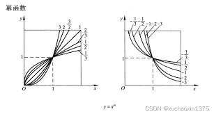
The next few pages contain a very brief survey of the basic elementary functions ${ }^{5}$ – Power, Exponential, Logarithmic, and Trigonometric Functions. If the reader is familiar with that material, she can safely skip it and go to the next lecture. However, we know from the experience that many students, especially at the community colleges, know (if any) this stuff insufficiently, that is why it is included here.
Consider a quadratic equation $x^{2}=3$. It has two real roots, $\pm \sqrt{3}$. A similar equation $x^{2}=-3$ has no real solution, but if we consider it over the larger set of complex numbers, the equation has two roots. The reason for that is that the map $y=x^{2}$ for real $x$ is not a surjection, that is, given a $y$, we not always can return to $x$. This is a very common problem, and we address it now.
First, we consider bijective maps and let $f: X \rightarrow Y$ be bijective. This means that for every element $y \in Y$ there exists one and only one element $x=x_{y} \in X$ such that $y=f(x)$. Now we construct the map $g: Y \rightarrow X$ as follows. For every $y \in Y$ we set $g(y)=x_{y}$, where $x_{y}$ has been just defined. Since the element $y_{x}$ was defined uniquely, we uniquely defined the map $g: Y \rightarrow X$. By our construction, the map $g$ has the following properties. The domain of $g$ is $Y$ and the co-domain is $X$. For each $x \in X$,$g \circ f(x)=g(f(x))=g(y)=x$ and $f \circ g(y)=f(g(y))=f\left(x_{y}\right)=y$, therefore, $$ g \circ f=I_{X} \text { and } f \circ g=I_{\gamma} . $$
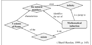
数学代写|离散数学作业代写discrete mathematics代考|The Axiom of Mathematical Induction
The Axiom of Mathematical Induction in equivalent form. Let $S$ be some set of natural numbers. Let $0 \in S$ and if some natural number $k \in S$, then also the following natural number $k+1 \in S$. Then $S$ is the set of all natural numbers ${0,1,2, \ldots}$.
Problem 8 Prove that in every problem above one can apply any of the equivalent forms of the axiom of induction.
Problem 9 Prove that $n-3$ diagonals divide an $n$ – gon, that is, the polygon with $n$ sides (not necessarily convex) into $n-2$ parts.
Proof. It is convenient in this problem to start at $n=3$. Thus, a polygon is a triangle, which has no diagonal, and consists of $3-2=1$ part, that establishes the basis of induction. Now assume that for all the $k-$ gons the statement is true, and consider any polygon $P$ with $k+l$ sides. Any its diagonal $d$ splits $P$ into two smaller polygons with a $k_{1}$ and a $k_{2}$ sides, respectively, where $k_{1}+k_{2}$ counts $d$ twice. Thus, $k_{1}+k_{2}=k+1-1=k$. On the other hand, the total number of parts is $k_{1}-1+k_{2}-1+1=k_{1}+k_{2}-1=k-1=(k+1)-2$. The following example shows that the induction can be employed to prove inequalities as well. Problem 10 Prove that $\frac{1}{\sqrt{1}}+\frac{1}{\sqrt{2}}+\frac{1}{\sqrt{3}}+\cdots+\frac{1}{\sqrt{n}}>\sqrt{n}$. Problem 11 The next is called The Strong Mathematical Induction Principle. Let $S$ be some set of natural numbers and $0 \in S$. Moreover, if for any natural number $k$, the natural numbers $0,1,2, \ldots, k-1, k \in S$, then also the following natural number $k+1 \in S$. Then $S$ is the set of all natural numbers ${0,1,2, \ldots}$. The assumptions here seem to be stronger than in the standard principle above, since we assume something not only about $k$, but also about all smaller natural numbers $j \leq k$. Thus the statement looks weaker. But both principles are equivalent.
Indeed, prove that the Strong Principle of Mathematical Induction is equivalen to the Principle of Mulheтulical Induction in stundurl form. The natural numbers satisfy the Axiom of Mathematical Induction. Moreover, they have a more general property, the Well-Ordering Principle; it considered in more detail, for example, in [31, p. 20].
数学代写|离散数学作业代写discrete mathematics代考|FACTORIALS AND THE STIRLING FORMULA
In the previous computation, we had to multiply consecutive natural numbers. This procedure occurs so often that it deserved its own name and symbol.
Definition 2 The product of $n$ consecutive natural numbers from 1 through $n$ inclusive is called the $n$ factorial and is denoted as $n !$.
For example, $1 !=1,2 !=2 \times 1=2,3 !=3 \times 2 \times 1=6$; if $k<n$, then $\frac{n !}{k !}=(k+1)(k+2) \cdots n$. If we want to preserve this property for $k=0$, it is natural to define $0 !=1$.
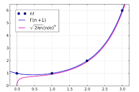
The symbol $n$ ! does not look very impressive for small $n$ but let us study it more carefully. Already $10 !=3,628,800$, and we observe that the factorials grow very fast. James Stirling (1692-1770), the younger contemporary of Newton (1643-1727), showed the asymptotic formula to be proved in Lemma 2, $$ n ! \approx\left(\frac{n}{e}\right)^{n} \sqrt{2 \pi n}, n \rightarrow \infty $$ The letter $e$ is a standard symbol for the famous real number $e \approx 2.7$, which will be discussed below. The symbol $\approx$ and name here mean that the ratio of the left- and right-hand sides of the formula tend to 1 as $n \rightarrow \infty$. This formula, without the precise value of the constant, was known to Abraham de Moivre (1667-1754) even before Stirling.
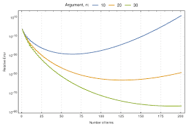
Problem 12 Approximate 10 ! by formula (1.4) and compare with the exact value given above.
Solution. By Stirling’s formula, $10 ! \approx 3.6 \times 10^{6}$, with the relative error less than $1 \%$. If $n$ is increasing, the relative error is even smaller.
Problem 13 Compute $\frac{(n+1) !}{(n-1) !}$. For what natural numbers is this expression defined? Solution. For $n-1 \geq 0$, hence $n \geq 1$. Problem 14 How many digits are in the number $100 !$ ?
The Principle, or Axiom, or Postulate of Mathematical Induction, is one of the cornerstones of any mathematical reasoning and, in particular, of our course. It is claimed that the outstanding mathematician Leopold Kronecker (1823-1891) said that “God created natural numbers, all else is humans’ business.” As with any trivial truth, it can be wrong. Indeed, many thousand years ago, together with learning to talk, people started to count, and eventually, the names for small numbers had appeared, like “one,” “two,” “three,” etc., different for various languages. Moreover, we know, for example, from observations of Russian ethnographer and traveler Nikolas Miklukho-Maklai (1846-1888) over the indigenous people of Papua-New Guinea, that people had initially developed several specialized versions of the word “one,” such that the phrase “one tree” sounded initially differently than “one boat,” or than “one kid.” Only gradually, during millennia, those various versions of “one something” merged in the abstract word “one,” which means the natural number without any specific meaning attached.
During the centuries, arithmetic has been developed together with the human society, and now there is the highly sophisticated mathematical discipline, the Number Theory, which studies, in particular, the properties of the natural numbers ${ }^{1}{0,1,2,3, \ldots}$, of the (positive, negative, and zero) integers ${\ldots,-3,-2,-1,0,1,2,3,4, \ldots}$, of the prime numbers, etc. We accept as the known facts that the natural numbers and the integers satisfy the four standard arithmetic operations. In particular, if any three integers are connected as $a=b \times c$, which can be written as $a=b \cdot c$, then the integers $b$ and $c$ are called factors or multipliers, and $a$ is called the product. If we rewrite the equation as $a \div b=c$, then $a$ is called the dividend, $b$ the divisor, and $c$ the quotient. It is also said that $b$ (and $c$ as well) divides $a$, or that $a$ is divisible by $b$ and by $c$, or that $b($ and $c)$ divides into $a$.
数学代写|离散数学作业代写discrete mathematics代考|The Axiom of Mathematical Induction
The Axiom of Mathematical Induction. Consider a set of statements, maybe formulas $S_{n_{1}}, S_{n_{1}+1}, S_{n_{1}+2}, \ldots$, numbered by all sufficiently large integers $n \geq n_{1}$. Usually $n_{1}=1$ or $n_{1}=0$, but it can be any integer. The statement $S_{n}$ is called the Induction Hypothesis or Inductive Assumption. (1) First, suppose that the statement $S_{n_{1}}$, called the basis step of induction, or just the base is valid. In applications of the method of mathematical induction, the verification of the basic step is an independent problem. In some problems, this step may be trivial, but it can never be skipped altogether. (2) Second, suppose that for each integer $n \geq n_{1}$, that is, bigger than or equal to the basis value, we can prove a conditional statement $S_{n} \Rightarrow S_{n+1}$, that is, we can prove the validity of the hypothesis $S_{n+1}$ for each specified natural $n>n_{1}$ assuming the validity of $S_{n}$, and this conditional statement is valid for all natural $n \geq n_{1}$. This part of the method is called the inductive step. (3) If we can independently show these two steps, then the Principle of Mathematical Induction claims that all infinitely many of the statements $S_{n}$, for all integer $n \geq n_{1}$ are valid.
This method of proof is accepted as an axiom because nobody can actually verify infinitely many statements $S_{n}, n \geq n_{1}$; the method cannot be justified without using some other, maybe even less intuitively obvious, properties of the set of natural numbers. Mathematicians have been using this principle for centuries and never arrived at a contradiction. Therefore, we accept the method of mathematical induction without a proof, as a postulate, and believe that this principle properly expresses a certain fundamental property of the infinite set $\mathcal{N}$ of natural numbers.
The first result we present holds definitionally and is useful for translating between results couched in typical Ramsey theory language and results given in standard graph theory language. Letting $G$ be any graph, we interpret it as a 2-coloring of the edges of $K_{|G|}$ by coloring all edges in $G$ red and the remaining edges (not present in $G$ ) blue. This coloring has no red $K_{\omega(G)+1}$ and no blue $K_{\alpha(G)+1}$ by definition. This yields the following result.
Lemma 3.15. Let $G$ be any graph. Then $R(\omega(G)+1, \alpha(G)+1) \geq|G|+1$.
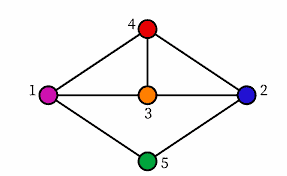
Applying Lemma $3.15$ with $G$ being a 5 -cycle we easily have $\omega(G)=2$ and $\alpha(G)=2$ so that $R(3,3) \geq 6$, which as we have seen is tight.
The next general result is a special case of a result of Chvátal and Harary [46]. We remind the reader that all arbitrary graphs we consider are connected. Theorem 3.16. Let $G$ and $H$ be graphs. Then $$ R(G, H) \geq(\chi(G)-1)(|H|-1)+1 . $$ Proof. Let $$ n=(\chi(G)-1)(|H|-1) $$ We will exhibit a 2-coloring of the edges of $K_{n}$ with no red $G$ and no blue $H$, from which the inequality follows. Partition the vertices of $K_{n}$ into $\chi(G)-1$ parts of $|H|-1$ vertices each. In each part, color all edges between the $|H|-1$ vertices blue. Color the remaining edges of $K_{n}$ red. Hence, every edge between copies of $K_{|H|-1}$ is red. Clearly this coloring admits no blue $H$ as $H$ cannot be a subgraph of $K_{|H|-1}$. We must show that there is no red $G$.
Assume, for a contradiction, that this coloring admits a red $G$. Then $G$ may have at most one vertex in each copy of $K_{|H|-1}$. Hence, $G$ can have at most $\chi(G)-1$ vertices. However, this means we can use $\chi(G)-1$ colors to color the vertices of $G$ to produce a vertex-valid coloring of $G$. This contradicts the definition of $\chi(G)$ as being the minimal such number.
Applying Theorem 3.16, we give our first result for specific types of graphs. This result is due to Chvátal [45]. Recall that $T_{m}$ is a tree on $m$ vertices. Corollary 3.17. Let $m, n \in \mathbb{Z}^{+}$. For any given tree $T_{m}$, we have $$ R\left(T_{m}, K_{n}\right)=(m-1)(n-1)+1 . $$ Proof. Using $G=K_{n}$ and $H=T_{m}$ in Theorem $3.16$ we immediately have $R\left(T_{m}, K_{n}\right) \geq(m-1)(n-1)+1$ so it remains to show that $R\left(T_{m}, K_{n}\right) \leq$ $(m-1)(n-1)+1$. To show this we induct on $m+n$, with $R\left(T_{2}, K_{n}\right)=n$ and $R\left(T_{m}, K_{2}\right)=m$ being trivial. Note that the inductive assumption means the formula holds for any type of tree on less than $m$ vertices. Let $K$ be the complete graph on vertices $V$ with $$ |V|=(m-1)(n-1)+1 . $$
数学代写|离散数学作业代写discrete mathematics代考|Hypergraphs
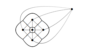
Describing the die in Figure $3.5$ as a graph on 8 vertices, our edge set would be $$ {{a, b},{a, d},{a, e},{b, c},{b, f},{c, d},{c, g},{d, h},{e, f},{e, h},{f, g},{g, h}} . $$ But this is not how we would normally describe a standard die. We typically note the 6 sides of a die and not the edges as we have given them. We may
call the sides faces; however, in order to abstract the idea of a graph, let’s call them some type of edge. For the same reason we abstract a plane in 3 dimensions to a hyperplane in more than 3 dimensions, we abstract edges of more than 2 vertices to hyperedges.
Recalling Definition 3.1, we may refer to the faces of our cube as hyperedges and describe the associated hypergraph as being on the vertices $a, b, c, d, e, f, g, h$ with hyperedge set $$ {{a, b, c, d},{a, b, e, f},{a, d, e, h},{b, c, f, g},{c, d, g, h},{e, f, g, h}} $$ The reader may notice that each hyperedge in this description contains exactly 4 vertices. This is an example of a hypergraph in the class a hypergraphs with which we will be dealing.
Definition $3.19$ ( $\ell$-uniform hypergraph). Let $G=(V, E)$ be a hypergraph. Let $\ell \in \mathbb{Z}^{+}$with $\ell \geq 3$. If every element of $E$ contains exactly $\ell$ vertices from $V$, then we say that $G$ is an $\ell$-uniform hypergraph. If $E$ contains all ( $\ell \mid$ subsets of $V$ of size $\ell$, then we call $G$ the complete $\ell$-uniform hyperyraph and denote it by $K_{n}^{\ell}$, where $n=|V|$.
Applying this definition to the die example above, our second description is one of a 4-uniform hypergraph; however, it is not a complete 4-uniform hypergraph since it has only 6 hyperedges and not all $\left(\begin{array}{l}6 \ 4\end{array}\right)=15$ hyperedges that a $K_{6}^{4}$ has.
In Ramsey’s Theorem we color edges and deduce monochromatic complete subgraphs. Replacing edges with hyperedges and subgraphs with subhypergraphs is the basis of the Hypergraph Ramsey Theorem, which is actually the original theorem proved by Ramsey in his seminal paper [166, Theorem A]. Formally, for a hypergraph $H=(V, E)$, each hyperedge in $E$ is assigned a color and a subhypergraph on vertices $U \subseteq V$ may only have a hyperedge $e \in E$ provided $e \in \wp(U)$.
Notation. We will refer to a hyperedge consisting of $\ell$ vertices as an $\ell$ hyperedge.
Theorem 3.20 (Hypergraph Ramsey Theorem). Let $\ell, r \in \mathbb{Z}^{+}$with both at least 2. For $i \in{1,2, \ldots, r}$, let $k_{i} \in \mathbb{Z}^{+}$with $k_{i} \geq \ell$. Then there exists a minimal positive integer $n=R_{\ell}\left(k_{1}, k_{2}, \ldots, k_{r}\right)$ such that every $r$-coloring of the $\ell$-hyperedges of $K_{n}^{\ell}$ with the colors $1,2, \ldots, r$ contains, for some $j \in$ ${1,2, \ldots, r}$, a $K_{k_{j}}^{\ell}$ subhypergraph with all $\ell$-hyperedges of color $j$.
Proof. We start by proving the $r=2$ case. We prove this via induction on $\ell$. The $\ell=2$ case of this theorem is Ramsey’s Theorem (Theorem $3.6$ ), so that we have already proved the base case. Given $k_{1}$ and $k_{2}$, by the inductive assumption we assume that $n=R_{\ell-1}\left(k_{1}, k_{2}\right)$ exists. For ease of exposition, we
will use the colors red and blue, with red associated with $k_{1}$ (and blue with $\left.k_{2}\right)$.
Inside of the induction on $\ell$, we induct on $k_{1}+k_{2}$, as we did in the proof of Ramsey’s Theorem. So, in our pursuit of showing that $R_{\ell}\left(k_{1}, k_{2}\right)$ exists, we may assume that $R_{\ell}\left(k_{1}-1, k_{2}\right)$ and $R_{\ell}\left(k_{1}, k_{2}-1\right)$ both exist. The base cases for our induction on $k_{1}+k_{2}$ are trivial: $R_{\ell}\left(\ell, k_{2}\right)=k_{2}$ and $R_{\ell}\left(k_{1}, \ell\right)=k_{1}$ (for the first, we either have a red hyperedge and, hence, a red $K_{\ell}^{\ell}$, or all hyperedges are blue and we have a blue $K_{k_{2}}^{\ell}$; for the second, reverse the colors and use $k_{1}$ instead of $k_{2}$ ). Hence, we may assume that $k_{1}$ and $k_{2}$ are both greater than $\ell$. Let $$ n=R_{\ell-1}\left(R_{\ell}\left(k_{1}-1, k_{2}\right), R_{\ell}\left(k_{1}, k_{2}-1\right)\right)+1 . $$ We will show that $R_{\ell}\left(k_{1}, k_{2}\right) \leq n$. Consider an arbitrary 2 -coloring $\chi$ of the $\ell$-hyperedges of $K_{n}^{\ell}$ with vertex set $V$. Isolate a vertex $v \in V$. Consider the complete $(\ell-1)$-uniform hypergraph on vertices $V \backslash{v}$ where the coloring $\widehat{\chi}$ of the $(\ell-1)$-hyperedges is inherited from $\chi$ in the following way: For $e$ an $(\ell-1)$-hyperedge, let $$ \widehat{\chi}(e)=\chi(e \cup{v}) . $$ From the definition of $n$ we have either a complete $(\ell-1)$-uniform hypergraph on $R_{\ell}\left(k_{1}-1, k_{2}\right)$ vertices with all $(\ell-1)$-hyperedges red under $\hat{\chi}$ or a complete $(\ell-1)$-uniform hypergraph on $R_{\ell}\left(k_{1}, k_{2}-1\right)$ vertices with all $(\ell-1)$-hyperedges blue under $\hat{\chi}$. Without loss of generality, we may assume the latter holds.
Let $W$ be the set of $R_{\ell}\left(k_{1}, k_{2}-1\right)$ vertices with all $(\ell-1)$-hyperedges blue under $\hat{\chi}$. By the assumed existence of $R_{\ell}\left(k_{1}, k_{2}-1\right)$ we have, under $\chi$, either a red $K_{k_{1}}^{\ell}$ and are done, or we have a blue $K_{k_{2}-1}^{\ell}$ on vertex set $U$ with the property that all $(\ell-1)$ hyperedges are blue under $\widehat{\chi}$. Noting that $v \notin U$, consider the complete $\ell$-uniform hypergraph on the vertices $U \cup{v}$. The $\ell$ hyperedges that include $v$ are all blue since, by the definition of $\widehat{\chi}$, we have $\widehat{\chi}(e)=\chi(e \cup{v})$ for any $(\ell-1)$-hyperedge $e$ with vertices in $V \backslash{v}$, which we have deduced are all blue in $K_{k_{2}-1}^{\ell}$. Thus, all $\ell$-hyperedges on $U \cup{v}$ are blue and we have a blue $K_{k,}^{\ell}$. This completes the $r=2$ case of the theorem.
数学代写|离散数学作业代写discrete mathematics代考|Some Graph Theory Concepts
We start by reminding the reader of a few definitions about graphs. Definition 3.1 (Graph, Hypergraph, Degree, Edge, Hyperedge). Let $V$ be a set, called the vertices, and let $E$ be a subset of $\wp(V) \backslash \emptyset$ (the power set of $V$ excluding the empty set). We say that $G=(V, E)$ is a graph if all elements of $E$ are subsets of size 2. In this case, $E$ is referred to as the set of edges. For any given vertex $v$, the number of edges containing $v$ is called the degree of
$v$. We say that $G=(V, E)$ is a hypergraph if some element of $E$ is a subset of more than 2 elements. In this case, $E$ is called the set of hyperedges.
Definition $3.2$ (Subgraph, Subhypergraph). Let $G=(V, E)$ be a graph. If $V^{\prime} \subseteq V$ and $E^{\prime} \subseteq E$ then $H=\left(V^{\prime}, E^{\prime}\right)$ is a subgraph of $G$. If $G$ is a hypergraph, then we call $H$ a subhypergraph.
We will start by considering graphs (hypergraphs are treated later in this chapter). We will assume that any arbitrary graph we consider is connected so that there exists a string of edges from any vertex to any other vertex. We also assume that our graphs are simple, meaning that at most one edge exists between any two vertices. We will start by considering one of the fundamental graphs: the complete graph.
Definition $3.3$ (Complete graph). Let $n \in \mathbb{Z}^{+}$. The complete graph on $n$ vertices, denoted $K_{n}$, is $G=(V, E)$ where $|V|=n$ and $E$ consists of all subsets of $V$ of size 2 .
We typically identify the vertex set $V$ of $K_{n}$ with ${1,2, \ldots, n}$ and the edge set $E$ with ${{i, j}: i, j \in[1, n] ; i<j}$. In other words, all $\left(\begin{array}{c}n \ 2\end{array}\right)$ possible edges are present in a complete graph.
We start with the classical version of Ramsey’s Theorem, restricted to the 2-color situation.
Theorem 3.4. Let $k, \ell \in \mathbb{Z}^{+}$. There exists a minimal positive integer $n=$ $n(k, \ell)$ such that if each edge of $K_{n}$ is assigned one of two colors, say red and blue, then $K_{n}$ admits a complete subgraph on $k$ vertices with all edges red or a complete subgraph on $\ell$ vertices with all edges blue.
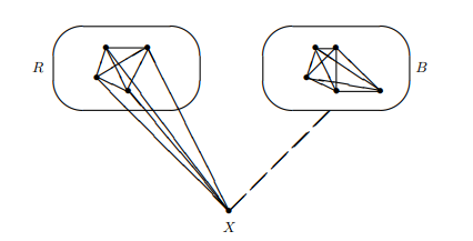
Before getting to the proof, let’s consider the $k=\ell=3$ case. We will refer to $K_{3}$ as a triangle and will show that $n(3,3) \leq 6$. Consider any 2-coloring of the edges of $K_{6}$. Isolate one vertex; call it $X$. Then $X$ is connected to the other 5 vertices with either a red or a blue edge. Let $R$ be the set of vertices connected to $X$ with a red edge; let $B$ be the set of vertices connected to $X$ with a blue edge. We know that $|R \cup B|=5$ and that $R \cap B=\emptyset$. Hence, $|R \sqcup B|=|R|+|B|=5$. From this we can conclude by the pigeonhole principle that either $|R| \geq 3$ or $|B| \geq 3$. Without loss of generality, we assume $|R| \geq 3$. At this stage we have $X$ connected to at least 3 vertices, call them $A, B$, and $C$, via red edges. Consider the edges between these latter 3 vertices. If any edge is red, say ${A, B}$, then we have a red triangle (on vertices $A, B$, and $X)$. In other words, we have deduced a $K_{3}$ with all edges red. On the other hand, if no edge is red, then they are all blue and we can conclude that the triangle on vertices $A, B$, and $C$ has all blue edges, i.e., we have a $K_{3}$ with all blue edges.
The proof for general $k$ and $\ell$ follows the same idea as the case for $k=\ell=$ 3 . We will isolate one vertex and separate the other vertices according to the color of the edge to the isolated vertex.
As our first “application” of Ramsey’s Theorem, we will deduce Schur’s Theorem. Recall that Schur’s Theorem states that there exists a minimal positive integer $s(r)$ such that every $r$-coloring of $[1, s(r)]$ admits a monochromatic solution to $x+y=z$. So, we need to deduce integer solutions from a graph. We do so by considering a subclass of colorings of $K_{n}$.
Definition 3.7 (Difference coloring). A difference coloring of the edges of $K_{n}$ is one in which the color of every edge ${i, j}$ depends solely on $|i-j|$.
With this definition, if $\chi:[1, n-1] \rightarrow{0,1, \ldots, r-1}$ is a coloring of integers, then we have the induced difference coloring of $K_{n}$ where we color edge ${i, j}$ with $\chi(|i-j|)$.
To deduce Schur’s Theorem, let $n=R(3 ; r)$. For any $r$-coloring of $[1, n-1]$ consider the difference coloring of the edges of $K_{n}$. By Ramsey’s Theorem, this difference coloring admits a monochromatic $K_{3}$, say on the vertices $u, v$, and $w$, with $u<v<w$. This means that the integers $v-u, w-v$, and $w-u$ all have the same color. Let $x=v-u, y=w-v$, and $z=w-u$ to see that we have a solution to $x+y=z$ with $x, y$, and $z$ all the same color. Consequently, we see that $s(r) \leq R(3 ; r)-1$.
The above argument can be easily extended to show that any $r$-coloring of the integer interval [1, R( $k ; r)-1]$ admits a monochromatic solution to $\sum_{i=1}^{k-1} x_{i}=x_{k}$. The minimal positive integer $n=n(k ; r)$ such that every $r-$ coloring of $[1, n]$ admits a monochromatic solution to $\sum_{i=1}^{k-1} x_{i}=x_{k}$ is referred to as a generalized Schur number. This argument gives $n(k ; r) \leq R(k ; r)-1$. It is known [21] that $$ n(k ; 2)=k^{2}-k-1 $$ however, $n(k ; r)$ for $r \geq 3$ is unknown: the bound $$ n(k ; r) \geq \frac{k^{r+1}-2 k^{r}+1}{k-1} $$has been determined [21]. As we can see, the bound between these two Ramsey-type numbers is quite weak since we have seen that $(\sqrt{2})^{k}<R(k, k)$ (see Inequality (3.1)) so that the $k^{2}-k$ lower bound on $R(k, k)$ is not strong. The reason for this is because we do not use the whole complete monochromatic subgraph in deducing the existence of $n(k ; r)$.
数学代写|离散数学作业代写discrete mathematics代考|Other Graphs
As stated at the end of the last section, the proof that generalized Schur numbers exist as a consequence of Ramsey’s Theorem does not use the full power of Ramsey’s Theorem. In particular, we do not need a monochromatic complete graph; we only need the “outside” edges of this complete graph to have the same color, i.e., a monochromatic cycle.
Definition $3.8$ (Path, Cycle, Tree). Let $G=(V, E)$ be the graph with vertex set $V=\left{v_{1}, v_{2}, \ldots, v_{n}\right}$ and edge set $E=\left{\left{v_{i}, v_{i+1}\right}: i \in{1,2, \ldots, n-1}\right}$. Then $G$ is called a path (from $v_{1}$ to $v_{n}$, or $v_{n}$ to $v_{1}$ ) and we denote it by $P_{n}$. If we add the edge $\left{v_{1}, v_{n}\right}$ to the edge set, then $G$ is called an $n$-cycle and we denote it by $C_{n}$. Paths are a subclass of the class of graphs known as trees. A tree $T_{n}$ is a graph on $n$ vertices with no $k$-cycle as a subgraph, for any $k$. There are many other named graphs (for example, in Figure $3.2$ we present a graph attributed to Kempe but commonly referred to as the Peterson graph. which is useful as it often serves as a counterexample). Complete graphs, paths, cycles, and trees are some of the important ones. Below we define two more important classes of graphs.
数学代写|离散数学作业代写discrete mathematics代考|Graph Ramsey Theory
Notation. In this subsection, $i$ is reserved for $i=\sqrt{-1}$ and for $c \in \mathbb{C}$ we use $\bar{c}$ to represent the complex conjugate.
We will be doing analysis over the group $\left(\mathbb{Z}{n,}+\right):$ for $f: \mathbb{Z}{n} \rightarrow \mathbb{C}$, let the (discrete) Fourier transform of $f$ be denoted by $\hat{f}$ and given by (for $t \in \mathbb{Z}{n}$ ): $$ \widehat{f}(t)=\frac{1}{n} \sum{k=0}^{n-1} f(k) \overline{\chi(k t)} $$
Instead of appealing to van der Waerden’s Theorem as was done in the proof of Theorem 2.67, our goal is now to prove arithmetic progressions exist in certain sets. We start with the simplest case to consider: 3 -term arithmetic progressions. This does not mean that the result concerning these is easy to prove. In 1952 , Roth $[174]$ proved that any subset of $\mathbb{Z}^{+}$with positive upper density must contain a 3 -term arithmetic progression. Note that since every finite coloring of $\mathbb{Z}+$ must have at least one color with positive upper density, Roth’s Theorem is stronger than the existence of $w(3 ; r)$ for all $r \in \mathbb{Z}^{+}$.
Theorem $2.68$ (Roth’s Theorem). For any $\epsilon>0$, there exists $N=N(\epsilon)$ such that for any $n \geq N$, if $A \subseteq[1, n]$ with $|A|>\epsilon n$, then $A$ contains a S-term arithmetic progression. Remark. Another way of stating Roth’s Theorem is: $r_{3}(n)=o(n)$. Since we are dealing with 3 -term arithmetic progressions, we can consider integer solutions to $x+y=2 z$, where $x, y$, and $z$ are not all equal. To effectively use discrete Fourier analysis, instead of looking for solutions in $\mathbb{Z}^{+}$, we will be looking at solutions in $\mathbb{Z}_{n}$, so we are considering solutions to $x+y \equiv 2 z$ $\left(\bmod n\right.$ ). A simple observation will allow us to translate back to $\mathbb{Z}^{+}$.
The general approach of the proof is to consider cases depending on the sizes of the Fourier transform coefficients. It is best to have a little intuition into what these mean. Consider the recovery formula given in part (i) of Theorem 1.9: $$ \begin{aligned} f(j) &=\sum_{k=0}^{n-1} \widehat{f}(k) \chi(k j) \ &=\sum_{k=0}^{n-1} \widehat{f}(k) e^{\frac{2 \pi i k j}{n}} \ &=\sum_{k=0}^{n-1} \widehat{f}(k) \cos \left(\frac{2 \pi k j}{n}\right)+i \sum_{k=0}^{n-1} \widehat{f}(k) \sin \left(\frac{2 \pi k j}{n}\right) \ &=\widehat{f}(0)+\sum_{k=1}^{n-1} \widehat{f}(k) \cos \left(\frac{2 \pi k j}{n}\right)+i \sum_{k=1}^{n-1} \widehat{f}(k) \sin \left(\frac{2 \pi k j}{n}\right) \cdot(2.9) \end{aligned} $$ The first observation is that $\widehat{f}(0)$ is a constant term in $f(j)$, while the other values of $\hat{f}(k)$ are contracted by a factor depending on $j$. To guide our intuition, we then couple this with the fact that any periodic function over $\mathbb{R}$ (like $\cos (x)$ ) has roots in arithmetic progression (not necessarily of integers). First, we need to recall how we translate from a set $A \subseteq[1, n]$ to a function $f: \mathbb{Z}_{n} \rightarrow \mathbb{C}$ by using the indicator function: $$ A(j)= \begin{cases}1 & \text { if } j \in A \ 0 & \text { if } j \notin A\end{cases} $$
Translating the proof of Roth’s Theorem to address longer arithmetic progressions presents the challenge of moving from solving the equation $x+y=2 z$ to solving a system of equations. Clearly, more sophisticated Fourier analysis tools are needed and this was done twenty years later by Roth $[175]$ for 4 -term arithmetic progressions. However, this was after Szemerédi [195] proved the result via combinatorial methods. Szemerédi then went on to prove his famous theorem for arbitrarily long arithmetic progressions in [196]:
Theorem 2.70 (Szemerédi’s Theorem). For any $k \in \mathbb{Z}^{+}$and any subset $A \subseteq \mathbb{Z}^{+}$, if limsup $\operatorname{sun}_{n \rightarrow \infty} \frac{|A \cap[1, n]|}{n}>0$, then A contains a $k$-term arithmetic progression. Equivalently, given $\epsilon>0$ there exists an integer $N(k, \epsilon)$ such that for all $n>N(k, \epsilon)$, if $|A|>\epsilon n$, then $A$ contains a $k$-term arithmetic progression.
Szemerédi’s proof has been referred to as elementary. This does not mean easy. It is better referred to as “from first principles,” as Szemerédi felt just the logic of the proof warranted a flow chart. This chart is a directed graph on 24 vertices with 36 edges.
The reader is encouraged to work through this combinatorial feat. In this book, we prove Szemerédi’s Theorem in Section 5.2.1, relying on results that we will not prove.
It is worth noting here that Szemerédi’s Theorem is equivalent, by Theorem $2.67$, to the following theorem, the proof of the equivalence being left to the reader as Exercise $2.23$. Note also that Theorem $2.70$ settles the value of $L$ in Theorem 2.67.
Theorem 2.71. For all $k \in \mathbb{Z}^{+}$, there exists a minimal integer $N(k)$ such that for every partition of ${1,2, \ldots, n}=A \sqcup B$ with $|A| \geq|B|$ and $n \geq N(k)$, the set $A$ contains a $k$-term arithmetic progression.
It is interesting to notice that van der Waerden’s Theorem can be very similarly stated as: For all $k \in \mathbb{Z}^{+}$, there exists a minimal integer $M(k)$ such that for every partition of ${1,2, \ldots, m}=A \sqcup B$ with $m \geq M(k)$, one of $A$ and $B$ contains a $k$-term arithmetic progression.
In this section, we will investigate a closely related result that, on the surface, seems as if it may be sufficient to prove Szemerédi’s Theorem. One possible thought about sets satisfying the condition in Theorem $2.70$ is that they cannot have arbitrarily long gaps (forewarning: this is not true) or, if they do, then there must be arbitrarily long intervals where they don’t (forewarning: this is not true either). These seem reasonable, so we will investigate what we can say about this situation.
Definition $2.72$ (Syndetic, Piecewise syndetic). Let $S=\left{s_{i}\right}_{i \in Z^{+}}$. We say that $S$ is syndetic if there exists $d \in \mathbb{Z}^{+}$such that $\left|s_{i+1}-s_{i}\right| \leq d$ for all $i \in \mathbb{Z}^{+}$. We say that $S$ is piecewise syndetic if there exists $d \in \mathbb{Z}^{+}$such that for any $n \in \mathbb{Z}^{+}$, there exists $j \in \mathbb{Z}^{+}$such that $\left|s_{i+1}-s_{i}\right| \leq d$ for $i=j, j+1, \ldots, j+n-1$.
We start with the statement of the theorem in this subsection’s title: Theorem 2.74 (Density Hales-Jewett Theorem). Let $\epsilon>0$ and let $k, r \in$ $\mathbb{Z}^{+}$. Let $\mathcal{W}(m)$ be the set of all variable words of length $m$ over the alphabet ${1,2, \ldots, k} \cup{x}$. There exists an integer $N=N(\epsilon, k)$ such that for any $n \geq N$, every subset $S \subseteq[1, k]^{n}$ with $|S|>\epsilon k^{n}$ admits $w(x) \in \mathcal{W}(n)$ with ${w(i): i \in[1, k]} \subseteq S .$
This result was originally proved by Furstenberg and Katznelson [77] using ergodic theory (see Section $5.2$ for an introduction to ergodic theory techniques). Over 30 years later a combinatorial proof was developed [160]. Needless to say, both proofs are very deep and are not appropriate for this
book. For a good exposition of Theorem 2.74, visit the last chapter of [161] (written by Steger; see the Foreword of [161]).
We remark that the $k=2$ case follows by viewing $x_{1} x_{2} \cdots x_{n} \in[1,2]^{n}$ as the subset of $[1, n]$ containing $i$ if and only if $x_{i}=2$. Consider the lattice of $[1,2]^{n}$ partially ordered by inclusion of the associated subsets, i.e., an edge connects two subsets if one is a subset of the other. We are searching for $w(x) \in \mathcal{W}(n)$ such that $w(1)$ and $w(2)$ are both in $S$. This means that we are looking for two subsets connected by an edge.
Recall the concept of an antichain in a poset. An antichain is a set of elements in the lattice with no edge between any of them. A fundamental poset result is Sperner’s Lemma, which states that every antichain of the subsets of $[1, n]$ under inclusion partial ordering has size at most $$ \left(\begin{array}{c} n \ \left\lfloor\frac{n}{2}\right\rfloor \end{array}\right)=\frac{n !}{\left\lfloor\frac{n}{2}\right\rfloor^{2}} \approx \frac{\sqrt{2 \pi n}\left(\frac{n}{e}\right)^{n}}{\pi n\left(\frac{n / 2}{e}\right)^{n}}=\frac{2^{n}}{\sqrt{\frac{\pi}{2} n}}=o\left(2^{n}\right) $$ where we are using Stirling’s approximation. Lastly, note that if our set $S$ has $|S| \geq \epsilon \cdot 2^{n}$, then $S$ cannot be an antichain since it contains more than $o\left(2^{n}\right)$ elements. Hence, $S$ must contain two elements with an edge between them, which is what we want to show.
The result named in this subsection is a mouthful. This stems from the independent, and distinct, proofs used to prove the result that all occurred around the same time. From historical research done by Soifer [191] we find that Arnautov in [9], Folkman via personal communication, and Sanders in [178], all proved the same result, which is a generalization of Schur’s Theorem. As noted in [84], the result also follows directly from Rado’s Theorem (hence the inclusion of Rado’s name). We will offer two different proofs in this subsection: one based on van der Waerden’s Theorem (due to Folkman) and one based on Rado’s Theorem. A third proof will be given in Section 3.3.2 as it appeals to a result presented in the next chapter. Other (different) proofs can be found in $[152,199]$.
Theorem 2.55 (Arnautov-Folkman-Rado-Sanders’ Theorem). Let $k, r \in \mathbb{Z}^{+}$. There exists a minimal positive integer $n=n(k ; r)$ such that every $r$-coloring of $[1, n]$ admits $S \subseteq[1, n]$ with $|S|=k$ such that $F S(S)$ is monochromatic. Proof based on van der Waerden’s Theorem. We start by defining the auxiliary function $a=a(k ; r)$ as the minimal positive integer such that every $r$-coloring of $[1, a]$ admits $B=\left{b_{1}<b_{2}<\cdots<b_{k}\right}$ with $F S(B) \subseteq[1, a]$ such that $$ \chi\left(b_{i_{1}}+b_{i_{2}}+\cdots+b_{i_{j}}\right)=\chi\left(b_{i_{j}}\right) $$ for any $j \in[1, k]$ with $i_{1}<i_{2}<\cdots<i_{j}$. Assume for the moment that $a(k ; r)$ exists for all $k, r \in \mathbb{Z}^{+}$. Then, by considering $a(r(k-1)+1 ; r)$, we have $B=\left{b_{1}<b_{2}<\cdots<b_{r(k-1)+1}\right}$. By the pigeonhole principle, there must be at least $k$ elements of $B$ of the same color. Say $S=\left{b_{i_{1}}, b_{i_{2}}, \cdots, b_{i_{k}}\right}$ is monochromatic. Since $F S(S) \subseteq F S(B)$ we see that every element of $F S(S)$ is colored by the largest element of the sum. Since this largest element is necessarily in $S$, and since $S$ is monochromatic, we see that $F S(S)$ is monochromatic.
So, we will be done once we establish the existence of $a(k ; r)$. We proceed by induction on $k$, with $k=1$ being trivial. Hence, let $\ell=a(k-1 ; r)$ and let
$m=w(\ell+1 ; r)$. We will show that $a(k ; r) \leq 2 m$. To this end, consider any $r$-coloring of $[1,2 m]$. By van der Waerden’s Theorem, there exist $$ c, c+d, \ldots, c+\ell d \in[m+1,2 m] $$ all the same color. Note that $c>m$. Since sumsets are closed under dilation, we can apply the inductive assumption to $d[1, \ell]$ to obtain $$ B=\left{d b_{1}m$. Let $b_{k}=c$ and notice that $d b_{k-1}<b_{k}$. As every element of $F S(B)$ is a multiple of $d$, with largest possible multiple $d \ell$ (the sum of all elements of $B$ must remain in $d[1, \ell]$ by definition of $a(k-1 ; r)$; otherwise elements larger than $a(k-1 ; r)$ would not be assigned a color $)$. Hence, if $s \in F S(B)$ we see that $s+b_{k}=c+j d$ for some $j \in[1, \ell]$. Since all members of $c+d, \ldots, c+\ell d$ are the same color as $c=b_{k}$, we have $a(k ; r) \leq 2 m$.
Proof based on Rado’s Theorem. Consider the following system of linear homogeneous equations: $$ \left{\sum_{i \in I} x_{i}=y_{I}: 0 \neq I \subseteq[1, k]\right}, $$ where we index the $y$ ‘s by the subset over which we are summing. By showing a monochromatic solution to this system exists we will have values of the variables for which $F S\left(x_{1}, x_{2}, \ldots, x_{k}\right)$ is monochromatic. By Rado’s Theorem we will be done once we show that the associated coefficient matrix satisfies the columns condition.
We are still investigating finite sums $F S(S)$; however, we will now be considering the situation when $S$ is infinite. In particular, does the conclusion of Theorem $2.55$ hold when $S$ is infinite? As you may suspect if you read the title of this subsection, an answer was achieved by Hindman [109].
Theorem $2.56$ (Hindman’s Theorem). Let $r \in \mathbb{Z}^{+}$. Every $r$-coloring of $\mathbb{Z}^{+}$ admits an infinite set $A \subseteq \mathbb{Z}^{+}$such that $F S(A)$ is monochromatic.
The proof of this must be fundamentally different than the proof when $S$ is finite. We can use neither van der Waerden’s Theorem nor Rado’s Theorem as these will only give us arbitrarily large – not infinite – sets, since both are results about finite structures.
The proof of Hindman’s Theorem is quite involved, so we will break it up into several lemmas before putting the pieces together. We will follow the proof given by Baumgartner [11]. But first, a definition is in order.
Definition $2.57$ (Disjoint sumset of $S$ ). Let $S, T \subseteq \mathbb{Z}^{+}$be infinite sets. We say $T \subseteq F S(S)$ is a disjoint sumset of $S$, and write $T \in \mathcal{D S}(S)$, if every element of $S$ is contained in at most one sum/element in $T$, where $\mathcal{D} S(S)$ is the class of all disjoint sumsets of $S$.
The benefit of this class of finite sums is that if $t_{1}, t_{2} \in T \in \mathcal{D S}(S)$ then $t_{1}+t_{2} \in F S(S)$ since the elements from $S$ used in $t_{1}$ are distinct from those used in $t_{2}$. Using this idea, we immediately have the following lemma, the proof of which is left to the reader as Exercise 2.17.
Lemma 2.58. Let $S, T, U \subseteq \mathbb{Z}^{+}$be infinite sets with $T \in \mathcal{D S}(S)$ and $U \in$ $\mathcal{D} S(T)$. Then (i) $F S(T) \subseteq F S(S)$; and (ii) $U \in \mathcal{D S}(S)$. Before the next lemma, we require another definition. Definition $2.59$ (Intersective for $S$ ). Let $S \subseteq \mathbb{Z}^{+}$be infinite. We say that a set $X$ is intersective for $S$ if for all $T \in \mathcal{D S}(S)$ we have $F S(T) \cap X \neq \emptyset$. A crucial observation here is that any intersective set must be infinite. This can be confirmed by part (ii) of the next lemma. Lemma 2.60. Let $X, S$ be subsets of $\mathbb{Z}^{+}$. The following hold: (i) Let $n \in \mathbb{Z}^{+}$and assume $X=\bigsqcup_{i=1}^{n} X_{i} .$ If $X$ is intersective for $S$, then there exists $T \in \mathcal{D S}(S)$ and $i \in{1,2, \ldots, n}$ such that $X_{i}$ is intersective for $T$. (ii) If $F$ is a finite subset of $\mathbb{Z}^{+}$and $X$ is intersective for $S$, then $X \backslash F$ is intersective for $S$.
We end this chapter by presenting some analytic approaches to integer Ramsey theory. We will mainly be considering arithmetic progressions. The standard notation used for density results concerning van der Waerden’s Theorem is given next.
Notation. For $k, n \in \mathbb{Z}^{+}$denote by $r_{k}(n)$ the maximal size of a subset of $[1, n]$ with no $k$-term arithmetic progression.
We start with a result due to Behrend $[14]$ that seems to have been overlooked. This was communicated to the author by Tom Brown. Behrend’s result appeared just a year after Erdös and Turán [71] defined $r_{3}(n)$ and showed that $$ \frac{r_{3}(n)}{n}<\frac{3}{8}+o(1) $$
Behrend’s result is more sweeping. Theorem 2.67. For each $k \in Z^{+}$we have that $$ L_{k}=\lim {n \rightarrow \infty} \frac{r{k}(n)}{n} $$ exists and, more importantly, $$ L=\lim {k \rightarrow \infty} L{k} \in{0,1} $$ Proof. The fact that $L_{k}$ exists is standard and left to the reader as Exercise 2.22. The fact that $L$ exists follows from $0 \leq L_{1} \leq L_{2} \leq \cdots \leq L_{k} \leq \cdots \leq 1$, which is a monotonic infinite sequence on a closed interval. Thus, we need only show that $L$ is either 0 or 1 . We will first show that, for every $n \in \mathbb{Z}^{+}$, we have $$ \frac{r_{k}(n)}{n}>L_{k} $$ Assume, for a contradiction, that there exists $m \in \mathbb{Z}^{+}$such that Inequality $(2.3)$ is false for $m$. We may assume that for all $n \in \mathbb{Z}^{+}$we have $$ \frac{r_{k}(m)}{m} \leq \frac{r_{k}(n)}{n} $$ We next note that $r_{k}(m n) \leq n r_{k}(m)$ since if $S \subseteq[1, m n]$ avoids $k$-term arithmetic progressions, then it is necessary (but not sufficient) that each of the intervals $[1, m],[m+1,2 m], \ldots,[(n-1) m+1, n m]$ contains at most $r_{k}(m)$ integers from $S$. From Inequality $(2.4)$ and this observation, we have $$ \frac{r_{k}(m)}{m} \leq \frac{r_{k}(m n)}{m n} \leq \frac{n r_{k}(m)}{m n}=\frac{r_{k}(m)}{m} $$ and we conclude that $r_{k}(m n)=n r_{k}(m)$ for all $n \in \mathbb{Z}+$. Define the intervals $$ A_{i}=[(i-1) m+1, i m], \quad i=1,2, \ldots, w\left(k ; 2^{m}\right) $$ where $w\left(k ; 2^{m}\right)$ is the van der Waerden number. Consider $$ n=w\left(k ; 2^{m}\right) $$
Thanks to Rado, we have a complete understanding of which systems of linear equations are regular. An obvious next step is the investigation of nonlinear equations.
Perhaps Pythagorean triples, i.e., solutions to $x^{2}+y^{2}=z^{2}$, pop to mind first. While this is a homogeneous equation, let’s not make the situation harder than we must. We’ll start with $x+y=z^{2}$. The following result is due to Green and Lindqvist $[88]$; we follow Pach $[156]$ for the proof of 2-regularity. Theorem 2.28. The equation $x+y=z^{2}$ is 2-regular, but not 3-regular. Proof. Of course $(x, y, z)=(2,2,2)$ is always a monochromatic solution under any coloring, so we do not allow this as a valid monochromatic solution.
We start by exhibiting a 3 -coloring of $\mathbb{Z}^{+}$with no monochromatic solution. Define the intervals $$ I_{j}=\left{i \in \mathbb{Z}^{+}: 2^{j} \leq i \leq 2^{j+1}-1\right} \quad \text { for } \quad j=0,1,2, \ldots $$ Let the colors be 0,1 , and 2 . For $j=0,1$, and 2 , color all elements of $I_{j}$ by color $j$. For $j=3,4, \ldots$, in order, color all elements of $I_{j}$ with a color missing from $$ I_{\left\lfloor\frac{j}{2}\right\rfloor} \cup I_{\left\lfloor\frac{j}{2}\right\rfloor+1} . $$
Assume, for a contradiction, that $a+b=c^{2}$ with $a \leq b$ is a monochromatic solution under this coloring. For some $j$ we have $b \in I_{j}$. Since $a \leq b$ we have $2^{j}<a+b<2^{j+2}$ so that $2^{\frac{j}{2}}<c<2^{\frac{j}{2}+1}$. Hence, $c \in I_{\left\lfloor\frac{j}{2}\right\rfloor} \cup I_{\left\lfloor\frac{j}{2}\right\rfloor+1}$. By construction, if $j \geq 3$, this means that the color of $c$ and $b$ are different. For $j \in{0,1,2}$ we have $b<8$ so that $c \in{2,3}$. For $c=2$, the only solutions are $(a, b, c)=(1,3,2)$ and $(2,2,2)$. The first is not monochromatic and the latter is not a valid monochromatic solution. For $c=3$, the solutions are $(2,7,3),(3,6,3)$, and $(4,5,3)$, none of which are monochromatic. Hence, the equation is not 3 -regular.
We continue by showing that for $n \geq 14$, the interval $\left[n,(10 n)^{4}\right]$ admits a monochromatic solution under any 2-coloring. To this end, let $\chi$ : $\left[n,(10 n)^{4}\right] \rightarrow{-1,1}$ be an arbitrary coloring. We use the colors $-1$ and 1 instead of the more standard 0 and 1 since we will be deriving inequalities about sums of colors and sums of $-1$ s and 1 s have more easily described properties. Assume, for a contradiction, that $\chi$ does not admit a monochromatic solution. Since $(x, y, z)=\left(n^{2}, 80 n^{2}, 9 n\right)$ is a solution, we see that $\left[9 n, 80 n^{2}\right]$ cannot be entirely of one color. Hence, there exists $$ k \in\left[9 n, 80 n^{2}-1\right] $$ such that, without loss of generality, $\chi(k)=1$ and $\chi(k+1)=-1$.
Clearly $\mathbb{Z}^{+}$is closed under addition and multiplication; however, it does not contain nontrivial multiplicative or additive inverses. This is one reason that the (non-)regularity over $\mathbb{Z}^{+}$of some of the equations in the last subsection is hard to prove. If we consider fields, we will have more tools at our disposal and may be able to prove more. This does not mean the results are easy, just that we are able to bring in more algebra and number theory. We will restrict our attention to prime order fields, i.e., $\mathbb{F}_{p}$ with $p$ prime.
A word of caution: positive results over fields do not necessarily imply that the corresponding result over $Z^{+}$is true. For example, if we consider $x^{3}+y^{3}=z^{3}$, we know that there is no solution over $Z^{+}$, while it is easy to find solutions over prime-order fields $\mathbb{F}_{p}$, e.g., $3^{3}+5^{3} \equiv 4^{3}(\bmod 11)$. Note, however, if we can find that an equation is not $r$-regular over any sufficiently large prime-order fields, then we can conclude the non-regularity over $\mathbb{Z}^{+}$via the contrapositive of the Compactness Principle.
With regards to the Fermat equations, it is known [186] that for any $k \in$ $\mathbb{Z}^{+}$, for all sufficiently large primes $p$, the equation $x^{k}+y^{k}=z^{k}$ is regular over $F_{p}$, i.e., $x^{k}+y^{k} \equiv z^{k}(\bmod p)$ has a monochromatic solution with $x y z \not 0$ $(\bmod p)$ for any $r$-coloring of $\mathbb{F}_{p}$ for $p$ a sufficiently large prime. We will not prove this result here; it is shown in Section 7.1.
All results in this subsection will be presented without proof as they use methods not commonly encountered in undergraduate mathematics. We will, however, in Sections $2.5,5.2$, and 5.4, present introductions to some of the tools used in these proofs and apply these tools to other, more fundamental, results.
Theorem 2.42. For any $r \in \mathbb{Z}^{+}$, there exists a prime $P(r)$ such that the equation $x+y=u v$ is $r$-regular over $\mathbb{F}_{p}$ for all primes $p \geq P(r)$.
The above theorem is due to Sárközy [181]. After reading through Section
$2.5$, the interested reader should be able to work through its proof. Theorem $2.42$ was extended to prime power fields in [53].
As shown in the last section, $x+y=z^{2}$ is not regular – in fact, it is not even 3-regular – over $\mathbb{Z}^{+}$. The situation over $\mathbb{F}_{p}$ is much different.
Theorem 2.43. For any $r \in \mathbb{Z}^{+}$, there exists a prime $P(r)$ such that the equation $x+y=z^{2}$ is $r$-regular over $\mathbb{F}_{p}$ for all primes $p \geq P(r)$.
Theorem $2.43$ is due to Lindqvist [135], who shows more generally that $x^{j}+y^{k}=z^{\ell}$ is regular over $\mathbb{F}_{p}$ (compare this with Theorem $2.31$ and its subsequent discussion).
Lindqvist, in [135], uses techniques employed by Green and Sanders in [89] to prove the following theorem, the finite field analogue of the ${a, b, a+b, a b}$ regularity (over $\mathbb{Z}^{+}$) open question.
Theorem 2.44. For any $r \in \mathbb{Z}^{+}$, there exists a prime $P(r)$ such that the system $z=x+y, w=x y$ is $r$-regular over $\mathbb{F}{p}$ for all primes $p \geq P(r)$. Consequently, every $r$-coloring of $\mathbb{F}{p}$ admits a monochromatic set of the form ${a, b, a+b, a b}$ for all sufficiently large primes $p$.
We now come to a fundamental Ramsey object. In 1963 , Hales and Jewett [96] produced a new proof of van der Waerden’s Theorem by discovering a more general – and significantly stronger – result, from which van der Waerden’s Theorem follows readily. Indeed, Deuber’s Theorem (on $(m, p, c)$-sets; see Theorem 2.13) can be deduced from their result (although not easily); see [131] and also Prömel’s proof as reproduced in [93].
As the Hales-Jewett Theorem is a multi-dimensional theorem, we have need of the following standard notation. Notation. For any set $S$, we let $S^{n}=\underbrace{S \times S \times \cdots \times S}{n \text { copies }}$. In order to state Hales and Jewett’s result, we use the following definition. (We will use the language of variable words; other authors refer to evaluated variable words as combinatorial lines, but we will not use this language.) Definition 2.45 (Variable word). A word of length $m$ over the alphabet $\mathcal{A}$ is an element of $\mathcal{A}^{m}$, which we may write as $a{1} a_{2} \ldots a_{m}$ with $a_{i} \in \mathcal{A}$ for all $1 \leq i \leq m$. Let $x$ be a variable which may take on any value in $\mathcal{A}$. A word $w(x)$ over the alphabet $\mathcal{A} \cup{x}$ is called a variable word if $x$ occurs in $w(x)$. For $i \in \mathcal{A}$, the word $w(i)$ is obtained by replacing each occurrence of $x$ with $i$.