如果你也在 怎样代写光学Optics这个学科遇到相关的难题，请随时右上角联系我们的24/7代写客服。

光学是研究光的行为和属性的物理学分支，包括它与物质的相互作用以及使用或探测它的仪器的构造。光学通常描述可见光、紫外光和红外光的行为。

statistics-lab™ 为您的留学生涯保驾护航 在代写光学Optics方面已经树立了自己的口碑, 保证靠谱, 高质且原创的统计Statistics代写服务。我们的专家在代写光学Optics代写方面经验极为丰富，各种代写光学Optics相关的作业也就用不着说。

我们提供的光学Optics及其相关学科的代写，服务范围广, 其中包括但不限于:

• Statistical Inference 统计推断
• Statistical Computing 统计计算
• Advanced Probability Theory 高等概率论
• Advanced Mathematical Statistics 高等数理统计学
• (Generalized) Linear Models 广义线性模型
• Statistical Machine Learning 统计机器学习
• Longitudinal Data Analysis 纵向数据分析
• Foundations of Data Science 数据科学基础

物理代写|光学代写Optics代考|Equilibrium Temperature

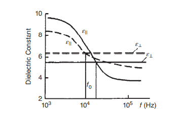
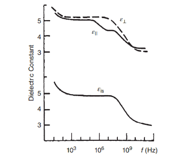
The two principal refractive indices $n_{\perp}$ and $n_{|}$of a uniaxial liquid crystal and the anisotropy $n_{|}-n_{\perp}$ have been the subject of intensive studies for their fundamental importance in the understanding of liquid crystal physics and for their vital roles in applied electro-optic devices. Since the dielectric constants $\left(\varepsilon_{\perp}\right.$ and $\left.\varepsilon_{||}\right)$enter directly and linearly into the constitutive equations (Eqs. (3.30a)-(3.30c)), it is theoretically more convenient to discuss the fundamentals of these temperature dependences in terms of the dielectric constants.

From Eq. (3.34) for the local field $\vec{E}^{\mathrm{loc}}$ and Eq. (3.31) for the induced dipole moments, we can express the polarization $\vec{p} \equiv N \vec{d}$ by
$$
\vec{P}=N \overrightarrow{\bar{\alpha}}:(\overrightarrow{\overrightarrow{\bar{K}}}: \vec{E})
$$
where $\overrightarrow{\bar{\alpha}}$ is the polarizability tensor of the molecule, $N$ is the number of molecules per unit volume, and the parentheses denote averaging over the orientations of all molecules.
The dielectric constant $\overrightarrow{\bar{\varepsilon}}$ (in units of $\varepsilon_0$ ) is therefore given by
$$
\overrightarrow{\vec{\varepsilon}}=1+\frac{N}{\varepsilon_0} \overrightarrow{\vec{\alpha}}: \overrightarrow{\vec{K}}
$$
and
$$
\begin{aligned}
\Delta \varepsilon &=\varepsilon_{|}-\varepsilon_{\perp} \
&=\frac{N}{\varepsilon_0}\left(\langle\overrightarrow{\vec{\alpha}}: \overrightarrow{\vec{K}}\rangle_{|}-\langle\overrightarrow{\vec{\alpha}}: \overrightarrow{\bar{K}}\rangle_{\perp}\right) .
\end{aligned}
$$
From these considerations and from observations by deJeu and Bordewijk [13] that
$$
\Delta \varepsilon \propto \rho S
$$

物理代写|光学代写Optics代考|Hydrodynamics of Ordinary Isotropic Fluids

Consider an elementary volume $d V=d x d y d z$ of a fluid moving in space as shown in Figure 3.9. The following parameters are needed to describe its dynamics:
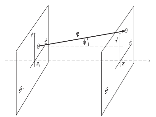
position vector: $\vec{r}$.
velucity: $\vec{v}(\vec{r}, t)$,
density: $\rho(\vec{r}, t)$,
pressure: $p(\vec{r}, t)$, and
forces in general: $\vec{f}(\vec{r}, t)$.
In later chapters where we study laser-induced acoustic (sound, density) waves in liquid crystals, or generally, when one deals with acoustic waves, it is necessary to assume that the density $\rho(\vec{r}, t)$ is a spatially and temporally varying function. In this chapter, however, we “decouple” such density wave excitation from all the processes under consideration and basically limit our attention to the flow and orientational effects of an incompressible fluid. In that case, we have
$$
\rho(\vec{r}, t)=\text { constant }
$$
For all liquids, in fact for all gas particles or charges in motion, the equation of continuity also holds
$$
\nabla \cdot(\rho \vec{v})=-\frac{\partial \rho}{\partial t} .
$$
This equation states that the total variation of $\rho \vec{v}$ over the surface of an enclosing volume is equal to the rate of decrease of the density. Since $\partial \rho / \partial t=0$, we thus have, from Eq. (3.51),
$$
\nabla \cdot \vec{v}=0
$$
The equation of motion describing the acceleration $d \vec{v} / d t$ of the fluid elements is simply Newton’s law:
$$
\rho \frac{d \vec{v}}{d t}=\vec{f}
$$

光学代考

物理代写|光学代写Optics代考|Equilibrium Temperature

两个主要折射率 $n_{\perp}$ 和 $n_{\mid}$单轴液晶和各向异性 $n_{\mid}-n_{\perp}$ 由于它们在理解液晶物理学方面的根本重要性以及它们在应 用电光器件中的重要作用，它们一直是深入研究的主题。由于介电常数 $\left(\varepsilon_{\perp}\right.$ 和 $\left.\varepsilon_{|}\right)$直接和线性地进入本构方程 (方 程 (3.30a) – (3.30c) )，理论上更方便根据介电常数讨论这些温度依赖性的基本原理。
从方程式。(3.34) 用于同部字段 $\vec{E}^{\text {loc }}$ 和等式。(3.31) 对于诱导偶极矩，我们可以表示极化 $\vec{p} \equiv N \vec{d}$ 经过
$$
\vec{P}=N \overrightarrow{\bar{\alpha}}:(\overrightarrow{\overrightarrow{\vec{K}}}: \vec{E})
$$
在哪里 $\overrightarrow{\vec{\alpha}}$ 是分子的极化张量， $N$ 是每单位体积的分子数，括号表示所有分子方向的平均值。
介电常数 $\vec{\varepsilon}$ (以 $\varepsilon_0$ ) 因此由下式给出
$$
\vec{\varepsilon}=1+\frac{N}{\varepsilon_0} \vec{\alpha}: \overrightarrow{\vec{K}}
$$
和
$$
\Delta \varepsilon=\varepsilon_{\mid}-\varepsilon_{\perp} \quad=\frac{N}{\varepsilon_0}\left(\langle\overrightarrow{\vec{\alpha}}: \overrightarrow{\vec{K}}\rangle_{\mid}-\langle\overrightarrow{\vec{\alpha}}: \overrightarrow{\bar{K}}\rangle_{\perp}\right)
$$
根据这些考虑以及 dejeu 和 Bordewijk [13] 的观察，
$\Delta \varepsilon \propto \rho S$

物理代写|光学代写Optics代考|Hydrodynamics of Ordinary Isotropic Fluids

考虑一个基本体积 $d V=d x d y d z$ 如图 $3.9$ 所示，流体在空间中移动。需要以下参数来描述其动力学:
位置向量: $\vec{r}$.
速度： $\vec{v}(\vec{r}, t)$ ，
密度: $\rho(\vec{r}, t)$ ，
压力： $p(\vec{r}, t)$ ，以及
一般的力： $\vec{f}(\vec{r}, t)$.
在后面我们研究液晶中激光诱导的声（声、密度）波的章节中，或者一般来说，当我们处理声波时，有必要假设 密度 $\rho(\vec{r}, t)$ 是一个空间和时间变化的函数。然而，在本章中，我们将这种密度波激发与所考虑的所有过程“分 离”，基本上将我们的注意力限制在不可压缩流体的流动和定向效应上。在这种情况下，我们有
$$
\rho(\vec{r}, t)=\text { constant }
$$
对于所有俻体，实际上对于所有运动中的气体粒子或电荷，连续性方程也成立
$$
\nabla \cdot(\rho \vec{v})=-\frac{\partial \rho}{\partial t} .
$$
这个方程表明，总变化 $\rho \vec{v}$ 在封闭体积的表面上等于密度的下降率。自从 $\partial \rho / \partial t=0$ ，因此我们有，从等式。 (3.51),
$$
\nabla \cdot \vec{v}=0
$$
描述加速度的运动方程 $d \vec{v} / d t$ 流体元素的定义就是牛顿定律:
$$
\rho \frac{d \vec{v}}{d t}=\vec{f}
$$

统计代写请认准statistics-lab™. statistics-lab™为您的留学生涯保驾护航。

金融工程代写

金融工程是使用数学技术来解决金融问题。金融工程使用计算机科学、统计学、经济学和应用数学领域的工具和知识来解决当前的金融问题，以及设计新的和创新的金融产品。

非参数统计代写

非参数统计指的是一种统计方法，其中不假设数据来自于由少数参数决定的规定模型；这种模型的例子包括正态分布模型和线性回归模型。

广义线性模型代考

广义线性模型（GLM）归属统计学领域，是一种应用灵活的线性回归模型。该模型允许因变量的偏差分布有除了正态分布之外的其它分布。

术语 广义线性模型（GLM）通常是指给定连续和/或分类预测因素的连续响应变量的常规线性回归模型。它包括多元线性回归，以及方差分析和方差分析（仅含固定效应）。

有限元方法代写

有限元方法（FEM）是一种流行的方法，用于数值解决工程和数学建模中出现的微分方程。典型的问题领域包括结构分析、传热、流体流动、质量运输和电磁势等传统领域。

有限元是一种通用的数值方法，用于解决两个或三个空间变量的偏微分方程（即一些边界值问题）。为了解决一个问题，有限元将一个大系统细分为更小、更简单的部分，称为有限元。这是通过在空间维度上的特定空间离散化来实现的，它是通过构建对象的网格来实现的：用于求解的数值域，它有有限数量的点。边界值问题的有限元方法表述最终导致一个代数方程组。该方法在域上对未知函数进行逼近。[1] 然后将模拟这些有限元的简单方程组合成一个更大的方程系统，以模拟整个问题。然后，有限元通过变化微积分使相关的误差函数最小化来逼近一个解决方案。

tatistics-lab作为专业的留学生服务机构，多年来已为美国、英国、加拿大、澳洲等留学热门地的学生提供专业的学术服务，包括但不限于Essay代写，Assignment代写，Dissertation代写，Report代写，小组作业代写，Proposal代写，Paper代写，Presentation代写，计算机作业代写，论文修改和润色，网课代做，exam代考等等。写作范围涵盖高中，本科，研究生等海外留学全阶段，辐射金融，经济学，会计学，审计学，管理学等全球99%专业科目。写作团队既有专业英语母语作者，也有海外名校硕博留学生，每位写作老师都拥有过硬的语言能力，专业的学科背景和学术写作经验。我们承诺100%原创，100%专业，100%准时，100%满意。

随机分析代写

随机微积分是数学的一个分支，对随机过程进行操作。它允许为随机过程的积分定义一个关于随机过程的一致的积分理论。这个领域是由日本数学家伊藤清在第二次世界大战期间创建并开始的。

时间序列分析代写

随机过程，是依赖于参数的一组随机变量的全体，参数通常是时间。 随机变量是随机现象的数量表现，其时间序列是一组按照时间发生先后顺序进行排列的数据点序列。通常一组时间序列的时间间隔为一恒定值（如1秒，5分钟，12小时，7天，1年），因此时间序列可以作为离散时间数据进行分析处理。研究时间序列数据的意义在于现实中，往往需要研究某个事物其随时间发展变化的规律。这就需要通过研究该事物过去发展的历史记录，以得到其自身发展的规律。

回归分析代写

多元回归分析渐进（Multiple Regression Analysis Asymptotics）属于计量经济学领域，主要是一种数学上的统计分析方法，可以分析复杂情况下各影响因素的数学关系，在自然科学、社会和经济学等多个领域内应用广泛。

MATLAB代写

MATLAB 是一种用于技术计算的高性能语言。它将计算、可视化和编程集成在一个易于使用的环境中，其中问题和解决方案以熟悉的数学符号表示。典型用途包括：数学和计算算法开发建模、仿真和原型制作数据分析、探索和可视化科学和工程图形应用程序开发，包括图形用户界面构建MATLAB 是一个交互式系统，其基本数据元素是一个不需要维度的数组。这使您可以解决许多技术计算问题，尤其是那些具有矩阵和向量公式的问题，而只需用 C 或 Fortran 等标量非交互式语言编写程序所需的时间的一小部分。MATLAB 名称代表矩阵实验室。MATLAB 最初的编写目的是提供对由 LINPACK 和 EISPACK 项目开发的矩阵软件的轻松访问，这两个项目共同代表了矩阵计算软件的最新技术。MATLAB 经过多年的发展，得到了许多用户的投入。在大学环境中，它是数学、工程和科学入门和高级课程的标准教学工具。在工业领域，MATLAB 是高效研究、开发和分析的首选工具。MATLAB 具有一系列称为工具箱的特定于应用程序的解决方案。对于大多数 MATLAB 用户来说非常重要，工具箱允许您学习和应用专业技术。工具箱是 MATLAB 函数（M 文件）的综合集合，可扩展 MATLAB 环境以解决特定类别的问题。可用工具箱的领域包括信号处理、控制系统、神经网络、模糊逻辑、小波、仿真等。

如果你也在 怎样代写光学Optics这个学科遇到相关的难题，请随时右上角联系我们的24/7代写客服。

光学是研究光的行为和属性的物理学分支，包括它与物质的相互作用以及使用或探测它的仪器的构造。光学通常描述可见光、紫外光和红外光的行为。

statistics-lab™ 为您的留学生涯保驾护航 在代写光学Optics方面已经树立了自己的口碑, 保证靠谱, 高质且原创的统计Statistics代写服务。我们的专家在代写光学Optics代写方面经验极为丰富，各种代写光学Optics相关的作业也就用不着说。

我们提供的光学Optics及其相关学科的代写，服务范围广, 其中包括但不限于:

• Statistical Inference 统计推断
• Statistical Computing 统计计算
• Advanced Probability Theory 高等概率论
• Advanced Mathematical Statistics 高等数理统计学
• (Generalized) Linear Models 广义线性模型
• Statistical Machine Learning 统计机器学习
• Longitudinal Data Analysis 纵向数据分析
• Foundations of Data Science 数据科学基础

物理代写|光学代写Optics代考|DIELECTRIC CONSTANTS AND REFRACTIVE INDICES

Dielectric constants and refractive indices, as well as electrical conductivities of liquid crystals, are physical parameters that characterize the electronic responses of liquid crystals to externally applied fields (electric, magnetic, or optical). Because of the molecular and energy level structures of nematic molecules, these responses are highly dependent on the direction and the frequencies of the field. Accordingly, we shall classify our studies of dielectric permittivity and other electro-optical parameters into two distinctive frequency regimes: (1) dc and low frequency and (2) optical frequency. Where the transition from the regime (1) to (2) occurs, of course, is governed by the dielectric relaxation processes and the dynamical time constant; typically, the Debye relaxation frequencies in nematics are on the order of $10^{10} \mathrm{~Hz}$.

Most nematics (e.g. E7, pentyl cyanobiphenyl [5CB], etc.) are said to possess positive (dielectric) anisotropy $\left(\varepsilon_{||}>\varepsilon_{\perp}\right)$. On the other hand, some nematics, such as MBBA, possess negative anisotropy (i.e. $\varepsilon_{|}<\varepsilon_{\perp}$ ). The controlling factors are the molecular constituents and structures.

In general, $\varepsilon_{|}$and $\varepsilon_{\perp}$ have different dispersion regions, as shown in Figure $3.4$ for 4-methoxy-4′-n-butylazoxy-benzene [7], which possess negative dielectric anisotropy $(\Delta \varepsilon<0)$. Also plotted in Figure $3.4$ is the dispersion of $\varepsilon_{\text {iso }}$, the dielectric constant for the isotropic case. Notice that for frequencies of $10^9 \mathrm{~Hz}$ or less, $\varepsilon_{\perp}>\varepsilon_{|}$. At higher frequencies and in the optical regime, $\varepsilon_{| 1}>\varepsilon_{\perp}$ (i.e. the dielectric anisotropy changes sign).

For some nematic liquid crystals, this changeover in the sign of $\Delta \varepsilon=\varepsilon_{|}-\varepsilon_{\perp}$ occurs at a much lower frequency (cf. Figure $3.5$ for phenylbenzoates [8]). This changeover frequency $f_{\mathrm{co}}$ is lower because of the long three-ringed molecular structure, which is highly resistant to the rotation of molecules around the short axes.

物理代写|光学代写Optics代考|Free Energy and Torques by Electric and Magnetic Fields

In this section, we consider the interactions of nematic liquid crystals with applied fields (electric or magnetic); we will limit our discussion to only dielectric and diamagnetic interactions.

For a generally applied (dc, low frequency, or optical) electric field $\vec{E}$, the displacement $\vec{D}$ may be written in the form
$$
\vec{D}=\varepsilon_{\perp} \vec{E}+\left(\varepsilon_{|}-\varepsilon_{\perp}\right)(n \cdot \vec{E}) n
$$

The electric interaction energy density is therefore
$$
\mu_E=-\int_0^E \vec{D} \cdot d \vec{E}=-\frac{1}{2} \varepsilon_{\perp}(\vec{E} \cdot \vec{E})-\frac{\Delta \varepsilon}{2}(n \cdot \vec{E})^2 .
$$
Note that the first term on the right-hand side of Eq. (3.24) is independent of the orientation of the director axis. It can therefore be neglected in the director axis deformation energy. Accordingly, the free-energy density term associated with the application of an electric field is given by
$$
F_E=-\frac{\Delta \varepsilon}{2}(n \cdot \vec{E})^2
$$
in SI units (in cgs units, $F_E=-(\Delta \varepsilon / 8 \pi)(\hat{n} \cdot \vec{E})^2$ ). The molecular torque produced by the electric field is given by
$$
\vec{\Gamma}E=\vec{D} \times \vec{E}=\Delta \varepsilon(n \cdot \vec{E})(n \times \vec{E}) . $$ Similar considerations for the magnetic field yield a magnetic energy density term $U_m$ given by $$ U_m=-\int_0^M \vec{B} \cdot d \vec{M}=\frac{1}{2 \mu_0} \chi{\perp}^m B^2-\frac{1}{2 \mu_0} \Delta \chi^m(n \cdot \vec{B})^2,
$$
a magnetic free-energy density (associated with director axis reorientation) $F_m$ given by
$$
F_m=\frac{1}{2 \mu_0} \Delta \chi^m(n \cdot \vec{B})^2,
$$
and a magnetic torque density
$$
\begin{aligned}
\vec{\Gamma}_m &=\vec{M} \times \vec{H} \
&=\Delta \chi^m(n \cdot \vec{H})(n \cdot \vec{H}) .
\end{aligned}
$$

光学代考

物理代写|光学代写Optics代考|DIELECTRIC CONSTANTS AND REFRACTIVE INDICES

介电常数和折射率以及液晶的电导率是表征液晶对外部施加场 (电场、磁场或光学) 的电子响应的物理参数。由 于向列分子的分子和能级结构，这些响应高度依赖于场的方向和频率。因此，我们将对介电常数和其他电光参数 的研究分为两个不同的频率范围：（1）直流和低频以及 (2) 光学频率。当然，从状态 (1) 到 (2) 的转变是由 介电弛豫过程和动态时间常数控制的；通常，向列相中的德拜驰豫频率约为 $10^{10} \mathrm{~Hz}$.
大多数向列体（例如 $\mathrm{E}$ 、戊基氛基联苯 [5CB] 等) 据说具有正（介电) 各向异性 $\left(\varepsilon_{|}>\varepsilon_{\perp}\right.$ ). 另一方面，一些向 列相，如 MBBA，具有负各向异性 $\left(\right.$ 即 $\left.\varepsilon_{\mid}<\varepsilon_{\perp}\right)$ 。控制因素是分子成分和结构。 一般来说， $\varepsilon_{\mid}$和 $\varepsilon_{\perp}$ 有不同的分散区域，如图3.4对于具有负介电各向异性的 4-methoxy-4′-n-butylazoxy-benzo $\varepsilon_{\perp}>\varepsilon_{\mid}$. 在较高频率和光学状态下， $\varepsilon_{\mid 1}>\varepsilon_{\perp}$ (即介电各向异性改变符号) 。
对于一些向列液晶，这种符号的转换 $\Delta \varepsilon=\varepsilon_{\mid}-\varepsilon_{\perp}$ 以低得多的频率发生 (参见图 $3.5$ 苯甲酸苯酯 [8])。这个转换

物理代写|光学代写Optics代考|Free Energy and Torques by Electric and Magnetic Fields

在本节中，我们考虑向列液晶与外加场（电场或磁场）的相互作用；我们将讨论仅限于介电和抗磁相互作用。
对于一般应用的 (直流、低频或光学) 电场 $\vec{E}$, 位移 $\vec{D}$ 可以写成形式
$$
\vec{D}=\varepsilon_{\perp} \vec{E}+\left(\varepsilon_{\mid}-\varepsilon_{\perp}\right)(n \cdot \vec{E}) n
$$
因此，电相互作用能量密度为
$$
\mu_E=-\int_0^E \vec{D} \cdot d \vec{E}=-\frac{1}{2} \varepsilon_{\perp}(\vec{E} \cdot \vec{E})-\frac{\Delta \varepsilon}{2}(n \cdot \vec{E})^2 .
$$
请注意，等式右侧的第一项。(3.24) 与导向轴的方向无关。因此在导向轴变形能量中可以忽略不计。因此，与施加 电场相关的自由能密度项由下式给出
$$
F_E=-\frac{\Delta \varepsilon}{2}(n \cdot \vec{E})^2
$$
以 SI 单位 (以 $\operatorname{cgs}$ 为单位， $F_E=-(\Delta \varepsilon / 8 \pi)(\hat{n} \cdot \vec{E})^2$ )。由电场产生的分子扭矩由下式给出
$$
\vec{\Gamma} E=\vec{D} \times \vec{E}=\Delta \varepsilon(n \cdot \vec{E})(n \times \vec{E}) .
$$
对磁场的类似考虑产生了磁能密度项 $U_m$ 由
$$
U_m=-\int_0^M \vec{B} \cdot d \vec{M}=\frac{1}{2 \mu_0} \chi \perp^m B^2-\frac{1}{2 \mu_0} \Delta \chi^m(n \cdot \vec{B})^2,
$$
磁自由能密度 (与导向轴重新定向相关) $F_m$ 由
$$
F_m=\frac{1}{2 \mu_0} \Delta \chi^m(n \cdot \vec{B})^2,
$$
和磁转矩密度
$$
\vec{\Gamma}_m=\vec{M} \times \vec{H} \quad=\Delta \chi^m(n \cdot \vec{H})(n \cdot \vec{H})
$$

统计代写请认准statistics-lab™. statistics-lab™为您的留学生涯保驾护航。

金融工程代写

金融工程是使用数学技术来解决金融问题。金融工程使用计算机科学、统计学、经济学和应用数学领域的工具和知识来解决当前的金融问题，以及设计新的和创新的金融产品。

非参数统计代写

非参数统计指的是一种统计方法，其中不假设数据来自于由少数参数决定的规定模型；这种模型的例子包括正态分布模型和线性回归模型。

广义线性模型代考

广义线性模型（GLM）归属统计学领域，是一种应用灵活的线性回归模型。该模型允许因变量的偏差分布有除了正态分布之外的其它分布。

术语 广义线性模型（GLM）通常是指给定连续和/或分类预测因素的连续响应变量的常规线性回归模型。它包括多元线性回归，以及方差分析和方差分析（仅含固定效应）。

有限元方法代写

有限元方法（FEM）是一种流行的方法，用于数值解决工程和数学建模中出现的微分方程。典型的问题领域包括结构分析、传热、流体流动、质量运输和电磁势等传统领域。

有限元是一种通用的数值方法，用于解决两个或三个空间变量的偏微分方程（即一些边界值问题）。为了解决一个问题，有限元将一个大系统细分为更小、更简单的部分，称为有限元。这是通过在空间维度上的特定空间离散化来实现的，它是通过构建对象的网格来实现的：用于求解的数值域，它有有限数量的点。边界值问题的有限元方法表述最终导致一个代数方程组。该方法在域上对未知函数进行逼近。[1] 然后将模拟这些有限元的简单方程组合成一个更大的方程系统，以模拟整个问题。然后，有限元通过变化微积分使相关的误差函数最小化来逼近一个解决方案。

tatistics-lab作为专业的留学生服务机构，多年来已为美国、英国、加拿大、澳洲等留学热门地的学生提供专业的学术服务，包括但不限于Essay代写，Assignment代写，Dissertation代写，Report代写，小组作业代写，Proposal代写，Paper代写，Presentation代写，计算机作业代写，论文修改和润色，网课代做，exam代考等等。写作范围涵盖高中，本科，研究生等海外留学全阶段，辐射金融，经济学，会计学，审计学，管理学等全球99%专业科目。写作团队既有专业英语母语作者，也有海外名校硕博留学生，每位写作老师都拥有过硬的语言能力，专业的学科背景和学术写作经验。我们承诺100%原创，100%专业，100%准时，100%满意。

随机分析代写

随机微积分是数学的一个分支，对随机过程进行操作。它允许为随机过程的积分定义一个关于随机过程的一致的积分理论。这个领域是由日本数学家伊藤清在第二次世界大战期间创建并开始的。

时间序列分析代写

随机过程，是依赖于参数的一组随机变量的全体，参数通常是时间。 随机变量是随机现象的数量表现，其时间序列是一组按照时间发生先后顺序进行排列的数据点序列。通常一组时间序列的时间间隔为一恒定值（如1秒，5分钟，12小时，7天，1年），因此时间序列可以作为离散时间数据进行分析处理。研究时间序列数据的意义在于现实中，往往需要研究某个事物其随时间发展变化的规律。这就需要通过研究该事物过去发展的历史记录，以得到其自身发展的规律。

回归分析代写

多元回归分析渐进（Multiple Regression Analysis Asymptotics）属于计量经济学领域，主要是一种数学上的统计分析方法，可以分析复杂情况下各影响因素的数学关系，在自然科学、社会和经济学等多个领域内应用广泛。

MATLAB代写

MATLAB 是一种用于技术计算的高性能语言。它将计算、可视化和编程集成在一个易于使用的环境中，其中问题和解决方案以熟悉的数学符号表示。典型用途包括：数学和计算算法开发建模、仿真和原型制作数据分析、探索和可视化科学和工程图形应用程序开发，包括图形用户界面构建MATLAB 是一个交互式系统，其基本数据元素是一个不需要维度的数组。这使您可以解决许多技术计算问题，尤其是那些具有矩阵和向量公式的问题，而只需用 C 或 Fortran 等标量非交互式语言编写程序所需的时间的一小部分。MATLAB 名称代表矩阵实验室。MATLAB 最初的编写目的是提供对由 LINPACK 和 EISPACK 项目开发的矩阵软件的轻松访问，这两个项目共同代表了矩阵计算软件的最新技术。MATLAB 经过多年的发展，得到了许多用户的投入。在大学环境中，它是数学、工程和科学入门和高级课程的标准教学工具。在工业领域，MATLAB 是高效研究、开发和分析的首选工具。MATLAB 具有一系列称为工具箱的特定于应用程序的解决方案。对于大多数 MATLAB 用户来说非常重要，工具箱允许您学习和应用专业技术。工具箱是 MATLAB 函数（M 文件）的综合集合，可扩展 MATLAB 环境以解决特定类别的问题。可用工具箱的领域包括信号处理、控制系统、神经网络、模糊逻辑、小波、仿真等。

如果你也在 怎样代写光学Optics这个学科遇到相关的难题，请随时右上角联系我们的24/7代写客服。

光学是研究光的行为和属性的物理学分支，包括它与物质的相互作用以及使用或探测它的仪器的构造。光学通常描述可见光、紫外光和红外光的行为。

statistics-lab™ 为您的留学生涯保驾护航 在代写光学Optics方面已经树立了自己的口碑, 保证靠谱, 高质且原创的统计Statistics代写服务。我们的专家在代写光学Optics代写方面经验极为丰富，各种代写光学Optics相关的作业也就用不着说。

我们提供的光学Optics及其相关学科的代写，服务范围广, 其中包括但不限于:

• Statistical Inference 统计推断
• Statistical Computing 统计计算
• Advanced Probability Theory 高等概率论
• Advanced Mathematical Statistics 高等数理统计学
• (Generalized) Linear Models 广义线性模型
• Statistical Machine Learning 统计机器学习
• Longitudinal Data Analysis 纵向数据分析
• Foundations of Data Science 数据科学基础

物理代写|光学代写Optics代考|When Must You Wear Laser Safety Glasses

The class of a laser must be printed on the laser housing. It’s usually shown somewhere near the aperture. Never use a laser whose class you do not know. If there is no label telling you the class and the wavelength, don’t use the laser! Also, never use a laser that has been tampered with because this can affect the output beam in unexpected ways. (Some lasers, such as green laser pointers, are actually frequency-doubled infrared lasers. The infrared component is typically prevented from leaving the laser by a filter. If that filter is broken or removed, you could receive a very hazardous eye exposure to an infrared beam without realizing it.) If the warning label on the laser says words like “danger” or “avoid exposure to beam” take it seriously!

Laser glasses should be obtained from a reputable supplier and should conform to national certification requirements. The ability of laser glasses to block radiation is described by the optical density (OD) rating for the wavelength of the laser in use. Higher OD, means more light attenuation. Note that an OD rating that is sufficiently high to be safe at one wavelength does not imply that the glasses are safe for any other laser wavelength. In general, different laser wavelengths require different safety glasses. The OD rating is a logarithmic scale that specifies the transmission of the glasses at the rated wavelength.
$$
\mathrm{OD}=\log _{10}\left(\frac{1}{T}\right)
$$
where $T$ is the transmittance of the glasses. The transmittance of the glasses is the fraction of incident power that is transmitted through the glasses. For example, if a set of laser glasses has an OD of 5 at $1,064 \mathrm{~nm}$, they will transmit 1/100,000th of the incident power at this wavelength.

物理代写|光学代写Optics代考|Good Safety Habits

If you inculcate good habits when working with lasers and associated optics, laser safety will become a natural way of working and not a burden. Many of these habits will also help with lab productivity in general. Here’s a list.
Remember the safety glasses
Keep safety glasses in a particular place. Make a habit of putting them on before turning on the laser! For keyed lasers, it can be a good reminder to store the key near the glasses.
Keep upright
Never put your eyes at the height of the beam. Other than wearing your safety glasses, this is the most important precaution you can take. Similarly, don’t bend down to get a dropped object or lean down over the optic chain in such a way as to bring your eyes near the height of the laser. When you are not upright, your safety glasses may not sit properly, potentially exposing you to a very hazardous situation.
No jewelry
Remove all reflective objects on your body or clothes before working with a laser. This includes watches, smartwatches, rings of all types, brooches, and so on. Hair should be tied back so as not to fall into the beam and so as not to contaminate the optics.
Horizontal beam path
If at all possible, keep the beam path at a single uniform height. Most importantly, avoid any beams that don’t travel horizontally. If you must change the beam height, use periscopes specifically designed for that purpose.
Close the shutter first
Always block the laser before adding or removing an optic. Usually, this is as simple as closing the laser shutter. Align a new optic as best you can without the beam. Then unblock the laser and adjust the alignment as required.

光学代考

物理代写|光学代写Optics代考|When Must You Wear Laser Safety Glasses

激光器的等级必须印在激光器外壳上。它通常显示在光圈附近的某个地方。切勿使用您不知道其类别的激光器。 如果没有标签告诉您类别和波长，请不要使用激光！此外，切勿使用被澃改过的激光器，因为这会以意想不到的 方式影响输出光束。（一些激光器，例如绿色激光指示器，实际上是倍频红外激光器。红外成分通常通过滤光片 阻止离开激光器。如果滤光片损坏或移除，您可能会受到非常危险的眼睛暴露于红外线光束而没有意识到。) 如 果激光上的警告标签上写㺺“危险”或“避免暴露于光束”之类的字眼，请认真对待!
激光眼镜应从信誉良好的供应商处获得，并应符合国家认证要求。激光玻璃阻挡辐射的能力由所用激光波长的光 密度 $(O D)$ 等级来描述。更高的OD，意味着更多的光哀减。请注意，OD 等级足够高以在一种波长下安全并不意 味着眼镜对任何其他激光波长都是安全的。一般来说，不同的激光波长需要不同的安全眼镜。OD 等级是一个对 数标度，用于指定玻璃在额定波长下的透射率。
$$
\mathrm{OD}=\log _{10}\left(\frac{1}{T}\right)
$$
在哪里 $T$ 是眼镜的透光率。玻璃的透射率是透过玻璃的入射功率的分数。例如，如果一副激光眼镜的 OD 为 5 ， $1,064 \mathrm{~nm}$ ，它们将在该波长传输 $1 / 100,000$ 的入射功率。

物理代写|光学代写Optics代考|Good Safety Habits

如果您在使用激光和相关光学器件时养成良好的习惯，激光安全将成为一种自然的工作方式，而不是一种负担。这些习惯中的许多也将有助于提高实验室的生产力。这是一个清单。
记住安全眼镜
将安全眼镜放在特定的地方。养成在打开激光之前戴上它们的习惯！对于键控激光器，将钥匙存放在眼镜附近可能是一个很好的提醒。
保持直立
切勿将眼睛放在光束的高度。除了戴上安全眼镜，这是您可以采取的最重要的预防措施。同样，不要弯腰捡起掉落的物体或俯身靠在光链上，以免眼睛靠近激光的高度。当您不直立时，您的安全眼镜可能无法正确放置，从而可能使您处于非常危险的境地。
无首饰
在使用激光之前，请去除身体或衣服上的所有反光物体。这包括手表、智能手表、所有类型的戒指、胸针等。头发应向后系好，以免落入光束中，以免污染光学器件。
水平光束路径
如果可能的话，将光束路径保持在一个统一的高度。最重要的是，避免任何不水平传播的光束。如果您必须更改光束高度，请使用专为此目的设计的潜望镜。
首先关闭快门
在添加或移除光学元件之前始终阻挡激光。通常，这就像关闭激光快门一样简单。在没有光束的情况下尽可能对准新的光学元件。然后打开激光并根据需要调整对准。

统计代写请认准statistics-lab™. statistics-lab™为您的留学生涯保驾护航。

金融工程代写

金融工程是使用数学技术来解决金融问题。金融工程使用计算机科学、统计学、经济学和应用数学领域的工具和知识来解决当前的金融问题，以及设计新的和创新的金融产品。

非参数统计代写

非参数统计指的是一种统计方法，其中不假设数据来自于由少数参数决定的规定模型；这种模型的例子包括正态分布模型和线性回归模型。

广义线性模型代考

广义线性模型（GLM）归属统计学领域，是一种应用灵活的线性回归模型。该模型允许因变量的偏差分布有除了正态分布之外的其它分布。

术语 广义线性模型（GLM）通常是指给定连续和/或分类预测因素的连续响应变量的常规线性回归模型。它包括多元线性回归，以及方差分析和方差分析（仅含固定效应）。

有限元方法代写

有限元方法（FEM）是一种流行的方法，用于数值解决工程和数学建模中出现的微分方程。典型的问题领域包括结构分析、传热、流体流动、质量运输和电磁势等传统领域。

有限元是一种通用的数值方法，用于解决两个或三个空间变量的偏微分方程（即一些边界值问题）。为了解决一个问题，有限元将一个大系统细分为更小、更简单的部分，称为有限元。这是通过在空间维度上的特定空间离散化来实现的，它是通过构建对象的网格来实现的：用于求解的数值域，它有有限数量的点。边界值问题的有限元方法表述最终导致一个代数方程组。该方法在域上对未知函数进行逼近。[1] 然后将模拟这些有限元的简单方程组合成一个更大的方程系统，以模拟整个问题。然后，有限元通过变化微积分使相关的误差函数最小化来逼近一个解决方案。

tatistics-lab作为专业的留学生服务机构，多年来已为美国、英国、加拿大、澳洲等留学热门地的学生提供专业的学术服务，包括但不限于Essay代写，Assignment代写，Dissertation代写，Report代写，小组作业代写，Proposal代写，Paper代写，Presentation代写，计算机作业代写，论文修改和润色，网课代做，exam代考等等。写作范围涵盖高中，本科，研究生等海外留学全阶段，辐射金融，经济学，会计学，审计学，管理学等全球99%专业科目。写作团队既有专业英语母语作者，也有海外名校硕博留学生，每位写作老师都拥有过硬的语言能力，专业的学科背景和学术写作经验。我们承诺100%原创，100%专业，100%准时，100%满意。

随机分析代写

随机微积分是数学的一个分支，对随机过程进行操作。它允许为随机过程的积分定义一个关于随机过程的一致的积分理论。这个领域是由日本数学家伊藤清在第二次世界大战期间创建并开始的。

时间序列分析代写

随机过程，是依赖于参数的一组随机变量的全体，参数通常是时间。 随机变量是随机现象的数量表现，其时间序列是一组按照时间发生先后顺序进行排列的数据点序列。通常一组时间序列的时间间隔为一恒定值（如1秒，5分钟，12小时，7天，1年），因此时间序列可以作为离散时间数据进行分析处理。研究时间序列数据的意义在于现实中，往往需要研究某个事物其随时间发展变化的规律。这就需要通过研究该事物过去发展的历史记录，以得到其自身发展的规律。

回归分析代写

多元回归分析渐进（Multiple Regression Analysis Asymptotics）属于计量经济学领域，主要是一种数学上的统计分析方法，可以分析复杂情况下各影响因素的数学关系，在自然科学、社会和经济学等多个领域内应用广泛。

MATLAB代写

MATLAB 是一种用于技术计算的高性能语言。它将计算、可视化和编程集成在一个易于使用的环境中，其中问题和解决方案以熟悉的数学符号表示。典型用途包括：数学和计算算法开发建模、仿真和原型制作数据分析、探索和可视化科学和工程图形应用程序开发，包括图形用户界面构建MATLAB 是一个交互式系统，其基本数据元素是一个不需要维度的数组。这使您可以解决许多技术计算问题，尤其是那些具有矩阵和向量公式的问题，而只需用 C 或 Fortran 等标量非交互式语言编写程序所需的时间的一小部分。MATLAB 名称代表矩阵实验室。MATLAB 最初的编写目的是提供对由 LINPACK 和 EISPACK 项目开发的矩阵软件的轻松访问，这两个项目共同代表了矩阵计算软件的最新技术。MATLAB 经过多年的发展，得到了许多用户的投入。在大学环境中，它是数学、工程和科学入门和高级课程的标准教学工具。在工业领域，MATLAB 是高效研究、开发和分析的首选工具。MATLAB 具有一系列称为工具箱的特定于应用程序的解决方案。对于大多数 MATLAB 用户来说非常重要，工具箱允许您学习和应用专业技术。工具箱是 MATLAB 函数（M 文件）的综合集合，可扩展 MATLAB 环境以解决特定类别的问题。可用工具箱的领域包括信号处理、控制系统、神经网络、模糊逻辑、小波、仿真等。

如果你也在 怎样代写光学Optics这个学科遇到相关的难题，请随时右上角联系我们的24/7代写客服。

光学是研究光的行为和属性的物理学分支，包括它与物质的相互作用以及使用或探测它的仪器的构造。光学通常描述可见光、紫外光和红外光的行为。

statistics-lab™ 为您的留学生涯保驾护航 在代写光学Optics方面已经树立了自己的口碑, 保证靠谱, 高质且原创的统计Statistics代写服务。我们的专家在代写光学Optics代写方面经验极为丰富，各种代写光学Optics相关的作业也就用不着说。

我们提供的光学Optics及其相关学科的代写，服务范围广, 其中包括但不限于:

• Statistical Inference 统计推断
• Statistical Computing 统计计算
• Advanced Probability Theory 高等概率论
• Advanced Mathematical Statistics 高等数理统计学
• (Generalized) Linear Models 广义线性模型
• Statistical Machine Learning 统计机器学习
• Longitudinal Data Analysis 纵向数据分析
• Foundations of Data Science 数据科学基础

物理代写|光学代写Optics代考|The Paraxial Approximation

We’re going to be most interested in the propagation of “beams” of light. ${ }^{2}$ Beams of light propagate mostly in one direction and we choose our axes so that the $z$-axis lies in the direction of propagation. The paraxial approximation is the assumption that all wavefront normals make small angles with the $z$-axis. It is appropriate for beams and any situation where light travels mostly in one direction. We consider the propagation between two planes perpendicular to the $z$-axis as shown in Figure 1.1: a source plane $\mathbf{S}{\mathbf{1}}$ at $z=z{1}$ and a “downstream” field plane $\mathbf{S}$ at some unspecified $z$. As before, we assume that in the source plane, the complex scalar field $\tilde{E}\left(x, y, z_{1}\right)$ is known.

The Helmholtz equation simplifies in the paraxial approximation. Since the light is propagating primarily in the z-direction, it’s useful to separate out the rapid phase accumulation in $z$ due to the wave nature of the light by writing
$$
\tilde{E}(x, y, z)=u(x, y, z) e^{-i k z} .
$$
The idea is that as long as the light is traveling largely in the $z$-direction, the $u(x, y, z)$ will vary very little over distances on the order of a wavelength. In other words, our wave can be treated as something close to a plane wave but with a complex amplitude $u(x, y, z)$ that varies slowly with position. $u(x, y, z)$ is sometimes known as the complex field amplitude or just the field amplitude. Substituting Eq. (1.22) into Eq. (1.9), we get
$$
\frac{\partial^{2} u}{\partial x^{2}}+\frac{\partial^{2} u}{\partial y^{2}}+\frac{\partial^{2} u}{\partial z^{2}}-2 i k \frac{\partial u}{\partial z}=0 .
$$
In the common case where the wave occupies only a small region in the source plane and the phasefronts are fairly flat – typical characteristics of what we might call “beams” then $u$ will vary more slowly in the z-direction than in any other direction, namely
$$
\begin{aligned}
&\left|\frac{\partial^{2} u}{\partial z^{2}}\right| \ll\left|\frac{\partial^{2} u}{\partial x^{2}}\right| \
&\left|\frac{\partial^{2} u}{\partial z^{2}}\right| \ll\left|\frac{\partial^{2} u}{\partial y^{2}}\right|
\end{aligned}
$$

物理代写|光学代写Optics代考|Coherence

Huygens’ principle also allows us to discuss one of the ways in which we classify the statistical properties of light. Light sources are often discussed in terms of their coherence, which comes in two types: temporal coherence and spatial coherence. In a temporally coherent emitter, all of the Huygens’ wavelets are emitting at the same frequency and the phase of each individual emitter remains fixed for a long time (e.g. many nanoseconds for a HeNe laser). This is known as the coherence time. Lasers have high temporal coherence compared to other sources of light. As a result, lasers tend to be very narrow-band emitters, emitting in only a very narrow band of wavelengths around some nominal wavelength. In lasers, the bandwidth of the output light is referred to as the “linewidth.” For example, HeNe lasers, which have fairly narrow linewidths, may emit wavelengths in the band $\lambda=$ $632.816 \pm 0.001 \mathrm{~nm}$. The coherence length of a HeNe is the distance traveled by the beam in the coherence time. For a HeNe, it’s typically a few tens of centimeters but can be tens of meters for carefully designed units.

High temporal coherence does not in itself require that all the Huygens’ emitters have the same phase, only that the phase of each individual emitter should vary slowly. Spatial coherence describes the phase relationship between the different Huygens’ emitters. In a source with high spatial coherence, all the emitters are in phase with one another, or nearly so. For example, Young’s double-slit experiment only yields the expected diffraction pattern when the spatial coherence of the incident light is sufficient that parts of the beam separated by the slit distance have similar phase. Sources with high spatial coherence can be focused to very small spot sizes and can be collimated so that they approximate plane waves. Note that high spatial coherence does not require high temporal coherence even though they usually occur together. As long as the phases of all the emitters stay the same, spatial coherence is preserved whether the overall phase changes are fast or slow, random or not. In Chapter 6, we discuss the properties of etendue and radiance, which are closely related to spatial coherence. Sources with high spatial coherence will have high radiance and low etendue. As a rule, both the temporal and spatial coherence of lasers are the highest of all light sources, which is the main reason they’re so useful.

光学代考

物理代写|光学代写Optics代考|The Paraxial Approximation

我们将对”光束”的传播最感兴趣。 ${ }^{2}$ 光束主要在一个方向上传播，我们选择我们的轴，以便 $z$-轴位于传播方向。近 轴近似是假设所有波前法线与 $z$-轴。它适用于光束和光主要沿一个方向传播的任何情况。我们考虑垂直于 $z$ 轴如图 $1.1$ 所示: 一个源平面 $\mathbf{S} 1$ 在 $z=z 1$ 和“下游”场平面 $\mathbf{S}$ 在一些末指定的 $z$. 和以前一样，我们假设在源平面中，复标 量场 $\tilde{E}\left(x, y, z_{1}\right)$ 是已知的。
亥姆霍兹方程简化了近轴近似。由于光主要在 $z$ 方向传播，因此将快速相位男积分离出来是有用的 $z$ 由于光的波动 性，通过书写
$$
\tilde{E}(x, y, z)=u(x, y, z) e^{-i k z}
$$
这个想法是，只要光主要在 $z$-方向， $u(x, y, z)$ 在波长数量级的距离上变化很小。换句话说，我们的波可以被视为 接近平面波但具有复振幅的东西 $u(x, y, z)$ 随位置缓慢变化。 $u(x, y, z)$ 有时称为复场幅度或仅称为场幅度。代入 方程式。(1.22) 进入等式。(1.9)，我们得到
$$
\frac{\partial^{2} u}{\partial x^{2}}+\frac{\partial^{2} u}{\partial y^{2}}+\frac{\partial^{2} u}{\partial z^{2}}-2 i k \frac{\partial u}{\partial z}=0 .
$$
在常见的情况下，波只占据源平面中的一个小区域并且相前相当平坦一一我们可以称之为“光束“的典型特征然后 $u$ 将在 z 方向上比在任何其他方向上变化得更慢，即
$$
\left|\frac{\partial^{2} u}{\partial z^{2}}\right| \ll\left|\frac{\partial^{2} u}{\partial x^{2}}\right| \quad\left|\frac{\partial^{2} u}{\partial z^{2}}\right| \ll\left|\frac{\partial^{2} u}{\partial y^{2}}\right|
$$

物理代写|光学代写Optics代考|Coherence

惠更斯原理还允许我们讨论对光的统计特性进行分类的一种方法。光源通常根据它们的相干性来讨论，它有两种类型：时间相干性和空间相干性。在时间相干发射器中，所有惠更斯小波都以相同的频率发射，并且每个发射器的相位在很长一段时间内保持固定（例如，对于氦氖激光器来说是许多纳秒）。这被称为相干时间。与其他光源相比，激光具有较高的时间相干性。因此，激光器往往是非常窄带的发射器，仅在某个标称波长附近的非常窄的波长带中发射。在激光器中，输出光的带宽称为“线宽”。例如，氦氖激光器，其线宽相当窄，l= 632.816±0.001 n米. HeNe 的相干长度是光束在相干时间内行进的距离。对于氦氖，它通常是几十厘米，但对于精心设计的单元来说可能是几十米。

高时间相干性本身并不要求所有惠更斯发射器具有相同的相位，只是每个单独的发射器的相位应该缓慢变化。空间相干性描述了不同惠更斯发射器之间的相位关系。在具有高空间相干性的源中，所有发射器彼此同相，或几乎同相。例如，当入射光的空间相干性足以使被狭缝距离分开的部分光束具有相似的相位时，Young 的双缝实验只会产生预期的衍射图案。具有高空间相干性的源可以聚焦到非常小的光斑尺寸，并且可以进行准直，使它们接近平面波。请注意，高空间相干性不需要高时间相干性，即使它们通常一起出现。只要所有发射器的相位保持相同，无论整体相位变化是快还是慢、随机与否，都可以保持空间相干性。在第 6 章中，我们讨论了与空间相干性密切相关的光展量和辐射度的性质。具有高空间相干性的光源将具有高辐射度和低光展度。通常，激光的时间相干性和空间相干性都是所有光源中最高的，这也是它们如此有用的主要原因。

统计代写请认准statistics-lab™. statistics-lab™为您的留学生涯保驾护航。

金融工程代写

金融工程是使用数学技术来解决金融问题。金融工程使用计算机科学、统计学、经济学和应用数学领域的工具和知识来解决当前的金融问题，以及设计新的和创新的金融产品。

非参数统计代写

非参数统计指的是一种统计方法，其中不假设数据来自于由少数参数决定的规定模型；这种模型的例子包括正态分布模型和线性回归模型。

广义线性模型代考

广义线性模型（GLM）归属统计学领域，是一种应用灵活的线性回归模型。该模型允许因变量的偏差分布有除了正态分布之外的其它分布。

术语 广义线性模型（GLM）通常是指给定连续和/或分类预测因素的连续响应变量的常规线性回归模型。它包括多元线性回归，以及方差分析和方差分析（仅含固定效应）。

有限元方法代写

有限元方法（FEM）是一种流行的方法，用于数值解决工程和数学建模中出现的微分方程。典型的问题领域包括结构分析、传热、流体流动、质量运输和电磁势等传统领域。

有限元是一种通用的数值方法，用于解决两个或三个空间变量的偏微分方程（即一些边界值问题）。为了解决一个问题，有限元将一个大系统细分为更小、更简单的部分，称为有限元。这是通过在空间维度上的特定空间离散化来实现的，它是通过构建对象的网格来实现的：用于求解的数值域，它有有限数量的点。边界值问题的有限元方法表述最终导致一个代数方程组。该方法在域上对未知函数进行逼近。[1] 然后将模拟这些有限元的简单方程组合成一个更大的方程系统，以模拟整个问题。然后，有限元通过变化微积分使相关的误差函数最小化来逼近一个解决方案。

tatistics-lab作为专业的留学生服务机构，多年来已为美国、英国、加拿大、澳洲等留学热门地的学生提供专业的学术服务，包括但不限于Essay代写，Assignment代写，Dissertation代写，Report代写，小组作业代写，Proposal代写，Paper代写，Presentation代写，计算机作业代写，论文修改和润色，网课代做，exam代考等等。写作范围涵盖高中，本科，研究生等海外留学全阶段，辐射金融，经济学，会计学，审计学，管理学等全球99%专业科目。写作团队既有专业英语母语作者，也有海外名校硕博留学生，每位写作老师都拥有过硬的语言能力，专业的学科背景和学术写作经验。我们承诺100%原创，100%专业，100%准时，100%满意。

随机分析代写

随机微积分是数学的一个分支，对随机过程进行操作。它允许为随机过程的积分定义一个关于随机过程的一致的积分理论。这个领域是由日本数学家伊藤清在第二次世界大战期间创建并开始的。

时间序列分析代写

随机过程，是依赖于参数的一组随机变量的全体，参数通常是时间。 随机变量是随机现象的数量表现，其时间序列是一组按照时间发生先后顺序进行排列的数据点序列。通常一组时间序列的时间间隔为一恒定值（如1秒，5分钟，12小时，7天，1年），因此时间序列可以作为离散时间数据进行分析处理。研究时间序列数据的意义在于现实中，往往需要研究某个事物其随时间发展变化的规律。这就需要通过研究该事物过去发展的历史记录，以得到其自身发展的规律。

回归分析代写

多元回归分析渐进（Multiple Regression Analysis Asymptotics）属于计量经济学领域，主要是一种数学上的统计分析方法，可以分析复杂情况下各影响因素的数学关系，在自然科学、社会和经济学等多个领域内应用广泛。

MATLAB代写

MATLAB 是一种用于技术计算的高性能语言。它将计算、可视化和编程集成在一个易于使用的环境中，其中问题和解决方案以熟悉的数学符号表示。典型用途包括：数学和计算算法开发建模、仿真和原型制作数据分析、探索和可视化科学和工程图形应用程序开发，包括图形用户界面构建MATLAB 是一个交互式系统，其基本数据元素是一个不需要维度的数组。这使您可以解决许多技术计算问题，尤其是那些具有矩阵和向量公式的问题，而只需用 C 或 Fortran 等标量非交互式语言编写程序所需的时间的一小部分。MATLAB 名称代表矩阵实验室。MATLAB 最初的编写目的是提供对由 LINPACK 和 EISPACK 项目开发的矩阵软件的轻松访问，这两个项目共同代表了矩阵计算软件的最新技术。MATLAB 经过多年的发展，得到了许多用户的投入。在大学环境中，它是数学、工程和科学入门和高级课程的标准教学工具。在工业领域，MATLAB 是高效研究、开发和分析的首选工具。MATLAB 具有一系列称为工具箱的特定于应用程序的解决方案。对于大多数 MATLAB 用户来说非常重要，工具箱允许您学习和应用专业技术。工具箱是 MATLAB 函数（M 文件）的综合集合，可扩展 MATLAB 环境以解决特定类别的问题。可用工具箱的领域包括信号处理、控制系统、神经网络、模糊逻辑、小波、仿真等。

如果你也在 怎样代写光学Optics这个学科遇到相关的难题，请随时右上角联系我们的24/7代写客服。

光学是研究光的行为和属性的物理学分支，包括它与物质的相互作用以及使用或探测它的仪器的构造。光学通常描述可见光、紫外光和红外光的行为。

statistics-lab™ 为您的留学生涯保驾护航 在代写光学Optics方面已经树立了自己的口碑, 保证靠谱, 高质且原创的统计Statistics代写服务。我们的专家在代写光学Optics代写方面经验极为丰富，各种代写光学Optics相关的作业也就用不着说。

我们提供的光学Optics及其相关学科的代写，服务范围广, 其中包括但不限于:

• Statistical Inference 统计推断
• Statistical Computing 统计计算
• Advanced Probability Theory 高等概率论
• Advanced Mathematical Statistics 高等数理统计学
• (Generalized) Linear Models 广义线性模型
• Statistical Machine Learning 统计机器学习
• Longitudinal Data Analysis 纵向数据分析
• Foundations of Data Science 数据科学基础

物理代写|光学代写Optics代考|Maxwell’s Equations

The field of optics describes the behavior of light as it propagates through space and materials. To understand the behavior of light, we start with the fundamental classical physics model describing it: Maxwell’s equations of electrodynamics. Maxwell’s equations show that the electric and magnetic fields can travel as waves. In a source-free region, Maxwell’s equations in linear media are $^{1}$
$$
\begin{aligned}
\vec{\nabla} \cdot \vec{E} &=0, \
\vec{\nabla} \cdot \vec{B} &=0, \
\vec{\nabla} \times \vec{E} &=-\frac{\partial \vec{B}}{\partial t}, \
\vec{\nabla} \times \vec{B} &=\mu \epsilon \frac{\partial \vec{E}}{\partial t},
\end{aligned}
$$
where $\vec{E}$ is the electric field, $\vec{B}$ is the magnetic field, $\mu$ is the permeability of the medium, and $\epsilon$ is the permittivity of the medium. If we take the curl of both sides of Eq. (1.3), apply the vector identity $\vec{\nabla} \times \vec{\nabla} \times \vec{E}=\vec{\nabla}(\vec{\nabla} \cdot \vec{E})-\nabla^{2} \vec{E}$ to the left-hand side and exchange the order of the time derivative and the curl on the right-hand side, we get
$$
\vec{\nabla}(\vec{\nabla} \cdot \vec{E})-\nabla^{2} \vec{E}=-\frac{\partial(\vec{\nabla} \times \vec{B})}{\partial t} .
$$
Then substitute from Eqs. (1.1) and (1.4) to get
$$
\nabla^{2} \vec{E}=\mu \epsilon \frac{\partial^{2} \vec{E}}{\partial t^{2}} .
$$
This is the wave equation in three dimensions where the wave speed is $v=1 / \sqrt{\mu \epsilon}$. Taking the curl of Eq. (1.4) and performing similar algebra shows that the magnetic field also satisfies the wave equation with the same wave speed. Thus Maxwell’s equations allow for electromagnetic waves. In vacuum, the speed is $v=1 / \sqrt{\mu_{0} \epsilon_{0}} \equiv c$, the speed of light in vacuum. Light is indeed an electromagnetic wave.

We now look for solutions to Eq. (1.6) and its magnetic field counterpart. We actually only need to solve for the electric field because the magnetic field can always be found from $\vec{B}=\frac{1}{c} \hat{k} \times \vec{E}$, where $\hat{k}$ is the direction of travel.

物理代写|光学代写Optics代考|Huygens’ Principle

In many cases of interest in optics, Eq. (1.9) is solved to a good approximation by Huygens’ integral. The field is assumed to be known on a “source plane” $S_{1}$ perpendicular to the $z$-axis and is only nonzero in some finite region of that plane. The values of the field on $S_{1}$ serve as a boundary condition for solving Eq. (1.9). The solution is given by Huygens’ integral for the complex scalar field at any desired point $x, y, z$.
$$
\tilde{E}(x, y, z)=\frac{i}{\lambda} \iint_{S_{1}} \tilde{E}\left(x^{\prime}, y^{\prime}, z^{\prime}\right) \cos \phi \frac{e^{-i k r}}{r} \mathrm{~d} S^{\prime} .
$$
The integration over the source plane $S_{1}$ is performed using the integration variables $x^{\prime}$, $y^{\prime}, z^{\prime}$. The vector $\vec{r}$ joins points in the source plane $S_{1}$ with the point $(x, y, z)$ at which we are calculating the field. The angle between $\vec{r}$ and the z-axis is $\phi$ (see Figure 1.1). The solution represented by Huygens’ integral is satisfying because it encapsulates an intuitive understanding of how light waves behave that was understood long before the formal mathematics was fully worked out.

The intuitive description of Eq. (1.10) is known as Huygens’ principle, due to Christiaan Huygens (1629-1695), a Dutch mathematician and scientist. Under Huygens’ principle, every point in the source is considered to be emitting light with spherical wavefronts propagating outward – the so-called Huygens’ wavelets. These wavefronts are represented by the factor $\cos \phi \frac{e^{–i t}}{r}$. They are emitted preferentially in the direction perpendicular to the source plane due to the presence of $\cos \phi$. The constant $\frac{i}{\lambda}$ out-front contributes $90^{\circ}$ of phase and the $\lambda$ in the denominator serves to keep the units the same on both sides of the equation. The complex scalar field in the source plane $E\left(x, y, z_{1}\right)$ sets the relative amplitudes and phases of these tiny spherical emitters. The field $\tilde{F}(x, y, z)$ is then simply the linear superposition of all the spherical wavefronts emitted from the source.

光学代考

物理代写|光学代写Optics代考|Maxwell’s Equations

光学领域描述了光在空间和材料中传播时的行为。为了理解光的行为，我们从描述它的基本经典物理模型开始:
麦克斯韦电动力学方程。麦克斯韦方程表明电场和磁场可以像波一样传播。在无源区域，线性介质中的麦克斯韦 方程组为 $^{1}$
$$
\vec{\nabla} \cdot \vec{E}=0, \vec{\nabla} \cdot \vec{B} \quad=0, \vec{\nabla} \times \vec{E}=-\frac{\partial \vec{B}}{\partial t}, \vec{\nabla} \times \vec{B} \quad=\mu \epsilon \frac{\partial \vec{E}}{\partial t},
$$
在哪里 $\vec{E}$ 是电场， $\vec{B}$ 是磁场， $\mu$ 是介质的渗透率，并且 $\epsilon$ 是介质的介电常数。如果我们取等式两边的卷曲。(1.3)、 应用向量恒等式 $\vec{\nabla} \times \vec{\nabla} \times \vec{E}=\vec{\nabla}(\vec{\nabla} \cdot \vec{E})-\nabla^{2} \vec{E}$ 到左边，交换时间导数的顺序和右边的curl，我们得到
$$
\vec{\nabla}(\vec{\nabla} \cdot \vec{E})-\nabla^{2} \vec{E}=-\frac{\partial(\vec{\nabla} \times \vec{B})}{\partial t}
$$
然后从方程式替换。(1.1)和 (1.4) 得到
$$
\nabla^{2} \vec{E}=\mu \epsilon \frac{\partial^{2} \vec{E}}{\partial t^{2}}
$$
这是波速为的三维波动方程 $v=1 / \sqrt{\mu \epsilon}$. 以方程的卷曲。(1.4) 并执行类似的代数表明，磁场也满足具有相同波速 的波动方程。因此麦克斯韦方程允许电磁波。在真空中，速度为 $v=1 / \sqrt{\mu_{0} \epsilon_{0}} \equiv c$ ，真空中的光速。光确实是 一种电磁波。
我们现在寻找方程的解决方案。(1.6) 及其磁场对应物。我们实际上只需要求解电场，因为磁场总是可以从 $\vec{B}=\frac{1}{c} \hat{k} \times \vec{E}$ ，在哪里 $\hat{k}$ 是行进的方向。

物理代写|光学代写Optics代考|Huygens’ Principle

在许多对光学感兴趣的情况下，方程式。(1.9) 通过惠更斯积分求解到一个很好的近似值。假定该场在“源平面”上 是已知的 $S_{1}$ 垂直于 $z$-轴，并且仅在该平面的某些有限区域中非零。字段的值 $S_{1}$ 作为求解方程的边界条件。(1.9)。 解由惠更斯积分在任何所需点处对复标量场给出 $x, y, z$.
$$
\tilde{E}(x, y, z)=\frac{i}{\lambda} \iint_{S_{1}} \tilde{E}\left(x^{\prime}, y^{\prime}, z^{\prime}\right) \cos \phi \frac{e^{-i k r}}{r} \mathrm{~d} S^{\prime} .
$$
源平面上的集成 $S_{1}$ 使用积分变量执行 $x^{\prime}, y^{\prime}, z^{\prime}$. 向量 $\vec{r}$ 连接源平面中的点 $S_{1}$ 有一点 $(x, y, z)$ 我们正在计算该字 段。之间的角度 $\vec{r}$ z轴是 $\phi$ (见图 1.1) 。惠更斯积分所代表的解决方案是令人满意的，因为它封装了对光波行为方 式的直观理解，这种理解早在正式数学完全解决之前就已被理解。
方程的直观描述。(1.10) 因荷兰数学家和科学家克里斯蒂安.惠更斯 (1629-1695) 而被称为惠更斯原理。根据惠更 斯原理，光源中的每个点都被认为是发射具有向外传播的球形波前的光一一即所谓的惠更斯小波。这些波前由因 子表示 $\cos \phi \frac{e^{-i t}}{r}$. 由于存在 $\cos \phi$. 常数 $\frac{i}{\lambda}$ 前线贡献 $90^{\circ}$ 相位和 $\lambda$ 分母中的单位用于保持等式两边的单位相同。源平 面中的复标量场 $E\left(x, y, z_{1}\right)$ 设置这些微小球形发射器的相对幅度和相位。场 $\tilde{F}(x, y, z)$ 然后是从源发射的所有球面波前的简单线性叠加。

统计代写请认准statistics-lab™. statistics-lab™为您的留学生涯保驾护航。

金融工程代写

金融工程是使用数学技术来解决金融问题。金融工程使用计算机科学、统计学、经济学和应用数学领域的工具和知识来解决当前的金融问题，以及设计新的和创新的金融产品。

非参数统计代写

非参数统计指的是一种统计方法，其中不假设数据来自于由少数参数决定的规定模型；这种模型的例子包括正态分布模型和线性回归模型。

广义线性模型代考

广义线性模型（GLM）归属统计学领域，是一种应用灵活的线性回归模型。该模型允许因变量的偏差分布有除了正态分布之外的其它分布。

术语 广义线性模型（GLM）通常是指给定连续和/或分类预测因素的连续响应变量的常规线性回归模型。它包括多元线性回归，以及方差分析和方差分析（仅含固定效应）。

有限元方法代写

有限元方法（FEM）是一种流行的方法，用于数值解决工程和数学建模中出现的微分方程。典型的问题领域包括结构分析、传热、流体流动、质量运输和电磁势等传统领域。

有限元是一种通用的数值方法，用于解决两个或三个空间变量的偏微分方程（即一些边界值问题）。为了解决一个问题，有限元将一个大系统细分为更小、更简单的部分，称为有限元。这是通过在空间维度上的特定空间离散化来实现的，它是通过构建对象的网格来实现的：用于求解的数值域，它有有限数量的点。边界值问题的有限元方法表述最终导致一个代数方程组。该方法在域上对未知函数进行逼近。[1] 然后将模拟这些有限元的简单方程组合成一个更大的方程系统，以模拟整个问题。然后，有限元通过变化微积分使相关的误差函数最小化来逼近一个解决方案。

tatistics-lab作为专业的留学生服务机构，多年来已为美国、英国、加拿大、澳洲等留学热门地的学生提供专业的学术服务，包括但不限于Essay代写，Assignment代写，Dissertation代写，Report代写，小组作业代写，Proposal代写，Paper代写，Presentation代写，计算机作业代写，论文修改和润色，网课代做，exam代考等等。写作范围涵盖高中，本科，研究生等海外留学全阶段，辐射金融，经济学，会计学，审计学，管理学等全球99%专业科目。写作团队既有专业英语母语作者，也有海外名校硕博留学生，每位写作老师都拥有过硬的语言能力，专业的学科背景和学术写作经验。我们承诺100%原创，100%专业，100%准时，100%满意。

随机分析代写

随机微积分是数学的一个分支，对随机过程进行操作。它允许为随机过程的积分定义一个关于随机过程的一致的积分理论。这个领域是由日本数学家伊藤清在第二次世界大战期间创建并开始的。

时间序列分析代写

随机过程，是依赖于参数的一组随机变量的全体，参数通常是时间。 随机变量是随机现象的数量表现，其时间序列是一组按照时间发生先后顺序进行排列的数据点序列。通常一组时间序列的时间间隔为一恒定值（如1秒，5分钟，12小时，7天，1年），因此时间序列可以作为离散时间数据进行分析处理。研究时间序列数据的意义在于现实中，往往需要研究某个事物其随时间发展变化的规律。这就需要通过研究该事物过去发展的历史记录，以得到其自身发展的规律。

回归分析代写

多元回归分析渐进（Multiple Regression Analysis Asymptotics）属于计量经济学领域，主要是一种数学上的统计分析方法，可以分析复杂情况下各影响因素的数学关系，在自然科学、社会和经济学等多个领域内应用广泛。

MATLAB代写

MATLAB 是一种用于技术计算的高性能语言。它将计算、可视化和编程集成在一个易于使用的环境中，其中问题和解决方案以熟悉的数学符号表示。典型用途包括：数学和计算算法开发建模、仿真和原型制作数据分析、探索和可视化科学和工程图形应用程序开发，包括图形用户界面构建MATLAB 是一个交互式系统，其基本数据元素是一个不需要维度的数组。这使您可以解决许多技术计算问题，尤其是那些具有矩阵和向量公式的问题，而只需用 C 或 Fortran 等标量非交互式语言编写程序所需的时间的一小部分。MATLAB 名称代表矩阵实验室。MATLAB 最初的编写目的是提供对由 LINPACK 和 EISPACK 项目开发的矩阵软件的轻松访问，这两个项目共同代表了矩阵计算软件的最新技术。MATLAB 经过多年的发展，得到了许多用户的投入。在大学环境中，它是数学、工程和科学入门和高级课程的标准教学工具。在工业领域，MATLAB 是高效研究、开发和分析的首选工具。MATLAB 具有一系列称为工具箱的特定于应用程序的解决方案。对于大多数 MATLAB 用户来说非常重要，工具箱允许您学习和应用专业技术。工具箱是 MATLAB 函数（M 文件）的综合集合，可扩展 MATLAB 环境以解决特定类别的问题。可用工具箱的领域包括信号处理、控制系统、神经网络、模糊逻辑、小波、仿真等。

如果你也在 怎样代写光学Optics这个学科遇到相关的难题，请随时右上角联系我们的24/7代写客服。

光学是研究光的行为和属性的物理学分支，包括它与物质的相互作用以及使用或探测它的仪器的构造。光学通常描述可见光、紫外光和红外光的行为。

statistics-lab™ 为您的留学生涯保驾护航 在代写光学Optics方面已经树立了自己的口碑, 保证靠谱, 高质且原创的统计Statistics代写服务。我们的专家在代写光学Optics代写方面经验极为丰富，各种代写光学Optics相关的作业也就用不着说。

我们提供的光学Optics及其相关学科的代写，服务范围广, 其中包括但不限于:

• Statistical Inference 统计推断
• Statistical Computing 统计计算
• Advanced Probability Theory 高等概率论
• Advanced Mathematical Statistics 高等数理统计学
• (Generalized) Linear Models 广义线性模型
• Statistical Machine Learning 统计机器学习
• Longitudinal Data Analysis 纵向数据分析
• Foundations of Data Science 数据科学基础

物理代写|光学代写Optics代考|Functionalized and Discotic Liquid Crystals

Through various chemical synthesis techniques as well as nanotechnologies, an entire class of novel or so-called functionalized liquid crystals have emerged [11-13]. Figure $1.14$ shows, for example, the shuttlecock-shaped liquid crystal formed by incorporating fullerene $\mathrm{C} 60$ to various crystals and liquid crystals reported by Sawamura et al. [11]. Others have investigated a special class of liquid crystals comprising disc-like molecules, discotic liquid crystals, that possess interesting and useful semiconducting properties suitable for optoelectronic applications [12, 13].

In general, temperature ranges for the various mesophases of single constituent liquid crystals are quite limited. Therefore, while many fundamental studies are still conducted on such liquid crystalline materials, industrial applications employ mostly mixturēs, composites, or specially doped liquid crystals with large operrating temperature range and tailor-made physical and optical properties.

There are many techniques for modifying the physical properties of a liquid crystal. At the most fundamental level, various chemical groups such as bonds or atoms can be introduced to modify the LC molecule. A good example is the cyanobiphenyl homologous series $n \mathrm{CB}(n=1,2,3 \ldots$ ). As $n$ is increased through synthesis, the viscosities, anisotropies, molecular sizes, and many other parameters are greatly modified. Some of these physical properties can also be modified by substitution. For example, the hydrogen in the 2,3 , and 4 positions of the phenyl ring may be substituted by some fluoro $(\mathrm{F})$ or chloro $(\mathrm{Cl})$ group [14].

Besides these molecular synthesis techniques, there are other ways to dramatically improve the performance characteristics of liquid crystals. In the following sections, we describe three well-developed methods, focusing our discussion on nematic liquid crystals as they exemplify the unique characteristics of liquid crystals widely used in optical and photonic applications.

物理代写|光学代写Optics代考|Dye-doped Liquid Crystals

An obvious effect of introducing dye molecule to liquid crystals is to increase the absorption of a particular liquid crystal at some specified wavelength region. In particular, dye molecules with absorption anisotropy, or those that undergo conformation changes such as trans-cis isomorphism or produce photo-charges, are often used for photonic applications [15-17]. For example, dichroic dye molecules that are more absorptive for optical field polarization parallel than perpendicular to its long axis are often used for the guest-host effect as their oblong shape makes them compatible for dispersing in the host nematic liquid crystals without disturbing the order. These dichroic molecules can then be oriented and reoriented by an external field applied to the host NLC to switch the transmission of the cell (cf. Figure 1.17); such dichroic dye-doped liquid crystals have been utilized to demonstrate optical diode action [15] in the transmission of polarized light.

If the dye molecules undergo some physical changes such as trans-cis isomorphism or produce space charges following photon absorption, they could give rise to nonlinear optical effects [16]; others [17] have shown that dye molecules deposited on the cell windows can be optically aligned as an effective means of surface alignment mechanism for I.C. cell fahrication. These and other effects due to the presence of dye molecules or other photosensitive agents in liquid crystals are discussed in more detail in Chapter 8 .

光学代考

物理代写|光学代写Optics代考|Functionalized and Discotic Liquid Crystals

通过各种化学合成技术以及纳米技术，出现了一整类新型或所谓的功能化液晶[11-13]。数字1.14例如，显示了通过结合富勒烯形成的羽毛球状液晶C60Sawamura 等人 报道的各种晶体和液晶。[11]。其他人研究了一类特殊的液晶，包括盘状分子，盘状液晶，它具有适合光电应用的有趣和有用的半导体特性 [12, 13]。

通常，单组分液晶的各种中间相的温度范围非常有限。因此，尽管仍在对此类液晶材料进行许多基础研究，但工业应用主要采用具有大工作温度范围和定制物理和光学特性的混合物、复合材料或特殊掺杂的液晶。

有许多技术可以改变液晶的物理性质。在最基本的层面上，可以引入各种化学基团（例如键或原子）来修饰 LC 分子。一个很好的例子是氰基联苯同系物nC乙(n=1,2,3…）。作为n通过合成增加，粘度、各向异性、分子大小和许多其他参数都得到了很大的修改。这些物理性质中的一些也可以通过替代来改变。例如，苯环的 2,3 和 4 位的氢可以被一些氟取代(F)或氯(Cl)组[14]。

除了这些分子合成技术之外，还有其他方法可以显着提高液晶的性能特性。在以下部分中，我们将描述三种成熟的方法，重点讨论向列液晶，因为它们体现了广泛用于光学和光子应用的液晶的独特特性。

物理代写|光学代写Optics代考|Dye-doped Liquid Crystals

将染料分子引入液晶的一个明显效果是增加特定液晶在某些特定波长区域的吸收。特别是，具有吸收各向异性的染料分子，或那些经历构象变化（如反式-顺式同构）或产生光电荷的染料分子，通常用于光子应用 [15-17]。例如，对于平行于其长轴的光场偏振比垂直于其长轴更具吸收性的二向色染料分子通常用于客体-主体效应，因为它们的长方形形状使它们兼容分散在主体向列液晶中而不会干扰顺序。然后，这些二向色分子可以通过施加到宿主 NLC 的外部场进行定向和重新定向，以切换细胞的传输（参见图 1.17）；

如果染料分子发生一些物理变化，例如反式同构或在光子吸收后产生空间电荷，它们可能会产生非线性光学效应[16]；其他人 [17] 表明，沉积在细胞窗口上的染料分子可以进行光学排列，作为 IC 细胞制造的表面排列机制的有效手段。由于液晶中染料分子或其他光敏剂的存在而产生的这些和其他影响将在第 8 章中更详细地讨论。

统计代写请认准statistics-lab™. statistics-lab™为您的留学生涯保驾护航。

金融工程代写

金融工程是使用数学技术来解决金融问题。金融工程使用计算机科学、统计学、经济学和应用数学领域的工具和知识来解决当前的金融问题，以及设计新的和创新的金融产品。

非参数统计代写

非参数统计指的是一种统计方法，其中不假设数据来自于由少数参数决定的规定模型；这种模型的例子包括正态分布模型和线性回归模型。

广义线性模型代考

广义线性模型（GLM）归属统计学领域，是一种应用灵活的线性回归模型。该模型允许因变量的偏差分布有除了正态分布之外的其它分布。

术语 广义线性模型（GLM）通常是指给定连续和/或分类预测因素的连续响应变量的常规线性回归模型。它包括多元线性回归，以及方差分析和方差分析（仅含固定效应）。

有限元方法代写

有限元方法（FEM）是一种流行的方法，用于数值解决工程和数学建模中出现的微分方程。典型的问题领域包括结构分析、传热、流体流动、质量运输和电磁势等传统领域。

有限元是一种通用的数值方法，用于解决两个或三个空间变量的偏微分方程（即一些边界值问题）。为了解决一个问题，有限元将一个大系统细分为更小、更简单的部分，称为有限元。这是通过在空间维度上的特定空间离散化来实现的，它是通过构建对象的网格来实现的：用于求解的数值域，它有有限数量的点。边界值问题的有限元方法表述最终导致一个代数方程组。该方法在域上对未知函数进行逼近。[1] 然后将模拟这些有限元的简单方程组合成一个更大的方程系统，以模拟整个问题。然后，有限元通过变化微积分使相关的误差函数最小化来逼近一个解决方案。

tatistics-lab作为专业的留学生服务机构，多年来已为美国、英国、加拿大、澳洲等留学热门地的学生提供专业的学术服务，包括但不限于Essay代写，Assignment代写，Dissertation代写，Report代写，小组作业代写，Proposal代写，Paper代写，Presentation代写，计算机作业代写，论文修改和润色，网课代做，exam代考等等。写作范围涵盖高中，本科，研究生等海外留学全阶段，辐射金融，经济学，会计学，审计学，管理学等全球99%专业科目。写作团队既有专业英语母语作者，也有海外名校硕博留学生，每位写作老师都拥有过硬的语言能力，专业的学科背景和学术写作经验。我们承诺100%原创，100%专业，100%准时，100%满意。

随机分析代写

随机微积分是数学的一个分支，对随机过程进行操作。它允许为随机过程的积分定义一个关于随机过程的一致的积分理论。这个领域是由日本数学家伊藤清在第二次世界大战期间创建并开始的。

时间序列分析代写

随机过程，是依赖于参数的一组随机变量的全体，参数通常是时间。 随机变量是随机现象的数量表现，其时间序列是一组按照时间发生先后顺序进行排列的数据点序列。通常一组时间序列的时间间隔为一恒定值（如1秒，5分钟，12小时，7天，1年），因此时间序列可以作为离散时间数据进行分析处理。研究时间序列数据的意义在于现实中，往往需要研究某个事物其随时间发展变化的规律。这就需要通过研究该事物过去发展的历史记录，以得到其自身发展的规律。

回归分析代写

多元回归分析渐进（Multiple Regression Analysis Asymptotics）属于计量经济学领域，主要是一种数学上的统计分析方法，可以分析复杂情况下各影响因素的数学关系，在自然科学、社会和经济学等多个领域内应用广泛。

MATLAB代写

MATLAB 是一种用于技术计算的高性能语言。它将计算、可视化和编程集成在一个易于使用的环境中，其中问题和解决方案以熟悉的数学符号表示。典型用途包括：数学和计算算法开发建模、仿真和原型制作数据分析、探索和可视化科学和工程图形应用程序开发，包括图形用户界面构建MATLAB 是一个交互式系统，其基本数据元素是一个不需要维度的数组。这使您可以解决许多技术计算问题，尤其是那些具有矩阵和向量公式的问题，而只需用 C 或 Fortran 等标量非交互式语言编写程序所需的时间的一小部分。MATLAB 名称代表矩阵实验室。MATLAB 最初的编写目的是提供对由 LINPACK 和 EISPACK 项目开发的矩阵软件的轻松访问，这两个项目共同代表了矩阵计算软件的最新技术。MATLAB 经过多年的发展，得到了许多用户的投入。在大学环境中，它是数学、工程和科学入门和高级课程的标准教学工具。在工业领域，MATLAB 是高效研究、开发和分析的首选工具。MATLAB 具有一系列称为工具箱的特定于应用程序的解决方案。对于大多数 MATLAB 用户来说非常重要，工具箱允许您学习和应用专业技术。工具箱是 MATLAB 函数（M 文件）的综合集合，可扩展 MATLAB 环境以解决特定类别的问题。可用工具箱的领域包括信号处理、控制系统、神经网络、模糊逻辑、小波、仿真等。

如果你也在 怎样代写光学Optics这个学科遇到相关的难题，请随时右上角联系我们的24/7代写客服。

光学是研究光的行为和属性的物理学分支，包括它与物质的相互作用以及使用或探测它的仪器的构造。光学通常描述可见光、紫外光和红外光的行为。

statistics-lab™ 为您的留学生涯保驾护航 在代写光学Optics方面已经树立了自己的口碑, 保证靠谱, 高质且原创的统计Statistics代写服务。我们的专家在代写光学Optics代写方面经验极为丰富，各种代写光学Optics相关的作业也就用不着说。

我们提供的光学Optics及其相关学科的代写，服务范围广, 其中包括但不限于:

• Statistical Inference 统计推断
• Statistical Computing 统计计算
• Advanced Probability Theory 高等概率论
• Advanced Mathematical Statistics 高等数理统计学
• (Generalized) Linear Models 广义线性模型
• Statistical Machine Learning 统计机器学习
• Longitudinal Data Analysis 纵向数据分析
• Foundations of Data Science 数据科学基础

物理代写|光学代写Optics代考|Lyotropic Liquid Crystals

Lyotropic liquid crystals are obtained when an appropriate concentration of material is dissolved in some solvent. The most common systems are those formed by water and amphiphilic molecules (molecules that possess a hydrophilic part that interacts strongly with water and a hydrophobic part that is water insoluble) such as soaps, detergents, and lipids. Here the most important variable controlling the existence of the liquid crystalline phase is the amount of solvent (or concentration). There are quite a number of phases observed in such water-amphiphilic systems, as the composition and temperature are varied; some appear as spherical micelles, and others possess ordered structures with 1-, 2-, or 3 – $\mathrm{D}$ positional order.

Examples of these kinds of molecules are soaps (Figure 1.8) and various phospholipids like those present in cell membranes. Lyotropic liquid crystals are of interest in biological studies [7].

Polymeric liquid crystals are basically the polymer versions of the monomers discussed in Section 1.1. A good account of polymeric liquid crystals may be found in [9]. There are three common types of polymers, as shown in Figure $1.9 \mathrm{a}-\mathrm{c}$, which are characterized by the degree of flexibility. The vinyl type (Figure $1.9 \mathrm{a}$ ) is the most flexible, the Dupont Kevlar polymer (Figure 1.9b) is semirigid, and the polypeptide chain (Figure $1.9 \mathrm{c}$ ) is the most rigid. Mesogenic (or liquid crystalline) polymers are classified in accordance with the molecular architectural arrangement of the mesogenic monomer. Main-chain polymers are built by linking rigid mesogenic groups in a manner depicted schematically in Figure $1.10$; the link may be a direct bond or some flexible spacer. Liquid crystal side-chain polymers are formed by pendant side attachment of mesogenic monomers to a conventional polymeric chain, as depicted in Figure 1.10b.

物理代写|光学代写Optics代考|Thermotropic Liquid Crystals: Smectic, Nematic, Cholesteric

Although the molecular structures of thermotropic liquid crystals are quite complicated, they are often represented as “rigid rods” that interact with one another to form distinctive ordered structures (or phases) as a function of ascending temperature: crystals, smectic, nematic, cholesteric (including blue-phase), and the isotropic liquid phase. In smectic liquid crystals, there are several subclassifications in accordance with the positional and directional arrangement of the molecules.

As explained in greater detail in the following chapters, these mesophases are defined and characterized by many physical parameters such as long- and shortrange order, orientational distribution functions, and so on. Here we continue to use the rigid-rod model and pictorially describe these phases in terms of their molecularr arrangement.

Figure 1.11a depicts the collective arrangement of the rodlike molecules in the nematic phase schematically. These molecules are, however, directionally correlated; they are aligned in a general direction défined by a unit vector $n$, the so-called director axis, which may be regarded as the crystal axis. Nevertheless, the molecules are positionally random and exhibit flow very much like liquids; X-ray diffraction from nematics does not exhibit any diffraction peak.

Although individual molecules of nematic liquid crystal (NLC), cholesteric liquid crystal (CLC), and blue-phase liquid crystal (BPLC) may be polar, i.e. carry a permanent dipole, they tend to self-assemble themselves in such a manner that bulk liquid crystals are centrosymmetric, cf. Figure 1.12; their physical properties are the same in the $+\hat{n}$ and the optically uniaxial $-\hat{n}$ directions.

Cholesteric liquid crystals, often also called chiral nematic liquid crystals, resemble nematic liquid crystals except that the molecules assembled in a helical manner, as depicted in Figure 1.11. This property results from the addition of chiral agents to nematic constituents in the starting mixture. Owing to the spatially (helical) varying refractive index, CLCs possess special optical properties such as photonic bandgaps for transmission of circularly polarized lights. More details on CLC as well as cholesteric BPLCs obtained by increasing the concentration of the chiral constituent $[10]$ in the starting mixture are presented in Chapter 4 .

光学代考

物理代写|光学代写Optics代考|Lyotropic Liquid Crystals

当适当浓度的材料溶解在某种溶剂中时，获得溶致液晶。最常见的系统是由水和两亲分子（具有与水强烈相互作用的亲水部分和不溶于水的疏水部分的分子）形成的系统，例如肥皂、洗涤剂和脂质。这里控制液晶相存在的最重要变量是溶剂的量（或浓度）。随着成分和温度的变化，在这种水-两亲系统中观察到相当多的相；一些表现为球形胶束，而另一些则具有有序结构，具有 1-、2- 或 3-D位置顺序。

这类分子的例子有肥皂（图 1.8）和各种磷脂，例如存在于细胞膜中的磷脂。溶致液晶在生物学研究中很受关注 [7]。

聚合物液晶基本上是 1.1 节中讨论的单体的聚合物版本。在 [9] 中可以找到对聚合物液晶的一个很好的说明。共有三种常见的聚合物类型，如图所示1.9一个−C，其特点是灵活性的程度。乙烯基型（图1.9一个) 是最柔韧的，Dupont Kevlar 聚合物（图 1.9b）是半刚性的，而多肽链（图1.9C) 是最严格的。介晶（或液晶）聚合物根据介晶单体的分子结构排列进行分类。主链聚合物是通过以图 1 中示意性描述的方式连接刚性介晶基团来构建的1.10; 链接可能是直接键或一些柔性垫片。如图 1.10b 所示，液晶侧链聚合物通过介晶单体与常规聚合物链的侧向连接形成。

物理代写|光学代写Optics代考|Thermotropic Liquid Crystals: Smectic, Nematic, Cholesteric

尽管热致液晶的分子结构相当复杂，但它们通常被表示为“刚性棒”，它们相互作用形成独特的有序结构（或相）作为温度升高的函数：晶体、近晶型、向列型、胆甾型（包括蓝相）和各向同性液相。在近晶液晶中，根据分子的位置和方向排列有几个亚类。

正如以下章节中更详细解释的那样，这些中间相由许多物理参数定义和表征，例如长程和短程有序、取向分布函数等。在这里，我们继续使用刚杆模型，并根据它们的分子排列来形象地描述这些相。

图 1.11a 示意性地描绘了向列相中棒状分子的集体排列。然而，这些分子是方向相关的。它们在由单位向量定义的一般方向上对齐n，即所谓的导向轴，可以看作是晶轴。然而，分子的位置是随机的，并且非常像液体一样流动。向列相的 X 射线衍射不显示任何衍射峰。

尽管向列型液晶 (NLC)、胆甾型液晶 (CLC) 和蓝相液晶 (BPLC) 的单个分子可能是极性的，即带有永久偶极子，但它们倾向于以这样的方式自我组装液晶是中心对称的，参见。图 1.12；它们的物理性质在+n^和光学单轴−n^方向。

胆甾型液晶，通常也称为手性向列液晶，类似于向列液晶，只是分子以螺旋方式组装，如图 1.11 所示。这种性质是由于将手性试剂添加到起始混合物中的向列成分所致。由于空间（螺旋）变化的折射率，CLC 具有特殊的光学特性，例如用于传输圆偏振光的光子带隙。通过增加手性成分浓度获得的 CLC 以及胆甾型 BPLC 的更多详细信息[10]在第 4 章中介绍了起始混合物。

统计代写请认准statistics-lab™. statistics-lab™为您的留学生涯保驾护航。

金融工程代写

金融工程是使用数学技术来解决金融问题。金融工程使用计算机科学、统计学、经济学和应用数学领域的工具和知识来解决当前的金融问题，以及设计新的和创新的金融产品。

非参数统计代写

非参数统计指的是一种统计方法，其中不假设数据来自于由少数参数决定的规定模型；这种模型的例子包括正态分布模型和线性回归模型。

广义线性模型代考

广义线性模型（GLM）归属统计学领域，是一种应用灵活的线性回归模型。该模型允许因变量的偏差分布有除了正态分布之外的其它分布。

术语 广义线性模型（GLM）通常是指给定连续和/或分类预测因素的连续响应变量的常规线性回归模型。它包括多元线性回归，以及方差分析和方差分析（仅含固定效应）。

有限元方法代写

有限元方法（FEM）是一种流行的方法，用于数值解决工程和数学建模中出现的微分方程。典型的问题领域包括结构分析、传热、流体流动、质量运输和电磁势等传统领域。

有限元是一种通用的数值方法，用于解决两个或三个空间变量的偏微分方程（即一些边界值问题）。为了解决一个问题，有限元将一个大系统细分为更小、更简单的部分，称为有限元。这是通过在空间维度上的特定空间离散化来实现的，它是通过构建对象的网格来实现的：用于求解的数值域，它有有限数量的点。边界值问题的有限元方法表述最终导致一个代数方程组。该方法在域上对未知函数进行逼近。[1] 然后将模拟这些有限元的简单方程组合成一个更大的方程系统，以模拟整个问题。然后，有限元通过变化微积分使相关的误差函数最小化来逼近一个解决方案。

tatistics-lab作为专业的留学生服务机构，多年来已为美国、英国、加拿大、澳洲等留学热门地的学生提供专业的学术服务，包括但不限于Essay代写，Assignment代写，Dissertation代写，Report代写，小组作业代写，Proposal代写，Paper代写，Presentation代写，计算机作业代写，论文修改和润色，网课代做，exam代考等等。写作范围涵盖高中，本科，研究生等海外留学全阶段，辐射金融，经济学，会计学，审计学，管理学等全球99%专业科目。写作团队既有专业英语母语作者，也有海外名校硕博留学生，每位写作老师都拥有过硬的语言能力，专业的学科背景和学术写作经验。我们承诺100%原创，100%专业，100%准时，100%满意。

随机分析代写

随机微积分是数学的一个分支，对随机过程进行操作。它允许为随机过程的积分定义一个关于随机过程的一致的积分理论。这个领域是由日本数学家伊藤清在第二次世界大战期间创建并开始的。

时间序列分析代写

随机过程，是依赖于参数的一组随机变量的全体，参数通常是时间。 随机变量是随机现象的数量表现，其时间序列是一组按照时间发生先后顺序进行排列的数据点序列。通常一组时间序列的时间间隔为一恒定值（如1秒，5分钟，12小时，7天，1年），因此时间序列可以作为离散时间数据进行分析处理。研究时间序列数据的意义在于现实中，往往需要研究某个事物其随时间发展变化的规律。这就需要通过研究该事物过去发展的历史记录，以得到其自身发展的规律。

回归分析代写

多元回归分析渐进（Multiple Regression Analysis Asymptotics）属于计量经济学领域，主要是一种数学上的统计分析方法，可以分析复杂情况下各影响因素的数学关系，在自然科学、社会和经济学等多个领域内应用广泛。

MATLAB代写

MATLAB 是一种用于技术计算的高性能语言。它将计算、可视化和编程集成在一个易于使用的环境中，其中问题和解决方案以熟悉的数学符号表示。典型用途包括：数学和计算算法开发建模、仿真和原型制作数据分析、探索和可视化科学和工程图形应用程序开发，包括图形用户界面构建MATLAB 是一个交互式系统，其基本数据元素是一个不需要维度的数组。这使您可以解决许多技术计算问题，尤其是那些具有矩阵和向量公式的问题，而只需用 C 或 Fortran 等标量非交互式语言编写程序所需的时间的一小部分。MATLAB 名称代表矩阵实验室。MATLAB 最初的编写目的是提供对由 LINPACK 和 EISPACK 项目开发的矩阵软件的轻松访问，这两个项目共同代表了矩阵计算软件的最新技术。MATLAB 经过多年的发展，得到了许多用户的投入。在大学环境中，它是数学、工程和科学入门和高级课程的标准教学工具。在工业领域，MATLAB 是高效研究、开发和分析的首选工具。MATLAB 具有一系列称为工具箱的特定于应用程序的解决方案。对于大多数 MATLAB 用户来说非常重要，工具箱允许您学习和应用专业技术。工具箱是 MATLAB 函数（M 文件）的综合集合，可扩展 MATLAB 环境以解决特定类别的问题。可用工具箱的领域包括信号处理、控制系统、神经网络、模糊逻辑、小波、仿真等。

如果你也在 怎样代写光学Optics这个学科遇到相关的难题，请随时右上角联系我们的24/7代写客服。

光学是研究光的行为和属性的物理学分支，包括它与物质的相互作用以及使用或探测它的仪器的构造。光学通常描述可见光、紫外光和红外光的行为。

statistics-lab™ 为您的留学生涯保驾护航 在代写光学Optics方面已经树立了自己的口碑, 保证靠谱, 高质且原创的统计Statistics代写服务。我们的专家在代写光学Optics代写方面经验极为丰富，各种代写光学Optics相关的作业也就用不着说。

我们提供的光学Optics及其相关学科的代写，服务范围广, 其中包括但不限于:

• Statistical Inference 统计推断
• Statistical Computing 统计计算
• Advanced Probability Theory 高等概率论
• Advanced Mathematical Statistics 高等数理统计学
• (Generalized) Linear Models 广义线性模型
• Statistical Machine Learning 统计机器学习
• Longitudinal Data Analysis 纵向数据分析
• Foundations of Data Science 数据科学基础

物理代写|光学代写Optics代考|MOLECULAR STRUCTURES AND CHEMICAL COMPOSITIONS

With few exceptions, liquid crystals are composed of organic substances with a typical structure, as depicted in Figure 1.1. They are aromatic and, if they contain benzene rings, they are often referred to as benzene derivatives. In general, aromatic liquid crystal molecules such as those shown in Figure $1.1$ comprise a side chain $\mathrm{R}$, two or more aromatic rings $A$ and $A^{\prime}$, connected by linkage groups $X$ and $Y$, and at the other end connected to a terminal group $\mathrm{R}^{\prime}$.

Examples of side chain and terminal groups are alkyl $\left(\mathrm{C}{n} \mathrm{H}{2 n+1}\right)$, alkoxy $\left(\mathrm{C}{n} \mathrm{H}{2 n+1} \mathrm{O}\right)$, and others such as acyloxyl, alkyl carbonate, alkoxy carbonyl, and the nitro and cyano groups. The Xs of the linkage groups are simple bonds or groups such as stilbene $(-\mathrm{CH}==\mathrm{CH}-)$, ester $\left(-|_{\mathrm{C}}^{\mathrm{O}} \mathrm{O}-\right)$, tolane $(-\mathrm{C} \equiv \equiv \mathrm{C}-)$, azoxy $(-\mathrm{N}==\mathrm{N}-)$, Schiff base $(-\mathrm{CH}==\mathrm{N}-)$, acetylene $(-\mathrm{C} \equiv \equiv \mathrm{C}-)$, and diacetylene $(-\mathrm{C} \equiv \equiv \mathrm{C}-\mathrm{C} \equiv \equiv \mathrm{C}-)$. The names of liquid crystals are often fashioned after the linkage group (e.g. Schiff-base liquid crystal). There are quite a number of aromatic rings. These include saturated cyclohexane or unsaturated phenyl, biphenyl, and terphenyl in various combinations.

The majority of liquid crystals are benzene derivatives; the rest include heterocyclics, organometallics, sterols, and some organic salts or fatty acids. Their typical structures are shown in Figures 1.2-1.4. Heterocyclic liquid crystals are similar in structure to benzene derivatives, with one or more of the benzene rings replaced by a pyridine, pyrimidine, or another similar group. Cholesterol derivatives are the most common chemical compounds that exhibit the cholesteric (or chiral nematic) phase of liquid crystals. Organometallic compounds are special in that they contain metallic atoms and possess interesting dynamical and magneto-optical properties.

物理代写|光学代写Optics代考|Electronic Optical Transitions and UV Absorption

Since liquid crystal constituent molecules are quite large, their energy level structures are rather complex. In essence, the basic quantum mechanical theory is similar to the one described in Chapter 10 for a multilevel molecule. Generally, the energy levels are referred to as orbitals: $\pi, n$, and $\sigma$ orbitals for the ground and low-lying levels and $\pi^{}, n^{}$, and $\sigma^{}$ for their excited counterparts. Since most liquid crystals are aromatic compounds, containing one or more aromatic rings, the energy levels or orbitals of aromatic rings play a major role. In particular, the $\pi \rightarrow \pi^{}$ transitions in a benzene molecule have been extensively studied. Figure $1.6$ shows three possible $\pi \rightarrow \pi^{*}$ transitions in a benzene molecule.

In general, these transitions correspond to the absorption of light in the near-UV spectral region $(\leq 200 \mathrm{~nm})$ [2]. These results for a benzene molecule can also be used for interpreting the absorption of liquid crystals containing phenyl rings. On the other hand, in a saturated cyclohexane ring or band, usually only $\sigma$ electrons are involved. The $\sigma \rightarrow \sigma^{}$ transitions correspond to absorption of light of shorter wavelength $(\leq 180 \mathrm{~nm})$ in comparison to the $\pi \rightarrow \pi^{}$ transition mentioned previously.
These optical properties are also related to the presence or absence of conjugation (i.e. alternations of single and double bonds, as in the case of a benzene ring). In such conjugated molecules, the $\pi$ electron’s wave function is delocalized along the conjugation length, resulting in absorption of light in a longer wavelength region compared to, for example, that associated with the $\sigma$ electron in compounds that do not possess conjugation. Absorption data and spectral dependence for a variety of molecular constituents, including phenyl rings, biphenyls, terphenyls, tolanes, and diphenyl-diacetylenes, may be found in [2].

光学代考

物理代写|光学代写Optics代考|MOLECULAR STRUCTURES AND CHEMICAL COMPOSITIONS

除了少数例外，液晶由具有典型结构的有机物质组成，如图 $1.1$ 所示。它们是芳香的，如果它们含有苯环，它们 通常被称为苯衍生物。一般来说，芳香族液晶分子如图所示。1.1包含侧链 $\mathrm{R}$, 两个或多个芳环 $A$ 和 $A^{\prime}$ ，由联动群 连接 $X$ 和 $Y$ ，另一端连接到一个终端组 $\mathrm{R}^{\prime}$.
侧链和末端基团的例子是烷基 $(\mathrm{C} n \mathrm{H} 2 n+1)$ ，烷氧基 $(\mathrm{C} n \mathrm{H} 2 n+1 \mathrm{O})$ ，以及其他如酰氧基、碳酸烷基酯、烷 氧基羰基以及硝基和氛基。连接基团的 $\mathrm{X}$ 是简单的键或基团，例如二苯乙烯 $(-\mathrm{CH}==\mathrm{CH}-)$ ，酯 $\left(-\left.\right|_{\mathrm{C}} ^{\mathrm{O}} \mathrm{O}-\right)$ ，甲苯胺 $(-\mathrm{C} \equiv \equiv \mathrm{C}-)$, 偶氨 $(-\mathrm{N}==\mathrm{N}-)$, 席夫碱 $(-\mathrm{CH}==\mathrm{N}-)$, 乙炔 $(-\mathrm{C} \equiv \equiv \mathrm{C}-)$, 和二乙炔 $(-\mathrm{C} \equiv \mathrm{C}-\mathrm{C} \equiv \mathrm{C}-)$. 液晶的名称通常取自连接基团（例如席夫碱液晶）。有相当多的芳香环。这些包 括各种组合的饱和环己烷或不饱和苯基、联苯和三联苯。
大多数液晶是苯衍生物；其余的包括杂环化合物、有机金属化合物、甾醇和一些有机盐或脂肪酸。它们的典型结 构如图 1.2-1.4 所示。杂环液晶在结构上与苯衍生物相似，其中一个或多个苯环被吡啶、嘧啶或其他类似基团取 代。胆固醇衍生物是表现出液晶的胆甾相 (或手性向列相) 的最常见的化合物。有机金属化合物的特殊之处在于 它们含有金属原子并具有有趣的动力学和磁光特性。

物理代写|光学代写Optics代考|Electronic Optical Transitions and UV Absorption

由于液晶组成分子较大，其能级结构较为复杂。本质上，基本的量子力学理论类似于第 10 章中描述的多能级分 子理论。通常，能级被称为轨道： $\pi, n$ ，和 $\sigma$ 地面和低层轨道和 $\pi, n$ ，和 $\sigma$ 为他们兴奋的同行。由于大多数液晶 是芳香族化合物，含有一个或多个芳香环，因此芳香环的能级或轨道起着主要作用。特别是， $\pi \rightarrow \pi$ 苯分子中的 跃迁已被广泛研究。数字 $1.6$ 显示三种可能 $\pi \rightarrow \pi^{*}$ 苯分子中的跃迁。
通常，这些跃迁对应于近紫外光谱区域中的光吸收 $(\leq 200 \mathrm{~nm})[2]$ 。苯分子的这些结果也可用于解释含有苯环的 液晶的吸收。另一方面，在饱和环己烷环或带中，通常只有 $\sigma$ 涉及电子。这 $\sigma \rightarrow \sigma$ 跃迁对应于对较短波长的光的 吸收 $(\leq 180 \mathrm{~nm})$ 相比 $\pi \rightarrow \pi$ 前面提到的过渡。
这些光学特性也与共轭的存在或不存在有关（即单键和双键的交替，如苯环的情况）。在这样的共轭分子中， $\pi$ 电子的波函数沿共轭长度离域，导致与例如与 $\sigma$ 不具有共轭的化合物中的电子。各种分子成分的吸收数据和光谱 依赖性，包括苯环、联苯、三联苯、甲苯和二苯基联乙炔，可以在 [2] 中找到。

统计代写请认准statistics-lab™. statistics-lab™为您的留学生涯保驾护航。

金融工程代写

金融工程是使用数学技术来解决金融问题。金融工程使用计算机科学、统计学、经济学和应用数学领域的工具和知识来解决当前的金融问题，以及设计新的和创新的金融产品。

非参数统计代写

非参数统计指的是一种统计方法，其中不假设数据来自于由少数参数决定的规定模型；这种模型的例子包括正态分布模型和线性回归模型。

广义线性模型代考

广义线性模型（GLM）归属统计学领域，是一种应用灵活的线性回归模型。该模型允许因变量的偏差分布有除了正态分布之外的其它分布。

术语 广义线性模型（GLM）通常是指给定连续和/或分类预测因素的连续响应变量的常规线性回归模型。它包括多元线性回归，以及方差分析和方差分析（仅含固定效应）。

有限元方法代写

有限元方法（FEM）是一种流行的方法，用于数值解决工程和数学建模中出现的微分方程。典型的问题领域包括结构分析、传热、流体流动、质量运输和电磁势等传统领域。

有限元是一种通用的数值方法，用于解决两个或三个空间变量的偏微分方程（即一些边界值问题）。为了解决一个问题，有限元将一个大系统细分为更小、更简单的部分，称为有限元。这是通过在空间维度上的特定空间离散化来实现的，它是通过构建对象的网格来实现的：用于求解的数值域，它有有限数量的点。边界值问题的有限元方法表述最终导致一个代数方程组。该方法在域上对未知函数进行逼近。[1] 然后将模拟这些有限元的简单方程组合成一个更大的方程系统，以模拟整个问题。然后，有限元通过变化微积分使相关的误差函数最小化来逼近一个解决方案。

tatistics-lab作为专业的留学生服务机构，多年来已为美国、英国、加拿大、澳洲等留学热门地的学生提供专业的学术服务，包括但不限于Essay代写，Assignment代写，Dissertation代写，Report代写，小组作业代写，Proposal代写，Paper代写，Presentation代写，计算机作业代写，论文修改和润色，网课代做，exam代考等等。写作范围涵盖高中，本科，研究生等海外留学全阶段，辐射金融，经济学，会计学，审计学，管理学等全球99%专业科目。写作团队既有专业英语母语作者，也有海外名校硕博留学生，每位写作老师都拥有过硬的语言能力，专业的学科背景和学术写作经验。我们承诺100%原创，100%专业，100%准时，100%满意。

随机分析代写

随机微积分是数学的一个分支，对随机过程进行操作。它允许为随机过程的积分定义一个关于随机过程的一致的积分理论。这个领域是由日本数学家伊藤清在第二次世界大战期间创建并开始的。

时间序列分析代写

随机过程，是依赖于参数的一组随机变量的全体，参数通常是时间。 随机变量是随机现象的数量表现，其时间序列是一组按照时间发生先后顺序进行排列的数据点序列。通常一组时间序列的时间间隔为一恒定值（如1秒，5分钟，12小时，7天，1年），因此时间序列可以作为离散时间数据进行分析处理。研究时间序列数据的意义在于现实中，往往需要研究某个事物其随时间发展变化的规律。这就需要通过研究该事物过去发展的历史记录，以得到其自身发展的规律。

回归分析代写

多元回归分析渐进（Multiple Regression Analysis Asymptotics）属于计量经济学领域，主要是一种数学上的统计分析方法，可以分析复杂情况下各影响因素的数学关系，在自然科学、社会和经济学等多个领域内应用广泛。

MATLAB代写

MATLAB 是一种用于技术计算的高性能语言。它将计算、可视化和编程集成在一个易于使用的环境中，其中问题和解决方案以熟悉的数学符号表示。典型用途包括：数学和计算算法开发建模、仿真和原型制作数据分析、探索和可视化科学和工程图形应用程序开发，包括图形用户界面构建MATLAB 是一个交互式系统，其基本数据元素是一个不需要维度的数组。这使您可以解决许多技术计算问题，尤其是那些具有矩阵和向量公式的问题，而只需用 C 或 Fortran 等标量非交互式语言编写程序所需的时间的一小部分。MATLAB 名称代表矩阵实验室。MATLAB 最初的编写目的是提供对由 LINPACK 和 EISPACK 项目开发的矩阵软件的轻松访问，这两个项目共同代表了矩阵计算软件的最新技术。MATLAB 经过多年的发展，得到了许多用户的投入。在大学环境中，它是数学、工程和科学入门和高级课程的标准教学工具。在工业领域，MATLAB 是高效研究、开发和分析的首选工具。MATLAB 具有一系列称为工具箱的特定于应用程序的解决方案。对于大多数 MATLAB 用户来说非常重要，工具箱允许您学习和应用专业技术。工具箱是 MATLAB 函数（M 文件）的综合集合，可扩展 MATLAB 环境以解决特定类别的问题。可用工具箱的领域包括信号处理、控制系统、神经网络、模糊逻辑、小波、仿真等。