英国补考|电动力学代写electromagnetism代考|General definition of waves
The general definition of waves must meet certain conditions: The existence of a division of the overall sphere into two sub-spheres: the internal sphere or the spatial sphere (these are flat interfaces or localized elements, indeed centers of boundary conditions within integrated methods). The second sphere is the external sphere (or spectral sphere). This sphere is most often described on the basis of the unique functions of the Helmholtz operator, which stems from Maxwell’s equations. To develop this method, we need to define two dual variables such as Current-Voltage, Electric field-Magnetic field, Current density (density or surface)-Electric field, and Voltage-Load density or Voltage-Load. All of the possibilities are shown in Table 1.1. $E$ and $J$ may be taken as two dual variables. $J$ is not necessarily a current-related density, but encompasses all magnitudes which are defined in Table 1.1. $J$ may also be related to current volume density. One would thus write it as Jv to avoid confusion with the magnetic field rotated by $90^{\circ}\left(H^{\wedge} n\right)$. Wave amplitudes $A$ and $B$ are thus defined (it may be observed that $A$ and $B$ may be scalars or vectors): $$ \begin{aligned} &\vec{A}=\frac{1}{2 \sqrt{Z_{0}}}\left(\vec{E}+Z_{0} \vec{J}\right) \ &\vec{B}=\frac{1}{2 \sqrt{Z_{0}}}\left(\vec{E}-Z_{0} \vec{J}\right) \end{aligned} $$
英国补考|电动力学代写electromagnetism代考|Circuits with localized components
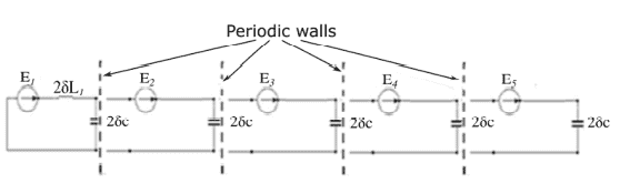
The traditional iterative wave method involves breaking down an electromagnetic problem into two parts $[\mathrm{BOZ} 09]$ as follows. The propagation equation aspect within a vacuum is dealt with in its entirety, and therefore translates as a relationship with the boundaries across sphere $D$, then with the boundary conditions running across sphere $D$. It is then necessary to have dual magnitudes linked together in a vacuum and at the boundaries, by linear operators, through a proportionality relationship (which is internal to $D$ ) and an integral relationship (which is external to $D$ ). Figure $1.3$ shows the unidimensional structure which is made up of several cells, each enclosed by periodic walls. This structure is periodic, except at source level. $$ E_{2}=E_{1} e^{j \alpha} ; E_{3}=E_{2} e^{j \alpha} ; E_{4}=E_{3} e^{j \alpha} ; E_{5}=E_{4} e^{j \alpha} $$
物理代写|电动力学代写electromagnetism代考|General Principles of the Wave Concept Iterative Process
The iterative method, which uses a wave network, is an integrated method and is not based upon electric and magnetic fields, as are, for example, Electrical Field Integral Equation (EFIE), Magnetic Field Integral Equation (MFIE), or more generally the method of moments or a combination of both fields. These are likened to the amplitudes of transverse waves, both diffracting around obstacles and those in space, termed “free space”, owing to the presence of evanescent fields. However, while the method of moments appeals to so-called admittance or impedance operators, within the wave iterative method (Wave Concept Iterative Process (WCIP)), the diffraction operators are restricted, thus leading to the convergence of all iterative processes based upon this particular formalism [BAU 99]
It may be noted that, with the method of moments, the solution to the problem often entails using a restriction in the given field so as to define trial functions that constitute the basis for given solutions. This often leads to both analytical and numerical problems. In the WCIP method, field conditions are simply described on the basis of pixels which make up the entire sphere.
Moreover, the iterative process has a significant resemblance to that used within harmonic equilibrium [KER 75]. Within this latter process the nonlinear component behaves in a way that is described in relation to time, while the rest of the circuit is described within the frequency sphere. The operator thus functions diagonally at given frequencies. With each iteration, we therefore proceed with a Fourier transform (using a time-frequency basis) so as to approach the detailed composition of boundary conditions at the shutdown level. Moreover, when writing equations in terms of components studied over time, an inverse Fourier transform (based upon frequency-time) is used.
The integral form of waves came to be explained during the $1990 \mathrm{~s}$, and was applied to planar circuits and to antennae [BAU 99, AZI 95, AZI 96, WAN 05, RAV 04, TIT 09]. The wave concept principle is as follows:
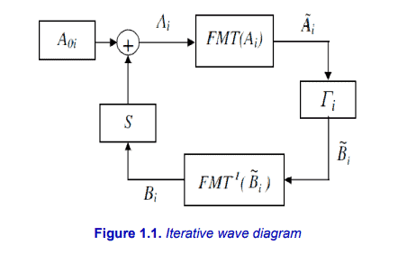
The electromagnetic issue may be expressed by the relationship between the two environments. The first is known as the spectral sphere or the external environment. The second is a set of surfaces which are defined by the boundary conditions at each point (termed the spatial domain). An Ao source in the spatial sphere sends a wave with an Ao amplitude towards a vacuum of free space. This wave is partly reflected (by the reaction of the operator $\Gamma$ ) and provides a wave $B$. The latter is, in its turn, reflected within the spatial sphere (the Operator S) giving us the wave $A$.
The $\Gamma$ operator is diagonal within the spectral sphere. It represents the homogeneous environment and its interaction with electromagnetic waves [BAU 99]. The operator $S$ describes the boundary conditions of the interface. It is expressed within the spatial sphere. The Fourier transform and its converse, the inverse Fourier transform, ensure the passage between both spheres. The relationships between incident and reflective waves are written as shown in [1.1] and [1.2]. $$ \begin{aligned} &\mathrm{B}=\Gamma \mathrm{A} \ &\mathrm{A}-\mathrm{SB}+\mathrm{A}_{0} \end{aligned} $$ With the first iteration, the spatial sphere equation should be expressed simply as Ao $(B=0)$. $B$ now appears with the operator $\Gamma(B=\Gamma A)$. The equation [1.2] is applied so as to obtain the new value of $A$ placed within [1.1], resulting in the new $B$ value. This iterative process consists in successively applying equations [1.1] and [1.2], until convergence occurs (Figure 1.1).
物理代写|电动力学代写electromagnetism代考|Introduction to ∫T(dXs)2 = t
The basis of traditional Itô calculus is the isometry property $\int_{\mathrm{T}}\left(d X_{s}\right)^{2}=t$. For this to be valid for Brownian motion $X=X_{\mathbf{T}}=\left(X_{s}: 0<s \leq t\right)$, and if an appropriate meaning or interpretation can be given to the “integral” expression of the isometry property, then the statement $\int_{T}\left(d x_{s}\right)^{2}=t$ must in some sense be valid for “typical” Brownian sample paths $x=x_{\mathbf{T}}=\left(x_{s}\right)$.
Traditional Itô calculus provides such an interpretation. The following discussion aims to provide a sense of what is involved.
In Example 24, every sample path $(x(s))$ satisfies $\int_{\mathrm{T}} d x_{s}=x_{t}$ provided the Stieltjes-complete definition of $\int_{T}$ is used. Examples in section $8.4$ of [MTRV] (pages 398-399) show that this approach does not work for $\int_{\mathbf{T}}\left(d x_{s}\right)^{2}$.
If $\int_{T}\left(d x_{s}\right)^{2}$ has some meaning as an integral then it is not unreasonable to seek to approximate it by means of some kind of Riemann sum expression of the form (N) $\sum\left(x_{s^{\prime}}-x_{s}\right)^{2},=\sum_{j=1}^{n}\left(x_{j}-x_{j-1}\right)^{2}$, where $N=\left{s_{1}, \ldots, s_{n-1}, s_{n}\right}$ is a partition of $\mathbf{T}=] 0, t]$ with $s=s_{j-1}<s_{j}=s^{\prime}, j=1, \ldots, n ; 0=s_{0}, s_{n}=t$. Such “typical” sample paths $\left(x_{s}\right)$ have unbounded variation (so the Lebesgue-style $\int_{0}^{t}\left|d x_{s}\right|$ typically diverges to $\left.+\infty\right)$. But ” $d x_{s}^{2}$ ” is typically less than $”\left|d x_{s}\right|$ “, so an aggregation of the form $\int_{0}^{t} d x_{s}^{2}$ may turn out to have a finite value. The expression $\sum_{j=1}^{n}\left(x_{j}-x_{j-1}\right)^{2}$ is a sample occurrence of a stochastic sum $f_{\mathrm{T}}^{g_{2}}\left(X_{\mathrm{T}}, \mathcal{N}\right)$ where the summand $g_{2}$ is $$ \left.\left.\left.\left.g_{2}\left(z_{s}\right)=\left(x\left(s^{\prime}\right)-x(s)\right)^{2} \text { for } \imath_{s}=\right] s, s^{\prime}\right], \quad x_{j}=\right] s_{j-1}, s_{j}\right], \quad x_{s_{j}}=x\left(s_{j}\right)=x_{j} . $$ For all partitions $N$ we have $$ X_{t}=\sum_{j=1}^{n}\left(X_{j}-X_{j-1}\right)=f_{\mathbf{T}}^{g_{1}}\left(X_{\mathbf{T}}, \mathcal{N}\right) $$ as in Example 24, and $$ \mathrm{E}\left[X_{t}\right]=\mathrm{E}\left[f_{\mathbf{T}}^{g_{1}}\left(X_{\mathbf{T}}, \mathcal{N}\right)\right]=\mathrm{E}\left[\sum_{j=1}^{n}\left(X_{j}-X_{j-1}\right)\right]=\sum_{j=1}^{n} \mathrm{E}\left[\left(X_{j}-X_{j-1}\right)\right]=0 $$ with $\mathrm{E}\left[\left(X_{j}-X_{j-1}\right)\right]=0$ for each $j$ since the increments of standard Brownian motion have mean 0. Again, according to the theory of Brownian motion the increments $X_{j}-X_{k}$ are independent for all choices of $j, k$, including $k=0$ and $j=n$, with variance $t_{j}-t_{k}$ in each case. Recall that, for any random variable $Y$, the variance $\operatorname{Var}[Y]$ is $\mathrm{E}\left[(Y-\mathrm{E}[Y])^{2}\right]$.
Some properties of finite-dimensional Gaussian integrals can be used to establish a version of the isometry property of Brownian motion.
P1 Assume $c<0$. Consider the one-dimensional integral $h(I)=\int_{u}^{v} y^{2} e^{c y^{2}} d y$ with $I$ a cell such as ] $u, v]$. In [MTRV] (page 263) integration by parts is applied, giving $$ \begin{aligned} \int_{u}^{v} y^{2} e^{c y^{2}} d y &=\frac{1}{2 c} \int_{u}^{v} y\left(e^{c y^{2}} 2 c y\right) d y \ &=\frac{1}{2 c}\left[y e^{c y^{2}}-\int e^{c y^{2}} d y\right]{u}^{v} \ &=\frac{1}{2 c}\left(v e^{c v^{2}}-u e^{c u^{2}}-\int{u}^{v} e^{c y^{2}} d y\right) \end{aligned} $$
P2 Suppose $x \in \mathbf{R}, f(x)=x^{2}$, and, for cells $\left.\left.I=\right] u, v\right]$ in $\mathbf{R}$, the cell function $g(I)$ is $\int_{I} e^{c y^{2}} d y$. For associated $(x, I)$ in $\mathbf{R}$, consider integrand $f(x) g(I)$ in domain $\mathbf{R}$. It is easy to show that $f(x) g(I)$ is variationally equivalent ${ }^{5}$ to $h_{0}(I)=\int_{u}^{v} y^{2} e^{c y^{2}} d y$. Since the latter is an additive cell function, it is the indefinite integral ${ }^{6}$ of the integrand $f(x) g(I)$; and, by the preceding calculation, the indefinite integral of $f(x) g(I)$ can be expressed as the additive cell function $$ h_{0}(I)=\frac{1}{2 c}\left(v e^{c v^{2}}-u e^{c u^{2}}-\int_{u}^{v} e^{c y^{2}} d y\right) $$ The purpose of presenting the indefinite integral of integrand $x^{2} \int_{I} e^{c y^{2}} d y$ in the form $(6.8)$ is to establish the isometry property of Brownian motion. P3 Next, consider finite-dimensional domain $\mathbf{R}^{m}$ with points and cells $$ x=\left(x_{1}, \ldots, x_{m-1}, x_{m}\right), \quad I=I_{1} \times \cdots \times I_{m-1} \times I_{m}, $$ respectively. Let $h_{1}(I)=$ $$ =\int_{I}\left(y_{1}^{2}+\cdots+y_{m-1}^{2}+y_{m}^{2}\right) e^{\left(c_{1} y_{1}^{2}+\cdots+c_{m-1} y_{m-1}^{2}+c_{m} y_{m}^{2}\right)} d y_{1} \ldots d y_{m-1} d y_{m} $$ if the integral exists. Assume $c_{j}<0$ for $j=1 \ldots, m$. Regarding existence, for any $k(1 \leq k \leq m)$, with $\left.\left.I_{k}=\right] u_{k}, v_{k}\right],(6.8)$ implies $$ \begin{aligned} & \int_{I}\left(y_{k}^{2} e^{\sum_{j=1}^{m} c_{j} y_{j}^{2}}\right) d y_{1} \ldots d y_{m}=\ =& \int_{I_{k}} y_{k}^{2} e^{c_{k} y_{k}^{2}} d y_{k} \prod\left(\int_{I_{j}} e^{c_{j} y_{j}^{2}} d y_{j}: j=1,2, \ldots, m, j \neq k\right) \ =& \frac{1}{2 c_{k}}\left(v_{k} e^{c_{k} v_{k}^{2}}-u_{k} e^{c_{k} u_{k}^{2}}-\int_{I_{k}} e^{c_{k} y^{2}} d y_{k}\right) \prod_{j \neq k}\left(\int_{I_{j}} e^{c_{j} y_{j}^{2}} d y_{j}\right) \end{aligned} $$ so the first integral $\int_{I} \cdots$ exists. Thus $h_{1}(I)=$ $$ =\sum_{k=1}^{m}\left(\frac{1}{2 c_{k}}\left(v_{k} e^{c_{k} v_{k}^{2}}-u_{k} e^{c_{k} u_{k}^{2}}-\int_{I_{k}} e^{c_{k} y_{k}^{2}} d y_{k}\right) \prod_{j \neq k}\left(\int_{I_{j}} e^{c_{j} y_{j}^{2}} d y_{j}\right)\right) $$ and $h_{1}(I)$ is finitely additive on disjoint cells $I$. This ensures that $h_{1}(I)$ is integrable on $\mathbf{R}^{m}$. Now define $h(I):=$ $$ :=h_{1}(I) \prod_{j=1}^{m}\left(\frac{\pi}{-c_{j}}\right)^{-\frac{1}{2}}=\int_{I_{1} \times \cdots \times I_{m}}\left(\sum_{j=1}^{m} y_{j}^{2} e^{\sum_{j=1}^{m} c_{j} y_{j}^{2}}\right) \frac{d y_{1}}{\sqrt{\frac{\pi}{-c_{1}}}} \cdots \frac{d y_{m}}{\sqrt{\frac{\pi}{-c_{m}}}} $$
(where $\int_{\mathbf{R}} e^{c_{j} y_{j}^{2}} \frac{d y_{j}}{\sqrt{\frac{\pi}{-c_{j}}}}=1$ for each $j$ by theorem 133, [MTRV] page 261). Note that each of $v_{k} e^{c_{k} v_{k}^{2}}$ and $u_{k} e^{c_{k} u_{k}^{2}}$ tends to zero as $\left|v_{k}\right|,\left|u_{k}\right|$ tend to infinity. Therefore, using the -complete integral construction on $\mathbf{R}$ ([MTRV] pages 69-78, corresponding to improper Riemann integration), $$ \int_{\mathbf{R}^{m}} h(I)=h\left(\mathbf{R}^{m}\right)=\sum_{k=1}^{m} \frac{-1}{2 c_{k}} . $$
物理代写|电动力学代写electromagnetism代考|Isometry Property for Stochastic Sums
The second integrand/summand in the lists $(5.31)$ and $(5.32)$ is the function $g_{2}$. By adding more detail to Section $6.5$ the formulation $\int_{0}^{t} d X_{s}^{2}=t$ can now be brought into a framework of stochastic sums.
In $(6.7)$ the partition points $\tau_{j}$ of $M$ are taken to be fixed times for the purpose of calculating the expected value $\mathrm{E}\left[\sum_{j=1}^{m}\left(X_{j}-X_{j-1}\right)^{2}\right]$ in a finitedimensional sample space $\mathbf{R}^{M}$, with $M=\left{\tau_{1}, \ldots, \tau_{m-1}, \tau_{m}\right}$. In contrast, Sections $6.3$ and $6.4$ have provided expressions such as $\sum_{j=1}^{n}\left(X_{j}-X_{j-1}\right)^{2}$ in equation (6.7) with an enhanced meaning as a new kind of observable or random
variable, $$ f_{\mathbf{T}}^{g_{2}}\left(X_{\mathbf{T}}, \mathcal{N}\right)=\sum_{j=1}^{n}\left(X_{j}-X_{j-1}\right)^{2} . $$ Here, $f_{\mathbf{T}}^{g_{2}}\left(X_{\mathbf{T}}, \mathcal{N}\right)$ is an observable in sample space $\mathbf{R}^{\mathbf{T}}$ with distribution function $G(I[N])$ for times $N \subset \mathbf{T}$ : $$ \mathscr{f}{\mathbf{T}}^{g{2}}\left(X_{\mathbf{T}}, \mathcal{N}\right) \simeq \mathscr{f}{\mathbf{T}}^{g{2}}\left(x_{\mathbf{T}}, N\right)\left[\mathbf{R}^{\mathrm{T}}, G\right] $$ in which $N$ is variable, so sample values $f_{\mathbf{T}}^{g_{2}}\left(x_{\mathbf{T}}, N\right)$ are constructed from samples of times $s_{j} \in N \subset \mathbf{T}$, with corresponding sample values $x_{j},=x\left(s_{j}\right)$ of the random variables $X_{j},=X\left(s_{j}\right)$, of the process $X_{\mathbf{T}}$.
If observable $f_{\mathbf{T}}^{g_{2}^{2}}\left(X_{\mathbf{T}}, \mathcal{N}\right)$ has expected value it is a random variable. And, in that case, it is an absolute random variable (and therefore measurable) since its sample values are non-negative. (See theorems 76 and 250 , [MTRV] pages 193 and 494.) Example 25 below confirms these properties, with $$ \mathrm{E}\left[f_{\mathbf{T}}^{g_{2}}\left(X_{\mathbf{T}}, \mathcal{N}\right)\right]=\int_{\mathbf{R}^{\mathbf{T}}}\left(f_{\mathbf{T}}^{g_{2}}\left(x_{\mathrm{T}}, N\right)\right) G(I[N])=t $$ Thus $$ f_{\mathbf{T}}^{g_{2}}\left(X_{\mathbf{T}}, \mathcal{N}\right), \quad=\sum_{s_{j} \in N}\left(X\left(s_{j}\right)-X\left(s_{j-1}\right)\right)^{2} \text { with variable } N \in \mathcal{N}, $$ is the meaning we ascribe to $\int_{\mathrm{T}} d X_{s}^{2}$, validating the latter as a random variable contingent on the Brownian process $X_{\mathbf{T}}$, so $$ \mathrm{E}\left[\int_{\mathbf{T}} d X_{s}^{2}\right]=\int_{\mathbf{R}^{\mathbf{T}}}\left(\int_{\mathrm{T}} d x_{s}^{2}\right) G(I[N])=t . $$ In this way, Example 25 supports the traditional Itô calculus interpretation of ” $\int_{\mathrm{T}} d X_{s}^{2} “$ as a weak integral which converges “in the mean” to value $t$.
物理代写|电动力学代写electromagnetism代考|Riemann Sums for Stochastic Integrals
This section seeks to extend the Riemann sum stratagem described above in order to simplify and unify various conceptions of strong and weak stochastic integration; and to replace stochastic integrals by stochastic sums.
A stochastic process is a family of random variables $X=X_{\mathbf{T}}=\left(X_{s}\right), s \in \mathbf{T}$, where $\mathbf{T}$ is an infinite set such as $] 0, t]$. Stochastic integration is a device which constructs a random variable $Z$ from a process $X_{\mathrm{T}}$; such as $$ Z=\int_{0}^{t} X_{s} d X_{s} . $$ Example 23 Constructions of this kind have been given a variety of interpretations and meanings in chapter 8 (pages 383-446) of [MTRV], such as strong and weak stochastic integrals: $$ \mathbf{S}{T}^{g}\left(X{\mathbf{T}}\right), \quad \mathcal{S}{\mathbf{T}}^{g}\left(X{\mathrm{T}}\right) $$ where (in this case) the integrand $g$ is $X_{s}\left(X_{s^{\prime}}-X_{s}\right),=X_{s} d X_{s},\left(0 \leq s<s^{\prime} \leq t\right)$. In fact, provided $X_{\mathbf{T}}$ is standand Brownian motion, $\int_{0}^{t} X_{s} d X_{s}$ is $\mathcal{S}{\mathrm{T}}^{g}\left(X{\mathrm{T}}\right), a$
weak stochastic integral which evaluates as $\frac{1}{2} X_{t}^{2}-\frac{1}{2} t . \quad$ (See example 63 , pages $405-406$ of [MTRV].)
Expressed in terms of sample values $x_{s}(0<s<t)$, or in terms of sample path $x_{T}$, this result states that, with $x_{t}=x(t)$ given, $$ \mathcal{S}{T}^{g}\left(x{T}\right)=\int_{0}^{t} x_{s} d x_{s}=\int_{0}^{t} x(s) d x(s)=\frac{1}{2} x_{t}^{2}-\frac{1}{2} t $$ in some weak sense; where $\int_{0}^{t} x(s) d x(s)$ is a Stieltjes-type integral of the pointfunction $x(s)$ with respect to (increments of) the point-function $x(s)$. (a) Equation (6.4) is a “weak” equation, which can only be valid in some sense of “average value” of one or other side, or both. (b) Furthermore, the left hand side of (6.4) references infinitely many values $x_{s}$, corresponding to the infinitely many time instants $0<s<t . A s$ in (6.3), this suggests infinitely many sample measurements $x_{s}$. This is counter-intuitive as a method of calculation. It is not practically possible to sample every instant s of time.
In the discussion below, both of these issues are addressed by using (as in (6.4)) a Riemann sum method for the averaging required by (a), so each Riemann sum involves a finite sample consisting of only a finite number of times s.
物理代写|电动力学代写electromagnetism代考|Stochastic Sum as Observable
A new type of observable is required: $$ f\left(X_{\mathbf{T}}, \mathcal{N}\right) \simeq f\left(x_{\mathbf{T}}, N\right)\left[\mathbf{R}^{\mathbf{T}}, F_{X_{\mathbf{T}}}\right] $$ where $F_{X_{\mathbf{T}}}$ is a distribution function defined for $I[N] \in \mathcal{I}\left(\mathbf{R}^{\mathbf{T}}\right.$ ) (the set of cells in $\left.\mathbf{R}^{\mathbf{T}}\right)$ $$ F_{X_{\mathrm{T}}}: \mathcal{I} \mapsto[0,1], \quad 0 \leq F_{X_{\mathrm{T}}}(I[N]) \leq 1 . $$ In addition to dependence on joint occurrences $\left(x_{s}\right)=x_{\mathbf{T}}$, an observable $f$ is permitted to depend explicitly on partitions $N=\left{s_{1}, \ldots, s_{n-1}, s_{n}\right}$ of $\mathbf{T}$. Likewise, a distribution function $F_{X_{\mathrm{T}}}$ depends on cells $I=I[N]$, and may depend explicitly on the partitions $N=\left{s_{1}, \ldots, s_{n-1}, s_{n}\right}$ of T which (with $s_{n}=t$ ) are the “cylinder labels”, or dimension labels, of the cylindrical intervals $I[N]$ in $\mathbf{R}^{\mathbf{T}}$. For example, with $\left.\left.I_{t}=\right] u_{t}, v_{t}\right](t \in N)$, the incremental Gaussian distribution function $G$ of (5.8) (see page 115 above) depends explicitly on the parameters $u_{t}, v_{t}$, and $t$, for $t \in N$.
A left hand limit (or vertex) $u_{t}$ for a partitioning component cell $\left.I_{t}=\right] u_{t}, v_{t}$ ] $(t \in N)$ is a right hand limit or vertex of an adjoining cell $I_{t}^{\prime}$. Thus, choice of a partition $\mathcal{P}$ of domain $\mathbf{R}^{\mathbf{T}}$ reduces to choice of finite samples $N$ of times, along with choices $\left{u_{t}\right}$ of finite samples of vertices for $t \in N$.
As outlined in Section $6.2$, the fundamental step is to define the expectation $\mathrm{E}\left[f\left(X_{\mathrm{T}}, \mathcal{N}\right)\right]$; that is, to define the integral of $f\left(x_{\mathrm{T}}, N\right)$ with respect to distribution function $F(I[N])$. In particular, when $f\left(x_{\mathbf{T}}, N\right)=\mathcal{R}{\mathbf{T}}^{g}\left(x{\mathbf{T}}, N\right)$, (or $\left.f_{\mathbf{T}}^{g}\left(x_{\mathbf{T}}, N\right)\right)$ $$ \begin{aligned} \mathrm{E}\left[\mathcal{R}{\mathbf{T}}^{g}\left(X{T}, \mathcal{N}\right)\right], &=\int_{\mathbf{R}^{\mathbf{T}}}\left(\mathcal{R}{\mathbf{T}}^{g}\left(x{\mathbf{T}}, N\right)\right) F(I[N]), \ \text { or } \mathrm{E}\left[\oiint_{\mathbf{T}}^{g}\left(X_{\mathbf{T}}, \mathcal{N}\right)\right], &=\int_{\mathbf{R}^{\mathrm{T}}}\left(\oiint_{\mathbf{T}}^{g}\left(x_{\mathbf{T}}, N\right)\right) F(I[N]) \end{aligned} $$ so $f_{\mathrm{T}}^{g}\left(X_{\mathbf{T}}, \mathcal{N}\right.$ ) is a random variable. Chapter 4 (pages 111-182) of [MTRV] deals with the integration in $\mathbf{R}^{S}$ of integrands of the form $h\left(x_{S}, N, I[N]\right)$, where $S$ is any infinite set (such as intervals of time $\mathbf{T}$ or $T$ ), including integrands $f\left(x_{S}, N\right) F(I[N])$. Briefly, $f\left(x_{S}, N\right) F(I[N])$ is integrable on $\mathbf{R}^{S}$, with integral $$ \int_{\mathbf{R}^{S}} f\left(x_{S}, N\right) F(I[N])=\alpha, $$ if, given $\varepsilon>0$, there exists a gauge $\gamma=\left(L, \delta_{\mathcal{N}}\right)$ such that, for every $\gamma$-fine division $\mathcal{D}$ of $\mathbf{R}^{S}$, the corresponding Riemann sums satisfy $$ \left|\alpha-(\mathcal{D}) \sum f\left(x_{S}, N\right) F(I[N])\right|<\varepsilon $$ Chapter 4 of [MTRV] provides a theory of variation for functions $h(x, N, I[N])$ which is applicable to functions $F(I[N])$ and $f(x, N) F(I[N])$. So, for instance, $F(I[N]$ ) (defined on cells $I[N])$ can be extended to an “outer measure” on arbitrary subsets $A$ of $\mathbf{R}^{S}$. Chapter 4 also provides limit theorems for integrals (such as integrability of limits of integrable functions), and Fubini’s theorem for integrands defined on product domains of the form $\mathbf{R}^{S^{\prime}} \times \mathbf{R}^{S^{\prime \prime}}$.
物理代写|电动力学代写electromagnetism代考|Stochastic Sum as Random Variable
This section follows through on the definitions of Section 6.3, using familiar examples to illustrate the theory of stochastic sums, as replacement for both strong and weak stochastic integrals in chapter 8 of [MTRV]. The examples are based on the functions $g_{1}$ to $g_{9}$ of pages 391-392; also listed in (5.31) and (5.32) at the end of Chapter 5 above.
The notation is as set out in section $8.2$ of MTRV (pages $386-390$ ); with
$\mathbf{T}=] 0, t]$ replacing the symbol $\mathcal{T}=] 0, t]$ of $[\mathrm{MTRV}] .$ For any given $x_{\mathbf{T}} \in \mathbf{R}^{\mathbf{T}}$, $$ \begin{aligned} z_{s} &\left.=] s, s^{\prime}\right], & & 0 \leq s<s^{\prime} \leq t, \ \mathbf{x}\left(z_{s}\right) &=x\left(s^{\prime}\right)-x(s), & & x=x_{\mathrm{T}} \in \mathbf{R}^{\mathrm{T}}, \ g &=g\left(x_{s}, s, \mathbf{x}\left(z_{s}\right), z_{s}\right), & & \text { a stochastic summand (or integrand), } \ \mathbf{X}\left(z_{s}\right) &=X\left(s^{\prime}\right)-X(s), & & X=X_{\mathrm{T}} \text { an observable in sample space } \mathbf{R}^{\mathrm{T}}, \ N &=\left{s_{1}, \ldots, s_{n-1}, s_{n}\right}, & & \text { a partition of } \mathbf{T}, \text { or finite subset of } \mathbf{T}, \ z_{j} &\left.=] s_{j-1}, s_{j}\right], & j=1, \ldots, n, \quad s_{0}=0, s_{n}=t . \end{aligned} $$ For $g=g_{1}, \ldots, g_{9}$ of $(8.16)$ in page 419 of [MTRV], evaluations of stochastic integrals (strong and weak) have been given in [MTRV]. The idea here is to illustrate stochastic summation by replacing ${ }^{4}$ the stochastic integrals $\mathbf{S}{\mathbf{T}}^{g{j}}\left(X_{\mathbf{T}}\right)$ or $\mathcal{S}{\mathbf{T}}^{g{j}}\left(X_{\mathbf{T}}\right)$ with corresponding stochastic sums of the form $$ \int_{\mathbf{T}}^{g_{j}}\left(X_{\mathbf{T}}, \mathcal{N}\right)=\sum_{j=1}^{n} g_{j}\left(X_{s_{j}}, s_{j}, \mathbf{X}\left(z_{s_{j}}\right), z_{s_{j}}\right) $$
物理代写|电动力学代写electromagnetism代考|Varieties of Stochastic Integral
This section provides a summary and overview of stochastic integrals. The notation for stochastic integrals in a Riemann setting is set out in section $8.2$ (pages $386-390$ ) of [MTRV]. The family of cells or intervals in a domain $\Omega$ is denoted by $\mathcal{I}(\Omega)$. So if $\Omega$ is, respectively, a real interval such as $] 0, t]$, a finitedimensional domain $\mathbf{R}^{M}$, or an infinite-dimensional domain $\mathbf{R}^{] 0, t]}$, then $\mathcal{I}(\Omega)$ consists of cells which are denoted, respectively, by $$ \text { 2, } I(M), \quad I[N], $$ where $M$ and $N$ are finite sets. For ease of reference, relevant content of section $8.2$ of [MTRV] is repeated here.
Suppose $\left.\mathbf{T}=] \tau^{\prime}, \tau\right]$ (closed on the right) and suppose $F_{X},=F_{X_{T}}$, is a distribution defined on $\mathcal{I}\left(\mathbf{R}^{\mathrm{T}}\right)$; so $X \simeq x\left[\mathbf{R}^{\mathrm{T}}, F_{X}\right]$ is a joint-basic observable.
Suppose $\left.\left.2,=i_{s},=\right] s, s^{\prime}\right] \in \mathcal{I}(\mathbf{T})$ and $f\left(x,\left{s, s^{\prime}\right}\right)=x\left(s^{\prime}\right)-x(s)=\mathbf{x}\left(\imath_{s}\right)$. We then have a contingent joint observable $$ f\left(X,\left{s, s^{\prime}\right}\right) \simeq f\left(x,\left{s, s^{\prime}\right}\right)\left[\mathbf{R}^{\mathbf{T}}, F_{X}\right], \quad \text { or } \quad \mathbf{X}\left(\imath_{s}\right) \simeq \mathbf{x}\left(\imath_{s}\right)\left[\mathbf{R}^{\mathbf{T}}, F_{X}\right] . $$ Suppose $g$ is a function of the elements $\mathbf{x}(\imath)$ for $\imath \in \mathcal{I}(\mathbf{T})$. For instance, $g(\mathbf{x}(\imath))$ could be the function $$ g(\mathbf{x}(2)),=g\left(\mathbf{x}\left(z_{s}\right)\right),=\mathbf{x}\left(z_{s}\right)^{2}=\left(x\left(s^{\prime}\right)-x(s)\right)^{2} . $$ The family of finite subsets of $\mathbf{T}$ is denoted by $\mathcal{N}(\mathrm{T})$. If $N=\left{t_{1}, t_{2}, \ldots, t_{n}\right} \in$ $\mathcal{N}(\mathrm{T})$ with $t_{0}=\tau^{\prime}$ and $t_{n}=\tau$, we $\operatorname{can}^{13}$ write $\left.\left.\imath_{j}=\right] t_{j-1}, t_{j}\right]$. Thus the cells $\left{\imath_{j}\right}$ form a partition of the domain $\mathbf{T}$. For simplicity, let the symbol $N$ denote:
partition points $\left{t_{j}\right}$, or
partition $\left{z_{j}\right}$, or
division $\left.\left.\left{(\bar{s},] t_{j-1}, t_{j}\right]\right)\right$,$} , with associated points (or tag points) \bar{s}=t_{j-1}$ or $\bar{s}=t_{j} \cdot$
物理代写|电动力学代写electromagnetism代考|Stochastic Sums
In Chapter 1 the classical or standard concept of stochastic integral, including Itô’s integral, is outlined. The mathematical need or motive for some concept of stochastic integration has been illustrated in preceding chapters by means of various examples. It is illustrated in particular by the manifestation, in the form of a stochastic integral, of the value at any time $t$ of a shareholding (or portfolio) of a quantity $g(s)$ of shares whose value at time $s(0 \leq s \leq t)$ is $x(s)$ : $$ \int_{0}^{t} g(s) d x(s), $$ where $g(s)$ is a deterministic or random function of time $s(0 \leq s \leq t)$ and $x(s)$ $(0<s \leq t)$ is a sample path of a process $X=\left(X_{s}\right)_{0<s \leq t^{*}}$
The latter expression $\mathcal{S}{\mathrm{T}}^{g}(X)$ corresponds to the classical $\int{0}^{t} g(s) d X(s)$ (which is the Itô integral if $\left(X_{s}\right)$ is a Brownian motion). The other three expressions are innovations. They are introduced in MTRV, which includes discussion of $\mathbf{s}{\mathrm{T}}^{g}(X)$ and $\mathbf{S}{\mathrm{T}}^{g}(X)$, along with a brief outline of the first one, $\mathcal{R}_{\mathrm{T}}^{g}(X, N)$.
In mathematical discussion of integration, including stochastic integration, it is customary to use a notation with three components ${$ integral symbol $}{$ point integrand $}{$ differential $}$ or $\left(\int\right)(f(y))(d y)$. In the -complete integration of [MTRV], this is expressed as $\int f(y) k(I)$, where $k(I)=|I|$ corresponds to the traditional differential symbol $d y$.
Traditionally, a stochastic integral may take the form $\int f(X) d X$ where $X$ is a stochastic process. But [MTRV] breaks with this notation. Instead of $\int$ we have symbols s, $\mathbf{S}$, and $\mathcal{S}$; each used in particular contexts (see section 8.2, [MTRV] pages $386-390)$. Integrand elements such as $f(X) d X$ are denoted by some expression $g$ which is attached to the relevant integration symbol as a superscript, giving $$ \mathbf{s}^{g}, \quad \mathbf{S}^{g}, \quad \mathcal{S}^{g} . $$ [MTRV] also introduces another such functional, $\mathcal{R}^{g}$, which is a Riemann sum rather than an integral, and which is now to be written $f^{g}$.
As well as integration, these procedures have a functional aspect, in the sense that the final result depends on the choice of sample path $x_{T}$. The innovations in notation are intended to emphasize the functional rather than the integration aspect. So with the integrand $g$ safely relegated to superscript position, the functional dependence on $x_{\mathbf{T}}$ is denoted by $$ \mathbf{s}^{g}\left(x_{\mathbf{T}}\right), \quad \mathbf{S}^{g}\left(x_{\mathrm{T}}\right), \quad \mathcal{S}^{g}\left(x_{\mathrm{T}}\right) $$ and, whenever needed for clarity, the domain $\mathbf{T}$ is placed as subscript, $$ \mathbf{s}{\mathbf{T}}^{g}\left(x{\mathbf{T}}\right), \quad \mathbf{S}{\mathbf{T}}^{g}\left(x{\mathrm{T}}\right), \quad \mathcal{S}{\mathbf{T}}^{g}\left(x{\mathbf{T}}\right), $$ just as it is in $\int_{T}$. The same general idea is in the stochastic sum notation $$ \mathcal{R}{\mathbf{T}}^{g}\left(x{\mathbf{T}}\right), \quad \mathcal{f}{\mathbf{T}}^{g}\left(x{\mathbf{T}}\right) $$ These two symbols are equivalent, but the latter symbol is given precedence because of the suggestion it contains of “sum replacing integral”.
The aim of this chapter is to amplify and extend the ideas behind $\mathcal{R}{T}^{g}(X)-$ or $\mathcal{R}{\mathrm{T}}^{g}(X, \mathcal{N})$, or $\xi_{\mathbf{T}}^{g}\left(X_{\mathbf{T}}, \mathcal{N}\right)$-as a simpler and more comprehensive way of dealing with stochastic integration; so that the single formulation $f_{\mathbf{T}}^{g}\left(X_{\mathbf{T}}, \mathcal{N}\right)$ replaces each of $\mathbf{s}{\mathbf{T}}^{g}(X), \mathbf{S}{\mathbf{T}}^{g}(X), \mathcal{S}{\mathbf{T}}^{g}(X)$, and $\int{\mathbf{T}} f(X) d X$.
物理代写|电动力学代写electromagnetism代考|Review of Random Variability
To set the scene for this, here is an overview of the -complete approach to random variability, with emphasis on those aspects which reinforce and validate the replacement of stochastic integrals by stochastic sums.
Random variability is associated with observation or measurement of some quantity whose precise value is not known, but for which estimated values $x$ can be given. Suppose that, even though the precise or true value is not known, there is some method of assessing the accuracy of estimated values $x$. Suppose, in fact, that the degree or level of accuracy of the estimate $x$ can itself be estimated by means of a distribution function $F$ or $F_{X}$ defined on intervals $I$ of possible values of $x$ in domain $\Omega$ (called the sample space). Then the term observable is applied to the notion of measurement or estimate $X$, with possible values $x$ in sample space $\Omega$, equipped with accuracy function (or likelihood distribution function) $F_{X}$. $$ X \simeq x\left[\Omega, F_{X}\right] . $$ The measured value (or occurrence, or datum) $x$ can be a number (usually real), so $\Omega=\mathbf{R}$. Or $x$ can consist of jointly measured values $x=\left(x_{s}\right)$ where $s \in \mathbf{T}$; so if $\mathbf{T}$ is a finite set of cardinality $n$, then $\Omega=\mathbf{R}^{n}$ and $x=\left(x_{1}, \ldots, x_{n}\right)$. In that case, $X \simeq x\left[\mathbf{R}^{n}, F_{X}\right]$ is a joint-basic observable, with distribution function $F_{X}$ defined on cells $$ I=I_{1} \times \cdots \times I_{\mathrm{n}} \subset \mathbf{R}^{n}, \quad x_{j} \in I_{j}, \quad j=1, \ldots n . $$ If the measurement is a real value $f(x)$ formed by means of a deterministic function $f$ of the basic observable $x$, then $f(X)$ is a contingent observable $$ f(X) \simeq f(x)\left[\Omega, F_{X}\right] . $$ An event is a set of occurrences. An observable $f(X)$ is a random variable (or is an $F_{X}$-random variable) if its expected value $\mathrm{E}[f(X)]$ exists: $$ \mathrm{E}[f(X)]=\int_{\Omega} f(x) F_{X}(I) . $$
物理代写|电动力学代写electromagnetism代考|Review of Brownian Probability
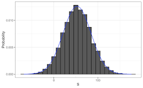
About half of [MTRV] is taken up with $(5.8),(5.12)$, and related expressions. When motivational and explanatory material is included, these expressions, along with their properties and implications, constitute almost all of the present
book whenever the Feynman quantum mechanical expression (8.29) of Section $8.6$ below is included. [MTRV] uses the symbol $\mathcal{G}$ for geometric Brownian distribution function (5.12). while the symbol $G_{c}(I[N])$ is used to denote the joint distribution function for $c$-Brownian motion. So $G_{-\frac{1}{2}}$ gives standard or classical Brownian motion (5.8); while $G_{\frac{1}{2}}$ is used in [MTRV] for the Feynman theory of (8.29). But in this book the symbol $G$ is used without subscript, allowing the context (Brownian motion or quantum mechanics) to show which meaning is intended. To sum up, the theory of $(5.8),(5.12)$, and $(8.29)$ is covered in chapters 6,7 , and 8 of [MTRV]. It is not proposed to rehearse this theory here; but, instead, to highlight some aspects of it which are particularly relevant to the topics of this book.
In [MTRV], Brownian motion, geometric Brownian motion, and Feynman path integration (for single particle mechanical phenomena) are united in a single theory based on a version of Fresnel’s integral using a parameter $c=a+\iota b$, where $\iota=\sqrt{-1}, a \leq 0$, and $c \neq 0$ (so $a$ and $b$ are not both zero.)
The case $c=-\frac{1}{2}$ (real, negative) leads to Brownian and geometric Brownian motion. The case $c=\frac{\sqrt{-1}}{2}$ (pure imaginary) gives Feynman path integrals. The designation $c$-Brownian motion is intended to cover all cases, including those which are “intermediate” between real negative and pure imaginary.
The Fresnel evaluation is in theorem 133 (pages 261-262 of [MTRV]). For $c<0$ (real, negative) lemmas 12 and 13 (page 262) show that finite compositions (or addition) of normal distributions are normal, so that these distributions are additive in some sense. And provided the real part of $c$ is non-positive (with $c \neq 0$ ), lemmas 12 and 13 are valid for complex-valued $c$.
These results are crucial in going from finite compositions of distributions to infinite compositions, giving a theory of infinitely many (and “infinitely divisible” ${ }^{n}$ or continuum) of normal distributions (or c-normal distributions), leading to the theory of $c$-Brownian motion.
Joint probability distributions are defined on domains $\mathbf{R}^{\mathbf{T}}$ where $\mathbf{T}$ is typically a real interval open on the left and closed on the right, such as $$ ] 0, t], \quad] 0, \tau], \quad] \tau^{\prime}, \tau\right] \text {. } $$ A joint distribution such as $(5.8),(5.12)$, or $(8.29)$, is constructed for samples $$ N=\left{t_{1}, t_{2}, \ldots, t_{n-1}, t_{n}\right} \subset \mathbf{T} $$ with $t_{0}$ taken to be the left hand boundary of interval $\mathbf{T}$, and $t_{n}$ the right hand boundary point.
A stochastic integral with respect to Brownian processes can have forms $$ \int_{0}^{t} g(s) d X(s), \quad \int_{0}^{t} f(X(s)) d X(s), \quad \int_{0}^{t} Z(s) d X(s) . $$ Each random variable $X(s)(0<s \leq t)$ is normally distributed, so individually they are not too difficult.
But $\int_{0}^{t}$ involves a continuum of such normal distributions. Section $4.4$ mentions step functions, cylinder functions, and sampling functions as a progression of stages in dealing with this problem. This section applies a cylinder function approach to Brownian stochastic integrals. The idea is to replace the continuum ] $0, t]$ by discrete times $0=\tau_{0}<\tau_{1}<\cdots<\tau_{n}=t$. (In Part II, R. Feynman’s path integrals of cylinder functions use a countable infinity of discrete times $\tau_{j}$-) For $0<t \leq \tau$ let $\mathbf{T}$ denote $] 0, t]$, closed at boundary $t$; and let $T$ denote $] 0, t[$, open at boundary $t$. Suppose an asset price process $X_{T}$ can be represented as $$ X_{\mathrm{T}} \simeq x_{\mathrm{T}}\left[\mathbf{R}^{\mathbf{T}}, G\right] $$
where $x(0)=0$ for all sample paths, and $G$ is the joint probability distribution function $G(I[N])$ of $(5.8)$ for standard Brownian motion. Assume the asset is some portfolio which (unlike shares) can take unbounded positive and negative values. In other words the “asset” (or portfolio) can also be a liability.
A distinction can be made between the value of the portfolio at any time $t$, and the earnings of the portfolio at time $t$.
The latter is intended to denote the stake of the investor or holder of the portfolio, taking account of the initial expenditure (denoted below by $\beta$ ) paid out by the investor in order to acquire possession of the portfolio to begin with. The former represents a third party view of the portfolio, disregarding any cost of acquisition. If $w(t)$ is the value of the portfolio then earnings equal $w(t)-\beta$ for all $t$; where $\beta$ denotes the upfront cost to the investor of acquiring the portfolio at time $t=0$.
The value of the portfolio at any time $s$ depends on the size $\nu(s)$ of (or number of units of the assets/liabilities in) the portfolio. Then the value of the portfolio at time $s$ is $\nu(s) x(s)$. For the purpose of investigating stochastic integrals, the number $\nu(s)$ can have various interpretations, such as $$ g(s), \quad Z(s), \quad f(X(s)) $$ where, for $0 \leq s \leq t, g(s)$ is a deterministic 4 function, $(Z(s))$ is a random process independent of the Brownian motion $(X(s))$, and $(f(X(s)))$ is a process which depends on $(X(s))$.
物理代写|电动力学代写electromagnetism代考|Some Features of Brownian Motion
Example 19 above suggests there is a need to consider some extreme behaviour of Brownian paths.
Mathematical Brownian motion is very “bad”. A stereotypical pictorial representation of a sample element of Brownian motion is a “jagged-path” graph consisting of straight line segments adjoining each other consecutively with sharp corners at the points where each one adjoins the next one.
Mathematically, however, a typical sample path is nowhere differentiable. This is much “worse” than the jagged-path graphical representation. Except for their end points, line segments are smooth, or differentiable. So the class of all such jagged paths are a $G$-null subset of the sample space $\Omega=\mathbf{R}^{\mathbf{T}}$.
The reason for this “badness” is that, typically, the increments or transitions $x\left(s^{\prime}\right)-x(s)$ vary as the square root of the time increment $s^{\prime}-s$. Calculating a derivative for $x(s)$ at $s$ involves $$ \frac{x\left(s^{\prime}\right)-x(s)}{s^{\prime}-s}=\frac{1}{\sqrt{s^{\prime}-s}}\left(\frac{x\left(s^{\prime}\right)-x(s)}{\sqrt{s^{\prime}-s}}\right) $$ which diverges as $s^{\prime} \rightarrow s$ for “typical” $x$ of Brownian motion, since the final factor remains finite for such $x$.
From a different perspective, mathematical Brownian motion is very “good”. This is because, typically ${ }^{10}$, its sample paths are uniformly continuous. The reason for this “goodness” is that, typically, the increments or transitions $x\left(s^{\prime}\right)$ $x(s)$ vary as the square root of the time increment $s^{\prime}-s$. So if $s^{\prime} \rightarrow s$ then $\sqrt{s^{\prime}-s} \rightarrow 0$ and hence $x\left(s^{\prime}\right) \rightarrow x(s) .$
These issues are discussed in detail in chapter 6 of [MTRV], and in many other presentations of the subject
Brownian motion includes sample paths which resemble the Dirichlet function of Example 13, and it includes straight lines, and it includes everything in between these two extremes.
In this book stochastic integrals have been presented as some kind of Stieltjes integral, involving integration of one point function $h_{1}(s)$ with respect to a different point function $h_{2}(s)$. (In Section $5.4$ the integrator function $h_{2}\left(s^{\prime}\right)$ $h_{2}(s)$ was supposed to be a Brownian sample path increment $x\left(s^{\prime}\right)-x(s)$; while the integrand function $h_{1}(s)$ was generally designated as $g(s)$.)
A basic Riemann-Stieltjes integral has Riemann sum approximations of the form $$ \sum h_{1}\left(s^{\prime \prime}\right)\left(h_{2}\left(s^{\prime}\right)-h_{2}(s)\right) $$ where $s^{\prime \prime}$ satisfies $s \leq s^{\prime \prime} \leq s^{\prime}$; so $s^{\prime \prime}$ could be taken to be $s$ for every term of the Riemann sum. This fits in with the usual form of the stochastic integral (notably in finance) where $s^{\prime \prime}$ is taken to be the initial $s$ of the time increment $\left[s, s^{\prime}[\right.$.
物理代写|电动力学代写electromagnetism代考|Review of Integrability Issues
In the course of the preceding discussion, while some challenging features were encountered, there were occasions when integrability was fairly easily established.
Starting with some of the more troublesome issues, the sample paths $(x(s))$ of the price process $X_{\mathbf{T}}$ in Examples 15 and 16 include paths whose extreme oscillation mirrors that of the Dirichlet function $d(s)$ of Example 13 . Here are some further issues:
Suppose a domain $\Omega$ can be partitioned into sub-domains $\Omega_{j}$, and suppose an integrand $g$ is a step function taking constant values $\kappa_{j}$ in domain $\Omega_{j}$ for each $j$. Then, even if $\kappa_{j}$ is integrable on $\Omega_{j}$ for each $j$, it is not necessarily the case that $f$ is integrable on $\Omega$.
If a sequence of such step functions converges pointwise to a function $f$ it is not necessarily the case that $f$ is integrable.
Dirichlet-type oscillation can occur in the sample functions $x_{\mathrm{T}}$ of a stochastic process $X_{T}$. This phenomenon presents integrability problems.
On the other hand, integrals on infinite-dimensional domains sometimes reduce to more familiar finite-dimensional integrals. Some aspects of this phenomenon can be summarized as follows. Suppose $\mathbf{T}$ is an infinite labelling set such as ] $0, t]$, and suppose
$x_{\mathrm{T}} \in \mathbf{R}^{\mathbf{T}}$
$f\left(x_{\mathbf{T}}\right)$ is an integrand in $\mathbf{R}^{\mathbf{T}}$
$F(I)$ is an integrator function defined on the cells $I$ of $\mathbf{R}^{\mathrm{T}}$. The integral on $\mathbf{R}^{\mathbf{T}}$ of $f\left(x_{\mathbf{T}}\right)$ with respect to $F(I)$ (if it exists) is $\int_{\mathbf{R}^{\mathbf{T}}} f\left(x_{\mathbf{T}}\right) F(I)$, which for present purposes can be denoted as $\int_{\mathbf{R}^{\infty}} f(x) d F$.
When $\mathbf{T}$ is infinite (that is, when $\mathbf{T}$ has infinite cardinality) the cells $I$ are cylindrical, as indicated in the notation $I=I[N]$ for finite subsets $N=\left{t_{1}, \ldots, t_{n}\right}$ of T. Accordingly, some aspects of the finite Cartesian product $$ \mathbf{R}^{n},=\mathbf{R} \times \cdots \times \mathbf{R}=\mathbf{R}{t{1}} \times \cdots \times \mathbf{R}{t{n}} $$ already make an appearance in the integration.
物理代写|电动力学代写electromagnetism代考|Introduction to Brownian Motion
Section $5.6$ below provides a summary of various different kinds of stochastic integral, whose intuitive meaning can be obtained from the elementary examples and illustrations in preceding chapters, and which are presented here in terms of the theory provided in [MTRV].
The stochastic processes of the previous sections are somewhat artificial and selective. They were chosen because they are fairly easily intelligible and relatively straightforward.
Nevertheless, their simpler and more easily formulated scenarios are not necessarily the most manageable in mathematical terms -because, for instance, of Dirichlet oscillation as illustrated in Example 13. Also, the preceding examples, though they may help to provide a feel for the subject, are not the kind of processes which are important in practice.
One of the most important stochastic processes is Brownian motion. It is not so easy to formulate; it reflects some of the complexity of real random phenomena. Nonetheless it is relatively amenable to some well-established mathematical techniques.
Before actually defining Brownian motion, Example 17 below is a version of it which demonstrates how the Dirichlet-type oscillation of Examples 12,15 , 16 may be evaded. It is intended to be a bridge joining those examples to the standard Brownian motion to be discussed in this chapter.
The preceding examples are located-like Brownian motion-in domains of the form $\mathbf{R}^{T}$. But this was somewhat artificial. In reality their random variability extended only to $[-1,1]$, not to $\mathbf{R}=]-\infty, \infty[$. To emphasize this point, the following example uses domain $\Omega=]-1,1\left[{ }^{T}\right.$, not $\mathbf{R}^{T}$. Also, the notation and arguments of [MTRV] and [website] are given more prominence. Example 17 With $\mathbf{T}=] 0, \tau]$ suppose an asset price process $X_{\mathbf{T}}$ is represented as $$ X_{\mathbf{T}} \simeq x_{\mathbf{T}}\left[\Omega, F_{X_{\mathrm{T}}}\right] \text { where } \Omega=(]-1,1[)^{\mathbf{T}} $$
Thus, for $0<s \leq \tau$, the asset price $x(s)$ can take a value between $-1$ and $+1$, $$ -1<x(s)<1, \quad 0<s \leq \tau . $$ Suppose the probability distribution function $F_{X_{T}}$ satisfies the following conditions: [S1] For $0<s \leq \tau, F_{X_{n}}(]-1,1[)=1$ [S2] For any $s(0<s \leq \tau), \mathrm{E}\left[X_{s}\right],=\int_{-1}^{1} x_{s} F_{X_{n}}\left(I_{s}\right),=\mu$, a constant for all $s \in \mathbf{T}$. (For instance, the distribution functions $F_{X_{*}}$ can be the same for all s.)
Chapter 7 of [MTRV] contains a mathematical account of Brownian motion as a random variation phenomenon, from the -complete standpoint rather than the classical Itô/Kolmogorov/Lebesgue standpoint. Without repeating all the technicalities, some aspects can be reviewed here with the stochastic integral issue in view.
Small but visible particles suspended in some medium such as gas or water are seen to undergo rapid, irregular motion. Successive impacts on such a particle by invisible molecular-scale particles of the medium produce successive spatial transitions of the visible particle. Under molecular particle impact, the visible particle follows a straight line trajectory or transition until the next molecular impact produces a new trajectory or transition. The successive transitions are small, but whenever observable by sight they are seen to follow a zig-zag course made up of continuous straight line segments, or polygonal-type paths through space.
The length of any one transition does not depend on the length of the immediately preceding transition or, indeed, on any of the preceding transitions.
The lengths of individual line segments or transitions are mostly small, but longer segments or transitions occur less frequently.
It is observed that that the square of net distance traversed by a visible particle from some initial starting point is, on average, proportional to the time elapsed.
Comparable behaviour was observed in the changes or movements of share prices in stock markets over any given time period:
Price changes, like Brownian particle transitions, are uncertain or unpredictable.
Over any given time period the range or spread of possible price change tends on average to correlate with the time elapsed.
There tend to be many small price changes, with larger price changes being rarer.
Some of the examples and illustrations in the preceding sections show that, for a system involving only a finite number of transitions, or even a countable number of discrete transitions (i.e. discrete times), a mathematical representation is not too difficult to find.
物理代写|电动力学代写electromagnetism代考|Sample Space RT with T Uncountable
The labelling set (or dimension set) $T$ in the domain $\mathbf{R}^{T}$ of (4.1) is a countable set of dimensions or labels. But the labels can be taken to be an uncountable set $\mathbf{T}$, such as the continuum $] 0,1]$, and then the domain is $$ \mathbf{R}^{\mathrm{T}}:=\prod_{s \in \mathrm{T}} \mathbf{R}{s}, \quad \mathbf{R}{s}=\mathbf{R} \text { for each } s \in \mathbf{T} \text {. } $$ With this change in meaning of $\mathbf{R}^{\mathrm{T}}$, the concepts and notation introduced for the definition (4.4) of the integral of a function $h$ in $\mathbf{R}^{\mathbf{T}}$ then carry over unchanged in the new context of uncountable $\mathbf{T}$.
The following example illustrates the use of $\int_{\mathbf{R}^{\mathbf{T}}} h$, with uncountable $\mathbf{T}$, by means of a calculation of broadly stochastic integral type.
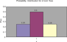
Example 12 Suppose, at each instant $s$ of the time interval $] 0, \tau]$, a share takes random value $x(s)$ (or $\left.x_{s}\right)$. Suppose $x(0)=x_{0}=1$ (with probability 1), and suppose, at each time $s(0<s \leq \tau)$, the share price takes value $x(s)$, $0 \leq x(s) \leq 1$, with uniform probability on $[0,1]$. Suppose the value at time $s$ is independent of the value taken at any other time. Suppose an investor takes an initial shareholding $z(0)$, or $z_{0}$, of 1 share (so $\left.z_{0}=1\right)$, and suppose the shareholding or number of shares $z(s)$ varies randomly at $m$ fixed times $\tau_{k}$ between initial time 0 and terminal time $\tau$, $$ 0=\tau_{0}<\tau_{1}<\tau_{2}<\cdots<\tau_{m}=\tau ; \quad M:=\left{\tau_{1}, \tau_{2}, \ldots, \tau_{m}\right} . $$ Thus $] 0, \tau]$ can be a period of $m$ days, with shareholding changing randomly at the end of each day. Suppose the random value $z_{\tau_{k}}$ (or simply $z_{k}$ ) of shares at time $\tau_{k}$ is independent of the value $z_{k^{\prime}}$ at any other time $\tau_{k^{\prime}}$, and independent of the value $x(s)$ of the share at any times. To keep things uncomplicated suppose that, at any time $\tau_{k}$, the shareholding $z_{k}$ is 1 with probability $0.5$, and $z_{k}=0$ with probability 0.5. What is the expected payout at terminal time $t$ from this shareholding?
The intention is to apply a stochastic integral calculation. But the probability distributions are deliberately chosen so that the expected payout is fairly obvious on intuitive grounds. Then it can be seen whether the stochastic integral calculation confirms what common sense indicates.
物理代写|电动力学代写electromagnetism代考|Stochastic Integrals for Example 12
Example 12 above has two independent stochastic processes, $$ Z_{\mathrm{T}} \simeq z_{\mathrm{T}}\left[\mathbf{R}^{\mathbf{T}}, F_{Z_{\mathrm{T}}}\right], \quad X_{\mathrm{T}} \simeq x_{\mathbf{T}}\left[\mathbf{R}^{\mathrm{T}}, F_{X_{\mathrm{T}}}\right] $$ with joint process $\left(Z_{\mathbf{T}}, X_{\mathrm{T}}\right)$ expressed by $$ \left(Z_{\mathbf{T}}, X_{\mathrm{T}}\right) \simeq\left(z_{\mathrm{T}}, x_{\mathrm{T}}\right)\left[(\mathbf{R} \times \mathbf{R})^{\mathbf{T}}, F_{\left(Z_{\mathrm{T}}, X_{\mathrm{T}}\right)}\right] $$
where each sample path $z_{\mathrm{T}}=(z(s): 0<s \leq \tau)$ is constant for $\tau_{j-1} \leq s<\tau_{j}$, $(1 \leq j \leq m)$.
The calculation in $(4.10)$ enabled us to disregard the random variation in $x(s)$ for $\tau_{j-1}<s<\tau_{j},(1 \leq j \leq m)$, so the joint processes can be expressed as $$ \left(Z_{M}, X_{M}\right) \simeq\left(z_{M}, x_{M}\right)\left[(\mathbf{R} \times \mathbf{R})^{M}, F_{\left(Z_{M}, X_{M}\right)}\right] $$ and the latter formulation enabled us to perform a calculation for the expected gain in portfolio value (or shareholding value).
Stochastic integrals $\int_{0}^{\tau} \cdots$ on domain $\left.\left.\mathbf{T}=\right] 0, \tau\right]$ can be formulated from version (4.16). The objective is to express the gains (or losses) in portfolio value $w(t)(0<t \leq \tau)$ in terms of joint sample paths $(z(s), x(s))(0<s \leq \tau)$ of the joint process $\left(Z_{\mathbf{T}}, X_{\mathrm{T}}\right)$. $$ \begin{aligned} &w(t)=\sum_{0 \leq s<s^{\prime} \leq t} z(s)\left(x\left(s^{\prime}\right)-x(s)\right), \quad \text { or } \ &w(t)=\int_{0}^{t} z(s) d x(s), \quad(0<t \leq \tau) . \end{aligned} $$ Thus $w(t)$ depends on the joint outcomes $((z(s), x(s)): 0<s \leq t)$, or $w(t)=$ $h\left(z_{\mathbf{T}}, x_{\mathbf{T}}\right)$ where $\left.\left.\mathbf{T}=\right] 0, t\right]$ and $h$ is the deterministic function given by the Stieltjes integral $\int_{0}^{t} z(s) d x(s)$ – if and when the latter integrals exist. These integrals are sample path versions of a stochastic integral $\int_{0}^{t} Z(s) d X(s)$, and can be examined further, in terms of particular sample paths, in order to try to understand whether or not they exist, and what other kinds of issues can arise with them.
Before undertaking this task, the random variability in the outcomes $(w(t)$ : $0<t \leq \tau)$ can be examined. Write $U_{\mathbf{T}}$ for the joint processes $\left(Z_{\mathbf{T}}, X_{\mathrm{T}}\right)$, so a sample path for $U_{\mathbf{T}}$ is $u_{\mathbf{T}}=\left(z_{\mathbf{T}}, x_{\mathbf{T}}\right)$. Then (4.16) gives $$ W_{\mathbf{T}}=h\left(U_{\mathbf{T}}\right) \simeq h\left(u_{\mathbf{T}}\right)\left[(\mathbf{R} \times \mathbf{R})^{\mathbf{T}}, F_{U_{\mathbf{T}}}\right], $$ where $F_{U_{\mathbf{T}}}$ is the joint distribution function $F_{\left(Z_{\mathbf{T}}, X_{\mathrm{T}}\right)}$ mentioned in (4.16), and $h\left(U_{\mathbf{T}}\right)$ is the stochastic integral $\int_{0}^{t} Z(s) d X(s)$. Thus $W_{\mathbf{T}}$ is a contingent process depending on the joint values of the processes $Z_{\mathrm{T}}, X_{\mathrm{T}}$.
The details of $F_{\left(Z_{M}, X_{M}\right)}$ were described above, but not those of $F_{\left(Z_{T}, X_{\mathrm{T}}\right)}$. These are provided in Section $4.4$ below.
Example 13 demonstrates that stochastic integrals can fail to exist even in the relatively simple case of Example 12. It has been pointed out that (4.15) delivers $\mathrm{E}[W(\tau)]$ without constructing stochastic integrals. The joint distribution function used in that calculation is $F_{U_{M}},=F_{\left(Z_{M}, X_{M}\right)}$ as in (4.17).
Compare this with (4.8), where the sample space for the elementary form of the random variable $W(\tau)$ is $\mathbf{R}$, with distribution function $F_{W_{\tau}}$. The difference between the elementary and joint basic representations of joint random variability was described in Section 3.5. In the elementary format (4.8), the expected value of $W(\tau)$ is obtained by integration on $\mathbf{R}$ with respect to $F_{W_{\tau}}$. Likewise for any contingent observable $f(W(\tau))$ that might arise.
In contrast, $(4.20)$ and $(4.16)$ employ $(\mathbf{R} \times \mathbf{R})^{\mathbf{T}}$ as sample space for $W_{\tau}$; and the joint distribution function is $F_{U_{T}},=F_{\left(Z_{T}, X_{T}\right)}$ (or $F_{Z_{T} X_{T}}$ ); but this distribution function was left unspecified. At this point it is useful to pursue this approach to $\mathrm{E}[W(\tau)]$ a bit further. Here is a summary of what is involved:
With $W(\tau) \simeq w(\tau)\left[\mathbf{R}, F_{W(\tau)}\right]$, expected gain in portfolio value at time $\tau$ can be calculated as $$ \mathrm{E}[W(\tau)]=\int_{\mathbf{R}} w(\tau) F_{W(\tau)}\left(I_{\tau}\right) $$
With $W(\tau)=f\left(X_{M}, Z_{M}\right) \simeq f\left(x_{M}, z_{M}\right)\left[(\mathbf{R} \times \mathbf{R})^{M}, F_{X_{M} Z_{M}}\right]$, expected gain in portfolio value at time $\tau$ can be calculated as $$ \begin{aligned} \mathrm{E}[W(\tau)] &=\mathrm{E}\left[f\left(X_{M}, Z_{M}\right)\right] \ &=\int_{(\mathbf{R} \times \mathbf{R})^{M}} f\left(x_{M}, z_{M}\right) F_{X_{M} Z_{M}}\left(I_{X_{M}}(M) \times I_{Z_{M}}(M)\right) \end{aligned} $$ Interval notation $I_{X_{M}}, I_{Z_{M}}$, refers to events (or sets of potential occurrences) of random variables $X_{M}, Z_{M}$, respectively.
Unlike algebra or calculus for instance, historians of the theory of probability often claim that, while it has a pre-history in gambling practice, this subject is a relative newcomer in mathematical terms.
Ideas of random variability and probability were put on a firmer mathematical basis in the course of the nineteenth century, and the modern form of the theory was well established by the mid-twentieth century.
An elementary link between statistics and probability is demonstrated in Sections $2.1$ and $2.2$ above, and the Riemann sum calculations of Example 4 indicate the central role of mathematical integration in analysis of random variation.
Twentieth century developments in probability and random variation are closely linked to developments in the theory of measure and integration culminating in Lebesgue’s theory of the integral [100]. A.N. Kolmogorov [93] made this the foundation of probability theory by identifying-
the probability of an event as the measure of a set,
a random variable as a measurable function, and
the expected value of a random variable as the integral of a measurable function with respect to a probability measure.
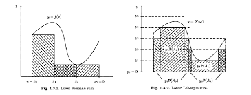
One of the standard ways of defining the Lebesgue integral of a $\mu$-measurable function $f(\omega)(\omega \in \Omega)$ is to form finite sums $$ s_{j}=\sum_{r=1}^{n} \phi_{j}^{(r)}(\omega) \mu\left(A_{j}^{(r)}\right) $$ of simple functions $\phi_{j}(\omega)$ which converge to $f$ as $j \rightarrow \infty$, and then define the Lebesgue integral of $f$ on $\Omega$ by $$ \int_{\Omega} f(\omega) d \mu=\lim {j \rightarrow \infty} s{j} . $$
The dominated convergence theorem emerges from this: Suppose Lebesgue integrable functions $f_{j}(\omega)$ converge almost everywhere to $f(\omega)$, with $\left|f_{j}(\omega)\right| \leq g(\omega)$ almost everywhere, $g$ also being Lebesgue integrable. Then $f$ is Lebesgue int egrable, and $\int_{\Omega} f_{j}$ converges to $\int_{\Omega} f$ as $j \rightarrow \infty$.
Depending on the measurable integrand $f$, the measurable sets $A_{j}^{(r)}$ in Definition $3.1$ can be intervals, open sets, closed sets, isolated points, and/or various countable combinations of these and other even more complicated sets. One could say that the means used to access the integral of $f$ are themselves somewhat arcane and inaccessible. The “cure” (finding appropriate measurable sets) could be worse than the “disease” (finding the integral). ${ }^{1}$
The entrance to measure theory and Lebesgue integration is guarded by such fearsome sets and functions as the Cantor set, and the Devil’s Staircase or Cantor function [102]. But while it is unwise to enter the house of Lebesgue without keeping an eye out for monsters ${ }^{2}$, in the simple examples of essentially finite domains of preceding chapters we managed to negotiate our way fairly painlessly through the relevant measurable sets/functions. (Would we be so lucky if the domains were infinite, or the functions a bit more complicated?) These monsters will never completely go away. But perhaps it would be better to not have to wrestle with them as a pre-condition of gaining entry to the house. It would be nice if the monsters were kept locked up in the cellar, not on guard at the front door. Is there any other way to deal with probability which provides full mathematical power and rigour? Is there another house, one that is more easily accessible, and closer to the “naive” or realistic view of random variability, as outlined in Chapter 2 above, and in [MTRV] pages $15-17 ?$
物理代写|电动力学代写electromagnetism代考|Burkill-complete Stochastic Integral
In contrast, the Burkill integral ([13], [14], [68]) involves integrator functions $h(I)$ which are not additive it is not required that $h(I)=h\left(I^{\prime}\right)+h\left(I^{\prime \prime}\right)$. (Of course, it is not forbidden either!)
It turns out that a version of the Burkill integral is very useful in a reformulated theory of stochastic integration, and in the Feynman integral theory of quantum mechanics. In [MTRV], in addition to dependence on cells $I$, an extended Burkill integrand $h(s, I)$ is allowed to depend also on tag points $s$ of cells $I$; and from this is developed a Burkill-complete form of integration. (A Burkill-complete integrand $h$ is not additive in respect of its dependence on cells $I$ – if it is additive it receives a different designation.)
Definition 6 below fits into the -complete structure of definitions. It deals with integrands $h(s, I)$ which are functions of tagged intervals $(\bar{s}, I)$ (or associated point-interval pairs $(\bar{s}, I))$; for instance, with $\left.I=] s^{\prime}, s^{\prime \prime}\right], \bar{s}=s^{\prime}$ or $s^{\prime \prime}$, $$ h(s, I)=\sqrt{\bar{s}\left(s^{\prime \prime}-s^{\prime}\right)} $$ and a partition $\mathcal{P}=\left{0=s_{0}, s_{1}, \ldots, s_{n-1}, s_{n}=1\right}$ of $\left.] 0,1\right]$ is a finite sample of points of the domain. Then $h(s, I)=\sqrt{\bar{s}{j}\left(s{j}-s_{j-1}\right)}$ with $\bar{s}{j}=s{j}$ or $s_{j-1}$; and a Riemann sum $(\mathcal{P}) \sum h(s, I)$ is a functional of samples of points: $$ (\mathcal{P}) \sum h(x, I)=\sum_{j=1}^{n} \sqrt{\bar{s}{j}\left(s{j}-s_{j-1}\right)} $$ This formulation changes the perspective of -complete integration from pointcell pairs to finite samples of points. Nevertheless, as in chapter 4 of [MTRV], the underlying structures can be readily conveyed in terms of relationships between cells or intervals $I$ of the domain.
In effect, adjacent pairs of points $\left(s_{j}, s_{j-1}\right)$ from the finite sample $\mathcal{P}$ must satisfy conditions corresponding to Axioms DS1 to DS8 in chapter 4 (pages 111-113 of [MTRV]). Of course, in simple domains such as $] 0,1]$ it is natural to visualize pairs of points $\left(s_{j}, s_{j-1}\right)$ as intervals $I_{j}$. But in the more complicated and structured domains used in quantum field theory (Chapters 8 and 9 below), the alternative “samples of points” perspective may be helpful.
Lebesgue integration uses functions $\mu(A)$ of measurable subsets of a domain. In contrast, -complete integration uses functions $\mu(I)$ of subintervals of the domain. The latter can be replaced by $\mu\left(s^{\prime}, s^{\prime \prime}\right)$ (where $\left.\left.I=\right] s^{\prime}, s^{\prime \prime}\right]$ ). But measurable sets $A$ can consist of infinitely many intervals and discrete points, ruling out the “finite sample of points” approach.
物理代写|电动力学代写electromagnetism代考|The Henstock Integral
The origins of the ideas in chapter 4 of [MTRV] are as follows. Starting with his $1948 \mathrm{PhD}$ thesis, Ralph Henstock (1923-2007) worked in non-absolute integration, including the Riemann-complete or gauge integral which, independently, Jaroslav Kurzweil also discovered in the 1950 s. As a Cambridge undergraduate (1941-1943) Henstock took a course of lectures, given by J.C. Burkill, on the integration of non-additive interval functions. Later, under the supervision of Paul Dienes in Birkbeck College, London, he undertook research into the ideas of Burkill (interval function integrands) and of Dienes (Stieltjes integrands); and he presented this thesis in December $1948 .$
In terms of overall approach and methods of proof, the thesis contains the germ of Henstock’s later work as summarized in chapter 4 of [MTRV]. For example, a notable innovation is a set of axioms for constructing any particular system of integration. This approach highlights the features held in common by various systems, so that a particular property or theorem can, by a single, common proof, be shown to hold for various kinds of integration. These ideas are the basis of the theory in chapter 4 of [MTRV].
Within this approach, Henstock’s thesis places particular emphasis on various alternative ways of selecting Riemann sums, as constituting the primary distinguishing feature of different systems of integration. This was central to his subsequent work and achievement. Accordingly, the theory in chapter 4 of [MTRV] is designated there as the Henstock integral, from which almost all systems of integration can be deduced.
Robert Bartle’s book ([5], page 15) has a discussion of titles for this kind of
integral-variously called Kurzweil-Henstock, gauge, or generalized Riemann. Bartle suggests that it could equally be called “the Denjoy-Perron-KurzweilHenstock integral”. Evading this litany, Bartle settles for “generalized Riemann”, or simply “the integral”.
The first worked-out version of this kind of integration was in Henstock’s Theory of Integration [70], published in 1962 and re-published in 1963 , in which the integral was designated “Riemann-complete”. In support of the “-complete” appendage, Henstock’s presentation has theorems which justify the integration of limits of integrable functions, differentiation under the integral sign, Fubini’s theorem, along with a theory of variation corresponding to measure theory.
物理代写|电动力学代写electromagnetism代考|A Basic Stochastic Integral
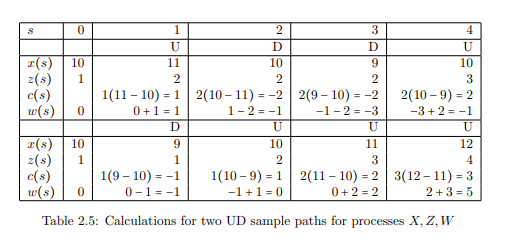
The following is similar to Example $2 .$ Example 5 Suppose $s=1,2,3, \ldots$ is time, measured in days. Suppose a share, or unit of stock, has value $x(s)$ on day s; suppose $z(s)$ is the number of shares held on day $s$; and suppose $c(s)$ is the change in the value of the shareholding on day $s$ as a result of the change in share value from the previous day so $c(s)=$ $z(s-1)(x(s)-x(s-1))$. Let $w(s)$ be the cumulative change in shareholding value at end of day $s$, so $w(s)=w(s-1)+c(s)$. If share value $x(s)$ and stockholding $z(s)$ are subject to random variability, how is the gain (or loss) from the stockholding to be estimated?
Take initial value (at time $s=0)$ of the share to be $x(0)$ (or $\left.x_{0}\right)$, take the initial shareholding or number of shares owned to be $z(0)$ (or $\left.z_{0}\right)$. Then, at end of day $1(s=1)$, $$ c(1)=z(0) \times(x(1)-x(0)), \quad w(1)=w(0)+c(1)=c(1) $$ At end of day $s$, $$ c(s)=z(s-1) \times(x(s)-x(s-1)), \quad w(s)=w(s-1)+c(s) $$ After $t$ days, $$ w(t)=\sum_{s=1}^{t} z(s-1)(x(s)-x(s-1)) . $$ If the time increments are reduced to arbitrarily small size (so $s$ represents number of “time ticks” -fractions of a second, say), with the meaning of the other variables adjusted accordingly, then $$ w(t)=\sum_{j=1}^{n} z\left(s_{j-1}\right)\left(x\left(s_{j}\right)-x\left(s_{j-1}\right)\right), \quad \text { or } \quad w(t)=\sum z(s) \Delta x(s) $$ The latter expressions are Riemann sum estimates of $\int_{0}^{t} z(s) d x(s)$ (a Stieltjestype integral) whenever the latter exists. Each of the expressions in (2.4) is sample value of a random variable $$ W(t)=\sum_{j=1}^{n} Z\left(s_{j-1}\right)\left(X\left(s_{j}\right)-X\left(s_{j-1}\right)\right) \text { or } \int_{0}^{t} Z(s) d X(s) $$constructed from the random variables $X, Z$, and $W$. These notations symbolize in a “naive” or “realistic” way-the stochastic integral of the process $Z$ with respect to the process $X$. In chapter 8 of [MTRV], symbols s, or $\mathbf{S}$, or $\mathcal{S}$ are used (in place of the symbol $\int$ ) for various kinds of stochastic integral. In the context described here, S would be the appropriate notation. (See (5.28) below.)
物理代写|电动力学代写electromagnetism代考|Choosing a Sample Space
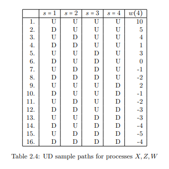
It was mentioned earlier that there are many alternative ways of producing a sample space $\Omega$ (along with the linked probability measure $P$ and family $\mathcal{A}$ of measurable subsets of $\Omega$ ). The set of numbers $$ {-5,-4,-3,-2,-1,0,1,2,3,4,5,10} $$ was used as sample space for the random variability in the preceding example of stochastic integration. The measurable space $\mathcal{A}$ was the family of all subsets of $\Omega$, and the example was illustrated by means of two distinct probability measures $P$, one of which was based on Up and Down transitions being equally likely, where for the other measure an Up transition was twice as likely as a Down. An alternative sample space for this example of random variability is $$ \Omega=\Omega \Omega_{1} \times \Omega \Omega_{2} \times \Omega \Omega_{3} \times \Omega \Omega_{4} $$ where $\Omega_{j}={U, D}$ for $j=1,2,3,4$; so the elements $\omega$ of $\Omega$ consist of sixteen 4-tuples of the form $$ \omega=(\cdot, \cdot \cdot \cdot), \quad \text { such as } \omega=(U, D, D, U) \text { for example. } $$ Let the measurable space $\mathcal{A}$ be the family of all subsets $A$ of $\Omega$; so $\mathcal{A}$ contains $2^{16}$ members, one of which (for example) is $$ A={(D, U, U, D),(U, D, D, U),(D, U, D, U),(U, U, U, U),(D, D, D, D)} $$
with $A$ consisting of five individual four-tuples. Assume that Up transitions and Down transitions are equally likely, and that they are independent events. Then, as before, $$ P({\omega})=\frac{1}{16} $$ for each $\omega \in \Omega$. For $A$ above, $P(A)=\frac{5}{16}$. To relate this probability structure to the shareholding example, let $\mathbf{R}^{4}=$ $\mathbf{R} \times \mathbf{R} \times \mathbf{R} \times \mathbf{R}$, and let $$ f: \Omega \mapsto \mathbf{R}^{4}, \quad f(\omega)=((x(1), x(2), x(3), x(4)), $$ using Table 2.4; so, for instance, $$ f(\omega)=f((U, D, D, U))=(11,10,9,10)=(x(1), x(2), x(3), x(4)), $$ and so on. Next, let $\mathbf{S}$ denote the stochastic integrals of the preceding section, so for $x=(x(1), x(2), x(3), x(4)) \in \mathbf{R}^{4}$, $$ \mathbf{S}(x)=\int_{0}^{4} z(s) d x(s)=\sum_{s=1}^{4} z(s-1)(x(s)-x(s-1)), $$ so $\mathbf{S}(x)$ gives the values $w(4)$ of Table 2.4. As described in Section $2.3$, the rationale for deducing the probabilities of outcomes $\mathbf{S}(x)$, = $w(4)$, from the probabilities on $\Omega$ is the relationship $$ P(w(4))=P\left(f^{-1}\left(\mathbf{S}^{-1}(w(4))\right)\right) . $$
物理代写|电动力学代写electromagnetism代考|More on Basic Stochastic Integral
The constructions in Sections $2.3$ and $2.4$ purported to be about stochastic integration. While a case can be made that (2.6) and (2.7) are actually stochastic integrals, such simple examples are not really what the standard or classical theory of Chapter 1 is all about. The examples and illustrations in Sections $2.3$ and $2.4$ may not really be much help in coming to grips with the standard theory of stochastic integrals outlined in Chapter $1 .$
This is because Chapter 1, on the definition and meaning of classical stochastic integration, involves subtle passages to a limit, whereas (2.6) and (2.7) involve only finite sums and some elementary probability calculations.
From the latter point of view, introducing probability measure spaces and random-variables-as-measurable-functions seems to be an unnecessary complication. So, from such a straightforward starting point, why does the theory become so challenging and “messy”, as portrayed in Chapter $1 ?$
As in Example 2, the illustration in Section $2.3$ involves dividing up the time period (4 days) into 4 sections; leading to sample space $\Omega=\mathbf{R}^{4}$ in (2.15). Why not simply continue in this vein, and subdivide the time into 40 , or 400 , or 4 million steps instead of just 4 ; using sample spaces $\mathbf{R}^{40}$, or $\mathbf{R}^{400}$, or $\mathbf{R}^{4000000}$, respectively? The computations may become lengthier, but no new principle is involved; each of the variables changes in discrete steps at discrete points in time. ${ }^{5}$
Other simplifications can be similarly adopted. For instance, only two kinds of changes are contemplated in Section 2.3: increase (Up) or decrease (Down).