STAT 7430 - 统计代写答疑辅导

标签： STAT 7430

统计代写|Generalized linear model代考广义线性模型代写|Probability and the Central Limit Theorem

Posted on 2022年5月18日2022年5月18日 by statistics-lab

如果你也在怎样代写Generalized linear model这个学科遇到相关的难题，请随时右上角联系我们的24/7代写客服。

广义线性模型（GLiM，或GLM）是John Nelder和Robert Wedderburn在1972年提出的一种高级统计建模技术。它是一个包括许多其他模型的总称，它允许响应变量y具有正态分布以外的误差分布。

statistics-lab™ 为您的留学生涯保驾护航在代写Generalized linear model方面已经树立了自己的口碑, 保证靠谱, 高质且原创的统计Statistics代写服务。我们的专家在代写Generalized linear model代写方面经验极为丰富，各种代写Generalized linear model相关的作业也就用不着说。

我们提供的Generalized linear model及其相关学科的代写，服务范围广, 其中包括但不限于:

Statistical Inference 统计推断
Statistical Computing 统计计算
Advanced Probability Theory 高等概率论
Advanced Mathematical Statistics 高等数理统计学
(Generalized) Linear Models 广义线性模型
Statistical Machine Learning 统计机器学习
Longitudinal Data Analysis 纵向数据分析
Foundations of Data Science 数据科学基础

统计代写|Generalized linear model代考广义线性模型代写|Probability and the Central Limit Theorem

统计代写|Generalized linear model代考广义线性模型代写|Basic Probability

Statistics is based entirely on a branch of mathematics called probability, which is concerned with the likelihood of outcomes for an event. In probability theory, mathematicians use information about

all possible outcomes for an event in order to determine the likelihood of any given outcome. The first section of this chapter will explain the basics of probability before advancing to the foundational issues of the rest of the textbook.

Imagine an event repeated 100 times. Each of these repetitions – called a trial – would be recorded. Mathematically, the formula for probability (abbreviated $p$ ) is:
$$
p=\frac{\text { Number of trials with the same outcome }}{\text { Total number of trials }}
$$
(Formula 6.1)
To calculate the probability of any given outcome, it is necessary to count the number of trials that resulted in that particular outcome and divide it by the total number of trials. Thus, if the 100 trials consisted of coin flips – which have two outcomes, heads and tails – and 50 trials resulted in “heads” and 50 trials resulted in “tails,” the probability of the coin landing heads side up would then be $\frac{50}{100}$ ” To simplify this notation, it is standard to reduce the fraction to its simplest form or to convert it to a decimal: $1 / 2$ or $.50$ in this example.

This is called the empirical probability because it is based on empirical data collected from actual trials. Some readers will notice that this is the same method and formula for calculating the relative frequency in a frequency table (see Chapter 3). Therefore, empirical probabilities have the same mathematical properties as relative frequencies. That is, probability values always range from 0 to 1 . A probability of zero indicates that the outcome never occurred, and a probability value of 1 indicates that the outcome occurred for every trial (and that no other outcome occurred). Also, all probabilities for a trial must add up to 1 – just as all relative frequencies in a dataset must add up to 1 .

Interpreting probability statistics only requires an understanding of percentages, fractions, and decimals. In the coin-flipping example, a probability of $.50$ indicates that we can expect that half of those trials would result in an outcome of “heads.” Similarly, the chances that any particular trial will result in an outcome of “heads” is $50 \%$. Mathematically, it really doesn’t matter whether probability values are expressed as percentages (e.g., $50 \%$ ), fractions (e.g., 1/2), or decimals (e.g., .50). Statisticians, though, prefer to express probabilities as decimals, and this textbook will stick to that convention.

统计代写|Generalized linear model代考广义线性模型代写|The Logic of Inferential Statistics and the CLT

The beginning of this book, especially Chapter 4, discussed descriptive statistics, which is the branch of statistics concerned with describing data that have been collected. Descriptive statistics are indispensable for understanding data, but they are often of limited usefulness because most social scientists wish to make conclusions about the entire population of interest – not just the subjects in the sample that provided data to the researcher. For example, in a study of bipolar mood disorders, Kupka et al. (2007) collected data from 507 patients to examine how frequently they were in manic, hypomanic, and depressed mood states. The descriptive statistics that Kupka et al. provided are interesting – but they are of limited use if they only apply to the 507 people in the study. The authors of this study – and the vast majority of researchers – want to apply their conclusions to the entire population of people they are studying, even people who are not in the sample. The process of drawing conclusions about the entire population based on data from a sample is called generalization, and it requires inferential statistics in order to be possible. Inferential statistics is the branch of statistics that builds on the foundation of probability in order to make generalizations.
The logic of inferential statistics is diagrammed in Figure 6.6. It starts with a population, which, for a continuous, interval- or ratio-level variable, has an unknown mean and unknown standard deviation (represented as the circle in the top left of Figure 6.6). A researcher then draws a random sample from the population and uses the techniques discussed in previous chapters to calculate a sample mean and create a sample histogram. The problem with using a single sample to learn about the population is that there is no way of knowing whether that sample is typical – or representative – of the population from which it is drawn. It is possible (although not likely if the

sampling method was truly random) that the sample consists of several outliers that distort the sample mean and standard deviation.

The solution to this conundrum is to take multiple random samples with the same $n$ from the population. Because of natural random variation in which population members are selected for a sample, we expect some slight variation in mean values from sample to sample. This natural variation across samples is called sampling error. With several samples that all have the same sample size, it becomes easier to judge whether any particular sample is typical or unusual because we can see which samples differ from the others (and therefore probably have more sampling error). However, this still does not tell the researcher anything about the population. Further steps are needed to make inferences about the population from sample data.

After finding a mean for each sample, it is necessary to create a separate histogram (in the middle of Figure 6.6) that consists solely of sample means. The histogram of means from a series of samples is called a sampling distribution of means. Sampling distributions can be created from

other sample statistics (e.g., standard deviations, medians, ranges), but for the purposes of this chapter it is only necessary to talk about a sampling distribution of means.

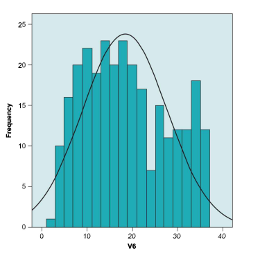
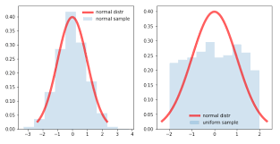
Because a sampling distribution of means is produced by a purely random process, its properties are governed by the same principles of probability that govern other random outcomes, such as dice throws and coin tosses. Therefore, there are some regular predictions that can be made about the properties of the sampling distribution as the number of contributing samples increases. First, with a large sample size within each sample, the shape of the sampling distribution of means is a normal distribution. Given the convergence to a normal distribution, as shown in Figures 6.4a-6.4d, this should not be surprising. What is surprising to some people is that this convergence towards a normal distribution occurs regardless of the shape of the population, as long as the $\mathrm{n}$ for each sample is at least 25 and all samples have the same sample size. This is the main principle of the CLT.

统计代写|Generalized linear model代考广义线性模型代写|Summary

The basics of probability form the foundation of inferential statistics. Probability is the branch of mathematics concerned with estimating the likelihood of outcomes of trials. There are two types of probabilities that can be estimated. The first is the empirical probability, which is calculated by conducting a large number of trials and finding the proportion of trials that resulted in each outcome, using Formula 6.1. The second type of probability is the theoretical probability, which is calculated by dividing the number of methods of obtaining an outcome by the total number of possible outcomes. Adding together the probabilities of two different events will produce the probability that either one will occur. Multiplying the probabilities of two events together will produce the joint probability, which is the likelihood that the two events will occur at the same time or in succession.
With a small or moderate number of trials, there may be discrepancies between the empirical and theoretical probabilities. However, as the number of trials increases, the empirical probability converges to the value of the theoretical probability. Additionally, it is possible to build a histogram of outcomes of trials from multiple events; dividing the number of trials that resulted in each outcome by the total number of trials produces an empirical probability distribution. As the number of trials increases, this empirical probability distribution gradually converges to the theoretical probability distribution, which is a histogram of the theoretical probabilities.

If an outcome is produced by adding together the results of multiple independent events, the theoretical probability distribution will be normally distributed. Additionally, with a large number of trials, the empirical probability distribution will also be normally distributed. This is a result of the CLT.

The CLT states that a sampling distribution of means will be normally distributed if the size of each sample is at least 25. As a result of the CLT, it is possible to make inferences about the population based on sample data – a process called generalization. Additionally, the mean of the sample means converges to the population mean as the number of samples in a sampling distribution increases. Likewise, the standard deviation of means in the sampling distribution (called the standard error) converges on the value of $\frac{\sigma}{\sqrt{n}}$.

广义线性模型代写

统计代写|Generalized linear model代考广义线性模型代写|Basic Probability

统计学完全基于称为概率的数学分支，它与事件结果的可能性有关。在概率论中，数学家使用关于

事件的所有可能结果，以确定任何给定结果的可能性。本章的第一部分将解释概率的基础知识，然后再讨论教科书其余部分的基础问题。

想象一个事件重复了 100 次。这些重复中的每一个——称为试验——都会被记录下来。在数学上，概率公式（缩写为p）是：
p= 相同结果的试验次数试验总数
（公式 6.1）
为了计算任何给定结果的概率，有必要计算导致该特定结果的试验次数并将其除以试验总数。因此，如果 100 次试验包括抛硬币——有两种结果，正面和反面——并且 50 次试验产生“正面”，50 次试验产生“反面”，那么硬币正面朝上的概率为50100” 为了简化这个符号，将分数简化为最简单的形式或将其转换为小数是标准的：1/2或者.50在这个例子中。

这被称为经验概率，因为它基于从实际试验中收集的经验数据。有些读者会注意到，这与计算频率表中相对频率的方法和公式相同（参见第 3 章）。因此，经验概率与相对频率具有相同的数学性质。也就是说，概率值的范围总是从 0 到 1 。概率为零表示结果从未发生，概率值为 1 表示每次试验都发生了结果（并且没有发生其他结果）。此外，试验的所有概率加起来必须为 1 – 就像数据集中的所有相对频率加起来必须为 1 一样。

解释概率统计只需要了解百分比、分数和小数。在掷硬币的例子中，概率为.50表明我们可以预期其中一半的试验会产生“正面”的结果。同样，任何特定试验导致“正面”结果的可能性是50%. 在数学上，概率值是否表示为百分比实际上并不重要（例如，50%)、分数（例如，1/2）或小数（例如，0.50）。不过，统计学家更喜欢将概率表示为小数，而这本教科书将坚持这一惯例。

统计代写|Generalized linear model代考广义线性模型代写|The Logic of Inferential Statistics and the CLT

本书的开头，尤其是第 4 章，讨论了描述性统计，这是与描述已收集数据有关的统计分支。描述性统计对于理解数据是必不可少的，但它们的用处通常有限，因为大多数社会科学家希望对整个感兴趣的人群做出结论——而不仅仅是样本中向研究人员提供数据的受试者。例如，在双相情绪障碍的研究中，Kupka 等人。(2007) 收集了 507 名患者的数据，以检查他们处于躁狂、轻躁狂和抑郁情绪状态的频率。Kupka 等人的描述性统计数据。提供的内容很有趣——但如果它们仅适用于研究中的 507 人，则它们的用途有限。这项研究的作者——以及绝大多数研究人员——希望将他们的结论应用于他们正在研究的整个人群，甚至是不在样本中的人。根据样本数据得出关于整个人口的结论的过程称为泛化，它需要推论统计才能成为可能。推论统计是统计的一个分支，它建立在概率的基础上以进行概括。
推论统计的逻辑如图 6.6 所示。它从一个总体开始，对于一个连续的、区间或比率水平的变量，该总体具有未知的平均值和未知的标准差（表示为图 6.6 左上角的圆圈）。然后，研究人员从总体中抽取一个随机样本，并使用前面章节中讨论的技术来计算样本均值并创建样本直方图。使用单个样本来了解总体的问题在于，无法知道该样本是否是其所来自的总体的典型（或代表性）。这是可能的（虽然不太可能，如果

抽样方法是真正随机的）样本由几个异常值组成，这些异常值扭曲了样本均值和标准偏差。

解决这个难题的方法是随机抽取多个相同的样本n从人口。由于为样本选择人口成员的自然随机变化，我们预计样本之间的平均值会略有变化。这种跨样本的自然变化称为抽样误差。对于具有相同样本量的多个样本，判断任何特定样本是典型的还是异常的变得更容易，因为我们可以看到哪些样本与其他样本不同（因此可能有更多的抽样误差）。然而，这仍然没有告诉研究人员有关人口的任何信息。需要进一步的步骤来从样本数据中推断出总体。

在找到每个样本的均值后，有必要创建一个单独的直方图（在图 6.6 的中间），它仅由样本均值组成。来自一系列样本的均值直方图称为均值的抽样分布。抽样分布可以从

其他样本统计数据（例如，标准差、中位数、范围），但为了本章的目的，只需要讨论均值的抽样分布。

因为均值的抽样分布是由纯随机过程产生的，所以它的属性受支配其他随机结果（例如掷骰子和掷硬币）的相同概率原则支配。因此，随着贡献样本数量的增加，可以对采样分布的属性进行一些常规预测。首先，每个样本内的样本量很大，均值的抽样分布的形状是正态分布。鉴于收敛到正态分布，如图 6.4a-6.4d 所示，这应该不足为奇。令一些人惊讶的是，无论人口的形状如何，这种趋向正态分布的收敛都会发生，只要n每个样本至少有 25 个，并且所有样本都具有相同的样本量。这是 CLT 的主要原则。

统计代写|Generalized linear model代考广义线性模型代写|Summary

概率的基础构成了推理统计的基础。概率是与估计试验结果的可能性有关的数学分支。有两种类型的概率可以估计。第一个是经验概率，它是通过进行大量试验并使用公式 6.1 找到导致每个结果的试验比例来计算的。第二种概率是理论概率，它是通过将获得结果的方法数除以可能结果的总数来计算的。将两个不同事件的概率相加将产生其中任何一个事件发生的概率。将两个事件的概率相乘将产生联合概率，
对于少量或中等数量的试验，经验概率和理论概率之间可能存在差异。然而，随着试验次数的增加，经验概率会收敛到理论概率的值。此外，可以从多个事件中构建试验结果的直方图；将导致每个结果的试验次数除以试验总数产生经验概率分布。随着试验次数的增加，这种经验概率分布逐渐收敛到理论概率分布，即理论概率的直方图。

如果一个结果是通过将多个独立事件的结果相加而产生的，那么理论上的概率分布将是正态分布的。此外，随着大量试验，经验概率分布也将呈正态分布。这是 CLT 的结果。

CLT 指出，如果每个样本的大小至少为 25，则均值的抽样分布将呈正态分布。由于 CLT，可以根据样本数据对总体进行推断——这一过程称为泛化。此外，随着抽样分布中样本数量的增加，样本均值的均值会收敛到总体均值。同样，抽样分布中均值的标准差（称为标准误差）收敛于σn.

统计代写|Generalized linear model代考广义线性模型代写请认准statistics-lab™

统计代写请认准statistics-lab™. statistics-lab™为您的留学生涯保驾护航。

金融工程代写

金融工程是使用数学技术来解决金融问题。金融工程使用计算机科学、统计学、经济学和应用数学领域的工具和知识来解决当前的金融问题，以及设计新的和创新的金融产品。

非参数统计代写

非参数统计指的是一种统计方法，其中不假设数据来自于由少数参数决定的规定模型；这种模型的例子包括正态分布模型和线性回归模型。

广义线性模型代考

广义线性模型（GLM）归属统计学领域，是一种应用灵活的线性回归模型。该模型允许因变量的偏差分布有除了正态分布之外的其它分布。

术语广义线性模型（GLM）通常是指给定连续和/或分类预测因素的连续响应变量的常规线性回归模型。它包括多元线性回归，以及方差分析和方差分析（仅含固定效应）。

有限元方法代写

有限元方法（FEM）是一种流行的方法，用于数值解决工程和数学建模中出现的微分方程。典型的问题领域包括结构分析、传热、流体流动、质量运输和电磁势等传统领域。

有限元是一种通用的数值方法，用于解决两个或三个空间变量的偏微分方程（即一些边界值问题）。为了解决一个问题，有限元将一个大系统细分为更小、更简单的部分，称为有限元。这是通过在空间维度上的特定空间离散化来实现的，它是通过构建对象的网格来实现的：用于求解的数值域，它有有限数量的点。边界值问题的有限元方法表述最终导致一个代数方程组。该方法在域上对未知函数进行逼近。[1] 然后将模拟这些有限元的简单方程组合成一个更大的方程系统，以模拟整个问题。然后，有限元通过变化微积分使相关的误差函数最小化来逼近一个解决方案。

tatistics-lab作为专业的留学生服务机构，多年来已为美国、英国、加拿大、澳洲等留学热门地的学生提供专业的学术服务，包括但不限于Essay代写，Assignment代写，Dissertation代写，Report代写，小组作业代写，Proposal代写，Paper代写，Presentation代写，计算机作业代写，论文修改和润色，网课代做，exam代考等等。写作范围涵盖高中，本科，研究生等海外留学全阶段，辐射金融，经济学，会计学，审计学，管理学等全球99%专业科目。写作团队既有专业英语母语作者，也有海外名校硕博留学生，每位写作老师都拥有过硬的语言能力，专业的学科背景和学术写作经验。我们承诺100%原创，100%专业，100%准时，100%满意。

随机分析代写

随机微积分是数学的一个分支，对随机过程进行操作。它允许为随机过程的积分定义一个关于随机过程的一致的积分理论。这个领域是由日本数学家伊藤清在第二次世界大战期间创建并开始的。

时间序列分析代写

随机过程，是依赖于参数的一组随机变量的全体，参数通常是时间。随机变量是随机现象的数量表现，其时间序列是一组按照时间发生先后顺序进行排列的数据点序列。通常一组时间序列的时间间隔为一恒定值（如1秒，5分钟，12小时，7天，1年），因此时间序列可以作为离散时间数据进行分析处理。研究时间序列数据的意义在于现实中，往往需要研究某个事物其随时间发展变化的规律。这就需要通过研究该事物过去发展的历史记录，以得到其自身发展的规律。

回归分析代写

多元回归分析渐进（Multiple Regression Analysis Asymptotics）属于计量经济学领域，主要是一种数学上的统计分析方法，可以分析复杂情况下各影响因素的数学关系，在自然科学、社会和经济学等多个领域内应用广泛。

MATLAB代写

MATLAB 是一种用于技术计算的高性能语言。它将计算、可视化和编程集成在一个易于使用的环境中，其中问题和解决方案以熟悉的数学符号表示。典型用途包括：数学和计算算法开发建模、仿真和原型制作数据分析、探索和可视化科学和工程图形应用程序开发，包括图形用户界面构建MATLAB 是一个交互式系统，其基本数据元素是一个不需要维度的数组。这使您可以解决许多技术计算问题，尤其是那些具有矩阵和向量公式的问题，而只需用 C 或 Fortran 等标量非交互式语言编写程序所需的时间的一小部分。MATLAB 名称代表矩阵实验室。MATLAB 最初的编写目的是提供对由 LINPACK 和 EISPACK 项目开发的矩阵软件的轻松访问，这两个项目共同代表了矩阵计算软件的最新技术。MATLAB 经过多年的发展，得到了许多用户的投入。在大学环境中，它是数学、工程和科学入门和高级课程的标准教学工具。在工业领域，MATLAB 是高效研究、开发和分析的首选工具。MATLAB 具有一系列称为工具箱的特定于应用程序的解决方案。对于大多数 MATLAB 用户来说非常重要，工具箱允许您学习和应用专业技术。工具箱是 MATLAB 函数（M 文件）的综合集合，可扩展 MATLAB 环境以解决特定类别的问题。可用工具箱的领域包括信号处理、控制系统、神经网络、模糊逻辑、小波、仿真等。

R语言代写	问卷设计与分析代写
PYTHON代写	回归分析与线性模型代写
MATLAB代写	方差分析与试验设计代写
STATA代写	机器学习/统计学习代写
SPSS代写	计量经济学代写
EVIEWS代写	时间序列分析代写
EXCEL代写	深度学习代写
SQL代写	各种数据建模与可视化代写

统计代写|Generalized linear model代考广义线性模型代写|Linear Transformations and $z-S c o r e s$

Posted on 2022年5月18日2022年5月18日 by statistics-lab

如果你也在怎样代写Generalized linear model这个学科遇到相关的难题，请随时右上角联系我们的24/7代写客服。

我们提供的Generalized linear model及其相关学科的代写，服务范围广, 其中包括但不限于:

Statistical Inference 统计推断
Statistical Computing 统计计算
Advanced Probability Theory 高等概率论
Advanced Mathematical Statistics 高等数理统计学
(Generalized) Linear Models 广义线性模型
Statistical Machine Learning 统计机器学习
Longitudinal Data Analysis 纵向数据分析
Foundations of Data Science 数据科学基础

统计代写|Generalized linear model代考广义线性模型代写|Linear Transformations

To perform a linear transformation, you need to take a dataset and either add, subtract, multiply, or divide every score by the same constant. (You may remember from Chapter 1 that a constant is a score that is the same for every member of a sample or population.) Performing a linear transformation is common in statistics. Linear transformations change the data, and that means they can have an impact on models derived from the data – including visual models and descriptive statistics.

Linear transformations allow us to convert data from one scale to a more preferable scale. For example, converting measurements recorded in inches into centimeters requires a linear transformation (multiplying by 2.54). Another common linear transformation is to convert Fahrenheit temperatures to Celsius temperatures (which requires subtracting 32 and then dividing by 1.8) or vice versa (which requires multiplying by $1.8$ and then adding 32 ). Sometimes performing a linear transformation is done to make calculations easier, as by eliminating negative numbers (by adding a constant so that all scores are positive) or eliminating decimals or fractions (by multiplying by a constant). As you will see in this chapter, making these changes in the scale of the data does not fundamentally alter the relative pattern of the scores or the results of many statistical analyses.

Linear transformations are common in statistics, so it is important to understand how linear transformations change statistics and data.

Impact of linear transformations on means. Chapter 4 showed how to calculate the mean (Formula 4.2) and standard deviation (Formulas 4.7-4.9). An interesting thing happens to these sample statistics when a constant is added to the data. If we use the Waite et al. (2015) data and add a constant of 4 to every person’s age, then the results will be as follows:
Finding the mean of these scores is as follows:
$$
\begin{gathered}
\bar{X}{\text {mew }}=\frac{22+23+24+25+27+27+28+28+29+35+37+39+42}{13} \ \bar{X}{\text {mew }}=\frac{386}{13}=29.69
\end{gathered}
$$
The original mean (which we will abbreviate as $\bar{X}{\text {orig }}$ ) was 25.69, as shown in Guided Example 4.1. The difference between the original mean and the new mean is $4(29.69-25.69=4)$, which is the same value as the constant that was added to all of the original data. This is true for any constant that is added to every score in a dataset: $$ \bar{X}{\text {orig }}+\text { constant }=\bar{X}_{\text {new }}
$$
(Formula 5.1)

统计代写|Generalized linear model代考广义线性模型代写|A Special Linear Transformation

One common linear transformation in the social sciences is to convert the data to $z$-scores. A $z$-score is a type of data that has a mean of 0 and a standard deviation of 1 . Converting a set of scores to $z$ scores requires a formula:
$$
z_{i}=\frac{x_{i}-\bar{X}}{s_{x}}
$$
(Formula 5.7)
In Formula $5.7$ the $x_{i}$ refers to each individual score for variable $x, \bar{X}$ is the sample mean for variable $x$, and $s_{x}$ is the standard deviation for the same variable. The $i$ subscript in $z_{i}$ indicates that each individual score in a dataset has its own $z$-score.

There are two steps in calculating $z$-scores. The first step is in the numerator where the sample mean is subtracted from each score. (You may recognize this as the deviation score, which was discussed in Chapter 4 .) This step moves the mean of the data to 0 . The second step is to divide by the standard deviation of the data. Dividing by the standard deviation changes the scale of the data until the deviation is precisely equal to 1. Guided Practice $5.1$ shows how to calculate $z$-scores for real data.

The example $z$-score calculation in Guided Practice $5.1$ illustrates several principles of $z$-scores. First, notice how every individual whose original score was below the original mean (i.e., $\bar{X}=25.69$ ) has a negative $z$-score, and every individual whose original score was above the original mean has a positive $z$-score. Additionally, when comparing the original scores to the $z$-scores, it is apparent that the subjects whose scores are closest to the original mean also have $z$-scores closest to 0 which is the mean of the $z$-scores. Another principle is that the unit of $z$-scores is the standard deviation, meaning that the difference between each whole number is one standard deviation. Finally, in this example the person with the lowest score in the original data also has the lowest $z$-score – and the person with the highest score in the original data also has the highest $z$-score. In fact, the rank order of subjects’ scores is the same for both the original data and the set of $z$-scores because linear transformations (including converting raw scores to $z$-scores) do not change the shape of data or the ranking of individuals’scores. These principles also apply to every dataset that is converted to $z$-scores.
There are two benefits of $z$-scores. The first is that they permit comparisons of scores across different scales. Unlike researchers working in the physical sciences who have clear-cut units of

measurement (e.g., meters, grams, pounds), researchers and students in the social sciences frequently study variables that are difficult to measure (e.g., tension, quality of communication in a marriage). For example, a sociologist interested in gender roles may use a test called the Bem Sex Roles Inventory (Bem, 1974) to measure how strongly the subjects in a study identify with traditional masculine or feminine gender roles. This test has a masculinity subscale and a femininity subscale, each of which has scores ranging from 0 to 25 , with higher numbers indicating stronger identification with either masculine or feminine sex roles. A psychologist, though, may decide to use the Minnesota Multiphasic Personality Inventory’s masculinity and femininity subscales (Butcher, Dahlstrom, Graham, Tellegen, \& Kaemmer, 1989) to measure gender roles. Scores on these subscales typically range from 20 to 80 . Even though both researchers are measuring the same traits, their scores would not be comparable because the scales are so different. But if they convert their data to $z$-scores, then the scores from both studies are comparable.

Another benefit is that $z$-scores permit us to make comparisons across different variables. For example, an anthropologist can find that one of her subjects has a $z$-score of $+1.20$ in individualism and a $z$-score of $-0.43$ in level of cultural traditionalism. In this case she can say that the person is higher in their level of individualism than in their level of traditionalism. This example shows that comparing scores only requires that the scores be on the same scale. Because $z$-scores can be compared across scales and across variables, they function like a “universal language” for data of different scales and variables. For this reason $z$-scores are sometimes called standardized scores.

统计代写|Generalized linear model代考广义线性模型代写|Linear Transformations and Scales

In this chapter we have seen how linear transformations can be used to change the scale of the data. A common transformation is from the original data to $z$-scores, which have a mean of 0 and a standard deviation of 1 . We can change the scale into any form through applying linear transformations. Adding and subtracting a constant shifts data over to the desired mean, and multiplying and dividing by a constant condenses or expands the scale. This shows that all scales and axes in statistics are arbitrary (Warne, 2014a). This will be an important issue in later chapters. Regardless of how we change the scale, a linear transformation will never change the shape of the histogram of a dataset (and, consequently, its skewness and kurtosis).

We can change the scale of a distribution by performing a linear transformation, which is the process of adding, subtracting, multiplying, or dividing the data by a constant. Adding and subtracting a constant will change the mean of a variable, but not its standard deviation or variance. Multiplying and dividing by a constant will change the mean, the standard deviation, and the variance of a dataset. Table $5.1$ shows how linear transformations change the values of models of central tendency and variability.

One special linear transformation is the $z$-score, the formula for which is Formula 5.7. All $z$-score values have a mean of 0 and a standard deviation of 1 . Putting datasets on a common scale permits comparisons across different units. Linear transformations, like the $z$-score, force the data to have the mean and standard deviation that we want. Yet, they do not change the shape of the distribution – only its scale. In fact, all scales are arbitrary, and we can use linear transformations to give our data any mean and standard deviation we choose. We can also convert data from $z$-scores to any other scale using the linear transformation equation in Formula $5.8$.

广义线性模型代写

统计代写|Generalized linear model代考广义线性模型代写|Linear Transformations

要执行线性变换，您需要获取一个数据集，然后将每个分数加、减、乘或除以相同的常数。（你可能记得在第 1 章中，常数是样本或总体中每个成员的相同分数。）执行线性变换在统计学中很常见。线性变换会改变数据，这意味着它们会影响从数据派生的模型——包括视觉模型和描述性统计。

线性变换允许我们将数据从一个尺度转换为更优选的尺度。例如，将以英寸为单位的测量值转换为厘米需要进行线性变换（乘以 2.54）。另一种常见的线性变换是将华氏温度转换为摄氏温度（需要减去 32，然后除以 1.8），反之亦然（需要乘以1.8然后添加 32 ）。有时执行线性变换是为了使计算更容易，例如通过消除负数（通过添加一个常数使所有分数均为正数）或消除小数或分数（通过乘以一个常数）。正如您将在本章中看到的那样，对数据规模进行这些更改并不会从根本上改变分数的相对模式或许多统计分析的结果。

线性变换在统计中很常见，因此了解线性变换如何改变统计和数据非常重要。

线性变换对均值的影响。第 4 章展示了如何计算平均值（公式 4.2）和标准差（公式 4.7-4.9）。当将常数添加到数据中时，这些示例统计数据会发生一件有趣的事情。如果我们使用 Waite 等人。(2015) 数据并在每个人的年龄上加上一个常数 4，则结果如下：
求这些分数的平均值如下：
X¯喵喵 =22+23+24+25+27+27+28+28+29+35+37+39+4213 X¯喵喵 =38613=29.69
原始平均值（我们将其缩写为X¯原版 ) 为 25.69，如指导示例 4.1 所示。原始均值与新均值之差为4(29.69−25.69=4)，它与添加到所有原始数据的常数相同。对于添加到数据集中每个分数的任何常数都是如此：X¯原版 + 持续的 =X¯新的
（公式 5.1）

统计代写|Generalized linear model代考广义线性模型代写|A Special Linear Transformation

社会科学中一种常见的线性变换是将数据转换为和-分数。一种和-score 是一种平均值为 0 且标准差为 1 的数据。将一组分数转换为和分数需要一个公式：
和一世=X一世−X¯sX
(公式 5.7)
在公式中5.7这X一世指变量的每个单独分数X,X¯是变量的样本均值X，和sX是同一变量的标准差。这一世下标和一世表示数据集中的每个单独的分数都有自己的和-分数。

计算有两个步骤和-分数。第一步是在分子中，从每个分数中减去样本均值。（您可能会认为这是第 4 章中讨论过的偏差分数。）这一步将数据的平均值移动到 0 。第二步是除以数据的标准差。除以标准偏差会更改数据的比例，直到偏差精确等于 1。指导实践5.1显示如何计算和- 真实数据的分数。

这个例子和- 指导实践中的分数计算5.1说明了几个原则和-分数。首先，注意原始分数低于原始平均值的每个人（即，X¯=25.69) 有一个负数和-score，每个原始分数高于原始平均值的个体都有一个正数和-分数。此外，当将原始分数与和-scores，很明显，分数最接近原始均值的受试者也有和- 最接近 0 的分数，这是和-分数。另一个原则是，单位和-scores 是标准差，意思是每个整数之间的差是一个标准差。最后，在这个例子中，原始数据中得分最低的人的得分也最低和-score——原始数据中得分最高的人也最高和-分数。事实上，对于原始数据和集合，受试者得分的排名顺序是相同的和-scores 因为线性变换（包括将原始分数转换为和-scores) 不会改变数据的形状或个人分数的排名。这些原则也适用于转换为的每个数据集和-分数。
有两个好处和-分数。首先是它们允许比较不同尺度的分数。与从事物理科学工作的研究人员不同，他们有明确的单位

测量（例如，米，克，磅），社会科学的研究人员和学生经常研究难以测量的变量（例如，紧张，婚姻中的沟通质量）。例如，对性别角色感兴趣的社会学家可以使用名为 Bem 性别角色清单 (Bem, 1974) 的测试来衡量研究中的受试者对传统男性或女性性别角色的认同程度。该测试有一个男性分量表和一个女性分量表，每个分量表的分数范围从 0 到 25 分，数字越高表明对男性或女性性别角色的认同越强。不过，心理学家可能会决定使用明尼苏达多相人格量表的男性气质和女性气质分量表（Butcher, Dahlstrom, Graham, Tellegen, & Kaemmer, 1989）来衡量性别角色。这些分量表的分数通常在 20 到 80 之间。即使两位研究人员都在测量相同的特征，他们的分数也没有可比性，因为量表是如此不同。但如果他们将数据转换为和-scores，则两项研究的分数具有可比性。

另一个好处是和-scores 允许我们对不同的变量进行比较。例如，人类学家可以发现她的一个研究对象有一个和- 分数+1.20在个人主义和和- 分数−0.43在文化传统主义的层面上。在这种情况下，她可以说这个人的个人主义水平高于他们的传统主义水平。这个例子表明，比较分数只需要分数在相同的范围内。因为和- 分数可以跨尺度和跨变量进行比较，它们就像一种“通用语言”，用于不同尺度和变量的数据。为此原因和- 分数有时被称为标准化分数。

统计代写|Generalized linear model代考广义线性模型代写|Linear Transformations and Scales

在本章中，我们看到了如何使用线性变换来改变数据的规模。一个常见的转换是从原始数据到和-scores，平均值为 0，标准差为 1。我们可以通过应用线性变换将比例更改为任何形式。添加和减去常数会将数据转移到所需的平均值，并且乘以和除以常数会压缩或扩展比例。这表明统计中的所有尺度和轴都是任意的（Warne，2014a）。这将是后面章节中的一个重要问题。不管我们如何改变尺度，线性变换永远不会改变数据集直方图的形状（因此，它的偏度和峰度）。

我们可以通过执行线性变换来改变分布的比例，线性变换是将数据加、减、乘或除以常数的过程。添加和减去一个常数会改变一个变量的平均值，但不会改变它的标准差或方差。乘以和除以常数将改变数据集的均值、标准差和方差。桌子5.1显示线性变换如何改变集中趋势和可变性模型的值。

一种特殊的线性变换是和-score，其公式为公式 5.7。全部和-score 值的平均值为 0 ，标准差为 1 。将数据集放在一个共同的尺度上可以跨不同的单位进行比较。线性变换，如和-score，强制数据具有我们想要的均值和标准差。然而，它们并没有改变分布的形状——只是改变了它的规模。事实上，所有尺度都是任意的，我们可以使用线性变换来为我们的数据提供我们选择的任何均值和标准差。我们还可以将数据从和- 使用公式中的线性变换方程得分到任何其他比例5.8.

统计代写请认准statistics-lab™. statistics-lab™为您的留学生涯保驾护航。

金融工程代写

非参数统计代写

非参数统计指的是一种统计方法，其中不假设数据来自于由少数参数决定的规定模型；这种模型的例子包括正态分布模型和线性回归模型。

广义线性模型代考

广义线性模型（GLM）归属统计学领域，是一种应用灵活的线性回归模型。该模型允许因变量的偏差分布有除了正态分布之外的其它分布。

有限元方法代写

随机分析代写

时间序列分析代写

回归分析代写

MATLAB代写

R语言代写	问卷设计与分析代写
PYTHON代写	回归分析与线性模型代写
MATLAB代写	方差分析与试验设计代写
STATA代写	机器学习/统计学习代写
SPSS代写	计量经济学代写
EVIEWS代写	时间序列分析代写
EXCEL代写	深度学习代写
SQL代写	各种数据建模与可视化代写

统计代写|Generalized linear model代考广义线性模型代写|Models of Central Tendency and Variability

Posted on 2022年5月18日2022年5月18日 by statistics-lab

如果你也在怎样代写Generalized linear model这个学科遇到相关的难题，请随时右上角联系我们的24/7代写客服。

我们提供的Generalized linear model及其相关学科的代写，服务范围广, 其中包括但不限于:

Statistical Inference 统计推断
Statistical Computing 统计计算
Advanced Probability Theory 高等概率论
Advanced Mathematical Statistics 高等数理统计学
(Generalized) Linear Models 广义线性模型
Statistical Machine Learning 统计机器学习
Longitudinal Data Analysis 纵向数据分析
Foundations of Data Science 数据科学基础

统计代写|Generalized linear model代考广义线性模型代写|Models of Central Tendency

Models of central tendency are statistical models that are used to describe where the middle of the histogram lies. For many distributions, the model of central tendency is at or near the tallest bar in the histogram. (We will discuss exceptions to this general rule in the next chapter.) These statistical models are valuable in helping people understand their data because they show where most scores tend to cluster together. Models of central tendency are also important because they can help us understand the characteristics of the “typical” sample member.

Mode. The most basic (and easiest to calculate) statistical model of central tendency is the mode. The mode of a variable is the most frequently occurring score in the data. For example, in the Waite et al. (2015) study that was used as an example in Chapter 3, there were four males (labeled as Group 1) and nine females (labeled as Group 2). Therefore, the mode for this variable is 2, or you could alternatively say that the mode sex of the sample is female. Modes are especially easy to find if the data are already in a frequency table because the mode will be the score that has the highest frequency value.

Calculating the mode requires at least nominal-level data. Remember from Chapter 2 that nominal data can be counted and classified (see Table 2.1). Because finding the mode merely requires counting the number of sample members who belong to each category, it makes sense that a mode can be calculated with nominal data. Additionally, any mathematical function that can be

performed with nominal data can be performed with all other levels of data, so a mode can also be calculated for ordinal, interval, and ratio data. This makes the mode the only model of central tendency that can be calculated for all levels of data, making the mode a useful and versatile statistical model.

One advantage of the mode is that it is not influenced by outliers. An outlier (also called an extreme value) is a member of a dataset that is unusual because its score is much higher or much lower than the other scores in the dataset (Cortina, 2002). Outliers can distort some statistical models, but not the mode because the mode is the most frequent score in the dataset. For an outlier to change the mode, there would have to be so many people with the same extreme score that it becomes the most common score in the dataset. If that were to happen, then these “outliers” would not be unusual.

The major disadvantage of the mode is that it cannot be used in later, more complex calculations in statistics. In other words, the mode is useful in its own right, but it cannot be used to create other statistical models that can provide additional information about the data.

统计代写|Generalized linear model代考广义线性模型代写|Models of Variability

Statistical models of central tendency are useful, but they only communicate information about one characteristic of a variable: the location of the histogram’s center. Models of central tendency say nothing about another important characteristic of distributions – their variability. In statistics variability refers to the degree to which scores in a dataset vary from one another. Distributions with high variability tend to be spread out, while distributions with low variability tend to be compact. In this chapter we will discuss four models of variability: the range, the interquartile range, the standard deviation, and the variance.

Range. The range for a variable is the difference between the highest and the lowest scores in the dataset. Mathematically, this is:
$$
\text { Range }=\text { Highest Score – Lowest Score } \quad \text { (Formula 4.6) }
$$
The advantage of the range is that it is simple to calculate. But the disadvantages should also be apparent in the formula. First, only two scores (the highest score and the lowest score) determine the range. Although this does provide insight into the span of scores within a dataset, it does not say much (if anything) about the variability seen among the typical scores in the dataset. This is especially true if either the highest score or the lowest score is an outlier (or if both are outliers).
The second disadvantage of the range as a statistical model of variability is that outliers have more influence on the range than on any other statistical model discussed in this chapter. If either the highest score or the lowest score (or both) is an outlier, then the range can be greatly inflated and the data may appear to be more variable than they really are. Nevertheless, the range is still a useful statistical model of variability, especially in studies of growth or change, where it may show effectively whether sample members become more alike or grow in their differences over time.
A statistical assumption of the range is that the data are interval-or ratio-level data. This is because the formula for the range requires subtracting one score from another – a mathematical operation that requires interval data at a minimum.

Interquartile Range. Because the mean is extremely susceptible to the influence of outliers, a similar model of variability was developed in an attempt to overcome these shortfalls: the interquartile range, which is the range of the middle $50 \%$ of scores. There are three quartiles in any dataset, and these three scores divide the dataset into four equal-sized groups. These quartiles are (as numbered from the lowest score to the highest score) the first quartile, second quartile, and third quartile. ${ }^{1}$ There are four steps to finding the interquartile range:

Calculate the median for a dataset. This is the second quartile.
Find the score that is halfway between the median and the lowest score. This is the first quartile.
Find the score that is halfway between the median and the highest score. This is the third quartile.
Subtract the score in the first quartile from the third quartile to produce the interquartile range.

统计代写|Generalized linear model代考广义线性模型代写|Using Models of Central Tendency and Variance Together

Models of central tendency and models of variance provide different, but complementary information. Neither type of model can tell you everything you need to know about a distribution. However, when combined, these models can provide researchers with a thorough understanding of their data. For example, Figure $4.2$ shows two samples with the same mean, but one has a standard deviation that is twice as large as the other. Using just the mean to understand the two distributions would mask the important differences between the histograms. Indeed, when reporting a model of central tendency, it is recommended that you report an accompanying model of variability (Warne et al., 2012; Zientek,Capraro, \& Capraro, 2008). It is impossible to fully understand a distribution of scores without a knowledge of the variable’s central tendency and variability, and even slight differences in these values across distributions can be important (Voracek, Mohr, \& Hagmann, 2013).

This chapter discussed two types of descriptive statistics: models of central tendency and models of variability. Models of central tendency describe the location of the middle of the distribution, and models of variability describe the degree that scores are spread out from one another.

There were four models of central tendency in this chapter. Listed in ascending order of the complexity of their calculations, these are the mode, median, mean, and trimmed mean. The mode is calculated by finding the most frequent score in a dataset. The median is the center score when the data are arranged from the smallest score to the highest score (or vice versa). The mean is calculated by adding all the scores for a particular variable together and dividing by the number of scores. To find the trimmed mean, you should eliminate the same number of scores from the top and bottom of the distribution (usually $1 \%, 5 \%$, or $10 \%$ ) and then calculate the mean of the remaining data.

There were also four principal models of variability discussed in this chapter. The first was the range, which is found by subtracting the lowest score for a variable from the highest score for that same variable. The interquartile range requires finding the median and then finding the scores that are halfway between (a) the median and the lowest score in the dataset, and (b) the median and the highest score in the dataset. Score (a) is then subtracted from score (b). The standard deviation is defined as the square root of the average of the squared deviation scores of each individual in the dataset. Finally, the variance is defined as the square of the standard deviation (as a result, the variance is the mean of the squared deviation scores). There are three formulas for the standard deviation and three formulas for the variance in this chapter. Selecting the appropriate formula depends on (1) whether you have sample or population data, and (2) whether you wish to estimate the population standard deviation or variance.

No statistical model of central tendency or variability tells you everything you may need to know about your data. Only by using multiple models in conjunction with each other can you have a thorough understanding of your data.

广义线性模型代写

统计代写|Generalized linear model代考广义线性模型代写|Models of Central Tendency

集中趋势模型是用于描述直方图中间位置的统计模型。对于许多分布，集中趋势模型位于或接近直方图中最高的条形。（我们将在下一章讨论这个一般规则的例外情况。）这些统计模型对于帮助人们理解他们的数据很有价值，因为它们显示了大多数分数倾向于聚集在一起的位置。集中趋势模型也很重要，因为它们可以帮助我们理解“典型”样本成员的特征。

模式。集中趋势最基本（也是最容易计算）的统计模型是众数。变量的众数是数据中出现频率最高的分数。例如，在 Waite 等人中。(2015) 研究在第 3 章中用作示例，有 4 名男性（标记为第 1 组）和 9 名女性（标记为第 2 组）。因此，该变量的众数为 2，或者您也可以说样本的众数为女性。如果数据已经在频率表中，则模式特别容易找到，因为模式将是具有最高频率值的分数。

计算模式至少需要标称级别的数据。请记住第 2 章中的名义数据可以进行计数和分类（参见表 2.1）。因为找到众数只需要计算属于每个类别的样本成员的数量，所以可以用名义数据计算众数是有意义的。此外，任何数学函数都可以

用名义数据执行可以用所有其他级别的数据执行，因此也可以为序数、区间和比率数据计算众数。这使得该模式成为唯一可以计算所有级别数据的集中趋势模型，使该模式成为一个有用且通用的统计模型。

该模式的一个优点是它不受异常值的影响。异常值（也称为极值）是数据集的一个成员，它是不寻常的，因为它的分数比数据集中的其他分数高得多或低得多（Cortina，2002）。异常值会扭曲一些统计模型，但不会扭曲众数，因为众数是数据集中最常见的分数。对于改变模式的异常值，必须有很多人具有相同的极端分数，以至于它成为数据集中最常见的分数。如果发生这种情况，那么这些“异常值”就不会不寻常。

该模式的主要缺点是它不能用于以后更复杂的统计计算。换句话说，该模式本身很有用，但它不能用于创建可以提供有关数据的附加信息的其他统计模型。

统计代写|Generalized linear model代考广义线性模型代写|Models of Variability

集中趋势的统计模型很有用，但它们只传达有关变量的一个特征的信息：直方图中心的位置。集中趋势模型没有说明分布的另一个重要特征——它们的可变性。在统计中，可变性是指数据集中的分数彼此不同的程度。具有高变异性的分布往往是分散的，而具有低变异性的分布往往是紧凑的。在本章中，我们将讨论四种可变性模型：极差、四分位距、标准差和方差。

范围。变量的范围是数据集中最高分数和最低分数之间的差值。在数学上，这是：
范围 = 最高分 – 最低分（公式 4.6）
范围的优点是计算简单。但缺点也应该在公式中很明显。首先，只有两个分数（最高分数和最低分数）确定范围。尽管这确实提供了对数据集中分数范围的洞察，但它并没有说明数据集中典型分数之间的可变性（如果有的话）。如果最高分数或最低分数是异常值（或两者都是异常值），则尤其如此。
范围作为可变性统计模型的第二个缺点是，与本章讨论的任何其他统计模型相比，离群值对范围的影响更大。如果最高分或最低分（或两者）是异常值，则范围可能会大大膨胀，并且数据可能看起来比实际情况更具可变性。尽管如此，该范围仍然是一个有用的变异性统计模型，特别是在增长或变化的研究中，它可以有效地显示样本成员是否随着时间的推移变得更加相似或差异增加。
范围的统计假设是数据是区间或比率级别的数据。这是因为范围的公式需要从另一个分数中减去一个分数——这是一种至少需要区间数据的数学运算。

四分位距。由于均值极易受到异常值的影响，因此开发了一个类似的可变性模型以试图克服这些不足：四分位距，即中间值的范围50%的分数。任何数据集中都有三个四分位数，这三个分数将数据集分成四个大小相等的组。这些四分位数是（从最低分到最高分编号）第一个四分位数、第二个四分位数和第三个四分位数。1找到四分位距有四个步骤：

计算数据集的中位数。这是第二个四分位数。
找到中位数和最低分数之间的分数。这是第一个四分位数。
找到中位数和最高分之间的分数。这是第三个四分位数。
从第三个四分位数中减去第一个四分位数的分数以产生四分位数范围。

统计代写|Generalized linear model代考广义线性模型代写|Using Models of Central Tendency and Variance Together

集中趋势模型和方差模型提供了不同但互补的信息。两种类型的模型都无法告诉您您需要了解的有关分布的所有信息。然而，当结合起来时，这些模型可以让研究人员彻底了解他们的数据。例如，图4.2显示具有相同平均值的两个样本，但一个样本的标准差是另一个样本的两倍。仅使用均值来理解这两个分布会掩盖直方图之间的重要差异。实际上，在报告集中趋势模型时，建议您报告伴随的可变性模型（Warne 等人，2012；Zientek,Capraro,\& Capraro,2008）。如果不了解变量的集中趋势和可变性，就不可能完全理解分数的分布，即使这些值在分布之间的微小差异也很重要（Voracek, Mohr, \& Hagmann, 2013）。

本章讨论了两种类型的描述性统计：集中趋势模型和变异模型。集中趋势模型描述了分布中间的位置，而变异模型描述了分数彼此分散的程度。

本章有四种集中趋势模型。按计算复杂度的升序排列，它们是众数、中位数、均值和修剪后的均值。该模式是通过在数据集中找到最频繁的分数来计算的。中位数是当数据从最小分数到最高分数（反之亦然）排列时的中心分数。平均值是通过将特定变量的所有分数相加并除以分数数来计算的。要找到修剪后的平均值，您应该从分布的顶部和底部消除相同数量的分数（通常1%,5%，或者10%) 然后计算剩余数据的平均值。

本章还讨论了四种主要的可变性模型。第一个是范围，它是通过从同一变量的最高分数中减去一个变量的最低分数来找到的。四分位数范围需要找到中位数，然后找到介于 (a) 数据集中的中位数和最低分数之间的分数，以及 (b) 数据集中的中位数和最高分数之间的分数。然后从分数 (b) 中减去分数 (a)。标准偏差定义为数据集中每个个体的平方偏差分数的平均值的平方根。最后，方差定义为标准差的平方（因此，方差是平方差得分的平均值）。本章中有标准差的三个公式和方差的三个公式。

没有集中趋势或可变性的统计模型可以告诉您您可能需要了解的有关数据的所有信息。只有将多个模型相互结合使用，才能对数据有一个透彻的了解。

统计代写请认准statistics-lab™. statistics-lab™为您的留学生涯保驾护航。

金融工程代写

非参数统计代写

非参数统计指的是一种统计方法，其中不假设数据来自于由少数参数决定的规定模型；这种模型的例子包括正态分布模型和线性回归模型。

广义线性模型代考

广义线性模型（GLM）归属统计学领域，是一种应用灵活的线性回归模型。该模型允许因变量的偏差分布有除了正态分布之外的其它分布。

有限元方法代写

随机分析代写

时间序列分析代写

回归分析代写

MATLAB代写

R语言代写	问卷设计与分析代写
PYTHON代写	回归分析与线性模型代写
MATLAB代写	方差分析与试验设计代写
STATA代写	机器学习/统计学习代写
SPSS代写	计量经济学代写
EVIEWS代写	时间序列分析代写
EXCEL代写	深度学习代写
SQL代写	各种数据建模与可视化代写

统计代写|Generalized linear model代考广义线性模型代写|Describing Distribution Shapes: A Caveat

Posted on 2022年5月18日2022年5月18日 by statistics-lab

如果你也在怎样代写Generalized linear model这个学科遇到相关的难题，请随时右上角联系我们的24/7代写客服。

我们提供的Generalized linear model及其相关学科的代写，服务范围广, 其中包括但不限于:

Statistical Inference 统计推断
Statistical Computing 统计计算
Advanced Probability Theory 高等概率论
Advanced Mathematical Statistics 高等数理统计学
(Generalized) Linear Models 广义线性模型
Statistical Machine Learning 统计机器学习
Longitudinal Data Analysis 纵向数据分析
Foundations of Data Science 数据科学基础

统计代写|Generalized linear model代考广义线性模型代写|Describing Distribution Shapes: A Caveat

统计代写|Generalized linear model代考广义线性模型代写|Frequency Polygons

Another alternative to the histogram is a box plot (also called a box-and-whisker plot), which is a visual model that shows how spread out or compact the scores in a dataset are. An example of a box plot is shown in Figure 3.21, which represents the age of the subjects in the Waite et al. (2015) study. In a box plot, there are two components: the box (which is the rectangle at the center of the figure) and the fences (which are the vertical lines extending from the box). The middle $50 \%$ of scores are represented by the box. For the subject age data from the Waite et al. (2015) dataset, the middle $50 \%$ of scores range from 21 to 31 , so the box shown in Figure $3.21$ extends from 21 to 31 . Inside the box is a horizontal line, which represents the score that is in the exact middle, which is 24 . The lower

fence extends from the bottom of the box to the minimum score (which is 18). The upper fence extends from the top of the box to the maximum score (which is 38 ).

The example in Figure $3.21$ shows some useful characteristics of box plots that are not always apparent in histograms. First, the box plot shows the exact middle of the scores. Second, the box plot shows how far the minimum and maximum scores are from the middle of the data. Finally, it is easy to see how spread out the compact the scores in a dataset are. Figure $3.21$ shows that the oldest subjects in the Waite et al. (2015) study are further from the middle of the dataset than the youngest subjects are. This is apparent because the upper fence is much longer than the lower fence-indicating that the maximum score is much further from the middle $50 \%$ of scores than the minimum score is.
Like frequency polygons, box plots have the advantage of being useful for displaying multiple variables in the same picture. This is done by displaying box plots side by side. Formatting multiple box plots in the same figure makes it easy to determine which variable(s) have higher means and wider ranges of scores.

统计代写|Generalized linear model代考广义线性模型代写|Stem-and-Leaf Plots

Another visual model that some people use to display their data is the stem-and-leaf plot, an example of which is shown on the right side of Figure 3.23. This figure shows the age of the subjects from Table 3.1. The left column is the tens place (e.g., the 2 in the number 20 ), and the other columns represent the ones place (e.g., the 0 in the number 20) of each person’s age. Each digit on the right side of the visual model represents a single person. To read an individual’s score, you take the number in the left column and combine it with a number on the other side of the graph. For example, the youngest person in this sample was 18 years old, as shown by the 1 in the left column and the 8 on the right side of the model. The next youngest person was 19 years old (as represented by the 1 in the left column and the 9 in the same row on the right side of the visual model). The stem-and-leaf also shows that seven people were between 20 and 25 years old and that the oldest person was 38 years old. In a way, this stemand-leaf plot resembles a histogram that has been turned on its side, with each interval 10 years wide.

Stem-and-leaf plots can be convenient, but, compared to histograms, they have limitations. Large datasets can result in stem-and-leaf plots that are cumbersome and hard to read. They can also be problematic if scores for a variable span a wide range of values (e.g., some scores in single digits and other scores in double or triple digits) or precisely measured variables where a large number of subjects have scores that are decimals or fractions.

Before personal computers were widespread, stem-and-leaf plots were more common because they were easy to create on a typewriter. As computer software was created that was capable of generating histograms, frequency polygons, and box plots automatically, stem-and-leaf plots gradually lost popularity. Still, they occasionally show up in modern social science research articles (e.g., Acar, Sen, \& Cayirdag, 2016, p. 89; Linn, Graue, \& Sanders, 1990, p. 9; Paek, Abdulla, \& Cramond, 2016, p. 125).

统计代写|Generalized linear model代考广义线性模型代写|Line Graphs

Another common visual model for quantitative data is the line graph. Like a frequency polygon, line graphs are created by using straight-line segments to connect data points to one another. However, a line graph does not have to represent continuous values of a single variable (as in a frequency polygon and histogram) or begin and end with a frequency of zero. Line graphs can also be used to show trends and differences across time or across nominal or ordinal categories.

Since their invention over 200 years ago, line graphs have been recognized as being extremely useful for showing trends over time (Friendly \& Denis, 2005). When using it for this purpose, the creator of the line graph should use the horizontal axis to indicate time and the vertical axis to indicate the value of the variable being graphed. An example of this type of line graph is shown in Figure 3.24, which shows the murder rates in the five most populous Canadian provinces over the course of 5 years. Line graphs are also occasionally used to illustrate differences among categories or to display several variables at once. The latter purpose is common for line graphs because bar graphs and histograms can get too messy and complex when displaying more than one variable.

广义线性模型代写

统计代写|Generalized linear model代考广义线性模型代写|Frequency Polygons

直方图的另一种替代方法是箱线图（也称为盒须图），它是一种可视化模型，显示数据集中的分数是如何分散或紧凑的。图 3.21 显示了一个箱线图的示例，它代表了 Waite 等人的研究对象的年龄。（2015）研究。在箱线图中，有两个组成部分：箱（即图中心的矩形）和栅栏（从箱延伸的垂直线）。中间50%分数由方框表示。对于来自 Waite 等人的受试者年龄数据。(2015) 数据集，中间50%的分数范围从 21 到 31 ，所以如图所示的框3.21从 21 延伸到 31 。方框内是一条水平线，表示正好位于中间的分数，即 24 。较低的

围栏从盒子底部延伸到最低分数（即 18）。上栅栏从盒子的顶部延伸到最高分（38 分）。

图中的例子3.21显示了箱线图的一些有用特征，这些特征在直方图中并不总是很明显。首先，箱线图显示了分数的确切中间值。其次，箱线图显示了最小和最大分数与数据中间的距离。最后，很容易看出数据集中的分数是如何分布紧凑的。数字3.21表明 Waite 等人中最古老的科目。（2015）研究比最年轻的受试者离数据集的中间更远。这很明显，因为上围比下围长得多——表明最高分离中间远得多50%分数高于最低分数。
与频率多边形一样，箱线图的优点是可用于在同一张图片中显示多个变量。这是通过并排显示箱形图来完成的。在同一图中格式化多个箱形图可以很容易地确定哪些变量具有更高的均值和更广泛的分数范围。

统计代写|Generalized linear model代考广义线性模型代写|Stem-and-Leaf Plots

一些人用来显示数据的另一个可视化模型是茎叶图，图 3.23 右侧显示了一个示例。该图显示了表 3.1 中受试者的年龄。左列是十位（例如，数字 20 中的 2），其他列代表每个人年龄的个位（例如，数字 20 中的 0）。视觉模型右侧的每个数字代表一个人。要读取个人的分数，您可以将左栏中的数字与图表另一侧的数字结合起来。例如，这个样本中最年轻的人是 18 岁，如模型左栏中的 1 和右侧的 8 所示。第二个最年轻的人是 19 岁（由视觉模型左侧列中的 1 和右侧同一行中的 9 表示）。茎叶图还显示，有 7 人的年龄在 20 到 25 岁之间，其中最年长的人是 38 岁。在某种程度上，这个茎叶图类似于一个被翻转的直方图，每个间隔都是 10 年宽。

茎叶图可能很方便，但与直方图相比，它们有局限性。大型数据集可能会导致繁琐且难以阅读的茎叶图。如果变量的分数跨越广泛的值（例如，一些分数为个位数，其他分数为两位数或三位数）或精确测量的变量（其中大量受试者的分数为小数或分数），它们也可能存在问题.

在个人电脑普及之前，茎叶图更为常见，因为它们很容易在打字机上创建。随着能够自动生成直方图、频率多边形和箱线图的计算机软件的出现，茎叶图逐渐失去了人气。尽管如此，它们偶尔也会出现在现代社会科学研究文章中（例如，Acar, Sen, \& Cayirdag, 2016, p. 89; Linn, Graue, \& Sanders, 1990, p. 9; Paek, Abdulla, \& Cramond ，2016 年，第 125 页）。

统计代写|Generalized linear model代考广义线性模型代写|Line Graphs

另一种常见的定量数据可视化模型是折线图。与频率多边形一样，折线图是通过使用直线段将数据点相互连接来创建的。但是，折线图不必表示单个变量的连续值（如在频率多边形和直方图中），也不必以零频率开始和结束。折线图还可用于显示跨时间或跨名义或有序类别的趋势和差异。

自 200 多年前发明以来，线图已被认为对于显示随时间变化的趋势非常有用（Friendly \& Denis, 2005）。当用于此目的时，折线图的创建者应使用水平轴表示时间，使用垂直轴表示正在绘制的变量的值。图 3.24 显示了此类折线图的一个示例，该图显示了 5 年内加拿大人口最多的五个省份的谋杀率。折线图有时也用于说明类别之间的差异或一次显示多个变量。后一种用途对于折线图很常见，因为条形图和直方图在显示多个变量时会变得过于混乱和复杂。

统计代写请认准statistics-lab™. statistics-lab™为您的留学生涯保驾护航。

金融工程代写

非参数统计代写

非参数统计指的是一种统计方法，其中不假设数据来自于由少数参数决定的规定模型；这种模型的例子包括正态分布模型和线性回归模型。

广义线性模型代考

广义线性模型（GLM）归属统计学领域，是一种应用灵活的线性回归模型。该模型允许因变量的偏差分布有除了正态分布之外的其它分布。

有限元方法代写

随机分析代写

时间序列分析代写

回归分析代写

MATLAB代写

R语言代写	问卷设计与分析代写
PYTHON代写	回归分析与线性模型代写
MATLAB代写	方差分析与试验设计代写
STATA代写	机器学习/统计学习代写
SPSS代写	计量经济学代写
EVIEWS代写	时间序列分析代写
EXCEL代写	深度学习代写
SQL代写	各种数据建模与可视化代写

统计代写|Generalized linear model代考广义线性模型代写|Visual Models

Posted on 2022年5月18日2022年5月18日 by statistics-lab

如果你也在怎样代写Generalized linear model这个学科遇到相关的难题，请随时右上角联系我们的24/7代写客服。

我们提供的Generalized linear model及其相关学科的代写，服务范围广, 其中包括但不限于:

Statistical Inference 统计推断
Statistical Computing 统计计算
Advanced Probability Theory 高等概率论
Advanced Mathematical Statistics 高等数理统计学
(Generalized) Linear Models 广义线性模型
Statistical Machine Learning 统计机器学习
Longitudinal Data Analysis 纵向数据分析
Foundations of Data Science 数据科学基础

统计代写|Generalized linear model代考广义线性模型代写|Visual Models

统计代写|Generalized linear model代考广义线性模型代写|Frequency Tables

One of the simplest ways to display data is in a frequency table. To create a frequency table for a variable, you need to list every value for the variable in the dataset and then list the frequency, which is the count of how many times each value occurs. Table 3.2a shows an example from Waite et al.’s (2015) study. When asked how much the subjects agree with the statement “I feel that my sibling understands me well,” one person strongly disagreed, three people disagreed, three felt neutral about the statement, five agreed, and one strongly agreed. A frequency table just compiles this information in an easy to use format, as shown below. The first column of a frequency table consists of the response label (labeled “Response”) and the second column is the number of each response (labeled “Frequency”).

Frequency tables can only show data for one variable at a time, but they are helpful for discerning general patterns within a variable. Table $3.2 \mathrm{a}$, for example, shows that few people in the Waite et al. (2015) study felt strongly about whether their sibling with autism understood them well. Most responses clustered towards the middle of the scale.

Table $3.2 \mathrm{a}$ also shows an important characteristic of frequency tables: the number of responses adds up to the number of participants in the study. This will be true if there are responses from everyone in the study (as is the case in Waite et al.’s study).

Frequency tables can include additional information about subjects’ scores in new columns. The first new column is labeled “Cumulative frequency,” which is determined by counting the number of people in a row and adding it to the number of people in higher rows in the frequency table. For example, in Table $3.2 \mathrm{~b}$, the cumulative frequency for the second row (labeled “Disagree”) is 4 – which was calculated by summing the frequency from that row, which was 3 , and the

frequency of the higher row, which was $1(3+1=4)$. As another example, the cumulative frequency column shows that, for example, 7 of the 13 respondents responded “strongly disagree,” “disagree,” or “neutral” when asked about whether their sibling with autism understood them well.

It is also possible to use a frequency table to identify the proportion of people giving each response. In a frequency table, a proportion is a number expressed as a decimal or a fraction that shows how many subjects in the dataset have the same value for a variable. To calculate the proportion of people who gave each response, use the following formula:
$$
\text { Proportion }=\frac{f}{n} \quad \text { (Formula 3.1) }
$$
In Formula $3.1, f$ is the frequency of a response, and $n$ is the sample size. Therefore, calculating the proportion merely requires finding the frequency of a response and dividing it by the number of people in the sample. Proportions will always be between the values of 0 to 1 .

Table $3.3$ shows the frequency table for the Waite et al. (2015) study, with new columns showing the proportions for the frequencies and the cumulative frequencies. The table nicely provides examples of the properties of proportions. For example, it is apparent that all of the values in both the “Frequency proportion” and “Cumulative proportion” columns are between 0 and 1.0. Additionally, those columns show how the frequency proportions were calculated – by taking the number in the frequency column and dividing by $n$ (which is 13 in this small study). A similar process was used to calculate the cumulative proportions in the far right column.

Table $3.3$ is helpful in visualizing data because it shows quickly which variable responses were most common and which responses were rare. It is obvious, for example, that “Agree” was the most common response to the question of whether the subjects’ sibling with autism understood them well, which is apparent because that response had the highest frequency (5) and the highest frequency proportion (.385). Likewise, “strongly disagree” and “strongly agree” were unusual responses because they tied for having the lowest frequency (1) and lowest frequency proportion (.077). Combined together, this information reveals that even though autism is characterized by pervasive difficulties in social situations and interpersonal relationships, many people with autism can still have a relationship with their sibling without a disability (Waite et al., 2015). This is important information for professionals who work with families that include a person with a diagnosis of autism.

统计代写|Generalized linear model代考广义线性模型代写|Histograms

Frequency tables are very helpful, but they have a major drawback: they are just a summary of the data, and they are not very visual. For people who prefer a picture to a table, there is the option of creating a histogram, an example of which is shown below in Figure 3.1.

A histogram converts the data in a frequency table into visual format. Each bar in a histogram (called an interval) represents a range of possible values for a variable. The height of the bar represents the frequency of responses within the range of the interval. In Figure $3.1$ it is clear that, for the second bar, which represents the “disagree” response, three people gave this response (because the bar is 3 units high).

Notice how the variable scores (i.e., 1, 2, 3, 4, or 5) are in the middle of the interval for each bar. Technically, this means that the interval includes more than just whole number values. This is illustrated in Figure 3.2, which shows that each interval has a width of 1 unit. The figure also annotates how, for the second bar, the interval ranges between $1.5$ and $2.5$. In Waite et al.’s study (2015), all of the responses were whole numbers, but this is not always true of social science data, especially for variables that can be measured very precisely, such as reaction time (often measured in milliseconds) or grade-point average (often calculated to two or three decimal places).

Figures $3.1$ and $3.2$ also show another important characteristic of histograms: the bars in the histogram touch. This is because the variable on this histogram is assumed to measure a continuous trait (i.e., level of agreement), even if Waite et al. (2015) only permitted their subjects to give five possible responses to the question. In other words, there are probably subtle differences in how much each subject agreed with the statement that their sibling with autism knows them well. If Waite et al. (2015) had a more precise way of measuring their subjects’ responses, it is possible that the data would include responses that were not whole numbers, such as $1.8,2.1$, and 2.3. However, if only whole numbers were permitted in their data, these responses would be rounded to 2. Yet, it is still possible that there are differences in the subjects’ actual levels of agreement. Having the histogram bars touch shows that, theoretically, the respondents’ opinions are on a continuum.

The only gaps in a histogram should occur in intervals where there are no values for a variable within the interval. An example of the types of gaps that are appropriate for a histogram is Figure $3.3$, which is a histogram of the subjects’ ages.

The gaps in Figure $3.3$ are acceptable because they represent intervals where there were no subjects. For example, there were no subjects in the study who were 32 years old. (This can be verified by checking Table 3.1, which shows the subjects’ ages in the third column.) Therefore, there is a gap at this place on the histogram in Figure 3.3.

Some people do not like having a large number of intervals in their histograms, so they will combine intervals as they build their histogram. For example, having intervals that span 3 years instead of 1 year will change Figure $3.3$ into Figure 3.4.

Combining intervals simplifies the visual model even more, but this simplification may be needed. In some studies with precisely measured variables or large sample sizes, having an interval for every single value of a variable may result in complex histograms that are difficult to understand. By simplifying the visual model, the data become more intelligible. There are no firm guidelines for choosing the number of intervals in a histogram, but I recommend having no fewer than five. Regardless of the number of intervals you choose for a histogram, you should always ensure that the intervals are all the same width.

统计代写|Generalized linear model代考广义线性模型代写|Number of Peaks

Another way to describe distributions is to describe the number of peaks that the histogram has. A distribution with a single peak is called a unimodal distribution. All of the distributions in the chapter so far (including the normal distribution in Figure $3.9$ and Quetelet’s data in Figure $3.10$ ) are unimodal distributions because they have one peak. The term “-modal” refers to the most common score in a distribution, a concept explained in further detail in Chapter $4 .$

Sometimes distributions have two peaks, as in Figure 3.17. When a distribution has two peaks, it is called a bimodal distribution. In the social sciences most distributions have only one peak, but bimodal distributions like the one in Figure $3.17$ occur occasionally, as in Lacritz et al.’s (2004) study that found that people’s test scores on a test of visual short-term memory were bimodal. In that case the peaks of the histograms were at the two extreme ends of the distribution – meaning people tended to have very poor or very good recognition of pictures they had seen earlier. Bimodal distributions can occur when a sample consists of two different groups (as when some members of a sample have had a treatment and the other sample members have not).

广义线性模型代写

统计代写|Generalized linear model代考广义线性模型代写|Frequency Tables

显示数据的最简单方法之一是在频率表中。要为变量创建频率表，您需要列出数据集中变量的每个值，然后列出频率，即每个值出现次数的计数。表 3.2a 显示了 Waite 等人 (2015) 研究的一个示例。当被问及受试者对“我觉得我的兄弟姐妹很了解我”这句话的同意程度时，一个人非常不同意，三个人不同意，三个人对这个陈述持中立态度，五个人同意，一个人非常同意。频率表只是以易于使用的格式编译此信息，如下所示。频率表的第一列由响应标签（标记为“响应”）组成，第二列是每个响应的数量（标记为“频率”）。

频率表一次只能显示一个变量的数据，但它们有助于识别变量中的一般模式。桌子3.2一种，例如，表明在 Waite 等人中很少有人。（2015）的研究强烈认为他们的自闭症兄弟姐妹是否理解他们。大多数反应集中在量表的中间。

桌子3.2一种还显示了频率表的一个重要特征：响应的数量加起来就是研究参与者的数量。如果研究中的每个人都有回应，这将是正确的（就像 Waite 等人的研究中的情况一样）。

频率表可以在新列中包含有关科目分数的附加信息。第一个新列标记为“累积频率”，它是通过计算一行中的人数并将其添加到频率表中较高行的人数来确定的。例如，在表3.2 b，第二行（标记为“不同意”）的累积频率为 4 – 这是通过将该行的频率相加计算得出的，即 3 ，并且

较高行的频率，即1(3+1=4). 作为另一个例子，累积频率列显示，例如，当被问及自闭症兄弟姐妹是否理解他们时，13 名受访者中有 7 人回答“非常不同意”、“不同意”或“中立”。

也可以使用频率表来确定给出每个响应的人的比例。在频率表中，比例是表示为小数或分数的数字，显示数据集中有多少受试者具有相同的变量值。要计算给出每个响应的人的比例，请使用以下公式：
部分 =Fn （公式 3.1）
在公式中3.1,F是响应的频率，并且n是样本量。因此，计算比例只需要找到响应的频率并将其除以样本中的人数。比例将始终介于 0 到 1 的值之间。

桌子3.3显示了 Waite 等人的频率表。(2015) 研究，新列显示频率和累积频率的比例。该表很好地提供了比例属性的示例。例如，很明显“频率比例”和“累积比例”列中的所有值都在 0 和 1.0 之间。此外，这些列显示了频率比例的计算方式——通过将频率列中的数字除以n（在这个小型研究中是 13）。使用类似的过程来计算最右列中的累积比例。

桌子3.3有助于可视化数据，因为它可以快速显示哪些变量响应最常见，哪些响应很少。很明显，例如，对于受试者的自闭症兄弟姐妹是否理解他们的问题，“同意”是最常见的回答，这很明显，因为该回答具有最高频率（5）和最高频率比例（ .385)。同样，“非常不同意”和“非常同意”是不寻常的反应，因为它们具有最低频率 (1) 和最低频率比例 (0.077)。综合起来，这些信息表明，尽管自闭症的特点是在社交场合和人际关系中普遍存在困难，但许多自闭症患者仍然可以与没有残疾的兄弟姐妹建立关系（Waite 等，2015）。

统计代写|Generalized linear model代考广义线性模型代写|Histograms

频率表非常有用，但它们有一个主要缺点：它们只是数据的摘要，并且不是很直观。对于喜欢图片而不是表格的人，可以选择创建直方图，图 3.1 中显示了一个示例。

直方图将频率表中的数据转换为可视格式。直方图中的每个条形（称为区间）代表变量可能值的范围。条形的高度表示区间范围内的响应频率。如图3.1很明显，对于代表“不同意”响应的第二个条形，三个人给出了这个响应（因为条形高 3 个单位）。

请注意变量分数（即 1、2、3、4 或 5）如何位于每个条的区间中间。从技术上讲，这意味着区间不仅包括整数值。图 3.2 对此进行了说明，该图显示每个间隔的宽度为 1 个单位。该图还注释了第二个条的间隔范围1.5和2.5. 在 Waite 等人的研究（2015 年）中，所有响应都是整数，但社会科学数据并非总是如此，特别是对于可以非常精确测量的变量，例如反应时间（通常以毫秒为单位） ) 或平均成绩（通常计算到小数点后两位或三位）。

数据3.1和3.2还显示了直方图的另一个重要特征：直方图中的条形触摸。这是因为假设该直方图上的变量衡量的是连续性状（即一致性水平），即使 Waite 等人也如此。（2015）只允许他们的受试者对这个问题给出五种可能的回答。换句话说，每个受试者在多大程度上同意他们的自闭症兄弟姐妹非常了解他们的说法可能存在细微的差异。如果韦特等人。（2015）有一种更精确的方法来衡量他们的受试者的反应，数据可能包括不是整数的反应，例如1.8,2.1，和 2.3。但是，如果他们的数据中只允许整数，则这些响应将四舍五入为 2。然而，受试者的实际一致性水平仍然可能存在差异。让直方图条形接触表明，理论上，受访者的意见是连续的。

直方图中唯一的间隙应该出现在区间内没有变量值的区间内。适合直方图的间隙类型示例如下图3.3，这是受试者年龄的直方图。

图中的差距3.3是可以接受的，因为它们代表没有主题的区间。例如，研究中没有 32 岁的受试者。（这可以通过查看表 3.1 来验证，表 3.1 在第三列中显示了受试者的年龄。）因此，在图 3.3 的直方图上这个地方有一个差距。

有些人不喜欢在他们的直方图中有大量的区间，所以他们会在构建直方图时组合区间。例如，间隔 3 年而不是 1 年将改变图3.3进入图 3.4。

组合区间进一步简化了视觉模型，但可能需要这种简化。在一些具有精确测量变量或大样本量的研究中，为变量的每个单个值设置一个区间可能会导致难以理解的复杂直方图。通过简化可视化模型，数据变得更易理解。在直方图中选择区间数没有明确的指导方针，但我建议不少于五个。无论您为直方图选择多少间隔，您都应始终确保所有间隔的宽度相同。

统计代写|Generalized linear model代考广义线性模型代写|Number of Peaks

描述分布的另一种方法是描述直方图的峰值数量。具有单峰的分布称为单峰分布。到目前为止本章中的所有分布（包括图中的正态分布）3.9和Quetelet的数据如图3.10) 是单峰分布，因为它们有一个峰值。术语“-modal”指的是分布中最常见的分数，这一概念在第 1 章中有更详细的解释4.

有时分布有两个峰值，如图 3.17 所示。当一个分布有两个峰时，称为双峰分布。在社会科学中，大多数分布只有一个峰值，但是如图中所示的双峰分布3.17偶尔会发生，如 Lacritz 等人 (2004) 的研究发现，人们在视觉短期记忆测试中的测试分数是双峰的。在这种情况下，直方图的峰值位于分布的两个极端——这意味着人们对他们之前看到的图片的识别往往很差或很好。当样本由两个不同的组组成时（如样本中的一些成员接受过治疗而其他样本成员没有接受过治疗），就会出现双峰分布。

统计代写请认准statistics-lab™. statistics-lab™为您的留学生涯保驾护航。

金融工程代写

非参数统计代写

非参数统计指的是一种统计方法，其中不假设数据来自于由少数参数决定的规定模型；这种模型的例子包括正态分布模型和线性回归模型。

广义线性模型代考

广义线性模型（GLM）归属统计学领域，是一种应用灵活的线性回归模型。该模型允许因变量的偏差分布有除了正态分布之外的其它分布。

有限元方法代写

随机分析代写

时间序列分析代写

回归分析代写

MATLAB代写

R语言代写	问卷设计与分析代写
PYTHON代写	回归分析与线性模型代写
MATLAB代写	方差分析与试验设计代写
STATA代写	机器学习/统计学习代写
SPSS代写	计量经济学代写
EVIEWS代写	时间序列分析代写
EXCEL代写	深度学习代写
SQL代写	各种数据建模与可视化代写

统计代写|Generalized linear model代考广义线性模型代写|Reflection Questions: Comprehension

Posted on 2022年5月18日2022年5月18日 by statistics-lab

如果你也在怎样代写Generalized linear model这个学科遇到相关的难题，请随时右上角联系我们的24/7代写客服。

我们提供的Generalized linear model及其相关学科的代写，服务范围广, 其中包括但不限于:

Statistical Inference 统计推断
Statistical Computing 统计计算
Advanced Probability Theory 高等概率论
Advanced Mathematical Statistics 高等数理统计学
(Generalized) Linear Models 广义线性模型
Statistical Machine Learning 统计机器学习
Longitudinal Data Analysis 纵向数据分析
Foundations of Data Science 数据科学基础

Scalable data classification for security, privacy - Engineering at Meta — 统计代写|Generalized linear model代考广义线性模型代写|Reflection Questions: Comprehension

统计代写|Generalized linear model代考广义线性模型代写|Summary

Before conducting any statistical analyses, researchers must decide how to measure their variables. There is no obvious method of measuring many of the variables that interest social scientists. Therefore, researchers must give each variable an operationalization that permits them to collect numerical data.

The most common system for conceptualizing quantitative data was developed by Stevens (1946), who defined four levels of data, which are (in ascending order of complexity) nominal, ordinal, interval, and ratio-level data. Nominal data consist of mutually exclusive and exhaustive categories, which are then given an arbitrary number. Ordinal data have all of the qualities of nominal data, but the numbers in ordinal data also indicate rank order. Interval data are characterized by all the traits of nominal and ordinal data, but the spacing between numbers is equal across the entire length of the scale. Finally, ratio data are characterized by the presence of an absolute zero. This does not mean that a zero has been obtained in the data; it merely means that zero would indicate the total lack of whatever is being measured. Higher levels of data contain more information, although it is always possible to convert from one level of data to a lower level. It is not possible to convert data to a higher level than it was collected at.

It is important for us to recognize the level of data because, as Table $2.1$ indicates, there are certain mathematical procedures that require certain levels of data. For example, calculating an average requires interval or ratio data; but classifying sample members is possible for all four levels of data. Social scientists who ignore the level of their data risk producing meaningless results (like the mean gender in a sample) or distorted statistics. Using the wrong statistical methods for a level of data is considered an elementary error and a sign of flawed research.

Some researchers also classify their data as being continuous or discrete. Continuous data are data that have many possible values that span the entire length of a scale with no large gaps in possible scores. Discrete data can only have a limited number of possible values.

统计代写|Generalized linear model代考广义线性模型代写|Reflection Questions: Application

Classify the following variables into the correct level of data (nominal, ordinal, interval, or ratio):
a. Number of Facebook friends
b. Height, measured in centimeters
c. Reaction time
d. Kelvin temperature scale
e. Race/ethnicity
f. Native language
g. Military rank
h. Celsius temperature scale
i. College major
j. Movie content ratings (e.g., $\mathrm{G}, \mathrm{PG}, \mathrm{PG}-13, \mathrm{R}, \mathrm{NC}-17$ )
k. Personality type
Hours spent watching TV per week
$\mathrm{m}$. Percentage of games an athlete plays without receiving a penalty
n. Marital status (i.e., single, married, divorced, widowed)
o. Fahrenheit temperature scale.
Label each of the examples in question $6(a-o)$ as continuous or discrete data.
Kevin has collected data about the weight of people in his study. He couldn’t obtain their exact weight, and so he merely asked people to indicate whether they were “skinny” (labeled group 1) “average” (group 2), or “heavy” (group 3).
a. What level of data has Kevin collected?
b. Could Kevin convert his data to nominal level? Why or why not? If he can, how would he make this conversion?
c. Could Kevin convert his data to ratio level? Why or why not? If he can, how would he make this conversion?
At most universities the faculty are – in ascending seniority – adjunct (i.e., part-time) faculty, lecturers, assistant professors, associate professors, and full professors.
a. What level of data would this information be?
b. If a researcher instead collected the number of years that a faculty member has been teaching at the college level, what level of data would that be instead?
c. Of the answers to the two previous questions ( $9 \mathrm{a}$ and $9 \mathrm{~b})$, which level of data is more detailed?
What is the minimal level of data students must collect if they want to
a. classify subjects?
b. add scores together?

统计代写|Generalized linear model代考广义线性模型代写|SPSS

SPSS permits users to specify the level of data in the variable view. (See the Software Guide for Chapter 1 for information about variable view.) Figure $2.1$ shows five variables that have been entered into SPSS. Entering the name merely requires clicking a cell in the column labeled “Name” and typing in the variable name. In the column labeled “Type,” the default option is “Numeric,” which is used for data that are numbers. (Other options include “String” for text; dates; and time measurements.) The next two columns, “Width” and “Decimals” refer to the length of a variable (in terms of the number of digits). “Width” must be at least 1 digit, and “Decimals” must be a smaller number than the number entered into “Width.” In this example, the “Grade” variable has 5 digits, of which 3 are decimals and 1 (automatically) is the decimal point in the number. The “Label” column is a more detailed name that you can give a label. This is helpful if the variable name itself is too short or if the limits of SPSS’s “Name” column (e.g., no variables beginning with numbers, no spaces) are too constraining.

The “Values” column is very convenient for nominal and ordinal data. By clicking the cell, the user can tell SPSS what numbers correspond to the different category labels. An example of this appears in Figure 2.2. This window allows users to specify which numbers refer to the various groups within a variable. In Figure 2.2, Group 1 is for female subjects, and Group 2 is for male subjects. Clicking on “Missing” is similar, but it permits users to specify which numbers correspond to missing data. This tells SPSS to not include those numbers when performing statistical analyses so that the results are not distorted. The next two columns (labeled “Columns” and “Align”) are cosmetic; changing values in these columns will make the numbers in the data view appear differently, but will not change the data or how the computer uses them.

To change the level of data for a variable, you should use the column labeled “Measure.” Clicking a cell in this column generates a small drop-down menu with three options, “Nominal” (for nominal data), “Ordinal” (for ordinal data), and “Scale” (for interval and ratio data). Assigning a variable to the proper level of data requires selecting the appropriate option from the menu.

广义线性模型代写

统计代写|Generalized linear model代考广义线性模型代写|Summary

在进行任何统计分析之前，研究人员必须决定如何测量他们的变量。没有明显的方法可以测量社会科学家感兴趣的许多变量。因此，研究人员必须对每个变量进行操作化，以允许他们收集数值数据。

最常见的量化数据概念化系统是由 Stevens (1946) 开发的，他定义了四个级别的数据，它们是（按复杂性升序排列）名义、有序、区间和比率级别的数据。名义数据由互斥和详尽的类别组成，然后给定一个任意数字。序数数据具有名义数据的所有特性，但序数数据中的数字也表示等级顺序。区间数据的特点是名义数据和有序数据的所有特征，但数字之间的间距在整个尺度长度上是相等的。最后，比率数据的特征是存在绝对零。这并不意味着在数据中已经获得了零；它仅仅意味着零表示完全缺乏正在测量的任何东西。较高级别的数据包含更多信息，尽管始终可以从一个级别的数据转换为较低级别的数据。无法将数据转换到比收集时更高的级别。

识别数据的级别对我们来说很重要，因为，如表2.1表明，某些数学程序需要某些级别的数据。例如，计算平均值需要区间或比率数据；但是对所有四个级别的数据都可以对样本成员进行分类。忽视数据水平的社会科学家可能会产生毫无意义的结果（如样本中的平均性别）或扭曲的统计数据。对某个级别的数据使用错误的统计方法被认为是基本错误和研究有缺陷的标志。

一些研究人员还将他们的数据分类为连续的或离散的。连续数据是具有许多可能值的数据，这些值跨越量表的整个长度，可能的分数没有大的差距。离散数据只能有有限数量的可能值。

统计代写|Generalized linear model代考广义线性模型代写|Reflection Questions: Application

将以下变量分类为正确的数据级别（名义、有序、区间或比率）
：Facebook 好友数量
B. 高度，以厘米为单位
C. 反应时间
D. 开尔文温标
e. 种族/民族
f. 母语
g. 军衔
h. 摄氏温度标度
i。大学专业
j。电影内容分级（例如，G,磷G,磷G−13,R,ñC−17)
k. 性格类型
每周看电视的时间
米. 运动员未受罚的比赛的百分比
n。婚姻状况（即单身、已婚、离婚、丧偶
）华氏温标。
标记每个有问题的示例6(一种−这)作为连续或离散数据。
凯文在他的研究中收集了有关人们体重的数据。他无法获得他们的确切体重，所以他只要求人们指出他们是“瘦”（标记为第 1 组）“平均”（第 2 组）还是“重”（第 3 组）。
一种。凯文收集了什么级别的数据？
湾。凯文能否将他的数据转换为名义水平？为什么或者为什么不？如果可以，他将如何进行这种转换？
C。凯文能否将他的数据转换为比率水平？为什么或者为什么不？如果可以，他将如何进行这种转换？
在大多数大学中，教师是——按资历递增的——兼职（即兼职）教师、讲师、助理教授、副教授和正教授。
一种。这些信息将是什么级别的数据？
湾。如果研究人员收集的是一名教员在大学任教的年数，那将是什么级别的数据？
C。前两个问题的答案（9一种和9 b)，哪个级别的数据更详细？
如果学生愿意，他们必须收集的最低数据水平是多少
？分类科目？
湾。把分数加起来？

统计代写|Generalized linear model代考广义线性模型代写|SPSS

SPSS 允许用户在变量视图中指定数据级别。（有关变量视图的信息，请参阅第 1 章的软件指南。）图2.1显示已输入 SPSS 的五个变量。输入名称只需要单击标有“名称”的列中的单元格并输入变量名称。在标有“类型”的列中，默认选项是“数字”，用于数字数据。（其他选项包括文本的“字符串”；日期；和时间测量。）接下来的两列，“宽度”和“小数”是指变量的长度（以位数表示）。“宽度”必须至少为 1 位，“小数”必须小于“宽度”中输入的数字。在本例中，“Grade”变量有 5 位数字，其中 3 位是小数，1（自动）是数字中的小数点。“标签”列是一个更详细的名称，您可以给它一个标签。

“值”列对于名义和有序数据非常方便。通过单击单元格，用户可以告诉 SPSS 哪些数字对应于不同的类别标签。图 2.2 中显示了一个示例。此窗口允许用户指定哪些数字引用变量中的各个组。在图 2.2 中，第 1 组针对女性受试者，第 2 组针对男性受试者。单击“丢失”是类似的，但它允许用户指定哪些数字对应于丢失的数据。这告诉 SPSS 在执行统计分析时不要包含这些数字，以免结果失真。接下来的两列（标记为“列”和“对齐”）是装饰性的；更改这些列中的值将使数据视图中的数字显示不同，但不会更改数据或计算机使用它们的方式。

要更改变量的数据级别，您应该使用标有“测量”的列。单击此列中的一个单元格会生成一个包含三个选项的小型下拉菜单，“Nominal”（用于名义数据）、“Ordinal”（用于有序数据）和“Scale”（用于间隔和比率数据）。将变量分配给适当的数据级别需要从菜单中选择适当的选项。

统计代写请认准statistics-lab™. statistics-lab™为您的留学生涯保驾护航。

金融工程代写

非参数统计代写

非参数统计指的是一种统计方法，其中不假设数据来自于由少数参数决定的规定模型；这种模型的例子包括正态分布模型和线性回归模型。

广义线性模型代考

广义线性模型（GLM）归属统计学领域，是一种应用灵活的线性回归模型。该模型允许因变量的偏差分布有除了正态分布之外的其它分布。

有限元方法代写

随机分析代写

时间序列分析代写

回归分析代写

MATLAB代写

R语言代写	问卷设计与分析代写
PYTHON代写	回归分析与线性模型代写
MATLAB代写	方差分析与试验设计代写
STATA代写	机器学习/统计学习代写
SPSS代写	计量经济学代写
EVIEWS代写	时间序列分析代写
EXCEL代写	深度学习代写
SQL代写	各种数据建模与可视化代写

统计代写|Generalized linear model代考广义线性模型代写|Levels of Data

Posted on 2022年5月18日2022年5月18日 by statistics-lab

如果你也在怎样代写Generalized linear model这个学科遇到相关的难题，请随时右上角联系我们的24/7代写客服。

我们提供的Generalized linear model及其相关学科的代写，服务范围广, 其中包括但不限于:

Statistical Inference 统计推断
Statistical Computing 统计计算
Advanced Probability Theory 高等概率论
Advanced Mathematical Statistics 高等数理统计学
(Generalized) Linear Models 广义线性模型
Statistical Machine Learning 统计机器学习
Longitudinal Data Analysis 纵向数据分析
Foundations of Data Science 数据科学基础

统计代写|Generalized linear model代考广义线性模型代写|Levels of Data

统计代写|Generalized linear model代考广义线性模型代写|Defining What to Measure

The first step in measuring quantitative variables is to create an operationalization for them. In Chapter 1, an operationalization was defined as a description of a variable that permits a researcher to collect quantitative data on that variable. For example, an operationalization of “affection” may be the percentage of time that a couple holds hands while sitting next to each other. Strictly speaking, “time holding hands” is not the same as “affection.” But “time holding hands” can be objectively observed and measured; two people measuring “time holding hands” for the same couple would likely produce similar data. However, “affection” is abstract, ambiguous, and unlikely to produce consistent results. Likewise, a researcher could define “attentiveness” as the number of times a parent makes eye contact with a child or the number of times he or she says the child’s name. Again, these operationalizations are not the same thing as “attentiveness,” but they are less ambiguous. More important, they produce numbers that we can then use in statistical analysis.

You may have a problem with operationalizations because using operationalizations means that researchers are not really studying what interests them, such as “affection” or “attentiveness.” Rather, they are studying the operationalizations, which are shallow approximations for the ideas that really interest them. It is understandable why operationalizations are dissatisfying to some: no student declares a major in the social sciences by saying, “lam so excited to learn about the percentage of time that parents hold handsl”
Critics of operationalizations say that – as a result – quantitative research is reductionist, meaning that it reduces phenomena to a shadow of themselves, and that researchers are not really studying the phenomena that interest them. These critics have a point. In a literal sense, one could say that no social scientist has ever studied “affection,” “racism,” “personality, ” “marital satisfaction, ” or many other important phenomena. This shortcoming is not unique to the social sciences. Students and researchers in the physical and biological sciences operationalize concepts like “gravity, ” “animal packs, “and “physical health” in order to find quantifiable ways of measuring them.

There are two responses to these criticisms. First, it is important to keep in mind that quantitative research is all about creating models, which are simplified versions of reality – not reality itself (see Chapter 1). Part of that simplification is creating an operationalization that makes model building possible in the first place. As long as we remember the difference between the model and reality, the simplified, shallow version of reality is not concerning.

My second response is pragmatic (i.e., practical) in nature: operationalizations (and, in turn, models) are simply necessary for quantitative research to happen. In other words, quantitative research “gets the job done,” and operationalizations and models are just necessary parts of the quantitative research process. Scientists in many fields break down the phenomena they study into manageable, measurable parts – which requires operationalization. A philosopher of science may not think that the “because it works” response is satisfactory, but in the day-to-day world of scientific research, it is good enough.

If you are still dissatisfied with my two responses and you see reductionism as an unacceptable aspect of quantitative science, then you should check out qualitative methods, which are much less reductionist than quantitative methods because they focus on the experiences of subjects and the meaning of social science phenomena. Indeed, some social scientists combine qualitative and quantitative research methods in the same study, a methodology called “mixed methods” (see Dellinger \& Leech, 2007). For a deeper discussion of reductionism and other philosophical issues that underlie the social sciences, I suggest the excellent book by Slife and Williams (1995).

统计代写|Generalized linear model代考广义线性模型代写|Levels of Data

Operationalizations are essential for quantitative research, but it is necessary to understand the characteristics of the numerical data that operationalizations produce. To organize these data, most social scientists use a system of organizing data created by Stevens (1946). As a psychophysicist, Stevens was uniquely qualified to create a system that organizes the different types of numerical data

that scientists gather. This is because a psychophysicist studies the way people perceive physical stimuli, such as light, sound, and pressure. In his work Stevens often was in contact with people who worked in the physical sciences – where measurement and data collection are uncomplicated – and the social sciences – where data collection and operationalizations are often confusing and haphazard (Miller, 1975). Stevens and other psychophysicists had noticed that the differences in perceptions that people had of physical stimuli often did not match the physical differences in those stimuli as measured through objective instruments. For example, Stevens (1936) knew that when a person had to judge how much louder one sound was than another, their subjective reports often did not agree with the actual differences in the volume of the two sounds, as measured physically in decibels. As a result, some researchers in the physical sciences claimed that the data that psychologists gathered about their subjects’ perceptions or experiences were invalid. Stevens had difficulty accepting this position because psychologists had a record of success in collecting useful data, especially in studies of sensation, memory, and intelligence.

The argument between researchers in the physical sciences and the social sciences was at an impasse for years. Stevens’s breakthrough insight was in realizing that psychologists and physicists were both collecting data, but that these were different levels of data (also called levels of measurement). In Stevens’s (1946) system, measurement – or data collection – is merely “the assignment of numerals to objects or events according to rules” (p. 677$)$. Stevens also realized that using different “rules” of measurement resulted in different types (or levels) of data. He explained that there were four levels of data, which, when arranged from simplest to most complex, are nominal, ordinal, interval, and ratio data (Stevens, 1946). We will explore definitions and examples of each of these levels of data.

Nominal Data. To create nominal data, it is necessary to classify objects into categories that are mutually exclusive and exhaustive. “Mutually exclusive” means that the categories do not overlap and that each object being measured can belong to only one category. “Exhaustive” means that every object belongs to a category – and there are no leftover objects. Once mutually exclusive and exhaustive categories are created, the researcher assigns a number to each category. Every object in the category receives the same number.

There is no minimum number of the objects that a category must have for nominal data, although it is needlessly complicated to create categories that don’t have any objects in them. On the other hand, sometimes to avoid having a large number of categories containing only one or two objects, some researchers create an “other” or “miscellaneous” category and assign a number to it. This is acceptable as long as the “miscellaneous” category does not overlap with any other category, and all categories together are exhaustive.

统计代写|Generalized linear model代考广义线性模型代写|Other Ways to Classify Data

The Stevens (1946) system is – by far – the most common way to organize quantitative data, but it is not the only possible scheme. Some social scientists also attempt to ascertain whether their data are continuous or discrete. Continuous data are data that permit a wide range of scores that form a constant scale with no gaps at any point along the scale and also have many possible values. Many types of data in the social sciences are continuous, such as intelligence test scores, which in a normal human population range from about 55 to 145 on most tests, with every whole number in between being a possible value for a person.

Continuous data often permit scores that are expressed as fractions or decimals. All three temperature scales that I have discussed in this chapter (i.e., Fahrenheit, Celsius, and Kelvin) are continuous data, and with a sensitive enough thermometer it would be easy to gather temperature data measured at the half-degree or tenth-degree.

The opposite of continuous data are discrete data, which are scores that have a limited range of possible values and do not form a constant, uninterrupted scale of scores. All nominal data are discrete, as are ordinal data that have a limited number of categories or large gaps between groups. A movie rating system where a critic gives every film a $1-, 2-, 3-$, or 4 -star rating would be discrete data because it only has four possible values. Most interval or ratio data, however, are continuous – not discrete – data. The point at which a variable has “too many” values to be discrete and is therefore continuous is often not entirely clear, and whether a particular variable consists of discrete or continuous data is sometimes a subjective judgment. To continue with the movie rating system example, the website Internet Movie Database (IMDb) asks users to rate films on a scale from 1 to 10 . Whether ten categories are enough for the data to be continuous is a matter of argument, and opinions may vary from researcher to researcher.

How to classify and explain data structure types - Quora — 统计代写|Generalized linear model代考广义线性模型代写|Levels of Data

广义线性模型代写

统计代写|Generalized linear model代考广义线性模型代写|Defining What to Measure

测量定量变量的第一步是为它们创建操作化。在第 1 章中，操作化被定义为一个变量的描述，它允许研究人员收集关于该变量的定量数据。例如，“感情”的操作化可能是一对夫妇坐在彼此旁边时手牵手的时间百分比。严格来说，“时间牵手”不等于“亲情”。但“牵手的时间”是可以客观观察和衡量的；两个人测量同一对夫妇的“牵手时间”可能会产生相似的数据。然而，“感情”是抽象的、模棱两可的，不太可能产生一致的结果。同样地，研究人员可以将“注意力”定义为父母与孩子进行眼神交流的次数或他或她说出孩子名字的次数。同样，这些操作化与“注意力”不同，但它们不那么模棱两可。更重要的是，它们产生了我们可以在统计分析中使用的数字。

您可能对操作化有疑问，因为使用操作化意味着研究人员并没有真正研究他们感兴趣的东西，例如“感情”或“注意力”。相反，他们正在研究操作化，这是对他们真正感兴趣的想法的肤浅近似。操作化让一些人不满意的原因是可以理解的：没有学生通过说“我很高兴得知父母牵手的时间百分比”来宣布主修社会科学。
操作化的批评者说——因此——定量研究是还原论的，这意味着它将现象简化为自身的影子，并且研究人员并没有真正研究他们感兴趣的现象。这些批评者说得有道理。从字面上看，可以说没有社会科学家研究过“感情”、“种族主义”、“个性”、“婚姻满意度”或许多其他重要现象。这个缺点并不是社会科学所独有的。物理和生物科学的学生和研究人员将“重力”、“动物群落”和“身体健康”等概念操作化，以便找到可量化的测量方法。

对这些批评有两种回应。首先，重要的是要记住，定量研究就是创建模型，模型是现实的简化版本，而不是现实本身（见第 1 章）。这种简化的一部分是创建一个操作化，使模型构建成为可能。只要我们记住模型和现实之间的区别，简化的、肤浅的现实就无关紧要了。

我的第二个回应本质上是务实的（即，实用的）：操作化（以及反过来，模型）对于定量研究的发生只是必要的。换句话说，定量研究“完成了工作”，而操作化和模型只是定量研究过程的必要部分。许多领域的科学家将他们研究的现象分解为可管理、可测量的部分——这需要操作化。一位科学哲学家可能认为“因为它有效”的回应并不令人满意，但在日常的科学研究世界中，它已经足够好了。

如果您仍然对我的两个回答不满意，并且您认为还原论是定量科学的一个不可接受的方面，那么您应该检查定性方法，它比定量方法更少还原主义，因为它们关注主题的经验和社会的意义科学现象。事实上，一些社会科学家在同一项研究中结合了定性和定量研究方法，这种方法称为“混合方法”（参见 Dellinger & Leech，2007）。为了更深入地讨论还原论和其他作为社会科学基础的哲学问题，我推荐 Slife 和 Williams (1995) 的优秀著作。

统计代写|Generalized linear model代考广义线性模型代写|Levels of Data

操作化对于定量研究至关重要，但有必要了解操作化产生的数值数据的特征。为了组织这些数据，大多数社会科学家使用 Stevens (1946) 创建的数据组织系统。作为一名心理物理学家，史蒂文斯拥有独特的资格来创建一个组织不同类型的数值数据的系统

科学家们聚集在一起。这是因为心理物理学家研究人们感知物理刺激的方式，例如光、声音和压力。在他的工作中，史蒂文斯经常与从事物理科学（测量和数据收集并不复杂）和社会科学（数据收集和操作化常常令人困惑和杂乱无章）的人接触（Miller，1975）。史蒂文斯和其他心理物理学家注意到，人们对物理刺激的感知差异通常与通过客观仪器测量的这些刺激的物理差异不匹配。例如，Stevens (1936) 知道，当一个人必须判断一种声音比另一种声音大多少时，他们的主观报告往往与两种声音音量的实际差异不一致，以分贝为单位进行物理测量。结果，一些物理科学的研究人员声称，心理学家收集的关于他们受试者的感知或经历的数据是无效的。史蒂文斯很难接受这个立场，因为心理学家在收集有用数据方面有着成功的记录，特别是在感觉、记忆和智力研究方面。

多年来，物理科学和社会科学的研究人员之间的争论陷入僵局。史蒂文斯的突破性见解是意识到心理学家和物理学家都在收集数据，但这些是不同级别的数据（也称为测量级别）。在 Stevens (1946) 的系统中，测量——或数据收集——仅仅是“根据规则将数字分配给对象或事件”（第 677 页）). 史蒂文斯还意识到，使用不同的测量“规则”会产生不同类型（或级别）的数据。他解释说，有四个级别的数据，按照从最简单到最复杂的顺序排列，分别是名义数据、序数数据、区间数据和比率数据（Stevens，1946 年）。我们将探讨每个数据级别的定义和示例。

标称数据。要创建名义数据，有必要将对象分类为互斥且详尽的类别。“互斥”是指类别不重叠，每个被测对象只能属于一个类别。“穷举”意味着每个对象都属于一个类别——并且没有剩余的对象。一旦创建了互斥和详尽的类别，研究人员就会为每个类别分配一个编号。类别中的每个对象都收到相同的编号。

对于名义数据，一个类别必须具有的对象的最小数量没有限制，尽管创建其中没有任何对象的类别是不必要的复杂。另一方面，有时为了避免大量类别只包含一个或两个对象，一些研究人员会创建一个“其他”或“杂项”类别并为其分配一个编号。只要“杂项”类别不与任何其他类别重叠，并且所有类别加在一起是详尽无遗的，这是可以接受的。

统计代写|Generalized linear model代考广义线性模型代写|Other Ways to Classify Data

Stevens (1946) 系统是迄今为止最常见的定量数据组织方式，但它并不是唯一可能的方案。一些社会科学家还试图确定他们的数据是连续的还是离散的。连续数据是允许范围广泛的分数的数据，这些分数形成一个恒定的尺度，在尺度上的任何一点都没有间隙，并且还具有许多可能的值。社会科学中的许多类型的数据是连续的，例如智力测试分数，在大多数测试中，在正常人群中的范围从大约 55 到 145，其中每个整数都是一个人的可能值。

连续数据通常允许以分数或小数表示的分数。我在本章中讨论的所有三个温度标度（即华氏度、摄氏度和开尔文）都是连续数据，使用足够灵敏的温度计，很容易收集在 0.5 度或 10 度处测量的温度数据。

与连续数据相反的是离散数据，它们是具有有限范围的可能值的分数，并且不形成恒定的、不间断的分数尺度。所有名义数据都是离散的，类别数量有限或组间差距较大的有序数据也是如此。影评人给每部电影评分的电影评分系统1−,2−,3−，或 4 星评级将是离散数据，因为它只有四个可能的值。然而，大多数区间或比率数据是连续的——而不是离散的——数据。变量具有“太多”值而不能离散并因此是连续的点通常并不完全清楚，并且特定变量是由离散数据还是由连续数据组成有时是一种主观判断。继续以电影分级系统为例，互联网电影数据库 (IMDb) 网站要求用户按从 1 到 10 的等级对电影进行评分。十个类别是否足以使数据连续是一个争论的问题，并且意见可能因研究人员而异。

统计代写请认准statistics-lab™. statistics-lab™为您的留学生涯保驾护航。

金融工程代写

非参数统计代写

非参数统计指的是一种统计方法，其中不假设数据来自于由少数参数决定的规定模型；这种模型的例子包括正态分布模型和线性回归模型。

广义线性模型代考

广义线性模型（GLM）归属统计学领域，是一种应用灵活的线性回归模型。该模型允许因变量的偏差分布有除了正态分布之外的其它分布。

有限元方法代写

随机分析代写

时间序列分析代写

回归分析代写

MATLAB代写

R语言代写	问卷设计与分析代写
PYTHON代写	回归分析与线性模型代写
MATLAB代写	方差分析与试验设计代写
STATA代写	机器学习/统计学习代写
SPSS代写	计量经济学代写
EVIEWS代写	时间序列分析代写
EXCEL代写	深度学习代写
SQL代写	各种数据建模与可视化代写

统计代写|Generalized linear model代考广义线性模型代写|Reflection Questions

Posted on 2022年5月18日2022年5月18日 by statistics-lab

如果你也在怎样代写Generalized linear model这个学科遇到相关的难题，请随时右上角联系我们的24/7代写客服。

我们提供的Generalized linear model及其相关学科的代写，服务范围广, 其中包括但不限于:

Statistical Inference 统计推断
Statistical Computing 统计计算
Advanced Probability Theory 高等概率论
Advanced Mathematical Statistics 高等数理统计学
(Generalized) Linear Models 广义线性模型
Statistical Machine Learning 统计机器学习
Longitudinal Data Analysis 纵向数据分析
Foundations of Data Science 数据科学基础

Humanising Language Teaching Magazine for teachers and teacher trainers — 统计代写|Generalized linear model代考广义线性模型代写|Reflection Questions

统计代写|Generalized linear model代考广义线性模型代写|Comprehension

Why do researchers in the social sciences rarely have data from the entire population of subjects that they are interested in?
Why is it important to have the ability to independently evaluate researchers’ interpretation of their data?
What trait do theoretical models, statistical models, and visual models all have in common?
Most undergraduate students in the social sciences will not become professional researchers in their careers. So why is it necessary that they take a statistics course?
What is a model? How does the scientific usage of the word “model” differ from the everyday definition of a model? How is it similar?
Explain:
a. Why every model is wrong in some way.
b. Why practitioners and researchers in the social sciences should use models if they are all wrong.
c. How researchers and practitioners judge whether they should use a particular model.
What are the four main ways that social science practitioners use statistics in their work?

统计代写|Generalized linear model代考广义线性模型代写|Reflection Questions: Application

Carl believes in the power of magnets in relieving physical pain, and he wears magnets on his body for this purpose. However, his magnetic bracelet doesn’t help with his arthritis pain. He consulted a website about healing magnets, and found that he needs to periodically change the location of the magnet on his body until his pain is relieved. Why is Carl’s hypothesis about the healing properties of magnets unscientific?
What would be an example of a theory in your major? Can you give an example of how that theory has given rise to a theoretical model? What would be a possible situation that would disprove the theory?
A researcher wishes to study stress, and so she records the heart rate of each of her subjects as they are exposed to a distressful situation. Is “heart rate” an independent or dependent variable? Justify your response.
A social worker wants to study the impact of the instability of a child’s home life on the child’s academic performance. She defines “instability” as the number of homes that the child lives in during a year and “academic performance” as the child’s grades that the teacher assigns on a scale from 0 to 100 . Which step of the quantitative research process is this?
Teresa wants to know if people who post more messages about themselves on social media are more selfish than people who do not.

a. She decides to count the number of Facebook status updates that her subjects post in a week that include the word “I.” She also administers a psychological test that her professor told her measures selfishness. By using these methods of measuring her variables, what step of the research is she engaging in?
b. Teresa believes that selfishness also causes people to post more self-centered messages on social media. Which variable is the independent variable in her study? Which variable is the dependent variable? Why?
c. Is this a correlational design or an experimental design?

Some cultural anthropologists study “rites of passage,” which are certain rituals where people transition from one stage of their life to another. The idea of “rites of passage” is very broad and can be applied to rituals in many cultures and in all stages of life from birth to death. An anthropologist decides to use the rite of passage framework to understand how adolescents in a specific tribal culture become recognized as adults.
a. In this context, is the idea of “rites of passage” a theory, a theoretical model, a statistical model, or a visual model?
b. When the anthropologist applies this idea to a specific culture and explains the stages of that culture’s rites of passage, is this a theory, a theoretical model, a statistical model, or a visual model?
A political science student is interested in the votes that legislators in different countries cast when considering different bills. The student decides that it is impractical to study every vote by every politician in every country. So, he decides to study only a selection of votes.
a. What is the population in this example?
b. What is the sample in this example?
A family science professor wants to study the impact of frequent quizzes on her students’ study habits. In one of her classes she does not offer quizzes. In another class, she offers a quiz once per week. In her last class she offers a quiz in every class session. In each class she asks her students how many hours per week they studied.
a. What is the independent variable in this example?
b. What is the dependent variable in this example?
c. How did the professor operationalize “study habits”?
d. Is this an experimental design or a correlation design?

统计代写|Generalized linear model代考广义线性模型代写|Excel

After opening Excel, you should see a screen similar to the one below, which shows a blank grid. Each of the boxes in the grid is called a cell. Selecting a cell permits you to enter a datum into it. In Excel it doesn’t matter whether each row represents a variable or whether each column represents a variable, though many users find it easier to treat columns as variables. (This also makes it easier to import a file from Excel into another data analysis program, like SPSS.) Most people use the first row or column to label their variables so that they can easily remember what the data mean.

There are a few features that you can see in Figure 1.3. First, the bottom left has three tabs labeled “Sheet1,” “Sheet2,” and “Sheet3.” A sheet is the grid that you see taking up the majority of the screen. Each Excel file can store multiple sheets, which is convenient for storing multiple datasets in the same file. The top bar displays several tools useful for formatting, permitting the user to make cosmetic changes to the data, such as select a font, color-code cells, and select the number of decimal places in a cell. If your instructor or an employer requires you to use software for data analysis, I suggest that you invest some time into exploring these and other features in the program.

The opening screen for SPSS looks similar to Excel’s opening screen, as is apparent when comparing Figures $1.3$ and 1.4. Both programs feature a grid made of cells that permit users to enter data directly into the program. In SPSS this is called the “data view.” In the data window the columns are variables and the rows are called “cases” (which are usually individual sample members, though not always).

On the bottom left of the screen in SPSS are two tabs. One highlighted in Figure $1.4$ is the data view; the other is the variable view. Clicking “Variable View” will change the screen to resemble Figure 1.5. Variable view allows users to enter information about variables, including the name, the type of variable, the number of decimal places, and more. We will discuss variable view more in Chapter 2. Until then, I recommend that you experiment with entering data into SPSS and naming variables.

广义线性模型代写

统计代写|Generalized linear model代考广义线性模型代写|Comprehension

为什么社会科学研究人员很少有来自他们感兴趣的全部学科的数据？
为什么能够独立评估研究人员对其数据的解释很重要？
理论模型、统计模型和视觉模型有什么共同点？
大多数社会科学专业的本科生在他们的职业生涯中不会成为专业的研究人员。那么为什么他们有必要参加统计课程呢？
什么是模型？“模型”一词的科学用法与模型的日常定义有何不同？有什么相似之处？
解释：
A. 为什么每个模型在某些方面都是错误的。
湾。如果他们都错了，为什么社会科学的从业者和研究人员应该使用模型。
C。研究人员和从业者如何判断他们是否应该使用特定模型。
社会科学从业者在工作中使用统计数据的四种主要方式是什么？

统计代写|Generalized linear model代考广义线性模型代写|Reflection Questions: Application

卡尔相信磁铁可以减轻身体疼痛，为此他在身上佩戴了磁铁。然而，他的磁性手镯对他的关节炎疼痛没有帮助。他查阅了一个关于治愈磁铁的网站，发现自己需要定期更换磁铁在身上的位置，直到疼痛缓解。为什么卡尔关于磁铁治疗特性的假设不科学？
你的专业的理论例子是什么？您能否举例说明该理论是如何产生理论模型的？什么情况可能会反驳这个理论？
一位研究人员希望研究压力，因此她记录了每个受试者在面临痛苦情况时的心率。“心率”是自变量还是因变量？证明你的回应。
一名社工想要研究孩子家庭生活的不稳定性对孩子学习成绩的影响。她将“不稳定”定义为孩子在一年中居住的家庭数量，将“学业表现”定义为老师以从 0 到 100 的等级分配的孩子成绩。这是定量研究过程的哪一步？
特蕾莎想知道在社交媒体上发布更多关于自己的信息的人是否比不这样做的人更自私。

一种。她决定计算她的对象在一周内发布的包含“我”一词的 Facebook 状态更新的数量。她还进行了一项心理测试，她的教授告诉她测量自私。通过使用这些测量她的变量的方法，她正在从事哪一步的研究？
湾。特蕾莎认为，自私也会导致人们在社交媒体上发布更多以自我为中心的信息。在她的研究中，哪个变量是自变量？哪个变量是因变量？为什么？
C。这是相关设计还是实验设计？

一些文化人类学家研究“通过仪式”，这是人们从生命的一个阶段过渡到另一个阶段的某些仪式。“通过仪式”的概念非常广泛，可以应用于许多文化中的仪式，以及从出生到死亡的所有生命阶段。一位人类学家决定使用成人仪式框架来了解特定部落文化中的青少年如何被视为成年人。
一种。在这种情况下，“通过仪式”的概念是理论、理论模型、统计模型还是视觉模型？
湾。当人类学家将这一想法应用于特定文化并解释该文化的成年仪式的各个阶段时，这是一种理论、理论模型、统计模型还是视觉模型？
政治学专业的学生对不同国家的立法者在考虑不同法案时所投的票感兴趣。学生认为研究每个国家/地区每个政治家的每张选票是不切实际的。所以，他决定只研究选票。
一种。这个例子中的人口是多少？
湾。此示例中的示例是什么？
一位家庭科学教授想要研究频繁测验对学生学习习惯的影响。在她的一堂课中，她不提供测验。在另一堂课中，她每周提供一次测验。在她的最后一堂课中，她在每节课中都提供了一个测验。在每节课上，她都会问她的学生他们每周学习了多少小时。
一种。这个例子中的自变量是什么？
湾。这个例子中的因变量是什么？
C。教授是如何操作“学习习惯”的？
d。这是实验设计还是相关设计？

统计代写|Generalized linear model代考广义线性模型代写|Excel

打开 Excel 后，您应该会看到一个类似于下图的屏幕，其中显示一个空白网格。网格中的每个框都称为一个单元格。选择一个单元格允许您在其中输入一个数据。在 Excel 中，每行是否代表一个变量或每列是否代表一个变量并不重要，尽管许多用户发现将列视为变量更容易。（这也使得将文件从 Excel 导入另一个数据分析程序（如 SPSS）变得更加容易。）大多数人使用第一行或第一列来标记他们的变量，以便他们可以轻松记住数据的含义。

您可以在图 1.3 中看到一些功能。首先，左下角有三个标签，分别标有“Sheet1”、“Sheet2”和“Sheet3”。工作表是您看到的占据屏幕大部分的网格。每个 Excel 文件可以存储多张工作表，方便在同一个文件中存储多个数据集。顶部栏显示了几个对格式化有用的工具，允许用户对数据进行外观更改，例如选择字体、颜色代码单元格以及选择单元格中的小数位数。如果您的讲师或雇主要求您使用软件进行数据分析，我建议您花一些时间来探索程序中的这些和其他功能。

SPSS 的打开屏幕看起来类似于 Excel 的打开屏幕，这在比较图时很明显1.3和 1.4。这两个程序都有一个由单元格组成的网格，允许用户将数据直接输入程序。在 SPSS 中，这称为“数据视图”。在数据窗口中，列是变量，行称为“案例”（通常是单个样本成员，但并非总是如此）。

SPSS 屏幕的左下角有两个选项卡。图中突出显示的一个1.4是数据视图；另一个是变量视图。单击“Variable View”将改变屏幕，类似于图 1.5。变量视图允许用户输入有关变量的信息，包括名称、变量类型、小数位数等。我们将在第 2 章中详细讨论变量视图。在此之前，我建议您尝试将数据输入 SPSS 并命名变量。

统计代写请认准statistics-lab™. statistics-lab™为您的留学生涯保驾护航。

金融工程代写

非参数统计代写

非参数统计指的是一种统计方法，其中不假设数据来自于由少数参数决定的规定模型；这种模型的例子包括正态分布模型和线性回归模型。

广义线性模型代考

广义线性模型（GLM）归属统计学领域，是一种应用灵活的线性回归模型。该模型允许因变量的偏差分布有除了正态分布之外的其它分布。

有限元方法代写

随机分析代写

时间序列分析代写

回归分析代写

MATLAB代写

R语言代写	问卷设计与分析代写
PYTHON代写	回归分析与线性模型代写
MATLAB代写	方差分析与试验设计代写
STATA代写	机器学习/统计学习代写
SPSS代写	计量经济学代写
EVIEWS代写	时间序列分析代写
EXCEL代写	深度学习代写
SQL代写	各种数据建模与可视化代写

统计代写|Generalized linear model代考广义线性模型代写|Statistics and Models

Posted on 2022年5月18日2022年5月18日 by statistics-lab

如果你也在怎样代写Generalized linear model这个学科遇到相关的难题，请随时右上角联系我们的24/7代写客服。

我们提供的Generalized linear model及其相关学科的代写，服务范围广, 其中包括但不限于:

Statistical Inference 统计推断
Statistical Computing 统计计算
Advanced Probability Theory 高等概率论
Advanced Mathematical Statistics 高等数理统计学
(Generalized) Linear Models 广义线性模型
Statistical Machine Learning 统计机器学习
Longitudinal Data Analysis 纵向数据分析
Foundations of Data Science 数据科学基础

统计代写|Generalized linear model代考广义线性模型代写|Statistics and Models

统计代写|Generalized linear model代考广义线性模型代写|Why Statistics Matters

Although many students would not choose to take a statistics course, nearly every social science department requires its students to take a statistics course (e.g., Norcross et al., 2016; Stoloff et al., 2010). Why? Apparently, the professors in these departments think that statistics is essential to their students’ education, despite what their students may think.

The main reason that many students must take statistics is that research in the social sciences is dominated by methodologies that are statistics-based; this family of methods is called quantitative research. Researchers who use quantitative research convert their data into numbers for the purpose of analysis, and the numbers are then analyzed by statistical methods. Numerical

data are so important that one social scientist even argued that “progress in science is impossible without numbers and measurement as words and rhetoric are not enough” (Bouchard, 2014, p. 569).
Quantitative methods – and therefore statistics – dominate most of the behavioral sciences: psychology, sociology, education, criminal justice, economics, political science, and more. Most researchers working in these fields use statistics to test new theories, evaluate the effectiveness of therapies, and learn about the concepts they study. Even workers who do not conduct research must understand statistics in order to understand how (and whether) to apply scientific knowledge in their daily work. Without statistics a practitioner risks wasting time and money by using ineffective products, therapies, or procedures. In some cases this could lead to violations of ethics codes, accusations of malpractice, lawsuits, and harm to clients or customers. Even students who do not become scientists may need statistics to verify whether an anecdotal observation (e.g., that their company sells more products after a local sports team wins a game than after a losing one) is true. Thus, a mastery of statistics is important to many people, not just researchers and social scientists.
There are four main ways that practitioners use statistics in their work in the social sciences:

Separating good research from bad
Evaluating the conclusions of researchers
Communicating findings to others
Interpreting research to create practical, real-world results.
There is some overlap among these four points, so some job tasks will fall into more than one category. Nevertheless, this is still a useful list of ways that professionals use statistics.

Separating good research from bad is important for any practitioner. The quality of the research published in scientific journals varies greatly. Some articles become classics and spark new avenues of research; others report shoddy research. Thus, the fact that a study was published in a scientific journal is not, by itself, evidence of good-quality scientific work. A knowledge of statistics is one of the most important tools that a person can have in distinguishing good research from bad. Having the ability to independently judge research prevents practitioners from being susceptible to fads in their field or from wasting resources on practices that provide few benefits.

The benefits of separating good research from bad research are important for the general public, too (not just practitioners). Most people rely on reports from the news media and the Internet to learn about scientific findings. However, most journalists are not trained scientists and do not have the skills needed to distinguish between a high-quality study and a low-quality one (Yettick, 2015). Readers with statistical training will be able to make these judgments themselves, instead of relying on the judgment of a journalist or social media contacts.

Statistical savviness can also help people in evaluating researchers’ conclusions. Ideally, the conclusions in a scientific article are supported by the data that the researchers collected. However, this is not always the case. Sometimes researchers misinterpret their data because they either used the wrong statistical procedures or did not understand their results. Having statistical competence can prevent research consumers from being at the mercy of the authors and serve as an independent check on researchers.

统计代写|Generalized linear model代考广义线性模型代写|Two Branches of Statistics

As the science of quantitative data analysis, statistics is a broad field, and it would be impossible for any textbook to cover every branch of statistics while still being of manageable length. In this book we will discuss two branches of statistics: descriptive statistics and inferential statistics. Descriptive statistics is concerned with merely describing the data that a researcher has on hand. Table $1.1$ shows an excerpt from a real collection of data from a study (Waite, Cardon, \& Warne, 2015) about the sibling relationships in families where a child has an autism spectrum disorder. (We will discuss this study and its data in much more detail in Chapters 3 and 10.) Each row in the dataset represents a person and each column in the dataset represents a variable. Therefore, Table $1.1$ has 13 people and 6 variables in it. Each piece of information is a datum (plural: data), and because every person in the table has a value for every variable, there are 84 data in the table (13 people multiplied by 6 variables $=78$ data). A compilation of data is called a dataset.

Even though the dataset in Table $1.1$ is small, it is still difficult to interpret. It takes a moment to ascertain, for example, that there are more females than males in the dataset, or that most people are satisfied with their relationship with their sibling with autism. Table $1.1$ shows just an excerpt of the data. In the study as a whole, there were 45 variables for 13 subjects, which totals to 585 data. No person – no matter how persistent and motivated they are – could understand the entire dataset without some simplification. This is actually a rather small dataset. Most studies in the social sciences have much larger sample sizes. The purpose of descriptive statistics is to describe the

dataset so that it is easier to understand. For example, we could use descriptive statistics to say that in the range of scores on the variable that measures people’s satisfaction with their sibling relationship, the average score is $4.1$, while the average score on the variable measuring whether the sibling with autism understands the respondent’s interests is $2.9$. Chapters 2 – 5 are concerned with descriptive statistics.

On the other hand, if a researcher only has sample data on hand, descriptive statistics tell the researcher little about the population. A separate branch of statistics, termed inferential statistics, was created to help researchers use their sample data to draw conclusions (i.e., inferences) about the population. Inferential statistics is a more complicated field than descriptive statistics, but it is also far more useful. Few social scientists are interested just in the members of their sample. Instead, most are interested in their entire population, and so many social scientists use inferential statistics to learn more about their population – even though they don’t have data from every population member. In fact, they usually only have data from a tiny portion of population members. Inferential statistics spans Chapters $6-15$ of this book.

An example of a use of inferential statistics can be found in a study by Kornrich (2016). This researcher used survey data to examine the amount of money that parents spend on their children. He divided his sample into five groups, ranked from the highest income to the lowest income. He then found the average amount of money that the parents in each group spent on their children and used inferential statistics to estimate the amount of money each group in the population would spend on their children. Unsurprisingly, richer parents spent more money on their children, but Kornrich $(2016)$ also found that the gap in spending on children between the richest $20 \%$ and poorest $20 \%$ of families had widened between 1972 and 2010 . Because Kornrich used inferential statistics, he could draw conclusions about the general population of parents – not just the parents in his sample.

统计代写|Generalized linear model代考广义线性模型代写|Models

This book is not organized like most other textbooks. As the title states, it is built around a general linear model (GLM) approach. The GLM is a family of statistical procedures that help researchers ascertain the relationships between variables. Chapter 7 explains the GLM in depth. Until then, it is important to understand the concept of a model.

When you hear the word “model,” what do you think of? Some people imagine a fashion model. Others think of a miniature airplane model. Still others think of a prototype or a blueprint. These are all things that are called “models” in the English language. In science, models are “simplifications of a complex reality” (Rodgers, 2010, p. 1). Reality is messy and complicated. It is hard to understand. In fact, reality is so complex-especially in the social sciences – that in order for people to comprehend it, researchers create models.

An example from criminology can illustrate the complexity of reality and the need for models. One of the most pressing questions in criminology is understanding who will commit crimes and why. In reality, it is impossible to comprehend every influence that leads to a person’s decision to commit a crime (or not). This would mean understanding the person’s entire personal history, culture, thoughts, neighborhood, genetic makeup, and more. Andrews and Bonta (2010) have developed the risk-need-responsivity (RNR) model of criminal conduct. Although not its only purpose, the RNR model can help users establish the risk that someone will commit a crime. Andrews and Bonta do not do this by attempting to understand every aspect of a person. Rather, they have chosen a limited number of variables to measure and use those to predict criminal activity. Some of these variables include a history of drug abuse, previous criminal behavior, whether the person is employed, the behavior of their friends, and the presence of certain psychological diagnoses (all of which affect the probability that someone will commit a crime). By limiting the number of variables they measure and use, Andrews and Bonta have created a model of criminal behavior that has been successful in identifying risk of criminal behavior and reducing offenders’ risk of future reoffending after treatment (Andrews, Bonta, \& Wormith, 2011). This model because it does not contain every possible influence on a person’s criminal behavior – is simplified compared to reality.

This example illustrates an important consequence of creating a model. Because models are simplified, every model is – in some way – wrong. Andrews and Bonta (2010) recognize that

their model does not make perfect predictions of criminal behavior every time. Moreover, there are likely some influences not included in the RNR model that may affect the risk of criminal behavior, such as a cultural influence to prevent family shame or the dying request of a beloved relative. Therefore, one can think of a trade-off between model simplicity and model accuracy: simpler models are easier to understand than reality, but this simplification comes at a cost because simplicity makes the model wrong. In a sense, this is true of the types of models most people usually think about. A miniature airplane model is “wrong” because it often does not include many of the parts that a real airplane has. In fact, many model airplanes don’t have any engines – a characteristic that definitely is not true of real airplanes!

Because every model is wrong, it is not realistic to expect models to be perfectly accurate. Instead, models are judged on the basis of how useful they are. A miniature model airplane may be useless in understanding how a full-sized airplane works, but it may be very helpful in understanding the aerodynamic properties of the plane’s body. However, a different model – a blueprint of the engine – may be helpful in understanding how the airplane obtains enough thrust and lift to leave the ground. As this example shows, the usefulness of the model may depend on the goals of the researcher. The engineer interested in aerodynamics may have little use for the engine blueprint, even though a different engineer would argue that the engine blueprint is a vital aspect of understanding the airplane’s function.

This example also shows one last important characteristic of models: often multiple models can fit reality equally well. In other words, it is possible for different models to fit the same reality, such as the miniature airplane model and the plane engine blueprint (Meehl, 1990). As a result, even if a model explains a phenomenon under investigation very well, it may not be the only model that could fit reality well. In fact, there is no guarantee that the model is even the best possible model. Indeed, many researchers in the social sciences are interested in improving their models because that would lead to an improved understanding of the things they investigate. This improvement can happen by combining two models together, finding improved operationalizations of variables, or eliminating unnecessary parts from a model.

广义线性模型代写

统计代写|Generalized linear model代考广义线性模型代写|Why Statistics Matters

尽管许多学生不会选择参加统计课程，但几乎每个社会科学系都要求其学生参加统计课程（例如，Norcross 等人，2016 年；Stoloff 等人，2010 年）。为什么？显然，这些系的教授认为统计数据对学生的教育至关重要，尽管他们的学生可能会怎么想。

许多学生必须学习统计学的主要原因是社会科学研究以基于统计学的方法为主。这一系列方法称为定量研究。使用定量研究的研究人员将他们的数据转换为数字以进行分析，然后通过统计方法对数字进行分析。数字

数据是如此重要，以至于一位社会科学家甚至争辩说“没有数字和衡量标准，科学的进步是不可能的，因为文字和修辞是不够的”（Bouchard，2014 年，第 569 页）。
定量方法——因此也包括统计学——主导着大多数行为科学：心理学、社会学、教育、刑事司法、经济学、政治学等等。大多数在这些领域工作的研究人员使用统计数据来检验新理论、评估疗法的有效性并了解他们研究的概念。即使是不进行研究的工人也必须了解统计数据，才能了解如何（以及是否）在日常工作中应用科学知识。如果没有统计数据，从业者可能会因使用无效的产品、疗法或程序而浪费时间和金钱。在某些情况下，这可能会导致违反道德规范、指控渎职、诉讼以及对客户或顾客造成伤害。即使没有成为科学家的学生也可能需要统计数据来验证轶事观察（例如，他们的公司在当地运动队赢得比赛后销售的产品多于输掉比赛后的产品）是否属实。因此，掌握统计学对很多人都很重要，而不仅仅是研究人员和社会科学家。
从业者在社会科学工作中使用统计数据的主要方式有四种：

区分好的研究和坏的研究
评估研究人员的结论
与他人交流调查结果
解释研究以创造实用的、真实的结果。
这四点之间有一些重叠，因此一些工作任务将属于不止一个类别。尽管如此，这仍然是专业人士使用统计数据的有用列表。

对于任何从业者来说，将好的研究与坏的研究区分开来很重要。发表在科学期刊上的研究质量参差不齐。一些文章成为经典并引发新的研究途径；其他人报告了劣质研究。因此，一项研究发表在科学期刊上的事实本身并不能证明高质量的科学工作。统计知识是一个人可以用来区分好研究和坏研究的最重要工具之一。拥有独立判断研究的能力可以防止从业者容易受到其领域的时尚影响或将资源浪费在几乎没有好处的实践上。

将好的研究与坏的研究区分开来的好处对公众也很重要（不仅仅是从业者）。大多数人依靠新闻媒体和互联网的报道来了解科学发现。然而，大多数记者都不是受过训练的科学家，也不具备区分高质量研究和低质量研究所需的技能（Yettick，2015 年）。接受过统计培训的读者将能够自己做出这些判断，而不是依赖记者或社交媒体联系人的判断。

统计知识还可以帮助人们评估研究人员的结论。理想情况下，科学文章中的结论得到研究人员收集的数据的支持。然而，这并非总是如此。有时研究人员会误解他们的数据，因为他们要么使用了错误的统计程序，要么不理解他们的结果。拥有统计能力可以防止研究消费者受到作者的摆布，并作为对研究人员的独立检查。

统计代写|Generalized linear model代考广义线性模型代写|Two Branches of Statistics

作为一门定量数据分析的科学，统计学是一个广阔的领域，任何教科书都不可能涵盖统计学的所有分支，同时又能控制其篇幅。在本书中，我们将讨论统计的两个分支：描述统计和推论统计。描述性统计仅涉及描述研究人员手头的数据。桌子1.1显示了一项研究（Waite, Cardon, \& Warne, 2015）的真实数据集的摘录，该研究关于儿童患有自闭症谱系障碍的家庭中的兄弟姐妹关系。（我们将在第 3 章和第 10 章更详细地讨论这项研究及其数据。）数据集中的每一行代表一个人，数据集中的每一列代表一个变量。因此，表1.1里面有 13 个人和 6 个变量。每条信息都是一个数据（复数：data），因为表中每个人对每个变量都有一个值，所以表中有84个数据（13个人乘以6个变量）=78数据）。数据的汇编称为数据集。

即使表中的数据集1.1很小，还是很难解释。例如，需要一点时间来确定数据集中的女性多于男性，或者大多数人对他们与自闭症兄弟姐妹的关系感到满意。桌子1.1仅显示数据的摘录。在整个研究中，13个受试者有45个变量，总共585个数据。没有人——无论他们多么坚持和积极——可以在不进行一些简化的情况下理解整个数据集。这实际上是一个相当小的数据集。社会科学中的大多数研究都有更大的样本量。描述性统计的目的是描述

数据集，以便于理解。例如，我们可以使用描述性统计来表示，在衡量人们对兄弟关系满意度的变量的得分范围内，平均得分为4.1，而衡量自闭症兄弟姐妹是否理解受访者兴趣的变量的平均得分为2.9. 第 2 章至第 5 章涉及描述性统计。

另一方面，如果研究人员手头只有样本数据，则描述性统计无法告诉研究人员有关总体的信息。创建了一个单独的统计分支，称为推论统计，以帮助研究人员使用他们的样本数据得出关于人口的结论（即推论）。推论统计是一个比描述统计更复杂的领域，但它也更有用。很少有社会科学家只对他们样本中的成员感兴趣。相反，大多数人都对他们的整个人口感兴趣，因此许多社会科学家使用推论统计来更多地了解他们的人口——即使他们没有来自每个人口成员的数据。事实上，他们通常只有一小部分人口的数据。推论统计跨越章节6−15这本书的。

在 Kornrich (2016) 的一项研究中可以找到一个使用推论统计的例子。这位研究人员使用调查数据来检查父母花在孩子身上的金额。他将样本分成五组，从最高收入到最低收入排列。然后，他找到了每组父母在孩子身上花费的平均金额，并使用推论统计来估计人口中每个群体将在孩子身上花费的金额。不出所料，富裕的父母在孩子身上花的钱更多，但科恩里奇(2016)还发现最富有的人在孩子上的支出差距20%和最穷的20%的家庭在 1972 年至 2010 年间扩大了。因为 Kornrich 使用了推论统计，他可以得出关于父母的一般人群的结论——而不仅仅是他样本中的父母。

统计代写|Generalized linear model代考广义线性模型代写|Models

这本书的组织方式与大多数其他教科书不同。正如标题所述，它是围绕通用线性模型 (GLM) 方法构建的。GLM 是一系列统计程序，可帮助研究人员确定变量之间的关系。第 7 章深入解释了 GLM。在此之前，了解模型的概念很重要。

当你听到“模特”这个词时，你会想到什么？有些人想象一个时装模特。其他人则想到了微型飞机模型。还有一些人想到了原型或蓝图。这些都是英语中称为“模型”的东西。在科学中，模型是“复杂现实的简化”（Rodgers，2010，第 1 页）。现实是混乱和复杂的。很难理解。事实上，现实是如此复杂——尤其是在社会科学领域——为了让人们理解它，研究人员创建了模型。

犯罪学的一个例子可以说明现实的复杂性和对模型的需求。犯罪学中最紧迫的问题之一是了解谁将犯罪以及为什么犯罪。实际上，不可能理解导致一个人决定犯罪（或不犯罪）的每一种影响。这意味着要了解这个人的整个个人历史、文化、思想、邻里关系、基因构成等等。Andrews 和 Bonta (2010) 开发了犯罪行为的风险-需求-响应 (RNR) 模型。虽然不是唯一目的，但 RNR 模型可以帮助用户确定某人犯罪的风险。安德鲁斯和邦塔并不是通过试图了解一个人的方方面面来做到这一点的。相反，他们选择了有限数量的变量来衡量和使用这些变量来预测犯罪活动。其中一些变量包括吸毒史、以前的犯罪行为、此人是否受雇、朋友的行为以及是否存在某些心理诊断（所有这些都会影响某人犯罪的可能性）。通过限制他们测量和使用的变量数量，Andrews 和 Bonta 创建了一个犯罪行为模型，该模型成功地识别了犯罪行为的风险并降低了罪犯在治疗后未来再次犯罪的风险（Andrews、Bonta、\& Wormith， 2011）。这个模型因为它不包含对一个人的犯罪行为的所有可能的影响——与现实相比是简化的。以及某些心理诊断的存在（所有这些都会影响某人犯罪的可能性）。通过限制他们测量和使用的变量数量，Andrews 和 Bonta 创建了一个犯罪行为模型，该模型成功地识别了犯罪行为的风险并降低了罪犯在治疗后未来再次犯罪的风险（Andrews、Bonta、\& Wormith， 2011）。这个模型因为它不包含对一个人的犯罪行为的所有可能的影响——与现实相比是简化的。以及某些心理诊断的存在（所有这些都会影响某人犯罪的可能性）。通过限制他们测量和使用的变量数量，Andrews 和 Bonta 创建了一个犯罪行为模型，该模型成功地识别了犯罪行为的风险并降低了罪犯在治疗后未来再次犯罪的风险（Andrews、Bonta、\& Wormith， 2011）。这个模型因为它不包含对一个人的犯罪行为的所有可能的影响——与现实相比是简化的。Andrews 和 Bonta 创建了一个犯罪行为模型，该模型成功地识别了犯罪行为的风险并降低了罪犯在治疗后未来再次犯罪的风险（Andrews, Bonta, \& Wormith, 2011）。这个模型因为它不包含对一个人的犯罪行为的所有可能的影响——与现实相比是简化的。Andrews 和 Bonta 创建了一个犯罪行为模型，该模型成功地识别了犯罪行为的风险并降低了罪犯在治疗后未来再次犯罪的风险（Andrews, Bonta, \& Wormith, 2011）。这个模型因为它不包含对一个人的犯罪行为的所有可能的影响——与现实相比是简化的。

这个例子说明了创建模型的一个重要结果。因为模型被简化了，所以每个模型——在某种程度上——都是错误的。Andrews 和 Bonta (2010) 认识到

他们的模型并非每次都能完美预测犯罪行为。此外，RNR 模型中可能有一些影响可能会影响犯罪行为的风险，例如防止家庭耻辱的文化影响或挚爱亲属的临终要求。因此，可以考虑在模型简单性和模型准确性之间进行权衡：更简单的模型比现实更容易理解，但这种简化是有代价的，因为简单会使模型出错。从某种意义上说，大多数人通常想到的模型类型都是如此。微型飞机模型是“错误的”，因为它通常不包括真实飞机所具有的许多部件。事实上，许多模型飞机没有任何引擎——这绝对不是真正的飞机的特点！

因为每个模型都是错误的，所以期望模型完全准确是不现实的。相反，模型是根据它们的有用程度来判断的。微型模型飞机可能无法理解全尺寸飞机的工作原理，但它可能对理解飞机机身的空气动力学特性非常有帮助。然而，一个不同的模型——发动机的蓝图——可能有助于理解飞机如何获得足够的推力和升力以离开地面。如本例所示，模型的有用性可能取决于研究人员的目标。对空气动力学感兴趣的工程师可能对发动机蓝图没有什么用处，尽管另一位工程师会争辩说发动机蓝图是理解飞机功能的重要方面。

这个例子还显示了模型的最后一个重要特征：通常多个模型可以同样好地适应现实。换句话说，不同的模型有可能适合相同的现实，例如微型飞机模型和飞机发动机蓝图（Meehl，1990）。因此，即使一个模型很好地解释了正在研究的现象，它也可能不是唯一能很好地拟合现实的模型。事实上，不能保证该模型甚至是最好的模型。事实上，社会科学领域的许多研究人员都对改进他们的模型感兴趣，因为这将有助于更好地理解他们所研究的事物。这种改进可以通过将两个模型组合在一起、找到改进的变量操作或从模型中消除不必要的部分来实现。

统计代写请认准statistics-lab™. statistics-lab™为您的留学生涯保驾护航。

金融工程代写

非参数统计代写

非参数统计指的是一种统计方法，其中不假设数据来自于由少数参数决定的规定模型；这种模型的例子包括正态分布模型和线性回归模型。

广义线性模型代考

广义线性模型（GLM）归属统计学领域，是一种应用灵活的线性回归模型。该模型允许因变量的偏差分布有除了正态分布之外的其它分布。

有限元方法代写

随机分析代写

时间序列分析代写

回归分析代写

MATLAB代写

R语言代写	问卷设计与分析代写
PYTHON代写	回归分析与线性模型代写
MATLAB代写	方差分析与试验设计代写
STATA代写	机器学习/统计学习代写
SPSS代写	计量经济学代写
EVIEWS代写	时间序列分析代写
EXCEL代写	深度学习代写
SQL代写	各种数据建模与可视化代写

统计代写| 广义线性模型project代写Generalized Linear Model代考|Binary Response

Posted on 2022年4月1日2022年4月1日 by statistics-lab

如果你也在怎样代写广义线性模型Generalized Linear Model这个学科遇到相关的难题，请随时右上角联系我们的24/7代写客服。在統計學上，廣義線性模型(generalized linear model，缩写作GLM) 是一種應用灵活的線性迴歸模型。该模型允许因变量的偏差分布有除了正态分布之外的其它分布。

statistics-lab™ 为您的留学生涯保驾护航在代写广义线性模型Generalized Linear Model方面已经树立了自己的口碑, 保证靠谱, 高质且原创的统计Statistics代写服务。我们的专家在代写广义线性模型Generalized Linear Model代写方面经验极为丰富，各种代写广义线性模型Generalized Linear Model相关的作业也就用不着说。

我们提供的代写广义线性模型Generalized Linear Model及其相关学科的代写，服务范围广, 其中包括但不限于:

极大似然 Maximum likelihood
贝叶斯方法 Bayesian methods
线性回归 Linear regression
多项式Logistic回归 Multinomial regression
采样理论 sampling theory

统计代写| 广义线性模型project代写Generalized Linear Mode|Test on outliers for exponential null distributions

Test statistic:
(A) $E=\frac{X_{(n)}-X_{(n-1)}}{X_{(n)}-X_{(1)}}$
(B) $E=\frac{X_{(2)}-X_{(1)}}{X_{(n)}-X_{(1)}}$
Test decision: Reject $H_{0}$ if for the observed value $e$ of $E$
(A) $e_{A}>e_{n ; \alpha}^{u}$
(B) $e_{B}>e_{n ; \alpha}^{l}$
Critical values $e_{n ; \alpha}^{u}$ and $e_{n ; \alpha}^{l}$ are given in Barnett and Lewis (1994, pp. 475-477) as well as in Likeš (1966).
p-values: $\quad$ Based on cumulative distribution functions of the test statistics from Barnett and Lewis (1994, p.199):
(A) $p=(n-1)(n-2) B((2-e) /(1-e), n-2)$
(B) $p=1-(n-2) B((1+(n-2) e) /(1-e), n-2)$
where $B(a, b)$ is the beta function with parameters $a$ and $b$.
Annotations:

This test was proposed by Likeš (1966).
This test relates the excess to the range and is of Dixon’s type (see Test 15.1.3) but for exponential distributions.

统计代写| 广义线性模型project代写Generalized Linear Mode|Test on outliers for uniform null distributions

Hypotheses: $\quad$ (A) $H_{0}: X_{1}, \ldots, X_{n}$ belong to a uniform distribution vs $H_{1}: X_{(1)}, \ldots, X_{(h)}$ are lower outliers and $X_{(n-k)}, \ldots, X_{(k)}$ are upper outliers for given $h \geq 0$ and $k \geq 0$ with $h+k>0$.
Test statistic:
$$
U=\frac{X_{(n)}-X_{(n-k)}+X_{(h+1)}-X_{1}}{X_{(n-k)}-X_{(h+1)}} \times \frac{n-k-h-1}{k+h}
$$
Test decision: $\quad$ Reject $H_{0}$ if for the observed value $u$ of $U$
p-values: $\quad p=P(U \geq u)$
Annotations: $\quad$ – The test statistic $U$ follows an F- distribution with $2(k+h)$ and $2(n-k-h-1)$ degrees of freedom (Barnett and Lewis 1994).

$f_{1-\alpha ; 2(k+h), 2(n-k-h-1)}$ is the $1-\alpha$-quantile of the F-distribution with $2(k+h)$ and $2(n-k-h-1)$ degrees of freedom.
For more information on this test and modifications in the case of known upper or lower bounds see Barnett and Lewis (1994, p. 252 ).

假设检验代写

统计代写| 广义线性模型project代写Generalized Linear Mode|Test on outliers for exponential null distributions

检验统计量：
(A)和=X(n)−X(n−1)X(n)−X(1)
(乙)和=X(2)−X(1)X(n)−X(1)
测试决定：拒绝H0如果对于观察值和的和
（一种）和一种>和n;一种你
(乙)和乙>和n;一种一世
临界值和n;一种你和和n;一种一世在 Barnett 和 Lewis (1994, pp. 475-477) 以及 Likeš (1966) 中给出。
p 值：基于来自 Barnett 和 Lewis (1994, p.199) 的测试统计的累积分布函数：
(A)p=(n−1)(n−2)乙((2−和)/(1−和),n−2)
(乙)p=1−(n−2)乙((1+(n−2)和)/(1−和),n−2)
在哪里乙(一种,b)是带参数的 beta 函数一种和b.
注释：

该测试由 Likeš (1966) 提出。
该检验将超出范围与范围联系起来，属于 Dixon 类型（参见检验 15.1.3），但适用于指数分布。

统计代写| 广义线性模型project代写Generalized Linear Mode|Test on outliers for uniform null distributions

假设：（一种）H0:X1,…,Xn属于均匀分布 vsH1:X(1),…,X(H)是较低的异常值和X(n−到),…,X(到)是给定的上异常值H≥0和到≥0和H+到>0.
测试统计：
ü=X(n)−X(n−到)+X(H+1)−X1X(n−到)−X(H+1)×n−到−H−1到+H
测试决定：拒绝H0如果对于观察值你的ü
p 值：p=磷(ü≥你)
注释：– 检验统计量ü服从 F 分布2(到+H)和2(n−到−H−1)自由度（Barnett 和 Lewis 1994）。

F1−一种;2(到+H),2(n−到−H−1)是个1−一种-F 分布的分位数2(到+H)和2(n−到−H−1)自由程度。
有关此测试和在已知上限或下限情况下的修改的更多信息，请参阅 Barnett 和 Lewis (1994, p. 252)。

统计代写| 广义线性模型project代写Generalized Linear Model代考|Binary Response请认准statistics-lab™

统计代写请认准statistics-lab™. statistics-lab™为您的留学生涯保驾护航。

随机过程代考

在概率论概念中，随机过程是随机变量的集合。若一随机系统的样本点是随机函数，则称此函数为样本函数，这一随机系统全部样本函数的集合是一个随机过程。实际应用中，样本函数的一般定义在时间域或者空间域。 随机过程的实例如股票和汇率的波动、语音信号、视频信号、体温的变化，随机运动如布朗运动、随机徘徊等等。

贝叶斯方法代考

贝叶斯统计概念及数据分析表示使用概率陈述回答有关未知参数的研究问题以及统计范式。后验分布包括关于参数的先验分布，和基于观测数据提供关于参数的信息似然模型。根据选择的先验分布和似然模型，后验分布可以解析或近似，例如，马尔科夫链蒙特卡罗 (MCMC) 方法之一。贝叶斯统计概念及数据分析使用后验分布来形成模型参数的各种摘要，包括点估计，如后验平均值、中位数、百分位数和称为可信区间的区间估计。此外，所有关于模型参数的统计检验都可以表示为基于估计后验分布的概率报表。

广义线性模型代考

广义线性模型（GLM）归属统计学领域，是一种应用灵活的线性回归模型。该模型允许因变量的偏差分布有除了正态分布之外的其它分布。

statistics-lab作为专业的留学生服务机构，多年来已为美国、英国、加拿大、澳洲等留学热门地的学生提供专业的学术服务，包括但不限于Essay代写，Assignment代写，Dissertation代写，Report代写，小组作业代写，Proposal代写，Paper代写，Presentation代写，计算机作业代写，论文修改和润色，网课代做，exam代考等等。写作范围涵盖高中，本科，研究生等海外留学全阶段，辐射金融，经济学，会计学，审计学，管理学等全球99%专业科目。写作团队既有专业英语母语作者，也有海外名校硕博留学生，每位写作老师都拥有过硬的语言能力，专业的学科背景和学术写作经验。我们承诺100%原创，100%专业，100%准时，100%满意。

机器学习代写

随着AI的大潮到来，Machine Learning逐渐成为一个新的学习热点。同时与传统CS相比，Machine Learning在其他领域也有着广泛的应用，因此这门学科成为不仅折磨CS专业同学的“小恶魔”，也是折磨生物、化学、统计等其他学科留学生的“大魔王”。学习Machine learning的一大绊脚石在于使用语言众多，跨学科范围广，所以学习起来尤其困难。但是不管你在学习Machine Learning时遇到任何难题，StudyGate专业导师团队都能为你轻松解决。

多元统计分析代考

基础数据: $N$ 个样本， $P$ 个变量数的单样本，组成的横列的数据表
变量定性: 分类和顺序；变量定量：数值
数学公式的角度分为: 因变量与自变量