标签: Stat410

数学代写|概率论代写Probability theory代考|Math561

如果你也在 怎样代写概率论Probability Theory 这个学科遇到相关的难题,请随时右上角联系我们的24/7代写客服。概率论Probability Theory是研究与随机现象有关的概率的数学分支。一个随机现象可能有几种结果。概率论用一定的形式概念描述某一特定结果发生的几率。

概率论Probability Theory某些随机变量在概率论中经常出现,因为它们很好地描述了许多自然或物理过程。因此,它们的分布在概率论中具有特殊的重要性。一些基本的离散分布有离散均匀分布、伯努利分布、二项式分布、负二项式分布、泊松分布和几何分布。重要的连续分布包括连续均匀分布、正态分布、指数分布、分布和分布。

statistics-lab™ 为您的留学生涯保驾护航 在代写概率论Probability theory方面已经树立了自己的口碑, 保证靠谱, 高质且原创的统计Statistics代写服务。我们的专家在代写概率论Probability theory代写方面经验极为丰富,各种代写概率论Probability theory相关的作业也就用不着说。

数学代写|概率论代写Probability theory代考|Math561

数学代写|概率论代写Probability theory代考|PROPERTIES OF DISTRIBUTION FUNCTIONS

We shall establish some general properties of the distribution function of an arbitrary random variable. We need two facts about probability measures.
Theorem 1. Let $(\Omega, \mathscr{F}, P)$ be a probability space.
(a) If $A_1, A_2, \ldots$ is an expanding sequence of sets in $\mathscr{F}$, that is, $A_n \subset A_{n+1}$ for all $n$, and $A=\bigcup_{n=1}^{\infty} A_n$, then $P(A)=\lim _{n \rightarrow \infty} P\left(A_n\right)$.

(b) If $A_1, A_2, \ldots$ is a contracting sequence of sets in $\mathscr{F}$, that is, $A_{n+1} \subset A_n$ for all $n$, and $A=\bigcap_{n=1}^{\infty} A_n$, then $P(A)=\lim {n \rightarrow \infty} P\left(A_n\right)$. Proof. (a) We can write $$ A=A_1 \cup\left(A_2-A_1\right) \cup\left(A_3-A_2\right) \cup \cdots \cup\left(A_n-A{n-1}\right) \cdots
$$
(see Figure 2.5.1; note this is the expansion (1.3.11) in the special case of an expanding sequence). Since this is a disjoint union,
$$
\begin{aligned}
P(A) & =P\left(A_1\right)+P\left(A_2-A_1\right)+P\left(A_3-A_2\right)+\cdots \
& =P\left(A_1\right)+P\left(A_2\right)-P\left(A_1\right)+P\left(A_3\right)-P\left(A_2\right)+\cdots \quad \text { since } A_n \subset A_{n+1} \
& =\lim {n \rightarrow \infty} P\left(A_n\right) \end{aligned} $$ (b) If $A=\bigcap{n=1}^{\infty} A_n$, then, by the DeMorgan laws, $A^c=\bigcup_{n=1}^{\infty} A_n{ }^c$. Now $A_{n+1} \subset A_n$; hence $A_n{ }^c \subset A_{n+1}^c$. Thus the sets $A_n{ }^c$ form an expanding sequence, so, by (a), $P\left(A_n^c\right) \rightarrow P\left(A^c\right)$; that is; $1-P\left(A_n\right) \rightarrow 1-P(A)$. The result follows.

数学代写|概率论代写Probability theory代考|JOINT DENSITY FUNCTIONS

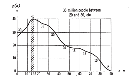
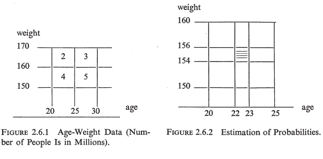
We are going to investigate situations in which we deal simultaneously with several random variables defined on the same sample space. As an introductory example, suppose that a person is selected at random from a certain population, and his age and weight recorded. We may take as the sample space the set of all pairs $(x, y)$ of real numbers, that is, the Euclidean plane $E^2$, where we interpret $x$ as the age and $y$ as the weight. Let $R_1$ be the age of the person selected, and $R_2$ the weight; that is, $R_1(x, y)=x, R_2(x, y)=y$. We wish to assign probabilities to events that involve $R_1$ and $R_2$ simultaneously. A cross-section of the available data might appear as shown in Figure 2.6.1. Thus there are 4 million people whose age is between 20 and 25 and (simultaneously) whose weight is between 150 and 160 pounds, and so on. Now suppose that we wish to estimate the number of people between 22 and 23 years, and 154 and 156 pounds. There are 4 million people spread over 5 years and 10 pounds, or 4/50 million per year-pound. We are interested in a range of 1 year and 2 pounds, and so our estimate is $4 / 50 \times 1 \times 2=8 / 50$ million (see Figure 2.6.2). If the total population is 200 million, then
$$
P\left{22 \leq R_1 \leq 23,154 \leq R_2 \leq 156\right}
$$
should be approximately
$$
\frac{8 / 50}{200}=.0008
$$
Notation. $\left{22 \leq R_1 \leq 23,154 \leq R_2 \leq 156\right}$ means $\left{22 \leq R_1 \leq 23\right.$ and $\left.154 \leq R_2 \leq 156\right}$.

数学代写|概率论代写Probability theory代考|Math561

概率论代考

数学代写|概率论代写Probability theory代考|PROPERTIES OF DISTRIBUTION FUNCTIONS

我们将建立任意随机变量的分布函数的一些一般性质。我们需要两个关于概率度量的事实。
定理1。设$(\Omega, \mathscr{F}, P)$为概率空间。
(a)如果$A_1, A_2, \ldots$是$\mathscr{F}$中集合的展开序列,即$A_n \subset A_{n+1}$适用于所有$n$,而$A=\bigcup_{n=1}^{\infty} A_n$则$P(A)=\lim _{n \rightarrow \infty} P\left(A_n\right)$。

(b)如果$A_1, A_2, \ldots$是$\mathscr{F}$中的集合的收缩序列,即$A_{n+1} \subset A_n$适用于所有$n$,而$A=\bigcap_{n=1}^{\infty} A_n$,则$P(A)=\lim {n \rightarrow \infty} P\left(A_n\right)$。证明。我们可以写$$ A=A_1 \cup\left(A_2-A_1\right) \cup\left(A_3-A_2\right) \cup \cdots \cup\left(A_n-A{n-1}\right) \cdots
$$
(见图2.5.1;注意,这是在展开序列的特殊情况下的展开(1.3.11)。由于这是一个分裂的联盟,
$$
\begin{aligned}
P(A) & =P\left(A_1\right)+P\left(A_2-A_1\right)+P\left(A_3-A_2\right)+\cdots \
& =P\left(A_1\right)+P\left(A_2\right)-P\left(A_1\right)+P\left(A_3\right)-P\left(A_2\right)+\cdots \quad \text { since } A_n \subset A_{n+1} \
& =\lim {n \rightarrow \infty} P\left(A_n\right) \end{aligned} $$ (b)如果$A=\bigcap{n=1}^{\infty} A_n$,则根据民主党法律,$A^c=\bigcup_{n=1}^{\infty} A_n{ }^c$。现在$A_{n+1} \subset A_n$;因此,$A_n{ }^c \subset A_{n+1}^c$。因此集合$A_n{ }^c$形成一个展开式序列,由(a), $P\left(A_n^c\right) \rightarrow P\left(A^c\right)$;那就是;$1-P\left(A_n\right) \rightarrow 1-P(A)$。结果如下。

数学代写|概率论代写Probability theory代考|JOINT DENSITY FUNCTIONS

我们将研究同时处理在同一样本空间上定义的几个随机变量的情况。作为一个介绍性的例子,假设从一定的人群中随机选择一个人,并记录他的年龄和体重。我们可以取实数对的集合$(x, y)$作为样本空间,即欧几里得平面$E^2$,其中$x$表示年龄,$y$表示权重。设$R_1$为入选人的年龄,$R_2$为权重;也就是$R_1(x, y)=x, R_2(x, y)=y$。我们希望为同时涉及$R_1$和$R_2$的事件分配概率。可用数据的横截面可能如图2.6.1所示。因此,有400万人的年龄在20到25岁之间,(同时)体重在150到160磅之间,以此类推。现在假设我们希望估计年龄在22到23岁之间,体重在154到156磅之间的人的数量。有400万人分布在5年和10英镑,或每年4/ 5000万英镑。我们对1年2磅的范围感兴趣,因此我们的估计是$4 / 50 \times 1 \times 2=8 / 50$百万(参见图2.6.2)。如果总人口是2亿,那么
$$
P\left{22 \leq R_1 \leq 23,154 \leq R_2 \leq 156\right}
$$
应该近似
$$
\frac{8 / 50}{200}=.0008
$$
符号。$\left{22 \leq R_1 \leq 23,154 \leq R_2 \leq 156\right}$分别代表$\left{22 \leq R_1 \leq 23\right.$和$\left.154 \leq R_2 \leq 156\right}$。

数学代写|概率论代写Probability theory代考 请认准statistics-lab™

统计代写请认准statistics-lab™. statistics-lab™为您的留学生涯保驾护航。

金融工程代写

金融工程是使用数学技术来解决金融问题。金融工程使用计算机科学、统计学、经济学和应用数学领域的工具和知识来解决当前的金融问题,以及设计新的和创新的金融产品。

非参数统计代写

非参数统计指的是一种统计方法,其中不假设数据来自于由少数参数决定的规定模型;这种模型的例子包括正态分布模型和线性回归模型。

广义线性模型代考

广义线性模型(GLM)归属统计学领域,是一种应用灵活的线性回归模型。该模型允许因变量的偏差分布有除了正态分布之外的其它分布。

术语 广义线性模型(GLM)通常是指给定连续和/或分类预测因素的连续响应变量的常规线性回归模型。它包括多元线性回归,以及方差分析和方差分析(仅含固定效应)。

有限元方法代写

有限元方法(FEM)是一种流行的方法,用于数值解决工程和数学建模中出现的微分方程。典型的问题领域包括结构分析、传热、流体流动、质量运输和电磁势等传统领域。

有限元是一种通用的数值方法,用于解决两个或三个空间变量的偏微分方程(即一些边界值问题)。为了解决一个问题,有限元将一个大系统细分为更小、更简单的部分,称为有限元。这是通过在空间维度上的特定空间离散化来实现的,它是通过构建对象的网格来实现的:用于求解的数值域,它有有限数量的点。边界值问题的有限元方法表述最终导致一个代数方程组。该方法在域上对未知函数进行逼近。[1] 然后将模拟这些有限元的简单方程组合成一个更大的方程系统,以模拟整个问题。然后,有限元通过变化微积分使相关的误差函数最小化来逼近一个解决方案。

tatistics-lab作为专业的留学生服务机构,多年来已为美国、英国、加拿大、澳洲等留学热门地的学生提供专业的学术服务,包括但不限于Essay代写,Assignment代写,Dissertation代写,Report代写,小组作业代写,Proposal代写,Paper代写,Presentation代写,计算机作业代写,论文修改和润色,网课代做,exam代考等等。写作范围涵盖高中,本科,研究生等海外留学全阶段,辐射金融,经济学,会计学,审计学,管理学等全球99%专业科目。写作团队既有专业英语母语作者,也有海外名校硕博留学生,每位写作老师都拥有过硬的语言能力,专业的学科背景和学术写作经验。我们承诺100%原创,100%专业,100%准时,100%满意。

随机分析代写


随机微积分是数学的一个分支,对随机过程进行操作。它允许为随机过程的积分定义一个关于随机过程的一致的积分理论。这个领域是由日本数学家伊藤清在第二次世界大战期间创建并开始的。

时间序列分析代写

随机过程,是依赖于参数的一组随机变量的全体,参数通常是时间。 随机变量是随机现象的数量表现,其时间序列是一组按照时间发生先后顺序进行排列的数据点序列。通常一组时间序列的时间间隔为一恒定值(如1秒,5分钟,12小时,7天,1年),因此时间序列可以作为离散时间数据进行分析处理。研究时间序列数据的意义在于现实中,往往需要研究某个事物其随时间发展变化的规律。这就需要通过研究该事物过去发展的历史记录,以得到其自身发展的规律。

回归分析代写

多元回归分析渐进(Multiple Regression Analysis Asymptotics)属于计量经济学领域,主要是一种数学上的统计分析方法,可以分析复杂情况下各影响因素的数学关系,在自然科学、社会和经济学等多个领域内应用广泛。

MATLAB代写

MATLAB 是一种用于技术计算的高性能语言。它将计算、可视化和编程集成在一个易于使用的环境中,其中问题和解决方案以熟悉的数学符号表示。典型用途包括:数学和计算算法开发建模、仿真和原型制作数据分析、探索和可视化科学和工程图形应用程序开发,包括图形用户界面构建MATLAB 是一个交互式系统,其基本数据元素是一个不需要维度的数组。这使您可以解决许多技术计算问题,尤其是那些具有矩阵和向量公式的问题,而只需用 C 或 Fortran 等标量非交互式语言编写程序所需的时间的一小部分。MATLAB 名称代表矩阵实验室。MATLAB 最初的编写目的是提供对由 LINPACK 和 EISPACK 项目开发的矩阵软件的轻松访问,这两个项目共同代表了矩阵计算软件的最新技术。MATLAB 经过多年的发展,得到了许多用户的投入。在大学环境中,它是数学、工程和科学入门和高级课程的标准教学工具。在工业领域,MATLAB 是高效研究、开发和分析的首选工具。MATLAB 具有一系列称为工具箱的特定于应用程序的解决方案。对于大多数 MATLAB 用户来说非常重要,工具箱允许您学习应用专业技术。工具箱是 MATLAB 函数(M 文件)的综合集合,可扩展 MATLAB 环境以解决特定类别的问题。可用工具箱的领域包括信号处理、控制系统、神经网络、模糊逻辑、小波、仿真等。

R语言代写问卷设计与分析代写
PYTHON代写回归分析与线性模型代写
MATLAB代写方差分析与试验设计代写
STATA代写机器学习/统计学习代写
SPSS代写计量经济学代写
EVIEWS代写时间序列分析代写
EXCEL代写深度学习代写
SQL代写各种数据建模与可视化代写

数学代写|概率论代写Probability theory代考|SF2940

如果你也在 怎样代写概率论Probability Theory 这个学科遇到相关的难题,请随时右上角联系我们的24/7代写客服。概率论Probability Theory是研究与随机现象有关的概率的数学分支。一个随机现象可能有几种结果。概率论用一定的形式概念描述某一特定结果发生的几率。

概率论Probability Theory某些随机变量在概率论中经常出现,因为它们很好地描述了许多自然或物理过程。因此,它们的分布在概率论中具有特殊的重要性。一些基本的离散分布有离散均匀分布、伯努利分布、二项式分布、负二项式分布、泊松分布和几何分布。重要的连续分布包括连续均匀分布、正态分布、指数分布、分布和分布。

statistics-lab™ 为您的留学生涯保驾护航 在代写概率论Probability theory方面已经树立了自己的口碑, 保证靠谱, 高质且原创的统计Statistics代写服务。我们的专家在代写概率论Probability theory代写方面经验极为丰富,各种代写概率论Probability theory相关的作业也就用不着说。

数学代写|概率论代写Probability theory代考|SF2940

数学代写|概率论代写Probability theory代考|APPENDIX: STIRLING’S FORMULA

An estimate of $n !$ that is of importance both in numerical calculations and theoretical analysis is Stirling’s formula
$$
n ! \sim n^n e^{-n} \sqrt{2 \pi n}
$$
in the sense that
$$
\lim {n \rightarrow \infty} \frac{n !}{\left(n^n e^{-n} \sqrt{2 \pi n}\right)}=1 $$ Proof. Define $(2 n) !$ ! (read $2 n$ semifactorial) as $2 n(2 n-2)(2 n-4) \cdots$ $6(4)(2)$, and $(2 n+1) ! !$ as $(2 n+1)(2 n-1) \cdots(5)(3)(1)$. We first show that (a) $$ \frac{(2 n) ! !}{(2 n+1) ! !}<\frac{\pi}{2} \frac{(2 n-1) ! !}{(2 n) ! !}<\frac{(2 n-2) ! !}{(2 n-1) ! !} $$ Let $I_k=\int_0^{\pi / 2}(\cos x)^k d x, k=0,1,2, \ldots$ Then $I_0=\pi / 2, I_1=1$. Integrating by parts, we obtain $I_k=\int_0^{\pi / 2}(\cos x)^{k-1} d(\sin x)=\int_0^{\pi / 2}(k-1)(\cos x)^{k-2}$ $\sin ^2 x d x$. Since $\sin ^2 x=1-\cos ^2 x$, we have $I_k=(k-1) I{k-2}-(k-1) I_k$ or $I_k=[(k-1) / k] I_{k-2}$. By iteration, we obtain $I_{2 n}=(\pi / 2)[(2 n-1) ! ! /$ $(2 n) ! !]$ and $I_{2 n+1}=[(2 n) ! ! /(2 n+1) ! !]$. Since $(\cos x)^k$ decreases with $k$, so does $I_k$, and hence $I_{2 n+1}<I_{2 n}<I_{2 n-1}$, and (a) is proved.
(b) Let $Q_n=\left(\begin{array}{c}2^n \ n\end{array}\right) / 2^{2 n}$. Then
$$
\lim _{n \rightarrow \infty} Q_n \sqrt{n \pi}=1
$$
To prove this, write
$$
\begin{aligned}
Q_n & =\frac{(2 n) !}{n ! n ! 2^{2 n}}=\frac{(2 n) !}{\left(2^n n !\right)^2} \
& =\frac{(2 n) !}{((2 n)(2 n-2) \cdots(4)(2))^2}=\frac{(2 n-1) ! !}{(2 n) ! !}
\end{aligned}
$$

Thus, by (a),
$$
\frac{(2 n) ! !}{(2 n+1) ! !}<\frac{\pi}{2} Q_n<\frac{(2 n-2) ! !}{(2 n-1) ! !}
$$
Multiply this inequality by
$$
\frac{(2 n-1) ! !}{(2 n-2) ! !}=\frac{(2 n-1) ! !}{(2 n) ! !} \frac{(2 n) ! !}{(2 n-2) ! !}=Q_n(2 n)
$$
to obtain
$$
\frac{2 n}{2 n+1}<n \pi Q_n{ }^2<1
$$
If we let $n \rightarrow \infty$, we obtain $n \pi Q_n{ }^2 \rightarrow 1$, proving (b).
(c) Proof of Stirling’s formula. Let $c_n=n ! / n^n e^{-n} \sqrt{2 \pi n}$. We must show that $c_n \rightarrow 1$ as $n \rightarrow \infty$. Consider $(n+1) ! / n !=n+1$. We have
$$
\begin{aligned}
\frac{(n+1) !}{n !} & =\frac{c_{n+1}(n+1)^{n+1} e^{-(n+1)} \sqrt{2 \pi(n+1)}}{c_n n^n e^{-n} \sqrt{2 \pi n}} \
& =\left(\frac{c_{n+1}}{c_n}\right) e^{-1}\left(\frac{n+1}{n}\right)^n \frac{(n+1)^{3 / 2}}{\sqrt{n}}
\end{aligned}
$$

数学代写|概率论代写Probability theory代考|DEFINITION OF A RANDOM VARIABLE

Intuitively, a random variable is a quantity that is measured in connection with a random experiment. If $\Omega$ is a sample space, and the outcome of the experiment is $\omega$, a measuring process is carried out to obtain a number $R(\omega)$. Thus a random variable is a real-valued function on a sample space. (The formal definition, which is postponed until later in the section, is somewhat more restrictive.)

Example 1. Throw a coin 10 times, and let $R$ be the number of heads. We take $\Omega=$ all sequences of length 10 with components $H$ and $T ; 2^{10}$ points altogether. A typical sample point is $\omega=H H T H T T H H T H$. For this point $R(\omega)=6$. Another random variable, $R_1$, is the number of times a head is followed immediately by a tail. For the point $\omega$ above, $R_1(\omega)=3$.
Example 2. Pick a person at random from a certain population and measure his height and weight. We may take the sample space to be the plane $E^2$, that is, the set of all pairs $(x, y)$ of real numbers, with the first coordinate $x$ representing the height and the second coordinate $y$ the weight (we can take care of the requirement that height and weight be nonnegative by assigning probability 0 to the complement of the first quadrant). Let $R_1$ be the height of the person selected, and let $R_2$ be the weight. Then $R_1(x, y)=x, R_2(x, y)=y$. As another example, let $R_3$ be twice the height plus the cube root of the weight; that is, $R_3=2 R_1+\sqrt[3]{R_2}$. Then $R_3(x, y)=$ $2 R_1(x, y)+\sqrt[3]{R_2(x, y)}=2 x+\sqrt[3]{y}$.

Example 3. Throw two dice. We may take the sample space to be the set of all pairs of integers $(x, y), x, y=1,2, \ldots, 6$ (36 points in all).
Let $R_1=$ the result of the first toss. Then $R_1(x, y)=x$.
Let $R_2=$ the sum of the two faces. Then $R_2(x, y)=x+y$.
Let $R_3=1$ if at least one face is an even number; $R_3=0$ otherwise.
Then $R_3(6,5)=1 ; R_3(3,6)=1 ; R_3(1,3)=0$, and so on.

数学代写|概率论代写Probability theory代考|SF2940

概率论代考

数学代写|概率论代写Probability theory代考|APPENDIX: STIRLING’S FORMULA

在数值计算和理论分析中都很重要的对$n !$的估计是斯特林公式
$$
n ! \sim n^n e^{-n} \sqrt{2 \pi n}
$$
从某种意义上说
$$
\lim {n \rightarrow \infty} \frac{n !}{\left(n^n e^{-n} \sqrt{2 \pi n}\right)}=1 $$证明。定义$(2 n) !$ !(读取$2 n$半阶乘)为$2 n(2 n-2)(2 n-4) \cdots$$6(4)(2)$, $(2 n+1) ! !$为$(2 n+1)(2 n-1) \cdots(5)(3)(1)$。我们首先表明(a) $$ \frac{(2 n) ! !}{(2 n+1) ! !}<\frac{\pi}{2} \frac{(2 n-1) ! !}{(2 n) ! !}<\frac{(2 n-2) ! !}{(2 n-1) ! !} $$让$I_k=\int_0^{\pi / 2}(\cos x)^k d x, k=0,1,2, \ldots$然后$I_0=\pi / 2, I_1=1$。分部积分,得到$I_k=\int_0^{\pi / 2}(\cos x)^{k-1} d(\sin x)=\int_0^{\pi / 2}(k-1)(\cos x)^{k-2}$$\sin ^2 x d x$。因为$\sin ^2 x=1-\cos ^2 x$,我们有$I_k=(k-1) I{k-2}-(k-1) I_k$或$I_k=[(k-1) / k] I_{k-2}$。通过迭代得到$I_{2 n}=(\pi / 2)[(2 n-1) ! ! /$$(2 n) ! !]$和$I_{2 n+1}=[(2 n) ! ! /(2 n+1) ! !]$。由于$(\cos x)^k$随$k$减小,$I_k$也减小,因此$I_{2 n+1}<I_{2 n}<I_{2 n-1}$得到证明。
(b)让$Q_n=\left(\begin{array}{c}2^n \ n\end{array}\right) / 2^{2 n}$。然后
$$
\lim _{n \rightarrow \infty} Q_n \sqrt{n \pi}=1
$$
为了证明这一点,写下来
$$
\begin{aligned}
Q_n & =\frac{(2 n) !}{n ! n ! 2^{2 n}}=\frac{(2 n) !}{\left(2^n n !\right)^2} \
& =\frac{(2 n) !}{((2 n)(2 n-2) \cdots(4)(2))^2}=\frac{(2 n-1) ! !}{(2 n) ! !}
\end{aligned}
$$

因此,通过(a),
$$
\frac{(2 n) ! !}{(2 n+1) ! !}<\frac{\pi}{2} Q_n<\frac{(2 n-2) ! !}{(2 n-1) ! !}
$$
将这个不等式乘以
$$
\frac{(2 n-1) ! !}{(2 n-2) ! !}=\frac{(2 n-1) ! !}{(2 n) ! !} \frac{(2 n) ! !}{(2 n-2) ! !}=Q_n(2 n)
$$
获取
$$
\frac{2 n}{2 n+1}<n \pi Q_n{ }^2<1
$$
令$n \rightarrow \infty$,得到$n \pi Q_n{ }^2 \rightarrow 1$,证明(b)。
(c)斯特林公式的证明。让$c_n=n ! / n^n e^{-n} \sqrt{2 \pi n}$。我们必须将$c_n \rightarrow 1$表示为$n \rightarrow \infty$。考虑$(n+1) ! / n !=n+1$。我们有
$$
\begin{aligned}
\frac{(n+1) !}{n !} & =\frac{c_{n+1}(n+1)^{n+1} e^{-(n+1)} \sqrt{2 \pi(n+1)}}{c_n n^n e^{-n} \sqrt{2 \pi n}} \
& =\left(\frac{c_{n+1}}{c_n}\right) e^{-1}\left(\frac{n+1}{n}\right)^n \frac{(n+1)^{3 / 2}}{\sqrt{n}}
\end{aligned}
$$

数学代写|概率论代写Probability theory代考|DEFINITION OF A RANDOM VARIABLE

直观地说,随机变量是在随机实验中测量的量。如果$\Omega$是一个样本空间,实验结果为$\omega$,则进行测量过程,得到一个数字$R(\omega)$。因此,随机变量是样本空间上的实值函数。(正式的定义将推迟到本节后面的部分,它在某种程度上更具限制性。)

例1。投掷硬币10次,设$R$为正面的次数。我们取$\Omega=$所有长度为10的序列,其组成部分为$H$和$T ; 2^{10}$。一个典型的样本点是$\omega=H H T H T T H H T H$。对于这一点$R(\omega)=6$。另一个随机变量$R_1$是正面紧接着反面的次数。对于上面的$\omega$点,$R_1(\omega)=3$。
例2。从一定的人群中随机挑选一个人,测量他的身高和体重。我们可以将样本空间作为平面$E^2$,即所有实数对$(x, y)$的集合,第一个坐标$x$表示高度,第二个坐标$y$表示权重(我们可以通过为第一象限的补赋概率0来满足高度和权重非负的要求)。设$R_1$为被选者的身高,$R_2$为体重。然后$R_1(x, y)=x, R_2(x, y)=y$。另一个例子,设$R_3$等于两倍的高度加上重量的立方根;也就是$R_3=2 R_1+\sqrt[3]{R_2}$。然后是$R_3(x, y)=$$2 R_1(x, y)+\sqrt[3]{R_2(x, y)}=2 x+\sqrt[3]{y}$。

例3。掷两个骰子。我们可以取样本空间为所有整数对的集合$(x, y), x, y=1,2, \ldots, 6$(总共36个点)。
让$R_1=$公布第一次掷硬币的结果。然后$R_1(x, y)=x$。
设$R_2=$为两个面之和。然后$R_2(x, y)=x+y$。
设$R_3=1$,如果至少有一个面是偶数;$R_3=0$否则。
然后是$R_3(6,5)=1 ; R_3(3,6)=1 ; R_3(1,3)=0$,等等。

数学代写|概率论代写Probability theory代考 请认准statistics-lab™

统计代写请认准statistics-lab™. statistics-lab™为您的留学生涯保驾护航。

金融工程代写

金融工程是使用数学技术来解决金融问题。金融工程使用计算机科学、统计学、经济学和应用数学领域的工具和知识来解决当前的金融问题,以及设计新的和创新的金融产品。

非参数统计代写

非参数统计指的是一种统计方法,其中不假设数据来自于由少数参数决定的规定模型;这种模型的例子包括正态分布模型和线性回归模型。

广义线性模型代考

广义线性模型(GLM)归属统计学领域,是一种应用灵活的线性回归模型。该模型允许因变量的偏差分布有除了正态分布之外的其它分布。

术语 广义线性模型(GLM)通常是指给定连续和/或分类预测因素的连续响应变量的常规线性回归模型。它包括多元线性回归,以及方差分析和方差分析(仅含固定效应)。

有限元方法代写

有限元方法(FEM)是一种流行的方法,用于数值解决工程和数学建模中出现的微分方程。典型的问题领域包括结构分析、传热、流体流动、质量运输和电磁势等传统领域。

有限元是一种通用的数值方法,用于解决两个或三个空间变量的偏微分方程(即一些边界值问题)。为了解决一个问题,有限元将一个大系统细分为更小、更简单的部分,称为有限元。这是通过在空间维度上的特定空间离散化来实现的,它是通过构建对象的网格来实现的:用于求解的数值域,它有有限数量的点。边界值问题的有限元方法表述最终导致一个代数方程组。该方法在域上对未知函数进行逼近。[1] 然后将模拟这些有限元的简单方程组合成一个更大的方程系统,以模拟整个问题。然后,有限元通过变化微积分使相关的误差函数最小化来逼近一个解决方案。

tatistics-lab作为专业的留学生服务机构,多年来已为美国、英国、加拿大、澳洲等留学热门地的学生提供专业的学术服务,包括但不限于Essay代写,Assignment代写,Dissertation代写,Report代写,小组作业代写,Proposal代写,Paper代写,Presentation代写,计算机作业代写,论文修改和润色,网课代做,exam代考等等。写作范围涵盖高中,本科,研究生等海外留学全阶段,辐射金融,经济学,会计学,审计学,管理学等全球99%专业科目。写作团队既有专业英语母语作者,也有海外名校硕博留学生,每位写作老师都拥有过硬的语言能力,专业的学科背景和学术写作经验。我们承诺100%原创,100%专业,100%准时,100%满意。

随机分析代写


随机微积分是数学的一个分支,对随机过程进行操作。它允许为随机过程的积分定义一个关于随机过程的一致的积分理论。这个领域是由日本数学家伊藤清在第二次世界大战期间创建并开始的。

时间序列分析代写

随机过程,是依赖于参数的一组随机变量的全体,参数通常是时间。 随机变量是随机现象的数量表现,其时间序列是一组按照时间发生先后顺序进行排列的数据点序列。通常一组时间序列的时间间隔为一恒定值(如1秒,5分钟,12小时,7天,1年),因此时间序列可以作为离散时间数据进行分析处理。研究时间序列数据的意义在于现实中,往往需要研究某个事物其随时间发展变化的规律。这就需要通过研究该事物过去发展的历史记录,以得到其自身发展的规律。

回归分析代写

多元回归分析渐进(Multiple Regression Analysis Asymptotics)属于计量经济学领域,主要是一种数学上的统计分析方法,可以分析复杂情况下各影响因素的数学关系,在自然科学、社会和经济学等多个领域内应用广泛。

MATLAB代写

MATLAB 是一种用于技术计算的高性能语言。它将计算、可视化和编程集成在一个易于使用的环境中,其中问题和解决方案以熟悉的数学符号表示。典型用途包括:数学和计算算法开发建模、仿真和原型制作数据分析、探索和可视化科学和工程图形应用程序开发,包括图形用户界面构建MATLAB 是一个交互式系统,其基本数据元素是一个不需要维度的数组。这使您可以解决许多技术计算问题,尤其是那些具有矩阵和向量公式的问题,而只需用 C 或 Fortran 等标量非交互式语言编写程序所需的时间的一小部分。MATLAB 名称代表矩阵实验室。MATLAB 最初的编写目的是提供对由 LINPACK 和 EISPACK 项目开发的矩阵软件的轻松访问,这两个项目共同代表了矩阵计算软件的最新技术。MATLAB 经过多年的发展,得到了许多用户的投入。在大学环境中,它是数学、工程和科学入门和高级课程的标准教学工具。在工业领域,MATLAB 是高效研究、开发和分析的首选工具。MATLAB 具有一系列称为工具箱的特定于应用程序的解决方案。对于大多数 MATLAB 用户来说非常重要,工具箱允许您学习应用专业技术。工具箱是 MATLAB 函数(M 文件)的综合集合,可扩展 MATLAB 环境以解决特定类别的问题。可用工具箱的领域包括信号处理、控制系统、神经网络、模糊逻辑、小波、仿真等。

R语言代写问卷设计与分析代写
PYTHON代写回归分析与线性模型代写
MATLAB代写方差分析与试验设计代写
STATA代写机器学习/统计学习代写
SPSS代写计量经济学代写
EVIEWS代写时间序列分析代写
EXCEL代写深度学习代写
SQL代写各种数据建模与可视化代写

数学代写|概率论代写Probability theory代考|MAP4102

如果你也在 怎样代写概率论Probability Theory 这个学科遇到相关的难题,请随时右上角联系我们的24/7代写客服。概率论Probability Theory是研究与随机现象有关的概率的数学分支。一个随机现象可能有几种结果。概率论用一定的形式概念描述某一特定结果发生的几率。

概率论Probability Theory某些随机变量在概率论中经常出现,因为它们很好地描述了许多自然或物理过程。因此,它们的分布在概率论中具有特殊的重要性。一些基本的离散分布有离散均匀分布、伯努利分布、二项式分布、负二项式分布、泊松分布和几何分布。重要的连续分布包括连续均匀分布、正态分布、指数分布、分布和分布。

statistics-lab™ 为您的留学生涯保驾护航 在代写概率论Probability theory方面已经树立了自己的口碑, 保证靠谱, 高质且原创的统计Statistics代写服务。我们的专家在代写概率论Probability theory代写方面经验极为丰富,各种代写概率论Probability theory相关的作业也就用不着说。

数学代写|概率论代写Probability theory代考|MAP4102

数学代写|概率论代写Probability theory代考|COMBINATORIAL PROBLEMS

We consider a class of problems in which the assignment of probabilities can be made in a natural way.

Let $\Omega$ be a finite or countably infinite set, and let $\mathscr{F}$ consist of all subsets of $\Omega$.

For each point $\omega_i \in \Omega, i=1,2, \ldots$, assign a nonnegative number $p_i$, with $\sum_i p_i=1$. If $A$ is any subset of $\Omega$, let $P(A)=\sum_{\omega_i \in A} p_i$. Then it may be verified that $P$ is a probability measure; $P\left{\omega_i\right}=p_i$, and the probability of any event $A$ is found by adding the probabilities of the points of $A$. An $(\Omega, \mathscr{F}, P)$ of this type is called a discrete probability space.
Example 1. Throw a (biased) coin twice (see Figure 1.4.1).
Let $E_1=$ {at least one head $}$. Then
$$
E_1=A_1 \cup A_2 \cup A_3
$$
Hence
$$
\begin{aligned}
P\left(E_1\right) & =P\left(A_1\right)+P\left(A_2\right)+P\left(A_3\right) \
& =.36+.24+.24=.84
\end{aligned}
$$
Let $E_2=$ {tail on first toss $}$; then
$$
E_2=A_3 \cup A_4
$$

and
$$
P\left(E_2\right)=P\left(A_3\right)+P\left(A_4\right)=.4
$$
In the special case when $\Omega=\left{\omega_1, \ldots, \omega_n\right}$ and $p_i=1 / n, i=1,2, \ldots, n$, we have
$$
P(A)=\frac{\text { number of points of } A}{\text { total number of points in } \Omega}=\frac{\text { favorable outcomes }}{\text { total outcomes }}
$$
corresponding to the classical definition of probability.

数学代写|概率论代写Probability theory代考|Ordered samples of size $r$, with replacement

The number of ordered sequences $\left(a_{i_1}, \ldots, a_{i_r}\right)$, where the $a_{i_k}$ belong to $\left{a_1, \ldots, a_n\right}$, is $n \times n \times \cdots \times n$ ( $r$ times), or
$$
n^r
$$
(The term “with replacement” refers to the fact that if the symbol $a_{i_k}$ is selected at step $k$ it may be selected again at any future time.)

For example, the number of possible outcomes if three dice are thrown is $6 \times 6 \times 6=216$.
Ordered Samples of Size $r$, without Replacement
The number of ordered sequences $\left(a_{i_1}, \ldots, a_{i_r}\right)$, where the $a_{i_k}$ belong to $\left{a_1, \ldots, a_n\right}$, but repetition is not allowed (i.e., no $a_i$ can appear more than once in the sequence), is
$$
n(n-1) \cdots(n-r+1)=\frac{n !}{(n-r) !}, \quad r=1,2, \ldots, n
$$
(The first symbol may be chosen in $n$ ways, and the second in $n-1$ ways, since the first symbol may not be used again, and so on.) The above number is sometimes called the number of permutations of $r$ objects out of $n$, written $(n)_r$.

For example, the number of 3-digit numbers that can be formed from $1,2, \ldots, 9$, if no digit can be repeated, is $9(8)(7)=504$.

Unordered Samples of Size $r$, without Replacement
The number of unordered sets $\left{a_{i_1}, \ldots, a_{i_r}\right}$, where the $a_{i_k}, k=1, \ldots, r$, are distinct elements of $\left{a_1, \ldots, a_n\right}$ (i.e., the number of ways of selecting $r$ distinct objects out of $n$ ), if order does not count, is
$$
\left(\begin{array}{l}
n \
r
\end{array}\right)=\frac{n !}{r !(n-r) !}
$$
To see this, consider the following process.
(a) Select $r$ distinct objects out of $n$ without regard to order; this can be done in $\left(\begin{array}{l}n \ r\end{array}\right)$ ways, where $\left(\begin{array}{l}n \ r\end{array}\right)$ is to be determined.
(b) For each set selected in (a), say $\left{a_{i_1}, \ldots, a_{i_r}\right}$, select an ordering of $a_{i_1}, \ldots, a_{i_r}$. This can be done in $(r)_r=r$ ! ways (see Figure 1.4.2 for $n=3$, $r=2)$.

The result of performing (a) and (b) is a permutation of $r$ objects out of $n$; hence
$$
\left(\begin{array}{l}
n \
r
\end{array}\right) r !=(n)_r=\frac{n !}{(n-r) !}
$$
or
$$
\left(\begin{array}{l}
n \
r
\end{array}\right)=\frac{n !}{r !(n-r) !}, \quad r=1,2, \ldots, n
$$
We define $\left(\begin{array}{l}n \ 0\end{array}\right)$ to be $n ! / 0 ! n !=1$, to make the formula for $\left(\begin{array}{l}n \ r\end{array}\right)$ valid for $r=0,1, \ldots, n$. Notice that $\left(\begin{array}{c}n \ k\end{array}\right)=\left(\begin{array}{c}n \ n-k\end{array}\right)$.

数学代写|概率论代写Probability theory代考|MAP4102

概率论代考

数学代写|概率论代写Probability theory代考|COMBINATORIAL PROBLEMS

我们考虑一类问题,其中概率的分配可以用一种自然的方式进行。

设$\ ω $是一个有限或可数无限集,且设$\mathscr{F}$由$\ ω $的所有子集组成。

对于每个点$\omega_i \in \omega_i, i=1,2, \ldots$,赋一个非负数$p_i$,其中$\sum_i p_i=1$。如果$A$是$\Omega$的任意子集,令$P(A)=\sum_{\omega_i \in A} p_i$。然后可以验证$P$是一个概率测度;$P\left{\omega_i\right}=p_i$,任意事件$A$的概率通过将$A$各点的概率相加得到。这种类型的$(\Omega, \mathscr{F}, P)$称为离散概率空间。
例1。投掷一枚(有偏的)硬币两次(见图1.4.1)。
设$E_1=${至少一个头部$}$。然后


$$
P\left(E_2\right)=P\left(A_3\right)+P\left(A_4\right)=.4
$$
在$\Omega=\left{\omega_1, \ldots, \omega_n\right}$和$p_i=1 / n, i=1,2, \ldots, n$的特殊情况下,我们有
$$
P(A)=\frac{\text { number of points of } A}{\text { total number of points in } \Omega}=\frac{\text { favorable outcomes }}{\text { total outcomes }}
$$
对应于概率的经典定义。

数学代写|概率论代写Probability theory代考|Ordered samples of size $r$, with replacement

有序序列的数目 $\left(a_{i_1}, \ldots, a_{i_r}\right)$,其中 $a_{i_k}$ 属于 $\left{a_1, \ldots, a_n\right}$是吗? $n \times n \times \cdots \times n$ ( $r$ 次数),或
$$
n^r
$$
(术语“与替换”是指如果符号 $a_{i_k}$ 在第一步被选中 $k$ 可在将来任何时候再次选择。)

例如,如果投掷三个骰子,可能的结果数是$6 \times 6 \times 6=216$。
订购样品尺寸$r$,不得更换
有序序列$\left(a_{i_1}, \ldots, a_{i_r}\right)$的个数为,其中$a_{i_k}$属于$\left{a_1, \ldots, a_n\right}$,但不允许重复(即$a_i$不能在序列中出现多次)
$$
n(n-1) \cdots(n-r+1)=\frac{n !}{(n-r) !}, \quad r=1,2, \ldots, n
$$
(第一个符号可以以$n$的方式选择,第二个符号可以以$n-1$的方式选择,因为第一个符号可能不会再次使用,以此类推。)上述数字有时称为$r$对象对$n$的排列次数,写为$(n)_r$。

例如,$1,2, \ldots, 9$可以组成的3位数个数,如果不能重复,则为$9(8)(7)=504$。

未订购的样品尺寸$r$,无更换
无序集合$\left{a_{i_1}, \ldots, a_{i_r}\right}$的数量,其中$a_{i_k}, k=1, \ldots, r$是$\left{a_1, \ldots, a_n\right}$的不同元素(即,从$n$中选择$r$不同对象的方法的数量),如果不考虑顺序,则为
$$
\left(\begin{array}{l}
n \
r
\end{array}\right)=\frac{n !}{r !(n-r) !}
$$
要了解这一点,请考虑以下过程。
(a)从$n$中不顾顺序选择$r$不同的对象;这可以通过$\left(\begin{array}{l}n \ r\end{array}\right)$方式完成,其中$\left(\begin{array}{l}n \ r\end{array}\right)$是要确定的。
(b)对于(a)中选择的每个集合,例如$\left{a_{i_1}, \ldots, a_{i_r}\right}$,选择一个$a_{i_1}, \ldots, a_{i_r}$的排序。这可以在$(r)_r=r$完成!方式($n=3$, $r=2)$见图1.4.2)。

执行(a)和(b)的结果是$n$中$r$对象的排列;因此
$$
\left(\begin{array}{l}
n \
r
\end{array}\right) r !=(n)_r=\frac{n !}{(n-r) !}
$$

$$
\left(\begin{array}{l}
n \
r
\end{array}\right)=\frac{n !}{r !(n-r) !}, \quad r=1,2, \ldots, n
$$
我们将$\left(\begin{array}{l}n \ 0\end{array}\right)$定义为$n ! / 0 ! n !=1$,以使$\left(\begin{array}{l}n \ r\end{array}\right)$的公式对$r=0,1, \ldots, n$有效。注意$\left(\begin{array}{c}n \ k\end{array}\right)=\left(\begin{array}{c}n \ n-k\end{array}\right)$。

数学代写|概率论代写Probability theory代考 请认准statistics-lab™

统计代写请认准statistics-lab™. statistics-lab™为您的留学生涯保驾护航。

金融工程代写

金融工程是使用数学技术来解决金融问题。金融工程使用计算机科学、统计学、经济学和应用数学领域的工具和知识来解决当前的金融问题,以及设计新的和创新的金融产品。

非参数统计代写

非参数统计指的是一种统计方法,其中不假设数据来自于由少数参数决定的规定模型;这种模型的例子包括正态分布模型和线性回归模型。

广义线性模型代考

广义线性模型(GLM)归属统计学领域,是一种应用灵活的线性回归模型。该模型允许因变量的偏差分布有除了正态分布之外的其它分布。

术语 广义线性模型(GLM)通常是指给定连续和/或分类预测因素的连续响应变量的常规线性回归模型。它包括多元线性回归,以及方差分析和方差分析(仅含固定效应)。

有限元方法代写

有限元方法(FEM)是一种流行的方法,用于数值解决工程和数学建模中出现的微分方程。典型的问题领域包括结构分析、传热、流体流动、质量运输和电磁势等传统领域。

有限元是一种通用的数值方法,用于解决两个或三个空间变量的偏微分方程(即一些边界值问题)。为了解决一个问题,有限元将一个大系统细分为更小、更简单的部分,称为有限元。这是通过在空间维度上的特定空间离散化来实现的,它是通过构建对象的网格来实现的:用于求解的数值域,它有有限数量的点。边界值问题的有限元方法表述最终导致一个代数方程组。该方法在域上对未知函数进行逼近。[1] 然后将模拟这些有限元的简单方程组合成一个更大的方程系统,以模拟整个问题。然后,有限元通过变化微积分使相关的误差函数最小化来逼近一个解决方案。

tatistics-lab作为专业的留学生服务机构,多年来已为美国、英国、加拿大、澳洲等留学热门地的学生提供专业的学术服务,包括但不限于Essay代写,Assignment代写,Dissertation代写,Report代写,小组作业代写,Proposal代写,Paper代写,Presentation代写,计算机作业代写,论文修改和润色,网课代做,exam代考等等。写作范围涵盖高中,本科,研究生等海外留学全阶段,辐射金融,经济学,会计学,审计学,管理学等全球99%专业科目。写作团队既有专业英语母语作者,也有海外名校硕博留学生,每位写作老师都拥有过硬的语言能力,专业的学科背景和学术写作经验。我们承诺100%原创,100%专业,100%准时,100%满意。

随机分析代写


随机微积分是数学的一个分支,对随机过程进行操作。它允许为随机过程的积分定义一个关于随机过程的一致的积分理论。这个领域是由日本数学家伊藤清在第二次世界大战期间创建并开始的。

时间序列分析代写

随机过程,是依赖于参数的一组随机变量的全体,参数通常是时间。 随机变量是随机现象的数量表现,其时间序列是一组按照时间发生先后顺序进行排列的数据点序列。通常一组时间序列的时间间隔为一恒定值(如1秒,5分钟,12小时,7天,1年),因此时间序列可以作为离散时间数据进行分析处理。研究时间序列数据的意义在于现实中,往往需要研究某个事物其随时间发展变化的规律。这就需要通过研究该事物过去发展的历史记录,以得到其自身发展的规律。

回归分析代写

多元回归分析渐进(Multiple Regression Analysis Asymptotics)属于计量经济学领域,主要是一种数学上的统计分析方法,可以分析复杂情况下各影响因素的数学关系,在自然科学、社会和经济学等多个领域内应用广泛。

MATLAB代写

MATLAB 是一种用于技术计算的高性能语言。它将计算、可视化和编程集成在一个易于使用的环境中,其中问题和解决方案以熟悉的数学符号表示。典型用途包括:数学和计算算法开发建模、仿真和原型制作数据分析、探索和可视化科学和工程图形应用程序开发,包括图形用户界面构建MATLAB 是一个交互式系统,其基本数据元素是一个不需要维度的数组。这使您可以解决许多技术计算问题,尤其是那些具有矩阵和向量公式的问题,而只需用 C 或 Fortran 等标量非交互式语言编写程序所需的时间的一小部分。MATLAB 名称代表矩阵实验室。MATLAB 最初的编写目的是提供对由 LINPACK 和 EISPACK 项目开发的矩阵软件的轻松访问,这两个项目共同代表了矩阵计算软件的最新技术。MATLAB 经过多年的发展,得到了许多用户的投入。在大学环境中,它是数学、工程和科学入门和高级课程的标准教学工具。在工业领域,MATLAB 是高效研究、开发和分析的首选工具。MATLAB 具有一系列称为工具箱的特定于应用程序的解决方案。对于大多数 MATLAB 用户来说非常重要,工具箱允许您学习应用专业技术。工具箱是 MATLAB 函数(M 文件)的综合集合,可扩展 MATLAB 环境以解决特定类别的问题。可用工具箱的领域包括信号处理、控制系统、神经网络、模糊逻辑、小波、仿真等。

R语言代写问卷设计与分析代写
PYTHON代写回归分析与线性模型代写
MATLAB代写方差分析与试验设计代写
STATA代写机器学习/统计学习代写
SPSS代写计量经济学代写
EVIEWS代写时间序列分析代写
EXCEL代写深度学习代写
SQL代写各种数据建模与可视化代写

数学代写|概率论代写Probability theory代考|DTSA5001

如果你也在 怎样代写概率论Probability Theory 这个学科遇到相关的难题,请随时右上角联系我们的24/7代写客服。概率论Probability Theory是研究与随机现象有关的概率的数学分支。一个随机现象可能有几种结果。概率论用一定的形式概念描述某一特定结果发生的几率。

概率论Probability Theory某些随机变量在概率论中经常出现,因为它们很好地描述了许多自然或物理过程。因此,它们的分布在概率论中具有特殊的重要性。一些基本的离散分布有离散均匀分布、伯努利分布、二项式分布、负二项式分布、泊松分布和几何分布。重要的连续分布包括连续均匀分布、正态分布、指数分布、分布和分布。

statistics-lab™ 为您的留学生涯保驾护航 在代写概率论Probability theory方面已经树立了自己的口碑, 保证靠谱, 高质且原创的统计Statistics代写服务。我们的专家在代写概率论Probability theory代写方面经验极为丰富,各种代写概率论Probability theory相关的作业也就用不着说。

数学代写|概率论代写Probability theory代考|DTSA5001

数学代写|概率论代写Probability theory代考|VARIABLE DISTRIBUTIONS

$\mathrm{Up}$ to now we have considered only variables $\mathbf{X}_k$ having the same distribution. This situation corresponds to a repetition of the same game of chance, but it is more interesting to see what happens if the type of game changes at each step. It is not necessary to think of gambling places; the statistician who applies statistical tests is engaged in a dignified sort of gambling, and in his case the distribution of the random variables changes from occasion to occasion.

To fix ideas we shall imagine that an infinite sequence of probability distributions is given so that for each $n$ we have $n$ mutually independent variables $\mathbf{X}_1, \ldots, \mathbf{X}_n$ with the prescribed distributions. We assume that the means and variances exist and put
$$
\mu_k=\mathbf{E}\left(\mathbf{X}_k\right), \quad \sigma_k^2=\operatorname{Var}\left(\mathbf{X}_k\right)
$$
The sum $\mathbf{S}_n=\mathbf{X}_1+\cdots+\mathbf{X}_n$ has mean $m_n$ and variance $s_n^2$ given by
$$
m_n=\mu_1+\cdots+\mu_n, \quad s_n^2=\sigma_1^2+\cdots+\sigma_n^2
$$

[cf. IX, (2.4) and IX,(5.6)]. In the special case of identical distributions we had $m_n=n \mu, s_n^2=n \sigma^2$.

The (weak) law of large numbers is said to hold for the sequence $\left{\mathbf{X}_k\right}$ if for every $\epsilon>0$
$$
\mathbf{P}\left{\frac{\left|\mathbf{S}_n-m_n\right|}{n}>\epsilon\right} \rightarrow 0 .
$$
The sequence $\left{\mathbf{X}_k\right}$ is said to obey the central limit theorem if for every fixed $\alpha<\beta$
$$
\mathbf{P}\left{\alpha<\frac{\mathbf{S}_n-m_n}{s_n}<\beta\right} \rightarrow \mathfrak{N}(\beta)-\mathfrak{N}(\alpha) .
$$
It is one of the salient features of probability theory that both the law of large numbers and the central limit theorem hold for a surprisingly large class of sequences $\left{\mathbf{X}_k\right}$. In particular, the law of large numbers halds. whenever the $\mathbf{X}_k$ are uniformly bounded, that is, whenever there cxists a constant $A$ such that $\left.\rfloor \mathbf{X}_k\right\rfloor<A$ for all $k$. More generally, a sufficient condition for the law of large numbers to hold is that
$$
\frac{s_n}{n} \rightarrow 0 .
$$

数学代写|概率论代写Probability theory代考|APPLICATIONS TO COMBINATORIAL ANALYSIS

We shall give two examples of applications of the central limit theorem to problems not directly connected with probability theory. Both relate to the $n$ ! permutations of the $n$ elements $a_1, a_2, \ldots, a_n$, to each of which we attribute probability $1 / n$ !.
(a) Inversions. In a given permutation the element $a_k$ is said to induce $r$ inversions if it precedes exactly $r$ elements with smaller index (i.e., elements which precede $a_k$ in the natural order). For example, in $\left(a_3 a_6 a_1 a_5 a_2 a_4\right)$ the elements $a_1$ and $a_2$ induce no inversion, $a_3$ induces two, $a_4$ none, $a_5$ two, and $a_6$ four. In $\left(a_6 a_5 a_4 a_3 a_2 a_1\right)$ the element $a_k$ induces $k-1$ inversions and there are fifteen inversions in all. The number $\mathbf{X}k$ of inversions induced by $a_k$ is a random variable, and $\mathbf{S}_n=\mathbf{X}_1+\cdots+\mathbf{X}_n$ is the total number of inversions. Here $\mathbf{X}_k$ assumes the values $0,1, \ldots, k-1$, each with probability $1 / k$, and therefore $$ \mu_k=\frac{k-1}{2}, $$ $$ \sigma_k^2=\frac{1+2^2+\cdots+(k-1)^2}{k}-\left(\frac{k-1}{2}\right)^2=\frac{k^2-1}{12} . $$ The number of inversions produced by $a_k$ does not depend on the relative order of $a_1, a_2, \ldots, a{k-1}$, and the $\mathbf{X}k$ are therefore mutually independent. From (6.1) we get $$ m_n=\frac{1+2+\cdots+(n-1)}{2}=\frac{n(n-1)}{4} \sim \frac{n^2}{4} $$ and $$ s_n^2=\frac{1}{12} \sum{k=1}^n\left(k^2-1\right)=\frac{2 n^3+3 n^2-5 n}{72} \sim \frac{n^3}{36} .
$$
For large $n$ we have $\epsilon S_n>n \geq \mathbf{U}_k$, and hence the variables $\mathbf{U}_k$ of the Lindeberg condition are identical with $\mathbf{X}_k$. Therefore the central limit theorem applies, and we conclude that the number $\mathbf{N}_n$ of permutations for which the number of inversions lies between the limits $\frac{n^2}{4} \pm \frac{\alpha}{6} \sqrt{n^3}$ is, asymptotically, given by $n !{\mathfrak{N}(\alpha)-\mathfrak{N}(-\alpha)}$. In particular, for about onehalf of all permutations the number of inversions lies between the limits $\frac{1}{4} n^2 \pm 0.11 \sqrt{n^3}$.

数学代写|概率论代写Probability theory代考|DTSA5001

概率论代考

数学代写|概率论代写Probability theory代考|VARIABLE DISTRIBUTIONS

$\mathrm{Up}$ 到目前为止,我们只考虑了具有相同分布的变量$\mathbf{X}_k$。这种情况对应于相同的机会游戏的重复,但更有趣的是,如果游戏类型在每一步发生变化,会发生什么。没有必要想到赌博的地方;应用统计检验的统计学家从事的是一种体面的赌博,在他的情况下,随机变量的分布随场合而变化。

为了确定思路,我们将设想给定一个无限的概率分布序列,对于每一个$n$,我们都有$n$相互独立的变量$\mathbf{X}_1, \ldots, \mathbf{X}_n$和规定的分布。我们假设均值和方差存在,然后
$$
\mu_k=\mathbf{E}\left(\mathbf{X}_k\right), \quad \sigma_k^2=\operatorname{Var}\left(\mathbf{X}_k\right)
$$
和$\mathbf{S}_n=\mathbf{X}_1+\cdots+\mathbf{X}_n$的均值$m_n$和方差$s_n^2$为
$$
m_n=\mu_1+\cdots+\mu_n, \quad s_n^2=\sigma_1^2+\cdots+\sigma_n^2
$$

[参见IX,(2.4)和IX,(5.6)]。在相同分布的特殊情况下我们有$m_n=n \mu, s_n^2=n \sigma^2$。

(弱)大数定律对于数列$\left{\mathbf{X}_k\right}$ if对于每一个$\epsilon>0$都成立
$$
\mathbf{P}\left{\frac{\left|\mathbf{S}_n-m_n\right|}{n}>\epsilon\right} \rightarrow 0 .
$$
序列$\left{\mathbf{X}_k\right}$被认为服从中心极限定理,如果对于每一个固定的$\alpha<\beta$
$$
\mathbf{P}\left{\alpha<\frac{\mathbf{S}_n-m_n}{s_n}<\beta\right} \rightarrow \mathfrak{N}(\beta)-\mathfrak{N}(\alpha) .
$$
大数定律和中心极限定理都适用于大量惊人的数列$\left{\mathbf{X}_k\right}$,这是概率论的显著特征之一。大数定律尤其适用。只要$\mathbf{X}_k$是一致有界的,也就是说,只要存在一个常数$A$,使得$\left.\rfloor \mathbf{X}_k\right\rfloor<A$对所有$k$。更一般地说,大数定律成立的一个充分条件是
$$
\frac{s_n}{n} \rightarrow 0 .
$$

数学代写|概率论代写Probability theory代考|APPLICATIONS TO COMBINATORIAL ANALYSIS

我们将举出两个例子,说明中心极限定理在与概率论没有直接联系的问题上的应用。两者都与$n$ !$n$元素的排列$a_1, a_2, \ldots, a_n$,每个元素的概率都是$1 / n$ !
(a)倒置。在给定的排列中,如果元素$a_k$恰好位于具有较小索引的$r$元素之前(即,以自然顺序位于$a_k$之前的元素),则会导致$r$倒排。例如,在$\left(a_3 a_6 a_1 a_5 a_2 a_4\right)$中,元素$a_1$和$a_2$不诱导反转,$a_3$诱导2,$a_4$ none, $a_5$ two和$a_6$ four。在$\left(a_6 a_5 a_4 a_3 a_2 a_1\right)$中,元素$a_k$引起$k-1$反转,总共有15个反转。由$a_k$引起的反转数$\mathbf{X}k$为随机变量,$\mathbf{S}_n=\mathbf{X}_1+\cdots+\mathbf{X}_n$为反转总数。这里$\mathbf{X}_k$假设值$0,1, \ldots, k-1$,每个值的概率为$1 / k$,因此为$$ \mu_k=\frac{k-1}{2}, $$$$ \sigma_k^2=\frac{1+2^2+\cdots+(k-1)^2}{k}-\left(\frac{k-1}{2}\right)^2=\frac{k^2-1}{12} . $$。$a_k$产生的倒排数量不依赖于$a_1, a_2, \ldots, a{k-1}$的相对顺序,因此$\mathbf{X}k$是相互独立的。从(6.1)我们得到$$ m_n=\frac{1+2+\cdots+(n-1)}{2}=\frac{n(n-1)}{4} \sim \frac{n^2}{4} $$和$$ s_n^2=\frac{1}{12} \sum{k=1}^n\left(k^2-1\right)=\frac{2 n^3+3 n^2-5 n}{72} \sim \frac{n^3}{36} .
$$
对于较大的$n$,我们有$\epsilon S_n>n \geq \mathbf{U}_k$,因此林德堡条件的变量$\mathbf{U}_k$与$\mathbf{X}_k$相同。因此,中心极限定理适用,并且我们得出在极限$\frac{n^2}{4} \pm \frac{\alpha}{6} \sqrt{n^3}$之间的反转数的排列数$\mathbf{N}_n$渐近地由$n !{\mathfrak{N}(\alpha)-\mathfrak{N}(-\alpha)}$给出。特别地,对于大约一半的排列,反转的数量位于极限$\frac{1}{4} n^2 \pm 0.11 \sqrt{n^3}$之间。

数学代写|概率论代写Probability theory代考 请认准statistics-lab™

统计代写请认准statistics-lab™. statistics-lab™为您的留学生涯保驾护航。

金融工程代写

金融工程是使用数学技术来解决金融问题。金融工程使用计算机科学、统计学、经济学和应用数学领域的工具和知识来解决当前的金融问题,以及设计新的和创新的金融产品。

非参数统计代写

非参数统计指的是一种统计方法,其中不假设数据来自于由少数参数决定的规定模型;这种模型的例子包括正态分布模型和线性回归模型。

广义线性模型代考

广义线性模型(GLM)归属统计学领域,是一种应用灵活的线性回归模型。该模型允许因变量的偏差分布有除了正态分布之外的其它分布。

术语 广义线性模型(GLM)通常是指给定连续和/或分类预测因素的连续响应变量的常规线性回归模型。它包括多元线性回归,以及方差分析和方差分析(仅含固定效应)。

有限元方法代写

有限元方法(FEM)是一种流行的方法,用于数值解决工程和数学建模中出现的微分方程。典型的问题领域包括结构分析、传热、流体流动、质量运输和电磁势等传统领域。

有限元是一种通用的数值方法,用于解决两个或三个空间变量的偏微分方程(即一些边界值问题)。为了解决一个问题,有限元将一个大系统细分为更小、更简单的部分,称为有限元。这是通过在空间维度上的特定空间离散化来实现的,它是通过构建对象的网格来实现的:用于求解的数值域,它有有限数量的点。边界值问题的有限元方法表述最终导致一个代数方程组。该方法在域上对未知函数进行逼近。[1] 然后将模拟这些有限元的简单方程组合成一个更大的方程系统,以模拟整个问题。然后,有限元通过变化微积分使相关的误差函数最小化来逼近一个解决方案。

tatistics-lab作为专业的留学生服务机构,多年来已为美国、英国、加拿大、澳洲等留学热门地的学生提供专业的学术服务,包括但不限于Essay代写,Assignment代写,Dissertation代写,Report代写,小组作业代写,Proposal代写,Paper代写,Presentation代写,计算机作业代写,论文修改和润色,网课代做,exam代考等等。写作范围涵盖高中,本科,研究生等海外留学全阶段,辐射金融,经济学,会计学,审计学,管理学等全球99%专业科目。写作团队既有专业英语母语作者,也有海外名校硕博留学生,每位写作老师都拥有过硬的语言能力,专业的学科背景和学术写作经验。我们承诺100%原创,100%专业,100%准时,100%满意。

随机分析代写


随机微积分是数学的一个分支,对随机过程进行操作。它允许为随机过程的积分定义一个关于随机过程的一致的积分理论。这个领域是由日本数学家伊藤清在第二次世界大战期间创建并开始的。

时间序列分析代写

随机过程,是依赖于参数的一组随机变量的全体,参数通常是时间。 随机变量是随机现象的数量表现,其时间序列是一组按照时间发生先后顺序进行排列的数据点序列。通常一组时间序列的时间间隔为一恒定值(如1秒,5分钟,12小时,7天,1年),因此时间序列可以作为离散时间数据进行分析处理。研究时间序列数据的意义在于现实中,往往需要研究某个事物其随时间发展变化的规律。这就需要通过研究该事物过去发展的历史记录,以得到其自身发展的规律。

回归分析代写

多元回归分析渐进(Multiple Regression Analysis Asymptotics)属于计量经济学领域,主要是一种数学上的统计分析方法,可以分析复杂情况下各影响因素的数学关系,在自然科学、社会和经济学等多个领域内应用广泛。

MATLAB代写

MATLAB 是一种用于技术计算的高性能语言。它将计算、可视化和编程集成在一个易于使用的环境中,其中问题和解决方案以熟悉的数学符号表示。典型用途包括:数学和计算算法开发建模、仿真和原型制作数据分析、探索和可视化科学和工程图形应用程序开发,包括图形用户界面构建MATLAB 是一个交互式系统,其基本数据元素是一个不需要维度的数组。这使您可以解决许多技术计算问题,尤其是那些具有矩阵和向量公式的问题,而只需用 C 或 Fortran 等标量非交互式语言编写程序所需的时间的一小部分。MATLAB 名称代表矩阵实验室。MATLAB 最初的编写目的是提供对由 LINPACK 和 EISPACK 项目开发的矩阵软件的轻松访问,这两个项目共同代表了矩阵计算软件的最新技术。MATLAB 经过多年的发展,得到了许多用户的投入。在大学环境中,它是数学、工程和科学入门和高级课程的标准教学工具。在工业领域,MATLAB 是高效研究、开发和分析的首选工具。MATLAB 具有一系列称为工具箱的特定于应用程序的解决方案。对于大多数 MATLAB 用户来说非常重要,工具箱允许您学习应用专业技术。工具箱是 MATLAB 函数(M 文件)的综合集合,可扩展 MATLAB 环境以解决特定类别的问题。可用工具箱的领域包括信号处理、控制系统、神经网络、模糊逻辑、小波、仿真等。

R语言代写问卷设计与分析代写
PYTHON代写回归分析与线性模型代写
MATLAB代写方差分析与试验设计代写
STATA代写机器学习/统计学习代写
SPSS代写计量经济学代写
EVIEWS代写时间序列分析代写
EXCEL代写深度学习代写
SQL代写各种数据建模与可视化代写

数学代写|概率论代写Probability theory代考|Stat410

如果你也在 怎样代写概率论Probability Theory 这个学科遇到相关的难题,请随时右上角联系我们的24/7代写客服。概率论Probability Theory是研究与随机现象有关的概率的数学分支。一个随机现象可能有几种结果。概率论用一定的形式概念描述某一特定结果发生的几率。

概率论Probability Theory某些随机变量在概率论中经常出现,因为它们很好地描述了许多自然或物理过程。因此,它们的分布在概率论中具有特殊的重要性。一些基本的离散分布有离散均匀分布、伯努利分布、二项式分布、负二项式分布、泊松分布和几何分布。重要的连续分布包括连续均匀分布、正态分布、指数分布、分布和分布。

statistics-lab™ 为您的留学生涯保驾护航 在代写概率论Probability theory方面已经树立了自己的口碑, 保证靠谱, 高质且原创的统计Statistics代写服务。我们的专家在代写概率论Probability theory代写方面经验极为丰富,各种代写概率论Probability theory相关的作业也就用不着说。

数学代写|概率论代写Probability theory代考|Stat410

数学代写|概率论代写Probability theory代考|IDENTICALLY DISTRIBUTED VARIABLES

The connection between Bernoulli trials and the theory of random variables becomes clearer when we consider the dependence of the number $\mathbf{S}_n$ of successes on the number $n$ of trials. With each trial $\mathbf{S}_n$ increases by 1 or 0 , and we can write
$$
\mathbf{S}_n=\mathbf{X}_1+\cdots+\mathbf{X}_n,
$$
where the random variable $\mathbf{X}_k$ equals 1 if the $k$ th trial results in success and zero otherwise. Thus $\mathbf{S}_n$ is a sum of $n$ mutually independent random variables, each of which assumes the values 1 and 0 with probabilities $p$ and $q$. From this it is only one step to consider sums of the form (1.1) where the $\mathbf{X}_k$ are mutually independent variables with an arbitrary distribution. The (weak) law of large numbers of VI,4, states that for large $n$ the average proportion of successes $\mathbf{S}_n / n$ is likely to lie near $p$. This is a special case of the following

Law of Large Numbers. Let $\left{\mathbf{X}_k\right}$ be a sequence of mutually independent random variables with a common distribution. If the expectation $\mu=\mathbf{E}\left(\mathbf{X}_k\right)$ exists, then for every $\epsilon>0$ as $n>\infty$
$$
\mathbf{P}\left{\left|\frac{\mathbf{X}_1+\cdots+\mathbf{X}_n}{n}-\mu\right|>\epsilon\right} \rightarrow 0 ;
$$
in words, the probability that the average $\mathbf{S}_n / n$ will differ from the expectation by less than an arbitrarily prescribed $\epsilon$ tends to one.

数学代写|概率论代写Probability theory代考|PROOF OF THE LAW OF LARGE NUMBERS

There is no loss of generality in assuming that $\mu=\mathbf{E}\left(\mathbf{X}_k\right)=0$, for otherwise we would replace $\mathbf{X}_k$ by $\mathbf{X}_k-\mu$, and this involves merely a change of notation. In the special case where $\sigma^2=\operatorname{Var}\left(\mathbf{X}_k\right)$ exists the law of large numbers is a trivial consequence of Chebyshev’s inequality IX,(6.2) according to which
$$
\mathbf{P}\left{\left|\mathbf{S}_n\right|>t\right} \leq \frac{n \sigma^2}{t^2} .
$$
For $t=\epsilon n$ the right side tends to 0 , and so (1.2) is true.
The case where the second moment does not exist is more difficult. The proof depends on the versatile method of truncation which is a standard tool in deriving various limit theorems. Let $\delta$ be a positive constant to be determined later. For each $n$ we define $n$ pairs of random variables as follows.
$$
\begin{aligned}
& \mathbf{U}_k=\mathbf{X}_k, \quad \mathbf{V}_k=0 \quad \text { if } \quad\left|\mathbf{X}_k\right| \leq \delta n, \
& \mathbf{U}_k=0, \quad \mathbf{V}_k=\mathbf{X}_k \quad \text { if } \quad\left|\mathbf{X}_k\right|>\delta n . \
&
\end{aligned}
$$
Here $k=1, \ldots, n$ and the dependence of the $\mathbf{U}_k$ and $\mathbf{V}_k$ on $n$ must be borne in mind. By this definition
$$
\mathbf{X}_k=\mathbf{U}_k+\mathbf{V}_k
$$
and to prove the law of large numbers it suffices to show that for given $\epsilon>0$ the constant $\delta$ can be chosen so that as $n \rightarrow \infty$
$$
\mathbf{P}\left{\left|\mathbf{U}_1+\cdots+\mathbf{U}_n\right|>\frac{1}{2} \epsilon n\right} \rightarrow 0
$$
and
$$
\mathbf{P}\left{\left|\mathbf{V}_1+\cdots+\mathbf{V}_n\right|>\frac{1}{2} \epsilon n\right} \rightarrow 0 . \quad\left(\because \leq\left{\left|\frac{\sum U_k}{n}+\frac{\sum V_k}{n}\right|>\right.\right.
$$

数学代写|概率论代写Probability theory代考|Stat410

概率论代考

数学代写|概率论代写Probability theory代考|IDENTICALLY DISTRIBUTED VARIABLES

当我们考虑到成功次数$\mathbf{S}_n$与试验次数$n$的相关性时,伯努利试验与随机变量理论之间的联系就变得更加清晰了。每次试验$\mathbf{S}_n$增加1或0,我们可以写
$$
\mathbf{S}_n=\mathbf{X}_1+\cdots+\mathbf{X}_n,
$$
其中,如果$k$次试验成功,随机变量$\mathbf{X}_k$等于1,否则为零。因此$\mathbf{S}_n$是$n$相互独立的随机变量的和,每个随机变量都假设值1和0的概率分别为$p$和$q$。由此,只需要一步就可以考虑(1.1)式的和,其中$\mathbf{X}_k$是任意分布的相互独立变量。(弱)大数定律(VI,4)指出,对于大的$n$,成功的平均比例$\mathbf{S}_n / n$可能位于$p$附近。这是下列情况中的一个特例

大数定律。设$\left{\mathbf{X}_k\right}$为具有共同分布的相互独立的随机变量序列。如果期望$\mu=\mathbf{E}\left(\mathbf{X}_k\right)$存在,那么对于每个$\epsilon>0$都是$n>\infty$
$$
\mathbf{P}\left{\left|\frac{\mathbf{X}_1+\cdots+\mathbf{X}_n}{n}-\mu\right|>\epsilon\right} \rightarrow 0 ;
$$
换句话说,平均值$\mathbf{S}_n / n$与期望的差异小于任意规定的$\epsilon$的概率趋向于1。

数学代写|概率论代写Probability theory代考|PROOF OF THE LAW OF LARGE NUMBERS

假设$\mu=\mathbf{E}\left(\mathbf{X}_k\right)=0$并没有丧失一般性,否则我们就会用$\mathbf{X}_k-\mu$来代替$\mathbf{X}_k$,而这仅仅涉及到符号的改变。在$\sigma^2=\operatorname{Var}\left(\mathbf{X}_k\right)$存在的特殊情况下,大数定律是切比雪夫不等式IX,(6.2)的一个平凡结果
$$
\mathbf{P}\left{\left|\mathbf{S}_n\right|>t\right} \leq \frac{n \sigma^2}{t^2} .
$$
对于$t=\epsilon n$,右侧趋向于0,因此(1.2)为真。
第二时刻不存在的情况就比较困难。证明依赖于截断的通用方法,它是推导各种极限定理的标准工具。设$\delta$为稍后确定的正常数。对于每个$n$,我们定义$n$对随机变量,如下所示。
$$
\begin{aligned}
& \mathbf{U}_k=\mathbf{X}_k, \quad \mathbf{V}_k=0 \quad \text { if } \quad\left|\mathbf{X}_k\right| \leq \delta n, \
& \mathbf{U}_k=0, \quad \mathbf{V}_k=\mathbf{X}_k \quad \text { if } \quad\left|\mathbf{X}_k\right|>\delta n . \
&
\end{aligned}
$$
这里必须记住$k=1, \ldots, n$以及$\mathbf{U}_k$和$\mathbf{V}_k$对$n$的依赖性。根据这个定义
$$
\mathbf{X}_k=\mathbf{U}_k+\mathbf{V}_k
$$
为了证明大数定律,只要证明对于给定的$\epsilon>0$常数$\delta$可以选择为$n \rightarrow \infty$就足够了
$$
\mathbf{P}\left{\left|\mathbf{U}_1+\cdots+\mathbf{U}_n\right|>\frac{1}{2} \epsilon n\right} \rightarrow 0
$$

$$
\mathbf{P}\left{\left|\mathbf{V}_1+\cdots+\mathbf{V}_n\right|>\frac{1}{2} \epsilon n\right} \rightarrow 0 . \quad\left(\because \leq\left{\left|\frac{\sum U_k}{n}+\frac{\sum V_k}{n}\right|>\right.\right.
$$

数学代写|概率论代写Probability theory代考 请认准statistics-lab™

统计代写请认准statistics-lab™. statistics-lab™为您的留学生涯保驾护航。

金融工程代写

金融工程是使用数学技术来解决金融问题。金融工程使用计算机科学、统计学、经济学和应用数学领域的工具和知识来解决当前的金融问题,以及设计新的和创新的金融产品。

非参数统计代写

非参数统计指的是一种统计方法,其中不假设数据来自于由少数参数决定的规定模型;这种模型的例子包括正态分布模型和线性回归模型。

广义线性模型代考

广义线性模型(GLM)归属统计学领域,是一种应用灵活的线性回归模型。该模型允许因变量的偏差分布有除了正态分布之外的其它分布。

术语 广义线性模型(GLM)通常是指给定连续和/或分类预测因素的连续响应变量的常规线性回归模型。它包括多元线性回归,以及方差分析和方差分析(仅含固定效应)。

有限元方法代写

有限元方法(FEM)是一种流行的方法,用于数值解决工程和数学建模中出现的微分方程。典型的问题领域包括结构分析、传热、流体流动、质量运输和电磁势等传统领域。

有限元是一种通用的数值方法,用于解决两个或三个空间变量的偏微分方程(即一些边界值问题)。为了解决一个问题,有限元将一个大系统细分为更小、更简单的部分,称为有限元。这是通过在空间维度上的特定空间离散化来实现的,它是通过构建对象的网格来实现的:用于求解的数值域,它有有限数量的点。边界值问题的有限元方法表述最终导致一个代数方程组。该方法在域上对未知函数进行逼近。[1] 然后将模拟这些有限元的简单方程组合成一个更大的方程系统,以模拟整个问题。然后,有限元通过变化微积分使相关的误差函数最小化来逼近一个解决方案。

tatistics-lab作为专业的留学生服务机构,多年来已为美国、英国、加拿大、澳洲等留学热门地的学生提供专业的学术服务,包括但不限于Essay代写,Assignment代写,Dissertation代写,Report代写,小组作业代写,Proposal代写,Paper代写,Presentation代写,计算机作业代写,论文修改和润色,网课代做,exam代考等等。写作范围涵盖高中,本科,研究生等海外留学全阶段,辐射金融,经济学,会计学,审计学,管理学等全球99%专业科目。写作团队既有专业英语母语作者,也有海外名校硕博留学生,每位写作老师都拥有过硬的语言能力,专业的学科背景和学术写作经验。我们承诺100%原创,100%专业,100%准时,100%满意。

随机分析代写


随机微积分是数学的一个分支,对随机过程进行操作。它允许为随机过程的积分定义一个关于随机过程的一致的积分理论。这个领域是由日本数学家伊藤清在第二次世界大战期间创建并开始的。

时间序列分析代写

随机过程,是依赖于参数的一组随机变量的全体,参数通常是时间。 随机变量是随机现象的数量表现,其时间序列是一组按照时间发生先后顺序进行排列的数据点序列。通常一组时间序列的时间间隔为一恒定值(如1秒,5分钟,12小时,7天,1年),因此时间序列可以作为离散时间数据进行分析处理。研究时间序列数据的意义在于现实中,往往需要研究某个事物其随时间发展变化的规律。这就需要通过研究该事物过去发展的历史记录,以得到其自身发展的规律。

回归分析代写

多元回归分析渐进(Multiple Regression Analysis Asymptotics)属于计量经济学领域,主要是一种数学上的统计分析方法,可以分析复杂情况下各影响因素的数学关系,在自然科学、社会和经济学等多个领域内应用广泛。

MATLAB代写

MATLAB 是一种用于技术计算的高性能语言。它将计算、可视化和编程集成在一个易于使用的环境中,其中问题和解决方案以熟悉的数学符号表示。典型用途包括:数学和计算算法开发建模、仿真和原型制作数据分析、探索和可视化科学和工程图形应用程序开发,包括图形用户界面构建MATLAB 是一个交互式系统,其基本数据元素是一个不需要维度的数组。这使您可以解决许多技术计算问题,尤其是那些具有矩阵和向量公式的问题,而只需用 C 或 Fortran 等标量非交互式语言编写程序所需的时间的一小部分。MATLAB 名称代表矩阵实验室。MATLAB 最初的编写目的是提供对由 LINPACK 和 EISPACK 项目开发的矩阵软件的轻松访问,这两个项目共同代表了矩阵计算软件的最新技术。MATLAB 经过多年的发展,得到了许多用户的投入。在大学环境中,它是数学、工程和科学入门和高级课程的标准教学工具。在工业领域,MATLAB 是高效研究、开发和分析的首选工具。MATLAB 具有一系列称为工具箱的特定于应用程序的解决方案。对于大多数 MATLAB 用户来说非常重要,工具箱允许您学习应用专业技术。工具箱是 MATLAB 函数(M 文件)的综合集合,可扩展 MATLAB 环境以解决特定类别的问题。可用工具箱的领域包括信号处理、控制系统、神经网络、模糊逻辑、小波、仿真等。

R语言代写问卷设计与分析代写
PYTHON代写回归分析与线性模型代写
MATLAB代写方差分析与试验设计代写
STATA代写机器学习/统计学习代写
SPSS代写计量经济学代写
EVIEWS代写时间序列分析代写
EXCEL代写深度学习代写
SQL代写各种数据建模与可视化代写

数学代写|MATP4600 probability theory

Statistics-lab™可以为您提供rpi.edu MATP4600 probability theory概率论的代写代考辅导服务!

MATP4600 probability theory课程简介

STAT 414 is an introductory course in probability theory, which covers the fundamental concepts, theorems, and applications of probability. The course aims to provide students with a solid foundation in probability theory, including both theoretical and practical aspects of the subject.

The three main goals of the course are:

  1. To learn the theorems of basic probability: The course covers the fundamental theorems of probability, including the axioms of probability, conditional probability, Bayes’ theorem, independence, random variables, and probability distributions.
  2. To learn applications and methods of basic probability: The course also covers various applications of probability theory, including counting techniques, discrete and continuous probability distributions, and limit theorems. Students will learn how to use these methods to solve real-world problems.
  3. To develop theoretical problem-solving skills: The course emphasizes the development of theoretical problem-solving skills, including the ability to understand and use mathematical proofs, and to reason logically and rigorously about probability concepts. Students will be challenged to solve theoretical problems and to apply their understanding of probability to solve practical problems.

Regenerate response

PREREQUISITES 

The three main goals of the course are:

  1. To learn the theorems of basic probability: The course covers the fundamental theorems of probability, including the axioms of probability, conditional probability, Bayes’ theorem, independence, random variables, and probability distributions.
  2. To learn applications and methods of basic probability: The course also covers various applications of probability theory, including counting techniques, discrete and continuous probability distributions, and limit theorems. Students will learn how to use these methods to solve real-world problems.
  3. To develop theoretical problem-solving skills: The course emphasizes the development of theoretical problem-solving skills, including the ability to understand and use mathematical proofs, and to reason logically and rigorously about probability concepts. Students will be challenged to solve theoretical problems and to apply their understanding of probability to solve practical problems.

MATP4600 probability theory HELP(EXAM HELP, ONLINE TUTOR)

问题 1.

Theorem 4.6.10. Chebychev’s inequality. Let $X \in L$ be arbitrary. Then the following conditions hold:

  1. (First and common version of Chebychev’s inequality.) If $t>0$ is a regular point of the integrable function $|X|$, then we have $\mu(|X|>t) \leq t^{-1} I|X|$.(Second version.) If $I|X|0$, then for each $s>0$, we have $(|X|>s) \subset B$ for some integrable set $B$ with $\mu(B)0$ is given without any assurance that the set $(|X|>s)$ is integrable.

Proof. 1. $1_{(|X|>t)} \leq t^{-1}|X|$. Assertion 1 follows.

  1. Take an arbitrary regular point $t$ of the integrable function $X$ in the open interval $\left(b^{-1} I|X| s, s\right)$. Let $B \equiv(|X|>t)$. By Assertion 1, we then have $\mu(B) \leq t^{-1} I|X|s) \subset(|X|>t) \equiv B$. Assertion 2 is proved.

问题 2.

Proposition 4.6.12. The product of a bounded continuous function of an integrable function and an integrable indicator is integrable. Suppose $X \in L$, $A$ is an integrable set, and $f \in C_{u b}(R)$. Then $f(X) 1_A \in L$. In particular, if $X \in L$ is bounded, then $X 1_A$ is integrable.

Proof. 1 By Assertion 3 of Corollary 4.6.9, all but countably many real numbers are regular points of $X$ relative to $A$. In other words, there exists a countable subset $J$ of $R$ such that each $t \in J_c$ is a regular point of the integrable function $X$ relative to the integrable set $A$. Here $J_c$ denotes the metric complement of the set $J$ in $R$.

  1. Let $c>0$ be so large that $|f| \leq c$ on $R$. Let $\delta_f$ be a modulus of continuity of the function $f$. Let $\varepsilon>0$ be arbitrary. Since $X$ is integrable, there exists $a>0$ so large that
    $$
    I|X|-I|X| \wedge(a-1)<\varepsilon
    $$
    Since $f$ is uniformly continuous, there exists a sequence $-a=t_0<t_1<\cdots<$ $t_n=a$ such that $\bigvee_{i=1}^n\left(t_i-t_{i-1}\right)<\delta_f(\varepsilon)$. Then
    $$
    Y \equiv \sum_{i=1}^n f\left(t_i\right) 1_{(t(i-1)<X \leq t(i)) A}
    $$ is an integrable function, where we recall the convention established in Definition 4.6.11 regarding the choice of regular points. Moreover, since $1_{(|X|>a) A} \leq|X|-$ $|X| \wedge(a-1)$, we have
  2. $$
  3. \begin{aligned}
  4. \left|f(X) 1_A-Y\right| & \equiv\left|f(X) 1_A-\sum_{i=1}^n f\left(t_i\right) 1_{(t(i-1)a) A} \
  5. & \leq\left|\sum_{i=1}^n\left(f(X)-f\left(t_i\right)\right) 1_{(t(i-1)a) A} \
  6. & \leq \varepsilon 1_A+c(|X|-|X| \wedge(a-1)),
  7. \end{aligned}
  8. $$
  9. where
  10. $$
  11. \begin{aligned}
  12. & I\left(\varepsilon 1_A+c(|X|-|X| \wedge(a-1))\right) \
  13. & \quad=\varepsilon \mu(A)+c(I|X|-I|X| \wedge(a-1))<\varepsilon \mu(A)+c \varepsilon \rightarrow 0
  14. \end{aligned}
  15. $$
  16. as $\varepsilon \rightarrow 0$. Hence, by Theorem 4.5.10, $f(X) 1_A \in L$. This proves the first part of the proposition.

Textbooks


• An Introduction to Stochastic Modeling, Fourth Edition by Pinsky and Karlin (freely
available through the university library here)
• Essentials of Stochastic Processes, Third Edition by Durrett (freely available through
the university library here)
To reiterate, the textbooks are freely available through the university library. Note that
you must be connected to the university Wi-Fi or VPN to access the ebooks from the library
links. Furthermore, the library links take some time to populate, so do not be alarmed if
the webpage looks bare for a few seconds.

此图像的alt属性为空;文件名为%E7%B2%89%E7%AC%94%E5%AD%97%E6%B5%B7%E6%8A%A5-1024x575-10.png
数学代写|MATP4600 probability theory

Statistics-lab™可以为您提供rpi.edu MATP4600 probability theory概率论的代写代考辅导服务! 请认准Statistics-lab™. Statistics-lab™为您的留学生涯保驾护航。