如果你也在 怎样代写机器学习Machine Learning这个学科遇到相关的难题,请随时右上角联系我们的24/7代写客服。
机器学习是人工智能(AI)和计算机科学的一个分支,主要是利用数据和算法来模仿人类的学习方式,逐步提高其准确性。
机器学习是不断增长的数据科学领域的一个重要组成部分。通过使用统计方法,算法被训练来进行分类或预测,在数据挖掘项目中发现关键的洞察力。这些洞察力随后推动了应用程序和业务的决策,最好是影响关键的增长指标。随着大数据的不断扩大和增长,市场对数据科学家的需求将增加,需要他们协助确定最相关的业务问题,随后提供数据来回答这些问题。
statistics-lab™ 为您的留学生涯保驾护航 在代写机器学习Machine Learning方面已经树立了自己的口碑, 保证靠谱, 高质且原创的统计Statistics代写服务。我们的专家在代写机器学习方面经验极为丰富,各种代写机器学习Machine Learning相关的作业也就用不着说。
我们提供的机器学习Machine Learning及其相关学科的代写,服务范围广, 其中包括但不限于:
- Statistical Inference 统计推断
- Statistical Computing 统计计算
- Advanced Probability Theory 高等楖率论
- Advanced Mathematical Statistics 高等数理统计学
- (Generalized) Linear Models 广义线性模型
- Statistical Machine Learning 统计机器学习
- Longitudinal Data Analysis 纵向数据分析
- Foundations of Data Science 数据科学基础
统计代写|机器学习作业代写Machine Learning代考|Historical-Simulation Method
Having strong assumption, like normal distribution, might be the cause of inaccurate estimation. A solution to this issue is referred to as Historical Simulation VaR. This is an empirical method and instead of using parametric approach, what we do is to find the percentile, which is the Z-table equivelant of Variance-Covariance method. Pretend that the confidence interval is $95 \%$, then $5 \%$ will be used in liue of Z-table value and all we need to do is to multiply this percentile by initial investment.
Here are the steps taken in Historical Simulation VaR:
- Obtain asset returns of the portfolio (or individual asset).
- Find the corresponding return percentile based on confidence interval.
- Multiply this percentile by initial investment.Calculating the $95 \%$ percentile of stock returns
- (2) Estimating the historical simulation VaR
- Historical simulation VaR method implicitly assumes that historical price changes have similar pattern, i.e., there is no structural break. The pros and cons of this method are as follows:
- Pros
- No distributional assumption
- Work well with non-linear structure
- Easy to calculate
- Cons
- Require large sample
- In need of high computing power
- Mislead if a company subject to ambiguity like growth company stocks
统计代写|机器学习作业代写Machine Learning代考|Monte Carlo-Simulation VaR
Before delving into the Monte Carlo simulation VaR estimation, it would be better to make a brief introduction about Monte Carlo simulation. Monte Carlo is a computerized mathematical method used to make an estimation in the case where there is no closed-form solution. So, it is a highly efficient tool for numerical approximation. Monte Carlo relies on repeated random sample form a given distribution.
The logic behind Monte Carlo is well-defined by Glasserman:
Monte Carlo methods are based on the analogy between probability and volume. The mathematics of measure formalizes the intuitive notion of probability, associating an event with a set of outcomes and defining the probability of the event to be its volume or measure relative to that of a universe of possible outcomes. Monte Carlo uses this identity in reverse, calculating the volume of a set by interpreting the volume as a probability.
- Glasserman (Monte Carlo Methods in Financial
Engineering, 2003, p.11)
From the application standpoint, Monte Carlo is very similar to Historical Simulation VaR but it does not use historical observations. Rather, it generates random samples from a given distribution. So, Monte Carlo helps decision makers by providing link between possible outcomes and probabilities, which makes it a efficient and applicable tool in finance.
Mathematical Monte Carlo can be defined as:
Let $X_{1}, X_{2}, \cdots \ldots X_{n}$ are independent and identically distributed random variables and $f(x)$ is a real-valued function. Then, Law of Large Number states that:
$$
\mathrm{E}(f(X)) \approx \frac{1}{N} \sum_{i}^{N} f\left(X_{i}\right)
$$
In a nutshell, Monte Carlo simulation is nothing but generating random samples and calculating its mean. Computationally, it follows the following steps: - Define the domain
- Generate random numbers
- Iteration and aggregation the result
Determination of mathematical $\pi$ is a toy but illustrative example for Monte Carlo application.
统计代写|机器学习作业代写Machine Learning代考|Denoising
Volatility is everywhere but it is formidable task to find out what kind of volatility is most valuable. In general, there are two types of information in the market: noise and signal. The former generates nothing but random information but the latter equip us with a valuable information by which investor can make money. To illustrate, consider that there are two main players in the market the one use noisy information called noise trader and informed trader who exploits signal or insider information. Noise traders trading motivation is driven by random behavior. So, information flow to the market signals are thought to be as buying signal for some noise traders and selling for others.
However, informed trader is considered to be a rational one in the sense that insider informed trader is able to assess a signal because she knows that it is a private information.
Consequently, continuous flow of information should be treated with caution. In short, information coming from noise trader can be considered as noise and information coming from insider can be taken as signal and this is the sort of information that matters. Investor who cannot distinguish noise and signal can fail to gain profit and/or assess the risk in a proper way.
Now, the problem turns out to be the differentiating the flow of information to the financial markets. How can we differentiate noise from signal? and how can we utilize this information.
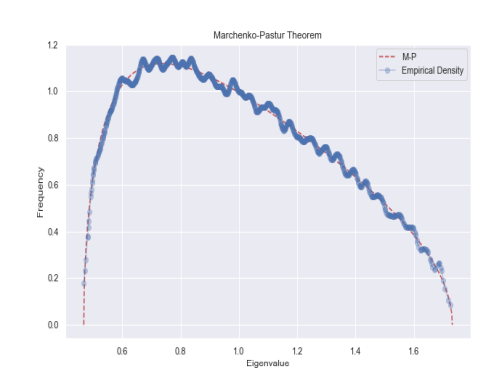
It is now appropriate to discuss the Marcenko Pastur Theorem that helps us to have homogeneous covariance matrix. The Marcenko-Pastur theorem allows us to etract signal from noise using eigenvalues of covariance matrix.
Eigenvalue and eigenvector have special meaning in financial context. Eigenvector corresponds the variance in covariance matrix while eigenvalue shows the magnitude of the eigenvector. Specifically, largest eigenvector corresponds to largest variance and the magnitude of this equals to the corresponding eigenvalue. Due to noise in the data some eigenvalues can be thought of as random and it makes sense to detect and filter these eigenvalues in order to retain signals only.
To differentiate noise and signal, we fit the Marcenko Pastur Theorem PDF to the noisy covariance. The PDF of Marcenko Pastur Theorem takes the following form (Prado, 2020):
$$
f(\lambda)= \begin{cases}\frac{T}{N} \sqrt{\left(\lambda_{t}-\lambda\right)\left(\lambda-\lambda_{-}\right)} & \text {if } \lambda \in\left[\lambda-\lambda_{-}\right] \ 0, & \text { if } \lambda \notin\left[\lambda-\lambda_{-}\right]\end{cases}
$$
where $\lambda_{+}$and $\lambda_{-}$are maximum and minimum eigenvalues.respectively. In the following code block, which is slight modification of the codes provided by Prado (2020), we will generate probability density function of Marchenko-Pastur distribution and kernel density that allows us to model a
random variable in a non-parametric approach. Then, Marchenko-Pastur distribution will be fitted to the data.
机器学习代写
统计代写|机器学习作业代写Machine Learning代考|Historical-Simulation Method
有很强的假设,如正态分布,可能是估计不准确的原因。此问题的解决方案称为历史模拟 VaR。这是一种经验方法,而不是使用参数方法,我们所做的是找到百分位数,这是方差 – 协方差方法的 Z 表等值。假设置信区间为95%, 然后5%将用于代替 Z 表值,我们需要做的就是将此百分位数乘以初始投资。
以下是历史模拟 VaR 中采取的步骤:
- 获得投资组合(或单个资产)的资产回报。
- 根据置信区间找到相应的回报百分位数。
- 将此百分位数乘以初始投资。计算95%股票收益的百分位
- (2) 估计历史模拟 VaR
- 历史模拟 VaR 方法隐含地假设历史价格变化具有相似的模式,即不存在结构性中断。这种方法的优缺点如下:
- 优点
- 没有分布假设
- 与非线性结构配合良好
- 易于计算
- 缺点
- 需要大样本
- 需要高计算能力
- 如果一家公司像成长型公司股票一样容易产生歧义,则会产生误导
统计代写|机器学习作业代写Machine Learning代考|Monte Carlo-Simulation VaR
在深入研究蒙特卡洛模拟的 VaR 估计之前,最好先简单介绍一下蒙特卡洛模拟。蒙特卡洛是一种计算机化的数学方法,用于在没有封闭解的情况下进行估计。因此,它是一种高效的数值逼近工具。蒙特卡洛依赖于给定分布的重复随机样本。
蒙特卡洛背后的逻辑由格拉瑟曼明确定义:
蒙特卡洛方法基于概率和数量之间的类比。度量的数学形式化了概率的直观概念,将事件与一组结果相关联,并将事件的概率定义为相对于一系列可能结果的体积或度量。蒙特卡洛反过来使用这个恒等式,通过将体积解释为概率来计算集合的体积。
- Glasserman (Monte Carlo Methods in Financial
Engineering, 2003, p.11)
从应用的角度来看,Monte Carlo 与历史模拟 VaR 非常相似,但它不使用历史观察。相反,它从给定分布中生成随机样本。因此,蒙特卡洛通过提供可能的结果和概率之间的联系来帮助决策者,这使其成为金融中有效且适用的工具。
数学蒙特卡罗可以定义为
:X1,X2,⋯…Xn是独立同分布的随机变量和F(X)是一个实值函数。然后,大数定律指出:
和(F(X))≈1ñ∑一世ñF(X一世)
简而言之,蒙特卡洛模拟只不过是生成随机样本并计算其平均值。在计算上,它遵循以下步骤: - 定义域
- 生成随机数
- 迭代和聚合结果
确定数学圆周率是蒙特卡洛应用程序的玩具但说明性示例。
统计代写|机器学习作业代写Machine Learning代考|Denoising
波动性无处不在,但要找出哪种波动性最有价值是一项艰巨的任务。一般来说,市场上有两种类型的信息:噪声和信号。前者只产生随机信息,但后者为我们提供了有价值的信息,投资者可以通过这些信息赚钱。为了说明,考虑市场上有两个主要参与者,一个使用噪声信息,称为噪声交易者,另一种是利用信号或内幕信息的知情交易者。噪音交易者的交易动机是由随机行为驱动的。因此,流向市场信号的信息被认为是一些噪音交易者的买入信号和其他交易者的卖出信号。
然而,知情交易者被认为是理性交易者,因为知情交易者能够评估信号,因为她知道这是私人信息。
因此,应谨慎对待信息的持续流动。简而言之,来自噪音交易者的信息可以被视为噪音,来自内部人士的信息可以被视为信号,这是重要的信息。无法区分噪音和信号的投资者可能无法获得利润和/或以适当的方式评估风险。
现在,问题变成了区分金融市场的信息流。我们如何区分噪声和信号?以及我们如何利用这些信息。
现在讨论帮助我们获得齐次协方差矩阵的 Marcenko Pastur 定理是合适的。Marcenko-Pastur 定理允许我们使用协方差矩阵的特征值从噪声中提取信号。
特征值和特征向量在金融环境中具有特殊的意义。特征向量对应于协方差矩阵中的方差,而特征值表示特征向量的大小。具体来说,最大的特征向量对应于最大的方差,其大小等于相应的特征值。由于数据中的噪声,一些特征值可以被认为是随机的,检测和过滤这些特征值以仅保留信号是有意义的。
为了区分噪声和信号,我们将 Marcenko Pastur 定理 PDF 拟合到噪声协方差。Marcenko Pastur Theorem 的 PDF 采用以下形式(Prado,2020):
F(λ)={吨ñ(λ吨−λ)(λ−λ−)如果 λ∈[λ−λ−] 0, 如果 λ∉[λ−λ−]
在哪里λ+和λ−分别是最大和最小特征值。在以下代码块中,这是对 Prado (2020) 提供的代码的轻微修改,我们将生成 Marchenko-Pastur 分布和核密度的概率密度函数,使我们能够
以非参数方法对随机变量进行建模。然后,Marchenko-Pastur 分布将适合数据。

统计代写请认准statistics-lab™. statistics-lab™为您的留学生涯保驾护航。统计代写|python代写代考
随机过程代考
在概率论概念中,随机过程是随机变量的集合。 若一随机系统的样本点是随机函数,则称此函数为样本函数,这一随机系统全部样本函数的集合是一个随机过程。 实际应用中,样本函数的一般定义在时间域或者空间域。 随机过程的实例如股票和汇率的波动、语音信号、视频信号、体温的变化,随机运动如布朗运动、随机徘徊等等。
贝叶斯方法代考
贝叶斯统计概念及数据分析表示使用概率陈述回答有关未知参数的研究问题以及统计范式。后验分布包括关于参数的先验分布,和基于观测数据提供关于参数的信息似然模型。根据选择的先验分布和似然模型,后验分布可以解析或近似,例如,马尔科夫链蒙特卡罗 (MCMC) 方法之一。贝叶斯统计概念及数据分析使用后验分布来形成模型参数的各种摘要,包括点估计,如后验平均值、中位数、百分位数和称为可信区间的区间估计。此外,所有关于模型参数的统计检验都可以表示为基于估计后验分布的概率报表。
广义线性模型代考
广义线性模型(GLM)归属统计学领域,是一种应用灵活的线性回归模型。该模型允许因变量的偏差分布有除了正态分布之外的其它分布。
statistics-lab作为专业的留学生服务机构,多年来已为美国、英国、加拿大、澳洲等留学热门地的学生提供专业的学术服务,包括但不限于Essay代写,Assignment代写,Dissertation代写,Report代写,小组作业代写,Proposal代写,Paper代写,Presentation代写,计算机作业代写,论文修改和润色,网课代做,exam代考等等。写作范围涵盖高中,本科,研究生等海外留学全阶段,辐射金融,经济学,会计学,审计学,管理学等全球99%专业科目。写作团队既有专业英语母语作者,也有海外名校硕博留学生,每位写作老师都拥有过硬的语言能力,专业的学科背景和学术写作经验。我们承诺100%原创,100%专业,100%准时,100%满意。
机器学习代写
随着AI的大潮到来,Machine Learning逐渐成为一个新的学习热点。同时与传统CS相比,Machine Learning在其他领域也有着广泛的应用,因此这门学科成为不仅折磨CS专业同学的“小恶魔”,也是折磨生物、化学、统计等其他学科留学生的“大魔王”。学习Machine learning的一大绊脚石在于使用语言众多,跨学科范围广,所以学习起来尤其困难。但是不管你在学习Machine Learning时遇到任何难题,StudyGate专业导师团队都能为你轻松解决。
多元统计分析代考
基础数据: $N$ 个样本, $P$ 个变量数的单样本,组成的横列的数据表
变量定性: 分类和顺序;变量定量:数值
数学公式的角度分为: 因变量与自变量
时间序列分析代写
随机过程,是依赖于参数的一组随机变量的全体,参数通常是时间。 随机变量是随机现象的数量表现,其时间序列是一组按照时间发生先后顺序进行排列的数据点序列。通常一组时间序列的时间间隔为一恒定值(如1秒,5分钟,12小时,7天,1年),因此时间序列可以作为离散时间数据进行分析处理。研究时间序列数据的意义在于现实中,往往需要研究某个事物其随时间发展变化的规律。这就需要通过研究该事物过去发展的历史记录,以得到其自身发展的规律。
回归分析代写
多元回归分析渐进(Multiple Regression Analysis Asymptotics)属于计量经济学领域,主要是一种数学上的统计分析方法,可以分析复杂情况下各影响因素的数学关系,在自然科学、社会和经济学等多个领域内应用广泛。
MATLAB代写
MATLAB 是一种用于技术计算的高性能语言。它将计算、可视化和编程集成在一个易于使用的环境中,其中问题和解决方案以熟悉的数学符号表示。典型用途包括:数学和计算算法开发建模、仿真和原型制作数据分析、探索和可视化科学和工程图形应用程序开发,包括图形用户界面构建MATLAB 是一个交互式系统,其基本数据元素是一个不需要维度的数组。这使您可以解决许多技术计算问题,尤其是那些具有矩阵和向量公式的问题,而只需用 C 或 Fortran 等标量非交互式语言编写程序所需的时间的一小部分。MATLAB 名称代表矩阵实验室。MATLAB 最初的编写目的是提供对由 LINPACK 和 EISPACK 项目开发的矩阵软件的轻松访问,这两个项目共同代表了矩阵计算软件的最新技术。MATLAB 经过多年的发展,得到了许多用户的投入。在大学环境中,它是数学、工程和科学入门和高级课程的标准教学工具。在工业领域,MATLAB 是高效研究、开发和分析的首选工具。MATLAB 具有一系列称为工具箱的特定于应用程序的解决方案。对于大多数 MATLAB 用户来说非常重要,工具箱允许您学习和应用专业技术。工具箱是 MATLAB 函数(M 文件)的综合集合,可扩展 MATLAB 环境以解决特定类别的问题。可用工具箱的领域包括信号处理、控制系统、神经网络、模糊逻辑、小波、仿真等。