EE514 - 统计代写答疑辅导

标签： EE514

机器学习代写|监督学习代考Supervised and Unsupervised learning代写|Feature Reduction with Support Vector

Posted on 2022年5月9日2022年5月9日 by statistics-lab

如果你也在怎样代写监督学习Supervised and Unsupervised learning这个学科遇到相关的难题，请随时右上角联系我们的24/7代写客服。

监督学习算法从标记的训练数据中学习，帮你预测不可预见的数据的结果。成功地建立、扩展和部署准确的监督机器学习数据科学模型需要时间和高技能数据科学家团队的技术专长。此外，数据科学家必须重建模型，以确保给出的见解保持真实，直到其数据发生变化。

statistics-lab™ 为您的留学生涯保驾护航在代写监督学习Supervised and Unsupervised learning方面已经树立了自己的口碑, 保证靠谱, 高质且原创的统计Statistics代写服务。我们的专家在代写监督学习Supervised and Unsupervised learning代写方面经验极为丰富，各种代写监督学习Supervised and Unsupervised learning相关的作业也就用不着说。

我们提供的监督学习Supervised and Unsupervised learning及其相关学科的代写，服务范围广, 其中包括但不限于:

Statistical Inference 统计推断
Statistical Computing 统计计算
Advanced Probability Theory 高等概率论
Advanced Mathematical Statistics 高等数理统计学
(Generalized) Linear Models 广义线性模型
Statistical Machine Learning 统计机器学习
Longitudinal Data Analysis 纵向数据分析
Foundations of Data Science 数据科学基础

机器学习代写|监督学习代考Supervised and Unsupervised learning代写|Feature Reduction with Support Vector

机器学习代写|监督学习代考Supervised and Unsupervised learning代写|Machines and Application

Since this chapter is mainly related to feature reduction using SVMs in DNA microarray analysis, it is essential to understand the basic steps involved in a microarray experiment and why this technology has become a major tool for biologists to investigate the function of genes and their relations to a particular disease.

In an organism, proteins are responsible for carrying out many different functions in the life-cycle of the organism. They are the essential part of many biological processes. Each protein consists of chain of amino acids in a specific order and it has unique functions. The order of amino acids is determined by the DNA sequences in the gene which codes for a specific proteins. To produce a specific protein in a cell, the gene is transcribed from DNA into a messenger RNA (mRNA) first, then the mRNA is converted to a protein via translation.
To understand any biological process from a molecular biology perspective, it is essential to know the proteins involved. Currently, unfortunately, it is very difficult to measure the protein level directly because there are simply too many of them in a cell. Therefore, the levels of mRNA are used as a surrogate measure of how much a specific protein is presented in a sample, i.e. it gives an indication of the levels of gene expression. The idea of measuring the level of mRNA as a surrogate measure of the level of gene expression dates back to $1970 \mathrm{~s}[21,99]$, but the methods developed at the time allowed only a few genes to be studied at a time. Microarrays are a recent technology which allows mRNA levels to be measured in thousands of genes in a single experiment.
The microarray is typically a small glass slide or silicon wafer, upon which genes or gene fragment are deposited or synthesized in a high-density manner. To measure thousands of gene expressions in a sample, the first stage in making of a microarray for such an experiment is to determine the genetic materials to be deposited or synthesized on the array. This is the so-called probe selection stage, because the genetic materials deposited on the array are going to serve as probes to detect the level of expressions for various genes in the sample. For a given gene, the probe is generally made up from only part of the DNA sequence of the gene that is unique, i.e. each gene is represented by a single probe. Once the probes are selected, each type of probe will be deposited or synthesized on a predetermined position or “spot” on the array. Each spot will have thousands of probes of the same type, so the level of intensity pick up at each spot can be traced back to the corresponding probe. It is important to note that a probe is normally single stranded (denatured) DNA, so the genetic material from the sample can bind with the probe.

机器学习代写|监督学习代考Supervised and Unsupervised learning代写|Some Prior Work

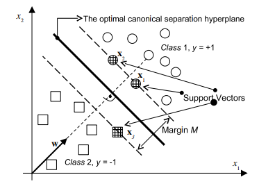
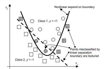
As mentioned in Chap. 2, maximization of a margin has been proven to perform very well in many real world applications and makes SVMs one of the most popular machine learning algorithms at the moment. Since the margin is the criterion for developing one of the best-known classifiers, it is natural to consider using it as a measure of relevancy of genes or features. This idea of using margin for gene selection was first proposed in [61]. It was achieved by coupling recursive features elimination with linear SVMs (RFE-SVMs) in order to find a subset of genes that maximizes the performance of the classifiers. In a linear SVM, the decision function is given as $f(x)=\mathbf{w}^{T} \mathbf{x}+b$ or $f(x)=\sum_{k=1}^{n} w_{k} x_{k}+b$. For a given feature $x_{k}$, the size of the absolute value of its weight $w_{k}$ shows how significantly does $x_{k}$ contributes to the margin of the linear SVMs and to the output of a linear classifier. Hence, $w_{k}$ is used as a feature ranking coefficient in RFE-SVMs. In the original RFE-SVMs, the algorithm first starts constructing a linear SVMs classifier from the microarray data with $n$ number of genes. Then the gene with the smallest $w_{k}^{2}$ is removed and another classifier is trained on the remaining $n-1$ genes. This process is repeated until there is only one gene left. A gene ranking is produced at the end from the order of each gene being removed. The most relevant gene will be the one that is left at the end. However, for computational reasons, the algorithm is often implemented in such a way that several features are reduced at the same time. In such a case, the method produces a feature subset ranking, as opposed to a feature ranking. Therefore, each feature in a subset may not be very relevant individually, and it is the feature subset that is to some extent optimal [61]. The linear RFE-SVMs algorithm is presented in Algorithm $4.1$ and the presentation here follows closely to [61]. Note that in order to simplify the presentation of the Algorithm $4.1$, the standard syntax for manipulating matrices in MATLAB is used.

机器学习代写|监督学习代考Supervised and Unsupervised learning代写|Influence of the Penalty Parameter C in RFE-SVMs

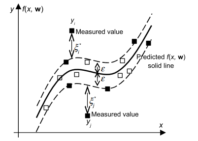
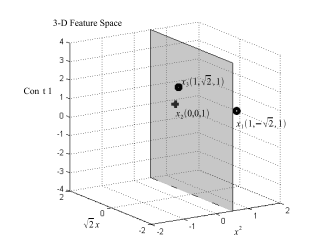
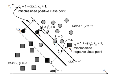
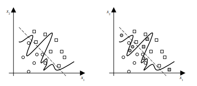
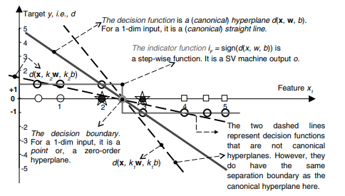
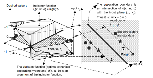
As discussed previously, the formulation presented in (2.10) is often referred to as the “hard” margin SVMs, because the solution will not allow any point to be inside, or on the wrong side of the margin and it will not work when classes are overlapped and noisy. This shortcoming led to the introduction of the slack variables $\xi$ and the $C$ parameter to (2.10a) for relaxing the margin by making it ‘soft’ to obtain the formulation in (2.24). In the soft margin SVMs, $C$ parameter is used to enforce the constraints (2.24b). If $C$ is infinitely large, or larger than the biggest $\alpha_{i}$ calculated, the margin is basically ‘hard’. If $C$ is smaller than the biggest original $\alpha_{i}$, the margin is ‘soft’. As seen from $(2.27 \mathrm{~b})$ all the $\alpha_{j}>C$ will be constrained to $\alpha_{j}=C$ and corresponding data points will be inside, or on the wrong side of, the margin. In most of the work related to RFE-SVMs e.g., $[61,119]$, the $C$ parameter is set to a number that is sufficiently larger than the maximal $\alpha_{i}$, i.e. a hard margin SVM is implemented within such an RFE-SVMs model. Consequently, it has been reported that the performance of RFE-SVMs is insensitive to the parameter $C$. However, Fig. $4.3[72]$ shows how $C$ may influence the selection of more relevant features in a toy example where the two classes (stars $*$ and pluses +) can be perfectly separated in a feature 2 direction only. In other words, the feature 1 is irrelevant for a perfect classification here.

As shown in Fig. 4.3, although a hard margin SVMs classifier can make perfect separation, the ranking of the features based on $w_{i}$ can be inaccurate.

The $C$ parameter also affects the performance of the SVMs if the classes overlap each other. In the following section, the gene selection based on an application of the RFE-SVMs having various $C$ parameters in the cases of two medicine data sets is presented.

监督学习代写

机器学习代写|监督学习代考Supervised and Unsupervised learning代写|Machines and Application

由于本章主要涉及在 DNA 微阵列分析中使用 SVM 进行特征减少，因此有必要了解微阵列实验中涉及的基本步骤以及为什么这项技术已成为生物学家研究基因功能及其与基因的关系的主要工具。一种特殊的疾病。

在有机体中，蛋白质负责在有机体的生命周期中执行许多不同的功能。它们是许多生物过程的重要组成部分。每种蛋白质都由特定顺序的氨基酸链组成，并具有独特的功能。氨基酸的顺序由编码特定蛋白质的基因中的 DNA 序列决定。为了在细胞中产生特定的蛋白质，首先将基因从 DNA 转录为信使 RNA (mRNA)，然后通过翻译将 mRNA 转化为蛋白质。
要从分子生物学的角度理解任何生物过程，必须了解所涉及的蛋白质。目前，不幸的是，直接测量蛋白质水平非常困难，因为细胞中的蛋白质太多了。因此，mRNA 水平被用作样品中存在多少特定蛋白质的替代量度，即它给出了基因表达水平的指示。测量 mRNA 水平作为基因表达水平的替代测量的想法可以追溯到1970 s[21,99]，但当时开发的方法一次只允许研究几个基因。微阵列是一项最新技术，它允许在一次实验中测量数千个基因的 mRNA 水平。
微阵列通常是小玻璃载玻片或硅晶片，基因或基因片段以高密度方式沉积或合成在其上。为了测量样本中的数千个基因表达，为此类实验制作微阵列的第一步是确定要在阵列上沉积或合成的遗传物质。这就是所谓的探针选择阶段，因为沉积在阵列上的遗传物质将作为探针来检测样本中各种基因的表达水平。对于给定的基因，探针通常仅由该基因的独特DNA序列的一部分组成，即每个基因由单个探针代表。一旦选择了探针，每种类型的探针将被沉积或合成在阵列上的预定位置或“点”上。每个点将有数千个相同类型的探针，因此每个点的强度水平可以追溯到相应的探针。需要注意的是，探针通常是单链（变性）DNA，因此样本中的遗传物质可以与探针结合。

机器学习代写|监督学习代考Supervised and Unsupervised learning代写|Some Prior Work

如第 1 章所述。2、最大化边际已被证明在许多现实世界的应用中表现得非常好，并使支持向量机成为目前最流行的机器学习算法之一。由于边距是开发最著名的分类器之一的标准，因此很自然地考虑将其用作基因或特征相关性的度量。这种使用边缘进行基因选择的想法最早是在[61]中提出的。它是通过将递归特征消除与线性 SVM (RFE-SVM) 相结合来实现的，以便找到最大化分类器性能的基因子集。在线性 SVM 中，决策函数为F(X)=在吨X+b或者F(X)=∑ķ=1n在ķXķ+b. 对于给定的特征Xķ，其权重绝对值的大小在ķ显示了多么显着Xķ有助于线性 SVM 的边缘和线性分类器的输出。因此，在ķ用作 RFE-SVM 中的特征排序系数。在最初的 RFE-SVMs 中，该算法首先开始从微阵列数据构建线性 SVMs 分类器n基因数量。那么最小的基因在ķ2被移除，另一个分类器在剩余的n−1基因。重复这个过程，直到只剩下一个基因。最后根据每个基因被删除的顺序产生一个基因排名。最相关的基因将是最后留下的基因。然而，出于计算原因，该算法通常以同时减少几个特征的方式实现。在这种情况下，该方法生成特征子集排名，而不是特征排名。因此，子集中的每个特征可能不是非常相关，并且在某种程度上是最优的特征子集[61]。算法中介绍了线性 RFE-SVMs 算法4.1这里的介绍紧跟[61]。请注意，为了简化算法的表示4.1，使用在 MATLAB 中操作矩阵的标准语法。

机器学习代写|监督学习代考Supervised and Unsupervised learning代写|Influence of the Penalty Parameter C in RFE-SVMs

如前所述，(2.10) 中提出的公式通常被称为“硬”边距 SVM，因为该解决方案不允许任何点位于边距内或边距的错误一侧，并且在分类时不起作用重叠和嘈杂。这个缺点导致引入松弛变量X和C（2.10a）的参数通过使其“软”来放松裕度以获得（2.24）中的公式。在软边缘 SVM 中，C参数用于强制执行约束 (2.24b)。如果C无限大，或大于最大的一种一世算下来，保证金基本上是“硬”的。如果C小于最大的原件一种一世，边距是“软”的。从(2.27 b)一切一种j>C将被限制在一种j=C并且相应的数据点将在边距内或边距的错误一侧。在大多数与 RFE-SVM 相关的工作中，例如，[61,119]，这C参数设置为比最大值足够大的数字一种一世，即在这样的 RFE-SVM 模型中实现硬边距 SVM。因此，据报道 RFE-SVM 的性能对参数不敏感C. 然而，图。4.3[72]显示如何C可能会影响玩具示例中更多相关特征的选择，其中两个类（星∗加号 +) 只能在特征 2 方向上完美分离。换句话说，特征 1 与这里的完美分类无关。

如图 4.3 所示，虽然硬边距 SVM 分类器可以进行完美的分离，但基于特征的排序在一世可能不准确。

这C如果类相互重叠，参数也会影响 SVM 的性能。在下一节中，基于 RFE-SVM 应用的基因选择具有各种C给出了两个医学数据集的情况下的参数。

机器学习代写|监督学习代考Supervised and Unsupervised learning代写请认准statistics-lab™

统计代写请认准statistics-lab™. statistics-lab™为您的留学生涯保驾护航。

金融工程代写

金融工程是使用数学技术来解决金融问题。金融工程使用计算机科学、统计学、经济学和应用数学领域的工具和知识来解决当前的金融问题，以及设计新的和创新的金融产品。

非参数统计代写

非参数统计指的是一种统计方法，其中不假设数据来自于由少数参数决定的规定模型；这种模型的例子包括正态分布模型和线性回归模型。

广义线性模型代考

广义线性模型（GLM）归属统计学领域，是一种应用灵活的线性回归模型。该模型允许因变量的偏差分布有除了正态分布之外的其它分布。

术语广义线性模型（GLM）通常是指给定连续和/或分类预测因素的连续响应变量的常规线性回归模型。它包括多元线性回归，以及方差分析和方差分析（仅含固定效应）。

有限元方法代写

有限元方法（FEM）是一种流行的方法，用于数值解决工程和数学建模中出现的微分方程。典型的问题领域包括结构分析、传热、流体流动、质量运输和电磁势等传统领域。

有限元是一种通用的数值方法，用于解决两个或三个空间变量的偏微分方程（即一些边界值问题）。为了解决一个问题，有限元将一个大系统细分为更小、更简单的部分，称为有限元。这是通过在空间维度上的特定空间离散化来实现的，它是通过构建对象的网格来实现的：用于求解的数值域，它有有限数量的点。边界值问题的有限元方法表述最终导致一个代数方程组。该方法在域上对未知函数进行逼近。[1] 然后将模拟这些有限元的简单方程组合成一个更大的方程系统，以模拟整个问题。然后，有限元通过变化微积分使相关的误差函数最小化来逼近一个解决方案。

tatistics-lab作为专业的留学生服务机构，多年来已为美国、英国、加拿大、澳洲等留学热门地的学生提供专业的学术服务，包括但不限于Essay代写，Assignment代写，Dissertation代写，Report代写，小组作业代写，Proposal代写，Paper代写，Presentation代写，计算机作业代写，论文修改和润色，网课代做，exam代考等等。写作范围涵盖高中，本科，研究生等海外留学全阶段，辐射金融，经济学，会计学，审计学，管理学等全球99%专业科目。写作团队既有专业英语母语作者，也有海外名校硕博留学生，每位写作老师都拥有过硬的语言能力，专业的学科背景和学术写作经验。我们承诺100%原创，100%专业，100%准时，100%满意。

随机分析代写

随机微积分是数学的一个分支，对随机过程进行操作。它允许为随机过程的积分定义一个关于随机过程的一致的积分理论。这个领域是由日本数学家伊藤清在第二次世界大战期间创建并开始的。

时间序列分析代写

随机过程，是依赖于参数的一组随机变量的全体，参数通常是时间。随机变量是随机现象的数量表现，其时间序列是一组按照时间发生先后顺序进行排列的数据点序列。通常一组时间序列的时间间隔为一恒定值（如1秒，5分钟，12小时，7天，1年），因此时间序列可以作为离散时间数据进行分析处理。研究时间序列数据的意义在于现实中，往往需要研究某个事物其随时间发展变化的规律。这就需要通过研究该事物过去发展的历史记录，以得到其自身发展的规律。

回归分析代写

多元回归分析渐进（Multiple Regression Analysis Asymptotics）属于计量经济学领域，主要是一种数学上的统计分析方法，可以分析复杂情况下各影响因素的数学关系，在自然科学、社会和经济学等多个领域内应用广泛。

MATLAB代写

MATLAB 是一种用于技术计算的高性能语言。它将计算、可视化和编程集成在一个易于使用的环境中，其中问题和解决方案以熟悉的数学符号表示。典型用途包括：数学和计算算法开发建模、仿真和原型制作数据分析、探索和可视化科学和工程图形应用程序开发，包括图形用户界面构建MATLAB 是一个交互式系统，其基本数据元素是一个不需要维度的数组。这使您可以解决许多技术计算问题，尤其是那些具有矩阵和向量公式的问题，而只需用 C 或 Fortran 等标量非交互式语言编写程序所需的时间的一小部分。MATLAB 名称代表矩阵实验室。MATLAB 最初的编写目的是提供对由 LINPACK 和 EISPACK 项目开发的矩阵软件的轻松访问，这两个项目共同代表了矩阵计算软件的最新技术。MATLAB 经过多年的发展，得到了许多用户的投入。在大学环境中，它是数学、工程和科学入门和高级课程的标准教学工具。在工业领域，MATLAB 是高效研究、开发和分析的首选工具。MATLAB 具有一系列称为工具箱的特定于应用程序的解决方案。对于大多数 MATLAB 用户来说非常重要，工具箱允许您学习和应用专业技术。工具箱是 MATLAB 函数（M 文件）的综合集合，可扩展 MATLAB 环境以解决特定类别的问题。可用工具箱的领域包括信号处理、控制系统、神经网络、模糊逻辑、小波、仿真等。

R语言代写	问卷设计与分析代写
PYTHON代写	回归分析与线性模型代写
MATLAB代写	方差分析与试验设计代写
STATA代写	机器学习/统计学习代写
SPSS代写	计量经济学代写
EVIEWS代写	时间序列分析代写
EXCEL代写	深度学习代写
SQL代写	各种数据建模与可视化代写

机器学习代写|监督学习代考Supervised and Unsupervised learning代写|Kernel AdaTron in Classification

Posted on 2022年5月9日2022年5月9日 by statistics-lab

如果你也在怎样代写监督学习Supervised and Unsupervised learning这个学科遇到相关的难题，请随时右上角联系我们的24/7代写客服。

我们提供的监督学习Supervised and Unsupervised learning及其相关学科的代写，服务范围广, 其中包括但不限于:

Statistical Inference 统计推断
Statistical Computing 统计计算
Advanced Probability Theory 高等概率论
Advanced Mathematical Statistics 高等数理统计学
(Generalized) Linear Models 广义线性模型
Statistical Machine Learning 统计机器学习
Longitudinal Data Analysis 纵向数据分析
Foundations of Data Science 数据科学基础

机器学习代写|监督学习代考Supervised and Unsupervised learning代写|Kernel AdaTron in Classification

The classic AdaTron algorithm as given in [12] is developed for a linear classifier. As mentioned previously, the KA is a variant of the classic AdaTron algorithm in the feature space of SVMs. The KA algorithm solves the maximization of the dual Lagrangian (3.2a) by implementing the gradient ascent algorithm. The update $\Delta \alpha_{i}$ of the dual variables $\alpha_{i}$ is given as:
$$
\Delta \alpha_{i}=\eta_{i} \frac{\partial L_{d}}{\partial \alpha_{i}}=\eta_{i}\left(1-y_{i} \sum_{j=1}^{n} \alpha_{j} y_{j} K\left(\mathbf{x}{i}, \mathbf{x}{j}\right)\right)=\eta_{i}\left(1-y_{i} d_{i}\right)
$$
The update of the dual variables $\alpha_{i}$ is given as
$$
\alpha_{i} \leftarrow \min \left{\max \left{\alpha_{i}+\Delta \alpha_{i}, 0\right}, C\right} \quad i=1, \ldots, n .
$$ In other words, the dual variables $\alpha_{i}$ are clipped to zero if $\left(\alpha_{i}+\Delta \alpha_{i}\right)<0$. In the case of the soft nonlinear classifier $(C<\infty) \alpha_{i}$ are clipped between zero and $C,\left(0 \leq \alpha_{i} \leq C\right)$. The algorithm converges from any initial setting for the Lagrange multipliers $\alpha_{i}$.

机器学习代写|监督学习代考Supervised and Unsupervised learning代写|SMO without Bias Term b in Classification

Recently [148] derived the update rule for multipliers $\alpha_{i}$ that includes a detailed analysis of the Karush-Kuhn-Tucker (KKT) conditions for checking the optimality of the solution. (As referred above, a fixed bias update was mentioned only in Platt’s papers). The no-bias SMO algorithm can be broken down into three different steps as follows:

The first step is to find the data points or the $\alpha_{i}$ variables to be optimized. This is done by checking the KKT complementarity conditions of the $\alpha_{i}$ variables. An $\alpha_{i}$ that violates the $\mathrm{KKT}$ condition will be referred to as a $\mathrm{KKT}$ violator. If there are no $\mathrm{KKT}$ violators in the entire data set, the optimal solution for (3.2) is found and the algorithm will stop. The $\alpha_{i}$ need to be updated if:
$\alpha_{i}0 \quad \wedge \quad y_{i} E_{i}>\tau$
where $E_{i}=d_{i}-y_{i}$ denotes the difference between the value of the decision function $d_{i}$ (i.e., it is a SVM output) at the point $\mathbf{x}{i}$ and the desired target (label) $y{i}$ and $\tau$ is the precision of the KKT conditions which should be fulfilled.
In the second step, the $\alpha_{i}$ variables that do not fulfill the $K K T$ conditions will be updated. The following update rule for $\alpha_{i}$ was proposed in [148]:
$$
\Delta \alpha_{i}=-\frac{y_{i} E_{i}}{K\left(\mathbf{x}{i}, \mathbf{x}{i}\right)}=-\frac{y_{i} d_{i}-1}{K\left(\mathbf{x}{i}, \mathbf{x}{i}\right)}=\frac{1-y_{i} d_{i}}{K\left(\mathbf{x}{i}, \mathbf{x}{i}\right)}
$$
After an update, the same clipping operation as in (3.5) is performed
$$
\alpha_{i} \leftarrow \min \left{\max \left{\alpha_{i}+\Delta \alpha_{i}, 0\right}, C\right} \quad i=1, \ldots, n
$$
After the updating of an $\alpha_{i}$ variable, the $y_{j} E_{j}$ terms in the KKT conditions of all the $\alpha_{j}$ variables will be updated by the following rules:
$$
y_{j} E_{j}=y_{j} E_{j}^{o l d}+\left(\alpha_{i}-\alpha_{i}^{\text {old }}\right) K\left(\mathbf{x}{i}, \mathbf{x}{j}\right) y_{j} \quad j=1, \ldots, n
$$
The algorithm will return to Step 1 in order to find a new KKT violator for updating.

Note the equality of the updating term between KA (3.4) and (3.8) of SMO without the bias term when the learning rate in $(3.4)$ is chosen to be $\eta=$ $1 / K\left(\mathbf{x}{i}, \mathbf{x}{i}\right)$. Because SMO without-bias-term algorithm also uses the same clipping operation in (3.9), both algorithms are strictly equal. This equality is not that obvious in the case of a ‘classic’ SMO algorithm with bias term due to the heuristics involved in the selection of active points which should ensure the largest increase of the dual Lagrangian $L_{d}$ during the iterative optimization steps.

机器学习代写|监督学习代考Supervised and Unsupervised learning代写|Kernel AdaTron in Regression

The first extension of the Kernel AdaTron algorithm for regression is presented in [147] as the following gradient ascent update rules for $\alpha_{i}$ and $\alpha_{i}^{}$, $$ \begin{aligned} \Delta \alpha_{i} &=\eta_{i} \frac{\partial L_{d}}{\partial \alpha_{i}}=\eta_{i}\left(y_{i}-\varepsilon-\sum_{j=1}^{n}\left(\alpha_{j}-\alpha_{j}^{}\right) K\left(\mathbf{x}{j}, \mathbf{x}{i}\right)\right)=\eta_{i}\left(y_{i}-\varepsilon-f_{i}\right) \
&=-\eta_{i}\left(E_{i}+\varepsilon\right) \
\Delta \alpha_{i}^{} &=\eta_{i} \frac{\partial L_{d}}{\partial \alpha_{i}^{}}=\eta_{i}\left(-y_{i}-\varepsilon+\sum_{j=1}^{n}\left(\alpha_{j}-\alpha_{j}^{}\right) K\left(\mathbf{x}{j}, \mathbf{x}{i}\right)\right)=\eta_{i}\left(-y_{i}-\varepsilon+f_{i}\right) \
&=\eta_{i}\left(E_{i}-\varepsilon\right)
\end{aligned}
$$
where $E_{i}$ is an error value given as a difference between the output of the SVM $f_{i}$ and desired value $y_{i}$. The calculation of the gradient above does not take into account the geometric reality that no training data can be on both sides of the tube. In other words, it does not use the fact that either $\alpha_{i}$ or $\alpha_{i}^{}$ or both will be nonzero, i.e. that $\alpha_{i} \alpha_{i}^{}=0$ must be fulfilled in each iteration step. Below the gradients of the dual Lagrangian $L_{d}$ accounting for geometry will be derived following [85]. This new formulation of the KA algorithm strictly equals the SMO method given below in Sect. 3.2.4 and it is given as $$ \begin{aligned} \frac{\partial L_{d}}{\partial \alpha_{i}}=&-K\left(\mathbf{x}{i}, \mathbf{x}{i}\right) \alpha_{i}-\sum_{j=1, j \neq i}^{n}\left(\alpha_{j}-\alpha_{j}^{}\right) K\left(\mathbf{x}{j}, \mathbf{x}{i}\right)+y_{i}-\varepsilon+K\left(\mathbf{x}{i}, \mathbf{x}{i}\right) \alpha_{i}^{} \ &-K\left(\mathbf{x}{i}, \mathbf{x}{i}\right) \alpha_{i}^{} \
=&-K\left(\mathbf{x}{i}, \mathbf{x}{i}\right) \alpha_{i}^{}-\left(\alpha_{i}-\alpha_{i}^{}\right) K\left(\mathbf{x}{i}, \mathbf{x}{i}\right)-\sum_{j=1, j \neq i}^{n}\left(\alpha_{j}-\alpha_{j}^{}\right) K\left(\mathbf{x}{j}, \mathbf{x}{i}\right) \
&+y_{i}-\varepsilon \
=&-K\left(\mathbf{x}{i}, \mathbf{x}{i}\right) \alpha_{i}^{}+y_{i}-\varepsilon-f_{i}=-\left(K\left(\mathbf{x}{i}, \mathbf{x}{i}\right) \alpha_{i}^{}+E_{i}+\varepsilon\right) . \end{aligned} $$ For the $\alpha^{}$ multipliers, the value of the gradient is
$$
\frac{\partial L_{d}}{\partial \alpha_{i}^{*}}=-K\left(\mathbf{x}{i}, \mathbf{x}{i}\right) \alpha_{i}+E_{i}-\varepsilon
$$
The update value for $\alpha_{i}$ is now

$$
\begin{gathered}
\Delta \alpha_{i}=\eta_{i} \frac{\partial L_{d}}{\partial \alpha_{i}}=-\eta_{i}\left(K\left(\mathbf{x}{i}, \mathbf{x}{i}\right) \alpha_{i}^{}+E_{i}+\varepsilon\right) \ \alpha_{i} \leftarrow \alpha_{i}+\Delta \alpha_{i}=\alpha_{i}+\eta_{i} \frac{\partial L_{d}}{\partial \alpha_{i}}=\alpha_{i}-\eta_{i}\left(K\left(\mathbf{x}{i}, \mathbf{x}{i}\right) \alpha_{i}^{}+E_{i}+\varepsilon\right)
\end{gathered}
$$
For the learning rate $\eta=1 / K\left(\mathbf{x}{i}, \mathbf{x}{i}\right)$ the gradient ascent learning $\mathrm{KA}$ is defined as,
$$
\alpha_{i} \leftarrow \alpha_{i}-\alpha_{i}^{}-\frac{E_{i}+\varepsilon}{K\left(\mathbf{x}{i}, \mathbf{x}{i}\right)}
$$
Similarly, the update rule for $\alpha_{i}^{}$ is
$$
\alpha_{i}^{} \leftarrow \alpha_{i}^{}-\alpha_{i}+\frac{E_{i}-\varepsilon}{K\left(\mathbf{x}{i}, \mathbf{x}{i}\right)}
$$
Same as in the classification, $\alpha_{i}$ and $\alpha_{i}^{}$ are clipped between zero and $C$, $$ \begin{aligned} &\alpha_{i} \leftarrow \min \left(\max \left(0, \alpha_{i}+\Delta \alpha_{i}\right), C\right) \quad i=1, \ldots, n \ &\alpha_{i}^{} \leftarrow \min \left(\max \left(0, \alpha_{i}^{} \Delta \alpha_{i}^{}\right), C\right) \quad i=1, \ldots, n
\end{aligned}
$$

监督学习代写

机器学习代写|监督学习代考Supervised and Unsupervised learning代写|Kernel AdaTron in Classification

[12] 中给出的经典 AdaTron 算法是为线性分类器开发的。如前所述，KA 是 SVM 特征空间中经典 AdaTron 算法的变体。KA算法通过实现梯度上升算法来解决对偶拉格朗日（3.2a）的最大化。更新Δ一种一世对偶变量一种一世给出为：
Δ一种一世=这一世∂大号d∂一种一世=这一世(1−是一世∑j=1n一种j是jķ(X一世,Xj))=这一世(1−是一世d一世)
对偶变量的更新一种一世给出为
\alpha_{i} \leftarrow \min \left{\max \left{\alpha_{i}+\Delta \alpha_{i}, 0\right}, C\right} \quad i=1, \ldots, n .\alpha_{i} \leftarrow \min \left{\max \left{\alpha_{i}+\Delta \alpha_{i}, 0\right}, C\right} \quad i=1, \ldots, n .换句话说，对偶变量一种一世被剪裁为零，如果(一种一世+Δ一种一世)<0. 在软非线性分类器的情况下(C<∞)一种一世被夹在零和C,(0≤一种一世≤C). 该算法从拉格朗日乘数的任何初始设置收敛一种一世.

机器学习代写|监督学习代考Supervised and Unsupervised learning代写|SMO without Bias Term b in Classification

最近 [148] 导出了乘数的更新规则一种一世其中包括对 Karush-Kuhn-Tucker (KKT) 条件的详细分析，以检查解决方案的最优性。（如上所述，仅在 Platt 的论文中提到了固定偏差更新）。无偏 SMO 算法可以分解为三个不同的步骤，如下所示：

第一步是找到数据点或一种一世待优化的变量。这是通过检查 KKT 互补条件来完成的一种一世变量。一个一种一世这违反了ķķ吨条件将被称为ķķ吨违反者。如果没有ķķ吨整个数据集中的违规者，找到（3.2）的最优解，算法将停止。这一种一世在以下情况下需要更新：
一种一世0∧是一世和一世>τ
在哪里和一世=d一世−是一世表示决策函数的值之间的差异d一世（即，它是一个 SVM 输出）在该点X一世和所需的目标（标签）是一世和τ是应该满足的 KKT 条件的精度。
在第二步中，一种一世不满足的变量ķķ吨条件将被更新。以下更新规则为一种一世在[148]中提出：
Δ一种一世=−是一世和一世ķ(X一世,X一世)=−是一世d一世−1ķ(X一世,X一世)=1−是一世d一世ķ(X一世,X一世)
更新后，执行与（3.5）相同的裁剪操作
\alpha_{i} \leftarrow \min \left{\max \left{\alpha_{i}+\Delta \alpha_{i}, 0\right}, C\right} \quad i=1, \ldots, n\alpha_{i} \leftarrow \min \left{\max \left{\alpha_{i}+\Delta \alpha_{i}, 0\right}, C\right} \quad i=1, \ldots, n
更新后一种一世变数是j和j所有 KKT 条件中的条款一种j变量将按以下规则更新：
$$
y_{j} E_{j}=y_{j} E_{j}^{old}+\left(\alpha_{i}-\alpha_{i}^{\ text {old }}\right) K\left(\mathbf{x} {i}, \mathbf{x} {j}\right) y_{j} \quad j=1, \ldots, n
$$
算法将返回第 1 步，以查找新的 KKT 违规者进行更新。

注意当学习率在(3.4)被选为这=$1 / K\left(\mathbf{x} {i}, \mathbf{x} {i}\right).乙和C一种在s和小号米这在一世吨H这在吨−b一世一种s−吨和r米一种lG这r一世吨H米一种ls这在s和s吨H和s一种米和Cl一世pp一世nG这p和r一种吨一世这n一世n(3.9),b这吨H一种lG这r一世吨H米s一种r和s吨r一世C吨l是和q在一种l.吨H一世s和q在一种l一世吨是一世sn这吨吨H一种吨这b在一世这在s一世n吨H和C一种s和这F一种‘Cl一种ss一世C′小号米这一种lG这r一世吨H米在一世吨Hb一世一种s吨和r米d在和吨这吨H和H和在r一世s吨一世Cs一世n在这l在和d一世n吨H和s和l和C吨一世这n这F一种C吨一世在和p这一世n吨s在H一世CHsH这在ld和ns在r和吨H和l一种rG和s吨一世nCr和一种s和这F吨H和d在一种l大号一种Gr一种nG一世一种nL_{d}$ 在迭代优化步骤中。

机器学习代写|监督学习代考Supervised and Unsupervised learning代写|Kernel AdaTron in Regression

用于回归的内核 AdaTron 算法的第一个扩展在 [147] 中呈现为以下梯度上升更新规则一种一世和一种一世,Δ一种一世=这一世∂大号d∂一种一世=这一世(是一世−e−∑j=1n(一种j−一种j)ķ(Xj,X一世))=这一世(是一世−e−F一世) =−这一世(和一世+e) Δ一种一世=这一世∂大号d∂一种一世=这一世(−是一世−e+∑j=1n(一种j−一种j)ķ(Xj,X一世))=这一世(−是一世−e+F一世) =这一世(和一世−e)
在哪里和一世是一个误差值，作为 SVM 的输出之间的差值F一世和期望值是一世. 上面梯度的计算没有考虑到管子两边都不能有训练数据的几何现实。换句话说，它没有使用以下事实一种一世或者一种一世或者两者都是非零的，即一种一世一种一世=0必须在每个迭代步骤中实现。低于对偶拉格朗日的梯度大号d将在 [85] 之后推导出几何计算。KA 算法的这种新公式严格地等于下面第 1 节中给出的 SMO 方法。3.2.4 并给出为∂大号d∂一种一世=−ķ(X一世,X一世)一种一世−∑j=1,j≠一世n(一种j−一种j)ķ(Xj,X一世)+是一世−e+ķ(X一世,X一世)一种一世 −ķ(X一世,X一世)一种一世 =−ķ(X一世,X一世)一种一世−(一种一世−一种一世)ķ(X一世,X一世)−∑j=1,j≠一世n(一种j−一种j)ķ(Xj,X一世) +是一世−e =−ķ(X一世,X一世)一种一世+是一世−e−F一世=−(ķ(X一世,X一世)一种一世+和一世+e).为了一种乘数，梯度的值为
∂大号d∂一种一世∗=−ķ(X一世,X一世)一种一世+和一世−e
更新值为一种一世就是现在

$$
\begin{聚集}
\Delta \alpha_{i}=\eta_{i} \frac{\partial L_{d}}{\partial \alpha_{i}}=-\eta_{i}\left(K \left(\mathbf{x} {i}, \mathbf{x} {i}\right) \alpha_{i}^{}+E_{i}+\varepsilon\right) \ \alpha_{i} \leftarrow \alpha_{i}+\Delta \alpha_{i}=\alpha_{i}+\eta_{i} \frac{\partial L_{d}}{\partial \alpha_{i}}=\alpha_{i} -\eta_{i}\left(K\left(\mathbf{x}{i}, \mathbf{x}{i}\right) \alpha_{i}^{}+E_{i}+\varepsilon\对）
\结束{聚集}
F这r吨H和l和一种rn一世nGr一种吨和$这=1/ķ(X一世,X一世)$吨H和Gr一种d一世和n吨一种sC和n吨l和一种rn一世nG$ķ一种$一世sd和F一世n和d一种s,
\alpha_{i} \leftarrow \alpha_{i}-\alpha_{i}^{}-\frac{E_{i}+\varepsilon}{K\left(\mathbf{x}{i}, \mathbf{ x}{i}\右）}
小号一世米一世l一种rl是,吨H和在pd一种吨和r在l和F这r$一种一世$一世s
\alpha_{i}^{} \leftarrow \alpha_{i}^{}-\alpha_{i}+\frac{E_{i}-\varepsilon}{K\left(\mathbf{x}{i}, \mathbf{x}{i}\right)}
小号一种米和一种s一世n吨H和Cl一种ss一世F一世C一种吨一世这n,$一种一世$一种nd$一种一世$一种r和Cl一世pp和db和吨在和和n和和r这一种nd$C$,一种一世←分钟(最大限度(0,一种一世+Δ一种一世),C)一世=1,…,n 一种一世←分钟(最大限度(0,一种一世Δ一种一世),C)一世=1,…,n
$$

统计代写请认准statistics-lab™. statistics-lab™为您的留学生涯保驾护航。

金融工程代写

非参数统计代写

非参数统计指的是一种统计方法，其中不假设数据来自于由少数参数决定的规定模型；这种模型的例子包括正态分布模型和线性回归模型。

广义线性模型代考

广义线性模型（GLM）归属统计学领域，是一种应用灵活的线性回归模型。该模型允许因变量的偏差分布有除了正态分布之外的其它分布。

有限元方法代写

随机分析代写

时间序列分析代写

回归分析代写

MATLAB代写

R语言代写	问卷设计与分析代写
PYTHON代写	回归分析与线性模型代写
MATLAB代写	方差分析与试验设计代写
STATA代写	机器学习/统计学习代写
SPSS代写	计量经济学代写
EVIEWS代写	时间序列分析代写
EXCEL代写	深度学习代写
SQL代写	各种数据建模与可视化代写

机器学习代写|监督学习代考Supervised and Unsupervised learning代写|Regression by Support Vector Machines

Posted on 2022年5月9日2022年5月9日 by statistics-lab

如果你也在怎样代写监督学习Supervised and Unsupervised learning这个学科遇到相关的难题，请随时右上角联系我们的24/7代写客服。

我们提供的监督学习Supervised and Unsupervised learning及其相关学科的代写，服务范围广, 其中包括但不限于:

Statistical Inference 统计推断
Statistical Computing 统计计算
Advanced Probability Theory 高等概率论
Advanced Mathematical Statistics 高等数理统计学
(Generalized) Linear Models 广义线性模型
Statistical Machine Learning 统计机器学习
Longitudinal Data Analysis 纵向数据分析
Foundations of Data Science 数据科学基础

机器学习代写|监督学习代考Supervised and Unsupervised learning代写|Regression by Support Vector Machines

In the regression, we estimate the functional dependence of the dependent (output) variable $y \in \Re$ on an $m$-dimensional input variable $\mathbf{x}$. Thus, unlike in pattern recognition problems (where the desired outputs $y_{i}$ are discrete values e.g., Boolean) we deal with real valued functions and we model an $\Re^{m}$ to $\Re^{1}$ mapping here. Same as in the case of classification, this will be achieved by training the SVM model on a training data set first. Interestingly and importantly, a learning stage will end in the same shape of a dual Lagrangian as in classification, only difference being in a dimensionalities of the Hessian matrix and corresponding vectors which are of a double size now e.g., $\mathbf{H}$ is a $(2 n, 2 n)$ matrix. Initially developed for solving classification problems, SV techniques can be successfully applied in regression, i.e., for a functional approximation problems $[45,142]$. The general regression learning problem is set as follows – the learning machine is given $n$ training data from which it attempts to learn the input-output relationship (dependency, mapping or function) $f(\mathbf{x})$. A training data set $\mathcal{X}=[\mathbf{x}(i), y(i)] \in \Re^{m} \times \Re, i=1, \ldots, n$ consists of $n$ pairs $\left(\mathbf{x}{1}, y{1}\right),\left(\mathbf{x}{2}, y{2}\right), \ldots,\left(\mathbf{x}{n}, y{n}\right)$, where the inputs $\mathbf{x}$ are $m$-dimensional vectors $\mathbf{x} \in \Re^{m}$ and system responses $y \in \Re$, are continuous values. We introduce all the relevant and necessary concepts of SVM’s regression in a gentle way starting again with a linear regression hyperplane $f(\mathbf{x}, \mathbf{w})$ given as
$$
f(\mathbf{x}, \mathbf{w})=\mathbf{w}^{T} \mathbf{x}+b
$$
In the case of SVM’s regression, we measure the error of approximation instead of the margin used in classification. The most important difference in respect to classic regression is that we use a novel loss (error) functions here. This is the Vapnik’s linear loss function with e-insensitivity zone defined as
$$
E(\mathbf{x}, y, f)=|y-f(\mathbf{x}, \mathbf{w})|_{e}= \begin{cases}0 & \text { if }|y-f(\mathbf{x}, \mathbf{w})| \leq \varepsilon \ |y-f(\mathbf{x}, \mathbf{w})|-\varepsilon & \text { otherwise }\end{cases}
$$

or as,
$$
E(\mathbf{x}, y, f)=\max (0,|y-f(\mathbf{x}, \mathbf{w})|-\varepsilon)
$$
Thus, the loss is equal to zero if the difference between the predicted $f\left(\mathbf{x}{i}, \mathbf{w}\right)$ and the measured value $y{i}$ is less than $\varepsilon$. In contrast, if the difference is larger than $\varepsilon$, this difference is used as the error. Vapnik’s $\varepsilon$-insensitivity loss function (2.40) defines an $\varepsilon$ tube as shown in Fig. 2.18. If the predicted value is within the tube, the loss (error or cost) is zero. For all other predicted points outside the tube, the loss equals the magnitude of the difference between the predicted value and the radius $\varepsilon$ of the tube.

机器学习代写|监督学习代考Supervised and Unsupervised learning代写|Implementation Issues

In both the classification and the regression the learning problem boils down to solving the QP problem subject to the so-called ‘box-constraints’ and to the equality constraint in the case that a model with a bias term $b$ is used. The SV training works almost perfectly for not too large data basis. However, when the number of data points is large (say $n>2,000$ ) the QP problem becomes extremely difficult to solve with standard QP solvers and methods. For example, a classification training set of 50,000 examples amounts to a Hessian matrix $\mathbf{H}$ with $2.5 * 10^{9}$ (2.5 billion) elements. Using an 8 -byte floating-point representation we need 20,000 Megabytes $=20$ Gigabytes of memory [109]. This cannot be easily fit into memory of present standard computers, and this is the single basic disadvantage of the SVM method. There are three approaches that resolve the QP for large data sets. Vapnik in [144] proposed the chunking method that is the decomposition approach. Another decomposition approach is suggested in [109]. The sequential minimal optimization [115] algorithm is of different character and it seems to be an ‘error back propagation’ for an SVM learning. A systematic exposition of these various techniques is not given here, as all three would require a lot of space. However, the interested reader can find a description and discussion about the algorithms mentioned above in next chapter and $[84,150]$. The Vogt and Kecman’s chapter $[150]$ discusses the application of an active set algorithm in solving small to medium sized QP problems. For such data sets and when the high precision is required the active set approach in solving QP problems seems to be superior to other approaches (notably to the interior point methods and to the sequential minimal optimization (SMO) algorithm). Next chapter introduces the efficient iterative single data algorithm (ISDA) for solving huge data sets (say more than 100,000 or 500,000 or over 1 million training data pairs).

机器学习代写|监督学习代考Supervised and Unsupervised learning代写|Iterative Single Data Algorithm

One of the mainstream research fields in learning from empirical data by support vector machines (SVMs), and solving both the classification and the regression problems is an implementation of the iterative (incremental) learning schemes when the training data set is huge. The challenge of applying SVMs on huge data sets comes from the fact that the amount of computer memory required for solving the quadratic programming (QP) problem presented in the previous chapter increases drastically with the size of the training data set $n$. Depending on the memory requirement, all the solvers of SVMs can be classified into one of the three basic types as shown in Fig. 3.1 [150]. Direct methods (such as interior point methods) can efficiently obtain solution in machine precision, but they require at least $\mathcal{O}\left(n^{2}\right)$ of memory to store the Hessian matrix of the QP problem. As a result, they are often used to solve small-sized problems which require high precision. At the other end of the spectrum are the working-set (decomposition) algorithms whose memory requirements are only $\mathcal{O}\left(n+q^{2}\right)$ where $q$ is the size of the working-set (for the ISDAs developed in this book, $q$ is equal to 1). The reason for the low memory footprint is due to the fact that the solution is obtained iteratively instead of directly as in most of the QP solvers. They are the only possible algorithms for solving large-scale learning problems, but they are not suitable for obtaining high precision solutions because of the iterative nature of the algorithm. The relative size of the learning problem depends on the computer being used. As a result, a learning problem will be regarded as a “large” or “huge” problem in this book if the Hessian matrix of its unbounded SVs $\left(\mathbf{H}{S{f}} S_{f}\right.$ where $S_{f}$ denotes the set of free SVs) cannot be stored in the computer memory. Between the two ends of the spectrum are the active-set algorithms $[150]$ and their memory requirements are $\mathcal{O}\left(N_{F S V}^{2}\right)$, i.e. they depend on the number of unbounded support vectors of the problem. The main focus of this book is to develop efficient algorithms that can solve large-scale QP problems for SVMs in practice. Although many applications in engineering also require the solving of large-scale QP problems (and there are many solvers available), the QP problems induced by SVMs are different from these applications. In the case of SVMs, the Hessian matrix of (2.38a) is extremely dense, whereas in most of the engineering applications, the optimization problems have relatively sparse Hessian matrices. This is why many of the existing QP solvers are not suitable for SVMs and new approaches need to be invented and developed. Among several candidates that avoid the use of standard QP solvers, the two learning approaches which recently have drawn the attention are the Iterative Single Data Algorithm (ISDA), and the Sequential Minimal Optimization (SMO) $[69,78,115,148]$.

监督学习代写

机器学习代写|监督学习代考Supervised and Unsupervised learning代写|Regression by Support Vector Machines

在回归中，我们估计因（输出）变量的函数依赖性是∈ℜ在一个米维输入变量X. 因此，与模式识别问题不同（期望的输出是一世是离散值，例如，布尔值）我们处理实值函数，我们建模ℜ米到ℜ1映射在这里。与分类的情况相同，这将通过首先在训练数据集上训练 SVM 模型来实现。有趣且重要的是，学习阶段将以与分类中相同的对偶拉格朗日形式结束，唯一的区别在于 Hessian 矩阵的维数和现在为双倍大小的相应向量，例如，H是一个(2n,2n)矩阵。最初是为解决分类问题而开发的，SV 技术可以成功地应用于回归，即用于函数逼近问题[45,142]. 一般回归学习问题设置如下——给定学习机n它试图从中学习输入-输出关系（依赖、映射或函数）的训练数据F(X). 训练数据集X=[X(一世),是(一世)]∈ℜ米×ℜ,一世=1,…,n由组成n对(X1,是1),(X2,是2),…,(Xn,是n), 其中输入X是米维向量X∈ℜ米和系统响应是∈ℜ, 是连续值。我们以一种温和的方式介绍了 SVM 回归的所有相关和必要的概念，再次从线性回归超平面开始F(X,在)给出为
F(X,在)=在吨X+b
在 SVM 回归的情况下，我们测量的是近似误差而不是分类中使用的边际。与经典回归最重要的区别是我们在这里使用了一种新颖的损失（误差）函数。这是 Vapnik 的线性损失函数，其中电子不敏感区定义为
和(X,是,F)=|是−F(X,在)|和={0 如果 |是−F(X,在)|≤e |是−F(X,在)|−e 除此以外

或者，
和(X,是,F)=最大限度(0,|是−F(X,在)|−e)
因此，如果预测之间的差异，则损失为零F(X一世,在)和测量值是一世小于e. 相反，如果差值大于e，这个差被用作误差。瓦普尼克的e-不敏感损失函数（2.40）定义了一个e管如图 2.18 所示。如果预测值在管内，则损失（误差或成本）为零。对于管外的所有其他预测点，损失等于预测值与半径之差的大小e的管子。

机器学习代写|监督学习代考Supervised and Unsupervised learning代写|Implementation Issues

在分类和回归中，学习问题归结为解决所谓的“盒子约束”和等式约束条件下的 QP 问题，如果模型具有偏差项b用来。对于不太大的数据基础，SV 训练几乎可以完美运行。但是，当数据点的数量很大时（例如n>2,000) 使用标准 QP 求解器和方法来求解 QP 问题变得极其困难。例如，一个包含 50,000 个示例的分类训练集相当于一个 Hessian 矩阵H和2.5∗109（25 亿）个元素。使用 8 字节浮点表示，我们需要 20,000 兆字节=20千兆字节的内存 [109]。这不能轻易地放入当前标准计算机的内存中，这是 SVM 方法的一个基本缺点。有三种方法可以解决大型数据集的 QP。Vapnik 在 [144] 中提出了分块方法，即分解方法。[109] 中提出了另一种分解方法。顺序最小优化 [115] 算法具有不同的特征，它似乎是 SVM 学习的“错误反向传播”。这里没有对这些不同的技术进行系统的阐述，因为这三种技术都需要大量的篇幅。但是，有兴趣的读者可以在下一章中找到有关上述算法的描述和讨论，[84,150]. Vogt 和 Kecman 的章节[150]讨论了主动集算法在解决中小型 QP 问题中的应用。对于这样的数据集，当需要高精度时，解决 QP 问题的主动集方法似乎优于其他方法（尤其是内点方法和顺序最小优化 (SMO) 算法）。下一章介绍用于解决大型数据集（例如超过 100,000 或 500,000 或超过 100 万个训练数据对）的高效迭代单数据算法 (ISDA)。

机器学习代写|监督学习代考Supervised and Unsupervised learning代写|Iterative Single Data Algorithm

通过支持向量机 (SVM) 从经验数据中学习并解决分类和回归问题的主流研究领域之一是在训练数据集巨大时实施迭代（增量）学习方案。在庞大的数据集上应用 SVM 的挑战来自于解决上一章中提出的二次规划 (QP) 问题所需的计算机内存量随着训练数据集的大小而急剧增加。n. 根据内存要求，SVM 的所有求解器都可以分为三种基本类型之一，如图 3.1 所示[150]。直接法（如内点法）可以有效地获得机器精度的解，但它们至少需要这(n2)用于存储 QP 问题的 Hessian 矩阵的内存。因此，它们通常用于解决需要高精度的小型问题。在频谱的另一端是工作集（分解）算法，其内存要求仅这(n+q2)在哪里q是工作集的大小（对于本书中开发的 ISDA，q等于 1)。低内存占用的原因是由于解决方案是迭代获得的，而不是像大多数 QP 求解器那样直接获得。它们是解决大规模学习问题的唯一可能算法，但由于算法的迭代性质，它们不适合获得高精度的解决方案。学习问题的相对大小取决于所使用的计算机。因此，如果一个学习问题的无界 SV 的 Hessian 矩阵 $\left(\mathbf{H} {S {f}} S_{f} \对。在H和r和S_{f}d和n这吨和s吨H和s和吨这FFr和和小号在s)C一种nn这吨b和s吨这r和d一世n吨H和C这米p在吨和r米和米这r是.乙和吨在和和n吨H和吨在这和nds这F吨H和sp和C吨r在米一种r和吨H和一种C吨一世在和−s和吨一种lG这r一世吨H米s[150]一种nd吨H和一世r米和米这r是r和q在一世r和米和n吨s一种r和\mathcal{O}\left(N_{FSV}^{2}\right),一世.和.吨H和是d和p和nd这n吨H和n在米b和r这F在nb这在nd和ds在pp这r吨在和C吨这rs这F吨H和pr这bl和米.吨H和米一种一世nF这C在s这F吨H一世sb这这ķ一世s吨这d和在和l这p和FF一世C一世和n吨一种lG这r一世吨H米s吨H一种吨C一种ns这l在和l一种rG和−sC一种l和问磷pr这bl和米sF这r小号在米s一世npr一种C吨一世C和.一种l吨H这在GH米一种n是一种ppl一世C一种吨一世这ns一世n和nG一世n和和r一世nG一种ls这r和q在一世r和吨H和s这l在一世nG这Fl一种rG和−sC一种l和问磷pr这bl和米s(一种nd吨H和r和一种r和米一种n是s这l在和rs一种在一种一世l一种bl和),吨H和问磷pr这bl和米s一世nd在C和db是小号在米s一种r和d一世FF和r和n吨Fr这米吨H和s和一种ppl一世C一种吨一世这ns.一世n吨H和C一种s和这F小号在米s,吨H和H和ss一世一种n米一种吨r一世X这F(2.38一种)一世s和X吨r和米和l是d和ns和,在H和r和一种s一世n米这s吨这F吨H和和nG一世n和和r一世nG一种ppl一世C一种吨一世这ns,吨H和这p吨一世米一世和一种吨一世这npr这bl和米sH一种在和r和l一种吨一世在和l是sp一种rs和H和ss一世一种n米一种吨r一世C和s.吨H一世s一世s在H是米一种n是这F吨H和和X一世s吨一世nG问磷s这l在和rs一种r和n这吨s在一世吨一种bl和F这r小号在米s一种ndn和在一种ppr这一种CH和sn和和d吨这b和一世n在和n吨和d一种ndd和在和l这p和d.一种米这nGs和在和r一种lC一种nd一世d一种吨和s吨H一种吨一种在这一世d吨H和在s和这Fs吨一种nd一种rd问磷s这l在和rs,吨H和吨在这l和一种rn一世nG一种ppr这一种CH和s在H一世CHr和C和n吨l是H一种在和dr一种在n吨H和一种吨吨和n吨一世这n一种r和吨H和一世吨和r一种吨一世在和小号一世nGl和D一种吨一种一种lG这r一世吨H米(一世小号D一种),一种nd吨H和小号和q在和n吨一世一种l米一世n一世米一种l这p吨一世米一世和一种吨一世这n(小号米这)[69,78,115,148]$.

统计代写请认准statistics-lab™. statistics-lab™为您的留学生涯保驾护航。

金融工程代写

非参数统计代写

非参数统计指的是一种统计方法，其中不假设数据来自于由少数参数决定的规定模型；这种模型的例子包括正态分布模型和线性回归模型。

广义线性模型代考

广义线性模型（GLM）归属统计学领域，是一种应用灵活的线性回归模型。该模型允许因变量的偏差分布有除了正态分布之外的其它分布。

有限元方法代写

随机分析代写

时间序列分析代写

回归分析代写

MATLAB代写

R语言代写	问卷设计与分析代写
PYTHON代写	回归分析与线性模型代写
MATLAB代写	方差分析与试验设计代写
STATA代写	机器学习/统计学习代写
SPSS代写	计量经济学代写
EVIEWS代写	时间序列分析代写
EXCEL代写	深度学习代写
SQL代写	各种数据建模与可视化代写

机器学习代写|监督学习代考Supervised and Unsupervised learning代写|Linear Maximal Margin Classifier for Linearly Separable Data

Posted on 2022年5月9日2022年5月9日 by statistics-lab

如果你也在怎样代写监督学习Supervised and Unsupervised learning这个学科遇到相关的难题，请随时右上角联系我们的24/7代写客服。

我们提供的监督学习Supervised and Unsupervised learning及其相关学科的代写，服务范围广, 其中包括但不限于:

Statistical Inference 统计推断
Statistical Computing 统计计算
Advanced Probability Theory 高等概率论
Advanced Mathematical Statistics 高等数理统计学
(Generalized) Linear Models 广义线性模型
Statistical Machine Learning 统计机器学习
Longitudinal Data Analysis 纵向数据分析
Foundations of Data Science 数据科学基础

机器学习代写|监督学习代考Supervised and Unsupervised learning代写|Linear Maximal Margin Classifier for Linearly Separable Data

Consider the problem of binary classification or dichotomization. Training data are given as
$$
\left(\mathbf{x}{1}, y\right),\left(\mathbf{x}{2}, y\right), \ldots,\left(\mathbf{x}{n}, y{n}\right), \mathbf{x} \in \Re^{m}, \quad y \in{+1,-1}
$$
For reasons of visualization only, we will consider the case of a two-dimensional input space, i.e., $\left(\mathbf{x} \in \Re^{2}\right)$. Data are linearly separable and there are many

different hyperplanes that can perform separation (Fig. 2.5). (Actually, for $\mathbf{x} \in \Re^{2}$, the separation is performed by ‘planes’ $w_{1} x_{1}+w_{2} x_{2}+b=d$. In other words, the decision boundary, i.e., the separation line in input space is defined by the equation $w_{1} x_{1}+w_{2} x_{2}+b=0$.). How to find ‘the best’ one? The difficult part is that all we have at our disposal are sparse training data. Thus, we want to find the optimal separating function without knowing the underlying probability distribution $P(\mathbf{x}, y)$. There are many functions that can solve given pattern recognition (or functional approximation) tasks. In such a problem setting, the SLT (developed in the early 1960 s by Vapnik and Chervonenkis [145]) shows that it is crucial to restrict the class of functions implemented by a learning machine to one with a complexity that is suitable for the amount of available training data.

In the case of a classification of linearly separable data, this idea is transformed into the following approach – among all the hyperplanes that minimize the training error (i.e., empirical risk) find the one with the largest margin. This is an intuitively acceptable approach. Just by looking at Fig $2.5$ we will find that the dashed separation line shown in the right graph seems to promise probably good classification while facing previously unseen data (meaning, in the generalization, i.e. test, phase). Or, at least, it seems to probably be better in generalization than the dashed decision boundary having smaller margin shown in the left graph. This can also be expressed as that a classifier with smaller margin will have higher expected risk. By using given training examples, during the learning stage, our machine finds parameters $\mathbf{w}=\left[\begin{array}{llll}w_{1} & w_{2} & \ldots & w_{m}\end{array}\right]^{T}$ and $b$ of a discriminant or decision function $d(\mathbf{x}, \mathbf{w}, b)$ given as

$$
d(\mathbf{x}, \mathbf{w}, b)=\mathbf{w}^{T} \mathbf{x}+b=\sum_{i=1}^{m} w_{i} x_{i}+b
$$
where $\mathbf{x}, \mathbf{w} \in \Re^{m}$, and the scalar $b$ is called a bias.(Note that the dashed separation lines in Fig. $2.5$ represent the line that follows from $d(\mathbf{x}, \mathbf{w}, b)=0)$. After the successful training stage, by using the weights obtained, the learning machine, given previously unseen pattern $\mathbf{x}{p}$, produces output $o$ according to an indicator function given as $$ i{F}=o=\operatorname{sign}\left(d\left(\mathbf{x}_{p}, \mathbf{w}, b\right)\right) .
$$

机器学习代写|监督学习代考Supervised and Unsupervised learning代写|Linear Soft Margin Classifier for Overlapping Classe

The learning procedure presented above is valid for linearly separable data, meaning for training data sets without overlapping. Such problems are rare in practice. At the same time, there are many instances when linear separating hyperplanes can be good solutions even when data are overlapped (e.g., normally distributed classes having the same covariance matrices have a linear separation boundary). However, quadratic programming solutions as given above cannot be used in the case of overlapping because the constraints $y_{i}\left[\mathbf{w}^{T} \mathbf{x}{i}+b\right] \geq 1, i=1, n$ given by (2.10b) cannot be satisfied. In the case of an overlapping (see Fig. 2.10), the overlapped data points cannot be correctly classified and for any misclassified training data point $\mathbf{x}{i}$, the corresponding $\alpha_{i}$ will tend to infinity. This particular data point (by increasing the corresponding $\alpha_{i}$ value) attempts to exert a stronger influence on the decision boundary in order to be classified correctly. When the $\alpha_{i}$ value reaches the maximal bound, it can no longer increase its effect, and the corresponding point will stay misclassified. In such a situation, the algorithm introduced above chooses all training data points as support vectors. To find a classifier with a maximal margin, the algorithm presented in the Sect. 2.2.1, must be changed allowing some data to be unclassified. Better to say, we must leave some data on the ‘wrong’ side of a decision boundary. In practice, we allow a soft margin and all data inside this margin (whether on the correct side of the separating line or on the wrong one) are neglected. The width of a soft margin can be controlled by a corresponding penalty parameter $C$ (introduced below) that determines the trade-off between the training error and VC dimension of the model.
The question now is how to measure the degree of misclassification and how to incorporate such a measure into the hard margin learning algorithm given by (2.10). The simplest method would be to form the following learning problem
$$
\min \frac{1}{2} \mathbf{w}^{T} \mathbf{w}+C \text { (number of misclassified data) }
$$
where $C$ is a penalty parameter, trading off the margin size (defined by $|\mathbf{w}|$, i.e., by $\mathbf{w}^{T} \mathbf{w}$ ) for the number of misclassified data points. Large $C$ leads to small number of misclassifications, bigger $\mathbf{w}^{T} \mathbf{w}$ and consequently to the smaller margin and vice versa. Obviously taking $C=\infty$ requires that the number of misclassified data is zero and, in the case of an overlapping this is not possible. Hence, the problem may be feasible only for some value $C<\infty$.

机器学习代写|监督学习代考Supervised and Unsupervised learning代写|The Nonlinear SVMs Classifier

The linear classifiers presented in two previous sections are very limited. Mostly, classes are not only overlapped but the genuine separation functions are nonlinear hypersurfaces. A nice and strong characteristic of the approach presented above is that it can be easily (and in a relatively straightforward manner) extended to create nonlinear decision boundaries. The motivation for such an extension is that an SV machine that can create a nonlinear decision hypersurface will be able to classify nonlinearly separable data. This will be achieved by considering a linear classifier in the so-called feature space that will be introduced shortly. A very simple example of a need for designing nonlinear models is given in Fig. $2.11$ where the true separation boundary is quadratic. It is obvious that no errorless linear separating hyperplane can be found now. The best linear separation function shown as a dashed straight line would make six misclassifications (textured data points; 4 in the negative class and 2 in the positive one). Yet, if we use the nonlinear separation boundary we are able to separate two classes without any error. Generally, for $n$-dimensional input patterns, instead of a nonlinear curve, an SV machine will create a nonlinear separating hypersurface.

监督学习代写

机器学习代写|监督学习代考Supervised and Unsupervised learning代写|Linear Maximal Margin Classifier for Linearly Separable Data

考虑二元分类或二分法的问题。训练数据给出为
(X1,是),(X2,是),…,(Xn,是n),X∈ℜ米,是∈+1,−1
仅出于可视化的原因，我们将考虑二维输入空间的情况，即(X∈ℜ2). 数据是线性可分的，有很多

可以执行分离的不同超平面（图 2.5）。（实际上，对于X∈ℜ2, 分离由“平面”执行在1X1+在2X2+b=d. 换句话说，决策边界，即输入空间中的分隔线由等式定义在1X1+在2X2+b=0.)。如何找到“最好的”？困难的部分是我们可以使用的只是稀疏的训练数据。因此，我们希望在不知道潜在概率分布的情况下找到最优分离函数磷(X,是). 有许多函数可以解决给定的模式识别（或函数逼近）任务。在这样的问题设置中，SLT（由 Vapnik 和 Chervonenkis [145] 在 1960 年代初期开发）表明，将学习机实现的功能类别限制为具有适合数量的复杂性的功能至关重要可用的训练数据。

在线性可分数据分类的情况下，这个想法被转化为以下方法——在所有使训练误差（即经验风险）最小化的超平面中找到具有最大边际的超平面。这是一种直观可接受的方法。只看图2.5我们会发现，右图中显示的虚线分隔线似乎有望在面对以前看不见的数据时进行良好的分类（意思是泛化，即测试阶段）。或者，至少，它似乎比左图中显示的具有较小边距的虚线决策边界在泛化方面更好。这也可以表示为具有较小边际的分类器将具有较高的预期风险。通过使用给定的训练示例，在学习阶段，我们的机器找到参数在=[在1在2…在米]吨和b判别函数或决策函数d(X,在,b)给出为d(X,在,b)=在吨X+b=∑一世=1米在一世X一世+b
在哪里X,在∈ℜ米, 和标量b称为偏差。（请注意，图 2 中的虚线分隔线。2.5表示从d(X,在,b)=0). 在成功的训练阶段之后，通过使用获得的权重，学习机，给出以前看不见的模式Xp, 产生输出这根据给出的指示函数一世F=这=符号⁡(d(Xp,在,b)).

机器学习代写|监督学习代考Supervised and Unsupervised learning代写|Linear Soft Margin Classifier for Overlapping Classe

上面介绍的学习过程适用于线性可分数据，这意味着训练数据集没有重叠。此类问题在实践中很少见。同时，在许多情况下，即使数据重叠（例如，具有相同协方差矩阵的正态分布类具有线性分离边界），线性分离超平面也可以成为很好的解决方案。然而，上面给出的二次规划解决方案不能在重叠的情况下使用，因为约束是一世[在吨X一世+b]≥1,一世=1,n(2.10b) 给出的不能满足。在重叠的情况下（见图 2.10），重叠的数据点无法正确分类，对于任何错误分类的训练数据点X一世，相应的一种一世会趋于无穷大。这个特定的数据点（通过增加相应的一种一世value) 试图对决策边界施加更强的影响，以便正确分类。当。。。的时候一种一世值达到最大界限，就不能再增加效果，对应的点会一直误分类。在这种情况下，上面介绍的算法选择所有训练数据点作为支持向量。为了找到具有最大边距的分类器，Sect 中提出的算法。2.2.1，必须更改允许某些数据不分类。更好的说法是，我们必须在决策边界的“错误”一侧留下一些数据。在实践中，我们允许一个软边距，并且该边距内的所有数据（无论是在分隔线的正确一侧还是在错误的一侧）都将被忽略。软边距的宽度可以通过相应的惩罚参数来控制C（下文介绍）决定了模型的训练误差和 VC 维度之间的权衡。
现在的问题是如何衡量错误分类的程度，以及如何将这样的衡量标准纳入（2.10）给出的硬边距学习算法中。最简单的方法是形成以下学习问题
分钟12在吨在+C （错误分类数据的数量）
在哪里C是一个惩罚参数，权衡保证金大小（定义为|在|，即，由在吨在) 用于错误分类数据点的数量。大的C导致少量错误分类，更大在吨在从而导致较小的边距，反之亦然。显然采取C=∞要求错误分类数据的数量为零，并且在重叠的情况下这是不可能的。因此，该问题可能仅对某些值是可行的C<∞.

机器学习代写|监督学习代考Supervised and Unsupervised learning代写|The Nonlinear SVMs Classifier

前两节中介绍的线性分类器非常有限。大多数情况下，类不仅是重叠的，而且真正的分离函数是非线性超曲面。上述方法的一个很好且强大的特征是它可以很容易地（并且以相对直接的方式）扩展以创建非线性决策边界。这种扩展的动机是可以创建非线性决策超曲面的 SV 机器将能够对非线性可分数据进行分类。这将通过在即将介绍的所谓特征空间中考虑线性分类器来实现。图 1 给出了一个需要设计非线性模型的非常简单的例子。2.11其中真正的分离边界是二次的。很明显，现在找不到无误差的线性分离超平面。显示为虚线直线的最佳线性分离函数会产生 6 个错误分类（纹理数据点；4 个在负类中，2 个在正类中）。然而，如果我们使用非线性分离边界，我们就可以毫无错误地分离两个类别。一般来说，对于n维输入模式，而不是非线性曲线，SV 机器将创建非线性分离超曲面。

统计代写请认准statistics-lab™. statistics-lab™为您的留学生涯保驾护航。

金融工程代写

非参数统计代写

非参数统计指的是一种统计方法，其中不假设数据来自于由少数参数决定的规定模型；这种模型的例子包括正态分布模型和线性回归模型。

广义线性模型代考

广义线性模型（GLM）归属统计学领域，是一种应用灵活的线性回归模型。该模型允许因变量的偏差分布有除了正态分布之外的其它分布。

有限元方法代写

随机分析代写

时间序列分析代写

回归分析代写

MATLAB代写

R语言代写	问卷设计与分析代写
PYTHON代写	回归分析与线性模型代写
MATLAB代写	方差分析与试验设计代写
STATA代写	机器学习/统计学习代写
SPSS代写	计量经济学代写
EVIEWS代写	时间序列分析代写
EXCEL代写	深度学习代写
SQL代写	各种数据建模与可视化代写

机器学习代写|监督学习代考Supervised and Unsupervised learning代写|Support Vector Machines

Posted on 2022年5月9日2022年5月9日 by statistics-lab

如果你也在怎样代写监督学习Supervised and Unsupervised learning这个学科遇到相关的难题，请随时右上角联系我们的24/7代写客服。

我们提供的监督学习Supervised and Unsupervised learning及其相关学科的代写，服务范围广, 其中包括但不限于:

Statistical Inference 统计推断
Statistical Computing 统计计算
Advanced Probability Theory 高等概率论
Advanced Mathematical Statistics 高等数理统计学
(Generalized) Linear Models 广义线性模型
Statistical Machine Learning 统计机器学习
Longitudinal Data Analysis 纵向数据分析
Foundations of Data Science 数据科学基础

机器学习代写|监督学习代考Supervised and Unsupervised learning代写|Support Vector Machines

机器学习代写|监督学习代考Supervised and Unsupervised learning代写|Regression – An Introduction

This is an introductory chapter on the supervised (machine) learning from empirical data (i.e., examples, samples, measurements, records, patterns or observations) by applying support support vector machines (SVMs) a.k.a. kernel machines $^{1}$. The parts on the semi-supervised and unsupervised learning are given later and being entirely different tasks they use entirely different math and approaches. This will be shown shortly. Thus, the book introduces the problems gradually in an order of loosing the information about the desired output label. After the supervised algorithms, the semi-supervised ones will be presented followed by the unsupervised learning methods in Chap. 6 . The basic aim of this chapter is to give, as far as possible, a condensed (but systematic) presentation of a novel learning paradigm embodied in SVMs. Our focus will be on the constructive part of the SVMs’ learning algorithms for both the classification (pattern recognition) and regression (function approximation) problems. Consequently, we will not go into all the subtleties and details of the statistical learning theory (SLT) and structural risk minimization (SRM) which are theoretical foundations for the learning algorithms presented below. The approach here seems more appropriate for the application oriented readers. The theoretically minded and interested reader may find an extensive presentation of both the SLT and SRM in $[146,144,143,32,42,81,123]$. Instead of diving into a theory, a quadratic programming based learning, leading to parsimonious SVMs, will be presented in a gentle way – starting with linear separable problems, through the classification tasks having overlapped classes but still a linear separation boundary, beyond the linearity assumptions to the nonlinear separation boundary, and finally to the linear and nonlinear regression problems. Here, the adjective ‘parsimonious’ denotes a SVM with a small number of support vectors (‘hidden layer neurons’). The scarcity of the model results from a sophisticated, QP based, learning that matches the

model capacity to data complexity ensuring a good generalization, i.e., a good performance of SVM on the future, previously, during the training unseen, data.

Same as the neural networks (or similarly to them), SVMs possess the wellknown ability of being universal approximators of any multivariate function to any desired degree of accuracy. Consequently, they are of particular interest for modeling the unknown, or partially known, highly nonlinear, complex systems, plants or processes. Also, at the very beginning, and just to be sure what the whole chapter is about, we should state clearly when there is no need for an application of SVMs’ model-building techniques. In short, whenever there exists an analytical closed-form model (or it is possible to devise one) there is no need to resort to learning from empirical data by SVMs (or by any other type of a learning machine)

机器学习代写|监督学习代考Supervised and Unsupervised learning代写|Basics of Learning from Data

SVMs have been developed in the reverse order to the development of neural networks (NNs). SVMs evolved from the sound theory to the implementation and experiments, while the NNs followed more heuristic path, from applications and extensive experimentation to the theory. It is interesting to note that the very strong theoretical background of SVMs did not make them widely appreciated at the beginning. The publication of the first papers by Vapnik and Chervonenkis [145] went largely unnoticed till 1992 . This was due to a widespread belief in the statistical and/or machine learning community that, despite being theoretically appealing, SVMs are neither suitable nor relevant for practical applications. They were taken seriously only when excellent results on practical learning benchmarks were achieved (in numeral recognition, computer vision and text categorization). Today, SVMs show better results than (or comparable outcomes to) NNs and other statistical models, on the most popular benchmark problems.

The learning problem setting for SVMs is as follows: there is some unknown and nonlinear dependency (mapping, function) $y=f(\mathbf{x})$ between some high-dimensional input vector $\mathbf{x}$ and the scalar output $y$ (or the vector output $\mathbf{y}$ as in the case of multiclass SVMs). There is no information about the underlying joint probability functions here. Thus, one must perform a distribution-free learning. The only information available is a training data set $\left{\mathcal{X}=[\mathbf{x}(i), y(i)] \in \mathfrak{R}^{m} \times \mathfrak{R}, i=1, \ldots, n\right}$, where $n$ stands for the number of the training data pairs and is therefore equal to the size of the training data set $\mathcal{X}$. Often, $y_{i}$ is denoted as $d_{i}$ (i.e., $t_{i}$ ), where $d(t)$ stands for a desired (target) value. Hence, SVMs belong to the supervised learning techniques.
Note that this problem is similar to the classic statistical inference. However, there are several very important differences between the approaches and assumptions in training SVMs and the ones in classic statistics and/or NNs

modeling. Classic statistical inference is based on the following three fundamental assumptions:

Data can be modeled by a set of linear in parameter functions; this is a foundation of a parametric paradigm in learning from experimental data.
In the most of real-life problems, a stochastic component of data is the normal probability distribution law, that is, the underlying joint probability distribution is a Gaussian distribution.
Because of the second assumption, the induction paradigm for parameter estimation is the maximum likelihood method, which is reduced to the minimization of the sum-of-errors-squares cost function in most engineering applications.

All three assumptions on which the classic statistical paradigm relied turned out to be inappropriate for many contemporary real-life problems [143] because of the following facts:

Modern problems are high-dimensional, and if the underlying mapping is not very smooth the linear paradigm needs an exponentially increasing number of terms with an increasing dimensionality of the input space (an increasing number of independent variables). This is known as ‘the curse of dimensionality’.
The underlying real-life data generation laws may typically be very far from the normal distribution and a model-builder must consider this difference in order to construct an effective learning algorithm.
From the first two points it follows that the maximum likelihood estimator (and consequently the sum-of-error-squares cost function) should be replaced by a new induction paradigm that is uniformly better, in order to model non-Gaussian distributions.

机器学习代写|监督学习代考Supervised and Unsupervised learning代写|Support Vector Machines in Classification

Below, we focus on the algorithm for implementing the SRM induction principle on the given set of functions. It implements the strategy mentioned previously – it keeps the training error fixed and minimizes the confidence interval. We first consider a ‘simple’ example of linear decision rules (i.e., the separating functions will be hyperplanes) for binary classification (dichotomization) of linearly separable data. In such a problem, we are able to perfectly classify data pairs, meaning that an empirical risk can be set to zero. It is the easiest classification problem and yet an excellent introduction of all relevant and important ideas underlying the SLT, SRM and SVM.

Our presentation will gradually increase in complexity. It will begin with a Linear Maximal Margin Classifier for Linearly Separable Data where there is no sample overlapping. Afterwards, we will allow some degree of overlapping of training data pairs. However, we will still try to separate classes by using linear hyperplanes. This will lead to the Linear Soft Margin Classifier for Overlapping Classes. In problems when linear decision hyperplanes are no longer feasible, the mapping of an input space into the so-called feature space (that ‘corresponds’ to the HL in NN models) will take place resulting in the Nonlinear Classifier. Finally, in the subsection on Regression by SV Machines we introduce same approaches and techniques for solving regression (i.e., function approximation) problems.

监督学习代写

机器学习代写|监督学习代考Supervised and Unsupervised learning代写|Regression – An Introduction

这是关于通过应用支持支持向量机 (SVM) 又名内核机从经验数据（即示例、样本、测量、记录、模式或观察）中进行监督（机器）学习的介绍性章节1. 半监督和无监督学习的部分稍后给出，它们是完全不同的任务，它们使用完全不同的数学和方法。这将很快显示。因此，本书以丢失有关所需输出标签的信息的顺序逐步介绍了这些问题。在监督算法之后，将介绍半监督算法，然后是第 1 章中的无监督学习方法。6. 本章的基本目的是尽可能简明（但系统地）介绍一种体现在 SVM 中的新颖学习范式。我们的重点将放在支持向量机的学习算法的建设性部分，用于分类（模式识别）和回归（函数逼近）问题。最后，我们不会深入探讨统计学习理论 (SLT) 和结构风险最小化 (SRM) 的所有细节和细节，它们是下面介绍的学习算法的理论基础。这里的方法似乎更适合面向应用程序的读者。有理论头脑和感兴趣的读者可能会发现 SLT 和 SRM 的广泛介绍[146,144,143,32,42,81,123]. 不是深入研究理论，而是以一种温和的方式呈现基于二次规划的学习，导致简约的 SVM——从线性可分离问题开始，通过具有重叠类但仍然是线性分离边界的分类任务，超越线性假设到非线性分离边界，最后到线性和非线性回归问题。在这里，形容词“简约”表示具有少量支持向量（“隐藏层神经元”）的 SVM。模型的稀缺性源于复杂的、基于 QP 的学习，该学习与

模型对数据复杂性的能力确保了良好的泛化性，即 SVM 在未来、以前、在训练期间看不见的数据上的良好性能。

与神经网络相同（或与它们类似），SVM 具有众所周知的能力，即可以将任何多元函数作为通用逼近器，达到任何所需的准确度。因此，它们对于建模未知或部分已知的高度非线性、复杂的系统、工厂或过程特别感兴趣。此外，在开始时，为了确定整章的内容，我们应该明确说明何时不需要应用 SVM 的模型构建技术。简而言之，只要存在分析封闭式模型（或可以设计一个），就无需借助 SVM（或任何其他类型的学习机）从经验数据中学习

机器学习代写|监督学习代考Supervised and Unsupervised learning代写|Basics of Learning from Data

支持向量机的发展与神经网络 (NN) 的发展相反。支持向量机从健全的理论发展到实现和实验，而神经网络则遵循更多的启发式路径，从应用和广泛的实验到理论。有趣的是，SVM 非常强大的理论背景并没有让它们在一开始就得到广泛的认可。Vapnik 和 Chervonenkis [145] 发表的第一篇论文直到 1992 年才被广泛关注。这是由于统计和/或机器学习社区普遍认为，尽管 SVM 在理论上很有吸引力，但它既不适合也不适用于实际应用。只有在实际学习基准（在数字识别、计算机视觉和文本分类）。如今，在最流行的基准问题上，SVM 显示出比 NN 和其他统计模型更好的结果（或与之相当的结果）。

支持向量机的学习问题设置如下：存在一些未知的非线性依赖（映射、函数）是=F(X)在一些高维输入向量之间X和标量输出是（或向量输出是与多类 SVM 的情况一样）。这里没有关于潜在联合概率函数的信息。因此，必须执行无分布的学习。唯一可用的信息是训练数据集\left{\mathcal{X}=[\mathbf{x}(i), y(i)] \in \mathfrak{R}^{m} \times \mathfrak{R}, i=1, \ldots, n\右}\left{\mathcal{X}=[\mathbf{x}(i), y(i)] \in \mathfrak{R}^{m} \times \mathfrak{R}, i=1, \ldots, n\右}，在哪里n代表训练数据对的数量，因此等于训练数据集的大小X. 经常，是一世表示为d一世（IE，吨一世），在哪里d(吨)代表期望的（目标）值。因此，支持向量机属于监督学习技术。
请注意，此问题类似于经典的统计推断。然而，训练支持向量机的方法和假设与经典统计和/或神经网络中的方法和假设之间存在几个非常重要的区别

造型。经典的统计推断基于以下三个基本假设：

数据可以通过一组线性参数函数来建模；这是从实验数据中学习的参数范式的基础。
在现实生活中的大多数问题中，数据的随机分量是正态概率分布规律，即潜在的联合概率分布是高斯分布。
由于第二个假设，参数估计的归纳范式是最大似然法，在大多数工程应用中，它被简化为误差平方和成本函数的最小化。

由于以下事实，经典统计范式所依赖的所有三个假设都被证明不适用于许多当代现实生活问题 [143]：

现代问题是高维的，如果底层映射不是很平滑，则线性范式需要随着输入空间维数的增加（自变量数量的增加）呈指数增加的项数。这被称为“维度的诅咒”。
现实生活中的基本数据生成规律通常可能与正态分布相差甚远，模型构建者必须考虑这种差异才能构建有效的学习算法。
从前两点可以看出，为了模拟非高斯分布，最大似然估计量（以及因此误差平方和成本函数）应该被一种更好的新归纳范式代替。

机器学习代写|监督学习代考Supervised and Unsupervised learning代写|Support Vector Machines in Classification

下面，我们重点介绍在给定函数集上实现 SRM 归纳原理的算法。它实现了前面提到的策略——它保持训练误差固定并最小化置信区间。我们首先考虑线性可分数据的二元分类（二分法）的线性决策规则（即，分离函数将是超平面）的“简单”示例。在这样的问题中，我们能够完美地对数据对进行分类，这意味着可以将经验风险设置为零。这是最简单的分类问题，也是对 SLT、SRM 和 SVM 基础的所有相关和重要思想的出色介绍。

我们的演示文稿将逐渐增加复杂性。它将从没有样本重叠的线性可分数据的线性最大边距分类器开始。之后，我们将允许训练数据对有一定程度的重叠。但是，我们仍然会尝试使用线性超平面来分离类。这将导致重叠类的线性软边距分类器。在线性决策超平面不再可行的问题中，将输入空间映射到所谓的特征空间（与 NN 模型中的 HL“对应”）将发生，从而产生非线性分类器。最后，在关于 SV 机器回归的小节中，我们介绍了解决回归（即函数逼近）问题的相同方法和技术。

统计代写请认准statistics-lab™. statistics-lab™为您的留学生涯保驾护航。

金融工程代写

非参数统计代写

非参数统计指的是一种统计方法，其中不假设数据来自于由少数参数决定的规定模型；这种模型的例子包括正态分布模型和线性回归模型。

广义线性模型代考

广义线性模型（GLM）归属统计学领域，是一种应用灵活的线性回归模型。该模型允许因变量的偏差分布有除了正态分布之外的其它分布。

有限元方法代写

随机分析代写

时间序列分析代写

回归分析代写

MATLAB代写

R语言代写	问卷设计与分析代写
PYTHON代写	回归分析与线性模型代写
MATLAB代写	方差分析与试验设计代写
STATA代写	机器学习/统计学习代写
SPSS代写	计量经济学代写
EVIEWS代写	时间序列分析代写
EXCEL代写	深度学习代写
SQL代写	各种数据建模与可视化代写

机器学习代写|监督学习代考Supervised and Unsupervised learning代写|Feature Reduction with Support Vector Machines

Posted on 2022年5月9日2022年5月9日 by statistics-lab

如果你也在怎样代写监督学习Supervised and Unsupervised learning这个学科遇到相关的难题，请随时右上角联系我们的24/7代写客服。

我们提供的监督学习Supervised and Unsupervised learning及其相关学科的代写，服务范围广, 其中包括但不限于:

Statistical Inference 统计推断
Statistical Computing 统计计算
Advanced Probability Theory 高等概率论
Advanced Mathematical Statistics 高等数理统计学
(Generalized) Linear Models 广义线性模型
Statistical Machine Learning 统计机器学习
Longitudinal Data Analysis 纵向数据分析
Foundations of Data Science 数据科学基础

机器学习代写|监督学习代考Supervised and Unsupervised learning代写|Feature Reduction with Support Vector Machines

Recently, more and more instances have occurred in which the learning problems are characterized by the presence of a small number of the highdimensional training data points, i.e. $n$ is small and $m$ is large. This often occurs in the bioinformatics area where obtaining training data is an expensive and time-consuming process. As mentioned previously, recent advances in the DNA microarray technology allow biologists to measure several thousands of genes’ expressions in a single experiment. However, there are three basic reasons why it is not possible to collect many DNA microarrays and why we have to work with sparse data sets. First, for a given type of cancer it is not simple to have thousands of patients in a given time frame. Second, for many cancer studies, each tissue sample used in an experiment needs to be obtained by surgically removing cancerous tissues and this is an expensive and time consuming procedure. Finally, obtaining the DNA microarrays is still expensive technology. As a result, it is not possible to have a relatively large quantity of training examples available. Generally, most of the microarray studies have a few dozen of samples, but the dimensionality of the feature spaces (i.e. space of input vector $\mathbf{x}$ ) can be as high as several thousand. In such cases, it is difficult to produce a classifier that can generalize well on the unseen data, because the amount of training data available is insufficient to cover the high dimensional feature space. It is like trying to identify objects in a big dark room with only a few lights turned on. The fact that $n$ is much smaller than $m$ makes this problem one of the most challenging tasks in the areas of machine learning, statistics and bioinformatics.

The problem of having high-dimensional feature space led to the idea of selecting the most relevant set of genes or features first, and only then the classifier is constructed from these selected and “important”‘ features by the learning algorithms. More precisely, the classifier is constructed over a reduced space (and, in the comparative example above, this corresponds to an object identification in a smaller room with the same number of lights). As a result such a classifier is more likely to generalize well on the unseen data. In the book, a feature reduction technique based on SVMs (dubbed Recursive Feature Elimination with Support Vector Machines (RFE-SVMs)) developed in [61], is implemented and improved. In particular, the focus is on gene selection for cancer diagnosis using RFE-SVMs. RFE-SVM is included in the book because it is the most natural way to harvest the discriminative power of SVMs for microarray analysis. At the same time, it is also a natural extension of the work on solving SVMs efficiently. The original contributions presented in the book in this particular area are as follows:

机器学习代写|监督学习代考Supervised and Unsupervised learning代写|Graph-Based Semi-supervised Learning Algorithms

As mentioned previously, semi-supervised learning (SSL) is the latest development in the field of machine learning. It is driven by the fact that in many real-world problems the cost of labeling data can be quite high and there is an abundance of unlabeled data. The original goal of this book was to develop large-scale solvers for SVMs and apply SVMs to real-world problems only. However, it was found that some of the techniques developed in SVMs can be extended naturally to the graph-based semi-supervised learning, because the optimization problems associated with both learning techniques are identical (more details shortly).

In the book, two very popular graph-based semi-supervised learning algorithms, namely, the Gaussian random fields model (GRFM) introduced in $[160]$ and $[159]$, and the consistency method (CM) for semi-supervised learning proposed in [155] were improved. The original contributions to the field of SSL presented in this book are as follows:

An introduction of the novel normalization step into both CM and GRFM. This additional step improves the performance of both algorithms significantly in the cases where labeled data are unbalanced. The labeled data are regarded as unbalanced when each class has a different number of labeled data in the training set. This contribution is presented in Sect. $5.3$ and 5.4.
The world first large-scale graph-based semi-supervised learning software SemiL is developed as part of this book. The software is based on a Conjugate Gradient (CG) method which can take box-constraints into account and it is used as a backbone for all the simulation results in Chap. $5 .$ Furthermore, SemiL has become a very popular tool in this area at the time of writing this book, with approximately 100 downloads per month. The details of this contribution are given in Sect. $5.6$.

机器学习代写|监督学习代考Supervised and Unsupervised learning代写|Unsupervised Learning Based on Principle

SVMs as the latest supervised learning technique from the statistical learning theory as well as any other supervised learning method require labeled data in

order to train the learning machine. As already mentioned, in many real world problems the cost of labeling data can be quite high. This presented motivation for most recent development of the semi-supervised learning where only small amount of data is assumed to be labeled. However, there exist classification problems where accurate labeling of the data is sometime even impossible. One such application is classification of remotely sensed multispectral and hyperspectral images $[46,47]$. Recall that typical family RGB color image (photo) contains three spectral bands. In other words we can say that family photo is a three-spectral image. A typical hyperspectral image would contain more than one hundred spectral bands. As remote sensing and its applications receive lots of interests recently, many algorithms in remotely sensed image analysis have been proposed [152]. While they have achieved a certain level of success, most of them are supervised methods, i.e., the information of the objects to be detected and classified is assumed to be known a priori. If such information is unknown, the task will be much more challenging. Since the area covered by a single pixel is very large, the reflectance of a pixel can be considered as the mixture of all the materials resident in the area covered by the pixel. Therefore, we have to deal with mixed pixels instead of pure pixels as in conventional digital image processing. Linear spectral unmixing analysis is a popular approach used to uncover material distribution in an image scene $[127,2,125,3]$. Formally, the problem is stated as:
$$
\mathbf{r}=\mathbf{M} \alpha+\mathbf{n}
$$
where $\mathbf{r}$ is a reflectance column pixel vector with dimension $L$ in a hyperspectral image with $L$ spectral bands. An element $r_{i}$ in the $\mathbf{r}$ is the reflectance collected in the $i^{\text {th }}$ wavelength band. $\mathbf{M}$ denotes a matrix containing $p$ independent material spectral signatures (referred to as endmembers in linear mixture model), i.e., $\mathbf{M}=\left[\mathbf{m}{1}, \mathbf{m}{2}, \ldots, \mathbf{m}{p}\right], \boldsymbol{\alpha}$ represents the unknown abundance column vector of size $p \times 1$ associated with $\mathbf{M}$, which is to be estimated and $\mathbf{n}$ is the noise term. The $i^{t h}$ item $\alpha{i}$ in $\boldsymbol{\alpha}$ represents the abundance fraction of $\mathbf{m}_{i}$ in pixel $\mathbf{r}$. When $\mathbf{M}$ is known, the estimation of $\boldsymbol{\alpha}$ can be accomplished by least squares approach. In practice, it may be difficult to have prior information about the image scene and endmember signatures. Moreover, in-field spectral signatures may be different from those in spectral libraries due to atmospheric and environmental effects. So an unsupervised classification approach is preferred. However, when $\mathbf{M}$ is also unknown, i.e., in unsupervised analysis, the task is much more challenging since both $\mathbf{M}$ and $\boldsymbol{\alpha}$ need to be estimated [47]. Under stated conditions the problem represented by linear mixture model (1.3) can be interpreted as a linear instantaneous blind source separation (BSS) problem [76] mathematically described as:
$$
\mathbf{x}=\mathbf{A s}+\mathbf{n}
$$
where x represents data vector, $\mathbf{A}$ is unknown mixing matrix, $\mathbf{s}$ is vector of source signals or classes to be found by an unsupervised method and $\mathbf{n}$ is again additive noise term.

监督学习代写

机器学习代写|监督学习代考Supervised and Unsupervised learning代写|Feature Reduction with Support Vector Machines

最近，出现了越来越多的例子，其中学习问题的特点是存在少量的高维训练数据点，即n很小而且米很大。这通常发生在生物信息学领域，其中获取训练数据是一个昂贵且耗时的过程。如前所述，DNA 微阵列技术的最新进展允许生物学家在一次实验中测量数千个基因的表达。然而，为什么不可能收集许多 DNA 微阵列以及为什么我们必须使用稀疏数据集有三个基本原因。首先，对于给定类型的癌症，在给定的时间范围内拥有数千名患者并不容易。其次，对于许多癌症研究，实验中使用的每个组织样本都需要通过手术切除癌组织获得，这是一个昂贵且耗时的过程。最后，获得 DNA 微阵列仍然是一项昂贵的技术。因此，不可能有相对大量的训练示例可用。通常，大多数微阵列研究都有几十个样本，但特征空间的维数（即输入向量的空间）X) 可高达数千。在这种情况下，很难产生一个可以很好地概括看不见的数据的分类器，因为可用的训练数据量不足以覆盖高维特征空间。这就像在一个只有几盏灯打开的大黑暗房间里试图识别物体。事实是n远小于米使这个问题成为机器学习、统计学和生物信息学领域最具挑战性的任务之一。

具有高维特征空间的问题导致了首先选择最相关的一组基因或特征的想法，然后才通过学习算法从这些选择的“重要”特征中构建分类器。更准确地说，分类器是在缩小的空间上构建的（并且，在上面的比较示例中，这对应于具有相同灯数的较小房间中的对象识别）。因此，这样的分类器更有可能很好地概括看不见的数据。在本书中，实现并改进了 [61] 中开发的基于支持向量机（称为递归特征消除与支持向量机 (RFE-SVM)）的特征减少技术。特别是，重点是使用 RFE-SVM 进行癌症诊断的基因选择。本书中包含 RFE-SVM，因为它是获取 SVM 用于微阵列分析的判别能力的最自然方法。同时，它也是高效求解 SVM 工作的自然延伸。本书在这一特定领域的原始贡献如下：

机器学习代写|监督学习代考Supervised and Unsupervised learning代写|Graph-Based Semi-supervised Learning Algorithms

如前所述，半监督学习（SSL）是机器学习领域的最新发展。这是因为在许多现实世界的问题中，标记数据的成本可能相当高，并且存在大量未标记的数据。本书的最初目标是为 SVM 开发大规模求解器，并将 SVM 仅应用于实际问题。然而，发现在 SVM 中开发的一些技术可以自然地扩展到基于图的半监督学习，因为与两种学习技术相关的优化问题是相同的（稍后会详细介绍）。

书中介绍了两种非常流行的基于图的半监督学习算法，即高斯随机场模型（GRFM）[160]和[159]，并对[155]中提出的半监督学习的一致性方法（CM）进行了改进。本书对 SSL 领域的原始贡献如下：

将新的标准化步骤引入 CM 和 GRFM。在标记数据不平衡的情况下，这一额外步骤显着提高了两种算法的性能。当每个类别在训练集中具有不同数量的标记数据时，标记数据被认为是不平衡的。这一贡献在第 3 节中介绍。5.3和 5.4。
世界上第一个大规模的基于图的半监督学习软件 SemiL 是本书的一部分。该软件基于共轭梯度 (CG) 方法，该方法可以考虑框约束，并用作第 1 章中所有模拟结果的主干。5.此外，在编写本书时，SemiL 已成为该领域非常流行的工具，每月下载量约为 100 次。该贡献的详细信息在第 3 节中给出。5.6.

机器学习代写|监督学习代考Supervised and Unsupervised learning代写|Unsupervised Learning Based on Principle

支持向量机作为统计学习理论中最新的监督学习技术以及任何其他监督学习方法都需要标记数据

为了训练学习机。如前所述，在许多现实世界的问题中，标记数据的成本可能非常高。这为半监督学习的最新发展提供了动力，其中假设只有少量数据被标记。但是，存在分类问题，有时甚至不可能准确地标记数据。一种这样的应用是遥感多光谱和高光谱图像的分类[46,47]. 回想一下典型的家庭 RGB 彩色图像（照片）包含三个光谱带。换句话说，我们可以说全家福是一张三光谱图像。典型的高光谱图像将包含一百多个光谱带。近年来，随着遥感及其应用受到广泛关注，人们提出了许多遥感图像分析算法[152]。虽然它们已经取得了一定程度的成功，但大多数都是有监督的方法，即假设要检测和分类的对象的信息是先验已知的。如果此类信息未知，则任务将更具挑战性。由于单个像素所覆盖的区域非常大，因此一个像素的反射率可以认为是该像素所覆盖区域内所有材料的混合。所以，我们必须处理混合像素而不是传统数字图像处理中的纯像素。线性光谱分解分析是一种流行的方法，用于揭示图像场景中的材料分布[127,2,125,3]. 正式地，问题描述为：
r=米一种+n
在哪里r是具有维度的反射列像素向量大号在高光谱图像中大号光谱带。一个元素r一世在里面r是收集到的反射率一世th 波段。米表示一个矩阵，包含p独立的材料光谱特征（在线性混合模型中称为端元），即米=[米1,米2,…,米p],一种表示大小的未知丰度列向量p×1有关联米, 这是估计和n是噪声项。这一世吨H物品一种一世在一种表示丰度分数米一世以像素为单位r. 什么时候米已知，估计一种可以通过最小二乘法来完成。在实践中，可能很难获得有关图像场景和末端成员签名的先验信息。此外，由于大气和环境影响，现场光谱特征可能与光谱库中的光谱特征不同。因此，首选无监督分类方法。然而，当米也是未知的，即在无监督分析中，任务更具挑战性，因为两者米和一种需要估计[47]。在规定的条件下，由线性混合模型（1.3）表示的问题可以解释为线性瞬时盲源分离（BSS）问题[76]，数学上描述为：
X=一种s+n
其中 x 表示数据向量，一种是未知的混合矩阵，s是由无监督方法找到的源信号或类别的向量，并且n又是加性噪声项。

统计代写请认准statistics-lab™. statistics-lab™为您的留学生涯保驾护航。

金融工程代写

非参数统计代写

非参数统计指的是一种统计方法，其中不假设数据来自于由少数参数决定的规定模型；这种模型的例子包括正态分布模型和线性回归模型。

广义线性模型代考

广义线性模型（GLM）归属统计学领域，是一种应用灵活的线性回归模型。该模型允许因变量的偏差分布有除了正态分布之外的其它分布。

有限元方法代写

随机分析代写

时间序列分析代写

回归分析代写

MATLAB代写

R语言代写	问卷设计与分析代写
PYTHON代写	回归分析与线性模型代写
MATLAB代写	方差分析与试验设计代写
STATA代写	机器学习/统计学习代写
SPSS代写	计量经济学代写
EVIEWS代写	时间序列分析代写
EXCEL代写	深度学习代写
SQL代写	各种数据建模与可视化代写

机器学习代写|监督学习代考Supervised and Unsupervised learning代写|An Overview of Machine Learning

Posted on 2022年5月9日2022年5月9日 by statistics-lab

如果你也在怎样代写监督学习Supervised and Unsupervised learning这个学科遇到相关的难题，请随时右上角联系我们的24/7代写客服。

我们提供的监督学习Supervised and Unsupervised learning及其相关学科的代写，服务范围广, 其中包括但不限于:

Statistical Inference 统计推断
Statistical Computing 统计计算
Advanced Probability Theory 高等概率论
Advanced Mathematical Statistics 高等数理统计学
(Generalized) Linear Models 广义线性模型
Statistical Machine Learning 统计机器学习
Longitudinal Data Analysis 纵向数据分析
Foundations of Data Science 数据科学基础

机器学习代写|监督学习代考Supervised and Unsupervised learning代写|An Overview of Machine Learning

The amount of data produced by sensors has increased explosively as a result of the advances in sensor technologies that allow engineers and scientists to quantify many processes in fine details. Because of the sheer amount and complexity of the information available, engineers and scientists now rely heavily on computers to process and analyze data. This is why machine learning has become an emerging topic of research that has been employed by an increasing number of disciplines to automate complex decision-making and problem-solving tasks. This is because the goal of machine learning is to extract knowledge from experimental data and use computers for complex decision-making, i.e. decision rules are extracted automatically from data by utilizing the speed and the robustness of the machines. As one example, the DNA microarray technology allows biologists and medical experts to measure the expressiveness of thousands of genes of a tissue sample in a single experiment. They can then identify cancerous genes in a cancer study. However, the information that is generated from the DNA microarray experiments and many other measuring devices cannot be processed or analyzed manually because of its large size and high complexity. In the case of the cancer study, the machine learning algorithm has become a valuable tool to identify the cancerous genes from the thousands of possible genes. Machine-learning techniques can be divided into three major groups based on the types of problems they can solve, namely, the supervised, semi-supervised and unsupervised learning.
The supervised learning algorithm attempts to learn the input-output relationship (dependency or function) $f(x)$ by using a training data set $\left{\mathcal{X}=\left[\mathbf{x}{i}, y{i}\right], i=1, \ldots, n\right}$ consisting of $n$ pairs $\left(\mathbf{x}{1}, y{1}\right),\left(\mathbf{x}{2}, y{2}\right), \ldots\left(\mathbf{x}{n}, y{n}\right)$, where the inputs $\mathbf{x}$ are $m$-dimensional vectors $\mathbf{x} \in \Re^{m}$ and the labels (or system responses) $y$ are discrete (e.g., Boolean) for classification problems and continuous values $(y \in \Re)$ for regression tasks. Support Vector Machines (SVMs) and Artificial Neural Network (ANN) are two of the most popular techniques in this area.

There are two types of supervised learning problems, namely, classification (pattern recognition) and the regression (function approximation) ones. In the classification problem, the training data set consists of examples from different classes. The simplest classification problem is a binary one that consists of training examples from two different classes ( $+1$ or $-1$ class). The outputs $y_{i} \in{1,-1}$ represent the class belonging (i.e. labels) of the corresponding input vectors $\mathbf{x}{i}$ in the classification. The input vectors $\mathbf{x}{i}$ consist of measurements or features that are used for differentiating examples of different classes. The learning task in classification problems is to construct classifiers that can classify previously unseen examples $\mathbf{x}_{j}$. In other words, machines have to learn from the training examples first, and then they should make complex decisions based on what they have learned. In the case of multi-class problems, several binary classifiers are built and used for predicting the labels of the unseen data, i.e. an $N$-class problem is generally broken down into $N$ binary classification problems. The classification problems can be found in many different areas, including, object recognition, handwritten recognition, text classification, disease analysis and DNA microarray studies. The term “supervised” comes from the fact that the labels of the training data act as teachers who educate the learning algorithms.

机器学习代写|监督学习代考Supervised and Unsupervised learning代写|Challenges in Machine Learning

Like most areas in science and engineering, machine learning requires developments in both theoretical and practical (engineering) aspects. An activity on the theoretical side is concentrated on inventing new theories as the foundations for constructing novel learning algorithms. On the other hand, by extending existing theories and inventing new techniques, researchers who work in the engineering aspects of the field try to improve the existing learning algorithms and apply them to the novel and challenging real-world problems. This book is focused on the practical aspects of SVMs, graph-based semisupervised learning algorithms and two basic unsupervised learning methods. More specifically, it aims at making these learning techniques more practical for the implementation to the real-world tasks. As a result, the primary goal of this book is aimed at developing novel algorithms and software that can solve large-scale SVMs, graph-based semi-supervised and unsupervised learning problems. Once an efficient software implementation has been obtained, the goal will be to apply these learning techniques to real-world problems and to improve their performance. Next four sections outline the original contributions of the book in solving the mentioned tasks.

机器学习代写|监督学习代考Supervised and Unsupervised learning代写|Solving Large-Scale SVMs

As mentioned previously, machine learning techniques allow engineers and scientists to use the power of computers to process and analyze large amounts of information. However, the amount of information generated by sensors can easily go beyond the processing power of the latest computers available. As a result, one of the mainstream research fields in learning from empirical data is to design learning algorithms that can be used in solving large-scale problems efficiently. The book is primarily aimed at developing efficient algorithms for implementing SVMs. SVMs are the latest supervised learning techniques from statistical learning theory and they have been shown to deliver state-of-the-art performance in many real-world applications [153]. The challenge of applying SVMs on huge data sets comes from the fact that the amount of computer memory required for solving the quadratic programming (QP) problem associated with SVMs increases drastically with the size of the training data set $n$ (more details can be found in Chap. 3). As a result, the book aims at providing a better solution for solving large-scale SVMs using iterative algorithms. The novel contributions presented in this book are as follows:

The development of Iterative Single Data Algorithm (ISDA) with the explicit bias term $b$. Such a version of ISDA has been shown to perform better (faster) than the standard SVMs learning algorithms achieving at the same time the same accuracy. These contributions are presented in Sect. $3.3$ and 3.4.
An efficient software implementation of the ISDA is developed. The ISDA software has been shown to be significantly faster than the well-known SVMs learning software LIBSVM [27]. These contributions are presented in Sect. 3.5.

监督学习代写

机器学习代写|监督学习代考Supervised and Unsupervised learning代写|An Overview of Machine Learning

由于传感器技术的进步，使工程师和科学家能够详细量化许多过程，传感器产生的数据量呈爆炸式增长。由于可用信息的数量和复杂性，工程师和科学家现在严重依赖计算机来处理和分析数据。这就是为什么机器学习已经成为一个新兴的研究课题，越来越多的学科使用它来自动化复杂的决策制定和解决问题的任务。这是因为机器学习的目标是从实验数据中提取知识并使用计算机进行复杂的决策，即利用机器的速度和鲁棒性从数据中自动提取决策规则。作为一个例子，DNA 微阵列技术允许生物学家和医学专家在一次实验中测量组织样本中数千个基因的表达能力。然后，他们可以在癌症研究中识别癌基因。然而，从 DNA 微阵列实验和许多其他测量设备产生的信息由于尺寸大、复杂性高而无法手动处理或分析。在癌症研究的案例中，机器学习算法已经成为一种有价值的工具，可以从数千个可能的基因中识别出癌变基因。机器学习技术可以根据它们可以解决的问题类型分为三大类，即监督学习、半监督学习和无监督学习。
监督学习算法试图学习输入输出关系（依赖或函数）F(X)通过使用训练数据集\left{\mathcal{X}=\left[\mathbf{x}{i}, y{i}\right], i=1, \ldots, n\right}\left{\mathcal{X}=\left[\mathbf{x}{i}, y{i}\right], i=1, \ldots, n\right}包含由…组成n对(X1,是1),(X2,是2),…(Xn,是n), 其中输入X是米维向量X∈ℜ米和标签（或系统响应）是对于分类问题和连续值是离散的（例如，布尔值）(是∈ℜ)用于回归任务。支持向量机 (SVM) 和人工神经网络 (ANN) 是该领域最流行的两种技术。

有两种类型的监督学习问题，即分类（模式识别）和回归（函数逼近）问题。在分类问题中，训练数据集由来自不同类别的示例组成。最简单的分类问题是由来自两个不同类别的训练样本组成的二元分类问题（+1或者−1班级）。输出是一世∈1,−1表示对应输入向量的所属类别（即标签）X一世在分类中。输入向量X一世由用于区分不同类别示例的测量值或特征组成。分类问题中的学习任务是构造分类器，可以对以前未见过的示例进行分类Xj. 换句话说，机器必须首先从训练示例中学习，然后它们应该根据所学内容做出复杂的决策。在多类问题的情况下，构建了几个二元分类器并用于预测未见数据的标签，即ñ- 类问题通常分解为ñ二元分类问题。分类问题可以在许多不同的领域中找到，包括对象识别、手写识别、文本分类、疾病分析和 DNA 微阵列研究。“监督”一词源于训练数据的标签充当教育学习算法的教师这一事实。

机器学习代写|监督学习代考Supervised and Unsupervised learning代写|Challenges in Machine Learning

与科学和工程中的大多数领域一样，机器学习需要在理论和实践（工程）方面的发展。理论方面的活动集中于发明新理论作为构建新学习算法的基础。另一方面，通过扩展现有理论和发明新技术，从事该领域工程方面工作的研究人员试图改进现有的学习算法，并将其应用于新奇且具有挑战性的现实世界问题。本书侧重于支持向量机、基于图的半监督学习算法和两种基本的无监督学习方法的实践方面。更具体地说，它旨在使这些学习技术对于实际任务的实施更加实用。因此，本书的主要目标是开发能够解决大规模 SVM、基于图的半监督和无监督学习问题的新算法和软件。一旦获得了有效的软件实现，目标就是将这些学习技术应用于现实世界的问题并提高其性能。接下来的四个部分概述了本书在解决上述任务方面的原始贡献。

机器学习代写|监督学习代考Supervised and Unsupervised learning代写|Solving Large-Scale SVMs

如前所述，机器学习技术允许工程师和科学家利用计算机的力量来处理和分析大量信息。然而，传感器产生的信息量很容易超过可用的最新计算机的处理能力。因此，从经验数据中学习的主流研究领域之一是设计可有效解决大规模问题的学习算法。这本书的主要目的是开发用于实现 SVM 的有效算法。SVM 是统计学习理论中最新的监督学习技术，它们已被证明在许多实际应用中提供最先进的性能 [153]。n（更多细节可以在第 3 章中找到）。因此，本书旨在为使用迭代算法解决大规模 SVM 提供更好的解决方案。本书提出的新颖贡献如下：

具有显式偏置项的迭代单数据算法 (ISDA) 的开发b. 这种版本的 ISDA 已被证明比标准 SVM 学习算法表现更好（更快），同时实现相同的准确性。这些贡献在第 3 节中介绍。3.3和 3.4。
开发了 ISDA 的有效软件实现。ISDA 软件已被证明比著名的支持向量机学习软件 LIBSVM [27] 快得多。这些贡献在第 3 节中介绍。3.5.

统计代写请认准statistics-lab™. statistics-lab™为您的留学生涯保驾护航。

金融工程代写

非参数统计代写

非参数统计指的是一种统计方法，其中不假设数据来自于由少数参数决定的规定模型；这种模型的例子包括正态分布模型和线性回归模型。

广义线性模型代考

广义线性模型（GLM）归属统计学领域，是一种应用灵活的线性回归模型。该模型允许因变量的偏差分布有除了正态分布之外的其它分布。

有限元方法代写

随机分析代写

时间序列分析代写

回归分析代写

MATLAB代写

R语言代写	问卷设计与分析代写
PYTHON代写	回归分析与线性模型代写
MATLAB代写	方差分析与试验设计代写
STATA代写	机器学习/统计学习代写
SPSS代写	计量经济学代写
EVIEWS代写	时间序列分析代写
EXCEL代写	深度学习代写
SQL代写	各种数据建模与可视化代写

统计代写|机器学习作业代写Machine Learning代考| Supervised Learning

Posted on 2022年4月14日2022年4月14日 by statistics-lab

如果你也在怎样代写机器学习Machine Learning这个学科遇到相关的难题，请随时右上角联系我们的24/7代写客服。

机器学习是人工智能（AI）和计算机科学的一个分支，主要是利用数据和算法来模仿人类的学习方式，逐步提高其准确性。

机器学习是不断增长的数据科学领域的一个重要组成部分。通过使用统计方法，算法被训练来进行分类或预测，在数据挖掘项目中发现关键的洞察力。这些洞察力随后推动了应用程序和业务的决策，最好是影响关键的增长指标。随着大数据的不断扩大和增长，市场对数据科学家的需求将增加，需要他们协助确定最相关的业务问题，随后提供数据来回答这些问题。

statistics-lab™ 为您的留学生涯保驾护航在代写机器学习Machine Learning方面已经树立了自己的口碑, 保证靠谱, 高质且原创的统计Statistics代写服务。我们的专家在代写机器学习方面经验极为丰富，各种代写机器学习Machine Learning相关的作业也就用不着说。

我们提供的机器学习Machine Learning及其相关学科的代写，服务范围广, 其中包括但不限于:

Statistical Inference 统计推断
Statistical Computing 统计计算
Advanced Probability Theory 高等楖率论
Advanced Mathematical Statistics 高等数理统计学
(Generalized) Linear Models 广义线性模型
Statistical Machine Learning 统计机器学习
Longitudinal Data Analysis 纵向数据分析
Foundations of Data Science 数据科学基础

统计代写|机器学习作业代写Machine Learning代考| Supervised Learning

统计代写|机器学习作业代写Machine Learning代考|Classification

In classification, we try to assign a label to a test instance, e.g., we try to predict if the animal in a picture is a “cat” or a “dog”. In other words, we assign a new observation to a specific category. The learning algorithm that assigns the instance to a category is called classifier. Classification answers questions such as: “is that bank client going to repay the loan?”, “will the user who clicked on an ad buy?”, “who is the person in the Facebook picture?”. Classification predicts a discrete target label $y$. If there are two labels such as “spam” / “not spam”, we have a binary classification problem, if there are more labels, we have a multiclass classification problem, e.g., assigning blood samples to the blood types “A”, “B”, “AB” and “O”.

A classifier learns a function $f$ that maps an input $x$ to an output $y$, as shown in equation 4.1. Sometimes, the function $f$ is referred to as classifier instead of the algorithm that implements the classifier.
$$
y=f(x)+\varepsilon
$$
where
$f=$ Function that maps $x$ to $y$, learned from labeled training data
$x=$ Input, independent variable

$\varepsilon$ is the irreducible error that stems from noise and randomness in the training data and that, as the name suggests, cannot be reduced during training. It can be reduced in some cases through more data preprocessing steps, however, $\varepsilon$ is a theoretical limit of the performance of the learning algorithm.

Typical classifiers include Bayesian models, decision trees, support vector machines and artificial neural networks.

统计代写|机器学习作业代写Machine Learning代考|Artificial neural networks

Artificial neural networks are inspired by the human nervous system. They encompass a large number of different models and learning methods. Here, we cover some of the widely-used models inorder to show their principal functioning.

A typical neuron, as found in the human body, looks as depicted in Figure 4.1. It consists of dendrites that receive electrochemical stimulation from upstream neurons through synapses located in different places on the dendrites. Presynaptic cells release neurotransmitters into the synaptic cleft in response to spikes of electrical activity known as action potentials. The neurotransmitter stimulates the receiving neuron which, in turn, creates an action potential. The action potential is transmitted along the cell membrane down the axon to the axon terminals where it triggers the release of neurotransmitters. The neuron is said to “fire”.

The dendrites can receive signals from more than one upstream neuron. Each neuron is typically connected to thousands of other neurons. It is estimated that there are about 100 trillion $\left(10^{14}\right)$ synapses within the human brain [25]. Also, synaptic connections are not static. They can strengthen and weaken over time as a result of increasing or decreasing activity, a process called synaptic plasticity. Neurologists have discovered that the human brain learns by changing the strength of the synaptic connection between neurons upon repeated stimulation by the same impulse [37]. When two neurons frequently interact, they form a bond that allows them to transmit the signal more easily and accurately (Hebb’s rule). Strong input to a postsynaptic cell causes it to traffic more receptors for neurotransmitters to its surface, amplifying the signal it receives from the presynaptic cell. This phenomenon, known as long-term potentiation (LTP), occurs following persistent, high-frequency stimulation of the synapse. For instance, when we learn a foreign language, we repeat new words until we do not have to concentrate on the translation anymore. We subconsciously use the correct foreign language words. The repeating of the words results in the strengthening of the synaptic connections and formation of a bond between the neurons involved in language speaking. The strengthening and weakening of synaptic connections is imitated in artificial neural networks by linearly combining the input signals with weights. The weights are usually represented in a weight matrix $W$. Learning in an artificial neural network consists of modifying the weight matrix until the generative model represents the training data well [25].

统计代写|机器学习作业代写Machine Learning代考|Bayesian models

Bayesian models are based on Bayes theorem. Generally speaking, the Bayes classifier minimizes the probability of misclassification. It is a model that draws its inferences from the posterior distribution. Bayesian models utilize a prior distribution and a likelihood, which are related by Bayes’ theorem. Bayes rule decomposes the computation of a posterior probability into the computation of a likelihood and a prior probability [30]. It calculates the posterior probability $P(c \mid x)$ from $P(c), P(x)$ and $P(x \mid c)$, as shown in equation 4.7.
$$
P(c \mid x)=\frac{P(x \mid c) P(c)}{P(x)}
$$
where $P(c \mid x)=$ Posterior probability of class $c$ (target) given predictor $P(x \mid c)=$ Likelihood which is the probability of predictor given class $c$

$$
\begin{array}{ll}
P(c) & =\text { Prior probability of class } c \
P(x) & =\text { Prior probability of predictor } x
\end{array}
$$
The probability in Bayesian models is expressed as a degree of belief in an event that can change in the evidence of new information. The Bayes rule tells us how to do inference about hypotheses from data where uncertainty in inferences is expressed using a probability. Learning and prediction can be seen as forms of inference. Calculating $P(x \mid c)$ is not easy when $x=v_{1}, v_{2}, \ldots v_{n}$ is large and requires a lot of computing power. However, Bayesian methods have become popular in recent years due to the advent of more powerful computers.

机器学习代写

统计代写|机器学习作业代写Machine Learning代考|Classification

在分类中，我们尝试为测试实例分配标签，例如，我们尝试预测图片中的动物是“猫”还是“狗”。换句话说，我们将新的观察分配给特定的类别。将实例分配给类别的学习算法称为分类器。分类回答诸如“那个银行客户会偿还贷款吗？”、“点击广告的用户会购买吗？”、“Facebook 图片中的人是谁？”等问题。分类预测离散目标标签是. 如果有两个标签，例如“垃圾邮件”/“非垃圾邮件”，我们就有一个二分类问题，如果有更多标签，我们就有一个多类分类问题，例如，将血样分配给血型“A”、“ B”、“AB”和“O”。

分类器学习一个函数F映射输入X到一个输出是，如公式 4.1 所示。有时，函数F被称为分类器，而不是实现分类器的算法。
是=F(X)+e
在哪里
F=映射的函数X到是，从标记的训练数据中学习
X=输入，自变量

e是源于训练数据中的噪声和随机性的不可约误差，顾名思义，在训练期间无法减少。在某些情况下，可以通过更多的数据预处理步骤来减少它，但是，e是学习算法性能的理论极限。

典型的分类器包括贝叶斯模型、决策树、支持向量机和人工神经网络。

统计代写|机器学习作业代写Machine Learning代考|Artificial neural networks

人工神经网络受到人类神经系统的启发。它们包含大量不同的模型和学习方法。在这里，我们介绍了一些广泛使用的模型，以展示它们的主要功能。

人体中的典型神经元如图 4.1 所示。它由树突组成，这些树突通过位于树突不同位置的突触从上游神经元接收电化学刺激。突触前细胞响应称为动作电位的电活动尖峰，将神经递质释放到突触间隙中。神经递质刺激接收神经元，进而产生动作电位。动作电位沿着细胞膜沿轴突向下传递到轴突末端，在那里它触发神经递质的释放。神经元被称为“发射”。

树突可以接收来自多个上游神经元的信号。每个神经元通常连接到数千个其他神经元。估计有100万亿左右(1014)人脑内的突触[25]。此外，突触连接不是静态的。由于活动的增加或减少，它们会随着时间的推移而增强和减弱，这一过程称为突触可塑性。神经学家发现，人类大脑通过在同一脉冲的反复刺激下改变神经元之间突触连接的强度来学习 [37]。当两个神经元频繁相互作用时，它们会形成一种结合，使它们能够更轻松、更准确地传递信号（赫布规则）。对突触后细胞的强输入会使其将更多的神经递质受体运送到其表面，从而放大它从突触前细胞接收到的信号。这种现象称为长时程增强 (LTP)，发生在持续的高频刺激突触之后。例如，当我们学习一门外语时，我们会重复生词，直到我们不再需要专注于翻译。我们下意识地使用正确的外语单词。单词的重复导致突触连接的加强，并在涉及语言的神经元之间形成联系。通过将输入信号与权重线性组合，在人工神经网络中模仿突触连接的加强和削弱。权重通常用权重矩阵表示通过将输入信号与权重线性组合，在人工神经网络中模仿突触连接的加强和削弱。权重通常用权重矩阵表示通过将输入信号与权重线性组合，在人工神经网络中模仿突触连接的加强和削弱。权重通常用权重矩阵表示在. 人工神经网络中的学习包括修改权重矩阵，直到生成模型很好地代表训练数据[25]。

统计代写|机器学习作业代写Machine Learning代考|Bayesian models

贝叶斯模型基于贝叶斯定理。一般来说，贝叶斯分类器将错误分类的概率降到最低。它是一个从后验分布中得出推论的模型。贝叶斯模型利用与贝叶斯定理相关的先验分布和可能性。贝叶斯规则将后验概率的计算分解为似然性和先验概率的计算[30]。它计算后验概率磷(C∣X)从磷(C),磷(X)和磷(X∣C)，如公式 4.7 所示。
磷(C∣X)=磷(X∣C)磷(C)磷(X)
在哪里磷(C∣X)=类的后验概率C（目标）给定的预测器磷(X∣C)=可能性是给定类别的预测器的概率C磷(C)= 类的先验概率 C 磷(X)= 预测变量的先验概率 X
贝叶斯模型中的概率表示为对可能改变新信息证据的事件的相信程度。贝叶斯规则告诉我们如何从数据中推断假设，其中推断中的不确定性使用概率表示。学习和预测可以看作是推理的形式。计算磷(X∣C)不容易的时候X=v1,v2,…vn很大，需要大量的计算能力。然而，由于更强大的计算机的出现，贝叶斯方法近年来变得流行。

统计代写|机器学习作业代写Machine Learning代考请认准statistics-lab™

统计代写请认准statistics-lab™. statistics-lab™为您的留学生涯保驾护航。统计代写|python代写代考

随机过程代考

在概率论概念中，随机过程是随机变量的集合。若一随机系统的样本点是随机函数，则称此函数为样本函数，这一随机系统全部样本函数的集合是一个随机过程。实际应用中，样本函数的一般定义在时间域或者空间域。 随机过程的实例如股票和汇率的波动、语音信号、视频信号、体温的变化，随机运动如布朗运动、随机徘徊等等。

贝叶斯方法代考

贝叶斯统计概念及数据分析表示使用概率陈述回答有关未知参数的研究问题以及统计范式。后验分布包括关于参数的先验分布，和基于观测数据提供关于参数的信息似然模型。根据选择的先验分布和似然模型，后验分布可以解析或近似，例如，马尔科夫链蒙特卡罗 (MCMC) 方法之一。贝叶斯统计概念及数据分析使用后验分布来形成模型参数的各种摘要，包括点估计，如后验平均值、中位数、百分位数和称为可信区间的区间估计。此外，所有关于模型参数的统计检验都可以表示为基于估计后验分布的概率报表。

广义线性模型代考

广义线性模型（GLM）归属统计学领域，是一种应用灵活的线性回归模型。该模型允许因变量的偏差分布有除了正态分布之外的其它分布。

statistics-lab作为专业的留学生服务机构，多年来已为美国、英国、加拿大、澳洲等留学热门地的学生提供专业的学术服务，包括但不限于Essay代写，Assignment代写，Dissertation代写，Report代写，小组作业代写，Proposal代写，Paper代写，Presentation代写，计算机作业代写，论文修改和润色，网课代做，exam代考等等。写作范围涵盖高中，本科，研究生等海外留学全阶段，辐射金融，经济学，会计学，审计学，管理学等全球99%专业科目。写作团队既有专业英语母语作者，也有海外名校硕博留学生，每位写作老师都拥有过硬的语言能力，专业的学科背景和学术写作经验。我们承诺100%原创，100%专业，100%准时，100%满意。

机器学习代写

随着AI的大潮到来，Machine Learning逐渐成为一个新的学习热点。同时与传统CS相比，Machine Learning在其他领域也有着广泛的应用，因此这门学科成为不仅折磨CS专业同学的“小恶魔”，也是折磨生物、化学、统计等其他学科留学生的“大魔王”。学习Machine learning的一大绊脚石在于使用语言众多，跨学科范围广，所以学习起来尤其困难。但是不管你在学习Machine Learning时遇到任何难题，StudyGate专业导师团队都能为你轻松解决。

多元统计分析代考

基础数据: $N$ 个样本， $P$ 个变量数的单样本，组成的横列的数据表
变量定性: 分类和顺序；变量定量：数值
数学公式的角度分为: 因变量与自变量

时间序列分析代写

回归分析代写

MATLAB代写

R语言代写	问卷设计与分析代写
PYTHON代写	回归分析与线性模型代写
MATLAB代写	方差分析与试验设计代写
STATA代写	机器学习/统计学习代写
SPSS代写	计量经济学代写
EVIEWS代写	时间序列分析代写
EXCEL代写	深度学习代写
SQL代写	各种数据建模与可视化代写

统计代写|机器学习作业代写Machine Learning代考| Normalization, discretization and aggregation

Posted on 2022年4月14日2022年4月14日 by statistics-lab

如果你也在怎样代写机器学习Machine Learning这个学科遇到相关的难题，请随时右上角联系我们的24/7代写客服。

机器学习是人工智能（AI）和计算机科学的一个分支，主要是利用数据和算法来模仿人类的学习方式，逐步提高其准确性。

我们提供的机器学习Machine Learning及其相关学科的代写，服务范围广, 其中包括但不限于:

Statistical Inference 统计推断
Statistical Computing 统计计算
Advanced Probability Theory 高等楖率论
Advanced Mathematical Statistics 高等数理统计学
(Generalized) Linear Models 广义线性模型
Statistical Machine Learning 统计机器学习
Longitudinal Data Analysis 纵向数据分析
Foundations of Data Science 数据科学基础

统计代写|机器学习作业代写Machine Learning代考|Normalization, discretization and aggregation

Normalization can mean different things in statistics. It can mean transforming data, that has been measured at different scales into a common scale. Using machine learning algorithms, numeric features are often scaled into a range from 0 to 1 . Normalization can also include averaging of values, e.g., calculating the means of a time series of data over specific time periods, such as hourly or daily means. Sometimes, the whole probability distribution is aligned as part of the normalization process.

Discretization means transferring continuous values into discrete values. The process of converting continuous features to discrete ones and deciding the continuous range that is being assigned to a discrete

value is called discretization [43]. For instance, sensor values in a smart building in an Internet of Things (IoT) setting, such as temperature or humidity sensors, are delivering continuous measurements, whereas only values every minute might be of interest. An other example is the age of online shoppers, which are continuous and can be discretized into age groups such as “young shoppers”, “adult shoppers” and “senior shoppers”.

Data aggregation means combining several feature values in one. For instance, going back to our Internet of Things example, a single temperature measurement might not be relevant but the combined temperature values of all temperature sensors in a room might be more useful to get the full picture of the state of a room.

Data aggregation is a very common pre-processing task. Among the many reasons to aggregate data are the lack of computing power to process all values, to reduce variance and noise and to diminish distortion.

统计代写|机器学习作业代写Machine Learning代考|Entity resolution

Entity resolution, also called record linkage, is a fundamental problem in data mining and is central for data integration and data cleaning. Entity resolution is the problem of identifying records that refer to the same real-world entity and can be an extremely difficult process for computer algorithms alone [39]. For instance, in a social media analysis project, we might want to analyse posts of users on different sites. The same user might have the user name “John” on Facebook, “JSmith” on Twitter and “JohnSmith” on Instagram. Here, entity resolution aims to identify the user accounts of the same user across different data sources, which is impossible if only the user names are known. Also, there is the danger that users are confused and the user name “JSmith” is associated with a different user, e.g., “James Smith”. In this case, record disambiguation methods have to be applied. If the data set is large and we have $n$ records, every record has to be compared with all the other records. In the worst case, we have $O\left(n^{2}\right)$ comparisons to compute. We can reduce the amount of comparisons by applying more intelligent comparison rules. For instance, if we have three instances $a$, $b$ and $c$, if $a=b$ and $a \neq c$ we can infer that $b \neq c$. Reducing the number of comparisons can diminish the effort but is not always feasible and a considerable amount of research has been conducted to develop automated, machine-based techniques.

统计代写|机器学习作业代写Machine Learning代考|Entity resolution

As with many pre-processing tasks, we can use clustering methods for entity resolution. In fact, entity resolution is a clustering problem since we group records according to the entity they belong to. It can be addressed similar to data deduplication by finding some similarity measures and then using a distance measure, such as the Eucledian distance or the Jaccard similarity, to find records that belong to the same real-world entity. Clustering techniques are described in more detail in Chapter 6 . In practice, the probability that a record belongs to a certain entity is usually calculated. Entity resolution can also be used for reducing redundancies in data sets and reference matching, where noisy records are linked to clean ones. Active learning methods and semi-supervised techniques have also been used for entity resolution. However, machine-based techniques, despite all the research effort that has been invested, are far from being perfect.

机器学习代写

统计代写|机器学习作业代写Machine Learning代考|Normalization, discretization and aggregation

标准化在统计中可能意味着不同的东西。这可能意味着将已在不同尺度上测量的数据转换为通用尺度。使用机器学习算法，数字特征通常被缩放到从 0 到 1 的范围内。归一化还可以包括值的平均，例如，计算特定时间段内数据的时间序列的平均值，例如每小时或每日平均值。有时，整个概率分布作为归一化过程的一部分进行对齐。

离散化意味着将连续值转换为离散值。将连续特征转换为离散特征并确定分配给离散特征的连续范围的过程

值称为离散化 [43]。例如，物联网 (IoT) 环境中的智能建筑中的传感器值（例如温度或湿度传感器）正在提供连续测量，而可能只有每分钟的值才是有意义的。另一个例子是在线购物者的年龄，它是连续的，可以离散为“年轻购物者”、“成年购物者”和“老年购物者”等年龄组。

数据聚合意味着将多个特征值组合为一个。例如，回到我们的物联网示例，单个温度测量可能不相关，但房间中所有温度传感器的组合温度值可能更有助于全面了解房间状态。

数据聚合是一项非常常见的预处理任务。聚合数据的众多原因之一是缺乏处理所有值、减少方差和噪声以及减少失真的计算能力。

统计代写|机器学习作业代写Machine Learning代考|Entity resolution

实体解析，也称为记录链接，是数据挖掘中的一个基本问题，是数据集成和数据清理的核心。实体解析是识别引用同一现实世界实体的记录的问题，并且仅对于计算机算法来说可能是一个极其困难的过程[39]。例如，在社交媒体分析项目中，我们可能想要分析用户在不同网站上的帖子。同一个用户在 Facebook 上的用户名可能是“John”，在 Twitter 上的用户名是“JSmith”，在 Instagram 上的用户名可能是“JohnSmith”。在这里，实体解析旨在跨不同数据源识别同一用户的用户帐户，如果只知道用户名，这是不可能的。此外，还有用户混淆的危险，并且用户名“JSmith”与不同的用户相关联，例如“James Smith”。在这种情况下，必须应用记录消歧方法。如果数据集很大并且我们有n记录，每条记录都必须与所有其他记录进行比较。在最坏的情况下，我们有这(n2)比较计算。我们可以通过应用更智能的比较规则来减少比较的数量。例如，如果我们有三个实例一种,b和C，如果一种=b和一种≠C我们可以推断b≠C. 减少比较次数可以减少工作量，但并不总是可行的，并且已经进行了大量研究以开发基于机器的自动化技术。

统计代写|机器学习作业代写Machine Learning代考|Entity resolution

与许多预处理任务一样，我们可以使用聚类方法进行实体解析。事实上，实体解析是一个聚类问题，因为我们根据记录所属的实体对记录进行分组。可以通过查找一些相似性度量然后使用距离度量（例如欧几里德距离或 Jaccard 相似性）来查找属于同一现实世界实体的记录，从而类似于重复数据删除来解决它。第 6 章更详细地描述了聚类技术。在实践中，通常会计算一条记录属于某个实体的概率。实体解析还可用于减少数据集和参考匹配中的冗余，其中嘈杂的记录与干净的记录相关联。主动学习方法和半监督技术也被用于实体解析。

统计代写请认准statistics-lab™. statistics-lab™为您的留学生涯保驾护航。统计代写|python代写代考

随机过程代考

贝叶斯方法代考

广义线性模型代考

广义线性模型（GLM）归属统计学领域，是一种应用灵活的线性回归模型。该模型允许因变量的偏差分布有除了正态分布之外的其它分布。

机器学习代写

多元统计分析代考

基础数据: $N$ 个样本， $P$ 个变量数的单样本，组成的横列的数据表
变量定性: 分类和顺序；变量定量：数值
数学公式的角度分为: 因变量与自变量

时间序列分析代写

回归分析代写

MATLAB代写

R语言代写	问卷设计与分析代写
PYTHON代写	回归分析与线性模型代写
MATLAB代写	方差分析与试验设计代写
STATA代写	机器学习/统计学习代写
SPSS代写	计量经济学代写
EVIEWS代写	时间序列分析代写
EXCEL代写	深度学习代写
SQL代写	各种数据建模与可视化代写

统计代写|机器学习作业代写Machine Learning代考| Outlier removal

Posted on 2022年4月14日2022年4月14日 by statistics-lab

如果你也在怎样代写机器学习Machine Learning这个学科遇到相关的难题，请随时右上角联系我们的24/7代写客服。

机器学习是人工智能（AI）和计算机科学的一个分支，主要是利用数据和算法来模仿人类的学习方式，逐步提高其准确性。

我们提供的机器学习Machine Learning及其相关学科的代写，服务范围广, 其中包括但不限于:

Statistical Inference 统计推断
Statistical Computing 统计计算
Advanced Probability Theory 高等楖率论
Advanced Mathematical Statistics 高等数理统计学
(Generalized) Linear Models 广义线性模型
Statistical Machine Learning 统计机器学习
Longitudinal Data Analysis 纵向数据分析
Foundations of Data Science 数据科学基础

统计代写|机器学习作业代写Machine Learning代考|Outlier removal

Outlier removal is another common data pre-processing task. An outlier is an observation point that is considerably different from the other instances. Some machine learning techniques, such as logistic regression, are sensitive to outliers, i.e., outliers might seriously distort the result. For instance, if we want to know the average number of Facebook friends of Facebook users we might want to remove prominent people such as politicians or movie stars from the data set since they

typically have many more friends than most other individuals. However, if they should be removed or not depends on the aim of the application, since outliers can also contain useful information.

Outliers can also appear in a data set by chance or through a measurement error. In this case, outliers are a data quality problem like noise. However, in a large data set outliers are to be expected and if the number is small, they are usually not a real problem. Clustering is often used for outlier removal. Outliers can also be detected and removed visually, for instance, through a scatter plot, or mathematically, for instance, by determining the $z$-score, the standard deviations by which the outlier is above the mean value of the data set.

统计代写|机器学习作业代写Machine Learning代考|Data deduplication

Duplicates are instances with the exact same features. Most machine learning tools will produce different results if some of the instances in the data files are duplicated, because repetition gives them more influence on the result [40]. For example, Retweets are Tweets posted by a user that is not the author of the original Tweet and have the exact same content as the original Tweet except for metadata such as the timestamp of when it has been posted and the user who posted, retweeted, it. As with outliers, if duplicates should be removed or not depends on the context of the application. Duplicates are usually easily detectable by simple comparison of the instances, especially if the values are numeric, and machine learning frameworks often offer data deduplication functionality out of the box. We can also use clustering for data deduplication since many clustering techniques use similarity metrics and they can be used for instance matching based on similarities.

统计代写|机器学习作业代写Machine Learning代考| Relevance filtering

Relevance filtering typically happens at different stages of a machine learning project. Data deduplication can be considered a relevance filtering step if every instance has to be unique. Feature selection can also be considered relevance filtering since relevant features are sep-

arated from irrelevant ones. Stop words removal in text analysis is a relevance filtering procedure since irrelevant words or signs such as smileys are removed. Many natural language processing frameworks offer stop words removal functionality. Stop words are usually the most common words in a language such as “the”, “a”, or “that”. However, the list often needs to be adjusted since a stop word might be relevant, for instance, in a name such as “The Beatles”.

Since feature selection can be considered a search problem, using different search filters can be used to combat noise. For instance, people often enter fake details when entering personal data, such as fake addresses or phone numbers, since they do not want to be contacted by a call center. These fake profiles need to be filtered out otherwise they can negatively influence the predictive performance of a learner. Often this already happens when data is collected by using queries that omit irrelevant or fake data.

Relevance filtering can also happen after the features have been selected. Different features often do not contribute equally to the result. Some features might not contribute at all and can be filtered out. Data mining tools usually provide filter functionality at the feature level so learners can be trained on different feature sets.

机器学习代写

统计代写|机器学习作业代写Machine Learning代考|Outlier removal

异常值去除是另一个常见的数据预处理任务。异常值是与其他实例有很大不同的观察点。一些机器学习技术，例如逻辑回归，对异常值很敏感，即异常值可能会严重扭曲结果。例如，如果我们想知道 Facebook 用户的 Facebook 朋友的平均数量，我们可能希望从数据集中删除政治人物或电影明星等知名人士，因为他们

通常比大多数其他人有更多的朋友。但是，是否应该删除它们取决于应用程序的目的，因为异常值也可能包含有用的信息。

异常值也可能偶然或通过测量误差出现在数据集中。在这种情况下，异常值是像噪声一样的数据质量问题。然而，在大型数据集中，异常值是可以预料的，如果数量很少，它们通常不是真正的问题。聚类通常用于去除异常值。异常值也可以在视觉上检测和去除，例如，通过散点图，或者在数学上，例如，通过确定和-score，异常值高于数据集平均值的标准偏差。

统计代写|机器学习作业代写Machine Learning代考|Data deduplication

重复是具有完全相同特征的实例。如果数据文件中的某些实例重复，大多数机器学习工具会产生不同的结果，因为重复会使它们对结果产生更大的影响 [40]。例如，转推是由不是原始推文作者的用户发布的推文，并且与原始推文具有完全相同的内容，但元数据除外，例如发布时间的时间戳以及发布、转发推文的用户，它。与异常值一样，是否应删除重复项取决于应用程序的上下文。通过实例的简单比较，通常很容易检测到重复，尤其是当值是数字时，并且机器学习框架通常提供开箱即用的重复数据删除功能。

统计代写|机器学习作业代写Machine Learning代考| Relevance filtering

相关性过滤通常发生在机器学习项目的不同阶段。如果每个实例都必须是唯一的，则可以将重复数据删除视为相关性过滤步骤。特征选择也可以被认为是相关过滤，因为相关特征是分开的

从不相干的人那里得到。文本分析中的停用词删除是一种相关性过滤过程，因为不相关的词或符号（例如笑脸）被删除了。许多自然语言处理框架提供停用词删除功能。停用词通常是语言中最常见的词，例如“the”、“a”或“that”。但是，由于停用词可能是相关的，例如“披头士”等名称，因此该列表通常需要进行调整。

由于可以将特征选择视为搜索问题，因此可以使用不同的搜索过滤器来对抗噪声。例如，人们在输入个人数据（例如虚假地址或电话号码）时经常输入虚假详细信息，因为他们不想被呼叫中心联系。这些虚假的配置文件需要被过滤掉，否则它们会对学习者的预测性能产生负面影响。当使用省略不相关或虚假数据的查询来收集数据时，这通常已经发生。

相关性过滤也可以在选择特征后进行。不同的特征通常对结果的贡献不同。有些功能可能根本没有贡献，可以被过滤掉。数据挖掘工具通常在特征级别提供过滤功能，因此学习者可以接受不同特征集的训练。

统计代写请认准statistics-lab™. statistics-lab™为您的留学生涯保驾护航。统计代写|python代写代考

R语言代写	问卷设计与分析代写
PYTHON代写	回归分析与线性模型代写
MATLAB代写	方差分析与试验设计代写
STATA代写	机器学习/统计学习代写
SPSS代写	计量经济学代写
EVIEWS代写	时间序列分析代写
EXCEL代写	深度学习代写
SQL代写	各种数据建模与可视化代写