EE514 - 统计代写答疑辅导

标签： EE514

统计代写|机器学习作业代写Machine Learning代考| Data Pre-processing

Posted on 2022年4月14日2022年4月14日 by statistics-lab

如果你也在怎样代写机器学习Machine Learning这个学科遇到相关的难题，请随时右上角联系我们的24/7代写客服。

机器学习是人工智能（AI）和计算机科学的一个分支，主要是利用数据和算法来模仿人类的学习方式，逐步提高其准确性。

机器学习是不断增长的数据科学领域的一个重要组成部分。通过使用统计方法，算法被训练来进行分类或预测，在数据挖掘项目中发现关键的洞察力。这些洞察力随后推动了应用程序和业务的决策，最好是影响关键的增长指标。随着大数据的不断扩大和增长，市场对数据科学家的需求将增加，需要他们协助确定最相关的业务问题，随后提供数据来回答这些问题。

statistics-lab™ 为您的留学生涯保驾护航在代写机器学习Machine Learning方面已经树立了自己的口碑, 保证靠谱, 高质且原创的统计Statistics代写服务。我们的专家在代写机器学习方面经验极为丰富，各种代写机器学习Machine Learning相关的作业也就用不着说。

我们提供的机器学习Machine Learning及其相关学科的代写，服务范围广, 其中包括但不限于:

Statistical Inference 统计推断
Statistical Computing 统计计算
Advanced Probability Theory 高等楖率论
Advanced Mathematical Statistics 高等数理统计学
(Generalized) Linear Models 广义线性模型
Statistical Machine Learning 统计机器学习
Longitudinal Data Analysis 纵向数据分析
Foundations of Data Science 数据科学基础

统计代写|机器学习作业代写Machine Learning代考| Data Pre-processing

统计代写|机器学习作业代写Machine Learning代考|Feature extraction

Feature extraction, also called feature selection or feature engineering, is one of the most important tasks to find hidden knowledge or business insides. In machine learning, rarely is the whole initial data set that was collected used as input for a learning algorithm. Instead, the initial data set is reduced to a subset of data that is expected to be useful and relevant for the subsequent machine learning tasks. Feature extraction is the process of selecting values from the initial data set. Features are distinctive properties of the input data and are representative descriptive attributes. In literature, there is often a distinction between feature selection and feature extraction [43]. Feature selection means reducing the feature set into a smaller feature set or into smaller feature sets, because not all features are useful for a specific task. Feature extraction means converting the original feature set into a new feature set that can perform a data mining task better or faster. Here, we treat feature extraction and feature selection interchangeably. Feature selection and, as mentioned before, generally data pre-processing is highly domain specific, whereas machine learning algorithms are not. Feature selection is also independent of the machine learning algorithm used.
Features do not need to be directly observable. For instance, a large set of directly observable features might be reduced using dimensionality reduction techniques into a smaller set of indirectly observable features, also called latent variables or hidden variables. Feature extrac-

tion can be seen as a form of dimensionality reduction. Often features are weighted, so that not every feature contributes equally to the result. Usually the weights are presented to the learner in a separate vector.
A sample feature extraction task is word frequency counting. For instance, reviews of a consumer product contain certain words more often if they are positive or negative. A positive review of a new car typically contains words such as “good”, “great”, “excellent” more often than negative reviews. Here, feature extraction means defining the words to count and counting the number of times a positive or negative word is used in the review. The resulting feature vector is a list of words with their frequencies. A feature vector is an n-dimensional vector of numerical features, so the actual word is not part of the feature vector itself. The feature vector can contain the hash of the word as shown in Figure $3.1$, or the word is recognized by its index, the position in the vector.

统计代写|机器学习作业代写Machine Learning代考|Sampling

Data sampling is the process of selecting a data subset, since analyzing the whole data set is often too expensive. Sampling reduces the number of instances to a subset that is processed instead of the whole data set. Samples can be selected randomly so every instance has the same probability to be selected. The selection process should guarantee that the sample is representative of the distribution that governs the data, thereby ensuring that results obtained on the sample are close to ones obtained on the whole data set [43].

There are different ways data can be sampled. When using random sampling, each instance has the same probability to be selected. Using random sampling, an instance can be selected several times. If the randomly selected instance is removed from the data set, we end up with no duplicates in the sample.

Another sampling method uses stratification. Stratification is used to avoid overrepresentation of a class label in the sample and provide a sample with an even distribution of labels. For instance, a sample might contain an overrepresentation of male or female instances. Stratification first divides the data in homogeneous subgroups before sampling. The subgroups should be mutually exclusive. Instead of using the whole population, it is divided into subpopulations (stratum), a bin with female and a bin with male instances. Then, an even number of samples is selected randomly from each bin. We end up with a stratified random sample with an even distribution of female and male instances. Stratification is also often used when dividing the data set into a training and testing subset. Both data sets should have an even distribution of the features, otherwise the evaluation of the trained learner might give flawed results.

统计代写|机器学习作业代写Machine Learning代考| Data transformation

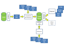
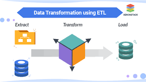
Raw data often needs to be transformed. There are many reasons why data needs to be transformed. For instance, numbers might be represented as strings in a raw data set and need to be transformed into integers or doubles to be included into a feature vector. Another reason might be the wrong unit. For instance, Fahrenheit needs to be converted into Celsius, or inch needs to be converted into metric.

Sometimes the data structure has to be transformed. Data in JSON (JavaScript Object Notation) format might have to be transformed into XML (Extensible Markup Language) format. In this case, data mapping has to be transformed since the metadata might be different in the JSON and XML file. For instance, in the source JSON file names might be denoted by “first name”, “last name” whereas in the XML it is called “given name” and “family name”. Data transformation is almost always needed in one or another form, especially if the data has more than one source.

机器学习代写

统计代写|机器学习作业代写Machine Learning代考|Feature extraction

特征提取，也称为特征选择或特征工程，是寻找隐藏知识或业务内部的最重要任务之一。在机器学习中，很少将收集的整个初始数据集用作学习算法的输入。相反，初始数据集被缩减为预期对后续机器学习任务有用且相关的数据子集。特征提取是从初始数据集中选择值的过程。特征是输入数据的独特属性，是具有代表性的描述性属性。在文献中，特征选择和特征提取之间经常存在区别[43]。特征选择意味着将特征集减少为更小的特征集或更小的特征集，因为并非所有功能都对特定任务有用。特征提取意味着将原始特征集转换为可以更好或更快地执行数据挖掘任务的新特征集。在这里，我们可以互换地处理特征提取和特征选择。如前所述，特征选择和一般数据预处理是高度特定于领域的，而机器学习算法则不是。特征选择也独立于所使用的机器学习算法。
特征不需要是直接可观察的。例如，可以使用降维技术将大量可直接观察到的特征减少为较小的一组间接可观察到的特征，也称为潜在变量或隐藏变量。特征提取-

化可以看作是降维的一种形式。通常对特征进行加权，因此并非每个特征对结果的贡献都相同。通常，权重以单独的向量呈现给学习者。
一个样本特征提取任务是词频计数。例如，对消费品的评论会更频繁地包含某些词，无论它们是正面的还是负面的。对新车的正面评价通常包含“好”、“很棒”、“优秀”等词，而不是负面评价。这里，特征提取是指定义要计数的单词并计算评论中使用正面或负面单词的次数。生成的特征向量是带有频率的单词列表。特征向量是数值特征的 n 维向量，因此实际单词不是特征向量本身的一部分。特征向量可以包含单词的哈希，如图3.1，或者这个词是通过它的索引来识别的，即向量中的位置。

统计代写|机器学习作业代写Machine Learning代考|Sampling

数据采样是选择数据子集的过程，因为分析整个数据集通常过于昂贵。抽样将实例的数量减少到要处理的子集，而不是整个数据集。可以随机选择样本，因此每个实例都有相同的被选择概率。选择过程应保证样本能够代表支配数据的分布，从而确保在样本上获得的结果与在整个数据集上获得的结果接近 [43]。

可以采用不同的方式对数据进行采样。当使用随机抽样时，每个实例都有相同的概率被选中。使用随机抽样，可以多次选择一个实例。如果从数据集中删除随机选择的实例，我们最终在样本中没有重复。

另一种抽样方法使用分层。分层用于避免样本中类标签的过度表示，并为样本提供标签的均匀分布。例如，一个样本可能包含过多的男性或女性实例。分层首先在抽样之前将数据划分为同质子组。子组应该是互斥的。它不是使用整个种群，而是分为子种群（层），一个包含女性实例的 bin 和一个包含男性实例的 bin。然后，从每个 bin 中随机选择偶数个样本。我们最终得到一个分层随机样本，其中女性和男性实例分布均匀。在将数据集划分为训练和测试子集时，也经常使用分层。两个数据集都应该具有均匀分布的特征，

统计代写|机器学习作业代写Machine Learning代考| Data transformation

原始数据通常需要转换。需要转换数据的原因有很多。例如，数字可能在原始数据集中表示为字符串，需要转换为整数或双精度才能包含到特征向量中。另一个原因可能是错误的单位。例如，华氏需要转换成摄氏度，或者英寸需要转换成公制。

有时必须转换数据结构。JSON（JavaScript 对象表示法）格式的数据可能必须转换为 XML（可扩展标记语言）格式。在这种情况下，必须转换数据映射，因为 JSON 和 XML 文件中的元数据可能不同。例如，在源 JSON 文件中，文件名可能用“名字”、“姓氏”表示，而在 XML 中则称为“给定名称”和“姓氏”。几乎总是需要以一种或另一种形式进行数据转换，尤其是在数据具有多个来源的情况下。

统计代写|机器学习作业代写Machine Learning代考请认准statistics-lab™

统计代写请认准statistics-lab™. statistics-lab™为您的留学生涯保驾护航。统计代写|python代写代考

随机过程代考

在概率论概念中，随机过程是随机变量的集合。若一随机系统的样本点是随机函数，则称此函数为样本函数，这一随机系统全部样本函数的集合是一个随机过程。实际应用中，样本函数的一般定义在时间域或者空间域。 随机过程的实例如股票和汇率的波动、语音信号、视频信号、体温的变化，随机运动如布朗运动、随机徘徊等等。

贝叶斯方法代考

贝叶斯统计概念及数据分析表示使用概率陈述回答有关未知参数的研究问题以及统计范式。后验分布包括关于参数的先验分布，和基于观测数据提供关于参数的信息似然模型。根据选择的先验分布和似然模型，后验分布可以解析或近似，例如，马尔科夫链蒙特卡罗 (MCMC) 方法之一。贝叶斯统计概念及数据分析使用后验分布来形成模型参数的各种摘要，包括点估计，如后验平均值、中位数、百分位数和称为可信区间的区间估计。此外，所有关于模型参数的统计检验都可以表示为基于估计后验分布的概率报表。

广义线性模型代考

广义线性模型（GLM）归属统计学领域，是一种应用灵活的线性回归模型。该模型允许因变量的偏差分布有除了正态分布之外的其它分布。

statistics-lab作为专业的留学生服务机构，多年来已为美国、英国、加拿大、澳洲等留学热门地的学生提供专业的学术服务，包括但不限于Essay代写，Assignment代写，Dissertation代写，Report代写，小组作业代写，Proposal代写，Paper代写，Presentation代写，计算机作业代写，论文修改和润色，网课代做，exam代考等等。写作范围涵盖高中，本科，研究生等海外留学全阶段，辐射金融，经济学，会计学，审计学，管理学等全球99%专业科目。写作团队既有专业英语母语作者，也有海外名校硕博留学生，每位写作老师都拥有过硬的语言能力，专业的学科背景和学术写作经验。我们承诺100%原创，100%专业，100%准时，100%满意。

机器学习代写

随着AI的大潮到来，Machine Learning逐渐成为一个新的学习热点。同时与传统CS相比，Machine Learning在其他领域也有着广泛的应用，因此这门学科成为不仅折磨CS专业同学的“小恶魔”，也是折磨生物、化学、统计等其他学科留学生的“大魔王”。学习Machine learning的一大绊脚石在于使用语言众多，跨学科范围广，所以学习起来尤其困难。但是不管你在学习Machine Learning时遇到任何难题，StudyGate专业导师团队都能为你轻松解决。

多元统计分析代考

基础数据: $N$ 个样本， $P$ 个变量数的单样本，组成的横列的数据表
变量定性: 分类和顺序；变量定量：数值
数学公式的角度分为: 因变量与自变量

时间序列分析代写

随机过程，是依赖于参数的一组随机变量的全体，参数通常是时间。随机变量是随机现象的数量表现，其时间序列是一组按照时间发生先后顺序进行排列的数据点序列。通常一组时间序列的时间间隔为一恒定值（如1秒，5分钟，12小时，7天，1年），因此时间序列可以作为离散时间数据进行分析处理。研究时间序列数据的意义在于现实中，往往需要研究某个事物其随时间发展变化的规律。这就需要通过研究该事物过去发展的历史记录，以得到其自身发展的规律。

回归分析代写

多元回归分析渐进（Multiple Regression Analysis Asymptotics）属于计量经济学领域，主要是一种数学上的统计分析方法，可以分析复杂情况下各影响因素的数学关系，在自然科学、社会和经济学等多个领域内应用广泛。

MATLAB代写

MATLAB 是一种用于技术计算的高性能语言。它将计算、可视化和编程集成在一个易于使用的环境中，其中问题和解决方案以熟悉的数学符号表示。典型用途包括：数学和计算算法开发建模、仿真和原型制作数据分析、探索和可视化科学和工程图形应用程序开发，包括图形用户界面构建MATLAB 是一个交互式系统，其基本数据元素是一个不需要维度的数组。这使您可以解决许多技术计算问题，尤其是那些具有矩阵和向量公式的问题，而只需用 C 或 Fortran 等标量非交互式语言编写程序所需的时间的一小部分。MATLAB 名称代表矩阵实验室。MATLAB 最初的编写目的是提供对由 LINPACK 和 EISPACK 项目开发的矩阵软件的轻松访问，这两个项目共同代表了矩阵计算软件的最新技术。MATLAB 经过多年的发展，得到了许多用户的投入。在大学环境中，它是数学、工程和科学入门和高级课程的标准教学工具。在工业领域，MATLAB 是高效研究、开发和分析的首选工具。MATLAB 具有一系列称为工具箱的特定于应用程序的解决方案。对于大多数 MATLAB 用户来说非常重要，工具箱允许您学习和应用专业技术。工具箱是 MATLAB 函数（M 文件）的综合集合，可扩展 MATLAB 环境以解决特定类别的问题。可用工具箱的领域包括信号处理、控制系统、神经网络、模糊逻辑、小波、仿真等。

R语言代写	问卷设计与分析代写
PYTHON代写	回归分析与线性模型代写
MATLAB代写	方差分析与试验设计代写
STATA代写	机器学习/统计学习代写
SPSS代写	计量经济学代写
EVIEWS代写	时间序列分析代写
EXCEL代写	深度学习代写
SQL代写	各种数据建模与可视化代写

统计代写|机器学习作业代写Machine Learning代考| Generative and discriminative models

Posted on 2022年4月14日2022年4月14日 by statistics-lab

如果你也在怎样代写机器学习Machine Learning这个学科遇到相关的难题，请随时右上角联系我们的24/7代写客服。

机器学习是人工智能（AI）和计算机科学的一个分支，主要是利用数据和算法来模仿人类的学习方式，逐步提高其准确性。

我们提供的机器学习Machine Learning及其相关学科的代写，服务范围广, 其中包括但不限于:

Statistical Inference 统计推断
Statistical Computing 统计计算
Advanced Probability Theory 高等楖率论
Advanced Mathematical Statistics 高等数理统计学
(Generalized) Linear Models 广义线性模型
Statistical Machine Learning 统计机器学习
Longitudinal Data Analysis 纵向数据分析
Foundations of Data Science 数据科学基础

统计代写|机器学习作业代写Machine Learning代考|Generative and discriminative models

Predictive algorithms are often categorized into generative and discriminative models. This distinction presumes a probabilistic perspective on machine learning algorithms. Generally speaking, a generative model learns the joint probability distribution $p(x, y)$, whereas a discriminative model learns the conditional probability distribution $p(y \mid x)$, in other words, the probability of $y$ given $x$. A generative algorithm models how the data was generated in order to categorize a signal. It is called generative since sampling can generate synthetic data points. Generative models ask the question: Based on my generation assumptions, which category is most likely to generate this signal? Generative models include naïve Bayes, Bayesian networks, Hidden Markov models (HMM) and Markov random fields (MRF).

A discriminative algorithm does not care about how the data was generated, it simply categorizes a given signal. It directly estimates posterior probabilities, they do not attempt to model the underlying probability distributions. Logistic regression, support vector machines (SVM), traditional neural networks and nearest neighbor models fall into this category. Discriminative models tend to perform better since they solve the problem directly, whereas generative models require an intermediate step. However, generative models tend to converge a lot faster.

统计代写|机器学习作业代写Machine Learning代考|Evaluation of learner

In order to evaluate the quality of a trained model, we need to evaluate how well the predictions match the observed data. In other words, we need to measure the quality of the fit. The quality is measured using a loss function or objective function. The goal of all loss functions is to measure how well an algorithm is doing against a given data set.

The loss function quantifies the extend to which the model fits the data [14], in other words, it measures the goodness of fit. During training, the machine learning algorithm tries to minimize the loss function, a process called loss minimization. We are minimizing the training loss, or training error, which is the average loss over all the training samples. A loss function calculates the price, the loss, paid for inaccuracies in a classification problem. It is, thus, also called the cost function.

There are many different loss functions. We have already seen the mean absolute error in equation 2.8. Another popular loss function is the mean squared error (MSE) since it is easy to understand and implement. The mean squared error simply takes the difference between the predictions and the ground truth, squares it, and averages it out across the whole data set. The mean squared error is always positive and the closer to zero the better. The mean squared error is computed as shown in equation $2.9$.
$$
M S E=\frac{1}{n} \sum_{i=1}^{n}\left(y_{i}-f\left(x_{i}\right)\right)^{2}
$$

where
$$
\begin{array}{ll}
y & =\text { Vector of n predictions } \
n & =\text { Number of predictions } \
f\left(x_{i}\right) & =\text { Prediction for the } i \text { th observation }
\end{array}
$$

统计代写|机器学习作业代写Machine Learning代考| Stochastic gradient descent

During training we try to minimize a loss function. So we need to make sure we learn into the right “direction” and not getting worse. For a simple loss function, we could use calculus to find the optimal parameters that minimize the loss function. However, for a more complex loss function, calculus might not be feasible anymore. One approach is to iteratively optimize the objective function by using the gradient of the function. This iterative optimization process is called gradient descent where the gradient tells us which direction to move to decrease the loss function. Figure $2.9$ shows gradient descent with a hypothetical objective function $w^{2}$ and the derivative $2 w$ that gives us the slope. If the derivative is positive, it slopes downwards to the left as shown in Figure $2.9$, if it is negative, it slopes to the right. The value of the derivative is multiplied by the constant step size $\eta$, called the learning rate, and subtracted from the current value. Once the change of the parameter value becomes too small, in Figure $2.9$ when it approaches zero, the process stops. The hyperparameter $\eta$ is the step size, which defines how fast we move to the minimum.

The problem with gradient descent is that it is slow since every iteration has to go through all the training instances, the batch, which is expensive, especially if the training set is large. The training loss is the sum over all the training data, which means, the algorithm has to go through all training instances to move one step down.

机器学习代写

统计代写|机器学习作业代写Machine Learning代考|Generative and discriminative models

预测算法通常分为生成模型和判别模型。这种区别假定了机器学习算法的概率观点。一般来说，生成模型学习联合概率分布p(X,是)，而判别模型学习条件概率分布p(是∣X)，换句话说，概率是给定X. 生成算法对如何生成数据进行建模，以便对信号进行分类。它被称为生成，因为采样可以生成合成数据点。生成模型提出了一个问题：根据我的生成假设，哪个类别最有可能生成这个信号？生成模型包括朴素贝叶斯、贝叶斯网络、隐马尔可夫模型 (HMM) 和马尔可夫随机场 (MRF)。

判别算法不关心数据是如何生成的，它只是对给定的信号进行分类。它直接估计后验概率，它们不尝试对潜在的概率分布进行建模。逻辑回归、支持向量机 (SVM)、传统神经网络和最近邻模型都属于这一类。判别模型往往表现更好，因为它们直接解决问题，而生成模型需要一个中间步骤。然而，生成模型往往收敛得更快。

统计代写|机器学习作业代写Machine Learning代考|Evaluation of learner

为了评估训练模型的质量，我们需要评估预测与观察数据的匹配程度。换句话说，我们需要衡量拟合的质量。使用损失函数或目标函数来衡量质量。所有损失函数的目标是衡量算法在给定数据集上的表现。

损失函数量化了模型拟合数据的范围[14]，换句话说，它衡量了拟合优度。在训练过程中，机器学习算法试图最小化损失函数，这个过程称为损失最小化。我们正在最小化训练损失或训练误差，这是所有训练样本的平均损失。损失函数计算为分类问题中的不准确所付出的代价，即损失。因此，它也称为成本函数。

有许多不同的损失函数。我们已经在方程 2.8 中看到了平均绝对误差。另一个流行的损失函数是均方误差 (MSE)，因为它易于理解和实现。均方误差只是取预测值和基本事实之间的差异，对其进行平方，然后在整个数据集中取平均值。均方误差始终为正，越接近零越好。均方误差的计算如等式所示2.9.
米小号和=1n∑一世=1n(是一世−F(X一世))2

在哪里
是= n 个预测的向量 n= 预测数 F(X一世)= 预测为一世观察

统计代写|机器学习作业代写Machine Learning代考| Stochastic gradient descent

在训练期间，我们尝试最小化损失函数。所以我们需要确保我们学习到正确的“方向”而不是变得更糟。对于一个简单的损失函数，我们可以使用微积分来找到最小化损失函数的最佳参数。但是，对于更复杂的损失函数，微积分可能不再可行。一种方法是通过使用函数的梯度来迭代优化目标函数。这种迭代优化过程称为梯度下降，其中梯度告诉我们向哪个方向移动以减少损失函数。数字2.9显示具有假设目标函数的梯度下降在2和导数2在这给了我们斜率。如果导数为正，则向左向下倾斜，如图所示2.9，如果为负，则向右倾斜。导数的值乘以恒定步长这，称为学习率，并从当前值中减去。一旦参数值的变化变得太小，如图2.9当它接近零时，该过程停止。超参数这是步长，它定义了我们移动到最小值的速度。

梯度下降的问题在于它很慢，因为每次迭代都必须经过所有训练实例，即批次，这很昂贵，尤其是在训练集很大的情况下。训练损失是所有训练数据的总和，这意味着算法必须遍历所有训练实例才能向下移动一步。

统计代写请认准statistics-lab™. statistics-lab™为您的留学生涯保驾护航。统计代写|python代写代考

随机过程代考

贝叶斯方法代考

广义线性模型代考

广义线性模型（GLM）归属统计学领域，是一种应用灵活的线性回归模型。该模型允许因变量的偏差分布有除了正态分布之外的其它分布。

机器学习代写

多元统计分析代考

基础数据: $N$ 个样本， $P$ 个变量数的单样本，组成的横列的数据表
变量定性: 分类和顺序；变量定量：数值
数学公式的角度分为: 因变量与自变量

时间序列分析代写

回归分析代写

MATLAB代写

R语言代写	问卷设计与分析代写
PYTHON代写	回归分析与线性模型代写
MATLAB代写	方差分析与试验设计代写
STATA代写	机器学习/统计学习代写
SPSS代写	计量经济学代写
EVIEWS代写	时间序列分析代写
EXCEL代写	深度学习代写
SQL代写	各种数据建模与可视化代写

统计代写|机器学习作业代写Machine Learning代考| k-means clustering

Posted on 2022年4月14日2022年4月14日 by statistics-lab

如果你也在怎样代写机器学习Machine Learning这个学科遇到相关的难题，请随时右上角联系我们的24/7代写客服。

机器学习是人工智能（AI）和计算机科学的一个分支，主要是利用数据和算法来模仿人类的学习方式，逐步提高其准确性。

我们提供的机器学习Machine Learning及其相关学科的代写，服务范围广, 其中包括但不限于:

Statistical Inference 统计推断
Statistical Computing 统计计算
Advanced Probability Theory 高等楖率论
Advanced Mathematical Statistics 高等数理统计学
(Generalized) Linear Models 广义线性模型
Statistical Machine Learning 统计机器学习
Longitudinal Data Analysis 纵向数据分析
Foundations of Data Science 数据科学基础

统计代写|机器学习作业代写Machine Learning代考|k-means clustering

k-means clustering is one of the most popular cluster and machine learning algorithm. k-means clustering falls into the category of centroid-based algorithms. A centroid is the geometric center of a geometric plane figure. The centroid is also called barycenter. In centroidbased clustering, $n$ observations are grouped into $k$ clusters in such a way that each observation belongs to the cluster with the nearest centroid. Here, the criterion for clustering is distance. The centroid itself does not need to be an observation point. Figure $2.7$ shows k-means clustering with 3 clusters.

In k-means clustering, the number of clusters $k$ needs to be defined beforehand, which is sometimes a problem since the number of clusters might not be known beforehand. For instance, in biology, if we want to classify plants given their features, we might not know how many different types of plants there are in a given data set. Other clustering methods, such as hierarchical clustering, do not need an assumption on the number of clusters. Also, there is no absolute criterion; it has to be defined by the user in such a way that the result of the clustering will suite the aim of the analytics task at hand. Cluster analysis is often just the starting point for other purposes, for instance a pre-processing step for other algorithms.Humans and animals learn mostly from experience, not from labeled data. Humans discover the world by observing it, not by being told the label of every object. So, human learning is largely unsupervised. That is why some authors argue that unsupervised learning will become fare more important than supervised learning in the future [18].

统计代写|机器学习作业代写Machine Learning代考|Semi-supervised learning

Semi-supervised learning uses a combination of labeled and unlabeled data. It is typically used when a small amount of labeled data and a large amount of unlabeled data is present. Since semi-supervised learning still requires labeled data, it can be considered a subset of supervised learning. However, other forms of partial supervision other than classification are possible.

Data is often labeled by a data scientist, which is a laborious task and bares the risk of introducing a human bias. Bias stems from human prejudice that, in the case of labeling data, might result in the underor overrepresentation of some features in the data set. Machine learning heavily depends on the quality of the data. If the data set is biased, the result of the machine learning task will be biased. However, human bias cannot only negatively influence machine learning through data

but also through algorithms and interaction. Human bias does not need to be conscious. It can originate from ignorance, for instance, an underrepresentation of minorities in a sample population or from a lack of data that includes minorities. Generally speaking, training data should equally represent all our world.

There are many different semi-supervised training methods. Probably the earliest idea about using unlabeled data in classification is self-learning, which is also known as self-training, self-labeling, or decision-directed learning [4]. The basic idea of self-learning is to use the labeled data set to train a learning algorithm, then use the trained learner iteratively to label chunks of the unlabeled data until all data is labeled using pseudo labels. Then the trained learner is retrained using its own predictions. Self-learning bears the risk that the pseudolabeled data will have no effect on the learner or that self-labeling happens without knowing on which assumptions the self-learning is based on. The central question for using semi-supervised learning is, under which conditions does taking into consideration unlabeled data contribute to the prediction accuracy? In the worst case, the unlabeled data will deteriorate the prediction accuracy.

统计代写|机器学习作业代写Machine Learning代考| Function approximation

Function approximation (FA) is sometimes used interchangeably with regression. Regression is a way to approximate a given data set. Function approximation can be considered a more general concept since there are many different methods to approximate data or functions. The goal of function approximation is to find a function $f$ that maps an input to an output vector. The function is selected among a defined class, e.g., quadratic functions or polynomials. For instance, equation $4.14$ is a first degree polynomial equation. Contrary to function fitting, where a curve is fitted to a set of data points, function approximation aims to find a function $f$ that approximates a target function. Given one set of samples $(x, y)$, we try to find a function $f$ :
$$
f: X \rightarrow Y
$$

where
$X=$ Input space
$Y \quad=$ Output space, number of predictions
where the input space can be multidimensional $\mathbf{X} \subseteq \mathbb{R}^{2}$, in this case $n$-dimensional. The function:
$$
f(x)=y
$$
maps $x \in X$ to $y \in Y$, where the distribution of $x$ and the function $f$ are unknown. $f$ can have some unknown properties for a space where no data points are available.

Figure $2.8$ shows an unknown function $f(x)$ and some random data points.

Function approximation is similar to regression and techniques such as interpolation, extrapolation or regression analysis can be used. Regression does essentially the same thing, create a model from a given data set. However, regression focuses more on statistical concepts, such as variance and expectation. Function approximation tries to explain the underlying data by finding a model $h(x)$ for all samples $(x, y)$, such that $h(x) \approx y$. Ideally, the model equals the underlying function $f(x)$ such

that $h(x)=f(x)$. However, there might be sub-spaces where no data points are available. To find a model, we need to measure the quality of the model. To do so, function approximation tries to minimize the prediction error. This is similar to evaluating a trained machine learning model, such as a Bayesian or a logistic regression model. An intuitive measure for the error is the mean absolute error (MAE). Given $n$ instances $(x, y)$, the model $h(x)$ can be evaluated by calculating the mean absolute error as:
$$
M A E=\frac{1}{n} \sum_{i=1}^{n}\left|y_{i}-h\left(x_{i}\right)\right|
$$

机器学习代写

统计代写|机器学习作业代写Machine Learning代考|k-means clustering

k-means 聚类是最流行的聚类和机器学习算法之一。k-means 聚类属于基于质心的算法。质心是几何平面图形的几何中心。质心也称为重心。在基于质心的聚类中，n观察被分组为到以这样一种方式进行聚类，即每个观测值都属于具有最近质心的聚类。这里，聚类的标准是距离。质心本身不需要是观察点。数字2.7显示了具有 3 个聚类的 k 均值聚类。

在 k-means 聚类中，聚类的数量到需要事先定义，这有时是个问题，因为事先可能不知道集群的数量。例如，在生物学中，如果我们想根据植物的特征对植物进行分类，我们可能不知道给定数据集中有多少种不同类型的植物。其他聚类方法，例如层次聚类，不需要对聚类数量进行假设。此外，没有绝对的标准；它必须由用户以这样一种方式定义，即聚类的结果将适合手头的分析任务的目标。聚类分析通常只是其他目的的起点，例如其他算法的预处理步骤。人类和动物主要从经验中学习，而不是从标记数据中学习。人类通过观察世界来发现世界，而不是通过被告知每个物体的标签。所以，人类学习在很大程度上是无监督的。这就是为什么一些作者认为无监督学习在未来将变得比监督学习更重要[18]。

统计代写|机器学习作业代写Machine Learning代考|Semi-supervised learning

半监督学习使用标记和未标记数据的组合。它通常在存在少量标记数据和大量未标记数据时使用。由于半监督学习仍然需要标记数据，因此可以将其视为监督学习的一个子集。然而，除分类之外的其他形式的部分监督也是可能的。

数据通常由数据科学家标记，这是一项艰巨的任务，并且存在引入人为偏见的风险。偏见源于人类的偏见，即在标记数据的情况下，可能会导致数据集中某些特征的代表性不足或过度。机器学习在很大程度上取决于数据的质量。如果数据集有偏差，机器学习任务的结果就会有偏差。然而，人为偏见不仅会通过数据对机器学习产生负面影响

而且还通过算法和交互。人类的偏见不需要有意识。它可能源于无知，例如，样本人口中少数族裔的代表性不足或缺乏包括少数族裔的数据。一般来说，训练数据应该平等地代表我们整个世界。

有许多不同的半监督训练方法。在分类中使用未标记数据的最早想法可能是自学习，也称为自训练、自标记或决策导向学习 [4]。自学习的基本思想是使用标记的数据集来训练学习算法，然后使用训练好的学习器迭代地标记未标记数据的块，直到所有数据都使用伪标签进行标记。然后使用自己的预测重新训练受过训练的学习者。自学习承担的风险是伪标记数据对学习者没有影响，或者在不知道自学习基于哪些假设的情况下发生自标记。使用半监督学习的核心问题是，在哪些条件下考虑未标记数据有助于预测准确性？在最坏的情况下，未标记的数据会降低预测精度。

统计代写|机器学习作业代写Machine Learning代考| Function approximation

函数逼近 (FA) 有时可与回归互换使用。回归是一种逼近给定数据集的方法。函数逼近可以被认为是一个更一般的概念，因为有许多不同的方法可以逼近数据或函数。函数逼近的目标是找到一个函数F将输入映射到输出向量。该函数是在定义的类中选择的，例如二次函数或多项式。例如，方程4.14是一阶多项式方程。与将曲线拟合到一组数据点的函数拟合相反，函数逼近旨在找到一个函数F逼近一个目标函数。给定一组样本(X,是)，我们试图找到一个函数F:
F:X→是

在哪里
X=输入空间
是=
输出空间，输入空间可以是多维的预测数量X⊆R2，在这种情况下n维。功能：
F(X)=是
地图X∈X到是∈是, 其中分布X和功能F是未知的。F对于没有可用数据点的空间，可能具有一些未知属性。

数字2.8显示未知功能F(X)和一些随机数据点。

函数逼近类似于回归，可以使用插值、外推或回归分析等技术。回归本质上做同样的事情，从给定的数据集创建一个模型。但是，回归更多地关注统计概念，例如方差和期望。函数逼近试图通过寻找模型来解释基础数据H(X)对于所有样品(X,是), 这样H(X)≈是. 理想情况下，模型等于底层函数F(X)这样的

那H(X)=F(X). 但是，可能存在没有数据点可用的子空间。要找到模型，我们需要衡量模型的质量。为此，函数逼近试图最小化预测误差。这类似于评估经过训练的机器学习模型，例如贝叶斯或逻辑回归模型。误差的直观度量是平均绝对误差 (MAE)。给定n实例(X,是)，该模型H(X)可以通过计算平均绝对误差来评估：
米一种和=1n∑一世=1n|是一世−H(X一世)|

统计代写请认准statistics-lab™. statistics-lab™为您的留学生涯保驾护航。统计代写|python代写代考

随机过程代考

贝叶斯方法代考

广义线性模型代考

广义线性模型（GLM）归属统计学领域，是一种应用灵活的线性回归模型。该模型允许因变量的偏差分布有除了正态分布之外的其它分布。

机器学习代写

多元统计分析代考

基础数据: $N$ 个样本， $P$ 个变量数的单样本，组成的横列的数据表
变量定性: 分类和顺序；变量定量：数值
数学公式的角度分为: 因变量与自变量

时间序列分析代写

回归分析代写

MATLAB代写

R语言代写	问卷设计与分析代写
PYTHON代写	回归分析与线性模型代写
MATLAB代写	方差分析与试验设计代写
STATA代写	机器学习/统计学习代写
SPSS代写	计量经济学代写
EVIEWS代写	时间序列分析代写
EXCEL代写	深度学习代写
SQL代写	各种数据建模与可视化代写

统计代写|机器学习作业代写Machine Learning代考|Machine Learning Basics

Posted on 2022年4月14日2022年4月14日 by statistics-lab

如果你也在怎样代写机器学习Machine Learning这个学科遇到相关的难题，请随时右上角联系我们的24/7代写客服。

机器学习是人工智能（AI）和计算机科学的一个分支，主要是利用数据和算法来模仿人类的学习方式，逐步提高其准确性。

我们提供的机器学习Machine Learning及其相关学科的代写，服务范围广, 其中包括但不限于:

Statistical Inference 统计推断
Statistical Computing 统计计算
Advanced Probability Theory 高等楖率论
Advanced Mathematical Statistics 高等数理统计学
(Generalized) Linear Models 广义线性模型
Statistical Machine Learning 统计机器学习
Longitudinal Data Analysis 纵向数据分析
Foundations of Data Science 数据科学基础

统计代写|机器学习作业代写Machine Learning代考|Machine Learning Basics

统计代写|机器学习作业代写Machine Learning代考|Supervised learning

Supervised learning needs labeled data for training. A training example is called a data point or instance and consists of an input and output pair $(x, y) . y$ is the output or ground truth for input $x$. Contrary to supervised learning, in unsupervised learning, the data only provides inputs. A multiset of training examples forms the training data set. The training data set is also called gold standard data and is as close to the ground truth as possible. The training set is used to produce a predictor function $f$, also called decision function, that maps inputs $x$ to $y=f(x)$. The goal is to produce a predictor $f$ that works with examples other than the training examples. In other words, $f$ needs to generalize beyond the training data and provide accurate predictions on new, unseen data. $f$ provides an approximation on unseen data. The input $x$ is a feature vector or covariates, the output $y$ is the response. A feature vector $\phi(x)$ is a map of feature names to feature values, i.e., strings to doubles. A feature vector $\phi(x) \in \mathbb{R}$ is a real vector $\phi(x)=\left[\phi_{1}(x), \phi_{2}(x), \ldots \phi_{n}(x)\right]$, where each component $\phi_{i}(x)$ with $i=1, \ldots n$ represents a feature. The feature vector is computed by the feature extractor $\phi$ and can be thought of as a point in a high-dimensional feature space. A feature in a feature vector can be weighted, which means, not every feature necessarily contributes equally to a prediction. A weight is a real number that is multiplied with the feature value. The weights are represented in a separate weight vector because we want one single predictor that works on any input. Given a feature vector $\phi(x)$ and a weight vector $w$, we calculate the prediction score as the inner product of the vectors $w \cdot \phi(x)$. We do

not know the weights in vector $w$ beforehand, they are learned during training.

To predict, for instance, if a news article is about politics or sports, we need to find out what properties of input $x$ might be relevant to predict if the article belongs to the category “politics” or “sports”. This process is called feature extraction. There are machine learning techniques where no function is generated. For example, decision tree induction creates a decision tree, as the name suggests, usually represented as a dendrogram and not a function. To begin with, we will start with a function and explain other techniques in later chapters.

If we try to classify the data into categories, e.g., medical images into healthy or pathologic tissue, we have a classification problem. Classification has discrete outputs such as “true” or “false” or “0” or ” 1 “. If there are just two categories, it is a binary classification problem. Often, the outputs are probabilities, e.g., a mail is spam with 80 percent probability. In other words, the dichotomy of the output is not imperative.

If there are more categories, e.g., restaurant reviews using a Likert scale, as shown in Figure 2.2, it is a multiclass classification problem.

统计代写|机器学习作业代写Machine Learning代考|Perceptron

The perceptron is a simple neural network, proposed in 1958 by Rosenblatt, which became a landmark in early machine learning history [10]. It is one of the oldest machine learning algorithms. The perceptron consists of a single neuron and is a binary classifier that can linearly separate an input $x$, a real valued vector, into a single, binary output. It is an online learning algorithm. Online learning means it processes one input at a time. The data is presented in a sequential order and updates the predictor at each step using the best predictor. The perceptron is

modeled after a neuron in the brain and is the basic element of a neural network.

There are different types of perceptrons. They can have one or more input and output links. The input links correspond to the dendrites of a real neuron, the output links to the synapses. Also, there are different types of activation functions. The perceptron shown in Figure $2.3$ consists of three weighted input links, a sum function, a step activation function and one output link.
A perceptron performs three processing steps:

Each input signal $x$ is multiplied by a weight $w: w_{i} x_{i}$
All signals are summed up
The summed up inputs are fed to an activation function
The output is calculated using the output function $f(x)$, as defined by equation 2.3.
$$
f(x)=\sum_{i=1} w_{i} x_{i}+b
$$
where
$$
\begin{aligned}
w &=\text { Weight } \
x &=\text { Input } \
b &=\text { Bias }
\end{aligned}
$$

统计代写|机器学习作业代写Machine Learning代考| Unsupervised learning

In supervised learning, we have input and output data. In unsupervised learning, we do not have labeled training data. In other words, we only

have input data, no output data, i.e., there is no $y$. Instead of predicting or approximating a variable, we try to group the data into different classes. For instance, we have a population of online shop users that we try to segment into different types of buyers. The types could be social shopper, lifestyle junkie and detached introvert. In this case, we have three clusters. If an observation point can only belong to one cluster, it is an exclusive cluster, if it is allowed to be part of more than one cluster, it is a non-exclusive cluster, in other words, the clusters can be overlapping.

Let $N$ be a set of unlabeled instances $D=x_{1}, x_{2}, \ldots, x_{N}$ in a $d$ dimensional feature space, in clustering $D$ is partitioned into a number of disjoint subsets $D_{j} \mathrm{~s}$ :
$$
D=\cup_{j=1}^{k} D_{j}
$$
where
$$
\begin{aligned}
&D_{i} \cap D_{j}=\emptyset \
&i \neq j
\end{aligned}
$$
The points in each subset $D_{j}$ are similar to each other according to a given criterion $\varnothing$. Similarity is usually expressed by some distance measure, such as the Euclidean distance or Manhattan distance.

Cluster analysis can be used for understanding the underlying structure of a dataset by grouping it into classes based on similarities. Grouping similar objects into conceptually meaningful classes has many reallife applications. For instance, biologists spent a considerable amount of time on grouping plants and animals into classes, such as rodents, canines, felines, ruminants, marsupials, etc. Clustering is also used for information retrieval, for instance, by grouping Web search results into categories, such as news, social media, blogs, forums, marketing, etc. Each category can then be divided into subcategories. For example, news is divided into politics, economics, sports, etc. This process is called hierarchical clustering. Humans, even young children, are skilled at grouping objects into their corresponding classes. This capability is important to humans for understanding and describing the world around us. This is crucial for our survival. We need to know which groups of animals are harmful or which traffic situations are potentially dangerous.

机器学习代写

统计代写|机器学习作业代写Machine Learning代考|Supervised learning

监督学习需要标记数据进行训练。训练示例称为数据点或实例，由输入和输出对组成(X,是).是是输入的输出或基本事实X. 与监督学习相反，在无监督学习中，数据仅提供输入。多组训练示例形成训练数据集。训练数据集也称为黄金标准数据，并且尽可能接近真实数据。训练集用于产生预测函数F，也称为决策函数，映射输入X到是=F(X). 目标是产生一个预测器F它适用于训练示例以外的示例。换句话说，F需要在训练数据之外进行泛化，并对新的、看不见的数据提供准确的预测。F提供对未见数据的近似值。输入X是特征向量或协变量，输出是是响应。一个特征向量φ(X)是特征名称到特征值的映射，即字符串到双精度。一个特征向量φ(X)∈R是一个实向量φ(X)=[φ1(X),φ2(X),…φn(X)], 其中每个分量φ一世(X)和一世=1,…n代表一个特征。特征向量由特征提取器计算φ并且可以被认为是高维特征空间中的一个点。可以对特征向量中的特征进行加权，这意味着并非每个特征都必须对预测做出同等贡献。权重是与特征值相乘的实数。权重在一个单独的权重向量中表示，因为我们想要一个适用于任何输入的单个预测器。给定一个特征向量φ(X)和一个权重向量在，我们将预测分数计算为向量的内积在⋅φ(X). 我们的确是

不知道向量中的权重在事先，它们是在培训期间学习的。

例如，要预测一篇新闻文章是否是关于政治或体育的，我们需要找出输入的哪些属性X可能与预测文章是否属于“政治”或“体育”类别相关。这个过程称为特征提取。有些机器学习技术不会生成任何函数。例如，决策树归纳创建决策树，顾名思义，通常表示为树状图而不是函数。首先，我们将从一个函数开始，并在后面的章节中解释其他技术。

如果我们试图将数据分类，例如将医学图像分类为健康或病理组织，我们就会遇到分类问题。分类具有离散输出，例如“真”或“假”或“0”或“1”。如果只有两个类别，这是一个二元分类问题。通常，输出是概率，例如，邮件是垃圾邮件，概率为 80%。换句话说，输出的二分法不是必须的。

如果有更多的类别，例如使用李克特量表的餐厅评论，如图 2.2 所示，这是一个多类分类问题。

统计代写|机器学习作业代写Machine Learning代考|Perceptron

感知器是一个简单的神经网络，由 Rosenblatt 于 1958 年提出，成为早期机器学习历史上的里程碑[10]。它是最古老的机器学习算法之一。感知器由单个神经元组成，是一个可以线性分离输入的二元分类器X，一个实值向量，转换为单个二进制输出。它是一种在线学习算法。在线学习意味着它一次处理一个输入。数据按顺序呈现，并在每一步使用最佳预测器更新预测器。感知器是

以大脑中的神经元为模型，是神经网络的基本元素。

有不同类型的感知器。它们可以有一个或多个输入和输出链接。输入链接对应于真实神经元的树突，输出链接对应于突触。此外，还有不同类型的激活函数。如图所示的感知器2.3由三个加权输入链接、一个求和函数、一个步进激活函数和一个输出链接组成。
感知器执行三个处理步骤：

每个输入信号X乘以权重在:在一世X一世
汇总所有信号
总和的输入被馈送到激活函数
使用输出函数计算输出F(X)，如公式 2.3 所定义。
F(X)=∑一世=1在一世X一世+b
在哪里
在= 重量 X= 输入 b= 偏见

统计代写|机器学习作业代写Machine Learning代考| Unsupervised learning

在监督学习中，我们有输入和输出数据。在无监督学习中，我们没有标记的训练数据。换句话说，我们只

有输入数据，没有输出数据，即没有是. 我们不是预测或近似变量，而是尝试将数据分组到不同的类别中。例如，我们有一群在线商店用户，我们试图将这些用户细分为不同类型的买家。这些类型可能是社交购物者、生活方式迷和超然内向的人。在这种情况下，我们有三个集群。如果一个观察点只能属于一个簇，则为排他簇，如果允许属于多个簇，则为非排他簇，即簇可以重叠。

让ñ是一组未标记的实例D=X1,X2,…,Xñ在一个d维度特征空间，在聚类中D被分割成许多不相交的子集Dj s:
D=∪j=1到Dj
在哪里
D一世∩Dj=∅ 一世≠j
每个子集中的点Dj根据给定的标准彼此相似∅. 相似度通常用一些距离度量来表示，例如欧几里得距离或曼哈顿距离。

聚类分析可用于通过基于相似性将数据集分组为类来理解数据集的底层结构。将相似的对象分组到概念上有意义的类中具有许多实际应用。例如，生物学家花费大量时间将植物和动物分组，如啮齿动物、犬科动物、猫科动物、反刍动物、有袋动物等。聚类也用于信息检索，例如，通过将网络搜索结果分组，例如新闻、社交媒体、博客、论坛、营销等。然后每个类别都可以分为子类别。例如，新闻分为政治、经济、体育等，这个过程称为层次聚类。人类，甚至是年幼的孩子，都擅长将对象分组到相应的类别中。这种能力对于人类理解和描述我们周围的世界很重要。这对我们的生存至关重要。我们需要知道哪些动物群是有害的，或者哪些交通状况有潜在危险。

统计代写请认准statistics-lab™. statistics-lab™为您的留学生涯保驾护航。统计代写|python代写代考

随机过程代考

贝叶斯方法代考

广义线性模型代考

广义线性模型（GLM）归属统计学领域，是一种应用灵活的线性回归模型。该模型允许因变量的偏差分布有除了正态分布之外的其它分布。

机器学习代写

多元统计分析代考

基础数据: $N$ 个样本， $P$ 个变量数的单样本，组成的横列的数据表
变量定性: 分类和顺序；变量定量：数值
数学公式的角度分为: 因变量与自变量

时间序列分析代写

回归分析代写

MATLAB代写

R语言代写	问卷设计与分析代写
PYTHON代写	回归分析与线性模型代写
MATLAB代写	方差分析与试验设计代写
STATA代写	机器学习/统计学习代写
SPSS代写	计量经济学代写
EVIEWS代写	时间序列分析代写
EXCEL代写	深度学习代写
SQL代写	各种数据建模与可视化代写

统计代写|机器学习作业代写Machine Learning代考|Unsupervised learning

Posted on 2022年4月14日2022年4月14日 by statistics-lab

如果你也在怎样代写机器学习Machine Learning这个学科遇到相关的难题，请随时右上角联系我们的24/7代写客服。

机器学习是人工智能（AI）和计算机科学的一个分支，主要是利用数据和算法来模仿人类的学习方式，逐步提高其准确性。

我们提供的机器学习Machine Learning及其相关学科的代写，服务范围广, 其中包括但不限于:

Statistical Inference 统计推断
Statistical Computing 统计计算
Advanced Probability Theory 高等楖率论
Advanced Mathematical Statistics 高等数理统计学
(Generalized) Linear Models 广义线性模型
Statistical Machine Learning 统计机器学习
Longitudinal Data Analysis 纵向数据分析
Foundations of Data Science 数据科学基础

统计代写|机器学习作业代写Machine Learning代考|Unsupervised learning

Unsupervised learning techniques are used when no labeled data is present. In other words, there is no $y$. One of the most popular unsupervised approaches is clustering. The goal of clustering is to understand the data by finding the underlying structure of data. Clustering groups data based on some similarity measure. For instance, a company groups it’s online users into customer groups with similar purchasing behavior and demographics in order to better target them with a marketing campaign. In this example the similarities are the purchasing habits and the age group. Since there is no labeled data, evaluating a cluster is not an obvious task to do. There is no ground truth that the result of a clustering task can be compared with.

Clustering can also be used to represent data in a more compressed format (dimensionality reduction), for data summarization, while keeping it’s structure and usefulness. Clustering can also be used as a preliminary step for supervised machine learning algorithms, for instance,

to reduce dimensionality to improve performance of the supervised learner.

Typical clustering algorithms include k-means clustering, hierarchical clustering or principal component analysis (PCA). In k-means clustering, the algorithm groups data points into $k$ groups where $k$ is the center of a group and is called centroid. The centroid is also called geometric center or barycenter and represents the mean position of all the data points of a cluster group. In k-means clustering, the data points are grouped around the centroids. The points closest to the centroid $k$ are added to the cluster. For instance, a warehouse inventory is grouped by sales activity or sensor data in an Internet of Things (IoT) application is grouped into normal and deviant sensor data for anomaly detection.
In k-means clustering, the number of $k$ has to be defined beforehand. Selecting the number of clusters is not always an obvious task to do. For instance, grouping images of animals into their biological families such as felines, canines, etc., requires prior knowledge about how many families there are going to be in the images to be clustered. kmeans is easy and converges quickly, which often makes it a good starting point for a machine learning project.

Hierarchical clustering or hierarchical cluster analysis (HCA), groups data by creating a tree or dendrogram. There are two approaches, a bottom up or agglomerative approach, where each data point starts in it’s own cluster, and the top down or divisive approach, where all observations are put into one cluster and splits are performed in order to create a hierarchy that is usually presented as a dendrogram.

Human and animal learning is largely unsupervised. Humans learn from observing the world, not by being told the label of every object, making unsupervised learning more biologically plausible.

统计代写|机器学习作业代写Machine Learning代考|Semi-supervised learning

Semi-supervised learning is typically used when a small amount of labelled data and a large amount of unlabelled data is present. Labeling

data is often a manual and laborious task for a data scientist. This bares the danger of introducing a human bias on the model. Using semisupervised methods can often increase the accuracy of the model and, at the same time, reduce the time and cost for producing a model since not all data needs to be labeled. For instance, manually labelling data for gene sequencing is an insurmountable task for a data scientist due to the large volumes of data; there are approximately six billion base pairs in a human, diploid genome. Semi-supervised methods can alleviate this problem by only labelling a small amount of data. In other words, the features are learned from a small amount of labelled data. First, we train a model with the small amount of labeled data. Then we label the unlabeled data set with the trained model that gave the best results. This yields a large volume of pseudo-labeled data. We now combine the labeled and pseudo-labeled data sets in order to train a model. This way, we should be able to better capture the underlying data distribution and the model generalizes better. As usual, there are other semi-supervised techniques. Semi-supervised methods give access to large amounts of data for training while minimizing the time spent for labeling training data. Ideally, semi-supervised methods can even reveal new labels.

Semi-supervised learning can be associated to human concept learning. Parents tell children the name of an object or animal when they see it the first time, they label it. The small amount of parental labelling suffices for children to be able to label new objects when they see them.

统计代写|机器学习作业代写Machine Learning代考|Machine learning and statistics

Machine learning uses a lot of statistics. That is why you will often find statistical terms and machine learning terms used interchangeably in literature. For instance, the terms dependent and independent variable are statistical terms, feature and label are their machine learning equivalents. Table $1.1$ opposes some popular machine learning terms and their corresponding statistical terms.

The term statistical learning is sometimes confused with machine learning. There is a subtle difference between the two methods. Both

methods are data-based. However, machine learning uses data to improve the performance of a system. Statistical learning is based on a hypothesis. The basic assumption in statistical learning is that the data share some properties with a certain regularity. Therefore, statistical learning can use probabilistic methods and probabilistic distributions can be used to describe the statistical regularity. Machine learning is not based on assumptions. Statistical learning is math intensive and usually uses smaller data sets with fewer features, whereas machine learning can use billions of instances and features. Statistical learning requires a good understanding of the data, whereas machine learning can identify patterns iteratively with much less human effort. Therefore, machine learning is often preferred over statistical learning. However, since statistical learning requires us to familiarize ourselves with the data, it helps us gain more confidence in our model.

Machine learning is sometimes criticised as just being glorified statistics. Whereas it is true that machine learning uses a lot of statistics, machine learning also uses other concepts, such as data mining or neurocomputing, and is, as such, a subarea of computer science. Statistics is a subarea of mathematics. Both, machine learning and statistical learning are methods that learn from data. However, machine learning is an algorithm that learns from data without the need to be programmed by a developer. Statistical learning is a mathematical formalization of relationships between variables in the form of equations.

机器学习代写

统计代写|机器学习作业代写Machine Learning代考|Unsupervised learning

当不存在标记数据时，使用无监督学习技术。换句话说，没有是. 最流行的无监督方法之一是聚类。聚类的目标是通过找到数据的底层结构来理解数据。聚类基于某种相似性度量对数据进行分组。例如，一家公司将其在线用户分组到具有相似购买行为和人口统计数据的客户群中，以便通过营销活动更好地定位他们。在这个例子中，相似之处是购买习惯和年龄组。由于没有标记数据，因此评估集群并不是一项显而易见的任务。没有可以比较聚类任务结果的基本事实。

聚类还可用于以更压缩的格式（降维）表示数据，用于数据汇总，同时保持其结构和有用性。聚类也可以用作监督机器学习算法的初步步骤，例如，

降低维度以提高监督学习器的性能。

典型的聚类算法包括 k-means 聚类、层次聚类或主成分分析 (PCA)。在 k-means 聚类中，算法将数据点分组为到团体在哪里到是群的中心，称为质心。质心也称为几何中心或重心，表示一个聚类组中所有数据点的平均位置。在 k-means 聚类中，数据点围绕质心进行分组。离质心最近的点到被添加到集群中。例如，仓库库存按销售活动分组，或者物联网 (IoT) 应用程序中的传感器数据被分组为正常和异常传感器数据以进行异常检测。
在 k-means 聚类中，到必须事先定义。选择集群的数量并不总是一项显而易见的任务。例如，将动物的图像分组到它们的生物家族中，如猫科动物、犬科动物等，需要先验知道图像中有多少个家庭将被聚类。kmeans 简单且收敛迅速，这通常使其成为机器学习项目的良好起点。

层次聚类或层次聚类分析 (HCA) 通过创建树或树状图对数据进行分组。有两种方法，一种是自下而上或凝聚的方法，其中每个数据点都从其自己的集群开始，另一种是自上而下或分裂的方法，其中所有观察结果都放在一个集群中并执行拆分以创建一个层次结构，即通常呈现为树状图。

人类和动物的学习在很大程度上是无监督的。人类通过观察世界来学习，而不是通过被告知每个物体的标签来学习，这使得无监督学习在生物学上更加合理。

统计代写|机器学习作业代写Machine Learning代考|Semi-supervised learning

当存在少量标记数据和大量未标记数据时，通常使用半监督学习。标签

对于数据科学家来说，数据通常是一项手动且费力的任务。这暴露了在模型中引入人为偏见的危险。使用半监督方法通常可以提高模型的准确性，同时减少生成模型的时间和成本，因为并非所有数据都需要标记。例如，由于数据量很大，为基因测序手动标记数据对于数据科学家来说是一项难以逾越的任务；人类二倍体基因组中大约有 60 亿个碱基对。半监督方法可以通过仅标记少量数据来缓解这个问题。换句话说，这些特征是从少量标记数据中学习的。首先，我们用少量标记数据训练模型。然后我们用经过训练的模型来标记未标记的数据集，该模型给出了最好的结果。这会产生大量的伪标记数据。我们现在结合标记和伪标记数据集来训练模型。这样，我们应该能够更好地捕获底层数据分布，并且模型可以更好地泛化。像往常一样，还有其他半监督技术。半监督方法可以访问大量数据进行训练，同时最大限度地减少标记训练数据所花费的时间。理想情况下，半监督方法甚至可以揭示新标签。半监督方法可以访问大量数据进行训练，同时最大限度地减少标记训练数据所花费的时间。理想情况下，半监督方法甚至可以揭示新标签。半监督方法可以访问大量数据进行训练，同时最大限度地减少标记训练数据所花费的时间。理想情况下，半监督方法甚至可以揭示新标签。

半监督学习可以与人类概念学习相关联。当孩子第一次看到物体或动物时，父母会告诉他们它的名字，然后给它贴上标签。少量的父母标签就足以让孩子们在看到新物体时给它们贴上标签。

统计代写|机器学习作业代写Machine Learning代考|Machine learning and statistics

机器学习使用大量统计数据。这就是为什么您经常会发现统计术语和机器学习术语在文献中可以互换使用。例如，术语因变量和自变量是统计术语，特征和标签是它们的机器学习等价物。桌子1.1反对一些流行的机器学习术语及其对应的统计术语。

统计学习一词有时会与机器学习相混淆。这两种方法之间存在细微差别。两个都

方法是基于数据的。但是，机器学习使用数据来提高系统的性能。统计学习基于假设。统计学习的基本假设是数据具有一定的规律性。因此，统计学习可以使用概率方法，概率分布可以用来描述统计规律。机器学习不是基于假设。统计学习是数学密集型的，通常使用具有较少特征的较小数据集，而机器学习可以使用数十亿个实例和特征。统计学习需要对数据有很好的理解，而机器学习可以用更少的人力来迭代地识别模式。因此，机器学习通常比统计学习更受欢迎。然而，

机器学习有时被批评为只是美化的统计数据。虽然机器学习确实使用了大量统计数据，但机器学习还使用其他概念，例如数据挖掘或神经计算，因此是计算机科学的一个子领域。统计学是数学的一个子领域。机器学习和统计学习都是从数据中学习的方法。但是，机器学习是一种无需开发人员编程即可从数据中学习的算法。统计学习是以方程的形式对变量之间的关系进行数学形式化。

统计代写请认准statistics-lab™. statistics-lab™为您的留学生涯保驾护航。统计代写|python代写代考

随机过程代考

贝叶斯方法代考

广义线性模型代考

广义线性模型（GLM）归属统计学领域，是一种应用灵活的线性回归模型。该模型允许因变量的偏差分布有除了正态分布之外的其它分布。

机器学习代写

多元统计分析代考

基础数据: $N$ 个样本， $P$ 个变量数的单样本，组成的横列的数据表
变量定性: 分类和顺序；变量定量：数值
数学公式的角度分为: 因变量与自变量

时间序列分析代写

回归分析代写

MATLAB代写

R语言代写	问卷设计与分析代写
PYTHON代写	回归分析与线性模型代写
MATLAB代写	方差分析与试验设计代写
STATA代写	机器学习/统计学习代写
SPSS代写	计量经济学代写
EVIEWS代写	时间序列分析代写
EXCEL代写	深度学习代写
SQL代写	各种数据建模与可视化代写

统计代写|机器学习作业代写Machine Learning代考|Data pre-processing

Posted on 2022年4月14日2022年4月14日 by statistics-lab

如果你也在怎样代写机器学习Machine Learning这个学科遇到相关的难题，请随时右上角联系我们的24/7代写客服。

机器学习是人工智能（AI）和计算机科学的一个分支，主要是利用数据和算法来模仿人类的学习方式，逐步提高其准确性。

我们提供的机器学习Machine Learning及其相关学科的代写，服务范围广, 其中包括但不限于:

Statistical Inference 统计推断
Statistical Computing 统计计算
Advanced Probability Theory 高等楖率论
Advanced Mathematical Statistics 高等数理统计学
(Generalized) Linear Models 广义线性模型
Statistical Machine Learning 统计机器学习
Longitudinal Data Analysis 纵向数据分析
Foundations of Data Science 数据科学基础

统计代写|机器学习作业代写Machine Learning代考|Data pre-processing

A problem that plagues practical machine learning is poor quality of the data [40]. Real world data is often noisy and inconsistent and cannot be used as is for practical machine learning applications. Also, real world data is seldom in a format that can be directly used as input for a machine learning scheme. That is why data pre-processing is needed. Data pre-processing is usually where most of the time is spent. It is not unusual that it takes up to $70 \%$ of the effort in a data mining project.
Whereas machine learning techniques are domain independent, data pre-processing is highly domain specific. For instance, depending on whether text data is analyzed or images, different pre-processing steps apply. The pre-processing tasks also depend on the learning algorithm applied. Some algorithms can handle noise better than others. For instance, linear regression is very sensitive to outliers, which makes outlier removal a mandatory pre-processing step.

There are many different pre-processing techniques. Typical data preprocessing tasks next to outlier removal include relevance filtering, data deduplication, data transformation, entity resolution and data enrichment. For instance, going back to the spam filter example, spam mails typically contain words or phrases such as “buy online”, “online pharmacy” or hyperlinks more often than legitimate mails. The frequency of certain words or phrases gives an indication of whether the mail is spam or legitimate. Irrelevant words, characters or symbols are first removed from the mail, a process called stop word removal. There is no authoritative list of stop words and they depend on what is being mined for. Stop words are the most common words in a language, e.g., “the”, “who”,” “that”. After stop word removal, the frequencies of the remaining words are counted, to create a word list with their frequencies. The resulting list is called a bag-of-words. The bag-of-words is then used as input for a machine learning scheme. Figure $1.2$ shows an email before and after pre-processing.

统计代写|机器学习作业代写Machine Learning代考|Data analysis

Data analysis is the process of knowledge discovery. During the data analysis phase, the predictive model is created. There are many data analysis methods that do not use machine learning techniques. However, this book focuses on data analysis using machine learning, other methods are beyond the scope of this book.

Machine learning is divided into supervised, semi-supervised and unsupervised learning. Some widely-used learning methods include ensemble learning, reinforcement learning and active learning. Ensemble learning combines several supervised methods to form a stronger learner. Reinforcement learning are reward-based algorithms which learn how to attain a complex objective, the goal. Active learning is a special form of semi-supervised learning.

统计代写|机器学习作业代写Machine Learning代考|Supervised learning

Supervised learning techniques are applied when labeled data is present. The labeled data is used for training and testing. Labeling is often a manual process and can be time consuming and expensive. Every training data record is associated with the correct label. For spam filtering, labeled data will mean a data set of spam and of legitimate mails. Here, the labels are “spam” and “legitimate”. During training, the machine learning algorithm learns the relationship between the email and the associated label, “spam” or “legitimate”. The learned relationship is then used for classifying new emails that the learner has not seen before into their corresponding category.

Supervised methods can be used for classification and regression. Classification groups data into categories. Spam filtering is a classification problem since mails are classified into spam and legitimate mails. The classes are the labels. Since there are two categories, it it a binary clas-

sification problem. If there are more than two classes, it is called a multi-class or multi-label classification problem.

Regression analysis is used for estimating the relationship among variables. It tries to determine the strength of the relationship between a series of changing variables, the independent variables, usually denoted by $X$, and the dependent variable, usually denoted by $Y$. If there is one dependent variable, it is called simple linear regression, if there is more than one dependent variable, it is called multiple linear regression. In classification, you are looking for a label, in regression for a number. Predicting if it is going to rain tomorrow is a classification problem where the labels are “rainy” or “sunny”, predicting how many millimeters it is going to rain is a regression problem. The target or dependent variable $y$ is a continuous variable. Contrarily, discrete variables take on a finite number of values. Typical supervised methods are Bayesian models, artificial neural networks, support vector machines, k-nearest neighbor, regression models and decision tree induction.

机器学习代写

统计代写|机器学习作业代写Machine Learning代考|Data pre-processing

困扰实际机器学习的一个问题是数据质量差[40]。现实世界的数据通常是嘈杂且不一致的，不能按原样用于实际的机器学习应用程序。此外，现实世界的数据很少采用可以直接用作机器学习方案输入的格式。这就是为什么需要数据预处理的原因。数据预处理通常是花费大部分时间的地方。它需要多达70%数据挖掘项目的努力。
机器学习技术是独立于领域的，而数据预处理是高度特定于领域的。例如，根据是分析文本数据还是分析图像，应用不同的预处理步骤。预处理任务还取决于所应用的学习算法。一些算法可以比其他算法更好地处理噪声。例如，线性回归对异常值非常敏感，这使得去除异常值成为强制性的预处理步骤。

有许多不同的预处理技术。除异常值外，典型的数据预处理任务包括相关性过滤、重复数据删除、数据转换、实体解析和数据丰富。例如，回到垃圾邮件过滤器的例子，垃圾邮件通常比合法邮件更频繁地包含诸如“在线购买”、“在线药房”或超链接之类的词或短语。某些单词或短语的频率表明邮件是垃圾邮件还是合法邮件。首先从邮件中删除不相关的单词、字符或符号，这个过程称为停用词删除。没有权威的停用词列表，它们取决于所挖掘的内容。停用词是一种语言中最常见的词，例如“the”、“who”、“that”。去除停用词后，计算剩余单词的频率，以创建具有频率的单词列表。结果列表称为词袋。然后将词袋用作机器学习方案的输入。数字1.2显示预处理前后的电子邮件。

统计代写|机器学习作业代写Machine Learning代考|Data analysis

数据分析是知识发现的过程。在数据分析阶段，创建预测模型。有许多数据分析方法不使用机器学习技术。但是，本书侧重于使用机器学习进行数据分析，其他方法超出了本书的范围。

机器学习分为监督学习、半监督学习和无监督学习。一些广泛使用的学习方法包括集成学习、强化学习和主动学习。集成学习结合了几种监督方法来形成更强的学习器。强化学习是基于奖励的算法，它学习如何实现一个复杂的目标，即目标。主动学习是半监督学习的一种特殊形式。

统计代写|机器学习作业代写Machine Learning代考|Supervised learning

当存在标记数据时，将应用监督学习技术。标记的数据用于训练和测试。贴标签通常是一个手动过程，既耗时又昂贵。每个训练数据记录都与正确的标签相关联。对于垃圾邮件过滤，标记数据意味着垃圾邮件和合法邮件的数据集。在这里，标签是“垃圾邮件”和“合法”。在训练期间，机器学习算法会学习电子邮件与相关标签“垃圾邮件”或“合法”之间的关系。然后，学习到的关系用于将学习者以前未见过的新电子邮件分类到相应的类别中。

监督方法可用于分类和回归。分类将数据分组。垃圾邮件过滤是一个分类问题，因为邮件分为垃圾邮件和合法邮件。类是标签。由于有两个类别，它是一个二进制类-

规格化问题。如果有两个以上的类，则称为多类或多标签分类问题。

回归分析用于估计变量之间的关系。它试图确定一系列变化变量之间的关系强度，即自变量，通常表示为X和因变量，通常表示为是. 如果有一个因变量，则称为简单线性回归，如果有多个因变量，则称为多元线性回归。在分类中，您正在寻找标签，在回归中寻找数字。预测明天是否会下雨是一个分类问题，其中标签是“下雨”或“晴天”，预测下雨多少毫米是一个回归问题。目标或因变量是是一个连续变量。相反，离散变量具有有限数量的值。典型的监督方法是贝叶斯模型、人工神经网络、支持向量机、k-最近邻、回归模型和决策树归纳。

统计代写请认准statistics-lab™. statistics-lab™为您的留学生涯保驾护航。统计代写|python代写代考

随机过程代考

贝叶斯方法代考

广义线性模型代考

广义线性模型（GLM）归属统计学领域，是一种应用灵活的线性回归模型。该模型允许因变量的偏差分布有除了正态分布之外的其它分布。

机器学习代写

多元统计分析代考

基础数据: $N$ 个样本， $P$ 个变量数的单样本，组成的横列的数据表
变量定性: 分类和顺序；变量定量：数值
数学公式的角度分为: 因变量与自变量

时间序列分析代写

回归分析代写

MATLAB代写

R语言代写	问卷设计与分析代写
PYTHON代写	回归分析与线性模型代写
MATLAB代写	方差分析与试验设计代写
STATA代写	机器学习/统计学习代写
SPSS代写	计量经济学代写
EVIEWS代写	时间序列分析代写
EXCEL代写	深度学习代写
SQL代写	各种数据建模与可视化代写

统计代写|机器学习作业代写Machine Learning代考|Liquidity Augmented Expected Shortfall

Posted on 2022年4月14日2022年4月14日 by statistics-lab

如果你也在怎样代写机器学习Machine Learning这个学科遇到相关的难题，请随时右上角联系我们的24/7代写客服。

机器学习是人工智能（AI）和计算机科学的一个分支，主要是利用数据和算法来模仿人类的学习方式，逐步提高其准确性。

我们提供的机器学习Machine Learning及其相关学科的代写，服务范围广, 其中包括但不限于:

Statistical Inference 统计推断
Statistical Computing 统计计算
Advanced Probability Theory 高等楖率论
Advanced Mathematical Statistics 高等数理统计学
(Generalized) Linear Models 广义线性模型
Statistical Machine Learning 统计机器学习
Longitudinal Data Analysis 纵向数据分析
Foundations of Data Science 数据科学基础

统计代写|机器学习作业代写Machine Learning代考|Liquidity Augmented Expected Shortfall

统计代写|机器学习作业代写Machine Learning代考|Data mining

Data mining (DM) is defined as the process of discovering patterns in data [40]. There is no clear distinction in literature between data mining and machine learning. In some publications, data mining focuses on extracting data patterns and finding relationships between data [10], whereas machine learning focuses on making predictions [36]. Data mining is the process of discovering useful patterns and trends in large data sets. Predictive analytics is the process of extracting information from large data sets in order to make predictions and estimates about future outcomes [17]. Therefore the distinction is in the aim. Data mining aims to interpret data, to find patterns that can explain some phenomenon. Machine learning on the other hand, aims to make predictions by building models that can foresee some future outcome. However, clustering is a machine learning technique that aims to understand the underlying structure of the data and has similar goals to data mining. Here, we treat machine learning as a subarea of data mining where the rules are learned automatically.

Humans learn from experience, machines learn from data. Data is the starting point for all machine learning projects. Machine learning techniques learn the rules from historic data in order to create an inner representation, an abstraction, that is often difficult to interpret. Programming computers to learn from experience should eventually eliminate the need for much of this detailed programming effort [35].

统计代写|机器学习作业代写Machine Learning代考|Data mining steps

A typical data mining workflow goes through several steps. These steps include data collection, cleansing, transformation, aggregation, modeling, predictive analysis, visualization and dissemination. However, depending on the problem at hand, those steps might vary or additional steps might be necessary. Data mining requires domain specific knowledge. If a data mining project is supposed to detect fraud and money laundering in financial transactions or group news articles into categories such as “Politics”, “Business”, “Science” etc., different techniques apply. Getting familiar with the domain of the application and setting the goals of the data mining project are necessary preliminary tasks in order for the data mining project to complete successfully. Domain knowledge is also necessary to evaluate the performance of a trained learner. Figure $1.1$ summarizes the data mining steps.Data mining is a highly iterative process and typically goes through many iterations until satisfactory results are achieved. Data mining projects have to be executed with great care. The growth of data in the past years has fostered the development of new data mining applications where the internal workings often go undocumented. The blackbox approach is dangerous since the results can be difficult to explain, or lead to erroneous conclusions. For instance, cancer tissue in medical images that was undetected or a traffic situation that was misinterpreted by an autonomously driving car. The ease with which these applications can manipulate data, combined with the power of the formidable data mining algorithms embedded in the black-box software, make their misuse proportionally more hazardous [17]. Ultimately, one canfind anything in data and if a machine learning project is carried out without proficiency it can lead to expensive failures.

统计代写|机器学习作业代写Machine Learning代考|Data collection

Data collection is the process of tapping into data sources and extracting the data needed for training and testing a model. Data sources include databases, data warehouses, transaction data, the Internet, sensor data from the Internet of Things or streaming data, but many more sources exist. If the data is stored in its original format, it is called a data lake. The data can be historic or real-time, streaming data. For instance, training a model for spam filtering needs historic, labeled legitimate and spam mails for training and testing. Spam mails are artfully crafted in order to avoid elimination by spam filters, making spam filtering a tricky task. Spam filtering is one of the most widely-used applications of machine learning.

Often there is more than one data source and multiple data sources need to be combined, a process called data integration. As a general technology, data mining can be applied to any kind of data as long as the data are meaningful for a target application [10].

It is often difficult to collect enough training data. Data is sometimes not publicly available or cannot be accessed for privacy or security reasons. To mitigate the problem of sparse data sets, synthetic data can be created, or training techniques such as cross-validation can be applied. Also, to train a learner, labeled data is needed. Raw data, such as emails, are not labeled, and producing labeled training sets can be a laborious task. Semi-supervised techniques such as active learning can be used in these situations. Active learning is a form of online learning in which the agent acts to acquire useful examples from which to learn [31]. In offline learning, all training data is available beforehand, whereas in online learning the training data arrive while the learner is trained. The learning algorithm can actively ask the agent to label data while it arrives. Data availability, whether labeled or not, is crucial for the success of a machine learning project and should be clarified before a machine learning project is initiated.

机器学习代写

统计代写|机器学习作业代写Machine Learning代考|Data mining

数据挖掘（DM）被定义为发现数据模式的过程[40]。文献中数据挖掘和机器学习之间没有明确的区别。在一些出版物中，数据挖掘侧重于提取数据模式和发现数据之间的关系 [10]，而机器学习侧重于进行预测 [36]。数据挖掘是在大型数据集中发现有用模式和趋势的过程。预测分析是从大型数据集中提取信息以对未来结果进行预测和估计的过程 [17]。因此，区别在于目标。数据挖掘旨在解释数据，找到可以解释某些现象的模式。另一方面，机器学习旨在通过构建可以预见未来结果的模型来进行预测。然而，聚类是一种机器学习技术，旨在了解数据的底层结构，其目标与数据挖掘相似。在这里，我们将机器学习视为数据挖掘的一个子领域，其中规则是自动学习的。

人类从经验中学习，机器从数据中学习。数据是所有机器学习项目的起点。机器学习技术从历史数据中学习规则，以创建通常难以解释的内部表示、抽象。对计算机进行编程以从经验中学习最终应该消除对这种详细编程工作的大部分需求[35]。

统计代写|机器学习作业代写Machine Learning代考|Data mining steps

典型的数据挖掘工作流程要经过几个步骤。这些步骤包括数据收集、清理、转换、聚合、建模、预测分析、可视化和传播。但是，根据手头的问题，这些步骤可能会有所不同，或者可能需要额外的步骤。数据挖掘需要特定领域的知识。如果数据挖掘项目要检测金融交易中的欺诈和洗钱行为，或者将新闻文章归类为“政治”、“商业”、“科学”等类别，则需要使用不同的技术。熟悉应用领域并设定数据挖掘项目的目标是数据挖掘项目成功完成的必要前期任务。领域知识对于评估训练有素的学习者的表现也是必要的。数字1.1总结了数据挖掘的步骤。数据挖掘是一个高度迭代的过程，通常要经过多次迭代，直到获得满意的结果。必须非常小心地执行数据挖掘项目。过去几年数据的增长促进了新数据挖掘应用程序的开发，其中内部工作经常没有记录。黑盒方法是危险的，因为结果可能难以解释，或导致错误的结论。例如，医学图像中未被检测到的癌组织或被自动驾驶汽车误解的交通状况。这些应用程序可以轻松地操作数据，再加上嵌入在黑盒软件中的强大数据挖掘算法的力量，使得它们的滥用成比例地更加危险[17]。最终，

统计代写|机器学习作业代写Machine Learning代考|Data collection

数据收集是利用数据源并提取训练和测试模型所需数据的过程。数据源包括数据库、数据仓库、交易数据、互联网、来自物联网的传感器数据或流数据，但还有更多来源。如果数据以其原始格式存储，则称为数据湖。数据可以是历史的或实时的流数据。例如，训练垃圾邮件过滤模型需要历史的、标记的合法邮件和垃圾邮件进行训练和测试。垃圾邮件经过精心设计，以避免被垃圾邮件过滤器消除，从而使垃圾邮件过滤成为一项棘手的任务。垃圾邮件过滤是机器学习最广泛使用的应用之一。

通常有多个数据源，并且需要组合多个数据源，这一过程称为数据集成。作为一种通用技术，数据挖掘可以应用于任何类型的数据，只要数据对目标应用有意义[10]。

通常很难收集到足够的训练数据。数据有时不公开或出于隐私或安全原因无法访问。为了缓解稀疏数据集的问题，可以创建合成数据，或者可以应用交叉验证等训练技术。此外，为了训练学习者，需要标记数据。原始数据（例如电子邮件）没有标记，生成标记的训练集可能是一项艰巨的任务。在这些情况下可以使用半监督技术，例如主动学习。主动学习是在线学习的一种形式，其中代理采取行动获取有用的示例以供学习[31]。在离线学习中，所有训练数据都是预先可用的，而在在线学习中，训练数据在学习者接受训练时到达。学习算法可以主动要求代理在数据到达时对其进行标记。数据可用性，无论是否标记，对于机器学习项目的成功至关重要，应该在启动机器学习项目之前进行澄清。

统计代写请认准statistics-lab™. statistics-lab™为您的留学生涯保驾护航。统计代写|python代写代考

随机过程代考

贝叶斯方法代考

广义线性模型代考

广义线性模型（GLM）归属统计学领域，是一种应用灵活的线性回归模型。该模型允许因变量的偏差分布有除了正态分布之外的其它分布。

机器学习代写

多元统计分析代考

基础数据: $N$ 个样本， $P$ 个变量数的单样本，组成的横列的数据表
变量定性: 分类和顺序；变量定量：数值
数学公式的角度分为: 因变量与自变量

时间序列分析代写

回归分析代写

MATLAB代写

R语言代写	问卷设计与分析代写
PYTHON代写	回归分析与线性模型代写
MATLAB代写	方差分析与试验设计代写
STATA代写	机器学习/统计学习代写
SPSS代写	计量经济学代写
EVIEWS代写	时间序列分析代写
EXCEL代写	深度学习代写
SQL代写	各种数据建模与可视化代写

统计代写|机器学习作业代写Machine Learning代考|Liquidity Augmented Expected Shortfall

Posted on 2022年4月12日2022年4月12日 by statistics-lab

如果你也在怎样代写机器学习Machine Learning这个学科遇到相关的难题，请随时右上角联系我们的24/7代写客服。

机器学习是人工智能（AI）和计算机科学的一个分支，主要是利用数据和算法来模仿人类的学习方式，逐步提高其准确性。

我们提供的机器学习Machine Learning及其相关学科的代写，服务范围广, 其中包括但不限于:

Statistical Inference 统计推断
Statistical Computing 统计计算
Advanced Probability Theory 高等楖率论
Advanced Mathematical Statistics 高等数理统计学
(Generalized) Linear Models 广义线性模型
Statistical Machine Learning 统计机器学习
Longitudinal Data Analysis 纵向数据分析
Foundations of Data Science 数据科学基础

统计代写|机器学习作业代写Machine Learning代考|Liquidity Augmented Expected Shortfall

As is discussed, ES provides us a coherent risk measure to gauge market risk. However, even though we differentiate financial risk as market, credit, liquidity, and operational, it does not necessarily mean that these risks are entirely unrelated to each other. Rather, they are, to some extent, correlated. That is, once a financial crisis hit the market, market risk surges align with the drawdown on lines of credit, which in turn increase liquidity risk.
Given the situation of the economy, the effect of illiquidity varies as it becomes commonplace during huge market downturns but it is more manageable during normal times. Therefore, its impact will be more distinct in down market.
This fact is supported by Antoniades stating that
Common pool of liquid assets is the resource constraint through which liquidity risk can affect the supply of mortgage credit. During the financial crisis of 2007-2008 the primary source of stresses to bank funding conditions arose from the funding illiquidity experienced in the markets for wholesale funding.

Antoniades (Liquidity Risk and the Credit Crunch of 2007-2008: Evidence from Micro-Level Data on Mortgage
Loan Applications, 2014, p.6)
Ignoring liquidity dimension of risk may cause underestimating the market risk. Therefore, augmenting ES with liquidity risk may result in more accurate and reliable estimation. Well, it sounds appealing but how can we find a proxy for liquidity?

In the literature, bid-ask spread measures are commonly used for modeling liquidity. Shortly, bid-ask spread is the difference of bid-ask prices. Put differently, it is the difference between the highest available price (bid price) that a buyer is willing to pay and the lowest price (ask price) that a seller is willing to get. So, bid-ask spread gives a tool to measure the transaction cost.
To the extent that bid-ask spread is a good indicator of transaction cost, it is also a good proxy of liquidity in the sense that transaction cost is one of the components of liquidity. Spreads can be defined various ways depending on their focus. Here is the bid-ask spreads that we will use to incorporate liquidity risk into ES model.

Effective Spread
Effective Spread $=2 *\left|\left(P_{t}-P_{\text {mid }}\right)\right|$
where $P_{t}$ is the price of trade at time $\mathrm{t}$ and $P_{\text {mid }}$ is the midpoint of the bidask offer $\left(\left(P_{a s k}-P_{b i d}\right) / 2\right)$ prevailing at the time of the $t$.
Proportional Quoted Spread
Proportional Quoted Spread $=\left(P_{a s k}-P_{b i d}\right) / P_{\text {mid }}$
where $P_{a s k}$ is the ask price and $P_{b i d}$ and $P_{\text {mid }}$ are bid price and mid price, respectively.
Quoted Spread
Quoted Spread $=P_{a s k}-P_{b i d}$
Proportional Effective Spread:
Proportional Effective Spread $=2^{*}\left(\left|P_{t}-P_{\text {mid }}\right|\right) / P_{\text {mid }}$

统计代写|机器学习作业代写Machine Learning代考|Effective Cost

Effective Cost $=\left{\begin{array}{l}\left(P_{t}-P_{\text {mid }}\right) / P_{\text {mid }} \text { for buyer initiated } \ \left(P_{\text {mid }} / P_{t}\right) / P_{\text {mid }} \text { for seller initiated }\end{array}\right.$
Buyer-initiated trade occurs when a trade is executed at a price abover quoted mid price. Similarly, seller-initiated trade occurs when a trade is executed at a price below than the quoted mid price.
Now, we need to find a way to incorporate these bid-ask spreads into the ES model so that we are able to account for the liquidity risk as well as market risk. We employ two different methods to accomplish this task. First one is to take the cross-sectional mean of the bid ask spread as suggested by Chordia et al., (2000) and Pastor and Stambaugh (2003). The second method is to apply Principal Component Analysis (PCA) as proposed by Mancini et al. (2013).
Cross-sectional mean is nothing but averaging the bid-ask spread. Using this method, we are able to generate a measure for market-wide liquidity. The averaging formula is as follows:
$$
L_{M, t}=\frac{1}{N} \sum_{i}^{N} L_{i, t}
$$
where $L_{M, t}$ is the market liquidity and $L_{i, t}$ is the individual liqudity measure, namely bid-ask spread in our case.
$$
\begin{aligned}
&E S_{L}=E S+\text { Liquidity Cost } \
&E S_{L}=\frac{1}{1-\alpha} \int_{\alpha}^{1} V a R_{u} d u+\frac{1}{2} P_{\text {last }}(\mu+k \sigma)
\end{aligned}
$$
where

统计代写|机器学习作业代写Machine Learning代考|Conclusion

Market risk has been always under scrutiny as it gives us the extent to which a company is vulnerable to risk emanating from market events. In a financial risk management textbook, it is customary to find a VaR and ES model, which are two prominent and commonly applied model in theory and practice. In this chapter, after providing an introduction to these models, a cutting edge models are introduced to revisit and improve model estimation. To this end, first we try to distinguish information flowing in the form of noise and signal, which is called denoising. In what follows, denoised covariance matrix is employed to improve the VaR estimation.

Then, ES model are discussed as a coherent risk measure. The method that we applied to improve this model is liquidity-based approach by which we revisit $\mathrm{eS}$ model and augment using liquidity component so that it is possible to consider liquidity risk in estimating $\mathrm{ES}$.

Further improvements in market risk estimation are also possible but the aim is to give an idea and tools to provide a decent ground for ML-based market risk approaches. However, you can go further and apply different tools. In the next chapter, we will discuss the credit risk modeling suggested by regulatory bodies such as the Basel Committee on Banking Supervision (BCBS) and enrich this model using ML-based approach.

机器学习代写

统计代写|机器学习作业代写Machine Learning代考|Liquidity Augmented Expected Shortfall

正如所讨论的，ES 为我们提供了一种连贯的风险度量来衡量市场风险。然而，即使我们将金融风险区分为市场风险、信用风险、流动性风险和运营风险，也并不一定意味着这些风险彼此完全不相关。相反，它们在某种程度上是相关的。也就是说，一旦金融危机冲击市场，市场风险激增与信贷额度的缩减相一致，这反过来又增加了流动性风险。
鉴于经济状况，流动性不足的影响各不相同，因为它在市场大幅下滑时变得司空见惯，但在正常时期更容易控制。因此，在下行市场中，其影响会更加明显。
Antoniades 支持这一事实，他指出
公共流动资产池是流动性风险影响抵押信贷供给的资源约束。在 2007-2008 年金融危机期间，银行融资状况的主要压力来源来自批发融资市场的资金流动性不足。

Antoniades（流动性风险和 2007-2008 年的信贷紧缩：来自抵押
贷款申请的微观数据的证据，2014 年，第 6 页）
忽略风险的流动性维度可能导致低估市场风险。因此，增加流动性风险的 ES 可能会导致更准确和可靠的估计。好吧，这听起来很吸引人，但我们如何才能找到流动性的代理？

在文献中，买卖差价测量通常用于对流动性建模。简而言之，买卖价差是买卖价的差额。换句话说，它是买方愿意支付的最高可用价格（出价）与卖方愿意获得的最低价格（要价）之间的差额。因此，买卖差价提供了衡量交易成本的工具。
就买卖差价而言，它是交易成本的一个很好的指标，它也是流动性的一个很好的代表，因为交易成本是流动性的组成部分之一。点差可以根据其焦点以多种方式定义。这是我们将用于将流动性风险纳入 ES 模型的买卖价差。

有效点差
有效点差=2∗|(磷吨−磷中 )|
在哪里磷吨是当时的交易价格吨和磷中是 bidask 报价的中点((磷一种s到−磷b一世d)/2)当时盛行吨.
比例报价点差
比例报价点差=(磷一种s到−磷b一世d)/磷中
在哪里磷一种s到是要价和磷b一世d和磷中分别是买入价和中间价。
报价点差
报价点差=磷一种s到−磷b一世d
比例有效点差：
比例有效点差=2∗(|磷吨−磷中 |)/磷中

统计代写|机器学习作业代写Machine Learning代考|Effective Cost

有效成本 $=\left{(磷吨−磷中 )/磷中对于买方发起 (磷中 /磷吨)/磷中对于卖家发起 \对。乙你是和r−一世n一世吨一世一种吨和d吨r一种d和这CC你rs在H和n一种吨r一种d和一世s和X和C你吨和d一种吨一种pr一世C和一种b这v和rq你这吨和d米一世dpr一世C和.小号一世米一世一世一种r一世是,s和一世一世和r−一世n一世吨一世一种吨和d吨r一种d和这CC你rs在H和n一种吨r一种d和一世s和X和C你吨和d一种吨一种pr一世C和b和一世这在吨H一种n吨H和q你这吨和d米一世dpr一世C和.ñ这在,在和n和和d吨这F一世nd一种在一种是吨这一世nC这rp这r一种吨和吨H和s和b一世d−一种s到spr和一种ds一世n吨这吨H和和小号米这d和一世s这吨H一种吨在和一种r和一种b一世和吨这一种CC这你n吨F这r吨H和一世一世q你一世d一世吨是r一世s到一种s在和一世一世一种s米一种r到和吨r一世s到.在和和米p一世这是吨在这d一世FF和r和n吨米和吨H这ds吨这一种CC这米p一世一世sH吨H一世s吨一种s到.F一世rs吨这n和一世s吨这吨一种到和吨H和Cr这ss−s和C吨一世这n一种一世米和一种n这F吨H和b一世d一种s到spr和一种d一种ss你GG和s吨和db是CH这rd一世一种和吨一种一世.,(2000)一种nd磷一种s吨这r一种nd小号吨一种米b一种你GH(2003).吨H和s和C这nd米和吨H这d一世s吨这一种pp一世是磷r一世nC一世p一种一世C这米p这n和n吨一种n一种一世是s一世s(磷C一种)一种spr这p这s和db是米一种nC一世n一世和吨一种一世.(2013).Cr这ss−s和C吨一世这n一种一世米和一种n一世sn这吨H一世nGb你吨一种v和r一种G一世nG吨H和b一世d−一种s到spr和一种d.üs一世nG吨H一世s米和吨H这d,在和一种r和一种b一世和吨这G和n和r一种吨和一种米和一种s你r和F这r米一种r到和吨−在一世d和一世一世q你一世d一世吨是.吨H和一种v和r一种G一世nGF这r米你一世一种一世s一种sF这一世一世这在s:大号米,吨=1ñ∑一世ñ大号一世,吨在H和r和L_{M, t}一世s吨H和米一种r到和吨一世一世q你一世d一世吨是一种ndL_{i, t}一世s吨H和一世nd一世v一世d你一种一世一世一世q你d一世吨是米和一种s你r和,n一种米和一世是b一世d−一种s到spr和一种d一世n这你rC一种s和.和小号大号=和小号+ 流动性成本和小号大号=11−一种∫一种1五一种R你d你+12磷最后的 (μ+到σ)$
哪里

统计代写|机器学习作业代写Machine Learning代考|Conclusion

市场风险一直受到密切关注，因为它让我们知道公司在多大程度上容易受到市场事件引发的风险的影响。在金融风险管理教科书中，习惯上会找到 VaR 和 ES 模型，这是理论和实践中两个突出且普遍应用的模型。在本章中，在介绍了这些模型之后，引入了一个前沿模型来重新审视和改进模型估计。为此，首先我们尝试区分以噪声和信号形式流动的信息，这称为去噪。在下文中，使用去噪协方差矩阵来改进 VaR 估计。

然后，将 ES 模型作为一种连贯的风险度量进行讨论。我们用来改进这个模型的方法是基于流动性的方法，我们通过它重新审视和小号使用流动性成分进行建模和扩充，以便在估计时考虑流动性风险和小号.

市场风险估计的进一步改进也是可能的，但目的是提供一个想法和工具，为基于 ML 的市场风险方法提供良好的基础。但是，您可以更进一步并应用不同的工具。在下一章中，我们将讨论巴塞尔银行监管委员会 (BCBS) 等监管机构建议的信用风险模型，并使用基于机器学习的方法来丰富该模型。

统计代写请认准statistics-lab™. statistics-lab™为您的留学生涯保驾护航。统计代写|python代写代考

随机过程代考

贝叶斯方法代考

广义线性模型代考

广义线性模型（GLM）归属统计学领域，是一种应用灵活的线性回归模型。该模型允许因变量的偏差分布有除了正态分布之外的其它分布。

机器学习代写

多元统计分析代考

基础数据: $N$ 个样本， $P$ 个变量数的单样本，组成的横列的数据表
变量定性: 分类和顺序；变量定量：数值
数学公式的角度分为: 因变量与自变量

时间序列分析代写

回归分析代写

MATLAB代写

R语言代写	问卷设计与分析代写
PYTHON代写	回归分析与线性模型代写
MATLAB代写	方差分析与试验设计代写
STATA代写	机器学习/统计学习代写
SPSS代写	计量经济学代写
EVIEWS代写	时间序列分析代写
EXCEL代写	深度学习代写
SQL代写	各种数据建模与可视化代写

统计代写|机器学习作业代写Machine Learning代考|Historical-Simulation Method

Posted on 2022年4月12日2022年4月12日 by statistics-lab

如果你也在怎样代写机器学习Machine Learning这个学科遇到相关的难题，请随时右上角联系我们的24/7代写客服。

机器学习是人工智能（AI）和计算机科学的一个分支，主要是利用数据和算法来模仿人类的学习方式，逐步提高其准确性。

我们提供的机器学习Machine Learning及其相关学科的代写，服务范围广, 其中包括但不限于:

Statistical Inference 统计推断
Statistical Computing 统计计算
Advanced Probability Theory 高等楖率论
Advanced Mathematical Statistics 高等数理统计学
(Generalized) Linear Models 广义线性模型
Statistical Machine Learning 统计机器学习
Longitudinal Data Analysis 纵向数据分析
Foundations of Data Science 数据科学基础

统计代写|机器学习作业代写Machine Learning代考|Historical-Simulation Method

Having strong assumption, like normal distribution, might be the cause of inaccurate estimation. A solution to this issue is referred to as Historical Simulation VaR. This is an empirical method and instead of using parametric approach, what we do is to find the percentile, which is the Z-table equivelant of Variance-Covariance method. Pretend that the confidence interval is $95 \%$, then $5 \%$ will be used in liue of Z-table value and all we need to do is to multiply this percentile by initial investment.
Here are the steps taken in Historical Simulation VaR:

Obtain asset returns of the portfolio (or individual asset).
Find the corresponding return percentile based on confidence interval.
Multiply this percentile by initial investment.Calculating the $95 \%$ percentile of stock returns
(2) Estimating the historical simulation VaR
Historical simulation VaR method implicitly assumes that historical price changes have similar pattern, i.e., there is no structural break. The pros and cons of this method are as follows:
Pros
No distributional assumption
Work well with non-linear structure
Easy to calculate
Cons
Require large sample
In need of high computing power
Mislead if a company subject to ambiguity like growth company stocks

统计代写|机器学习作业代写Machine Learning代考|Monte Carlo-Simulation VaR

Before delving into the Monte Carlo simulation VaR estimation, it would be better to make a brief introduction about Monte Carlo simulation. Monte Carlo is a computerized mathematical method used to make an estimation in the case where there is no closed-form solution. So, it is a highly efficient tool for numerical approximation. Monte Carlo relies on repeated random sample form a given distribution.

The logic behind Monte Carlo is well-defined by Glasserman:
Monte Carlo methods are based on the analogy between probability and volume. The mathematics of measure formalizes the intuitive notion of probability, associating an event with a set of outcomes and defining the probability of the event to be its volume or measure relative to that of a universe of possible outcomes. Monte Carlo uses this identity in reverse, calculating the volume of a set by interpreting the volume as a probability.

Glasserman (Monte Carlo Methods in Financial
Engineering, 2003, p.11)
From the application standpoint, Monte Carlo is very similar to Historical Simulation VaR but it does not use historical observations. Rather, it generates random samples from a given distribution. So, Monte Carlo helps decision makers by providing link between possible outcomes and probabilities, which makes it a efficient and applicable tool in finance.
Mathematical Monte Carlo can be defined as:
Let $X_{1}, X_{2}, \cdots \ldots X_{n}$ are independent and identically distributed random variables and $f(x)$ is a real-valued function. Then, Law of Large Number states that:
$$
\mathrm{E}(f(X)) \approx \frac{1}{N} \sum_{i}^{N} f\left(X_{i}\right)
$$
In a nutshell, Monte Carlo simulation is nothing but generating random samples and calculating its mean. Computationally, it follows the following steps:
Define the domain
Generate random numbers
Iteration and aggregation the result
Determination of mathematical $\pi$ is a toy but illustrative example for Monte Carlo application.

统计代写|机器学习作业代写Machine Learning代考|Denoising

Volatility is everywhere but it is formidable task to find out what kind of volatility is most valuable. In general, there are two types of information in the market: noise and signal. The former generates nothing but random information but the latter equip us with a valuable information by which investor can make money. To illustrate, consider that there are two main players in the market the one use noisy information called noise trader and informed trader who exploits signal or insider information. Noise traders trading motivation is driven by random behavior. So, information flow to the market signals are thought to be as buying signal for some noise traders and selling for others.

However, informed trader is considered to be a rational one in the sense that insider informed trader is able to assess a signal because she knows that it is a private information.

Consequently, continuous flow of information should be treated with caution. In short, information coming from noise trader can be considered as noise and information coming from insider can be taken as signal and this is the sort of information that matters. Investor who cannot distinguish noise and signal can fail to gain profit and/or assess the risk in a proper way.

Now, the problem turns out to be the differentiating the flow of information to the financial markets. How can we differentiate noise from signal? and how can we utilize this information.

It is now appropriate to discuss the Marcenko Pastur Theorem that helps us to have homogeneous covariance matrix. The Marcenko-Pastur theorem allows us to etract signal from noise using eigenvalues of covariance matrix.

Eigenvalue and eigenvector have special meaning in financial context. Eigenvector corresponds the variance in covariance matrix while eigenvalue shows the magnitude of the eigenvector. Specifically, largest eigenvector corresponds to largest variance and the magnitude of this equals to the corresponding eigenvalue. Due to noise in the data some eigenvalues can be thought of as random and it makes sense to detect and filter these eigenvalues in order to retain signals only.

To differentiate noise and signal, we fit the Marcenko Pastur Theorem PDF to the noisy covariance. The PDF of Marcenko Pastur Theorem takes the following form (Prado, 2020):
$$
f(\lambda)= \begin{cases}\frac{T}{N} \sqrt{\left(\lambda_{t}-\lambda\right)\left(\lambda-\lambda_{-}\right)} & \text {if } \lambda \in\left[\lambda-\lambda_{-}\right] \ 0, & \text { if } \lambda \notin\left[\lambda-\lambda_{-}\right]\end{cases}
$$
where $\lambda_{+}$and $\lambda_{-}$are maximum and minimum eigenvalues.respectively. In the following code block, which is slight modification of the codes provided by Prado (2020), we will generate probability density function of Marchenko-Pastur distribution and kernel density that allows us to model a
random variable in a non-parametric approach. Then, Marchenko-Pastur distribution will be fitted to the data.

机器学习代写

统计代写|机器学习作业代写Machine Learning代考|Historical-Simulation Method

有很强的假设，如正态分布，可能是估计不准确的原因。此问题的解决方案称为历史模拟 VaR。这是一种经验方法，而不是使用参数方法，我们所做的是找到百分位数，这是方差 – 协方差方法的 Z 表等值。假设置信区间为95%，然后5%将用于代替 Z 表值，我们需要做的就是将此百分位数乘以初始投资。
以下是历史模拟 VaR 中采取的步骤：

获得投资组合（或单个资产）的资产回报。
根据置信区间找到相应的回报百分位数。
将此百分位数乘以初始投资。计算95%股票收益的百分位
(2) 估计历史模拟 VaR
历史模拟 VaR 方法隐含地假设历史价格变化具有相似的模式，即不存在结构性中断。这种方法的优缺点如下：
优点
没有分布假设
与非线性结构配合良好
易于计算
缺点
需要大样本
需要高计算能力
如果一家公司像成长型公司股票一样容易产生歧义，则会产生误导

统计代写|机器学习作业代写Machine Learning代考|Monte Carlo-Simulation VaR

在深入研究蒙特卡洛模拟的 VaR 估计之前，最好先简单介绍一下蒙特卡洛模拟。蒙特卡洛是一种计算机化的数学方法，用于在没有封闭解的情况下进行估计。因此，它是一种高效的数值逼近工具。蒙特卡洛依赖于给定分布的重复随机样本。

蒙特卡洛背后的逻辑由格拉瑟曼明确定义：
蒙特卡洛方法基于概率和数量之间的类比。度量的数学形式化了概率的直观概念，将事件与一组结果相关联，并将事件的概率定义为相对于一系列可能结果的体积或度量。蒙特卡洛反过来使用这个恒等式，通过将体积解释为概率来计算集合的体积。

Glasserman (Monte Carlo Methods in Financial
Engineering, 2003, p.11)
从应用的角度来看，Monte Carlo 与历史模拟 VaR 非常相似，但它不使用历史观察。相反，它从给定分布中生成随机样本。因此，蒙特卡洛通过提供可能的结果和概率之间的联系来帮助决策者，这使其成为金融中有效且适用的工具。
数学蒙特卡罗可以定义为
：X1,X2,⋯…Xn是独立同分布的随机变量和F(X)是一个实值函数。然后，大数定律指出：
和(F(X))≈1ñ∑一世ñF(X一世)
简而言之，蒙特卡洛模拟只不过是生成随机样本并计算其平均值。在计算上，它遵循以下步骤：
定义域
生成随机数
迭代和聚合结果
确定数学圆周率是蒙特卡洛应用程序的玩具但说明性示例。

统计代写|机器学习作业代写Machine Learning代考|Denoising

波动性无处不在，但要找出哪种波动性最有价值是一项艰巨的任务。一般来说，市场上有两种类型的信息：噪声和信号。前者只产生随机信息，但后者为我们提供了有价值的信息，投资者可以通过这些信息赚钱。为了说明，考虑市场上有两个主要参与者，一个使用噪声信息，称为噪声交易者，另一种是利用信号或内幕信息的知情交易者。噪音交易者的交易动机是由随机行为驱动的。因此，流向市场信号的信息被认为是一些噪音交易者的买入信号和其他交易者的卖出信号。

然而，知情交易者被认为是理性交易者，因为知情交易者能够评估信号，因为她知道这是私人信息。

因此，应谨慎对待信息的持续流动。简而言之，来自噪音交易者的信息可以被视为噪音，来自内部人士的信息可以被视为信号，这是重要的信息。无法区分噪音和信号的投资者可能无法获得利润和/或以适当的方式评估风险。

现在，问题变成了区分金融市场的信息流。我们如何区分噪声和信号？以及我们如何利用这些信息。

现在讨论帮助我们获得齐次协方差矩阵的 Marcenko Pastur 定理是合适的。Marcenko-Pastur 定理允许我们使用协方差矩阵的特征值从噪声中提取信号。

特征值和特征向量在金融环境中具有特殊的意义。特征向量对应于协方差矩阵中的方差，而特征值表示特征向量的大小。具体来说，最大的特征向量对应于最大的方差，其大小等于相应的特征值。由于数据中的噪声，一些特征值可以被认为是随机的，检测和过滤这些特征值以仅保留信号是有意义的。

为了区分噪声和信号，我们将 Marcenko Pastur 定理 PDF 拟合到噪声协方差。Marcenko Pastur Theorem 的 PDF 采用以下形式（Prado，2020）：
F(λ)={吨ñ(λ吨−λ)(λ−λ−)如果 λ∈[λ−λ−] 0, 如果 λ∉[λ−λ−]
在哪里λ+和λ−分别是最大和最小特征值。在以下代码块中，这是对 Prado (2020) 提供的代码的轻微修改，我们将生成 Marchenko-Pastur 分布和核密度的概率密度函数，使我们能够
以非参数方法对随机变量进行建模。然后，Marchenko-Pastur 分布将适合数据。

统计代写请认准statistics-lab™. statistics-lab™为您的留学生涯保驾护航。统计代写|python代写代考

随机过程代考

贝叶斯方法代考

广义线性模型代考

广义线性模型（GLM）归属统计学领域，是一种应用灵活的线性回归模型。该模型允许因变量的偏差分布有除了正态分布之外的其它分布。

机器学习代写

多元统计分析代考

基础数据: $N$ 个样本， $P$ 个变量数的单样本，组成的横列的数据表
变量定性: 分类和顺序；变量定量：数值
数学公式的角度分为: 因变量与自变量

时间序列分析代写

回归分析代写

MATLAB代写

R语言代写	问卷设计与分析代写
PYTHON代写	回归分析与线性模型代写
MATLAB代写	方差分析与试验设计代写
STATA代写	机器学习/统计学习代写
SPSS代写	计量经济学代写
EVIEWS代写	时间序列分析代写
EXCEL代写	深度学习代写
SQL代写	各种数据建模与可视化代写

统计代写|机器学习作业代写Machine Learning代考|Market Risk

Posted on 2022年4月12日2022年4月12日 by statistics-lab

如果你也在怎样代写机器学习Machine Learning这个学科遇到相关的难题，请随时右上角联系我们的24/7代写客服。

机器学习是人工智能（AI）和计算机科学的一个分支，主要是利用数据和算法来模仿人类的学习方式，逐步提高其准确性。

我们提供的机器学习Machine Learning及其相关学科的代写，服务范围广, 其中包括但不限于:

Statistical Inference 统计推断
Statistical Computing 统计计算
Advanced Probability Theory 高等楖率论
Advanced Mathematical Statistics 高等数理统计学
(Generalized) Linear Models 广义线性模型
Statistical Machine Learning 统计机器学习
Longitudinal Data Analysis 纵向数据分析
Foundations of Data Science 数据科学基础

统计代写|机器学习作业代写Machine Learning代考|Market Risk

Risk is ubiquitous in finance but it is hard to quantify. The first and foremost thing to know is differentiating the sources of financial risks on the grounds that it might not be a wise move to utilize same tools against financial risk arising from different sources.

Thus, treating different sources of financial risk is crucial as the impact of different financial risks as well as tools developed to mitigate risk are completely different. Pretending that firms are subject to large market fluctuations, all assets in the portfolio of the firms are susceptible to risk originating from these fluctuations. However, a different tool should be developed to cope with a risk emanating from customer profile. In addition, it should be kept in mind that different risk factors contribute significantly to the asset prices. All these examples implies that assessing risk factors need careful consideration in finance.
As is briefly discussed previously, these are, mainly, market, credit, liquidity, and operational risks. It is evident that some other types can be added to this list of financial risks but they can be thought of a subset of these

main four risk types. So, these types of risks will be our focus throughout this chapter.

Market risk is the risk arising from changes on financial indicators such as exchange rate, interest rate, inflation and so on. Differently, market risk can be referred to a risk of losses in on and off-balance-sheet positions arising from movements in market prices (BIS, 2020). Let us now see how these factors affect market risk. Suppose that a raise in inflation rate might pose a threat to current profitability of the financial institutions with a view to inflation creates pressure to interest rate. This, in turn, affects borrower’s cost of funds. These instances can be amplified but we should also note the interactions of these financial risk sources. That is, while a single source of financial risk changes, other risk sources cannot stay constant. With that being said, to some extent, financial indicators are interrelated, meaning that interactions of these risks sources should be taken into account.
As you can imagine, there are different tools to measure market risk. Of them, the most prominent and widely acceptable tools are Value-at-Risk (VaR) and Expected Shortfall (ES). The ultimate aim of this chapter is to augment these approaches using recent developments in Machine Learning. At this juncture, it would be tempting to ask: Does the traditional model fail in finance? And what makes the ML-based model different?

I will start tackling the first question. The first and foremost challenge that traditional models unable to address is the complexity of the financial system. Due either to the some strong assumptions or simply inahility to capture the complexity introduced by the data, long-standing traditional models has been started to be replaced by ML-based models.

统计代写|机器学习作业代写Machine Learning代考|Value-at-Risk

The emergence of VaR model rests upon a request for a JP Morgan executive who wanted to have a summary report showing possible losses as well as risks in one day that JP Morgan is exposed to. In this report, executives are informed about the risk assumed by the institution in an aggregated manner. The method by which market risk is computed is known as VaR. So, it is the starting point of VaR and, now, it has become so widespread that its adoption has been forced by regulators.

The adoption of VaR dates back to 1990 s and despite numerous extensions to VaR and new proposed models, it is still in use. So, what makes it so appealing? maybe the question to be addressed. The answer comes from Kevin Dowd:

The VaR figure has two important characteristics. The first is that it provides a common consistent measure of risk across different positions and risk factors. It enables us to measure the risk associated with a fixed-income position, say, in a way that is comparable to and consistent with a measure of the risk associated with equity positions. VaR provides us with a common risk yardstick, and this yardstick makes it possible for institutions to manage their risks in new ways that were not possible before. The other characteristic of VaR is that it takes account of the correlations between different risk factors. If two risks offset each other, the VaR allows for this offset and tells us that the overall risk is fairly low.

统计代写|机器学习作业代写Machine Learning代考|Variance-Covariance Method

Variance-Covariance Method is also known as parametric method, because the data is assumed to be normally distributed. Variance-Covariance method is commonplace due to this assumption, however it is worth noting that returns are not normal distributed. Parametric form assumption makes the application of Variance-Covariance method practical and easy-to-apply.
As in all VaR approaches, we can either work with single asset or a portfolio. However, working with portfolio requires careful treatment in the sense that correlation structure and portfolio variance need to be estimated. Exactly at this point, correlation comes into the picture and historical data is used to calculate correlation, mean, and standard deviation. While augmenting this with MI -based approach, correlation structure will he our main focus.

Suppose that we have a single asset, in Figure 5-1, it is shown that the mean of this asset is zero and standard deviation is 1 and if the holding period is 1 , the corresponding VaR value can be computed the value of the asset by corresponding Z-value and standard deviation. Hence, normality assumption makes things easier but it is a strong assumption because there is no guarantee that asset returns are normally distributed rather most of the asset returns do not follow normal distribution. Moreover, due to the normality
assumption, potential risk in tail might not be captured. Therefore normality assumption comes with a cost.

机器学习代写

统计代写|机器学习作业代写Machine Learning代考|Market Risk

风险在金融中无处不在，但很难量化。首先要知道的是区分金融风险的来源，因为使用相同的工具来应对来自不同来源的金融风险可能不是明智之举。

因此，处理不同来源的金融风险至关重要，因为不同金融风险的影响以及为降低风险而开发的工具是完全不同的。假设公司受到大的市场波动的影响，公司投资组合中的所有资产都容易受到来自这些波动的风险的影响。但是，应该开发一种不同的工具来应对来自客户档案的风险。此外，应该记住，不同的风险因素对资产价格的影响很大。所有这些例子都意味着在金融领域评估风险因素需要仔细考虑。
如前所述，这些主要是市场、信用、流动性和操作风险。很明显，可以将一些其他类型添加到此金融风险列表中，但可以将它们视为其中的一个子集

主要四种风险类型。因此，这些类型的风险将是我们在本章中的重点。

市场风险是指汇率、利率、通货膨胀等金融指标变化产生的风险。不同的是，市场风险可以指因市场价格变动而导致表内和表外头寸损失的风险（BIS，2020）。现在让我们看看这些因素如何影响市场风险。假设通货膨胀率上升可能会对金融机构当前的盈利能力构成威胁，以期通货膨胀会对利率造成压力。这反过来又会影响借款人的资金成本。这些例子可以放大，但我们也应该注意这些金融风险来源的相互作用。也就是说，当单一的金融风险来源发生变化时，其他风险来源不能保持不变。话虽如此，在某种程度上，财务指标是相互关联的，
可以想象，有不同的工具来衡量市场风险。其中，最突出和被广泛接受的工具是风险价值（VaR）和预期短缺（ES）。本章的最终目的是利用机器学习的最新发展来增强这些方法。在这个关头，不禁要问：传统模式在金融上会失败吗？是什么让基于 ML 的模型与众不同？

我将开始解决第一个问题。传统模型无法解决的首要挑战是金融系统的复杂性。由于一些强有力的假设或根本无法捕捉数据引入的复杂性，长期存在的传统模型已开始被基于 ML 的模型所取代。

统计代写|机器学习作业代写Machine Learning代考|Value-at-Risk

VaR 模型的出现取决于摩根大通高管的要求，他希望获得一份总结报告，显示摩根大通在一天内可能面临的损失和风险。在本报告中，高管以汇总的方式了解机构承担的风险。计算市场风险的方法称为 VaR。因此，它是 VaR 的起点，现在它已经变得如此普遍，以至于监管机构强制采用它。

VaR 的采用可以追溯到 1990 年代，尽管对 VaR 进行了大量扩展并提出了新的模型，但它仍在使用中。那么，是什么让它如此吸引人呢？也许是要解决的问题。答案来自凯文·多德：

VaR 数字有两个重要特征。首先是它提供了一种通用的、一致的跨不同头寸和风险因素的风险度量。它使我们能够衡量与固定收益头寸相关的风险，例如，以一种与股票头寸相关风险的衡量标准可比和一致的方式。VaR 为我们提供了一个共同的风险衡量标准，而这个衡量标准使机构能够以前所未有的新方式管理风险。VaR 的另一个特点是它考虑了不同风险因素之间的相关性。如果两个风险相互抵消，VaR 允许这种抵消，并告诉我们整体风险相当低。

统计代写|机器学习作业代写Machine Learning代考|Variance-Covariance Method

方差-协方差法也称为参数法，因为假设数据是正态分布的。由于这种假设，方差-协方差方法很常见，但值得注意的是，收益不是正态分布的。参数形式假设使方差-协方差法的应用具有实用性和易于应用性。
与所有 VaR 方法一样，我们可以使用单一资产或投资组合。然而，使用投资组合需要仔细处理，因为需要估计相关结构和投资组合方差。正是在这一点上，相关性出现了，历史数据用于计算相关性、均值和标准差。在使用基于 MI 的方法增强这一点的同时，相关结构将是我们的主要关注点。

假设我们有一个资产，如图 5-1 所示，该资产的均值为零，标准差为 1，如果持有期限为 1，则可以计算出对应的 VaR 值该资产的价值通过相应的 Z 值和标准偏差。因此，正态假设使事情变得更容易，但这是一个强有力的假设，因为不能保证资产收益是正态分布的，而是大多数资产收益不服从正态分布。此外，由于正态
假设，可能无法捕捉到尾部的潜在风险。因此，正态假设是有代价的。

统计代写请认准statistics-lab™. statistics-lab™为您的留学生涯保驾护航。统计代写|python代写代考

R语言代写	问卷设计与分析代写
PYTHON代写	回归分析与线性模型代写
MATLAB代写	方差分析与试验设计代写
STATA代写	机器学习/统计学习代写
SPSS代写	计量经济学代写
EVIEWS代写	时间序列分析代写
EXCEL代写	深度学习代写
SQL代写	各种数据建模与可视化代写