如果你也在 怎样代写机器学习Machine Learning这个学科遇到相关的难题，请随时右上角联系我们的24/7代写客服。

机器学习是人工智能（AI）和计算机科学的一个分支，主要是利用数据和算法来模仿人类的学习方式，逐步提高其准确性。

机器学习是不断增长的数据科学领域的一个重要组成部分。通过使用统计方法，算法被训练来进行分类或预测，在数据挖掘项目中发现关键的洞察力。这些洞察力随后推动了应用程序和业务的决策，最好是影响关键的增长指标。随着大数据的不断扩大和增长，市场对数据科学家的需求将增加，需要他们协助确定最相关的业务问题，随后提供数据来回答这些问题。

statistics-lab™ 为您的留学生涯保驾护航 在代写机器学习Machine Learning方面已经树立了自己的口碑, 保证靠谱, 高质且原创的统计Statistics代写服务。我们的专家在代写机器学习方面经验极为丰富，各种代写机器学习Machine Learning相关的作业也就用不着说。

我们提供的机器学习Machine Learning及其相关学科的代写，服务范围广, 其中包括但不限于:

• Statistical Inference 统计推断
• Statistical Computing 统计计算
• Advanced Probability Theory 高等楖率论
• Advanced Mathematical Statistics 高等数理统计学
• (Generalized) Linear Models 广义线性模型
• Statistical Machine Learning 统计机器学习
• Longitudinal Data Analysis 纵向数据分析
• Foundations of Data Science 数据科学基础

统计代写|机器学习作业代写Machine Learning代考|Support Vector Regression-GARCH

Support Vector Machines (SVM) is a supervised learning algorithm, which can be applicable to both classification and regression. The aim in SVM is to find a line that separate two classes. It sounds easy but here is the challenging part: There are almost infinitely many lines that can be used to distinguish the classes. But we are looking for the optimal line by which the classes can be perfectly discriminated.

In linear algebra, the optimal line is called hyperplane, which maximize the distance between the points, which are closest to the hyperplane but belonging to different classes. The distance between the two points, i.e., support vectors, is known as margin. So, in SVM, what we are trying to do is to maximize the margin between support vectors.
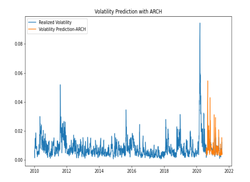
SVM for classification is labeled as Support Vector Classification (SVC). Keeping all characteristics of SVM, it can be applicable to regression. Again, in regression, the aim is to find the hyperplane that minimize the error and maximize the margin. This method is called Support Vector Regression (SVR) and, in this part, we will apply this method to GARCH model. Combining these two models comes up with a different name: SVR-GARCH.

统计代写|机器学习作业代写Machine Learning代考|Neural Network

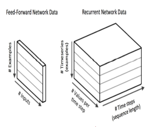
Neural Network (NN) is the building block for deep learning. In NN, data is processed by multiple stages in a way to make a decision. Each neuron takes a result of a dot product as input and use it as input in activation function to make a decision.
$$
z=w_{1} x_{1}+w_{2} x_{2}+b
$$

where $\mathrm{b}$ is bias, $\mathrm{w}$ is weight, and $\mathrm{x}$ is input data.
During this process, input data is undertaken various mathematical manipulation in hidden and output layers. Generally speaking, NN has three types of layers:

• Input layer
• Hidden layer
• Output layer
  Input layer includes raw data. In going from input layer to hidden layer, we learn coefficients. There may be one or more than one hidden layers depending on the network structuree. The more hidden layer the network has, the more complicated it is. Hidden layer, locating between inout and output layers, perform nonlinear transformation via activation function.

Finally, output layer is the layer in which output is produced and decision is made.

In Machine Learning, Gradient Descent is the tool applied to minimize the cost function but employing only gradient descent in neural network is not feasible due to the chain-like structure in neural network. Thus, a new concept known as backpropagation is proposed to minimize the cost function. The idea of backpropagation rest upon the calculating error between observed and actual output and pass this error to the hidden layer. So, we move backward and the main equation takes the form of:
$$
\delta^{l}=\frac{\delta J}{\delta z_{j}^{l}}
$$
where $\mathrm{z}$ is linear transformation and $\delta$ represents error. There is much more to say but to keep myself on track I stop here. For those who wants to dig more into math behind Neural Network please refer to Wilmott (2013) and Alpaydin (2020).

统计代写|机器学习作业代写Machine Learning代考|Bayesian Approach

The way we approach to the probability is of central importance in the sense that it distinquishes the classical (or frequentist) and Bayesian approach.
According to the former method, the relative frequency will converge to the true probability. However, Bayesian application is based on the subjective
interpretation. Unlike frequentists, Bayesian statisticians consider the probability distribution as uncertain and it is revised as new information comes in.
Due to the different interpretation of the probability of these two approaches, likelihood, defined as, given a set of parameters, the probability of observed event, is computed differently.
Starting from joint density function, we can give the mathematical representation of likelihood function:
$$
\mathscr{L}\left(\theta \mid x_{1}, x_{2}, \ldots, x_{p}\right)=\operatorname{Pr}\left(x_{1}, x_{2}, \ldots, x_{p} \mid \theta\right)
$$
Among possible $\theta$ values, what we are trying to do is to decide which one is more likely. Under the statistical model proposed by likelihood function, the observed data $x_{1}, \ldots, x_{p}$ is the most probable.
In fact, you are familiar with the method based on the approach, which is maximum likelihood estimation. Having defined the main difference between Bayesian and Frequentist approaches, it is time to delve more into the Bayes’ Theorem.

机器学习代写

统计代写|机器学习作业代写Machine Learning代考|Support Vector Regression-GARCH

支持向量机 (SVM) 是一种监督学习算法，可适用于分类和回归。SVM 的目标是找到一条分隔两个类的线。这听起来很简单，但这是具有挑战性的部分：几乎可以使用无数条线来区分类别。但是我们正在寻找可以完美区分类别的最佳路线。

在线性代数中，最优直线称为超平面，它使离超平面最近但属于不同类的点之间的距离最大化。两点之间的距离，即支持向量，称为边距。所以，在 SVM 中，我们要做的就是最大化支持向量之间的边距。
用于分类的 SVM 被标记为支持向量分类 (SVC)。保留了 SVM 的所有特性，它可以适用于回归。同样，在回归中，目标是找到最小化误差和最大化边际的超平面。这种方法称为支持向量回归 (SVR)，在这一部分中，我们将把这种方法应用于 GARCH 模型。将这两个模型结合起来就产生了一个不同的名称：SVR-GARCH。

统计代写|机器学习作业代写Machine Learning代考|Neural Network

神经网络 (NN) 是深度学习的基石。在NN中，数据被多个阶段处理以做出决策。每个神经元将点积的结果作为输入，并将其作为激活函数的输入来做出决策。
和=在1X1+在2X2+b

在哪里b是偏见，在是重量，并且X是输入数据。
在此过程中，输入数据在隐藏层和输出层进行各种数学运算。一般来说，NN具有三种类型的层：

• 输入层
• 隐藏层
• 输出层
  输入层包括原始数据。在从输入层到隐藏层的过程中，我们学习系数。取决于网络结构，可能有一个或多个隐藏层。网络的隐藏层越多，它就越复杂。隐藏层，位于输入输出层和输出层之间，通过激活函数执行非线性变换。

最后，输出层是产生输出和做出决策的层。

在机器学习中，梯度下降是用于最小化成本函数的工具，但由于神经网络中的链状结构，仅在神经网络中采用梯度下降是不可行的。因此，提出了一种称为反向传播的新概念来最小化成本函数。反向传播的思想依赖于计算观察到的输出和实际输出之间的误差，并将这个误差传递给隐藏层。因此，我们向后移动，主方程采用以下形式：
d一世=dĴd和j一世
在哪里和是线性变换和d代表错误。还有很多话要说，但为了让自己走上正轨，我在这里停下来。对于那些想要深入了解神经网络背后的数学的人，请参阅 Wilmott (2013) 和 Alpaydin (2020)。

统计代写|机器学习作业代写Machine Learning代考|Bayesian Approach

我们处理概率的方法是至关重要的，因为它区分了经典（或常客）和贝叶斯方法。
根据前一种方法，相对频率会收敛到真实概率。然而，贝叶斯应用是基于主观
解释的。与常客不同，贝叶斯统计学家认为概率分布是不确定的，并且随着新信息的出现而对其进行修改。
由于对这两种方法的概率的不同解释，可能性定义为给定一组参数，观察到的事件的概率, 计算方式不同。
从联合密度函数出发，我们可以给出似然函数的数学表示：
大号(θ∣X1,X2,…,Xp)=公关⁡(X1,X2,…,Xp∣θ)
在可能的θ价值观，我们要做的是决定哪一个更有可能。在似然函数提出的统计模型下，观测数据X1,…,Xp是最有可能的。
其实你很熟悉基于方法的方法，就是最大似然估计。定义了贝叶斯方法和频率方法之间的主要区别之后，是时候深入研究贝叶斯定理了。

统计代写请认准statistics-lab™. statistics-lab™为您的留学生涯保驾护航。统计代写|python代写代考

随机过程代考

在概率论概念中，随机过程是随机变量的集合。 若一随机系统的样本点是随机函数，则称此函数为样本函数，这一随机系统全部样本函数的集合是一个随机过程。 实际应用中，样本函数的一般定义在时间域或者空间域。 随机过程的实例如股票和汇率的波动、语音信号、视频信号、体温的变化，随机运动如布朗运动、随机徘徊等等。

贝叶斯方法代考

贝叶斯统计概念及数据分析表示使用概率陈述回答有关未知参数的研究问题以及统计范式。后验分布包括关于参数的先验分布，和基于观测数据提供关于参数的信息似然模型。根据选择的先验分布和似然模型，后验分布可以解析或近似，例如，马尔科夫链蒙特卡罗 (MCMC) 方法之一。贝叶斯统计概念及数据分析使用后验分布来形成模型参数的各种摘要，包括点估计，如后验平均值、中位数、百分位数和称为可信区间的区间估计。此外，所有关于模型参数的统计检验都可以表示为基于估计后验分布的概率报表。

广义线性模型代考

广义线性模型（GLM）归属统计学领域，是一种应用灵活的线性回归模型。该模型允许因变量的偏差分布有除了正态分布之外的其它分布。

statistics-lab作为专业的留学生服务机构，多年来已为美国、英国、加拿大、澳洲等留学热门地的学生提供专业的学术服务，包括但不限于Essay代写，Assignment代写，Dissertation代写，Report代写，小组作业代写，Proposal代写，Paper代写，Presentation代写，计算机作业代写，论文修改和润色，网课代做，exam代考等等。写作范围涵盖高中，本科，研究生等海外留学全阶段，辐射金融，经济学，会计学，审计学，管理学等全球99%专业科目。写作团队既有专业英语母语作者，也有海外名校硕博留学生，每位写作老师都拥有过硬的语言能力，专业的学科背景和学术写作经验。我们承诺100%原创，100%专业，100%准时，100%满意。

机器学习代写

随着AI的大潮到来，Machine Learning逐渐成为一个新的学习热点。同时与传统CS相比，Machine Learning在其他领域也有着广泛的应用，因此这门学科成为不仅折磨CS专业同学的“小恶魔”，也是折磨生物、化学、统计等其他学科留学生的“大魔王”。学习Machine learning的一大绊脚石在于使用语言众多，跨学科范围广，所以学习起来尤其困难。但是不管你在学习Machine Learning时遇到任何难题，StudyGate专业导师团队都能为你轻松解决。

多元统计分析代考

基础数据: $N$ 个样本， $P$ 个变量数的单样本，组成的横列的数据表
变量定性: 分类和顺序；变量定量：数值
数学公式的角度分为: 因变量与自变量

时间序列分析代写

随机过程，是依赖于参数的一组随机变量的全体，参数通常是时间。 随机变量是随机现象的数量表现，其时间序列是一组按照时间发生先后顺序进行排列的数据点序列。通常一组时间序列的时间间隔为一恒定值（如1秒，5分钟，12小时，7天，1年），因此时间序列可以作为离散时间数据进行分析处理。研究时间序列数据的意义在于现实中，往往需要研究某个事物其随时间发展变化的规律。这就需要通过研究该事物过去发展的历史记录，以得到其自身发展的规律。

回归分析代写

多元回归分析渐进（Multiple Regression Analysis Asymptotics）属于计量经济学领域，主要是一种数学上的统计分析方法，可以分析复杂情况下各影响因素的数学关系，在自然科学、社会和经济学等多个领域内应用广泛。

MATLAB代写

MATLAB 是一种用于技术计算的高性能语言。它将计算、可视化和编程集成在一个易于使用的环境中，其中问题和解决方案以熟悉的数学符号表示。典型用途包括：数学和计算算法开发建模、仿真和原型制作数据分析、探索和可视化科学和工程图形应用程序开发，包括图形用户界面构建MATLAB 是一个交互式系统，其基本数据元素是一个不需要维度的数组。这使您可以解决许多技术计算问题，尤其是那些具有矩阵和向量公式的问题，而只需用 C 或 Fortran 等标量非交互式语言编写程序所需的时间的一小部分。MATLAB 名称代表矩阵实验室。MATLAB 最初的编写目的是提供对由 LINPACK 和 EISPACK 项目开发的矩阵软件的轻松访问，这两个项目共同代表了矩阵计算软件的最新技术。MATLAB 经过多年的发展，得到了许多用户的投入。在大学环境中，它是数学、工程和科学入门和高级课程的标准教学工具。在工业领域，MATLAB 是高效研究、开发和分析的首选工具。MATLAB 具有一系列称为工具箱的特定于应用程序的解决方案。对于大多数 MATLAB 用户来说非常重要，工具箱允许您学习和应用专业技术。工具箱是 MATLAB 函数（M 文件）的综合集合，可扩展 MATLAB 环境以解决特定类别的问题。可用工具箱的领域包括信号处理、控制系统、神经网络、模糊逻辑、小波、仿真等。

R语言代写	问卷设计与分析代写
PYTHON代写	回归分析与线性模型代写
MATLAB代写	方差分析与试验设计代写
STATA代写	机器学习/统计学习代写
SPSS代写	计量经济学代写
EVIEWS代写	时间序列分析代写
EXCEL代写	深度学习代写
SQL代写	各种数据建模与可视化代写

如果你也在 怎样代写机器学习Machine Learning这个学科遇到相关的难题，请随时右上角联系我们的24/7代写客服。

机器学习是人工智能（AI）和计算机科学的一个分支，主要是利用数据和算法来模仿人类的学习方式，逐步提高其准确性。

机器学习是不断增长的数据科学领域的一个重要组成部分。通过使用统计方法，算法被训练来进行分类或预测，在数据挖掘项目中发现关键的洞察力。这些洞察力随后推动了应用程序和业务的决策，最好是影响关键的增长指标。随着大数据的不断扩大和增长，市场对数据科学家的需求将增加，需要他们协助确定最相关的业务问题，随后提供数据来回答这些问题。

statistics-lab™ 为您的留学生涯保驾护航 在代写机器学习Machine Learning方面已经树立了自己的口碑, 保证靠谱, 高质且原创的统计Statistics代写服务。我们的专家在代写机器学习方面经验极为丰富，各种代写机器学习Machine Learning相关的作业也就用不着说。

我们提供的机器学习Machine Learning及其相关学科的代写，服务范围广, 其中包括但不限于:

• Statistical Inference 统计推断
• Statistical Computing 统计计算
• Advanced Probability Theory 高等楖率论
• Advanced Mathematical Statistics 高等数理统计学
• (Generalized) Linear Models 广义线性模型
• Statistical Machine Learning 统计机器学习
• Longitudinal Data Analysis 纵向数据分析
• Foundations of Data Science 数据科学基础

统计代写|机器学习作业代写Machine Learning代考|Machine Learning

“Some concepts are easy to understand but hard to define. This also holds true for volatility” This could be a quote from someone living before Markowitz because the way he model the volatility is very clear and intuitive. Markowitz proposes his celebrated portfolio theory in which volatility is defined as standard deviation so that from then onward finance has become more intertwined with mathematics.

Volatility is the backbone of finance in the sense that it does not only provide information signal to investors but also inputs of various financial models.

What makes volatility so important? The answer stresses the importance of uncertainty, which is the main characteristic of the financial model.

Increased integration of financial markets has led to a prolonged uncertainty in financial market which in turn stresses the importance of volatility, degree at which values of financial assets changes. Volatility has been used as a proxy of risk that in an among the most important variable in many field such as asset pricing and risk management. Its strong presence and latency make it even compulsory to model. Basel Accord, therefore, came into effect in 1996, and volatility as a risk measure has taken the key role in risk management (Karasan and Gaygisiz, 2020).
There is a large and growing body of literature regarding the volatility estimation after the ground-breaking study of Black (1976), Raju and Ghosh (2004), Andersen and Bollerslev (1997), Dokuchaev (2014), and De Stefani et al. (2017). So, we are talking about a long tradition in volatility prediction using ARCH and GARCH-type models in which there are certain drawbacks that might cause failures, e.g., volatility clustering, information asymmetry and so on. Even though, this issues are addressed via differently models, the recent fluctuations in financial markets coupled with the development in machine learning make researchers to rethink volatility estimation.
In this chapter, our aim is to show how we can enhance the predictive performance using machine learning-based model. We will visit various machine learning algorithms, namely support vector regression, neural network, and deep learning, so that we are able to compare the predictive performance.
Modeling volatility amounts to modeling uncertainty so that we better understand and approach the uncertainty enabling us to have good enough approximation to the real world. In order to gauge the extent to which proposed model accounts for the real situation, we need to calculate the return volatility, which is also known as realized volatility. Realized volatility is the square root of realized variance, which is the sum of squared return. Realized volatility is used to calculate the performance of the volatility prediction method. Here is the formula for return volatility:

$$
\hat{\sigma}=\sqrt{\frac{1}{n-1} \sum_{n=1}^{N}\left(r_{n}-\mu\right)^{2}}
$$
where $r$ and $\mu$ are return and mean of return, $n$ is number of observations.

统计代写|机器学习作业代写Machine Learning代考|ARCH Model

One of the early attempt to model the volatility was proposed by Engel (1982) and it is known as ARCH model. ARCH model is a univariate model and it is based on the historical asset returns. The ARCH(p) model has the following form:
$$
\sigma_{t}^{2}=\omega+\sum_{k=1}^{p} \alpha_{k}\left(r_{t-k}\right)^{2}
$$
where
$$
r_{t}=\sigma_{t} \epsilon_{t}
$$
where $\epsilon_{t}$ is assumed to be normally distributed. In this parametric model, we need to satisfy some assumptions to have strictly positive variance. To this respect, following condition should hold:

• $\omega>0$
• $\alpha_{k} \geq 0$
  All these equations tell us that ARCH is a univariate and non-linear model in which volatility is estimated with squared of past returns. The one of the most distinctive feature of $\mathrm{ARCH}$ is that it has the property of the timevarying conditional variance ${ }^{1}$ so that $\mathrm{ARCH}$ is able to model the phenomenon known as volatility clustering, that is large changes tend to be followed by large changes of either sign, and small changes tend to be followed by small changes as put by Benoit Mandelbrot (1963). Hence, once an important announcement arrives into the market, it might results in a huge volatility.

统计代写|机器学习作业代写Machine Learning代考|GARCH Model

GARCH model is an extension of ARCH model incorporating lagged conditional variance. So, ARCH is improved by adding $p$ number of delated conditional variance, which makes GARCH model a multivariate one in the sense that it is a autoregressive moving average models for conditional variance with $\mathrm{p}$ number of lagged squared returns and $\mathrm{q}$ number of lagged conditional variance. GARCH (p, q) can be formulated as:
$$
\sigma_{t}^{2}=\omega+\sum_{k=1}^{q} \alpha_{k} r_{t-k}^{2}+\sum_{k=1}^{p} \beta_{k} \sigma_{t-k}^{2}
$$
where $\omega, \beta$, and $\alpha$ are parameters to be estimated and $\mathrm{q}$ and $\mathrm{p}$ are maximum lag in the model. In order to have consistent GARCH, following conditions
should hold:

• $\omega>0$
• $\beta \geq 0$
• $\alpha \geq 0$
• $\beta+\alpha<1$
  ARCH model is unable to capture the influence of historical innovations. However, as a more parsimonious model, GARCH model can account for the change in historical innovations because GARCH models can be expressed as an infinite-order ARCH. Let’s show how GARCH can be shown as infinite order of ARCH.

机器学习代写

统计代写|机器学习作业代写Machine Learning代考|Machine Learning

“有些概念很容易理解，但很难定义。这也适用于波动率”这可能是生活在 Markowitz 之前的人的一句话，因为他对波动率建模的方式非常清晰和直观。Markowitz 提出了他著名的投资组合理论，其中波动率被定义为标准差，因此从那时起，金融与数学变得更加交织在一起。

从某种意义上说，波动性是金融的支柱，它不仅向投资者提供信息信号，而且还提供各种金融模型的输入。

是什么让波动如此重要？答案强调了不确定性的重要性，这是金融模型的主要特征。

金融市场一体化程度的提高导致金融市场长期存在不确定性，这反过来又强调了波动性的重要性，即金融资产价值变化的程度。波动率已被用作风险的代表，在资产定价和风险管理等许多领域中是最重要的变量之一。它的强大存在和延迟使其甚至强制建模。因此，巴塞尔协议于 1996 年生效，波动性作为一种风险衡量指标在风险管理中发挥了关键作用（Karasan 和 Gaygisiz，2020 年）。
在 Black (1976)、Raju 和 Ghosh (2004)、Andersen 和 Bollerslev (1997)、Dokuchaev (2014) 和 De Stefani 等人的开创性研究之后，关于波动率估计的文献越来越多。（2017）。因此，我们谈论的是使用 ARCH 和 GARCH 型模型进行波动率预测的悠久传统，其中存在可能导致失败的某些缺点，例如波动率聚类、信息不对称等。尽管通过不同的模型解决了这个问题，但最近金融市场的波动以及机器学习的发展使研究人员重新思考波动率估计。
在本章中，我们的目标是展示如何使用基于机器学习的模型来提高预测性能。我们将访问各种机器学习算法，即支持向量回归、神经网络和深度学习，以便我们能够比较预测性能。
对波动性进行建模相当于对不确定性进行建模，以便我们更好地理解和处理不确定性，从而使我们能够对现实世界有足够好的逼近。为了衡量所提出的模型在多大程度上考虑了实际情况，我们需要计算收益波动率，也称为已实现波动率。已实现波动率是已实现方差的平方根，即收益平方和。已实现波动率用于计算波动率预测方法的性能。这是回报波动率的公式：σ^=1n−1∑n=1ñ(rn−μ)2
在哪里r和μ是回报和回报的均值，n是观察次数。

统计代写|机器学习作业代写Machine Learning代考|ARCH Model

Engel (1982) 提出了对波动率建模的早期尝试之一，它被称为 ARCH 模型。ARCH 模型是一个单变量模型，它基于历史资产收益。ARCH(p) 模型具有以下形式：
σ吨2=ω+∑到=1p一种到(r吨−到)2
在哪里
r吨=σ吨ε吨
在哪里ε吨假定为正态分布。在这个参数模型中，我们需要满足一些假设才能具有严格的正方差。对此，应满足以下条件：

• ω>0
• 一种到≥0
  所有这些方程告诉我们，ARCH 是一个单变量和非线性模型，其中波动率是用过去收益的平方来估计的。最显着的特点之一一种RCH是它具有时变条件方差的性质1以便一种RCH能够模拟被称为波动性聚类的现象，即大变化之后往往伴随着任一符号的大变化，而小的变化往往伴随着 Benoit Mandelbrot (1963) 提出的小变化。因此，一旦重要公告进入市场，可能会导致巨大的波动。

统计代写|机器学习作业代写Machine Learning代考|GARCH Model

GARCH 模型是包含滞后条件方差的 ARCH 模型的扩展。因此，通过添加 ARCH 来改进p相关条件方差的数量，这使得 GARCH 模型成为多元模型，因为它是条件方差的自回归移动平均模型p滞后平方收益的数量和q滞后条件方差的数量。GARCH (p, q) 可以表示为：
σ吨2=ω+∑到=1q一种到r吨−到2+∑到=1pb到σ吨−到2
在哪里ω,b， 和一种是要估计的参数和q和p是模型中的最大滞后。为了获得一致的 GARCH，
应满足以下条件：

• ω>0
• b≥0
• 一种≥0
• b+一种<1
  ARCH 模型无法捕捉到历史创新的影响。然而，作为一种更简洁的模型，GARCH 模型可以解释历史创新的变化，因为 GARCH 模型可以表示为无限阶 ARCH。让我们展示如何将 GARCH 显示为 ARCH 的无限阶。

统计代写请认准statistics-lab™. statistics-lab™为您的留学生涯保驾护航。统计代写|python代写代考

随机过程代考

在概率论概念中，随机过程是随机变量的集合。 若一随机系统的样本点是随机函数，则称此函数为样本函数，这一随机系统全部样本函数的集合是一个随机过程。 实际应用中，样本函数的一般定义在时间域或者空间域。 随机过程的实例如股票和汇率的波动、语音信号、视频信号、体温的变化，随机运动如布朗运动、随机徘徊等等。

贝叶斯方法代考

贝叶斯统计概念及数据分析表示使用概率陈述回答有关未知参数的研究问题以及统计范式。后验分布包括关于参数的先验分布，和基于观测数据提供关于参数的信息似然模型。根据选择的先验分布和似然模型，后验分布可以解析或近似，例如，马尔科夫链蒙特卡罗 (MCMC) 方法之一。贝叶斯统计概念及数据分析使用后验分布来形成模型参数的各种摘要，包括点估计，如后验平均值、中位数、百分位数和称为可信区间的区间估计。此外，所有关于模型参数的统计检验都可以表示为基于估计后验分布的概率报表。

广义线性模型代考

广义线性模型（GLM）归属统计学领域，是一种应用灵活的线性回归模型。该模型允许因变量的偏差分布有除了正态分布之外的其它分布。

statistics-lab作为专业的留学生服务机构，多年来已为美国、英国、加拿大、澳洲等留学热门地的学生提供专业的学术服务，包括但不限于Essay代写，Assignment代写，Dissertation代写，Report代写，小组作业代写，Proposal代写，Paper代写，Presentation代写，计算机作业代写，论文修改和润色，网课代做，exam代考等等。写作范围涵盖高中，本科，研究生等海外留学全阶段，辐射金融，经济学，会计学，审计学，管理学等全球99%专业科目。写作团队既有专业英语母语作者，也有海外名校硕博留学生，每位写作老师都拥有过硬的语言能力，专业的学科背景和学术写作经验。我们承诺100%原创，100%专业，100%准时，100%满意。

机器学习代写

随着AI的大潮到来，Machine Learning逐渐成为一个新的学习热点。同时与传统CS相比，Machine Learning在其他领域也有着广泛的应用，因此这门学科成为不仅折磨CS专业同学的“小恶魔”，也是折磨生物、化学、统计等其他学科留学生的“大魔王”。学习Machine learning的一大绊脚石在于使用语言众多，跨学科范围广，所以学习起来尤其困难。但是不管你在学习Machine Learning时遇到任何难题，StudyGate专业导师团队都能为你轻松解决。

多元统计分析代考

基础数据: $N$ 个样本， $P$ 个变量数的单样本，组成的横列的数据表
变量定性: 分类和顺序；变量定量：数值
数学公式的角度分为: 因变量与自变量

时间序列分析代写

随机过程，是依赖于参数的一组随机变量的全体，参数通常是时间。 随机变量是随机现象的数量表现，其时间序列是一组按照时间发生先后顺序进行排列的数据点序列。通常一组时间序列的时间间隔为一恒定值（如1秒，5分钟，12小时，7天，1年），因此时间序列可以作为离散时间数据进行分析处理。研究时间序列数据的意义在于现实中，往往需要研究某个事物其随时间发展变化的规律。这就需要通过研究该事物过去发展的历史记录，以得到其自身发展的规律。

回归分析代写

多元回归分析渐进（Multiple Regression Analysis Asymptotics）属于计量经济学领域，主要是一种数学上的统计分析方法，可以分析复杂情况下各影响因素的数学关系，在自然科学、社会和经济学等多个领域内应用广泛。

MATLAB代写

MATLAB 是一种用于技术计算的高性能语言。它将计算、可视化和编程集成在一个易于使用的环境中，其中问题和解决方案以熟悉的数学符号表示。典型用途包括：数学和计算算法开发建模、仿真和原型制作数据分析、探索和可视化科学和工程图形应用程序开发，包括图形用户界面构建MATLAB 是一个交互式系统，其基本数据元素是一个不需要维度的数组。这使您可以解决许多技术计算问题，尤其是那些具有矩阵和向量公式的问题，而只需用 C 或 Fortran 等标量非交互式语言编写程序所需的时间的一小部分。MATLAB 名称代表矩阵实验室。MATLAB 最初的编写目的是提供对由 LINPACK 和 EISPACK 项目开发的矩阵软件的轻松访问，这两个项目共同代表了矩阵计算软件的最新技术。MATLAB 经过多年的发展，得到了许多用户的投入。在大学环境中，它是数学、工程和科学入门和高级课程的标准教学工具。在工业领域，MATLAB 是高效研究、开发和分析的首选工具。MATLAB 具有一系列称为工具箱的特定于应用程序的解决方案。对于大多数 MATLAB 用户来说非常重要，工具箱允许您学习和应用专业技术。工具箱是 MATLAB 函数（M 文件）的综合集合，可扩展 MATLAB 环境以解决特定类别的问题。可用工具箱的领域包括信号处理、控制系统、神经网络、模糊逻辑、小波、仿真等。

R语言代写	问卷设计与分析代写
PYTHON代写	回归分析与线性模型代写
MATLAB代写	方差分析与试验设计代写
STATA代写	机器学习/统计学习代写
SPSS代写	计量经济学代写
EVIEWS代写	时间序列分析代写
EXCEL代写	深度学习代写
SQL代写	各种数据建模与可视化代写

如果你也在 怎样代写机器学习Machine Learning这个学科遇到相关的难题，请随时右上角联系我们的24/7代写客服。

机器学习是人工智能（AI）和计算机科学的一个分支，主要是利用数据和算法来模仿人类的学习方式，逐步提高其准确性。

机器学习是不断增长的数据科学领域的一个重要组成部分。通过使用统计方法，算法被训练来进行分类或预测，在数据挖掘项目中发现关键的洞察力。这些洞察力随后推动了应用程序和业务的决策，最好是影响关键的增长指标。随着大数据的不断扩大和增长，市场对数据科学家的需求将增加，需要他们协助确定最相关的业务问题，随后提供数据来回答这些问题。

statistics-lab™ 为您的留学生涯保驾护航 在代写机器学习Machine Learning方面已经树立了自己的口碑, 保证靠谱, 高质且原创的统计Statistics代写服务。我们的专家在代写机器学习方面经验极为丰富，各种代写机器学习Machine Learning相关的作业也就用不着说。

我们提供的机器学习Machine Learning及其相关学科的代写，服务范围广, 其中包括但不限于:

• Statistical Inference 统计推断
• Statistical Computing 统计计算
• Advanced Probability Theory 高等楖率论
• Advanced Mathematical Statistics 高等数理统计学
• (Generalized) Linear Models 广义线性模型
• Statistical Machine Learning 统计机器学习
• Longitudinal Data Analysis 纵向数据分析
• Foundations of Data Science 数据科学基础

统计代写|机器学习作业代写Machine Learning代考|Deep Learning

Desp Learning has recently become a buzzword for some good rcasons though the attempt to improve deep learning practices are not the first of it kind. However, it is quite understandable why deep learning has been appreciated for nearly two decades. Deep learning is an abstract concept, which makes it hard to define in a couple of words.

Differently from neural network, deep learning has more complex structure and hidden layers define the complexity. Therefore, some researchers use

number of hidden layer as a comparison benchmark to distinguish the neural network and deep learning, it is useful but not a rigorous way to make this separation. So, a decent definition makes thing clear.
At a high level, deep learning can be defined as:
Deep-learning methods are representation-learningfootnote:
[Representation learning helps us to define a concept in a unique way. For instance, if the task is to detect whether or not it is a circle, then edges play a key role as circle has no edge. So, using color, shape, size, we can create a representation for an object. In essence, this is how human brain works and we know that deep learning structure inspires from the functioning of it.] methods with multiple levels of representation, obtained by composing simple but non-linear modules that each transform the representation at one level (starting with the raw input) into a representation at a higher, slightly more abstract level.
-Le Cunn et al. (2015)
Applications of deep learning dates back to 1940 s in which Cybernetics is published and then Connectivist thinking dominates the years between 1980s and 1990s.Finally, recent development in deep learning such as backpropagation and neural network has created the field as we know as deep learning. Well, basically we are talking about three waves of deep learning and now, it is tempting to ask why deep learning is living its heyday? Goodfellow et al. (2016) list some plausible reasons, which are:

• Increasing Data Sizes
• Increasing Model Sizes
• Increasing Accuracy, Complexity, and Real World Impact
  It seems like modern technology and data availability pave the way for deep learning era in which new data-driven methods are proposed so that we are able to model time series using unconventional models. This development has given rise a new wave of Deep Learning. In Deep Learning, two methods stand out with their ability to include longer time periods: “Recurrent Neural Network” (RNN) and “Long Short-Term Memory” (LSTM).

统计代写|机器学习作业代写Machine Learning代考|Recurrent Neural Network

Recurrent Neural Network has a neural network structure with at least one feedback connection so that network can learn sequences. Feedback connection results in a loop enabling us unveil the non-linear characteristics. This type of connection brings us a new and quite useful property: Memory. Thus, RNN cannot only make use of the input data, but also the previous outputs, which sounds compelling when it comes to time series modeling. RNN comes in many forms such as:

• One-to-One: It consists of single input and single output, which makes it most basic type of RNN.
• One-to-Many: In this form, RNN produces multiple outputs for a single input.
• Many-to-One: As opposed to One-to-Many structure, Many-to-one has multiple inputs for a singly output.
• Many-to-Many: It has multiple outputs and inputs and is known as most complicated structure of RNN.

Hidden unit in RNN feeds itself back into the neural network so that RNN has, unlike feed-forward neural network, recurrent layers, which makes it a suitable method to model a time series data. Therefore, in RNN, activations of a neuron comes from previous time step indication that RNN represents accumulating state of the network instance (Buduma, 2017)
As summarized by Nielsen (2019):

• RNN has time steps one at a time in an orderly fashion.
• The state of the network stays as it is from one time step to another.

统计代写|机器学习作业代写Machine Learning代考|Long-Short Term Memory

Long-Short Term Memory, LSTM for short, deep learning approach has been developed by Hochreiter and Schmidhuber $(1997)$ and it is mainly based on Gated Recurrent Unit (GRU).
GRU is proposed to deal with vanishing gradient problem, which is a common problem in neural network structure and occurs when weight update becomes too small to create a significant change in the network. GRU

consists of two gates: Update and reset. When an early observation is detected as highly important, then we do not update the hidden state. In a similar fashion, when early observations are not significant, it leads to reset the state.

As we previously discussed, the one of the most appealing features of RNN is its ability to connect past and present information. However, this ability turns out to be a failure when “long-term dependencies” comes into the picture. Long-term dependencies mean that model learns from early observations.
For instance, let us examine the following sentence:
Countries have their own currencies as in USA where people transact with dollar

In the case of short-dependencies, it is known that the next predicted word is about a currency but if it is asked which currency is that? Then, things get complicated as we might have various currencies in the text implying longterm dependencies. It is needed to go way back to find something relevant about country using dollar.

LSTM tries to attack the weakness of RNN in long-term dependencies in a way that LSTM has a quite useful tool to get rid of the unnecessary information so that it works more efficiently. LSTM works with gates, enabling LSTM to forget irrelevant data. These are:

• Forget gates
• Input gates
• Output gates
  Forget gates is created to sort out the necessary and unnecessary information so that LSTM performs more efficiently than RNN. In doing so, the value of activation function, sigmoid, becomes zero if the information is irrelevant. Forget gate can be formulated as:
  $$
  F_{t}=\sigma\left(X_{t} W_{I}+h_{t-1} W_{f}+b_{f}\right)
  $$

机器学习代写

统计代写|机器学习作业代写Machine Learning代考|Recurrent Neural Network

循环神经网络具有至少一个反馈连接的神经网络结构，因此网络可以学习序列。反馈连接导致一个循环，使我们能够揭示非线性特性。这种类型的连接为我们带来了一个新的非常有用的属性：内存。因此，RNN 不仅可以利用输入数据，还可以利用之前的输出，这在时间序列建模方面听起来很有吸引力。RNN 有多种形式，例如：

• 一对一：由单输入单输出组成，是RNN的最基本类型。
• 一对多：在这种形式中，RNN 为单个输入生成多个输出。
• 多对一：与一对多结构相反，多对一具有多个输入，用于单个输出。
• 多对多：它有多个输出和输入，被称为RNN最复杂的结构。

RNN 中的隐藏单元将自身反馈到神经网络中，因此与前馈神经网络不同，RNN 具有循环层，这使其成为建模时间序列数据的合适方法。因此，在 RNN 中，神经元的激活来自先前的时间步长指示，表明 RNN 表示网络实例的累积状态 (Buduma, 2017)
正如 Nielsen (2019) 总结的那样：

• RNN 有一个有序的时间步长。
• 从一个时间步到另一个时间步，网络的状态保持不变。

统计代写|机器学习作业代写Machine Learning代考|Long-Short Term Memory

长短期记忆，简称 LSTM，深度学习方法由 Hochreiter 和 Schmidhuber 开发(1997)它主要基于门控循环单元（GRU）。
GRU 被提出来处理消失梯度问题，这是神经网络结构中的一个常见问题，当权重更新变得太小而无法在网络中产生显着变化时会发生。格鲁乌

由两个门组成：更新和重置。当早期观察被检测为非常重要时，我们不会更新隐藏状态。以类似的方式，当早期观察不重要时，它会导致重置状态。

正如我们之前所讨论的，RNN 最吸引人的特性之一是它能够连接过去和现在的信息。然而，当“长期依赖”出现时，这种能力就失败了。长期依赖意味着模型从早期观察中学习。
例如，让我们检查以下句子：
国家有自己的货币，就像美国一样，人们用美元进行交易

在短期依赖的情况下，已知下一个预测词是关于一种货币的，但如果问它是哪种货币？然后，事情变得复杂，因为我们可能在文本中使用各种货币来暗示长期依赖关系。需要回溯到使用美元找到与国家相关的东西。

LSTM 试图攻击 RNN 在长期依赖方面的弱点，LSTM 有一个非常有用的工具来消除不必要的信息，从而使其更有效地工作。LSTM 与门一起工作，使 LSTM 能够忘记不相关的数据。这些都是：

• 忘记大门
• 输入门
• 输出门
  创建遗忘门是为了整理出必要和不必要的信息，以便 LSTM 比 RNN 更有效地执行。在此过程中，如果信息不相关，则激活函数 sigmoid 的值将变为零。遗忘门可以表述为：
  F吨=σ(X吨在一世+H吨−1在F+bF)

统计代写请认准statistics-lab™. statistics-lab™为您的留学生涯保驾护航。统计代写|python代写代考

随机过程代考

在概率论概念中，随机过程是随机变量的集合。 若一随机系统的样本点是随机函数，则称此函数为样本函数，这一随机系统全部样本函数的集合是一个随机过程。 实际应用中，样本函数的一般定义在时间域或者空间域。 随机过程的实例如股票和汇率的波动、语音信号、视频信号、体温的变化，随机运动如布朗运动、随机徘徊等等。

贝叶斯方法代考

贝叶斯统计概念及数据分析表示使用概率陈述回答有关未知参数的研究问题以及统计范式。后验分布包括关于参数的先验分布，和基于观测数据提供关于参数的信息似然模型。根据选择的先验分布和似然模型，后验分布可以解析或近似，例如，马尔科夫链蒙特卡罗 (MCMC) 方法之一。贝叶斯统计概念及数据分析使用后验分布来形成模型参数的各种摘要，包括点估计，如后验平均值、中位数、百分位数和称为可信区间的区间估计。此外，所有关于模型参数的统计检验都可以表示为基于估计后验分布的概率报表。

广义线性模型代考

广义线性模型（GLM）归属统计学领域，是一种应用灵活的线性回归模型。该模型允许因变量的偏差分布有除了正态分布之外的其它分布。

statistics-lab作为专业的留学生服务机构，多年来已为美国、英国、加拿大、澳洲等留学热门地的学生提供专业的学术服务，包括但不限于Essay代写，Assignment代写，Dissertation代写，Report代写，小组作业代写，Proposal代写，Paper代写，Presentation代写，计算机作业代写，论文修改和润色，网课代做，exam代考等等。写作范围涵盖高中，本科，研究生等海外留学全阶段，辐射金融，经济学，会计学，审计学，管理学等全球99%专业科目。写作团队既有专业英语母语作者，也有海外名校硕博留学生，每位写作老师都拥有过硬的语言能力，专业的学科背景和学术写作经验。我们承诺100%原创，100%专业，100%准时，100%满意。

机器学习代写

随着AI的大潮到来，Machine Learning逐渐成为一个新的学习热点。同时与传统CS相比，Machine Learning在其他领域也有着广泛的应用，因此这门学科成为不仅折磨CS专业同学的“小恶魔”，也是折磨生物、化学、统计等其他学科留学生的“大魔王”。学习Machine learning的一大绊脚石在于使用语言众多，跨学科范围广，所以学习起来尤其困难。但是不管你在学习Machine Learning时遇到任何难题，StudyGate专业导师团队都能为你轻松解决。

多元统计分析代考

基础数据: $N$ 个样本， $P$ 个变量数的单样本，组成的横列的数据表
变量定性: 分类和顺序；变量定量：数值
数学公式的角度分为: 因变量与自变量

时间序列分析代写

随机过程，是依赖于参数的一组随机变量的全体，参数通常是时间。 随机变量是随机现象的数量表现，其时间序列是一组按照时间发生先后顺序进行排列的数据点序列。通常一组时间序列的时间间隔为一恒定值（如1秒，5分钟，12小时，7天，1年），因此时间序列可以作为离散时间数据进行分析处理。研究时间序列数据的意义在于现实中，往往需要研究某个事物其随时间发展变化的规律。这就需要通过研究该事物过去发展的历史记录，以得到其自身发展的规律。

回归分析代写

多元回归分析渐进（Multiple Regression Analysis Asymptotics）属于计量经济学领域，主要是一种数学上的统计分析方法，可以分析复杂情况下各影响因素的数学关系，在自然科学、社会和经济学等多个领域内应用广泛。

MATLAB代写

MATLAB 是一种用于技术计算的高性能语言。它将计算、可视化和编程集成在一个易于使用的环境中，其中问题和解决方案以熟悉的数学符号表示。典型用途包括：数学和计算算法开发建模、仿真和原型制作数据分析、探索和可视化科学和工程图形应用程序开发，包括图形用户界面构建MATLAB 是一个交互式系统，其基本数据元素是一个不需要维度的数组。这使您可以解决许多技术计算问题，尤其是那些具有矩阵和向量公式的问题，而只需用 C 或 Fortran 等标量非交互式语言编写程序所需的时间的一小部分。MATLAB 名称代表矩阵实验室。MATLAB 最初的编写目的是提供对由 LINPACK 和 EISPACK 项目开发的矩阵软件的轻松访问，这两个项目共同代表了矩阵计算软件的最新技术。MATLAB 经过多年的发展，得到了许多用户的投入。在大学环境中，它是数学、工程和科学入门和高级课程的标准教学工具。在工业领域，MATLAB 是高效研究、开发和分析的首选工具。MATLAB 具有一系列称为工具箱的特定于应用程序的解决方案。对于大多数 MATLAB 用户来说非常重要，工具箱允许您学习和应用专业技术。工具箱是 MATLAB 函数（M 文件）的综合集合，可扩展 MATLAB 环境以解决特定类别的问题。可用工具箱的领域包括信号处理、控制系统、神经网络、模糊逻辑、小波、仿真等。

R语言代写	问卷设计与分析代写
PYTHON代写	回归分析与线性模型代写
MATLAB代写	方差分析与试验设计代写
STATA代写	机器学习/统计学习代写
SPSS代写	计量经济学代写
EVIEWS代写	时间序列分析代写
EXCEL代写	深度学习代写
SQL代写	各种数据建模与可视化代写

如果你也在 怎样代写机器学习Machine Learning这个学科遇到相关的难题，请随时右上角联系我们的24/7代写客服。

机器学习是人工智能（AI）和计算机科学的一个分支，主要是利用数据和算法来模仿人类的学习方式，逐步提高其准确性。

机器学习是不断增长的数据科学领域的一个重要组成部分。通过使用统计方法，算法被训练来进行分类或预测，在数据挖掘项目中发现关键的洞察力。这些洞察力随后推动了应用程序和业务的决策，最好是影响关键的增长指标。随着大数据的不断扩大和增长，市场对数据科学家的需求将增加，需要他们协助确定最相关的业务问题，随后提供数据来回答这些问题。

statistics-lab™ 为您的留学生涯保驾护航 在代写机器学习Machine Learning方面已经树立了自己的口碑, 保证靠谱, 高质且原创的统计Statistics代写服务。我们的专家在代写机器学习方面经验极为丰富，各种代写机器学习Machine Learning相关的作业也就用不着说。

我们提供的机器学习Machine Learning及其相关学科的代写，服务范围广, 其中包括但不限于:

• Statistical Inference 统计推断
• Statistical Computing 统计计算
• Advanced Probability Theory 高等楖率论
• Advanced Mathematical Statistics 高等数理统计学
• (Generalized) Linear Models 广义线性模型
• Statistical Machine Learning 统计机器学习
• Longitudinal Data Analysis 纵向数据分析
• Foundations of Data Science 数据科学基础

统计代写|机器学习作业代写Machine Learning代考|Autoregressive Model

Dependence structure of succesive terms is the most distinctive feature of the autoregressive model in the sense that current value is regressed over its own lag values in this model. So, we basically forecast the current value of the time series $X_{t}$ by using a linear combination of its past values. Mathematically, the general form of $A R(p)$ can be written as:
$$
X_{t}=c+\alpha_{1} X_{t-1}+\alpha_{2} X_{t-2} \ldots+\alpha_{p} X_{t-p}+\epsilon_{t}
$$
where $\epsilon_{t}$ denotes the residuals and $\mathrm{c}$ is the intercet term. AR(p) model implies that past values up to order $\mathrm{p}$ have somewhat explanatory power on $X_{t}$. If the relationship has shorter memory, then it is likely to model $X_{t}$ with less number of lags.
We have discussed the one of the main properties in time series, which is stationarity and the other important property is invertibility. After introducing

AR model, it is time to show the invertibility of the MA process. It is said to be invertible if it can be converted to infinite AR model.
Differently, under some circumstances, MA can be written as an infinite AR process. These circumstances are to have stationary covariance structure, deterministic part, and invertible MA process. In doing so, we have another model called infinite AR thanks to the assumption of $|\alpha|<1$.
$$
\begin{gathered}
X_{t}=\epsilon_{t}+\alpha \epsilon_{t-1} \
=\epsilon_{t}+\alpha\left(X_{t-1}-\alpha \epsilon_{t-2}\right) \
=\epsilon_{t}+\alpha X_{t-1}-\alpha^{2} \epsilon_{t-2} \
=\epsilon_{t}+\alpha X_{t-1}-\alpha^{2}\left(X_{t-2}+\alpha \epsilon_{t-3}\right) \
\left.=\epsilon_{t}+\alpha X_{t-1}-\alpha^{2} X_{t-2}+\alpha^{3} \epsilon_{t-3}\right) \
=\ldots \
=\alpha X_{t-1}-\alpha^{2} X_{t-2}+\alpha^{3} \epsilon_{t-3}-\alpha^{4} \epsilon_{t-4}+\ldots-(-\alpha)^{n} \epsilon_{t-n}
\end{gathered}
$$
After doing necessary math equation gets the following form:
$$
\alpha^{n} \epsilon_{t-n}=\epsilon_{t}-\sum_{i=0}^{n-1} \alpha^{i} X_{t-i}
$$
In this case, if $|\alpha|<1$. Then $n \rightarrow \infty$
$$
\left.\mathbb{E}\left(\epsilon_{t}-\sum_{i=0}^{n-1} \alpha^{i} X_{t-i}\right)^{2}\right)=\mathbb{E}\left(\alpha^{2 n} \epsilon_{t-n}^{2} \rightarrow \infty\right)
$$
Finally, MA(1) process turns out to be:
$$
\epsilon_{t}=\sum_{i=0}^{\infty} \alpha^{i} X_{t-i}
$$

统计代写|机器学习作业代写Machine Learning代考|Autoregressive Integrated

Autoregressive Integrated Moving Average Model, ARIMA for short, is a function of past values of a time series and white noise. However, ARIMA is proposed as a generalization of AR and MA but they do not have intergration parameter, which helps us to feed model with the raw data. To this respect, even if we include nonstationary data, ARIMA makes it stationary by properly defining the integration parameter.

ARIMA has three parameters, namely p, d, q. As we are familiar from previous time series models $\mathrm{p}$ and $\mathrm{q}$ refer to order of $\mathrm{AR}$ and $\mathrm{MA}$, respectively. But $\mathrm{d}$ controls for level difference. If $\mathrm{d}=1$, it amounts to first difference and if it takes the value of 0 , it means that the model is ARMA.

It is possible to have $\mathrm{d}$ greater than one but it is not as common as having $\mathrm{d}$ of 1 . The ARIMA $(p, 1, q)$ equation has the following structure:
$$
X_{t}=\alpha_{1} d X_{t-1}+\alpha_{2} d X_{t-2} \ldots+\alpha_{p} d X_{t-p}+\epsilon_{t}+\beta_{1} d \epsilon_{t-1}+\beta_{2} d \epsilon_{t-2} \ldots+\beta_{q} d \epsilon_{t-q}
$$
where d refers to difference.
As it is widely embraced and applicable model, Let us discuss the pros and cons of the ARIMA model to get more familiar with the model.
Pros

• ARIMA allows us to work with raw data without considering if it is stationary.
• It performs well with high-frequent data.
• It is less sensitive to the fluctuation in the data compared to other models.
  Cons
• ARIMA might fail in capturing seasonality.
• It work better with a long series and short-term (daily, hourly) data.
• As no automatic updating occurs in ARIMA, no structural break during the analysis period should be observed.
• Having no adjustment in the ARIMA process leads to instability.

统计代写|机器学习作业代写Machine Learning代考|Further Resources

Article cited in this chapter:
Hurvich, Clifford M., and Chih-Ling Tsai. “Regression and time series model selection in small samples.” Biometrika 76 , no. 2 (1989): 297-30.
Books cited in this chapter:

• Buduma, N. and Locascio, N., 2017. Fundamentals of deep learning: Designing next-generation machine intelligence algorithms. O’Reilly Media, Inc.
• Brockwell, Peter J., and Richard A. Davis. Introduction to time series and forecasting. Springer, $2016 .$
• Walsh, Norman, and Leonard Muellner. DocBook: the definitive guide. O’Reilly Media, Inc., $1999 .$

机器学习代写

统计代写|机器学习作业代写Machine Learning代考|Autoregressive Model

连续项的依赖结构是自回归模型最显着的特征，因为当前值在该模型中回归到其自身的滞后值。所以，我们基本上是预测时间序列的当前值X吨通过使用其过去值的线性组合。在数学上，一般形式一种R(p)可以写成：
X吨=C+一种1X吨−1+一种2X吨−2…+一种pX吨−p+ε吨
在哪里ε吨表示残差和C是intercet术语。AR(p) 模型意味着过去的值是有序的p有一定的解释力X吨. 如果关系的记忆较短，那么它很可能建模X吨滞后次数更少。
我们已经讨论了时间序列的一个主要性质，即平稳性，另一个重要性质是可逆性。介绍后

AR模型，是时候展示MA过程的可逆性了。如果可以转化为无限AR模型，就说是可逆的。
不同的是，在某些情况下，MA 可以写成一个无限的 AR 过程。这些情况是具有平稳的协方差结构、确定性部分和可逆的 MA 过程。在这样做的过程中，由于假设|一种|<1.
X吨=ε吨+一种ε吨−1 =ε吨+一种(X吨−1−一种ε吨−2) =ε吨+一种X吨−1−一种2ε吨−2 =ε吨+一种X吨−1−一种2(X吨−2+一种ε吨−3) =ε吨+一种X吨−1−一种2X吨−2+一种3ε吨−3) =… =一种X吨−1−一种2X吨−2+一种3ε吨−3−一种4ε吨−4+…−(−一种)nε吨−n
做必要的数学方程后得到以下形式：
一种nε吨−n=ε吨−∑一世=0n−1一种一世X吨−一世
在这种情况下，如果|一种|<1. 然后n→∞
和(ε吨−∑一世=0n−1一种一世X吨−一世)2)=和(一种2nε吨−n2→∞)
最后，MA(1) 过程变成：
ε吨=∑一世=0∞一种一世X吨−一世

统计代写|机器学习作业代写Machine Learning代考|Autoregressive Integrated

自回归综合移动平均模型，简称 ARIMA，是时间序列过去值和白噪声的函数。然而，ARIMA 被提出作为 AR 和 MA 的推广，但它们没有积分参数，这有助于我们用原始数据提供模型。在这方面，即使我们包含非平稳数据，ARIMA 通过正确定义积分参数使其平稳。

ARIMA有三个参数，即p、d、q。正如我们从以前的时间序列模型中所熟悉的那样p和q参考顺序一种R和米一种， 分别。但d电平差控制。如果d=1, 相当于一阶差分，如果取值为 0 ，则表示模型为 ARMA。

有可能有d大于一，但不如拥有d1 。阿里玛(p,1,q)方程具有以下结构：
X吨=一种1dX吨−1+一种2dX吨−2…+一种pdX吨−p+ε吨+b1dε吨−1+b2dε吨−2…+bqdε吨−q
其中 d 表示差异。
由于它被广泛接受和适用的模型，让我们讨论 ARIMA 模型的优缺点，以更加熟悉该模型。
优点

• ARIMA 允许我们使用原始数据而不考虑它是否是静止的。
• 它在高频数据方面表现良好。
• 与其他模型相比，它对数据的波动不太敏感。
  缺点
• ARIMA 可能无法捕捉季节性。
• 它更适用于长系列和短期（每日、每小时）数据。
• 由于 ARIMA 中不会发生自动更新，因此在分析期间不应观察到结构中断。
• 在 ARIMA 过程中没有调整会导致不稳定。

统计代写|机器学习作业代写Machine Learning代考|Further Resources

本章引用的文章：
Hurvich、Clifford M. 和 Chih-Ling Tsai。“小样本中的回归和时间序列模型选择。” Biometrika 76，没有。2 (1989): 297-30。
本章引用的书籍：

• Buduma, N. 和 Locascio, N.，2017 年。深度学习基础：设计下一代机器智能算法。奥莱利媒体公司
• 布罗克韦尔、彼得 J. 和理查德 A. 戴维斯。时间序列和预测简介。施普林格，2016.
• 沃尔什、诺曼和伦纳德·穆尔纳。DocBook：权威指南。奥莱利媒体公司，1999.

统计代写请认准statistics-lab™. statistics-lab™为您的留学生涯保驾护航。统计代写|python代写代考

随机过程代考

在概率论概念中，随机过程是随机变量的集合。 若一随机系统的样本点是随机函数，则称此函数为样本函数，这一随机系统全部样本函数的集合是一个随机过程。 实际应用中，样本函数的一般定义在时间域或者空间域。 随机过程的实例如股票和汇率的波动、语音信号、视频信号、体温的变化，随机运动如布朗运动、随机徘徊等等。

贝叶斯方法代考

贝叶斯统计概念及数据分析表示使用概率陈述回答有关未知参数的研究问题以及统计范式。后验分布包括关于参数的先验分布，和基于观测数据提供关于参数的信息似然模型。根据选择的先验分布和似然模型，后验分布可以解析或近似，例如，马尔科夫链蒙特卡罗 (MCMC) 方法之一。贝叶斯统计概念及数据分析使用后验分布来形成模型参数的各种摘要，包括点估计，如后验平均值、中位数、百分位数和称为可信区间的区间估计。此外，所有关于模型参数的统计检验都可以表示为基于估计后验分布的概率报表。

广义线性模型代考

广义线性模型（GLM）归属统计学领域，是一种应用灵活的线性回归模型。该模型允许因变量的偏差分布有除了正态分布之外的其它分布。

statistics-lab作为专业的留学生服务机构，多年来已为美国、英国、加拿大、澳洲等留学热门地的学生提供专业的学术服务，包括但不限于Essay代写，Assignment代写，Dissertation代写，Report代写，小组作业代写，Proposal代写，Paper代写，Presentation代写，计算机作业代写，论文修改和润色，网课代做，exam代考等等。写作范围涵盖高中，本科，研究生等海外留学全阶段，辐射金融，经济学，会计学，审计学，管理学等全球99%专业科目。写作团队既有专业英语母语作者，也有海外名校硕博留学生，每位写作老师都拥有过硬的语言能力，专业的学科背景和学术写作经验。我们承诺100%原创，100%专业，100%准时，100%满意。

机器学习代写

随着AI的大潮到来，Machine Learning逐渐成为一个新的学习热点。同时与传统CS相比，Machine Learning在其他领域也有着广泛的应用，因此这门学科成为不仅折磨CS专业同学的“小恶魔”，也是折磨生物、化学、统计等其他学科留学生的“大魔王”。学习Machine learning的一大绊脚石在于使用语言众多，跨学科范围广，所以学习起来尤其困难。但是不管你在学习Machine Learning时遇到任何难题，StudyGate专业导师团队都能为你轻松解决。

多元统计分析代考

基础数据: $N$ 个样本， $P$ 个变量数的单样本，组成的横列的数据表
变量定性: 分类和顺序；变量定量：数值
数学公式的角度分为: 因变量与自变量

时间序列分析代写

随机过程，是依赖于参数的一组随机变量的全体，参数通常是时间。 随机变量是随机现象的数量表现，其时间序列是一组按照时间发生先后顺序进行排列的数据点序列。通常一组时间序列的时间间隔为一恒定值（如1秒，5分钟，12小时，7天，1年），因此时间序列可以作为离散时间数据进行分析处理。研究时间序列数据的意义在于现实中，往往需要研究某个事物其随时间发展变化的规律。这就需要通过研究该事物过去发展的历史记录，以得到其自身发展的规律。

回归分析代写

多元回归分析渐进（Multiple Regression Analysis Asymptotics）属于计量经济学领域，主要是一种数学上的统计分析方法，可以分析复杂情况下各影响因素的数学关系，在自然科学、社会和经济学等多个领域内应用广泛。

MATLAB代写

MATLAB 是一种用于技术计算的高性能语言。它将计算、可视化和编程集成在一个易于使用的环境中，其中问题和解决方案以熟悉的数学符号表示。典型用途包括：数学和计算算法开发建模、仿真和原型制作数据分析、探索和可视化科学和工程图形应用程序开发，包括图形用户界面构建MATLAB 是一个交互式系统，其基本数据元素是一个不需要维度的数组。这使您可以解决许多技术计算问题，尤其是那些具有矩阵和向量公式的问题，而只需用 C 或 Fortran 等标量非交互式语言编写程序所需的时间的一小部分。MATLAB 名称代表矩阵实验室。MATLAB 最初的编写目的是提供对由 LINPACK 和 EISPACK 项目开发的矩阵软件的轻松访问，这两个项目共同代表了矩阵计算软件的最新技术。MATLAB 经过多年的发展，得到了许多用户的投入。在大学环境中，它是数学、工程和科学入门和高级课程的标准教学工具。在工业领域，MATLAB 是高效研究、开发和分析的首选工具。MATLAB 具有一系列称为工具箱的特定于应用程序的解决方案。对于大多数 MATLAB 用户来说非常重要，工具箱允许您学习和应用专业技术。工具箱是 MATLAB 函数（M 文件）的综合集合，可扩展 MATLAB 环境以解决特定类别的问题。可用工具箱的领域包括信号处理、控制系统、神经网络、模糊逻辑、小波、仿真等。

R语言代写	问卷设计与分析代写
PYTHON代写	回归分析与线性模型代写
MATLAB代写	方差分析与试验设计代写
STATA代写	机器学习/统计学习代写
SPSS代写	计量经济学代写
EVIEWS代写	时间序列分析代写
EXCEL代写	深度学习代写
SQL代写	各种数据建模与可视化代写

如果你也在 怎样代写机器学习Machine Learning这个学科遇到相关的难题，请随时右上角联系我们的24/7代写客服。

机器学习是人工智能（AI）和计算机科学的一个分支，主要是利用数据和算法来模仿人类的学习方式，逐步提高其准确性。

机器学习是不断增长的数据科学领域的一个重要组成部分。通过使用统计方法，算法被训练来进行分类或预测，在数据挖掘项目中发现关键的洞察力。这些洞察力随后推动了应用程序和业务的决策，最好是影响关键的增长指标。随着大数据的不断扩大和增长，市场对数据科学家的需求将增加，需要他们协助确定最相关的业务问题，随后提供数据来回答这些问题。

statistics-lab™ 为您的留学生涯保驾护航 在代写机器学习Machine Learning方面已经树立了自己的口碑, 保证靠谱, 高质且原创的统计Statistics代写服务。我们的专家在代写机器学习方面经验极为丰富，各种代写机器学习Machine Learning相关的作业也就用不着说。

我们提供的机器学习Machine Learning及其相关学科的代写，服务范围广, 其中包括但不限于:

• Statistical Inference 统计推断
• Statistical Computing 统计计算
• Advanced Probability Theory 高等楖率论
• Advanced Mathematical Statistics 高等数理统计学
• (Generalized) Linear Models 广义线性模型
• Statistical Machine Learning 统计机器学习
• Longitudinal Data Analysis 纵向数据分析
• Foundations of Data Science 数据科学基础

统计代写|机器学习作业代写Machine Learning代考|Series Modeling

Some models account better for some phenomena, certain approaches capture the characteristics of an event in a solid way. Time series modeling is a vivid example for this because vast majority of financial data have time dimension, which makes time series applications a necessary tool for finance. In simple terms, the ordering of the data and correlation among them is of importance.
In this chapter of the book, classical time series models will be discussed and the performance of these models will be compared. On top of that, the deep learning based time series analysis will be introduced in the [Link to Come], which has entirely different approach in terms of data preparation and model structure. The classical models to be visited include moving average model (MA), autoregressive model (AR), and finally autoregressive integrated moving average

model (ARIMA). What is common across these models are the information carried by the historical observations. If these historical observations are obtained from error terms, it is referred to as moving average, if these observations come out of time series itself, it turns out to be autoregressive. The other model, namely ARIMA, is an extension of these models.
Here is a formal definition of time series:
A time series is a set of observations $X_{t}$, each one being recorded at a specific time t. A discrete-time time series (the type to which this book is primarily devoted) is one in which the set $T_{0}$ of times at which observations are made is a discrete set, as is the case, for example, when observations are made at fixed time intervals. Contintuous time series are obtained when observations are recorded continuously over some time interval.
-Brockwell and Davis (2016)
Let us observe what data with time dimension looks like. Figure 2-1 exhibits the oil prices for the period of $1980-2020$ and the following Python code shows us a way of producing this plot.

统计代写|机器学习作业代写Machine Learning代考|Residual

Residual is known as irregular component of time series. Technically speaking, residual is equal to the difference between observations and related fitted values. So, we can think of it as a left over from the model.

As we have discussed before time series models lack in some core assumptions but it does not necessarily mean that time series models are free from assumptions. I would like to stress the most prominents one, which is called stationarity.
Stationarity means that statistical properties such as mean, variance, and covariance of the time series do not change over time.
There are two forms of stationarity:
1) Weak Stationarity: Time series, $X_{t}$, is said to be stationarity if

• $X_{t}$ has finite variance, $\mathbb{E}\left(X_{t}^{2}\right)<\infty, \forall t \in \mathbb{Z}$
• Mean value of $X_{t}$ is constant and does solely depend on time, $\mathbb{E}\left(X_{t}\right)=\mu, t \forall \in \mathbb{Z}$
• Covariance structure, $\gamma(t, t+h)$, depends on the time difference only: $\gamma(h)=\gamma_{h}+\gamma(t+h, t)$
  In words, time series should have finite variance with constant mean, and covariance structure that is a function of time difference.

2) Strong Stationarity: If the joint distribution of $X_{t 1}, X_{t 2}, \ldots X_{t k}$ is the same with the shifted version of set $X_{t 1+h}, X_{t 2+h}, \ldots X_{t k+h}$, it is referred to as strong stationarity. Thus, strong stationarity implies that distribution of random variable of a random process is the same with shifting time index.
The question is now why do we need stationarity? The reason is two fold.
First, in the estimation process, it is essential to have some distribution as time goes on. In other words, if distribution of a time series change over time, it becomes unpredictable and cannot be modeled.

The ultimate aim of time series models is forecasting. To do that we should estimate the coefficients first, which corresponds to learning in Machine Learning. Once we learn and conduct forecasting analysis, we assume that the distribution of the data in estimation stays the same in a way that we have the same estimated coefficients. If this is not the case, we should re-estimate the coefficients because we are unable to to forecast with the previous estimated coefficients.

统计代写|机器学习作业代写Machine Learning代考|Cyclicality

What if data does not show fixed period movements? At this point, cyclicality comes into the picture. It exists when higher periodic variation than the trend emerges. Some confuse cyclicality and seasonality in a sense that they both exhibit expansion and contraction. We can, however, think of cyclicality as business cycles, which takes a long time to complete its cycle and the ups and downs over a long horizon. So, cyclicality is different from seasonality in the sense that there is no fluctuation in a fixed period. An example for cyclicality may be the house purchases (or sales) depending on mortgage rate. That is, when a mortgage rate is cut (or raise), it leads to a boost for house purchase (or sales).

机器学习代写

统计代写|机器学习作业代写Machine Learning代考|Series Modeling

有些模型更好地解释了某些现象，某些方法以可靠的方式捕捉了事件的特征。时间序列建模就是一个生动的例子，因为绝大多数金融数据都有时间维度，这使得时间序列应用成为金融的必要工具。简单来说，数据的排序和它们之间的相关性很重要。
在本书的这一章中，将讨论经典的时间序列模型并比较这些模型的性能。最重要的是，基于深度学习的时间序列分析将在[Link to Come]中介绍，在数据准备和模型结构方面有完全不同的方法。要访问的经典模型包括移动平均模型（MA），自回归模型（AR），最后是自回归综合移动平均

模型（ARIMA）。这些模型的共同点是历史观察所携带的信息。如果这些历史观察是从误差项中获得的，则称为移动平均线，如果这些观察来自时间序列本身，则结果是自回归的。另一个模型，即 ARIMA，是这些模型的扩展。
这是时间序列的正式定义：
时间序列是一组观察值X吨，每一个都是在特定的时间 t 记录的。离散时间序列（本书主要介绍的类型）是一个集合吨0进行观察的时间是一个离散集，例如，当以固定的时间间隔进行观察时。当观测值在某个时间间隔内连续记录时，就获得了连续的时间序列。
-Brockwell and Davis (2016)
让我们观察具有时间维度的数据是什么样的。图 2-1 显示了 2019 年的油价1980−2020下面的 Python 代码向我们展示了一种生成此图的方法。

统计代写|机器学习作业代写Machine Learning代考|Residual

残差被称为时间序列的不规则分量。从技术上讲，残差等于观测值与相关拟合值之间的差异。因此，我们可以将其视为模型的遗留物。

正如我们之前讨论过的，时间序列模型缺乏一些核心假设，但这并不一定意味着时间序列模型没有假设。我想强调最突出的一个，这就是所谓的平稳性。
平稳性意味着时间序列的均值、方差和协方差等统计属性不会随时间变化。
平稳性有两种形式：
1）弱平稳性：时间序列，X吨, 据说是平稳的，如果

• X吨具有有限方差，和(X吨2)<∞,∀吨∈从
• 的平均值X吨是恒定的并且完全取决于时间，和(X吨)=μ,吨∀∈从
• 协方差结构，C(吨,吨+H)，仅取决于时差：C(H)=CH+C(吨+H,吨)
  换句话说，时间序列应该具有具有恒定均值的有限方差，以及作为时间差函数的协方差结构。

2）强平稳性：如果联合分布X吨1,X吨2,…X吨到与 set 的移位版本相同X吨1+H,X吨2+H,…X吨到+H，称为强平稳性。因此，强平稳性意味着随机过程的随机变量分布与移动时间指数相同。
现在的问题是为什么我们需要平稳性？原因有两个。
首先，在估计过程中，随着时间的推移有一定的分布是必不可少的。换句话说，如果时间序列的分布随时间变化，它就会变得不可预测并且无法建模。

时间序列模型的最终目的是预测。为此，我们应该首先估计系数，这对应于机器学习中的学习。一旦我们学习并进行了预测分析，我们假设估计中的数据分布保持不变，因为我们有相同的估计系数。如果不是这种情况，我们应该重新估计系数，因为我们无法用以前估计的系数进行预测。

统计代写|机器学习作业代写Machine Learning代考|Cyclicality

如果数据没有显示固定期间的变动怎么办？在这一点上，周期性出现了。当出现比趋势更高的周期性变化时，它就存在。有些人混淆了周期性和季节性，因为它们都表现出扩张和收缩。然而，我们可以将周期性视为商业周期，它需要很长时间才能完成其周期以及长期的起伏。因此，周期性不同于季节性，因为在固定时期内没有波动。周期性的一个例子可能是取决于抵押贷款利率的房屋购买（或销售）。也就是说，当抵押贷款利率降低（或提高）时，会促进购房（或销售）。

统计代写请认准statistics-lab™. statistics-lab™为您的留学生涯保驾护航。统计代写|python代写代考

随机过程代考

在概率论概念中，随机过程是随机变量的集合。 若一随机系统的样本点是随机函数，则称此函数为样本函数，这一随机系统全部样本函数的集合是一个随机过程。 实际应用中，样本函数的一般定义在时间域或者空间域。 随机过程的实例如股票和汇率的波动、语音信号、视频信号、体温的变化，随机运动如布朗运动、随机徘徊等等。

贝叶斯方法代考

贝叶斯统计概念及数据分析表示使用概率陈述回答有关未知参数的研究问题以及统计范式。后验分布包括关于参数的先验分布，和基于观测数据提供关于参数的信息似然模型。根据选择的先验分布和似然模型，后验分布可以解析或近似，例如，马尔科夫链蒙特卡罗 (MCMC) 方法之一。贝叶斯统计概念及数据分析使用后验分布来形成模型参数的各种摘要，包括点估计，如后验平均值、中位数、百分位数和称为可信区间的区间估计。此外，所有关于模型参数的统计检验都可以表示为基于估计后验分布的概率报表。

广义线性模型代考

广义线性模型（GLM）归属统计学领域，是一种应用灵活的线性回归模型。该模型允许因变量的偏差分布有除了正态分布之外的其它分布。

statistics-lab作为专业的留学生服务机构，多年来已为美国、英国、加拿大、澳洲等留学热门地的学生提供专业的学术服务，包括但不限于Essay代写，Assignment代写，Dissertation代写，Report代写，小组作业代写，Proposal代写，Paper代写，Presentation代写，计算机作业代写，论文修改和润色，网课代做，exam代考等等。写作范围涵盖高中，本科，研究生等海外留学全阶段，辐射金融，经济学，会计学，审计学，管理学等全球99%专业科目。写作团队既有专业英语母语作者，也有海外名校硕博留学生，每位写作老师都拥有过硬的语言能力，专业的学科背景和学术写作经验。我们承诺100%原创，100%专业，100%准时，100%满意。

机器学习代写

随着AI的大潮到来，Machine Learning逐渐成为一个新的学习热点。同时与传统CS相比，Machine Learning在其他领域也有着广泛的应用，因此这门学科成为不仅折磨CS专业同学的“小恶魔”，也是折磨生物、化学、统计等其他学科留学生的“大魔王”。学习Machine learning的一大绊脚石在于使用语言众多，跨学科范围广，所以学习起来尤其困难。但是不管你在学习Machine Learning时遇到任何难题，StudyGate专业导师团队都能为你轻松解决。

多元统计分析代考

基础数据: $N$ 个样本， $P$ 个变量数的单样本，组成的横列的数据表
变量定性: 分类和顺序；变量定量：数值
数学公式的角度分为: 因变量与自变量

时间序列分析代写

随机过程，是依赖于参数的一组随机变量的全体，参数通常是时间。 随机变量是随机现象的数量表现，其时间序列是一组按照时间发生先后顺序进行排列的数据点序列。通常一组时间序列的时间间隔为一恒定值（如1秒，5分钟，12小时，7天，1年），因此时间序列可以作为离散时间数据进行分析处理。研究时间序列数据的意义在于现实中，往往需要研究某个事物其随时间发展变化的规律。这就需要通过研究该事物过去发展的历史记录，以得到其自身发展的规律。

回归分析代写

多元回归分析渐进（Multiple Regression Analysis Asymptotics）属于计量经济学领域，主要是一种数学上的统计分析方法，可以分析复杂情况下各影响因素的数学关系，在自然科学、社会和经济学等多个领域内应用广泛。

MATLAB代写

MATLAB 是一种用于技术计算的高性能语言。它将计算、可视化和编程集成在一个易于使用的环境中，其中问题和解决方案以熟悉的数学符号表示。典型用途包括：数学和计算算法开发建模、仿真和原型制作数据分析、探索和可视化科学和工程图形应用程序开发，包括图形用户界面构建MATLAB 是一个交互式系统，其基本数据元素是一个不需要维度的数组。这使您可以解决许多技术计算问题，尤其是那些具有矩阵和向量公式的问题，而只需用 C 或 Fortran 等标量非交互式语言编写程序所需的时间的一小部分。MATLAB 名称代表矩阵实验室。MATLAB 最初的编写目的是提供对由 LINPACK 和 EISPACK 项目开发的矩阵软件的轻松访问，这两个项目共同代表了矩阵计算软件的最新技术。MATLAB 经过多年的发展，得到了许多用户的投入。在大学环境中，它是数学、工程和科学入门和高级课程的标准教学工具。在工业领域，MATLAB 是高效研究、开发和分析的首选工具。MATLAB 具有一系列称为工具箱的特定于应用程序的解决方案。对于大多数 MATLAB 用户来说非常重要，工具箱允许您学习和应用专业技术。工具箱是 MATLAB 函数（M 文件）的综合集合，可扩展 MATLAB 环境以解决特定类别的问题。可用工具箱的领域包括信号处理、控制系统、神经网络、模糊逻辑、小波、仿真等。

R语言代写	问卷设计与分析代写
PYTHON代写	回归分析与线性模型代写
MATLAB代写	方差分析与试验设计代写
STATA代写	机器学习/统计学习代写
SPSS代写	计量经济学代写
EVIEWS代写	时间序列分析代写
EXCEL代写	深度学习代写
SQL代写	各种数据建模与可视化代写

如果你也在 怎样代写机器学习Machine Learning这个学科遇到相关的难题，请随时右上角联系我们的24/7代写客服。

机器学习是人工智能（AI）和计算机科学的一个分支，主要是利用数据和算法来模仿人类的学习方式，逐步提高其准确性。

机器学习是不断增长的数据科学领域的一个重要组成部分。通过使用统计方法，算法被训练来进行分类或预测，在数据挖掘项目中发现关键的洞察力。这些洞察力随后推动了应用程序和业务的决策，最好是影响关键的增长指标。随着大数据的不断扩大和增长，市场对数据科学家的需求将增加，需要他们协助确定最相关的业务问题，随后提供数据来回答这些问题。

statistics-lab™ 为您的留学生涯保驾护航 在代写机器学习Machine Learning方面已经树立了自己的口碑, 保证靠谱, 高质且原创的统计Statistics代写服务。我们的专家在代写机器学习方面经验极为丰富，各种代写机器学习Machine Learning相关的作业也就用不着说。

我们提供的机器学习Machine Learning及其相关学科的代写，服务范围广, 其中包括但不限于:

• Statistical Inference 统计推断
• Statistical Computing 统计计算
• Advanced Probability Theory 高等楖率论
• Advanced Mathematical Statistics 高等数理统计学
• (Generalized) Linear Models 广义线性模型
• Statistical Machine Learning 统计机器学习
• Longitudinal Data Analysis 纵向数据分析
• Foundations of Data Science 数据科学基础

统计代写|机器学习作业代写Machine Learning代考|Financial Risk Management

Though it is theoretically intuitive, the assumption of completely rational decision maker, main building block in modern finance theory, is too perfect to be real. This idea, therefore, attacked by behavioral economists, who believes that psychology plays a key role in decision making process.
Making decisions is like speaking prose – people do it all the time, knowingly or unknowingly. It is hardly surprising, then, that the topic of decision making is shared by many disciplines, from mathematics and statistics, through economics and political science, to sociology and psychology.
-Kahneman and Tversky (1984)
Information asymmetry and financial risk management goes hand in hand as cost of financing and firm valuation are deeply affected by the information asymmetry. That is, uncertainty in valuation of a firm’s assets might raise the borrowing cost posing a threat to a firm’s sustainability (See DeMarzo and Darrell (1995) and Froot, Scharfstein, and Stein (1993)).

Thus, roots of the failures described above lie deeper in such a way that perfect hypothetical world in which rational decision maker lives is unable to explain them. At this point, human instincts and imperfect world come into play and a mixture of disciplines provide more plausible justifications. So, it turns out Adverse Selection and Moral Hazard are two prominents categories accounting for the market failures.

统计代写|机器学习作业代写Machine Learning代考|Adverse Selection

It is a type of asymmetric information in which one party tries to exploit its informational advantage. Adverse selection arises when seller are better informed than buyers. This phemomenon is perfectly coined by Akerlof $(1970)$ as “The Markets for Lemons”. Within this framework, lemons refer to low-quality.

Consider a market with lemon and high-quality cars and buyers know that it is likely to buy a lemon, which lowers then equilibrium price. However, seller is better informed if the car is lemon or high-quality. So, in this situation, benefit from exchange might disappear and no transaction takes place.
Due to the complexity and opaqueness, mortgage market in the pre-crisis era is a good example of adverse selection. More elaborately, borrowers knew more about their willingness and ability to pay than lenders. Financial risk was created through the securitizations of the loans, i.e., mortgage backed securities. From this point on, the originators of the mortgage loans knew more about the risks than the people they were selling them to investors in the mortgage backed securities.

Let us try to model adverse selection using Python. It is readily observable in insurance industry and therefore I would like to focus on this industry to model adverse selection.
Supposc that the consumer utility function is:
$$
U(x)=e^{\gamma x}
$$
where $\mathrm{x}$ is income and $\gamma$ is a parameter, which takes on values between 0 and $1 .$

The ultimate aim of this example is to decide whether or not to buy an insurance based on consumer utility.
For the sake of practice, I assume that the income is $\$ 2 \mathrm{USD}$ and cost of the accident is \$1.5 USD.

Now it is time to calculate the probability of loss, $\pi$, which is exogenously given and it is uniformly distributed.
As a last step, in order to find equilibrium, I have to define supply and demand for insurance coverage. The following code block indicates how we can model the adverse selection.

统计代写|机器学习作业代写Machine Learning代考|Moral Hazard

Market failures also result from asymmetric information. In moral hazard situation, one party of the contract assumes more risk than the other party. Formally, moral hazard may be defined as a situation in which more informed party takes advantages of the private information at his disposal to the detriment of others.

For a better understanding of moral hazard, a simple example can be given from the credit market: Suppose that entity A demands credit for use in financing the project, which is considered as feasible to finance. Moral hazurd arises if entity A utilizes the loan for the payment of oredit debt to bank $\mathrm{C}$, without prior notice to the lender bank. While allocating credit, the moral hazard situation that banks may encounter arises as a result of asymmetric information, decreases banks’ lending appetites and appears as one of the reasons why banks put so much labor on credit allocation process.
Some argue that rescue operation undertaken by FED for LCTM can be considered as moral hazard in a way that FED enters into contracts on bad faith.

机器学习代写

统计代写|机器学习作业代写Machine Learning代考|Financial Risk Management

尽管在理论上是直观的，但完全理性决策者的假设，现代金融理论的主要组成部分，过于完美而无法实现。因此，这一想法受到行为经济学家的攻击，他们认为心理学在决策过程中起着关键作用。
做决定就像说散文——人们一直在做，有意或无意。因此，从数学和统计学到经济学和政治学，再到社会学和心理学，许多学科都共享决策这一主题也就不足为奇了。
——卡尼曼和特沃斯基（1984）
信息不对称与财务风险管理齐头并进，因为信息不对称对融资成本和公司估值的影响很大。也就是说，公司资产估值的不确定性可能会提高借贷成本，从而对公司的可持续性构成威胁（参见 DeMarzo 和 Darrell (1995) 以及 Froot、Scharfstein 和 Stein (1993)）。

因此，上述失败的根源更深，以至于理性决策者生活的完美假设世界无法解释它们。在这一点上，人类的本能和不完美的世界开始发挥作用，学科的混合提供了更合理的理由。因此，事实证明逆向选择和道德风险是导致市场失灵的两个突出类别。

统计代写|机器学习作业代写Machine Learning代考|Adverse Selection

它是一种不对称信息，其中一方试图利用其信息优势。当卖方比买方更了解情况时，就会出现逆向选择。这种现象完全由阿克洛夫创造(1970)作为“柠檬市场”。在这个框架内，柠檬指的是低质量的。

考虑一个有柠檬和高质量汽车的市场，买家知道它可能会购买柠檬，这会降低均衡价格。但是，如果汽车是柠檬车还是优质车，卖家会更好地了解情况。因此，在这种情况下，从交换中获得的收益可能会消失，并且不会发生交易。
由于复杂性和不透明性，危机前时代的抵押贷款市场是逆向选择的一个很好的例子。更详细地说，借款人比贷款人更了解他们的支付意愿和能力。金融风险是通过贷款证券化（即抵押支持证券）产生的。从那时起，抵押贷款的发起人比他们向抵押贷款支持证券的投资者出售贷款的人更了解风险。

让我们尝试使用 Python 对逆向选择进行建模。它在保险行业很容易观察到，因此我想专注于这个行业来模拟逆向选择。
假设消费者效用函数为：
ü(X)=和CX
在哪里X是收入和C是一个参数，取值介于 0 和1.

这个例子的最终目的是根据消费者效用决定是否购买保险。
为了实践起见，我假设收入是$2ü小号D事故费用为1.5 美元。

现在是计算损失概率的时候了，圆周率，它是外生给定的，并且是均匀分布的。
作为最后一步，为了找到平衡，我必须定义保险范围的供需。以下代码块指示我们如何对逆向选择进行建模。

统计代写|机器学习作业代写Machine Learning代考|Moral Hazard

市场失灵也源于信息不对称。在道德风险情况下，合同一方承担的风险大于另一方。形式上，道德风险可以定义为更知情的一方利用他掌握的私人信息损害他人的情况。

为了更好地理解道德风险，可以从信贷市场举一个简单的例子：假设实体 A 需要信贷来为项目融资，这被认为是可行的。如果实体 A 将贷款用于向银行支付或编辑债务，则会出现道德风险C，无需事先通知贷方银行。在信贷配置过程中，由于信息不对称，银行可能遇到的道德风险情况，降低了银行的放贷意愿，成为银行在信贷配置过程中投入大量精力的原因之一。
一些人认为，美联储为 LCTM 采取的救援行动可以被视为道德风险，因为美联储在签订合同时是出于恶意。

统计代写请认准statistics-lab™. statistics-lab™为您的留学生涯保驾护航。统计代写|python代写代考

随机过程代考

在概率论概念中，随机过程是随机变量的集合。 若一随机系统的样本点是随机函数，则称此函数为样本函数，这一随机系统全部样本函数的集合是一个随机过程。 实际应用中，样本函数的一般定义在时间域或者空间域。 随机过程的实例如股票和汇率的波动、语音信号、视频信号、体温的变化，随机运动如布朗运动、随机徘徊等等。

贝叶斯方法代考

贝叶斯统计概念及数据分析表示使用概率陈述回答有关未知参数的研究问题以及统计范式。后验分布包括关于参数的先验分布，和基于观测数据提供关于参数的信息似然模型。根据选择的先验分布和似然模型，后验分布可以解析或近似，例如，马尔科夫链蒙特卡罗 (MCMC) 方法之一。贝叶斯统计概念及数据分析使用后验分布来形成模型参数的各种摘要，包括点估计，如后验平均值、中位数、百分位数和称为可信区间的区间估计。此外，所有关于模型参数的统计检验都可以表示为基于估计后验分布的概率报表。

广义线性模型代考

广义线性模型（GLM）归属统计学领域，是一种应用灵活的线性回归模型。该模型允许因变量的偏差分布有除了正态分布之外的其它分布。

statistics-lab作为专业的留学生服务机构，多年来已为美国、英国、加拿大、澳洲等留学热门地的学生提供专业的学术服务，包括但不限于Essay代写，Assignment代写，Dissertation代写，Report代写，小组作业代写，Proposal代写，Paper代写，Presentation代写，计算机作业代写，论文修改和润色，网课代做，exam代考等等。写作范围涵盖高中，本科，研究生等海外留学全阶段，辐射金融，经济学，会计学，审计学，管理学等全球99%专业科目。写作团队既有专业英语母语作者，也有海外名校硕博留学生，每位写作老师都拥有过硬的语言能力，专业的学科背景和学术写作经验。我们承诺100%原创，100%专业，100%准时，100%满意。

机器学习代写

随着AI的大潮到来，Machine Learning逐渐成为一个新的学习热点。同时与传统CS相比，Machine Learning在其他领域也有着广泛的应用，因此这门学科成为不仅折磨CS专业同学的“小恶魔”，也是折磨生物、化学、统计等其他学科留学生的“大魔王”。学习Machine learning的一大绊脚石在于使用语言众多，跨学科范围广，所以学习起来尤其困难。但是不管你在学习Machine Learning时遇到任何难题，StudyGate专业导师团队都能为你轻松解决。

多元统计分析代考

基础数据: $N$ 个样本， $P$ 个变量数的单样本，组成的横列的数据表
变量定性: 分类和顺序；变量定量：数值
数学公式的角度分为: 因变量与自变量

时间序列分析代写

随机过程，是依赖于参数的一组随机变量的全体，参数通常是时间。 随机变量是随机现象的数量表现，其时间序列是一组按照时间发生先后顺序进行排列的数据点序列。通常一组时间序列的时间间隔为一恒定值（如1秒，5分钟，12小时，7天，1年），因此时间序列可以作为离散时间数据进行分析处理。研究时间序列数据的意义在于现实中，往往需要研究某个事物其随时间发展变化的规律。这就需要通过研究该事物过去发展的历史记录，以得到其自身发展的规律。

回归分析代写

多元回归分析渐进（Multiple Regression Analysis Asymptotics）属于计量经济学领域，主要是一种数学上的统计分析方法，可以分析复杂情况下各影响因素的数学关系，在自然科学、社会和经济学等多个领域内应用广泛。

MATLAB代写

MATLAB 是一种用于技术计算的高性能语言。它将计算、可视化和编程集成在一个易于使用的环境中，其中问题和解决方案以熟悉的数学符号表示。典型用途包括：数学和计算算法开发建模、仿真和原型制作数据分析、探索和可视化科学和工程图形应用程序开发，包括图形用户界面构建MATLAB 是一个交互式系统，其基本数据元素是一个不需要维度的数组。这使您可以解决许多技术计算问题，尤其是那些具有矩阵和向量公式的问题，而只需用 C 或 Fortran 等标量非交互式语言编写程序所需的时间的一小部分。MATLAB 名称代表矩阵实验室。MATLAB 最初的编写目的是提供对由 LINPACK 和 EISPACK 项目开发的矩阵软件的轻松访问，这两个项目共同代表了矩阵计算软件的最新技术。MATLAB 经过多年的发展，得到了许多用户的投入。在大学环境中，它是数学、工程和科学入门和高级课程的标准教学工具。在工业领域，MATLAB 是高效研究、开发和分析的首选工具。MATLAB 具有一系列称为工具箱的特定于应用程序的解决方案。对于大多数 MATLAB 用户来说非常重要，工具箱允许您学习和应用专业技术。工具箱是 MATLAB 函数（M 文件）的综合集合，可扩展 MATLAB 环境以解决特定类别的问题。可用工具箱的领域包括信号处理、控制系统、神经网络、模糊逻辑、小波、仿真等。

R语言代写	问卷设计与分析代写
PYTHON代写	回归分析与线性模型代写
MATLAB代写	方差分析与试验设计代写
STATA代写	机器学习/统计学习代写
SPSS代写	计量经济学代写
EVIEWS代写	时间序列分析代写
EXCEL代写	深度学习代写
SQL代写	各种数据建模与可视化代写

如果你也在 怎样代写机器学习Machine Learning这个学科遇到相关的难题，请随时右上角联系我们的24/7代写客服。

机器学习是人工智能（AI）和计算机科学的一个分支，主要是利用数据和算法来模仿人类的学习方式，逐步提高其准确性。

机器学习是不断增长的数据科学领域的一个重要组成部分。通过使用统计方法，算法被训练来进行分类或预测，在数据挖掘项目中发现关键的洞察力。这些洞察力随后推动了应用程序和业务的决策，最好是影响关键的增长指标。随着大数据的不断扩大和增长，市场对数据科学家的需求将增加，需要他们协助确定最相关的业务问题，随后提供数据来回答这些问题。

statistics-lab™ 为您的留学生涯保驾护航 在代写机器学习Machine Learning方面已经树立了自己的口碑, 保证靠谱, 高质且原创的统计Statistics代写服务。我们的专家在代写机器学习方面经验极为丰富，各种代写机器学习Machine Learning相关的作业也就用不着说。

我们提供的机器学习Machine Learning及其相关学科的代写，服务范围广, 其中包括但不限于:

• Statistical Inference 统计推断
• Statistical Computing 统计计算
• Advanced Probability Theory 高等楖率论
• Advanced Mathematical Statistics 高等数理统计学
• (Generalized) Linear Models 广义线性模型
• Statistical Machine Learning 统计机器学习
• Longitudinal Data Analysis 纵向数据分析
• Foundations of Data Science 数据科学基础

统计代写|机器学习作业代写Machine Learning代考|Fundamentals of Risk Management

In 2007, no one would have thought that risk functions could have changed as much as they have in the last eight years. It is a natural temptation to expect that the next decade has to contain less change. However, we believe that the opposite will likely be true.
-Harle et al. (2016)
Risk management is a constantly evolving process. Constant evolution is inevitable due to the fact that long-standing risk management practice cannot keep pace with recent development or be a precursor of unfolding crises. Therefore, it is of importance to monitor and adopt the changes brought by structural breaks in a risk management process. Adoption to the changes implies re-defining the components and tools of risk management and this is what this book is all about.

Traditionally, in finance, empirical research in finance has a strong focus on statistical inference. Econometric has been built upon the rationale of

statistical inference. These types of models concentrate on the structure of underlying data generating process and relationship among variables.
Machine learning models, however, are not assumed to define the underlying data generating process but are considered as a means to an end for the purpose of prediction (Lommers et al. 2021). Thus, machine learning models are tend to be more data-centric and prediction accuracy-oriented.
Moreover, data scarcity and unavailability has always been an issue in finance and it is not hard to guess that the econometric models cannot perform well in this case. Given the solution of machine learning models to the data unavailability via synthetic data generation, machine learning models has been on the top of the agenda in finance and financial risk management is, of course, no exception.
Before going into the detail and discuss these tools, it is worth introducing the main risk management concepts. Thus, this part of the book presents basic concepts of financial risk management, which I will refer throughout the book. These concepts include risk, types of risks, risk management, returns, and some concepts related to risk management.

统计代写|机器学习作业代写Machine Learning代考|All financial investments

All financial investments are undertaken to gain profit, which is also called return. More formally, return is the gain made on an investment in a given period of time. Thus, return refers to the upside of the risk. Throughout the book, risk and return will refer to downside and upside risk, respectively.
As you can imagine, there is a trade-off between risk and return, the higher risk assumed, the greater the return realized. As it is a formidable task to come up with a optimum solution, this trade-off is one of the most controversial issues in finance. However, Markowitz (1952) proposes an intuitive and appealing solution to this long-standing issue. The way he defined risk, which was until then ambiguous, is nice and clean and led to a shift in landscape in financial research. Markowitz (1952) used standard deviation $\sigma_{R_{i}}$ to quantify risk. This intuitive definition allows researchers to use mathematics and statistics in finance. The standard deviation can be mathematically defined as (Hull, 2012):
$$
\sigma=\sqrt{\mathbb{E}\left(R^{2}\right)-[\mathbb{E}(R)]^{2}}
$$
where $\mathrm{R}$ and $\mathbb{E}$ symbols refer to annual return and expectation, respectively. The book uses the symbol $\mathbb{E}$ numerous times as expected return represent the return of interest. This is because it is probability we are talking about in defining risk. When it comes to portfolio variance, covariance comes into the picture and the formula turns out to be:

$$
\sigma_{p}^{2}=w_{a}^{2} \sigma_{a}^{2}+w_{b}^{2} \sigma_{b}^{2}+2 w_{a} w_{b} \operatorname{Cov}\left(r_{a}, r_{b}\right)
$$
where w denotes weight, $\sigma^{2}$ is variance, and $\operatorname{Cov}$ is covariance matrix. Taking square root of the variance obtained above gives us the portfolio standard deviation:
$$
\sigma_{p}=\sqrt{\sigma_{p}^{2}}
$$
In other words, portfolio expected return is a weighted average of the individual returns and can be shown as:
$$
\mathbb{E}(R)=\sum_{i}^{n} w_{i} R_{i}=w_{1} R_{1}+w_{2} R_{2} \cdots+w_{n} R_{n}
$$
Let us explore the risk-return relationship by visualization. To do that, an hypothetical portfolio is constructed to calculate necessary statistics with Python.

统计代写|机器学习作业代写Machine Learning代考|Risk Management

Financial risk management is a process to deal with the uncertainties resulting from financial markets. It involves assessing the financial risks facing an organization and developing management strategies consistent with internal priorities and policies (Horcher, 2011).
According to this definition, as every organization faces different type of risks, the way that a company deals with it is completely unique. Every company should properly assess and take necessary action against risk. It, however, does not necessarily mean that once a risk is identified, it needs to be mitigated as much as a company can do.
Risk management is, therefore, not about mitigating risk at all costs. Mitigating risk may require sacrificing return and it can be tolerable up to certain level as companies are searching for higher return as much as lowering risk. Thus, to maximize profit while lowering the risk should be delicate and well-defined task.

Managing risk is a delicate task as it comes with a cost and even though dealing with it requires specific company policies, there exists a general framework for possible risk strategies. These are:

• Ignore: In this strategy, companies accept all risks and their consequences and prefer to do nothing.
• Transfer: This strategy involves transferring the risks to a thirdparty by hedging or some other ways.
• Mitigate: Companies develop a strategy to mitigate risk partly because its harmful effect might be considered too much to bear and/or supprass the benefit attached to it.
• Accept risk: If companies embrace the strategy of accepting the risk, they properly identify risks and acknowledge the benefit of them. In other words, when assuming certain risks arising from some activities bring values to shareholder, this strategy can be picked.

机器学习代写

统计代写|机器学习作业代写Machine Learning代考|Fundamentals of Risk Management

在 2007 年，没有人会想到风险职能会发生像过去八年那样大的变化。期望下一个十年必须包含更少的变化是一种自然的诱惑。然而，我们认为情况可能正好相反。
-Harle 等人。(2016)
风险管理是一个不断发展的过程。由于长期的风险管理实践无法跟上最近的发展步伐或成为危机蔓延的前兆，因此不断演变是不可避免的。因此，在风险管理过程中监控和采用结构性中断带来的变化非常重要。采用这些变化意味着重新定义风险管理的组件和工具，这就是本书的全部内容。

传统上，在金融领域，金融领域的实证研究非常关注统计推断。计量经济学建立在以下基本原理之上

统计推断。这些类型的模型专注于底层数据生成过程的结构和变量之间的关系。
然而，机器学习模型并未被假定为定义基础数据生成过程，而是被视为达到预测目的的一种手段（Lommers 等人，2021 年）。因此，机器学习模型往往更加以数据为中心和以预测准确性为导向。
此外，数据稀缺和不可用一直是金融领域的一个问题，不难猜测，计量经济学模型在这种情况下表现不佳。鉴于机器学习模型通过合成数据生成来解决数据不可用的问题，机器学习模型一直是金融领域的首要任务，金融风险管理当然也不例外。
在深入讨论这些工具之前，有必要介绍一下主要的风险管理概念。因此，本书的这一部分介绍了金融风险管理的基本概念，我将在整本书中提及这些概念。这些概念包括风险、风险类型、风险管理、收益以及与风险管理相关的一些概念。

统计代写|机器学习作业代写Machine Learning代考|All financial investments

所有的金融投资都是为了获得利润，也叫回报。更正式地说，回报是在给定时间段内投资所获得的收益。因此，回报是指风险的上升。在整本书中，风险和回报将分别指下行风险和上行风险。
可以想象，风险和回报之间存在权衡，承担的风险越高，实现的回报就越大。由于提出最佳解决方案是一项艰巨的任务，因此这种权衡是金融界最具争议的问题之一。然而，Markowitz (1952) 为这个长期存在的问题提出了一个直观且有吸引力的解决方案。他定义风险的方式，在此之前是模棱两可的，但它很好而且很干净，并导致了金融研究领域的转变。Markowitz (1952) 使用标准差 $\sigma_{R_{i}}$ 来量化风险。这个直观的定义允许研究人员在金融中使用数学和统计学。标准差可以在数学上定义为 (Hull, 2012)：
$$
\sigma=\sqrt{\mathbb{E}\left(R^{2}\right)-[\mathbb{E}(​​R)]^ {2}}
$$
其中 $\mathrm{R}$ 和 $\mathbb{E}$ 符号分别表示年回报率和期望值。本书多次使用符号$\mathbb{E}$，因为预期回报代表利息回报。这是因为我们在定义风险时谈论的是概率。当谈到投资组合方差时，协方差就出现了，公式结果是：

$$
\sigma_{p}^{2}=w_{a}^{2} \sigma_{a}^{2}+w_{b}^{2} \sigma_{b}^{2}+2 w_ {a} w_{b} \operatorname{Cov}\left(r_{a}, r_{b}\right)
$$
其中 w 表示权重，$\sigma^{2}$ 是方差，$\operatorname{ Cov}$ 是协方差矩阵。取上面获得的方差的平方根，我们得到了投资组合标准差：
$$
\sigma_{p}=\sqrt{\sigma_{p}^{2}}
$$
换句话说，投资组合预期收益是个人的回报可以表示为：
$$
\mathbb{E}(​​R)=\sum_{i}^{n} w_{i} R_{i}=w_{1} R_{1}+w_{2 } R_{2} \cdots+w_{n} R_{n}
$$
让我们通过可视化来探索风险回报关系。为此，构建了一个假设的投资组合以使用 Python 计算必要的统计数据。

统计代写|机器学习作业代写Machine Learning代考|Risk Management

金融风险管理是应对金融市场带来的不确定性的过程。它涉及评估组织面临的财务风险并制定与内部优先事项和政策一致的管理战略（Horcher，2011 年）。
根据这个定义，由于每个组织都面临不同类型的风险，因此公司处理风险的方式是完全不同的。每家公司都应正确评估风险并采取必要的措施来应对风险。然而，这并不一定意味着一旦确定了风险，就需要尽可能地减轻风险。
因此，风险管理并不是不惜一切代价降低风险。降低风险可能需要牺牲回报，并且在一定程度上是可以容忍的，因为公司正在寻求更高的回报以及降低风险。因此，在降低风险的同时最大化利润应该是一项微妙而明确的任务。

管理风险是一项微妙的任务，因为它伴随着成本，尽管处理它需要特定的公司政策，但存在可能的风险策略的一般框架。这些都是：

• 忽略：在这种策略中，公司接受所有风险及其后果，宁愿什么也不做。
• 转移：该策略涉及通过对冲或其他方式将风险转移给第三方。
• 缓解：公司制定降低风险的战略，部分原因是其有害影响可能被认为太多，无法承担和/或超过它所带来的好处。
• 接受风险：如果公司采用接受风险的策略，他们就会正确识别风险并承认风险的好处。换句话说，当假设某些活动产生的某些风险为股东带来价值时，可以选择这种策略。

统计代写请认准statistics-lab™. statistics-lab™为您的留学生涯保驾护航。统计代写|python代写代考

随机过程代考

在概率论概念中，随机过程是随机变量的集合。 若一随机系统的样本点是随机函数，则称此函数为样本函数，这一随机系统全部样本函数的集合是一个随机过程。 实际应用中，样本函数的一般定义在时间域或者空间域。 随机过程的实例如股票和汇率的波动、语音信号、视频信号、体温的变化，随机运动如布朗运动、随机徘徊等等。

贝叶斯方法代考

贝叶斯统计概念及数据分析表示使用概率陈述回答有关未知参数的研究问题以及统计范式。后验分布包括关于参数的先验分布，和基于观测数据提供关于参数的信息似然模型。根据选择的先验分布和似然模型，后验分布可以解析或近似，例如，马尔科夫链蒙特卡罗 (MCMC) 方法之一。贝叶斯统计概念及数据分析使用后验分布来形成模型参数的各种摘要，包括点估计，如后验平均值、中位数、百分位数和称为可信区间的区间估计。此外，所有关于模型参数的统计检验都可以表示为基于估计后验分布的概率报表。

广义线性模型代考

广义线性模型（GLM）归属统计学领域，是一种应用灵活的线性回归模型。该模型允许因变量的偏差分布有除了正态分布之外的其它分布。

statistics-lab作为专业的留学生服务机构，多年来已为美国、英国、加拿大、澳洲等留学热门地的学生提供专业的学术服务，包括但不限于Essay代写，Assignment代写，Dissertation代写，Report代写，小组作业代写，Proposal代写，Paper代写，Presentation代写，计算机作业代写，论文修改和润色，网课代做，exam代考等等。写作范围涵盖高中，本科，研究生等海外留学全阶段，辐射金融，经济学，会计学，审计学，管理学等全球99%专业科目。写作团队既有专业英语母语作者，也有海外名校硕博留学生，每位写作老师都拥有过硬的语言能力，专业的学科背景和学术写作经验。我们承诺100%原创，100%专业，100%准时，100%满意。

机器学习代写

随着AI的大潮到来，Machine Learning逐渐成为一个新的学习热点。同时与传统CS相比，Machine Learning在其他领域也有着广泛的应用，因此这门学科成为不仅折磨CS专业同学的“小恶魔”，也是折磨生物、化学、统计等其他学科留学生的“大魔王”。学习Machine learning的一大绊脚石在于使用语言众多，跨学科范围广，所以学习起来尤其困难。但是不管你在学习Machine Learning时遇到任何难题，StudyGate专业导师团队都能为你轻松解决。

多元统计分析代考

基础数据: $N$ 个样本， $P$ 个变量数的单样本，组成的横列的数据表
变量定性: 分类和顺序；变量定量：数值
数学公式的角度分为: 因变量与自变量

时间序列分析代写

随机过程，是依赖于参数的一组随机变量的全体，参数通常是时间。 随机变量是随机现象的数量表现，其时间序列是一组按照时间发生先后顺序进行排列的数据点序列。通常一组时间序列的时间间隔为一恒定值（如1秒，5分钟，12小时，7天，1年），因此时间序列可以作为离散时间数据进行分析处理。研究时间序列数据的意义在于现实中，往往需要研究某个事物其随时间发展变化的规律。这就需要通过研究该事物过去发展的历史记录，以得到其自身发展的规律。

回归分析代写

多元回归分析渐进（Multiple Regression Analysis Asymptotics）属于计量经济学领域，主要是一种数学上的统计分析方法，可以分析复杂情况下各影响因素的数学关系，在自然科学、社会和经济学等多个领域内应用广泛。

MATLAB代写

MATLAB 是一种用于技术计算的高性能语言。它将计算、可视化和编程集成在一个易于使用的环境中，其中问题和解决方案以熟悉的数学符号表示。典型用途包括：数学和计算算法开发建模、仿真和原型制作数据分析、探索和可视化科学和工程图形应用程序开发，包括图形用户界面构建MATLAB 是一个交互式系统，其基本数据元素是一个不需要维度的数组。这使您可以解决许多技术计算问题，尤其是那些具有矩阵和向量公式的问题，而只需用 C 或 Fortran 等标量非交互式语言编写程序所需的时间的一小部分。MATLAB 名称代表矩阵实验室。MATLAB 最初的编写目的是提供对由 LINPACK 和 EISPACK 项目开发的矩阵软件的轻松访问，这两个项目共同代表了矩阵计算软件的最新技术。MATLAB 经过多年的发展，得到了许多用户的投入。在大学环境中，它是数学、工程和科学入门和高级课程的标准教学工具。在工业领域，MATLAB 是高效研究、开发和分析的首选工具。MATLAB 具有一系列称为工具箱的特定于应用程序的解决方案。对于大多数 MATLAB 用户来说非常重要，工具箱允许您学习和应用专业技术。工具箱是 MATLAB 函数（M 文件）的综合集合，可扩展 MATLAB 环境以解决特定类别的问题。可用工具箱的领域包括信号处理、控制系统、神经网络、模糊逻辑、小波、仿真等。

R语言代写	问卷设计与分析代写
PYTHON代写	回归分析与线性模型代写
MATLAB代写	方差分析与试验设计代写
STATA代写	机器学习/统计学习代写
SPSS代写	计量经济学代写
EVIEWS代写	时间序列分析代写
EXCEL代写	深度学习代写
SQL代写	各种数据建模与可视化代写