如果你也在 怎样代写机器学习Machine Learning这个学科遇到相关的难题,请随时右上角联系我们的24/7代写客服。
机器学习是人工智能(AI)和计算机科学的一个分支,主要是利用数据和算法来模仿人类的学习方式,逐步提高其准确性。
机器学习是不断增长的数据科学领域的一个重要组成部分。通过使用统计方法,算法被训练来进行分类或预测,在数据挖掘项目中发现关键的洞察力。这些洞察力随后推动了应用程序和业务的决策,最好是影响关键的增长指标。随着大数据的不断扩大和增长,市场对数据科学家的需求将增加,需要他们协助确定最相关的业务问题,随后提供数据来回答这些问题。
statistics-lab™ 为您的留学生涯保驾护航 在代写机器学习Machine Learning方面已经树立了自己的口碑, 保证靠谱, 高质且原创的统计Statistics代写服务。我们的专家在代写机器学习方面经验极为丰富,各种代写机器学习Machine Learning相关的作业也就用不着说。
我们提供的机器学习Machine Learning及其相关学科的代写,服务范围广, 其中包括但不限于:
- Statistical Inference 统计推断
- Statistical Computing 统计计算
- Advanced Probability Theory 高等楖率论
- Advanced Mathematical Statistics 高等数理统计学
- (Generalized) Linear Models 广义线性模型
- Statistical Machine Learning 统计机器学习
- Longitudinal Data Analysis 纵向数据分析
- Foundations of Data Science 数据科学基础
统计代写|机器学习作业代写Machine Learning代考|Series Modeling
Some models account better for some phenomena, certain approaches capture the characteristics of an event in a solid way. Time series modeling is a vivid example for this because vast majority of financial data have time dimension, which makes time series applications a necessary tool for finance. In simple terms, the ordering of the data and correlation among them is of importance.
In this chapter of the book, classical time series models will be discussed and the performance of these models will be compared. On top of that, the deep learning based time series analysis will be introduced in the [Link to Come], which has entirely different approach in terms of data preparation and model structure. The classical models to be visited include moving average model (MA), autoregressive model (AR), and finally autoregressive integrated moving average
model (ARIMA). What is common across these models are the information carried by the historical observations. If these historical observations are obtained from error terms, it is referred to as moving average, if these observations come out of time series itself, it turns out to be autoregressive. The other model, namely ARIMA, is an extension of these models.
Here is a formal definition of time series:
A time series is a set of observations $X_{t}$, each one being recorded at a specific time t. A discrete-time time series (the type to which this book is primarily devoted) is one in which the set $T_{0}$ of times at which observations are made is a discrete set, as is the case, for example, when observations are made at fixed time intervals. Contintuous time series are obtained when observations are recorded continuously over some time interval.
-Brockwell and Davis (2016)
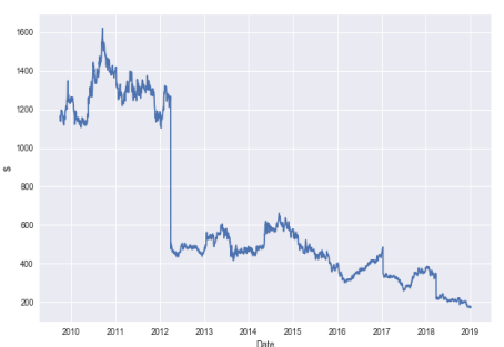
Let us observe what data with time dimension looks like. Figure 2-1 exhibits the oil prices for the period of $1980-2020$ and the following Python code shows us a way of producing this plot.
统计代写|机器学习作业代写Machine Learning代考|Residual
Residual is known as irregular component of time series. Technically speaking, residual is equal to the difference between observations and related fitted values. So, we can think of it as a left over from the model.
As we have discussed before time series models lack in some core assumptions but it does not necessarily mean that time series models are free from assumptions. I would like to stress the most prominents one, which is called stationarity.
Stationarity means that statistical properties such as mean, variance, and covariance of the time series do not change over time.
There are two forms of stationarity:
1) Weak Stationarity: Time series, $X_{t}$, is said to be stationarity if
- $X_{t}$ has finite variance, $\mathbb{E}\left(X_{t}^{2}\right)<\infty, \forall t \in \mathbb{Z}$
- Mean value of $X_{t}$ is constant and does solely depend on time, $\mathbb{E}\left(X_{t}\right)=\mu, t \forall \in \mathbb{Z}$
- Covariance structure, $\gamma(t, t+h)$, depends on the time difference only: $\gamma(h)=\gamma_{h}+\gamma(t+h, t)$
In words, time series should have finite variance with constant mean, and covariance structure that is a function of time difference.
2) Strong Stationarity: If the joint distribution of $X_{t 1}, X_{t 2}, \ldots X_{t k}$ is the same with the shifted version of set $X_{t 1+h}, X_{t 2+h}, \ldots X_{t k+h}$, it is referred to as strong stationarity. Thus, strong stationarity implies that distribution of random variable of a random process is the same with shifting time index.
The question is now why do we need stationarity? The reason is two fold.
First, in the estimation process, it is essential to have some distribution as time goes on. In other words, if distribution of a time series change over time, it becomes unpredictable and cannot be modeled.
The ultimate aim of time series models is forecasting. To do that we should estimate the coefficients first, which corresponds to learning in Machine Learning. Once we learn and conduct forecasting analysis, we assume that the distribution of the data in estimation stays the same in a way that we have the same estimated coefficients. If this is not the case, we should re-estimate the coefficients because we are unable to to forecast with the previous estimated coefficients.
统计代写|机器学习作业代写Machine Learning代考|Cyclicality
What if data does not show fixed period movements? At this point, cyclicality comes into the picture. It exists when higher periodic variation than the trend emerges. Some confuse cyclicality and seasonality in a sense that they both exhibit expansion and contraction. We can, however, think of cyclicality as business cycles, which takes a long time to complete its cycle and the ups and downs over a long horizon. So, cyclicality is different from seasonality in the sense that there is no fluctuation in a fixed period. An example for cyclicality may be the house purchases (or sales) depending on mortgage rate. That is, when a mortgage rate is cut (or raise), it leads to a boost for house purchase (or sales).
机器学习代写
统计代写|机器学习作业代写Machine Learning代考|Series Modeling
有些模型更好地解释了某些现象,某些方法以可靠的方式捕捉了事件的特征。时间序列建模就是一个生动的例子,因为绝大多数金融数据都有时间维度,这使得时间序列应用成为金融的必要工具。简单来说,数据的排序和它们之间的相关性很重要。
在本书的这一章中,将讨论经典的时间序列模型并比较这些模型的性能。最重要的是,基于深度学习的时间序列分析将在[Link to Come]中介绍,在数据准备和模型结构方面有完全不同的方法。要访问的经典模型包括移动平均模型(MA),自回归模型(AR),最后是自回归综合移动平均
模型(ARIMA)。这些模型的共同点是历史观察所携带的信息。如果这些历史观察是从误差项中获得的,则称为移动平均线,如果这些观察来自时间序列本身,则结果是自回归的。另一个模型,即 ARIMA,是这些模型的扩展。
这是时间序列的正式定义:
时间序列是一组观察值X吨,每一个都是在特定的时间 t 记录的。离散时间序列(本书主要介绍的类型)是一个集合吨0进行观察的时间是一个离散集,例如,当以固定的时间间隔进行观察时。当观测值在某个时间间隔内连续记录时,就获得了连续的时间序列。
-Brockwell and Davis (2016)
让我们观察具有时间维度的数据是什么样的。图 2-1 显示了 2019 年的油价1980−2020下面的 Python 代码向我们展示了一种生成此图的方法。
统计代写|机器学习作业代写Machine Learning代考|Residual
残差被称为时间序列的不规则分量。从技术上讲,残差等于观测值与相关拟合值之间的差异。因此,我们可以将其视为模型的遗留物。
正如我们之前讨论过的,时间序列模型缺乏一些核心假设,但这并不一定意味着时间序列模型没有假设。我想强调最突出的一个,这就是所谓的平稳性。
平稳性意味着时间序列的均值、方差和协方差等统计属性不会随时间变化。
平稳性有两种形式:
1)弱平稳性:时间序列,X吨, 据说是平稳的,如果
- X吨具有有限方差,和(X吨2)<∞,∀吨∈从
- 的平均值X吨是恒定的并且完全取决于时间,和(X吨)=μ,吨∀∈从
- 协方差结构,C(吨,吨+H),仅取决于时差:C(H)=CH+C(吨+H,吨)
换句话说,时间序列应该具有具有恒定均值的有限方差,以及作为时间差函数的协方差结构。
2)强平稳性:如果联合分布X吨1,X吨2,…X吨到与 set 的移位版本相同X吨1+H,X吨2+H,…X吨到+H,称为强平稳性。因此,强平稳性意味着随机过程的随机变量分布与移动时间指数相同。
现在的问题是为什么我们需要平稳性?原因有两个。
首先,在估计过程中,随着时间的推移有一定的分布是必不可少的。换句话说,如果时间序列的分布随时间变化,它就会变得不可预测并且无法建模。
时间序列模型的最终目的是预测。为此,我们应该首先估计系数,这对应于机器学习中的学习。一旦我们学习并进行了预测分析,我们假设估计中的数据分布保持不变,因为我们有相同的估计系数。如果不是这种情况,我们应该重新估计系数,因为我们无法用以前估计的系数进行预测。
统计代写|机器学习作业代写Machine Learning代考|Cyclicality
如果数据没有显示固定期间的变动怎么办?在这一点上,周期性出现了。当出现比趋势更高的周期性变化时,它就存在。有些人混淆了周期性和季节性,因为它们都表现出扩张和收缩。然而,我们可以将周期性视为商业周期,它需要很长时间才能完成其周期以及长期的起伏。因此,周期性不同于季节性,因为在固定时期内没有波动。周期性的一个例子可能是取决于抵押贷款利率的房屋购买(或销售)。也就是说,当抵押贷款利率降低(或提高)时,会促进购房(或销售)。

统计代写请认准statistics-lab™. statistics-lab™为您的留学生涯保驾护航。统计代写|python代写代考
随机过程代考
在概率论概念中,随机过程是随机变量的集合。 若一随机系统的样本点是随机函数,则称此函数为样本函数,这一随机系统全部样本函数的集合是一个随机过程。 实际应用中,样本函数的一般定义在时间域或者空间域。 随机过程的实例如股票和汇率的波动、语音信号、视频信号、体温的变化,随机运动如布朗运动、随机徘徊等等。
贝叶斯方法代考
贝叶斯统计概念及数据分析表示使用概率陈述回答有关未知参数的研究问题以及统计范式。后验分布包括关于参数的先验分布,和基于观测数据提供关于参数的信息似然模型。根据选择的先验分布和似然模型,后验分布可以解析或近似,例如,马尔科夫链蒙特卡罗 (MCMC) 方法之一。贝叶斯统计概念及数据分析使用后验分布来形成模型参数的各种摘要,包括点估计,如后验平均值、中位数、百分位数和称为可信区间的区间估计。此外,所有关于模型参数的统计检验都可以表示为基于估计后验分布的概率报表。
广义线性模型代考
广义线性模型(GLM)归属统计学领域,是一种应用灵活的线性回归模型。该模型允许因变量的偏差分布有除了正态分布之外的其它分布。
statistics-lab作为专业的留学生服务机构,多年来已为美国、英国、加拿大、澳洲等留学热门地的学生提供专业的学术服务,包括但不限于Essay代写,Assignment代写,Dissertation代写,Report代写,小组作业代写,Proposal代写,Paper代写,Presentation代写,计算机作业代写,论文修改和润色,网课代做,exam代考等等。写作范围涵盖高中,本科,研究生等海外留学全阶段,辐射金融,经济学,会计学,审计学,管理学等全球99%专业科目。写作团队既有专业英语母语作者,也有海外名校硕博留学生,每位写作老师都拥有过硬的语言能力,专业的学科背景和学术写作经验。我们承诺100%原创,100%专业,100%准时,100%满意。
机器学习代写
随着AI的大潮到来,Machine Learning逐渐成为一个新的学习热点。同时与传统CS相比,Machine Learning在其他领域也有着广泛的应用,因此这门学科成为不仅折磨CS专业同学的“小恶魔”,也是折磨生物、化学、统计等其他学科留学生的“大魔王”。学习Machine learning的一大绊脚石在于使用语言众多,跨学科范围广,所以学习起来尤其困难。但是不管你在学习Machine Learning时遇到任何难题,StudyGate专业导师团队都能为你轻松解决。
多元统计分析代考
基础数据: $N$ 个样本, $P$ 个变量数的单样本,组成的横列的数据表
变量定性: 分类和顺序;变量定量:数值
数学公式的角度分为: 因变量与自变量
时间序列分析代写
随机过程,是依赖于参数的一组随机变量的全体,参数通常是时间。 随机变量是随机现象的数量表现,其时间序列是一组按照时间发生先后顺序进行排列的数据点序列。通常一组时间序列的时间间隔为一恒定值(如1秒,5分钟,12小时,7天,1年),因此时间序列可以作为离散时间数据进行分析处理。研究时间序列数据的意义在于现实中,往往需要研究某个事物其随时间发展变化的规律。这就需要通过研究该事物过去发展的历史记录,以得到其自身发展的规律。
回归分析代写
多元回归分析渐进(Multiple Regression Analysis Asymptotics)属于计量经济学领域,主要是一种数学上的统计分析方法,可以分析复杂情况下各影响因素的数学关系,在自然科学、社会和经济学等多个领域内应用广泛。
MATLAB代写
MATLAB 是一种用于技术计算的高性能语言。它将计算、可视化和编程集成在一个易于使用的环境中,其中问题和解决方案以熟悉的数学符号表示。典型用途包括:数学和计算算法开发建模、仿真和原型制作数据分析、探索和可视化科学和工程图形应用程序开发,包括图形用户界面构建MATLAB 是一个交互式系统,其基本数据元素是一个不需要维度的数组。这使您可以解决许多技术计算问题,尤其是那些具有矩阵和向量公式的问题,而只需用 C 或 Fortran 等标量非交互式语言编写程序所需的时间的一小部分。MATLAB 名称代表矩阵实验室。MATLAB 最初的编写目的是提供对由 LINPACK 和 EISPACK 项目开发的矩阵软件的轻松访问,这两个项目共同代表了矩阵计算软件的最新技术。MATLAB 经过多年的发展,得到了许多用户的投入。在大学环境中,它是数学、工程和科学入门和高级课程的标准教学工具。在工业领域,MATLAB 是高效研究、开发和分析的首选工具。MATLAB 具有一系列称为工具箱的特定于应用程序的解决方案。对于大多数 MATLAB 用户来说非常重要,工具箱允许您学习和应用专业技术。工具箱是 MATLAB 函数(M 文件)的综合集合,可扩展 MATLAB 环境以解决特定类别的问题。可用工具箱的领域包括信号处理、控制系统、神经网络、模糊逻辑、小波、仿真等。