Statistics-lab™可以为您提供cuny.edu MTH9893 Principal component analysis主成分分析课程的代写代考和辅导服务!
MTH9893 Principal component analysis课程简介
This course covers univariate and multivariate time series analysis, conditional heteroscedastic models, principal component analysis, and factor models. Students will learn about implementing univariate and multivariate volatility models. Note: Students cannot receive credit for both MTH 9867 and MTH 9893.
PREREQUISITES
This course covers univariate and multivariate time series analysis, conditional heteroscedastic models, principal component analysis, and factor models. Students will learn about implementing univariate and multivariate volatility models. Note: Students cannot receive credit for both MTH 9867 and MTH 9893.
MTH9893 Principal component analysis HELP(EXAM HELP, ONLINE TUTOR)
问题 1.
Exercise 5.1 (Clustering Points in a Plane). Describe how Algorithm 5.1 can also be applied to a set of points in the plane $\left{x_j \in \mathbb{R}^2\right}_{j=1}^N$ that are distributed around a collection of cluster centers $\left{\boldsymbol{\mu}i \in \mathbb{R}^2\right}{i=1}^n$ by interpreting the data points as complex numbers: ${z \doteq x+y \sqrt{-1} \in \mathbb{C}}$. In particular, discuss what happens to the coefficients and roots of the fitting polynomial $p_n(z)$.
问题 2.
Exercise 5.3 (Level Sets and Normal Vectors). Let $f(x): \mathbb{R}^D \rightarrow \mathbb{R}$ be a smooth function. For a constant $c \in \mathbb{R}$, the set $S_c \doteq\left{x \in \mathbb{R}^D \mid f(x)=c\right}$ is called a level set of the function $f ; S_c$ is in general a $(D-1)$-dimensional submanifold. Show that if $|\nabla f(x)|$ is nonzero at a point $x_0 \in S_c$, then the gradient $\nabla f\left(x_0\right) \in \mathbb{R}^D$ at $x_0$ is orthogonal to all tangent vectors of the level set $S_c$.
问题 3.
Exercise 5.7 (Two Subspaces in General Position). Consider two linear subspaces of dimension $d_1$ and $d_2$ respectively in $\mathbb{R}^D$. We say that they are in general position if an arbitrarily small perturbation of the position of the subspaces does not change the dimension of their intersection. Show that two subspaces are in general position if and only if $$ \operatorname{dim}\left(S_1 \cap S_2\right)=\min \left{d_1+d_2-D ; 0\right} . $$
问题 4.
Exercise 5.8. Implement the basic algebraic subspace clustering algorithm, Algorithm 5.4 , and test the algorithm for different subspace arrangements with different levels of noise.
问题 5.
Exercise 5.12 (Robust Estimation of Fitting Polynomials). We know that samples from an arrangement of $n$ subspaces, their Veronese lifting, all lie on a single subspace $\operatorname{span}\left(V_n(D)\right)$. The coefficients of the fitting polynomials are simply the null space of $\boldsymbol{V}_n(D)$. If there is noise, the lifted samples approximately span a subspace, and the coefficients of the fitting polynomials are eigenvectors associated with the small eigenvalues of $\boldsymbol{V}_n(D)^{\top} \boldsymbol{V}_n(D)$. However, if there are outliers, the lifted samples together no longer span a subspace. Notice that this is the same situation that robust statistical techniques such as multivariate trimming (MVT) are designed to deal with. See Appendix B.5 for more details. In this exercise, show how to combine MVT with ASC so that the resulting algorithm will be robust to outliers. Implement your scheme and find out the highest percentage of outliers that the algorithm can handle (for various subspace arrangements).
Textbooks
• An Introduction to Stochastic Modeling, Fourth Edition by Pinsky and Karlin (freely available through the university library here) • Essentials of Stochastic Processes, Third Edition by Durrett (freely available through the university library here) To reiterate, the textbooks are freely available through the university library. Note that you must be connected to the university Wi-Fi or VPN to access the ebooks from the library links. Furthermore, the library links take some time to populate, so do not be alarmed if the webpage looks bare for a few seconds.
数学代写|MTH9893 Principal component analysis
Statistics-lab™可以为您提供cuny.edu MTH9893 Principal component analysis主成分分析课程的代写代考和辅导服务! 请认准Statistics-lab™. Statistics-lab™为您的留学生涯保驾护航。
statistics-lab™ 为您的留学生涯保驾护航 在代写监督学习Supervised and Unsupervised learning方面已经树立了自己的口碑, 保证靠谱, 高质且原创的统计Statistics代写服务。我们的专家在代写监督学习Supervised and Unsupervised learning代写方面经验极为丰富,各种代写监督学习Supervised and Unsupervised learning相关的作业也就用不着说。
我们提供的监督学习Supervised and Unsupervised learning及其相关学科的代写,服务范围广, 其中包括但不限于:
Statistical Inference 统计推断
Statistical Computing 统计计算
Advanced Probability Theory 高等概率论
Advanced Mathematical Statistics 高等数理统计学
(Generalized) Linear Models 广义线性模型
Statistical Machine Learning 统计机器学习
Longitudinal Data Analysis 纵向数据分析
Foundations of Data Science 数据科学基础
机器学习代写|监督学习代考Supervised and Unsupervised learning代写|Feature Reduction with Support Vector
机器学习代写|监督学习代考Supervised and Unsupervised learning代写|Machines and Application
Since this chapter is mainly related to feature reduction using SVMs in DNA microarray analysis, it is essential to understand the basic steps involved in a microarray experiment and why this technology has become a major tool for biologists to investigate the function of genes and their relations to a particular disease.
In an organism, proteins are responsible for carrying out many different functions in the life-cycle of the organism. They are the essential part of many biological processes. Each protein consists of chain of amino acids in a specific order and it has unique functions. The order of amino acids is determined by the DNA sequences in the gene which codes for a specific proteins. To produce a specific protein in a cell, the gene is transcribed from DNA into a messenger RNA (mRNA) first, then the mRNA is converted to a protein via translation. To understand any biological process from a molecular biology perspective, it is essential to know the proteins involved. Currently, unfortunately, it is very difficult to measure the protein level directly because there are simply too many of them in a cell. Therefore, the levels of mRNA are used as a surrogate measure of how much a specific protein is presented in a sample, i.e. it gives an indication of the levels of gene expression. The idea of measuring the level of mRNA as a surrogate measure of the level of gene expression dates back to $1970 \mathrm{~s}[21,99]$, but the methods developed at the time allowed only a few genes to be studied at a time. Microarrays are a recent technology which allows mRNA levels to be measured in thousands of genes in a single experiment. The microarray is typically a small glass slide or silicon wafer, upon which genes or gene fragment are deposited or synthesized in a high-density manner. To measure thousands of gene expressions in a sample, the first stage in making of a microarray for such an experiment is to determine the genetic materials to be deposited or synthesized on the array. This is the so-called probe selection stage, because the genetic materials deposited on the array are going to serve as probes to detect the level of expressions for various genes in the sample. For a given gene, the probe is generally made up from only part of the DNA sequence of the gene that is unique, i.e. each gene is represented by a single probe. Once the probes are selected, each type of probe will be deposited or synthesized on a predetermined position or “spot” on the array. Each spot will have thousands of probes of the same type, so the level of intensity pick up at each spot can be traced back to the corresponding probe. It is important to note that a probe is normally single stranded (denatured) DNA, so the genetic material from the sample can bind with the probe.
机器学习代写|监督学习代考Supervised and Unsupervised learning代写|Some Prior Work
As mentioned in Chap. 2, maximization of a margin has been proven to perform very well in many real world applications and makes SVMs one of the most popular machine learning algorithms at the moment. Since the margin is the criterion for developing one of the best-known classifiers, it is natural to consider using it as a measure of relevancy of genes or features. This idea of using margin for gene selection was first proposed in [61]. It was achieved by coupling recursive features elimination with linear SVMs (RFE-SVMs) in order to find a subset of genes that maximizes the performance of the classifiers. In a linear SVM, the decision function is given as $f(x)=\mathbf{w}^{T} \mathbf{x}+b$ or $f(x)=\sum_{k=1}^{n} w_{k} x_{k}+b$. For a given feature $x_{k}$, the size of the absolute value of its weight $w_{k}$ shows how significantly does $x_{k}$ contributes to the margin of the linear SVMs and to the output of a linear classifier. Hence, $w_{k}$ is used as a feature ranking coefficient in RFE-SVMs. In the original RFE-SVMs, the algorithm first starts constructing a linear SVMs classifier from the microarray data with $n$ number of genes. Then the gene with the smallest $w_{k}^{2}$ is removed and another classifier is trained on the remaining $n-1$ genes. This process is repeated until there is only one gene left. A gene ranking is produced at the end from the order of each gene being removed. The most relevant gene will be the one that is left at the end. However, for computational reasons, the algorithm is often implemented in such a way that several features are reduced at the same time. In such a case, the method produces a feature subset ranking, as opposed to a feature ranking. Therefore, each feature in a subset may not be very relevant individually, and it is the feature subset that is to some extent optimal [61]. The linear RFE-SVMs algorithm is presented in Algorithm $4.1$ and the presentation here follows closely to [61]. Note that in order to simplify the presentation of the Algorithm $4.1$, the standard syntax for manipulating matrices in MATLAB is used.
机器学习代写|监督学习代考Supervised and Unsupervised learning代写|Influence of the Penalty Parameter C in RFE-SVMs
As discussed previously, the formulation presented in (2.10) is often referred to as the “hard” margin SVMs, because the solution will not allow any point to be inside, or on the wrong side of the margin and it will not work when classes are overlapped and noisy. This shortcoming led to the introduction of the slack variables $\xi$ and the $C$ parameter to (2.10a) for relaxing the margin by making it ‘soft’ to obtain the formulation in (2.24). In the soft margin SVMs, $C$ parameter is used to enforce the constraints (2.24b). If $C$ is infinitely large, or larger than the biggest $\alpha_{i}$ calculated, the margin is basically ‘hard’. If $C$ is smaller than the biggest original $\alpha_{i}$, the margin is ‘soft’. As seen from $(2.27 \mathrm{~b})$ all the $\alpha_{j}>C$ will be constrained to $\alpha_{j}=C$ and corresponding data points will be inside, or on the wrong side of, the margin. In most of the work related to RFE-SVMs e.g., $[61,119]$, the $C$ parameter is set to a number that is sufficiently larger than the maximal $\alpha_{i}$, i.e. a hard margin SVM is implemented within such an RFE-SVMs model. Consequently, it has been reported that the performance of RFE-SVMs is insensitive to the parameter $C$. However, Fig. $4.3[72]$ shows how $C$ may influence the selection of more relevant features in a toy example where the two classes (stars $*$ and pluses +) can be perfectly separated in a feature 2 direction only. In other words, the feature 1 is irrelevant for a perfect classification here.
As shown in Fig. 4.3, although a hard margin SVMs classifier can make perfect separation, the ranking of the features based on $w_{i}$ can be inaccurate.
The $C$ parameter also affects the performance of the SVMs if the classes overlap each other. In the following section, the gene selection based on an application of the RFE-SVMs having various $C$ parameters in the cases of two medicine data sets is presented.
机器学习代写|监督学习代考Supervised and Unsupervised learning代写|Feature Reduction with Support Vector
statistics-lab™ 为您的留学生涯保驾护航 在代写监督学习Supervised and Unsupervised learning方面已经树立了自己的口碑, 保证靠谱, 高质且原创的统计Statistics代写服务。我们的专家在代写监督学习Supervised and Unsupervised learning代写方面经验极为丰富,各种代写监督学习Supervised and Unsupervised learning相关的作业也就用不着说。
我们提供的监督学习Supervised and Unsupervised learning及其相关学科的代写,服务范围广, 其中包括但不限于:
Statistical Inference 统计推断
Statistical Computing 统计计算
Advanced Probability Theory 高等概率论
Advanced Mathematical Statistics 高等数理统计学
(Generalized) Linear Models 广义线性模型
Statistical Machine Learning 统计机器学习
Longitudinal Data Analysis 纵向数据分析
Foundations of Data Science 数据科学基础
机器学习代写|监督学习代考Supervised and Unsupervised learning代写|Kernel AdaTron in Classification
机器学习代写|监督学习代考Supervised and Unsupervised learning代写|Kernel AdaTron in Classification
The classic AdaTron algorithm as given in [12] is developed for a linear classifier. As mentioned previously, the KA is a variant of the classic AdaTron algorithm in the feature space of SVMs. The KA algorithm solves the maximization of the dual Lagrangian (3.2a) by implementing the gradient ascent algorithm. The update $\Delta \alpha_{i}$ of the dual variables $\alpha_{i}$ is given as: $$ \Delta \alpha_{i}=\eta_{i} \frac{\partial L_{d}}{\partial \alpha_{i}}=\eta_{i}\left(1-y_{i} \sum_{j=1}^{n} \alpha_{j} y_{j} K\left(\mathbf{x}{i}, \mathbf{x}{j}\right)\right)=\eta_{i}\left(1-y_{i} d_{i}\right) $$ The update of the dual variables $\alpha_{i}$ is given as $$ \alpha_{i} \leftarrow \min \left{\max \left{\alpha_{i}+\Delta \alpha_{i}, 0\right}, C\right} \quad i=1, \ldots, n . $$ In other words, the dual variables $\alpha_{i}$ are clipped to zero if $\left(\alpha_{i}+\Delta \alpha_{i}\right)<0$. In the case of the soft nonlinear classifier $(C<\infty) \alpha_{i}$ are clipped between zero and $C,\left(0 \leq \alpha_{i} \leq C\right)$. The algorithm converges from any initial setting for the Lagrange multipliers $\alpha_{i}$.
机器学习代写|监督学习代考Supervised and Unsupervised learning代写|SMO without Bias Term b in Classification
Recently [148] derived the update rule for multipliers $\alpha_{i}$ that includes a detailed analysis of the Karush-Kuhn-Tucker (KKT) conditions for checking the optimality of the solution. (As referred above, a fixed bias update was mentioned only in Platt’s papers). The no-bias SMO algorithm can be broken down into three different steps as follows:
The first step is to find the data points or the $\alpha_{i}$ variables to be optimized. This is done by checking the KKT complementarity conditions of the $\alpha_{i}$ variables. An $\alpha_{i}$ that violates the $\mathrm{KKT}$ condition will be referred to as a $\mathrm{KKT}$ violator. If there are no $\mathrm{KKT}$ violators in the entire data set, the optimal solution for (3.2) is found and the algorithm will stop. The $\alpha_{i}$ need to be updated if: $\alpha_{i}0 \quad \wedge \quad y_{i} E_{i}>\tau$ where $E_{i}=d_{i}-y_{i}$ denotes the difference between the value of the decision function $d_{i}$ (i.e., it is a SVM output) at the point $\mathbf{x}{i}$ and the desired target (label) $y{i}$ and $\tau$ is the precision of the KKT conditions which should be fulfilled.
In the second step, the $\alpha_{i}$ variables that do not fulfill the $K K T$ conditions will be updated. The following update rule for $\alpha_{i}$ was proposed in [148]: $$ \Delta \alpha_{i}=-\frac{y_{i} E_{i}}{K\left(\mathbf{x}{i}, \mathbf{x}{i}\right)}=-\frac{y_{i} d_{i}-1}{K\left(\mathbf{x}{i}, \mathbf{x}{i}\right)}=\frac{1-y_{i} d_{i}}{K\left(\mathbf{x}{i}, \mathbf{x}{i}\right)} $$ After an update, the same clipping operation as in (3.5) is performed $$ \alpha_{i} \leftarrow \min \left{\max \left{\alpha_{i}+\Delta \alpha_{i}, 0\right}, C\right} \quad i=1, \ldots, n $$
After the updating of an $\alpha_{i}$ variable, the $y_{j} E_{j}$ terms in the KKT conditions of all the $\alpha_{j}$ variables will be updated by the following rules: $$ y_{j} E_{j}=y_{j} E_{j}^{o l d}+\left(\alpha_{i}-\alpha_{i}^{\text {old }}\right) K\left(\mathbf{x}{i}, \mathbf{x}{j}\right) y_{j} \quad j=1, \ldots, n $$ The algorithm will return to Step 1 in order to find a new KKT violator for updating.
Note the equality of the updating term between KA (3.4) and (3.8) of SMO without the bias term when the learning rate in $(3.4)$ is chosen to be $\eta=$ $1 / K\left(\mathbf{x}{i}, \mathbf{x}{i}\right)$. Because SMO without-bias-term algorithm also uses the same clipping operation in (3.9), both algorithms are strictly equal. This equality is not that obvious in the case of a ‘classic’ SMO algorithm with bias term due to the heuristics involved in the selection of active points which should ensure the largest increase of the dual Lagrangian $L_{d}$ during the iterative optimization steps.
机器学习代写|监督学习代考Supervised and Unsupervised learning代写|Kernel AdaTron in Regression
The first extension of the Kernel AdaTron algorithm for regression is presented in [147] as the following gradient ascent update rules for $\alpha_{i}$ and $\alpha_{i}^{}$, $$ \begin{aligned} \Delta \alpha_{i} &=\eta_{i} \frac{\partial L_{d}}{\partial \alpha_{i}}=\eta_{i}\left(y_{i}-\varepsilon-\sum_{j=1}^{n}\left(\alpha_{j}-\alpha_{j}^{}\right) K\left(\mathbf{x}{j}, \mathbf{x}{i}\right)\right)=\eta_{i}\left(y_{i}-\varepsilon-f_{i}\right) \ &=-\eta_{i}\left(E_{i}+\varepsilon\right) \ \Delta \alpha_{i}^{} &=\eta_{i} \frac{\partial L_{d}}{\partial \alpha_{i}^{}}=\eta_{i}\left(-y_{i}-\varepsilon+\sum_{j=1}^{n}\left(\alpha_{j}-\alpha_{j}^{}\right) K\left(\mathbf{x}{j}, \mathbf{x}{i}\right)\right)=\eta_{i}\left(-y_{i}-\varepsilon+f_{i}\right) \ &=\eta_{i}\left(E_{i}-\varepsilon\right) \end{aligned} $$ where $E_{i}$ is an error value given as a difference between the output of the SVM $f_{i}$ and desired value $y_{i}$. The calculation of the gradient above does not take into account the geometric reality that no training data can be on both sides of the tube. In other words, it does not use the fact that either $\alpha_{i}$ or $\alpha_{i}^{}$ or both will be nonzero, i.e. that $\alpha_{i} \alpha_{i}^{}=0$ must be fulfilled in each iteration step. Below the gradients of the dual Lagrangian $L_{d}$ accounting for geometry will be derived following [85]. This new formulation of the KA algorithm strictly equals the SMO method given below in Sect. 3.2.4 and it is given as $$ \begin{aligned} \frac{\partial L_{d}}{\partial \alpha_{i}}=&-K\left(\mathbf{x}{i}, \mathbf{x}{i}\right) \alpha_{i}-\sum_{j=1, j \neq i}^{n}\left(\alpha_{j}-\alpha_{j}^{}\right) K\left(\mathbf{x}{j}, \mathbf{x}{i}\right)+y_{i}-\varepsilon+K\left(\mathbf{x}{i}, \mathbf{x}{i}\right) \alpha_{i}^{} \ &-K\left(\mathbf{x}{i}, \mathbf{x}{i}\right) \alpha_{i}^{} \ =&-K\left(\mathbf{x}{i}, \mathbf{x}{i}\right) \alpha_{i}^{}-\left(\alpha_{i}-\alpha_{i}^{}\right) K\left(\mathbf{x}{i}, \mathbf{x}{i}\right)-\sum_{j=1, j \neq i}^{n}\left(\alpha_{j}-\alpha_{j}^{}\right) K\left(\mathbf{x}{j}, \mathbf{x}{i}\right) \ &+y_{i}-\varepsilon \ =&-K\left(\mathbf{x}{i}, \mathbf{x}{i}\right) \alpha_{i}^{}+y_{i}-\varepsilon-f_{i}=-\left(K\left(\mathbf{x}{i}, \mathbf{x}{i}\right) \alpha_{i}^{}+E_{i}+\varepsilon\right) . \end{aligned} $$ For the $\alpha^{}$ multipliers, the value of the gradient is $$ \frac{\partial L_{d}}{\partial \alpha_{i}^{*}}=-K\left(\mathbf{x}{i}, \mathbf{x}{i}\right) \alpha_{i}+E_{i}-\varepsilon $$ The update value for $\alpha_{i}$ is now
$$ \begin{gathered} \Delta \alpha_{i}=\eta_{i} \frac{\partial L_{d}}{\partial \alpha_{i}}=-\eta_{i}\left(K\left(\mathbf{x}{i}, \mathbf{x}{i}\right) \alpha_{i}^{}+E_{i}+\varepsilon\right) \ \alpha_{i} \leftarrow \alpha_{i}+\Delta \alpha_{i}=\alpha_{i}+\eta_{i} \frac{\partial L_{d}}{\partial \alpha_{i}}=\alpha_{i}-\eta_{i}\left(K\left(\mathbf{x}{i}, \mathbf{x}{i}\right) \alpha_{i}^{}+E_{i}+\varepsilon\right) \end{gathered} $$ For the learning rate $\eta=1 / K\left(\mathbf{x}{i}, \mathbf{x}{i}\right)$ the gradient ascent learning $\mathrm{KA}$ is defined as, $$ \alpha_{i} \leftarrow \alpha_{i}-\alpha_{i}^{}-\frac{E_{i}+\varepsilon}{K\left(\mathbf{x}{i}, \mathbf{x}{i}\right)} $$ Similarly, the update rule for $\alpha_{i}^{}$ is $$ \alpha_{i}^{} \leftarrow \alpha_{i}^{}-\alpha_{i}+\frac{E_{i}-\varepsilon}{K\left(\mathbf{x}{i}, \mathbf{x}{i}\right)} $$ Same as in the classification, $\alpha_{i}$ and $\alpha_{i}^{}$ are clipped between zero and $C$, $$ \begin{aligned} &\alpha_{i} \leftarrow \min \left(\max \left(0, \alpha_{i}+\Delta \alpha_{i}\right), C\right) \quad i=1, \ldots, n \ &\alpha_{i}^{} \leftarrow \min \left(\max \left(0, \alpha_{i}^{} \Delta \alpha_{i}^{}\right), C\right) \quad i=1, \ldots, n \end{aligned} $$
机器学习代写|监督学习代考Supervised and Unsupervised learning代写|Kernel AdaTron in Classification
statistics-lab™ 为您的留学生涯保驾护航 在代写监督学习Supervised and Unsupervised learning方面已经树立了自己的口碑, 保证靠谱, 高质且原创的统计Statistics代写服务。我们的专家在代写监督学习Supervised and Unsupervised learning代写方面经验极为丰富,各种代写监督学习Supervised and Unsupervised learning相关的作业也就用不着说。
我们提供的监督学习Supervised and Unsupervised learning及其相关学科的代写,服务范围广, 其中包括但不限于:
Statistical Inference 统计推断
Statistical Computing 统计计算
Advanced Probability Theory 高等概率论
Advanced Mathematical Statistics 高等数理统计学
(Generalized) Linear Models 广义线性模型
Statistical Machine Learning 统计机器学习
Longitudinal Data Analysis 纵向数据分析
Foundations of Data Science 数据科学基础
机器学习代写|监督学习代考Supervised and Unsupervised learning代写|Regression by Support Vector Machines
机器学习代写|监督学习代考Supervised and Unsupervised learning代写|Regression by Support Vector Machines
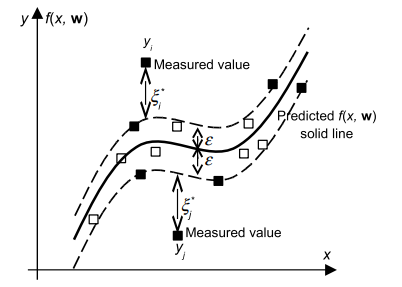
In the regression, we estimate the functional dependence of the dependent (output) variable $y \in \Re$ on an $m$-dimensional input variable $\mathbf{x}$. Thus, unlike in pattern recognition problems (where the desired outputs $y_{i}$ are discrete values e.g., Boolean) we deal with real valued functions and we model an $\Re^{m}$ to $\Re^{1}$ mapping here. Same as in the case of classification, this will be achieved by training the SVM model on a training data set first. Interestingly and importantly, a learning stage will end in the same shape of a dual Lagrangian as in classification, only difference being in a dimensionalities of the Hessian matrix and corresponding vectors which are of a double size now e.g., $\mathbf{H}$ is a $(2 n, 2 n)$ matrix. Initially developed for solving classification problems, SV techniques can be successfully applied in regression, i.e., for a functional approximation problems $[45,142]$. The general regression learning problem is set as follows – the learning machine is given $n$ training data from which it attempts to learn the input-output relationship (dependency, mapping or function) $f(\mathbf{x})$. A training data set $\mathcal{X}=[\mathbf{x}(i), y(i)] \in \Re^{m} \times \Re, i=1, \ldots, n$ consists of $n$ pairs $\left(\mathbf{x}{1}, y{1}\right),\left(\mathbf{x}{2}, y{2}\right), \ldots,\left(\mathbf{x}{n}, y{n}\right)$, where the inputs $\mathbf{x}$ are $m$-dimensional vectors $\mathbf{x} \in \Re^{m}$ and system responses $y \in \Re$, are continuous values. We introduce all the relevant and necessary concepts of SVM’s regression in a gentle way starting again with a linear regression hyperplane $f(\mathbf{x}, \mathbf{w})$ given as $$ f(\mathbf{x}, \mathbf{w})=\mathbf{w}^{T} \mathbf{x}+b $$ In the case of SVM’s regression, we measure the error of approximation instead of the margin used in classification. The most important difference in respect to classic regression is that we use a novel loss (error) functions here. This is the Vapnik’s linear loss function with e-insensitivity zone defined as $$ E(\mathbf{x}, y, f)=|y-f(\mathbf{x}, \mathbf{w})|_{e}= \begin{cases}0 & \text { if }|y-f(\mathbf{x}, \mathbf{w})| \leq \varepsilon \ |y-f(\mathbf{x}, \mathbf{w})|-\varepsilon & \text { otherwise }\end{cases} $$
or as, $$ E(\mathbf{x}, y, f)=\max (0,|y-f(\mathbf{x}, \mathbf{w})|-\varepsilon) $$ Thus, the loss is equal to zero if the difference between the predicted $f\left(\mathbf{x}{i}, \mathbf{w}\right)$ and the measured value $y{i}$ is less than $\varepsilon$. In contrast, if the difference is larger than $\varepsilon$, this difference is used as the error. Vapnik’s $\varepsilon$-insensitivity loss function (2.40) defines an $\varepsilon$ tube as shown in Fig. 2.18. If the predicted value is within the tube, the loss (error or cost) is zero. For all other predicted points outside the tube, the loss equals the magnitude of the difference between the predicted value and the radius $\varepsilon$ of the tube.
机器学习代写|监督学习代考Supervised and Unsupervised learning代写|Implementation Issues
In both the classification and the regression the learning problem boils down to solving the QP problem subject to the so-called ‘box-constraints’ and to the equality constraint in the case that a model with a bias term $b$ is used. The SV training works almost perfectly for not too large data basis. However, when the number of data points is large (say $n>2,000$ ) the QP problem becomes extremely difficult to solve with standard QP solvers and methods. For example, a classification training set of 50,000 examples amounts to a Hessian matrix $\mathbf{H}$ with $2.5 * 10^{9}$ (2.5 billion) elements. Using an 8 -byte floating-point representation we need 20,000 Megabytes $=20$ Gigabytes of memory [109]. This cannot be easily fit into memory of present standard computers, and this is the single basic disadvantage of the SVM method. There are three approaches that resolve the QP for large data sets. Vapnik in [144] proposed the chunking method that is the decomposition approach. Another decomposition approach is suggested in [109]. The sequential minimal optimization [115] algorithm is of different character and it seems to be an ‘error back propagation’ for an SVM learning. A systematic exposition of these various techniques is not given here, as all three would require a lot of space. However, the interested reader can find a description and discussion about the algorithms mentioned above in next chapter and $[84,150]$. The Vogt and Kecman’s chapter $[150]$ discusses the application of an active set algorithm in solving small to medium sized QP problems. For such data sets and when the high precision is required the active set approach in solving QP problems seems to be superior to other approaches (notably to the interior point methods and to the sequential minimal optimization (SMO) algorithm). Next chapter introduces the efficient iterative single data algorithm (ISDA) for solving huge data sets (say more than 100,000 or 500,000 or over 1 million training data pairs).
机器学习代写|监督学习代考Supervised and Unsupervised learning代写|Iterative Single Data Algorithm
One of the mainstream research fields in learning from empirical data by support vector machines (SVMs), and solving both the classification and the regression problems is an implementation of the iterative (incremental) learning schemes when the training data set is huge. The challenge of applying SVMs on huge data sets comes from the fact that the amount of computer memory required for solving the quadratic programming (QP) problem presented in the previous chapter increases drastically with the size of the training data set $n$. Depending on the memory requirement, all the solvers of SVMs can be classified into one of the three basic types as shown in Fig. 3.1 [150]. Direct methods (such as interior point methods) can efficiently obtain solution in machine precision, but they require at least $\mathcal{O}\left(n^{2}\right)$ of memory to store the Hessian matrix of the QP problem. As a result, they are often used to solve small-sized problems which require high precision. At the other end of the spectrum are the working-set (decomposition) algorithms whose memory requirements are only $\mathcal{O}\left(n+q^{2}\right)$ where $q$ is the size of the working-set (for the ISDAs developed in this book, $q$ is equal to 1). The reason for the low memory footprint is due to the fact that the solution is obtained iteratively instead of directly as in most of the QP solvers. They are the only possible algorithms for solving large-scale learning problems, but they are not suitable for obtaining high precision solutions because of the iterative nature of the algorithm. The relative size of the learning problem depends on the computer being used. As a result, a learning problem will be regarded as a “large” or “huge” problem in this book if the Hessian matrix of its unbounded SVs $\left(\mathbf{H}{S{f}} S_{f}\right.$ where $S_{f}$ denotes the set of free SVs) cannot be stored in the computer memory. Between the two ends of the spectrum are the active-set algorithms $[150]$ and their memory requirements are $\mathcal{O}\left(N_{F S V}^{2}\right)$, i.e. they depend on the number of unbounded support vectors of the problem. The main focus of this book is to develop efficient algorithms that can solve large-scale QP problems for SVMs in practice. Although many applications in engineering also require the solving of large-scale QP problems (and there are many solvers available), the QP problems induced by SVMs are different from these applications. In the case of SVMs, the Hessian matrix of (2.38a) is extremely dense, whereas in most of the engineering applications, the optimization problems have relatively sparse Hessian matrices. This is why many of the existing QP solvers are not suitable for SVMs and new approaches need to be invented and developed. Among several candidates that avoid the use of standard QP solvers, the two learning approaches which recently have drawn the attention are the Iterative Single Data Algorithm (ISDA), and the Sequential Minimal Optimization (SMO) $[69,78,115,148]$.
机器学习代写|监督学习代考Supervised and Unsupervised learning代写|Regression by Support Vector Machines
statistics-lab™ 为您的留学生涯保驾护航 在代写监督学习Supervised and Unsupervised learning方面已经树立了自己的口碑, 保证靠谱, 高质且原创的统计Statistics代写服务。我们的专家在代写监督学习Supervised and Unsupervised learning代写方面经验极为丰富,各种代写监督学习Supervised and Unsupervised learning相关的作业也就用不着说。
我们提供的监督学习Supervised and Unsupervised learning及其相关学科的代写,服务范围广, 其中包括但不限于:
Statistical Inference 统计推断
Statistical Computing 统计计算
Advanced Probability Theory 高等概率论
Advanced Mathematical Statistics 高等数理统计学
(Generalized) Linear Models 广义线性模型
Statistical Machine Learning 统计机器学习
Longitudinal Data Analysis 纵向数据分析
Foundations of Data Science 数据科学基础
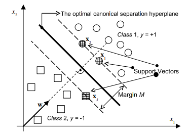
机器学习代写|监督学习代考Supervised and Unsupervised learning代写|Linear Maximal Margin Classifier for Linearly Separable Data
机器学习代写|监督学习代考Supervised and Unsupervised learning代写|Linear Maximal Margin Classifier for Linearly Separable Data
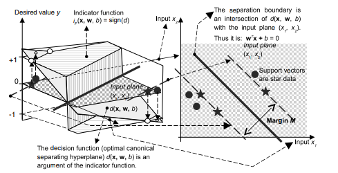
Consider the problem of binary classification or dichotomization. Training data are given as $$ \left(\mathbf{x}{1}, y\right),\left(\mathbf{x}{2}, y\right), \ldots,\left(\mathbf{x}{n}, y{n}\right), \mathbf{x} \in \Re^{m}, \quad y \in{+1,-1} $$ For reasons of visualization only, we will consider the case of a two-dimensional input space, i.e., $\left(\mathbf{x} \in \Re^{2}\right)$. Data are linearly separable and there are many
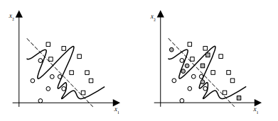
different hyperplanes that can perform separation (Fig. 2.5). (Actually, for $\mathbf{x} \in \Re^{2}$, the separation is performed by ‘planes’ $w_{1} x_{1}+w_{2} x_{2}+b=d$. In other words, the decision boundary, i.e., the separation line in input space is defined by the equation $w_{1} x_{1}+w_{2} x_{2}+b=0$.). How to find ‘the best’ one? The difficult part is that all we have at our disposal are sparse training data. Thus, we want to find the optimal separating function without knowing the underlying probability distribution $P(\mathbf{x}, y)$. There are many functions that can solve given pattern recognition (or functional approximation) tasks. In such a problem setting, the SLT (developed in the early 1960 s by Vapnik and Chervonenkis [145]) shows that it is crucial to restrict the class of functions implemented by a learning machine to one with a complexity that is suitable for the amount of available training data.
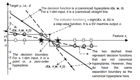
In the case of a classification of linearly separable data, this idea is transformed into the following approach – among all the hyperplanes that minimize the training error (i.e., empirical risk) find the one with the largest margin. This is an intuitively acceptable approach. Just by looking at Fig $2.5$ we will find that the dashed separation line shown in the right graph seems to promise probably good classification while facing previously unseen data (meaning, in the generalization, i.e. test, phase). Or, at least, it seems to probably be better in generalization than the dashed decision boundary having smaller margin shown in the left graph. This can also be expressed as that a classifier with smaller margin will have higher expected risk. By using given training examples, during the learning stage, our machine finds parameters $\mathbf{w}=\left[\begin{array}{llll}w_{1} & w_{2} & \ldots & w_{m}\end{array}\right]^{T}$ and $b$ of a discriminant or decision function $d(\mathbf{x}, \mathbf{w}, b)$ given as
$$ d(\mathbf{x}, \mathbf{w}, b)=\mathbf{w}^{T} \mathbf{x}+b=\sum_{i=1}^{m} w_{i} x_{i}+b $$ where $\mathbf{x}, \mathbf{w} \in \Re^{m}$, and the scalar $b$ is called a bias.(Note that the dashed separation lines in Fig. $2.5$ represent the line that follows from $d(\mathbf{x}, \mathbf{w}, b)=0)$. After the successful training stage, by using the weights obtained, the learning machine, given previously unseen pattern $\mathbf{x}{p}$, produces output $o$ according to an indicator function given as $$ i{F}=o=\operatorname{sign}\left(d\left(\mathbf{x}_{p}, \mathbf{w}, b\right)\right) . $$
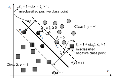
机器学习代写|监督学习代考Supervised and Unsupervised learning代写|Linear Soft Margin Classifier for Overlapping Classe
The learning procedure presented above is valid for linearly separable data, meaning for training data sets without overlapping. Such problems are rare in practice. At the same time, there are many instances when linear separating hyperplanes can be good solutions even when data are overlapped (e.g., normally distributed classes having the same covariance matrices have a linear separation boundary). However, quadratic programming solutions as given above cannot be used in the case of overlapping because the constraints $y_{i}\left[\mathbf{w}^{T} \mathbf{x}{i}+b\right] \geq 1, i=1, n$ given by (2.10b) cannot be satisfied. In the case of an overlapping (see Fig. 2.10), the overlapped data points cannot be correctly classified and for any misclassified training data point $\mathbf{x}{i}$, the corresponding $\alpha_{i}$ will tend to infinity. This particular data point (by increasing the corresponding $\alpha_{i}$ value) attempts to exert a stronger influence on the decision boundary in order to be classified correctly. When the $\alpha_{i}$ value reaches the maximal bound, it can no longer increase its effect, and the corresponding point will stay misclassified. In such a situation, the algorithm introduced above chooses all training data points as support vectors. To find a classifier with a maximal margin, the algorithm presented in the Sect. 2.2.1, must be changed allowing some data to be unclassified. Better to say, we must leave some data on the ‘wrong’ side of a decision boundary. In practice, we allow a soft margin and all data inside this margin (whether on the correct side of the separating line or on the wrong one) are neglected. The width of a soft margin can be controlled by a corresponding penalty parameter $C$ (introduced below) that determines the trade-off between the training error and VC dimension of the model. The question now is how to measure the degree of misclassification and how to incorporate such a measure into the hard margin learning algorithm given by (2.10). The simplest method would be to form the following learning problem $$ \min \frac{1}{2} \mathbf{w}^{T} \mathbf{w}+C \text { (number of misclassified data) } $$ where $C$ is a penalty parameter, trading off the margin size (defined by $|\mathbf{w}|$, i.e., by $\mathbf{w}^{T} \mathbf{w}$ ) for the number of misclassified data points. Large $C$ leads to small number of misclassifications, bigger $\mathbf{w}^{T} \mathbf{w}$ and consequently to the smaller margin and vice versa. Obviously taking $C=\infty$ requires that the number of misclassified data is zero and, in the case of an overlapping this is not possible. Hence, the problem may be feasible only for some value $C<\infty$.
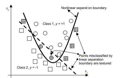
机器学习代写|监督学习代考Supervised and Unsupervised learning代写|The Nonlinear SVMs Classifier
The linear classifiers presented in two previous sections are very limited. Mostly, classes are not only overlapped but the genuine separation functions are nonlinear hypersurfaces. A nice and strong characteristic of the approach presented above is that it can be easily (and in a relatively straightforward manner) extended to create nonlinear decision boundaries. The motivation for such an extension is that an SV machine that can create a nonlinear decision hypersurface will be able to classify nonlinearly separable data. This will be achieved by considering a linear classifier in the so-called feature space that will be introduced shortly. A very simple example of a need for designing nonlinear models is given in Fig. $2.11$ where the true separation boundary is quadratic. It is obvious that no errorless linear separating hyperplane can be found now. The best linear separation function shown as a dashed straight line would make six misclassifications (textured data points; 4 in the negative class and 2 in the positive one). Yet, if we use the nonlinear separation boundary we are able to separate two classes without any error. Generally, for $n$-dimensional input patterns, instead of a nonlinear curve, an SV machine will create a nonlinear separating hypersurface.
机器学习代写|监督学习代考Supervised and Unsupervised learning代写|Linear Maximal Margin Classifier for Linearly Separable Data
statistics-lab™ 为您的留学生涯保驾护航 在代写监督学习Supervised and Unsupervised learning方面已经树立了自己的口碑, 保证靠谱, 高质且原创的统计Statistics代写服务。我们的专家在代写监督学习Supervised and Unsupervised learning代写方面经验极为丰富,各种代写监督学习Supervised and Unsupervised learning相关的作业也就用不着说。
我们提供的监督学习Supervised and Unsupervised learning及其相关学科的代写,服务范围广, 其中包括但不限于:
Statistical Inference 统计推断
Statistical Computing 统计计算
Advanced Probability Theory 高等概率论
Advanced Mathematical Statistics 高等数理统计学
(Generalized) Linear Models 广义线性模型
Statistical Machine Learning 统计机器学习
Longitudinal Data Analysis 纵向数据分析
Foundations of Data Science 数据科学基础
机器学习代写|监督学习代考Supervised and Unsupervised learning代写|Support Vector Machines
机器学习代写|监督学习代考Supervised and Unsupervised learning代写|Regression – An Introduction
This is an introductory chapter on the supervised (machine) learning from empirical data (i.e., examples, samples, measurements, records, patterns or observations) by applying support support vector machines (SVMs) a.k.a. kernel machines $^{1}$. The parts on the semi-supervised and unsupervised learning are given later and being entirely different tasks they use entirely different math and approaches. This will be shown shortly. Thus, the book introduces the problems gradually in an order of loosing the information about the desired output label. After the supervised algorithms, the semi-supervised ones will be presented followed by the unsupervised learning methods in Chap. 6 . The basic aim of this chapter is to give, as far as possible, a condensed (but systematic) presentation of a novel learning paradigm embodied in SVMs. Our focus will be on the constructive part of the SVMs’ learning algorithms for both the classification (pattern recognition) and regression (function approximation) problems. Consequently, we will not go into all the subtleties and details of the statistical learning theory (SLT) and structural risk minimization (SRM) which are theoretical foundations for the learning algorithms presented below. The approach here seems more appropriate for the application oriented readers. The theoretically minded and interested reader may find an extensive presentation of both the SLT and SRM in $[146,144,143,32,42,81,123]$. Instead of diving into a theory, a quadratic programming based learning, leading to parsimonious SVMs, will be presented in a gentle way – starting with linear separable problems, through the classification tasks having overlapped classes but still a linear separation boundary, beyond the linearity assumptions to the nonlinear separation boundary, and finally to the linear and nonlinear regression problems. Here, the adjective ‘parsimonious’ denotes a SVM with a small number of support vectors (‘hidden layer neurons’). The scarcity of the model results from a sophisticated, QP based, learning that matches the
model capacity to data complexity ensuring a good generalization, i.e., a good performance of SVM on the future, previously, during the training unseen, data.
Same as the neural networks (or similarly to them), SVMs possess the wellknown ability of being universal approximators of any multivariate function to any desired degree of accuracy. Consequently, they are of particular interest for modeling the unknown, or partially known, highly nonlinear, complex systems, plants or processes. Also, at the very beginning, and just to be sure what the whole chapter is about, we should state clearly when there is no need for an application of SVMs’ model-building techniques. In short, whenever there exists an analytical closed-form model (or it is possible to devise one) there is no need to resort to learning from empirical data by SVMs (or by any other type of a learning machine)
机器学习代写|监督学习代考Supervised and Unsupervised learning代写|Basics of Learning from Data
SVMs have been developed in the reverse order to the development of neural networks (NNs). SVMs evolved from the sound theory to the implementation and experiments, while the NNs followed more heuristic path, from applications and extensive experimentation to the theory. It is interesting to note that the very strong theoretical background of SVMs did not make them widely appreciated at the beginning. The publication of the first papers by Vapnik and Chervonenkis [145] went largely unnoticed till 1992 . This was due to a widespread belief in the statistical and/or machine learning community that, despite being theoretically appealing, SVMs are neither suitable nor relevant for practical applications. They were taken seriously only when excellent results on practical learning benchmarks were achieved (in numeral recognition, computer vision and text categorization). Today, SVMs show better results than (or comparable outcomes to) NNs and other statistical models, on the most popular benchmark problems.
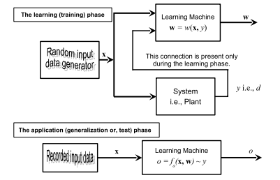
The learning problem setting for SVMs is as follows: there is some unknown and nonlinear dependency (mapping, function) $y=f(\mathbf{x})$ between some high-dimensional input vector $\mathbf{x}$ and the scalar output $y$ (or the vector output $\mathbf{y}$ as in the case of multiclass SVMs). There is no information about the underlying joint probability functions here. Thus, one must perform a distribution-free learning. The only information available is a training data set $\left{\mathcal{X}=[\mathbf{x}(i), y(i)] \in \mathfrak{R}^{m} \times \mathfrak{R}, i=1, \ldots, n\right}$, where $n$ stands for the number of the training data pairs and is therefore equal to the size of the training data set $\mathcal{X}$. Often, $y_{i}$ is denoted as $d_{i}$ (i.e., $t_{i}$ ), where $d(t)$ stands for a desired (target) value. Hence, SVMs belong to the supervised learning techniques. Note that this problem is similar to the classic statistical inference. However, there are several very important differences between the approaches and assumptions in training SVMs and the ones in classic statistics and/or NNs
modeling. Classic statistical inference is based on the following three fundamental assumptions:
Data can be modeled by a set of linear in parameter functions; this is a foundation of a parametric paradigm in learning from experimental data.
In the most of real-life problems, a stochastic component of data is the normal probability distribution law, that is, the underlying joint probability distribution is a Gaussian distribution.
Because of the second assumption, the induction paradigm for parameter estimation is the maximum likelihood method, which is reduced to the minimization of the sum-of-errors-squares cost function in most engineering applications.
All three assumptions on which the classic statistical paradigm relied turned out to be inappropriate for many contemporary real-life problems [143] because of the following facts:
Modern problems are high-dimensional, and if the underlying mapping is not very smooth the linear paradigm needs an exponentially increasing number of terms with an increasing dimensionality of the input space (an increasing number of independent variables). This is known as ‘the curse of dimensionality’.
The underlying real-life data generation laws may typically be very far from the normal distribution and a model-builder must consider this difference in order to construct an effective learning algorithm.
From the first two points it follows that the maximum likelihood estimator (and consequently the sum-of-error-squares cost function) should be replaced by a new induction paradigm that is uniformly better, in order to model non-Gaussian distributions.
机器学习代写|监督学习代考Supervised and Unsupervised learning代写|Support Vector Machines in Classification
Below, we focus on the algorithm for implementing the SRM induction principle on the given set of functions. It implements the strategy mentioned previously – it keeps the training error fixed and minimizes the confidence interval. We first consider a ‘simple’ example of linear decision rules (i.e., the separating functions will be hyperplanes) for binary classification (dichotomization) of linearly separable data. In such a problem, we are able to perfectly classify data pairs, meaning that an empirical risk can be set to zero. It is the easiest classification problem and yet an excellent introduction of all relevant and important ideas underlying the SLT, SRM and SVM.
Our presentation will gradually increase in complexity. It will begin with a Linear Maximal Margin Classifier for Linearly Separable Data where there is no sample overlapping. Afterwards, we will allow some degree of overlapping of training data pairs. However, we will still try to separate classes by using linear hyperplanes. This will lead to the Linear Soft Margin Classifier for Overlapping Classes. In problems when linear decision hyperplanes are no longer feasible, the mapping of an input space into the so-called feature space (that ‘corresponds’ to the HL in NN models) will take place resulting in the Nonlinear Classifier. Finally, in the subsection on Regression by SV Machines we introduce same approaches and techniques for solving regression (i.e., function approximation) problems.
机器学习代写|监督学习代考Supervised and Unsupervised learning代写|Support Vector Machines
statistics-lab™ 为您的留学生涯保驾护航 在代写监督学习Supervised and Unsupervised learning方面已经树立了自己的口碑, 保证靠谱, 高质且原创的统计Statistics代写服务。我们的专家在代写监督学习Supervised and Unsupervised learning代写方面经验极为丰富,各种代写监督学习Supervised and Unsupervised learning相关的作业也就用不着说。
我们提供的监督学习Supervised and Unsupervised learning及其相关学科的代写,服务范围广, 其中包括但不限于:
Statistical Inference 统计推断
Statistical Computing 统计计算
Advanced Probability Theory 高等概率论
Advanced Mathematical Statistics 高等数理统计学
(Generalized) Linear Models 广义线性模型
Statistical Machine Learning 统计机器学习
Longitudinal Data Analysis 纵向数据分析
Foundations of Data Science 数据科学基础
机器学习代写|监督学习代考Supervised and Unsupervised learning代写|Feature Reduction with Support Vector Machines
机器学习代写|监督学习代考Supervised and Unsupervised learning代写|Feature Reduction with Support Vector Machines
Recently, more and more instances have occurred in which the learning problems are characterized by the presence of a small number of the highdimensional training data points, i.e. $n$ is small and $m$ is large. This often occurs in the bioinformatics area where obtaining training data is an expensive and time-consuming process. As mentioned previously, recent advances in the DNA microarray technology allow biologists to measure several thousands of genes’ expressions in a single experiment. However, there are three basic reasons why it is not possible to collect many DNA microarrays and why we have to work with sparse data sets. First, for a given type of cancer it is not simple to have thousands of patients in a given time frame. Second, for many cancer studies, each tissue sample used in an experiment needs to be obtained by surgically removing cancerous tissues and this is an expensive and time consuming procedure. Finally, obtaining the DNA microarrays is still expensive technology. As a result, it is not possible to have a relatively large quantity of training examples available. Generally, most of the microarray studies have a few dozen of samples, but the dimensionality of the feature spaces (i.e. space of input vector $\mathbf{x}$ ) can be as high as several thousand. In such cases, it is difficult to produce a classifier that can generalize well on the unseen data, because the amount of training data available is insufficient to cover the high dimensional feature space. It is like trying to identify objects in a big dark room with only a few lights turned on. The fact that $n$ is much smaller than $m$ makes this problem one of the most challenging tasks in the areas of machine learning, statistics and bioinformatics.
The problem of having high-dimensional feature space led to the idea of selecting the most relevant set of genes or features first, and only then the classifier is constructed from these selected and “important”‘ features by the learning algorithms. More precisely, the classifier is constructed over a reduced space (and, in the comparative example above, this corresponds to an object identification in a smaller room with the same number of lights). As a result such a classifier is more likely to generalize well on the unseen data. In the book, a feature reduction technique based on SVMs (dubbed Recursive Feature Elimination with Support Vector Machines (RFE-SVMs)) developed in [61], is implemented and improved. In particular, the focus is on gene selection for cancer diagnosis using RFE-SVMs. RFE-SVM is included in the book because it is the most natural way to harvest the discriminative power of SVMs for microarray analysis. At the same time, it is also a natural extension of the work on solving SVMs efficiently. The original contributions presented in the book in this particular area are as follows:
机器学习代写|监督学习代考Supervised and Unsupervised learning代写|Graph-Based Semi-supervised Learning Algorithms
As mentioned previously, semi-supervised learning (SSL) is the latest development in the field of machine learning. It is driven by the fact that in many real-world problems the cost of labeling data can be quite high and there is an abundance of unlabeled data. The original goal of this book was to develop large-scale solvers for SVMs and apply SVMs to real-world problems only. However, it was found that some of the techniques developed in SVMs can be extended naturally to the graph-based semi-supervised learning, because the optimization problems associated with both learning techniques are identical (more details shortly).
In the book, two very popular graph-based semi-supervised learning algorithms, namely, the Gaussian random fields model (GRFM) introduced in $[160]$ and $[159]$, and the consistency method (CM) for semi-supervised learning proposed in [155] were improved. The original contributions to the field of SSL presented in this book are as follows:
An introduction of the novel normalization step into both CM and GRFM. This additional step improves the performance of both algorithms significantly in the cases where labeled data are unbalanced. The labeled data are regarded as unbalanced when each class has a different number of labeled data in the training set. This contribution is presented in Sect. $5.3$ and 5.4.
The world first large-scale graph-based semi-supervised learning software SemiL is developed as part of this book. The software is based on a Conjugate Gradient (CG) method which can take box-constraints into account and it is used as a backbone for all the simulation results in Chap. $5 .$ Furthermore, SemiL has become a very popular tool in this area at the time of writing this book, with approximately 100 downloads per month. The details of this contribution are given in Sect. $5.6$.
机器学习代写|监督学习代考Supervised and Unsupervised learning代写|Unsupervised Learning Based on Principle
SVMs as the latest supervised learning technique from the statistical learning theory as well as any other supervised learning method require labeled data in
order to train the learning machine. As already mentioned, in many real world problems the cost of labeling data can be quite high. This presented motivation for most recent development of the semi-supervised learning where only small amount of data is assumed to be labeled. However, there exist classification problems where accurate labeling of the data is sometime even impossible. One such application is classification of remotely sensed multispectral and hyperspectral images $[46,47]$. Recall that typical family RGB color image (photo) contains three spectral bands. In other words we can say that family photo is a three-spectral image. A typical hyperspectral image would contain more than one hundred spectral bands. As remote sensing and its applications receive lots of interests recently, many algorithms in remotely sensed image analysis have been proposed [152]. While they have achieved a certain level of success, most of them are supervised methods, i.e., the information of the objects to be detected and classified is assumed to be known a priori. If such information is unknown, the task will be much more challenging. Since the area covered by a single pixel is very large, the reflectance of a pixel can be considered as the mixture of all the materials resident in the area covered by the pixel. Therefore, we have to deal with mixed pixels instead of pure pixels as in conventional digital image processing. Linear spectral unmixing analysis is a popular approach used to uncover material distribution in an image scene $[127,2,125,3]$. Formally, the problem is stated as: $$ \mathbf{r}=\mathbf{M} \alpha+\mathbf{n} $$ where $\mathbf{r}$ is a reflectance column pixel vector with dimension $L$ in a hyperspectral image with $L$ spectral bands. An element $r_{i}$ in the $\mathbf{r}$ is the reflectance collected in the $i^{\text {th }}$ wavelength band. $\mathbf{M}$ denotes a matrix containing $p$ independent material spectral signatures (referred to as endmembers in linear mixture model), i.e., $\mathbf{M}=\left[\mathbf{m}{1}, \mathbf{m}{2}, \ldots, \mathbf{m}{p}\right], \boldsymbol{\alpha}$ represents the unknown abundance column vector of size $p \times 1$ associated with $\mathbf{M}$, which is to be estimated and $\mathbf{n}$ is the noise term. The $i^{t h}$ item $\alpha{i}$ in $\boldsymbol{\alpha}$ represents the abundance fraction of $\mathbf{m}_{i}$ in pixel $\mathbf{r}$. When $\mathbf{M}$ is known, the estimation of $\boldsymbol{\alpha}$ can be accomplished by least squares approach. In practice, it may be difficult to have prior information about the image scene and endmember signatures. Moreover, in-field spectral signatures may be different from those in spectral libraries due to atmospheric and environmental effects. So an unsupervised classification approach is preferred. However, when $\mathbf{M}$ is also unknown, i.e., in unsupervised analysis, the task is much more challenging since both $\mathbf{M}$ and $\boldsymbol{\alpha}$ need to be estimated [47]. Under stated conditions the problem represented by linear mixture model (1.3) can be interpreted as a linear instantaneous blind source separation (BSS) problem [76] mathematically described as: $$ \mathbf{x}=\mathbf{A s}+\mathbf{n} $$ where x represents data vector, $\mathbf{A}$ is unknown mixing matrix, $\mathbf{s}$ is vector of source signals or classes to be found by an unsupervised method and $\mathbf{n}$ is again additive noise term.
机器学习代写|监督学习代考Supervised and Unsupervised learning代写|Feature Reduction with Support Vector Machines
机器学习代写|监督学习代考Supervised and Unsupervised learning代写|Feature Reduction with Support Vector Machines
最近,出现了越来越多的例子,其中学习问题的特点是存在少量的高维训练数据点,即n很小而且米很大。这通常发生在生物信息学领域,其中获取训练数据是一个昂贵且耗时的过程。如前所述,DNA 微阵列技术的最新进展允许生物学家在一次实验中测量数千个基因的表达。然而,为什么不可能收集许多 DNA 微阵列以及为什么我们必须使用稀疏数据集有三个基本原因。首先,对于给定类型的癌症,在给定的时间范围内拥有数千名患者并不容易。其次,对于许多癌症研究,实验中使用的每个组织样本都需要通过手术切除癌组织获得,这是一个昂贵且耗时的过程。最后,获得 DNA 微阵列仍然是一项昂贵的技术。因此,不可能有相对大量的训练示例可用。通常,大多数微阵列研究都有几十个样本,但特征空间的维数(即输入向量的空间)X) 可高达数千。在这种情况下,很难产生一个可以很好地概括看不见的数据的分类器,因为可用的训练数据量不足以覆盖高维特征空间。这就像在一个只有几盏灯打开的大黑暗房间里试图识别物体。事实是n远小于米使这个问题成为机器学习、统计学和生物信息学领域最具挑战性的任务之一。
statistics-lab™ 为您的留学生涯保驾护航 在代写监督学习Supervised and Unsupervised learning方面已经树立了自己的口碑, 保证靠谱, 高质且原创的统计Statistics代写服务。我们的专家在代写监督学习Supervised and Unsupervised learning代写方面经验极为丰富,各种代写监督学习Supervised and Unsupervised learning相关的作业也就用不着说。
我们提供的监督学习Supervised and Unsupervised learning及其相关学科的代写,服务范围广, 其中包括但不限于:
Statistical Inference 统计推断
Statistical Computing 统计计算
Advanced Probability Theory 高等概率论
Advanced Mathematical Statistics 高等数理统计学
(Generalized) Linear Models 广义线性模型
Statistical Machine Learning 统计机器学习
Longitudinal Data Analysis 纵向数据分析
Foundations of Data Science 数据科学基础
机器学习代写|监督学习代考Supervised and Unsupervised learning代写|An Overview of Machine Learning
机器学习代写|监督学习代考Supervised and Unsupervised learning代写|An Overview of Machine Learning
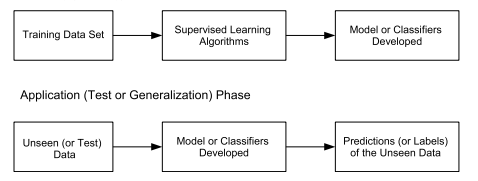
The amount of data produced by sensors has increased explosively as a result of the advances in sensor technologies that allow engineers and scientists to quantify many processes in fine details. Because of the sheer amount and complexity of the information available, engineers and scientists now rely heavily on computers to process and analyze data. This is why machine learning has become an emerging topic of research that has been employed by an increasing number of disciplines to automate complex decision-making and problem-solving tasks. This is because the goal of machine learning is to extract knowledge from experimental data and use computers for complex decision-making, i.e. decision rules are extracted automatically from data by utilizing the speed and the robustness of the machines. As one example, the DNA microarray technology allows biologists and medical experts to measure the expressiveness of thousands of genes of a tissue sample in a single experiment. They can then identify cancerous genes in a cancer study. However, the information that is generated from the DNA microarray experiments and many other measuring devices cannot be processed or analyzed manually because of its large size and high complexity. In the case of the cancer study, the machine learning algorithm has become a valuable tool to identify the cancerous genes from the thousands of possible genes. Machine-learning techniques can be divided into three major groups based on the types of problems they can solve, namely, the supervised, semi-supervised and unsupervised learning. The supervised learning algorithm attempts to learn the input-output relationship (dependency or function) $f(x)$ by using a training data set $\left{\mathcal{X}=\left[\mathbf{x}{i}, y{i}\right], i=1, \ldots, n\right}$ consisting of $n$ pairs $\left(\mathbf{x}{1}, y{1}\right),\left(\mathbf{x}{2}, y{2}\right), \ldots\left(\mathbf{x}{n}, y{n}\right)$, where the inputs $\mathbf{x}$ are $m$-dimensional vectors $\mathbf{x} \in \Re^{m}$ and the labels (or system responses) $y$ are discrete (e.g., Boolean) for classification problems and continuous values $(y \in \Re)$ for regression tasks. Support Vector Machines (SVMs) and Artificial Neural Network (ANN) are two of the most popular techniques in this area.
There are two types of supervised learning problems, namely, classification (pattern recognition) and the regression (function approximation) ones. In the classification problem, the training data set consists of examples from different classes. The simplest classification problem is a binary one that consists of training examples from two different classes ( $+1$ or $-1$ class). The outputs $y_{i} \in{1,-1}$ represent the class belonging (i.e. labels) of the corresponding input vectors $\mathbf{x}{i}$ in the classification. The input vectors $\mathbf{x}{i}$ consist of measurements or features that are used for differentiating examples of different classes. The learning task in classification problems is to construct classifiers that can classify previously unseen examples $\mathbf{x}_{j}$. In other words, machines have to learn from the training examples first, and then they should make complex decisions based on what they have learned. In the case of multi-class problems, several binary classifiers are built and used for predicting the labels of the unseen data, i.e. an $N$-class problem is generally broken down into $N$ binary classification problems. The classification problems can be found in many different areas, including, object recognition, handwritten recognition, text classification, disease analysis and DNA microarray studies. The term “supervised” comes from the fact that the labels of the training data act as teachers who educate the learning algorithms.
机器学习代写|监督学习代考Supervised and Unsupervised learning代写|Challenges in Machine Learning
Like most areas in science and engineering, machine learning requires developments in both theoretical and practical (engineering) aspects. An activity on the theoretical side is concentrated on inventing new theories as the foundations for constructing novel learning algorithms. On the other hand, by extending existing theories and inventing new techniques, researchers who work in the engineering aspects of the field try to improve the existing learning algorithms and apply them to the novel and challenging real-world problems. This book is focused on the practical aspects of SVMs, graph-based semisupervised learning algorithms and two basic unsupervised learning methods. More specifically, it aims at making these learning techniques more practical for the implementation to the real-world tasks. As a result, the primary goal of this book is aimed at developing novel algorithms and software that can solve large-scale SVMs, graph-based semi-supervised and unsupervised learning problems. Once an efficient software implementation has been obtained, the goal will be to apply these learning techniques to real-world problems and to improve their performance. Next four sections outline the original contributions of the book in solving the mentioned tasks.
机器学习代写|监督学习代考Supervised and Unsupervised learning代写|Solving Large-Scale SVMs
As mentioned previously, machine learning techniques allow engineers and scientists to use the power of computers to process and analyze large amounts of information. However, the amount of information generated by sensors can easily go beyond the processing power of the latest computers available. As a result, one of the mainstream research fields in learning from empirical data is to design learning algorithms that can be used in solving large-scale problems efficiently. The book is primarily aimed at developing efficient algorithms for implementing SVMs. SVMs are the latest supervised learning techniques from statistical learning theory and they have been shown to deliver state-of-the-art performance in many real-world applications [153]. The challenge of applying SVMs on huge data sets comes from the fact that the amount of computer memory required for solving the quadratic programming (QP) problem associated with SVMs increases drastically with the size of the training data set $n$ (more details can be found in Chap. 3). As a result, the book aims at providing a better solution for solving large-scale SVMs using iterative algorithms. The novel contributions presented in this book are as follows:
The development of Iterative Single Data Algorithm (ISDA) with the explicit bias term $b$. Such a version of ISDA has been shown to perform better (faster) than the standard SVMs learning algorithms achieving at the same time the same accuracy. These contributions are presented in Sect. $3.3$ and 3.4.
An efficient software implementation of the ISDA is developed. The ISDA software has been shown to be significantly faster than the well-known SVMs learning software LIBSVM [27]. These contributions are presented in Sect. 3.5.
机器学习代写|监督学习代考Supervised and Unsupervised learning代写|An Overview of Machine Learning
有两种类型的监督学习问题,即分类(模式识别)和回归(函数逼近)问题。在分类问题中,训练数据集由来自不同类别的示例组成。最简单的分类问题是由来自两个不同类别的训练样本组成的二元分类问题(+1或者−1班级)。输出是一世∈1,−1表示对应输入向量的所属类别(即标签)X一世在分类中。输入向量X一世由用于区分不同类别示例的测量值或特征组成。分类问题中的学习任务是构造分类器,可以对以前未见过的示例进行分类Xj. 换句话说,机器必须首先从训练示例中学习,然后它们应该根据所学内容做出复杂的决策。在多类问题的情况下,构建了几个二元分类器并用于预测未见数据的标签,即ñ- 类问题通常分解为ñ二元分类问题。分类问题可以在许多不同的领域中找到,包括对象识别、手写识别、文本分类、疾病分析和 DNA 微阵列研究。“监督”一词源于训练数据的标签充当教育学习算法的教师这一事实。
机器学习代写|监督学习代考Supervised and Unsupervised learning代写|Challenges in Machine Learning