数学代写|组合学代写Combinatorics代考|NWI-IBC016
如果你也在 怎样代写组合学Combinatorics 这个学科遇到相关的难题,请随时右上角联系我们的24/7代写客服。组合学Combinatorics和离散数学,在这一代人中蓬勃发展。在理论方面,各种各样的工具、概念和见解已经发展起来,使我们能够解决以前难以解决的问题,制定新的问题,并将以前不相关的主题联系起来。
组合学Combinatorics在应用方面,从物理学家到生物学家的科学家都发现组合学在他们的研究中至关重要。在所有这一切中,计算机科学和数学之间的相互作用作为理论发展和组合学应用的主要推动力而脱颖而出。本文介绍了这种相互作用的数学基础及其一些结果。
组合学Combinatorics代写,免费提交作业要求, 满意后付款,成绩80\%以下全额退款,安全省心无顾虑。专业硕 博写手团队,所有订单可靠准时,保证 100% 原创。 最高质量的组合学Combinatorics作业代写,服务覆盖北美、欧洲、澳洲等 国家。 在代写价格方面,考虑到同学们的经济条件,在保障代写质量的前提下,我们为客户提供最合理的价格。 由于作业种类很多,同时其中的大部分作业在字数上都没有具体要求,因此组合学Combinatorics作业代写的价格不固定。通常在专家查看完作业要求之后会给出报价。作业难度和截止日期对价格也有很大的影响。
statistics-lab™ 为您的留学生涯保驾护航 在代写组合学Combinatorics方面已经树立了自己的口碑, 保证靠谱, 高质且原创的统计Statistics代写服务。我们的专家在代写组合学Combinatorics代写方面经验极为丰富,各种代写组合学Combinatorics相关的作业也就用不着说。
数学代写|组合学代写Combinatorics代考|Generating Function of Permutations by Inversions
In Section 1.1, we looked at descents of permutations. That is, we studied instances in which an entry in a permutation was larger than the entry directly following it. A more “global” permutation statistic is that of inversions. This statistic will look for instances in which an entry of a permutation is smaller than some entry following it (not necessarily directly).
DEFINITION 2.1 Let $p=p_1 p_2 \cdots p_n$ be a permutation. We say that $\left(p_i, p_j\right)$ is an inversion of $p$ if $ip_j$.
Example 2.2
Permutation 31524 has four inversions, namely $(3,1),(3,2),(5,2)$, and $(5,4)$.
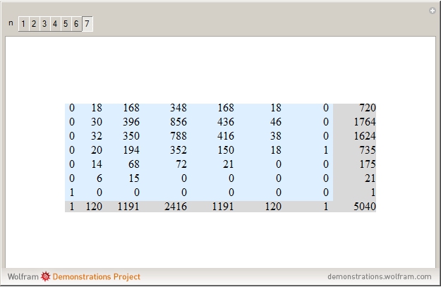
This line of research started as early as 1901 [254]. In this section, we survey some of the most interesting results in this area. The number of inversions of $p$ will be denoted by $i(p)$, though some authors prefer $i n v(p)$. It is clear that $0 \leq i(p) \leq\left(\begin{array}{c}n \ 2\end{array}\right)$ for all $n$-permutations, and that the two extreme values are attained by permutations $12 \cdots n$ and $n(n-1) \cdots 1$, respectively. It is relatively easy to find the generating function enumerating all permutations of length $n$ with respect to their number of inversions.
THEOREM 2.3
For all positive integers $n \geq 2$,
$$
\sum_{p \in S_n} z^{i(p)}=I_n(z)=(1+z)\left(1+z+z^2\right) \cdots\left(1+z+z^2+\cdots+z^{n-1}\right) .
$$
PROOF We prove the statement by induction on $n$. In fact, we prove that each of the $n$ ! expansion terms of the product $I_n(z)$ corresponds to exactly one permutation in $S_n$. Moreover, the expansion term $z^{a_1} z^{a_2} \cdots z^{a_{n-1}}$ will correspond to the unique permutation in which, for each $i \in[n]$, the entry $i+1$ precedes exactly $a_i$ entries that are smaller than itself.
If $n=2$, then there are two permutations to count, $p=12$ has no inversions, and $p^{\prime}=21$ has one inversion. So $\sum_{p \in S_2} z^{i(p)}=1+z$ as claimed. Furthermore, $p=12$ is represented by the expansion term 1 , and $p^{\prime}=21$ is represented by the expansion term $z$.
数学代写|组合学代写Combinatorics代考|Explicit Definition of Determinants
There are several undergraduate mathematics courses and textbooks that only give a recursive definition of the determinant of a square matrix. That is, $\operatorname{det}\left(\begin{array}{ll}a & b \ c & d\end{array}\right)$ is defined to be equal to $a d-b c$, and then the determinant of the $n \times n$ matrix $A=\left(a_{i j}\right)$ is defined to be
$$
\operatorname{det} A=\sum_{j=1}^n(-1)^{j-1} a_{1 j} A_{1 j}
$$
where $A_{1 j}$ is the $(n-1) \times(n-1)$ matrix obtained from $A$ by removing the first row and the $j$ th column.
If that is the only definition of determinants the reader has seen, he may find the following result interesting.
THEOREM 2.21
Let $A=\left(a_{i j}\right)$ be an $n \times n$ matrix. Then we have
$$
\operatorname{det} A=\sum_{p \in S_n}(-1)^{i(p)} a_{1 p_1} a_{2 p_2} \cdots a_{n p_n} .
$$
That is, $\operatorname{det} A$ is obtained by taking all $n$ ! possible $n$-tuples of entries so that there is exactly one of the $n$ entries in each row and each column, multiplying the elements of each such $n$-tuple together, finally taking a signed sum of these $n$ ! products, where the sign is determined by the parity of $i(p)$, and $p$ is the permutation determined by each chosen $n$-tuple.
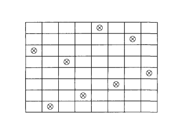
In other words, the $n$-tuples correspond to all possible placements of $n$ rooks on an $n \times n$ chessboard so that no two of them hit each other.
组合学代考
数学代写|组合学代写Combinatorics代考|Generating Function of Permutations by Inversions
在1.1节中,我们研究了排列的下降。也就是说,我们研究了排列中的一个条目大于它后面的条目的实例。一个更“全局”的排列统计是逆序统计。此统计信息将查找排列中的某个条目小于其后的某个条目(不一定直接)的实例。
定义2.1设$p=p_1 p_2 \cdots p_n$为一个排列。我们说$\left(p_i, p_j\right)$是$p$的反转,如果$ip_j$。
例2.2
排列31524有四个倒位,分别是$(3,1),(3,2),(5,2)$和$(5,4)$。
这方面的研究早在1901年就开始了[254]。在本节中,我们将调查这一领域中一些最有趣的结果。$p$的反转次数将用$i(p)$表示,尽管有些作者更喜欢$i n v(p)$。很明显,$0 \leq i(p) \leq\left(\begin{array}{c}n \ 2\end{array}\right)$适用于所有$n$ -排列,两个极值分别由$12 \cdots n$和$n(n-1) \cdots 1$排列获得。相对容易找到列出长度为$n$的所有排列的生成函数,相对于它们的反转次数。
定理2.3
对于所有正整数$n \geq 2$,
$$
\sum_{p \in S_n} z^{i(p)}=I_n(z)=(1+z)\left(1+z+z^2\right) \cdots\left(1+z+z^2+\cdots+z^{n-1}\right) .
$$
我们在$n$上用归纳法证明了这个命题。事实上,我们证明了每个$n$ !乘积$I_n(z)$的展开项正好对应于$S_n$中的一个排列。此外,展开项$z^{a_1} z^{a_2} \cdots z^{a_{n-1}}$将对应于唯一的排列,其中对于每个$i \in[n]$,条目$i+1$正好位于比其本身小的条目$a_i$之前。
如果是$n=2$,那么有两个排列要计数,$p=12$没有反转,$p^{\prime}=21$有一个反转。所以说$\sum_{p \in S_2} z^{i(p)}=1+z$。其中,$p=12$由展开项1表示,$p^{\prime}=21$由展开项$z$表示。
数学代写|组合学代写Combinatorics代考|Explicit Definition of Determinants
有一些本科数学课程和教科书只给出了方阵行列式的递归定义。也就是说,$\operatorname{det}\left(\begin{array}{ll}a & b \ c & d\end{array}\right)$被定义为等于$a d-b c$,那么$n \times n$矩阵$A=\left(a_{i j}\right)$的行列式被定义为
$$
\operatorname{det} A=\sum_{j=1}^n(-1)^{j-1} a_{1 j} A_{1 j}
$$
其中$A_{1 j}$是通过删除第一行和$j$第th列从$A$获得的$(n-1) \times(n-1)$矩阵。
如果这是读者所见过的行列式的唯一定义,他可能会发现下面的结果很有趣。
定理2.21
设$A=\left(a_{i j}\right)$为$n \times n$矩阵。然后我们有
$$
\operatorname{det} A=\sum_{p \in S_n}(-1)^{i(p)} a_{1 p_1} a_{2 p_2} \cdots a_{n p_n} .
$$
也就是说,$\operatorname{det} A$是全部取$n$得到的!可能的$n$ -元组的条目,以便在每行和每列中正好有一个$n$条目,将每个这样的$n$ -元组的元素相乘,最后取这些的带符号的和$n$ !其中的符号由$i(p)$的奇偶性决定,而$p$是由每个选择的$n$ -元组决定的排列。
换句话说,$n$ -元组对应于$n \times n$棋盘上$n$车的所有可能位置,这样它们就不会撞到对方。

统计代写请认准statistics-lab™. statistics-lab™为您的留学生涯保驾护航。
金融工程代写
金融工程是使用数学技术来解决金融问题。金融工程使用计算机科学、统计学、经济学和应用数学领域的工具和知识来解决当前的金融问题,以及设计新的和创新的金融产品。
非参数统计代写
非参数统计指的是一种统计方法,其中不假设数据来自于由少数参数决定的规定模型;这种模型的例子包括正态分布模型和线性回归模型。
广义线性模型代考
广义线性模型(GLM)归属统计学领域,是一种应用灵活的线性回归模型。该模型允许因变量的偏差分布有除了正态分布之外的其它分布。
术语 广义线性模型(GLM)通常是指给定连续和/或分类预测因素的连续响应变量的常规线性回归模型。它包括多元线性回归,以及方差分析和方差分析(仅含固定效应)。
有限元方法代写
有限元方法(FEM)是一种流行的方法,用于数值解决工程和数学建模中出现的微分方程。典型的问题领域包括结构分析、传热、流体流动、质量运输和电磁势等传统领域。
有限元是一种通用的数值方法,用于解决两个或三个空间变量的偏微分方程(即一些边界值问题)。为了解决一个问题,有限元将一个大系统细分为更小、更简单的部分,称为有限元。这是通过在空间维度上的特定空间离散化来实现的,它是通过构建对象的网格来实现的:用于求解的数值域,它有有限数量的点。边界值问题的有限元方法表述最终导致一个代数方程组。该方法在域上对未知函数进行逼近。[1] 然后将模拟这些有限元的简单方程组合成一个更大的方程系统,以模拟整个问题。然后,有限元通过变化微积分使相关的误差函数最小化来逼近一个解决方案。
tatistics-lab作为专业的留学生服务机构,多年来已为美国、英国、加拿大、澳洲等留学热门地的学生提供专业的学术服务,包括但不限于Essay代写,Assignment代写,Dissertation代写,Report代写,小组作业代写,Proposal代写,Paper代写,Presentation代写,计算机作业代写,论文修改和润色,网课代做,exam代考等等。写作范围涵盖高中,本科,研究生等海外留学全阶段,辐射金融,经济学,会计学,审计学,管理学等全球99%专业科目。写作团队既有专业英语母语作者,也有海外名校硕博留学生,每位写作老师都拥有过硬的语言能力,专业的学科背景和学术写作经验。我们承诺100%原创,100%专业,100%准时,100%满意。
随机分析代写
随机微积分是数学的一个分支,对随机过程进行操作。它允许为随机过程的积分定义一个关于随机过程的一致的积分理论。这个领域是由日本数学家伊藤清在第二次世界大战期间创建并开始的。
时间序列分析代写
随机过程,是依赖于参数的一组随机变量的全体,参数通常是时间。 随机变量是随机现象的数量表现,其时间序列是一组按照时间发生先后顺序进行排列的数据点序列。通常一组时间序列的时间间隔为一恒定值(如1秒,5分钟,12小时,7天,1年),因此时间序列可以作为离散时间数据进行分析处理。研究时间序列数据的意义在于现实中,往往需要研究某个事物其随时间发展变化的规律。这就需要通过研究该事物过去发展的历史记录,以得到其自身发展的规律。
回归分析代写
多元回归分析渐进(Multiple Regression Analysis Asymptotics)属于计量经济学领域,主要是一种数学上的统计分析方法,可以分析复杂情况下各影响因素的数学关系,在自然科学、社会和经济学等多个领域内应用广泛。
MATLAB代写
MATLAB 是一种用于技术计算的高性能语言。它将计算、可视化和编程集成在一个易于使用的环境中,其中问题和解决方案以熟悉的数学符号表示。典型用途包括:数学和计算算法开发建模、仿真和原型制作数据分析、探索和可视化科学和工程图形应用程序开发,包括图形用户界面构建MATLAB 是一个交互式系统,其基本数据元素是一个不需要维度的数组。这使您可以解决许多技术计算问题,尤其是那些具有矩阵和向量公式的问题,而只需用 C 或 Fortran 等标量非交互式语言编写程序所需的时间的一小部分。MATLAB 名称代表矩阵实验室。MATLAB 最初的编写目的是提供对由 LINPACK 和 EISPACK 项目开发的矩阵软件的轻松访问,这两个项目共同代表了矩阵计算软件的最新技术。MATLAB 经过多年的发展,得到了许多用户的投入。在大学环境中,它是数学、工程和科学入门和高级课程的标准教学工具。在工业领域,MATLAB 是高效研究、开发和分析的首选工具。MATLAB 具有一系列称为工具箱的特定于应用程序的解决方案。对于大多数 MATLAB 用户来说非常重要,工具箱允许您学习和应用专业技术。工具箱是 MATLAB 函数(M 文件)的综合集合,可扩展 MATLAB 环境以解决特定类别的问题。可用工具箱的领域包括信号处理、控制系统、神经网络、模糊逻辑、小波、仿真等。