如果你也在 怎样代写最优控制optimal control这个学科遇到相关的难题，请随时右上角联系我们的24/7代写客服。

最优控制是为一个动态系统确定一段时期内的控制和状态轨迹，以使性能指数最小化的过程。

statistics-lab™ 为您的留学生涯保驾护航 在代写最优控制optimal control方面已经树立了自己的口碑, 保证靠谱, 高质且原创的统计Statistics代写服务。我们的专家在代写最优控制optimal control代写方面经验极为丰富，各种代写最优控制Soptimal control相关的作业也就用不着说。

我们提供的最优控制optimal control及其相关学科的代写，服务范围广, 其中包括但不限于:

• Statistical Inference 统计推断
• Statistical Computing 统计计算
• Advanced Probability Theory 高等楖率论
• Advanced Mathematical Statistics 高等数理统计学
• (Generalized) Linear Models 广义线性模型
• Statistical Machine Learning 统计机器学习
• Longitudinal Data Analysis 纵向数据分析
• Foundations of Data Science 数据科学基础

统计代写|最优控制作业代写optimal control代考|Calculus of Variations

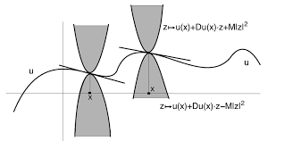
We begin now the analysis of some optimization problems where the results about semiconcave functions and their singularities can be applied. In this chapter we consider what Fleming and Rishel [80] call “the simplest problem in the calculus of variations,” a case where the dynamic programming approach is particularly powerful, and which will serve as a guideline for the analysis of optimal control problems in the following.

The problem in the calculus of variations we study here has been introduced in Chapter 1, where some results have been given in the case where the integrand is independent of $t, x$. Here, we consider a general integrand, so that the minimizers no longer admit an explicit description as in the Hopf formula. However, the structure of minimizers is described by classical results: we give a result about existence and regularity of minimizers, and we show that they satisfy the well-known Euler-Lagrange equations. We then apply the dynamic programming approach and introduce the value function of the problem, which is semiconcave and is a viscosity solution of an associated Hamilton-Jacobi equation. The main purpose of our analysis is to study the singularities of the value function and their interpretation in the calculus of variations. For instance, we derive a correspondence between generalized gradients of the value function and the minimizing trajectories of the problem. This shows, in particular, that the singularities of the value function are exactly the endpoints for which the minimizer of the variational problem is not unique. In addition, we can bound the size of $\bar{\Sigma}$, the closure of the singular set, proving that it enjoys the same rectifiability properties of $\Sigma$ itself. This result is interesting because on the complement of $\bar{\Sigma}$ the value function has the same regularity as the data and can be computed by the method of characteristics.

The chapter is organized as follows. In Section $6.1$ we give the statement of the problem and the existence result for minimizers. In Section $6.2$ we show that minimizers are regular and derive the Euler-Lagrange equations. Starting from Section $6.3$ we focus our attention on problems with one free endpoint; we introduce the notions of irregular and conjugate point and we prove Jacobi’s necessary optimality condition. Then, in Section 6.4, we apply the dynamic programming approach to this problem. We show that the value function $u$ solves the associated Hamilton-Jacobi

equation in the viscosity sense and that it is semiconcave. In addition, the minimizers for the variational problem with a given final endpoint $(t, x)$ are in one-to-one correspondence with the elements of $D^{*} u(t, x)$; in particular, the differentiability of $u$ is equivalent to the uniqueness of the minimizer. We also show that $u$ is as regular as the data of the problem in the complement of the closure of its singular set $\Sigma$.
The rest of the chapter is devoted to study the structure of $\bar{\Sigma}$. Since the properties of $\Sigma$ are well known from the general analysis of Chapter 4 , we focus our attention on the set $\bar{\Sigma} \backslash \Sigma$. The starting point is given in Section $6.5$, where we show that $\bar{\Sigma}=\Sigma \cup \Gamma$, where $\Gamma$ is the set of conjugate points. In addition, we prove some results about conjugate points showing, roughly speaking, that these are the points at which the singularities of $u$ are generated. Then, in Section $6.6$, we prove that $\Sigma$ has the same rectifiability property as $\Sigma$, i.e., it is a countably $\mathcal{H}^{\prime n}$-rectifiable subset of $\mathbb{R} \times \mathbb{R}^{n}$. By the previous remarks, this is equivalent to proving the rectifiability of $\Gamma \backslash \Sigma$. Combining a careful analysis of the hamiltonian system satisfied by the minimizing arcs with some tools from geometric measure theory, we obtain the finer estimate
$$
\mathcal{H}^{n-1+\frac{2}{R-1}}(\Gamma \backslash \Sigma)=0,
$$
where $k \geq 3$ is the differentiability class of the data. This yields in particular the desired Hausdorff estimate on $\bar{\Sigma}$, which shows that $u$ is as smooth as the data in the complement of a closed rectifiable set of codimension one.

统计代写|最优控制作业代写optimal control代考|Existence of minimizers

Let us consider the problem in the calculus of variations of Chapter 1 in a more general setting. We fix $T>0$, a connected open set $\Omega \subset \mathbb{R}^{n}$ and two closed subsets $S_{0}, S_{T} \subset \bar{\Omega}$. We denote by $\mathrm{AC}\left([0, T], \mathbb{R}^{n}\right)$ the class of all absolutely continuous arcs $\xi:[0, T] \rightarrow \mathbb{R}^{n}$ and define the set of admissible arcs by
$$
\mathcal{A}=\left{\xi \in \mathrm{AC}\left([0, T], \mathbb{R}^{n}\right): \xi(t) \in \bar{\Omega} \text { for all } t \in[0, T], \xi(0) \in S_{0}, \xi(T) \in S_{T}\right}
$$
Moreover, we define the functionals $\Lambda, J$ on $\mathcal{A}$ by
$$
\Lambda(\xi)=\int_{0}^{T} L(s, \xi(s), \dot{\xi}(s)) d s
$$
and
$$
J(\xi)=\Lambda(\xi)+u_{0}(\xi(0))+u_{T}(\xi(T))
$$
Here $L:[0, T] \times \bar{\Omega} \times \mathbb{R}^{n} \rightarrow \mathbb{R}$ and $u_{0}, u_{T}: \bar{\Omega} \rightarrow \mathbb{R}$ are given continuous functions called running cost, initial cost and final cost, respectively, and $\Lambda$ is the action functional. We then consider the following minimization problem:
(CV) Find $\xi_{} \in \mathcal{A}$ such that $J\left(\xi_{}\right)=\min {J(\xi): \xi \in \mathcal{A}}$.

统计代写|最优控制作业代写optimal control代考|Necessary conditions and regularity

We show in this section that the minimizing arcs for problem (CV) are regular and solve a system of equations called the Euler-Lagrange equations. Our analysis is restricted to those minimizers which are contained in $\Omega$; minimizers touching the boundary of $\Omega$ would require a longer analysis. We need some further assumptions on the data. Namely, we assume that the lagrangian $L$ is of class $C^{1}$ and that for all $r>0$ there exists $\mathcal{C}(r)>0$ such that
$$
\begin{aligned}
&\left|L_{x}(t, x, v)\right|+\left|L_{v}(t, x, v)\right| \leq \tilde{C}(r) \theta(|v|) \
&\forall t \in[0, T], x \in \bar{\Omega} \cap B_{r}, v \in \mathbb{R}^{n}
\end{aligned}
$$
where $\theta$ is the Nagumo function appearing in hypothesis (ii) of Theorem 6.1.2. Observe that property (iii) of the same theorem is implied by (6.6). In addition, we assume that $\theta$ satisfies
$$
\theta(q+m) \leq K_{M}[1+\theta(q)] \quad \forall m \in[0, M], q \geq 0
$$
It is easily checked that assumption (6.7) is satisfied for many classes of superlinear functions $\theta$, such as powers or exponentials. It is violated in cases where $\theta$ grows “very fast”, e.g., $\theta(q)=e^{e q}, q \in \mathbb{R}$.

最优控制代考

统计代写|最优控制作业代写optimal control代考|Calculus of Variations

我们现在开始分析一些可以应用半凹函数及其奇异性的结果的优化问题。在本章中，我们考虑 Fleming 和 Rishel [80] 所说的“变分计算中最简单的问题”，这是动态规划方法特别强大的一种情况，它将作为分析最优控制问题的指南。以下。

我们在此处研究的变分计算问题已在第 1 章中介绍过，其中在被积函数独立于吨,X. 在这里，我们考虑一个一般被积函数，因此最小化器不再允许像 Hopf 公式中那样的明确描述。然而，最小化器的结构是由经典结果描述的：我们给出了最小化器的存在性和规律性的结果，并且我们证明了它们满足著名的欧拉-拉格朗日方程。然后我们应用动态规划方法并引入问题的价值函数，它是半凹的，是相关 Hamilton-Jacobi 方程的粘度解。我们分析的主要目的是研究价值函数的奇异性及其在变分法中的解释。例如，我们推导出值函数的广义梯度与问题的最小化轨迹之间的对应关系。这尤其表明，值函数的奇点正是变分问题的最小化器不是唯一的端点。此外，我们可以限制Σ¯，奇异集的闭包，证明它具有相同的可整流性质Σ本身。这个结果很有趣，因为在Σ¯值函数与数据具有相同的规律性，可以通过特征法计算。

本章组织如下。在部分6.1我们给出了问题的陈述和最小化器的存在结果。在部分6.2我们证明了最小化器是规则的并推导出欧拉-拉格朗日方程。从节开始6.3我们将注意力集中在一个免费端点的问题上；我们引入了不规则点和共轭点的概念，并证明了 Jacobi 的必要最优性条件。然后，在第 6.4 节中，我们将动态规划方法应用于这个问题。我们证明了价值函数在求解相关的 Hamilton-Jacobi

在粘度意义上的方程，它是半凹的。此外，具有给定最终端点的变分问题的最小化器(吨,X)与元素一一对应D∗在(吨,X); 特别是，可区分性在等价于最小化器的唯一性。我们还表明在与问题的数据在其奇异集的闭包的补中一样规则Σ.
本章的其余部分专门研究结构Σ¯. 由于属性Σ从第 4 章的一般分析中众所周知，我们将注意力集中在集合上Σ¯∖Σ. 起点在章节中给出6.5, 我们证明Σ¯=Σ∪Γ， 在哪里Γ是共轭点的集合。此外，我们证明了一些关于共轭点的结果，粗略地说，这些是在被生成。然后，在部分6.6, 我们证明Σ具有与Σ, 即它是一个可数的H′n-可纠正的子集R×Rn. 通过前面的评论，这相当于证明了Γ∖Σ. 结合对最小化弧所满足的哈密顿系统的仔细分析与几何测度理论中的一些工具，我们得到了更精细的估计
Hn−1+2R−1(Γ∖Σ)=0,
在哪里ķ≥3是数据的可微性类别。这特别产生了所需的豪斯多夫估计Σ¯，这表明在与封闭的可校正余维集补集中的数据一样平滑。

统计代写|最优控制作业代写optimal control代考|Existence of minimizers

让我们在更一般的背景下考虑第 1 章变分法中的问题。我们修复吨>0, 连通开集Ω⊂Rn和两个封闭子集小号0,小号吨⊂Ω¯. 我们表示一种C([0,吨],Rn)所有绝对连续弧的类X:[0,吨]→Rn并通过以下方式定义允许弧的集合
\mathcal{A}=\left{\xi \in \mathrm{AC}\left([0, T], \mathbb{R}^{n}\right): \xi(t) \in \bar{ \Omega} \text { 对于所有 } t \in[0, T], \xi(0) \in S_{0}, \xi(T) \in S_{T}\right}\mathcal{A}=\left{\xi \in \mathrm{AC}\left([0, T], \mathbb{R}^{n}\right): \xi(t) \in \bar{ \Omega} \text { 对于所有 } t \in[0, T], \xi(0) \in S_{0}, \xi(T) \in S_{T}\right}
此外，我们定义泛函Λ,Ĵ在一种经过
Λ(X)=∫0吨大号(s,X(s),X˙(s))ds
和
Ĵ(X)=Λ(X)+在0(X(0))+在吨(X(吨))
这里大号:[0,吨]×Ω¯×Rn→R和在0,在吨:Ω¯→R给定连续函数，分别称为运行成本、初始成本和最终成本，并且Λ是动作泛函。然后我们考虑以下最小化问题：
(CV) FindX∈一种这样Ĵ(X)=分钟Ĵ(X):X∈一种.

统计代写|最优控制作业代写optimal control代考|Necessary conditions and regularity

我们在本节中展示了问题 (CV) 的最小化弧是规则的，并求解了一个称为 Euler-Lagrange 方程的方程组。我们的分析仅限于那些包含在Ω; 接触边界的最小化器Ω将需要更长的分析时间。我们需要对数据做一些进一步的假设。即，我们假设拉格朗日大号是一流的C1这对所有人r>0那里存在C(r)>0这样
|大号X(吨,X,在)|+|大号在(吨,X,在)|≤C~(r)θ(|在|) ∀吨∈[0,吨],X∈Ω¯∩乙r,在∈Rn
在哪里θ是出现在定理 6.1.2 的假设 (ii) 中的 Nagumo 函数。观察同一定理的性质 (iii) 由 (6.6) 暗示。此外，我们假设θ满足
θ(q+米)≤ķ米[1+θ(q)]∀米∈[0,米],q≥0
很容易检查假设（6.7）对于许多类别的超线性函数都满足θ，例如幂或指数。它在以下情况下被违反θ增长“非常快”，例如，θ(q)=和和q,q∈R.

统计代写请认准statistics-lab™. statistics-lab™为您的留学生涯保驾护航。

金融工程代写

金融工程是使用数学技术来解决金融问题。金融工程使用计算机科学、统计学、经济学和应用数学领域的工具和知识来解决当前的金融问题，以及设计新的和创新的金融产品。

非参数统计代写

非参数统计指的是一种统计方法，其中不假设数据来自于由少数参数决定的规定模型；这种模型的例子包括正态分布模型和线性回归模型。

广义线性模型代考

广义线性模型（GLM）归属统计学领域，是一种应用灵活的线性回归模型。该模型允许因变量的偏差分布有除了正态分布之外的其它分布。

术语 广义线性模型（GLM）通常是指给定连续和/或分类预测因素的连续响应变量的常规线性回归模型。它包括多元线性回归，以及方差分析和方差分析（仅含固定效应）。

有限元方法代写

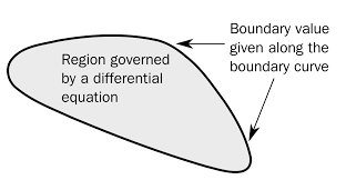
有限元方法（FEM）是一种流行的方法，用于数值解决工程和数学建模中出现的微分方程。典型的问题领域包括结构分析、传热、流体流动、质量运输和电磁势等传统领域。

有限元是一种通用的数值方法，用于解决两个或三个空间变量的偏微分方程（即一些边界值问题）。为了解决一个问题，有限元将一个大系统细分为更小、更简单的部分，称为有限元。这是通过在空间维度上的特定空间离散化来实现的，它是通过构建对象的网格来实现的：用于求解的数值域，它有有限数量的点。边界值问题的有限元方法表述最终导致一个代数方程组。该方法在域上对未知函数进行逼近。[1] 然后将模拟这些有限元的简单方程组合成一个更大的方程系统，以模拟整个问题。然后，有限元通过变化微积分使相关的误差函数最小化来逼近一个解决方案。

tatistics-lab作为专业的留学生服务机构，多年来已为美国、英国、加拿大、澳洲等留学热门地的学生提供专业的学术服务，包括但不限于Essay代写，Assignment代写，Dissertation代写，Report代写，小组作业代写，Proposal代写，Paper代写，Presentation代写，计算机作业代写，论文修改和润色，网课代做，exam代考等等。写作范围涵盖高中，本科，研究生等海外留学全阶段，辐射金融，经济学，会计学，审计学，管理学等全球99%专业科目。写作团队既有专业英语母语作者，也有海外名校硕博留学生，每位写作老师都拥有过硬的语言能力，专业的学科背景和学术写作经验。我们承诺100%原创，100%专业，100%准时，100%满意。

随机分析代写

随机微积分是数学的一个分支，对随机过程进行操作。它允许为随机过程的积分定义一个关于随机过程的一致的积分理论。这个领域是由日本数学家伊藤清在第二次世界大战期间创建并开始的。

时间序列分析代写

随机过程，是依赖于参数的一组随机变量的全体，参数通常是时间。 随机变量是随机现象的数量表现，其时间序列是一组按照时间发生先后顺序进行排列的数据点序列。通常一组时间序列的时间间隔为一恒定值（如1秒，5分钟，12小时，7天，1年），因此时间序列可以作为离散时间数据进行分析处理。研究时间序列数据的意义在于现实中，往往需要研究某个事物其随时间发展变化的规律。这就需要通过研究该事物过去发展的历史记录，以得到其自身发展的规律。

回归分析代写

多元回归分析渐进（Multiple Regression Analysis Asymptotics）属于计量经济学领域，主要是一种数学上的统计分析方法，可以分析复杂情况下各影响因素的数学关系，在自然科学、社会和经济学等多个领域内应用广泛。

MATLAB代写

MATLAB 是一种用于技术计算的高性能语言。它将计算、可视化和编程集成在一个易于使用的环境中，其中问题和解决方案以熟悉的数学符号表示。典型用途包括：数学和计算算法开发建模、仿真和原型制作数据分析、探索和可视化科学和工程图形应用程序开发，包括图形用户界面构建MATLAB 是一个交互式系统，其基本数据元素是一个不需要维度的数组。这使您可以解决许多技术计算问题，尤其是那些具有矩阵和向量公式的问题，而只需用 C 或 Fortran 等标量非交互式语言编写程序所需的时间的一小部分。MATLAB 名称代表矩阵实验室。MATLAB 最初的编写目的是提供对由 LINPACK 和 EISPACK 项目开发的矩阵软件的轻松访问，这两个项目共同代表了矩阵计算软件的最新技术。MATLAB 经过多年的发展，得到了许多用户的投入。在大学环境中，它是数学、工程和科学入门和高级课程的标准教学工具。在工业领域，MATLAB 是高效研究、开发和分析的首选工具。MATLAB 具有一系列称为工具箱的特定于应用程序的解决方案。对于大多数 MATLAB 用户来说非常重要，工具箱允许您学习和应用专业技术。工具箱是 MATLAB 函数（M 文件）的综合集合，可扩展 MATLAB 环境以解决特定类别的问题。可用工具箱的领域包括信号处理、控制系统、神经网络、模糊逻辑、小波、仿真等。

R语言代写	问卷设计与分析代写
PYTHON代写	回归分析与线性模型代写
MATLAB代写	方差分析与试验设计代写
STATA代写	机器学习/统计学习代写
SPSS代写	计量经济学代写
EVIEWS代写	时间序列分析代写
EXCEL代写	深度学习代写
SQL代写	各种数据建模与可视化代写

如果你也在 怎样代写最优控制optimal control这个学科遇到相关的难题，请随时右上角联系我们的24/7代写客服。

最优控制是为一个动态系统确定一段时期内的控制和状态轨迹，以使性能指数最小化的过程。

statistics-lab™ 为您的留学生涯保驾护航 在代写最优控制optimal control方面已经树立了自己的口碑, 保证靠谱, 高质且原创的统计Statistics代写服务。我们的专家在代写最优控制optimal control代写方面经验极为丰富，各种代写最优控制Soptimal control相关的作业也就用不着说。

我们提供的最优控制optimal control及其相关学科的代写，服务范围广, 其中包括但不限于:

• Statistical Inference 统计推断
• Statistical Computing 统计计算
• Advanced Probability Theory 高等楖率论
• Advanced Mathematical Statistics 高等数理统计学
• (Generalized) Linear Models 广义线性模型
• Statistical Machine Learning 统计机器学习
• Longitudinal Data Analysis 纵向数据分析
• Foundations of Data Science 数据科学基础

统计代写|最优控制作业代写optimal control代考|Viscosity solutions

Let $\Omega \subset \mathbb{R}^{n}$ be an open set and let $H \in C\left(\Omega \times \mathbb{R} \times \mathbb{R}^{n}\right)$. Let us again consider the general nonlinear first order equation
$$
H(x, u, D u)=0, \quad x \in \Omega \subset \mathbb{R}^{n},
$$
in the unknown $u: \Omega \rightarrow \mathbb{R}$. As usual, evolution equations can be recast in this form by considering time as an additional space variable.

As we have already mentioned, when one considers boundary value problems or Cauchy problems for equations of the above form, one finds that in general no global smooth solutions exist even if the data are smooth. On the other hand, the property of being a Lipschitz continuous function satisfying the equation almost everywhere is usually too weak to have uniqueness results. Therefore, a crucial step in the analysis is to give a notion of a generalized solution such that global existence and uniqueness results can be obtained. In Chapter 1 we have seen a class of problems which are well posed in the class of semiconcave solutions. Here we present the notion of a viscosity solution, which has a much wider range of applicability.

Definition 5.2.1 A function $u \in C(\Omega)$ is called a viscosity subsolution of equation (5.14) if, for any $x \in \Omega$, it satisfies
$$
H(x, u(x), p) \leq 0, \quad \forall p \in D^{+} u(x) .
$$
Similarly, we say that $u$ is a viscosity supersolution of equation (5.14) if, for any $x \in \Omega$, we have
$$
H(x, u(x), p) \geq 0, \quad \forall p \in D^{-} u(x)
$$
If u satisfies both of the above properties, it is called a viscosity solution of equation (5.14).

Observe that, by virtue of Proposition 3.1.7, condition (5.15) (resp. (5.16)) can be restated in an equivalent way by requiring
$$
H(x, u(x), D \phi(x)) \leq 0 \quad \text { (resp. } H(x, u(x), D \phi(x)) \geq 0 \text { ) }
$$
for any $\phi \in C^{1}(\Omega)$ such that $u-\phi$ has a local maximum (resp. minimum) at $x$.
We see that if $u$ is differentiable everywhere the notion of a viscosity solution coincides with the classical one since we have at any point $D^{+} u(x)=D^{-} u(x)=$ ${D u(x)}$. On the other hand, if $u$ is not differentiable everywhere, the definition of a viscosity solution includes additional requirements at the points of nondifferentiability. The reason for taking inequalities (5.15)-(5.16) as the definition of solution might not be clear at first sight, as well as the relation with the semiconcavity property considered in Chapter 1 . However, we will see that with this definition one can obtain existence and uniqueness results for many classes of Hamilton-Jacobi equations, and that the viscosity solution usually coincides with the one which is relevant for the applications, like the value function in optimal control. The relationship with semiconcavity will be examined in detail in the next section.

统计代写|最优控制作业代写optimal control代考|Semiconcavity and viscosity

We now analyze the relation between the notions of a semiconcave solution and a viscosity solution to Hamilton-Jacobi equations. We will see that the two notions are strictly related when the hamiltonian is a convex function of $D u$. We begin with the following result.

Proposition $5.3 .1$ Let u be a semiconcave function satisfying equation (5.14) almost everywhere. If $H$ is convex in the third argument, then $u$ is a viscosity solution of the equation.

Proof – As a first step. we show that $u$ satisfies the equation at all points of differentiability (our assumption is a priori slightly weaker). Let $u$ be differentiable at some $x_{0} \in \Omega$. Then there exists a sequence of points $x_{k}$ converging to $x_{0}$ such that
(i) $u$ is differentiable at $x_{k}$;
(ii) $H\left(x_{k}, u\left(x_{k}\right), D u\left(x_{k}\right)\right)=0$;
(iii) $D u\left(x_{k}\right)$ has a limit for $k \rightarrow \infty$.
From Proposition 3.3.4(a) we deduce that the limit of $D u\left(x_{k}\right)$ is $D u\left(x_{0}\right)$. By the continuity of $H$, the equation holds at $x_{0}$ as well.

Let us now take an arbitrary $x \in \Omega$ and check that (5.15) is satisfied. We first observe that
$$
H(x, u(x), p)=0, \quad \forall p \in D^{} u(x) $$ This follows directly from the definition of $D^{} u$, the continuity of $H$ and the property that the equation holds at the points of differentiability. Since $D^{+} u(x)$ is the convex hull of $D^{*} u(x)$ (see Theorem $3.3 .6$ ) and $H$ is convex, inequality (5.15) follows.
Now let us check inequality (5.16). For a given $x \in \Omega$, suppose that $D^{-} u(x)$ contains some vector $p$. Then, by Proposition 3.1.5(c) and Proposition 3.3.4(c), $u$ is differentiable at $x$ and $D u(x)=p$. Thus, $(5.16)$ holds as an equality by the first part of the proof.

Remark 5.3.2 A more careful analysis shows that the convexity of $H$ and the semiconcavity of $u$ play independent roles in the viscosity property. In fact, in the previous proof, the deduction that $u$ is a supersolution uses only semiconcavity and is valid also if $H$ is not convex. On the other hand, it is possible to prove (see see [110, p. 96] or [20, Prop. II.5.1]) that, if $H$ is convex, any Lipschitz continuous $u$ (not necessarily semiconcave) satisfying the equation almost everywhere is a viscosity subsolution of the equation.

统计代写|最优控制作业代写optimal control代考|Propagation of singularities

We now turn to the analysis of the singular set of semiconcave solutions to HamiltonJacobi equations. In Chapter 4 we have obtained results which are valid for any semiconcave function; here we focus our attention on semiconcave functions which are solutions to Hamilton-Jacobi equations and we obtain stronger results on the propagation of singularities in this case. As in the previous chapter, our discussion is restricted to semiconcave functions with linear modulus (some results in the case of a general modulus can be found in [1]).
We consider again an equation of the form
$$
F(x, u(x), D u(x))=0 \quad \text { a.e. in } \quad \Omega
$$
Throughout the rest of this chapter, $F: \bar{\Omega} \times \mathbb{R} \times \mathbb{R}^{n} \rightarrow \mathbb{R}$ is a continuous function satisfying the following assumptions:
(Al) $p \mapsto F(x, u, p)$ is convex;
(A2) for any $(x, u) \in \Omega \times \mathbb{R}$ and any $p_{0}, p_{1} \in \mathbb{R}^{n}$,
$$
\left\lfloor p_{0}, p_{1}\right] \subset\left{p \in \mathbb{R}^{n}: F(x, u, p)=0\right} \quad \Longrightarrow \quad p_{0}=p_{1} .
$$
Condition (A2) requires that the 0 -level set $\left{p \in \mathbb{R}^{n}: F(x, u, p)=0\right}$ contains no straight line. Clearly, such a property holds, in particular, if $F$ is strictly convex with respect to $p$. Observe, however, that it also holds for functions like $F(x, u, p)=|p|$ which are not strictly convex.

Remark 5.4.1 In Proposition 5.3.1 we have seen that, under the convexity assumption (A1), any semiconcave function $u$ which solves equation (5.44) almost everywhere is also a viscosity solution of the equation. Thus, $u$ satisfies for all $x \in \Omega$
$$
\begin{array}{ll}
F(x, u(x), p)=0 & \forall p \in D^{*} u(x) \
F(x, u(x), p) \leq 0 & \forall p \in D^{+} u(x)
\end{array}
$$
The first result we prove is that condition (4.8) is necessary and sufficient for the propagation of a singularity at $x_{0}$, if $u$ is a semiconcave solution of (5.44). Notice that, for a general semiconcave function, (4.8) is only a sufficient condition.

Theorem 5.4.2 Let (A1) and (A2) be satisfied. Let $u \in \mathrm{SCL}{l o c}(\Omega)$ be a solution of (5.44) and let $x{0} \in \Sigma(u)$. Then, the following properties are equivalent:
(i) $\partial D^{+} u\left(x_{0}\right) \backslash D^{*} u\left(x_{0}\right) \neq \emptyset$;
(ii) there exist a sequence $x_{i} \in \Sigma(u) \backslash\left{x_{0}\right}$, converging to $x_{0}$, and a number $\delta>0$ such that diam $D^{+} u\left(x_{i}\right) \geq \delta$, for any $i \in \mathbb{N}$.

最优控制代考

统计代写|最优控制作业代写optimal control代考|Viscosity solutions

让Ω⊂Rn是一个开集并且让H∈C(Ω×R×Rn). 让我们再次考虑一般的非线性一阶方程
H(X,在,D在)=0,X∈Ω⊂Rn,
在未知的在:Ω→R. 像往常一样，通过将时间视为额外的空间变量，可以以这种形式重铸进化方程。

正如我们已经提到的，当考虑上述形式的方程的边值问题或柯西问题时，人们会发现即使数据是平滑的，通常也不存在全局平滑解。另一方面，作为几乎处处满足方程的 Lipschitz 连续函数的性质通常太弱而无法得到唯一性结果。因此，分析中的一个关键步骤是给出一个广义解的概念，以便可以获得全局存在性和唯一性结果。在第 1 章中，我们已经看到了在半凹解类中很好地提出的一类问题。在这里，我们提出了粘度解决方案的概念，它具有更广泛的适用性。

定义 5.2.1 一个函数在∈C(Ω)被称为方程（5.14）的粘度子解，如果，对于任何X∈Ω, 满足
H(X,在(X),p)≤0,∀p∈D+在(X).
同样，我们说在是方程 (5.14) 的粘度超解，如果，对于任何X∈Ω， 我们有
H(X,在(X),p)≥0,∀p∈D−在(X)
如果 u 满足上述两个性质，则称为方程（5.14）的粘度解。

观察到，根据命题 3.1.7，条件 (5.15) (resp. (5.16)) 可以通过要求以等价方式重述
H(X,在(X),Dφ(X))≤0 （分别。 H(X,在(X),Dφ(X))≥0 ) 
对于任何φ∈C1(Ω)这样在−φ有一个局部最大值（分别是最小值）在X.
我们看到，如果在处处可微 粘度解的概念与经典解的概念一致，因为我们在任何时候都有D+在(X)=D−在(X)= D在(X). 另一方面，如果在不是处处可微的，粘度解的定义包括在不可微点处的附加要求。将不等式(5.15)-(5.16)作为解定义的原因，乍一看可能不太清楚，以及与第1章考虑的半凹性质的关系。然而，我们将看到，通过这个定义，我们可以获得许多类别的 Hamilton-Jacobi 方程的存在性和唯一性结果，并且粘度解通常与与应用相关的解一致，例如最优控制中的值函数。与半凹度的关系将在下一节中详细研究。

统计代写|最优控制作业代写optimal control代考|Semiconcavity and viscosity

我们现在分析 Hamilton-Jacobi 方程的半凹解和粘度解的概念之间的关系。我们将看到，当哈密顿是一个凸函数时，这两个概念是严格相关的D在. 我们从以下结果开始。

主张5.3.1令 u 是几乎处处满足方程 (5.14) 的半凹函数。如果H在第三个参数中是凸的，那么在是方程的粘度解。

证明——作为第一步。我们证明了在在所有可微点处满足方程（我们的假设先验稍弱）。让在在某些方面是可区分的X0∈Ω. 那么存在点序列Xķ收敛到X0这样
(i)在可微分于Xķ;
(二)H(Xķ,在(Xķ),D在(Xķ))=0;
㈢D在(Xķ)有一个限制ķ→∞.
从命题 3.3.4(a) 我们推断出D在(Xķ)是D在(X0). 通过连续性H，等式在X0以及。

现在让我们任意取X∈Ω并检查 (5.15) 是否满足。我们首先观察到
H(X,在(X),p)=0,∀p∈D在(X)这直接来自于D在, 的连续性H以及等式在可微点处所具有的性质。自从D+在(X)是凸包D∗在(X)（见定理3.3.6） 和H是凸的，不等式（5.15）如下。
现在让我们检查不等式（5.16）。对于给定的X∈Ω, 假设D−在(X)包含一些向量p. 然后，根据提案 3.1.5(c) 和提案 3.3.4(c)，在可微分于X和D在(X)=p. 因此，(5.16)由证明的第一部分成立。

备注 5.3.2 更仔细的分析表明，H和半凹度在在粘度特性中起独立作用。事实上，在前面的证明中，推论在是一个超解仅使用半凹性并且如果H不是凸的。另一方面，有可能证明（见 [110, p. 96] 或 [20, Prop. II.5.1]），如果H是凸的，任何 Lipschitz 连续的在（不一定是半凹的）几乎处处满足方程是方程的粘度子解。

统计代写|最优控制作业代写optimal control代考|Propagation of singularities

我们现在转向分析 HamiltonJacobi 方程的奇异半凹解集。在第 4 章中，我们得到了对任何半凹函数都有效的结果；在这里，我们将注意力集中在半凹函数上，它是 Hamilton-Jacobi 方程的解，并且在这种情况下，我们在奇点的传播上获得了更强的结果。与前一章一样，我们的讨论仅限于具有线性模量的半凹函数（在 [1] 中可以找到一般模量情况下的一些结果）。
我们再次考虑以下形式的方程
F(X,在(X),D在(X))=0 一个和在 Ω
在本章的其余部分，F:Ω¯×R×Rn→R是满足以下假设的连续函数：
(Al)p↦F(X,在,p)是凸的；
(A2) 对于任何(X,在)∈Ω×R和任何p0,p1∈Rn,
\left\lfloor p_{0}, p_{1}\right] \subset\left{p \in \mathbb{R}^{n}: F(x, u, p)=0\right} \quad \ Longrightarrow \quad p_{0}=p_{1} 。\left\lfloor p_{0}, p_{1}\right] \subset\left{p \in \mathbb{R}^{n}: F(x, u, p)=0\right} \quad \ Longrightarrow \quad p_{0}=p_{1} 。
条件 (A2) 要求 0 水平集\left{p \in \mathbb{R}^{n}: F(x, u, p)=0\right}\left{p \in \mathbb{R}^{n}: F(x, u, p)=0\right}不包含直线。显然，这样的性质特别成立，如果F是严格凸的p. 但是请注意，它也适用于以下功能F(X,在,p)=|p|不是严格凸的。

备注 5.4.1 在命题 5.3.1 中，我们已经看到，在凸性假设 (A1) 下，任何半凹函数在几乎处处求解方程 (5.44) 也是方程的粘度解。因此，在满足所有人X∈Ω
F(X,在(X),p)=0∀p∈D∗在(X) F(X,在(X),p)≤0∀p∈D+在(X)
我们证明的第一个结果是条件（4.8）对于奇点在X0， 如果在是 (5.44) 的半凹解。请注意，对于一般半凹函数，(4.8) 只是一个充分条件。

定理 5.4.2 令 (A1) 和 (A2) 满足。让在∈小号C大号l这C(Ω)是 (5.44) 的解并让X0∈Σ(在). 那么，以下性质是等价的：
(i)∂D+在(X0)∖D∗在(X0)≠∅;
(ii) 存在一个序列x_{i} \in \Sigma(u) \backslash\left{x_{0}\right}x_{i} \in \Sigma(u) \backslash\left{x_{0}\right}, 收敛到X0, 和一个数字d>0这样直径D+在(X一世)≥d, 对于任何一世∈ñ.

统计代写请认准statistics-lab™. statistics-lab™为您的留学生涯保驾护航。

金融工程代写

金融工程是使用数学技术来解决金融问题。金融工程使用计算机科学、统计学、经济学和应用数学领域的工具和知识来解决当前的金融问题，以及设计新的和创新的金融产品。

非参数统计代写

非参数统计指的是一种统计方法，其中不假设数据来自于由少数参数决定的规定模型；这种模型的例子包括正态分布模型和线性回归模型。

广义线性模型代考

广义线性模型（GLM）归属统计学领域，是一种应用灵活的线性回归模型。该模型允许因变量的偏差分布有除了正态分布之外的其它分布。

术语 广义线性模型（GLM）通常是指给定连续和/或分类预测因素的连续响应变量的常规线性回归模型。它包括多元线性回归，以及方差分析和方差分析（仅含固定效应）。

有限元方法代写

有限元方法（FEM）是一种流行的方法，用于数值解决工程和数学建模中出现的微分方程。典型的问题领域包括结构分析、传热、流体流动、质量运输和电磁势等传统领域。

有限元是一种通用的数值方法，用于解决两个或三个空间变量的偏微分方程（即一些边界值问题）。为了解决一个问题，有限元将一个大系统细分为更小、更简单的部分，称为有限元。这是通过在空间维度上的特定空间离散化来实现的，它是通过构建对象的网格来实现的：用于求解的数值域，它有有限数量的点。边界值问题的有限元方法表述最终导致一个代数方程组。该方法在域上对未知函数进行逼近。[1] 然后将模拟这些有限元的简单方程组合成一个更大的方程系统，以模拟整个问题。然后，有限元通过变化微积分使相关的误差函数最小化来逼近一个解决方案。

tatistics-lab作为专业的留学生服务机构，多年来已为美国、英国、加拿大、澳洲等留学热门地的学生提供专业的学术服务，包括但不限于Essay代写，Assignment代写，Dissertation代写，Report代写，小组作业代写，Proposal代写，Paper代写，Presentation代写，计算机作业代写，论文修改和润色，网课代做，exam代考等等。写作范围涵盖高中，本科，研究生等海外留学全阶段，辐射金融，经济学，会计学，审计学，管理学等全球99%专业科目。写作团队既有专业英语母语作者，也有海外名校硕博留学生，每位写作老师都拥有过硬的语言能力，专业的学科背景和学术写作经验。我们承诺100%原创，100%专业，100%准时，100%满意。

随机分析代写

随机微积分是数学的一个分支，对随机过程进行操作。它允许为随机过程的积分定义一个关于随机过程的一致的积分理论。这个领域是由日本数学家伊藤清在第二次世界大战期间创建并开始的。

时间序列分析代写

随机过程，是依赖于参数的一组随机变量的全体，参数通常是时间。 随机变量是随机现象的数量表现，其时间序列是一组按照时间发生先后顺序进行排列的数据点序列。通常一组时间序列的时间间隔为一恒定值（如1秒，5分钟，12小时，7天，1年），因此时间序列可以作为离散时间数据进行分析处理。研究时间序列数据的意义在于现实中，往往需要研究某个事物其随时间发展变化的规律。这就需要通过研究该事物过去发展的历史记录，以得到其自身发展的规律。

回归分析代写

多元回归分析渐进（Multiple Regression Analysis Asymptotics）属于计量经济学领域，主要是一种数学上的统计分析方法，可以分析复杂情况下各影响因素的数学关系，在自然科学、社会和经济学等多个领域内应用广泛。

MATLAB代写

MATLAB 是一种用于技术计算的高性能语言。它将计算、可视化和编程集成在一个易于使用的环境中，其中问题和解决方案以熟悉的数学符号表示。典型用途包括：数学和计算算法开发建模、仿真和原型制作数据分析、探索和可视化科学和工程图形应用程序开发，包括图形用户界面构建MATLAB 是一个交互式系统，其基本数据元素是一个不需要维度的数组。这使您可以解决许多技术计算问题，尤其是那些具有矩阵和向量公式的问题，而只需用 C 或 Fortran 等标量非交互式语言编写程序所需的时间的一小部分。MATLAB 名称代表矩阵实验室。MATLAB 最初的编写目的是提供对由 LINPACK 和 EISPACK 项目开发的矩阵软件的轻松访问，这两个项目共同代表了矩阵计算软件的最新技术。MATLAB 经过多年的发展，得到了许多用户的投入。在大学环境中，它是数学、工程和科学入门和高级课程的标准教学工具。在工业领域，MATLAB 是高效研究、开发和分析的首选工具。MATLAB 具有一系列称为工具箱的特定于应用程序的解决方案。对于大多数 MATLAB 用户来说非常重要，工具箱允许您学习和应用专业技术。工具箱是 MATLAB 函数（M 文件）的综合集合，可扩展 MATLAB 环境以解决特定类别的问题。可用工具箱的领域包括信号处理、控制系统、神经网络、模糊逻辑、小波、仿真等。

R语言代写	问卷设计与分析代写
PYTHON代写	回归分析与线性模型代写
MATLAB代写	方差分析与试验设计代写
STATA代写	机器学习/统计学习代写
SPSS代写	计量经济学代写
EVIEWS代写	时间序列分析代写
EXCEL代写	深度学习代写
SQL代写	各种数据建模与可视化代写

如果你也在 怎样代写最优控制optimal control这个学科遇到相关的难题，请随时右上角联系我们的24/7代写客服。

最优控制是为一个动态系统确定一段时期内的控制和状态轨迹，以使性能指数最小化的过程。

statistics-lab™ 为您的留学生涯保驾护航 在代写最优控制optimal control方面已经树立了自己的口碑, 保证靠谱, 高质且原创的统计Statistics代写服务。我们的专家在代写最优控制optimal control代写方面经验极为丰富，各种代写最优控制Soptimal control相关的作业也就用不着说。

我们提供的最优控制optimal control及其相关学科的代写，服务范围广, 其中包括但不限于:

• Statistical Inference 统计推断
• Statistical Computing 统计计算
• Advanced Probability Theory 高等楖率论
• Advanced Mathematical Statistics 高等数理统计学
• (Generalized) Linear Models 广义线性模型
• Statistical Machine Learning 统计机器学习
• Longitudinal Data Analysis 纵向数据分析
• Foundations of Data Science 数据科学基础

统计代写|最优控制作业代写optimal control代考|Application to the distance function

In this section we examine some properties of the singular set of the distance function $d_{S}$ associated to a nonempty closed subset $S$ of $\mathbb{R}^{n}$. As in Section $3.4$, we denote by $\operatorname{proj}{S}(x)$ the set of closest points in $S$ to $x$, i.e., $$ \operatorname{proj}{S}(x)=\left{y \in S: d_{S}(x)=|x-y|\right} \quad x \in \mathbb{R}^{n} .
$$
Our first result characterizes the isolated singularities of $d_{S}$.
Theorem 4.4.1 Let $S$ be a nonempty closed subset of $\mathbb{R}^{n}$ and $x \notin S$ a singular point of $d_{5}$. Then the following properties are equivalent:
(a) $x$ is an isolated point of $\Sigma\left(d_{S}\right)$.
(b) $\partial D^{+} d_{S}(x)=D^{} d_{S}(x)$. (c) $\operatorname{proj}{S}(x)=\partial B{r}(x)$ where $r:=d_{S}(x)$.
Proof – The implication (a) $\Rightarrow$ (b) is an immediate corollary of the propagation result of Section 4.2. Indeed, if $\partial D^{+} d_{S}(x) \backslash D^{} d S(x)$ is nonempty, then Theorem 4.2.2 ensures the existence of a nonconstant singular arc with initial point $x$. In particular, $x$ could not be isolated.

Let us now show that (b) implies (c). First, we claim that, if (b) holds, then $x$ must be a singular point of magnitude $\kappa(x)=n$, i.e., $\operatorname{dim} D^{+} d s(x)=n$. For suppose the strict inequality $\kappa(x)} d_{S}(x)$. Therefore, $D^{+} d_{S}(x) \subset \partial B_{1}$ as all reachable gradients of $d_{S}$ are unit vectors. But the last inclusion contradicts the fact that $D^{+} d S(x)$ is a convex set of dimension at least 1. Our claim is thus proved. Now, we use the fact that $D^{+} d_{S}(x)$ is an $n$-dimensional convex set with $$ \partial D^{+} d_{S}(x)=D^{} d_{S}(x) \subset \partial B_{1} $$ to conclude that $D^{+} d_{S}(x)=\bar{B}{1}$ and $D^{} d{S}(x)=\partial B_{1}$. Then, we invoke formula (3.40) to discover $$ \operatorname{proj}{S}(x)=x-d{S}(x) D^{} d_{S}(x)=\partial B_{r}(x),
$$
which proves (c).
Finally, let us show that (c) implies (a). From Corollary 3.4.5 (iii) we know that $d s$ is differentiable along each segment $] x, y\left[\right.$ with $y \in \operatorname{proj}{S}(x)=\partial B{r}(x)$. So, $d_{S} \in C^{1}\left(B_{r}(x) \backslash{x}\right)$ and the proof is complete.

In other words, the previous result shows that a point $x_{0}$ is an isolated singularity for the distance function from a set $S$ only if there exists an open sphere $B$ centered at $x_{0}$, such that $B \cap S=\emptyset$ and $\partial B \subset S$. In particular, if $S$ is a simply connected set in $\mathbb{R}^{2}$, or a set in $\mathbb{R}^{n}$ with trivial $n-1$ homotopy group, then the distance from $S$ has no isolated singularities in the complement of $S$.

统计代写|最优控制作业代写optimal control代考|Hamilton–Jacobi Equations

Hamilton-Jacobi equations are nonlinear first order equations which have been first introduced in classical mechanics, but find application in many other fields of mathematics. Our interest in these equations lies mainly in the connection with calculus of variations and optimal control. We have seen in Chapter 1 how the dynamic programming approach leads to the analysis of a Hamilton-Jacobi equation and other examples will be considered in the remainder of the book. However, our point of view in this chapter will be to study Hamilton-Jacobi equations for their intrinsic interest without referring to specific applications.

We begin by giving, in Section 5.1, a fairly general exposition of the method of characteristics. This method allows us to construct smooth solutions of first order equations, and in general can be applied only locally. However, this method is interesting also for the study of solutions that are not smooth. As we will see in the following, characteristic curves (or suitable generalizations) often play an important role for generalized solutions and are related to the optimal trajectories of the associated control problem.

In Section $5.2$ we recall the basic definitions and results from the theory of viscosity solutions for Hamilton-Jacobi equations. In this theory solutions are defined by means of inequalities satisfied by the generalized differentials or by test functions. With such a definition it is possible to obtain existence and uniqueness theorems under quite general hypotheses. In addition, in most cases where the equation is associated to a control problem, the viscosity solution coincides with the value function of the problem. Although this section is meant to be a collection of results whose proof can be found in specialized monographs, we have included the proofs of some simple statements in order to give to the reader the flavor of the techniques of the theory.

In Section $5.3$ we analyze the relation between semiconcavity and the viscosity property. Roughly speaking, it turns out that the two properties are equivalent when the hamiltonian is a convex function of the gradient of the solution. However, it is also possible to obtain semiconcavity results under different assumptions on the hamiltonian.

统计代写|最优控制作业代写optimal control代考|Method of characteristics

In Section $1.5$ we have introduced the method of characteristics to construct a local classical solution of the Cauchy problem for equations of the form $\partial_{t} u+H(\nabla u)=0$. We now show how this method can be extended to study general first order equations.
As a first step, let us show how the procedure of Section $1.5$ can be generalized to Cauchy problems where the hamiltonian depends also on $t, x$. Let us consider the problem
$$
\begin{gathered}
\partial_{t} u(t, x)+H(t, x, \nabla u(t, x))=0, \quad(t, x) \in\left[0, \infty\left[\times \mathbb{R}^{n}\right.\right. \
u(0, x)=u_{0}(x), \quad x \in \mathbb{R}^{n},
\end{gathered}
$$
with $H$ and $u_{0}$ of class $C^{2}$.
Suppose, first, we have a solution $u \in C^{2}\left([0, T] \times \mathbb{R}^{n}\right)$ of the above problem. Given $z \in \mathbb{R}^{n}$, we call characteristic curve associated to $u$ starting from $z$ the curve $t \rightarrow(t, X(t ; z))$, where $X(* ; z)$ solves
$$
\dot{X}=H_{p}(t, X, \nabla u(t, X)), \quad X(0)=z .
$$
Here and in the following the dot denotes differentiation with respect to $t$. Now, if we set
$$
U(t ; z)=u(t, X(t ; z)), \quad P(t ; z)=\nabla u(t, X(t ; z))
$$
we find that
$$
\begin{gathered}
\dot{U}=u_{t}(t, X)+\nabla u(t, X) \cdot \dot{X}=-H(t, X, P)+P \cdot H_{p}(t, X, P) \
\dot{P}=\nabla u_{t}(t, X)+\nabla^{2} u(t, X) H_{p}(t, X, \nabla u(t, X))
\end{gathered}
$$
Taking into account that
$$
\begin{aligned}
0 &=\nabla\left(u_{t}(t, x)+H(t, x, \nabla u(t, x))\right) \
&=\nabla u_{t}(t, x)+H_{x}(t, x, \nabla u(t, x))+\nabla^{2} u(t, x) H_{p}(t, x, \nabla u(t, x))
\end{aligned}
$$
we obtain that
$$
\dot{P}=-H_{x}(t, X, \nabla u(t, X))=-H_{x}(t, X, P)
$$

最优控制代考

统计代写|最优控制作业代写optimal control代考|Application to the distance function

在本节中，我们检查距离函数的奇异集的一些性质d小号关联到一个非空的封闭子集小号的Rn. 如部分3.4，我们表示为项目⁡小号(X)中最近点的集合小号到X， IE，\operatorname{proj}{S}(x)=\left{y \in S: d_{S}(x)=|xy|\right} \quad x \in \mathbb{R}^{n} 。\operatorname{proj}{S}(x)=\left{y \in S: d_{S}(x)=|xy|\right} \quad x \in \mathbb{R}^{n} 。
我们的第一个结果表征了d小号.
定理 4.4.1 让小号是一个非空闭子集Rn和X∉小号的一个奇异点d5. 那么下列性质是等价的：
(a)X是一个孤立点Σ(d小号).
(二)∂D+d小号(X)=Dd小号(X). （C）项目⁡小号(X)=∂乙r(X)在哪里r:=d小号(X).
证明 – 含义 (a)⇒(b) 是第 4.2 节传播结果的直接推论。确实，如果∂D+d小号(X)∖Dd小号(X)是非空的，那么定理 4.2.2 保证了一个具有初始点的非常数奇异弧的存在X. 尤其，X无法隔离。

现在让我们证明 (b) 蕴含 (c)。首先，我们声称，如果 (b) 成立，那么X必须是数量级的奇异点ķ(X)=n， IE，暗淡⁡D+ds(X)=n. 假设严格不等式\kappa(x)} d_{S}(x)\kappa(x)} d_{S}(x). 所以，D+d小号(X)⊂∂乙1作为所有可达梯度d小号是单位向量。但最后一个包含与以下事实相矛盾D+d小号(X)是一个维度至少为 1 的凸集。因此我们的主张得到了证明。现在，我们使用的事实是D+d小号(X)是一个n维凸集∂D+d小号(X)=Dd小号(X)⊂∂乙1得出结论D+d小号(X)=乙¯1和Dd小号(X)=∂乙1. 然后，我们调用公式（3.40）来发现项目⁡小号(X)=X−d小号(X)Dd小号(X)=∂乙r(X),
这证明了（c）。
最后，让我们证明 (c) 蕴含 (a)。从推论 3.4.5 (iii) 我们知道ds沿每个段可微]X,是的[$y \in \operatorname{proj} {S}(x)=\partial B {r}(x).小号这,d_{S} \in C^{1}\left(B_{r}(x) \backslash{x}\right)$ 证明完成。

换句话说，前面的结果表明，一个点X0是一组距离函数的孤立奇点小号仅当存在开放球体时乙以X0, 这样乙∩小号=∅和∂乙⊂小号. 特别是，如果小号是一个简单连通集R2, 或一组Rn与琐碎n−1同伦群，则距离小号在补集中没有孤立的奇点小号.

统计代写|最优控制作业代写optimal control代考|Hamilton–Jacobi Equations

Hamilton-Jacobi 方程是非线性一阶方程，首次引入经典力学，但在许多其他数学领域都有应用。我们对这些方程的兴趣主要在于与变分法和最优控制的联系。我们在第 1 章中已经看到动态规划方法是如何导致分析 Hamilton-Jacobi 方程的，本书的其余部分将考虑其他示例。然而，我们在本章中的观点将是研究 Hamilton-Jacobi 方程的内在兴趣，而不涉及具体的应用。

我们首先在第 5.1 节中对特征方法进行了相当一般的阐述。这种方法允许我们构造一阶方程的平滑解，并且通常只能在局部应用。然而，这种方法对于研究不平滑的解决方案也很有趣。正如我们将在下面看到的，特征曲线（或适当的概括）通常对广义解决方案起着重要作用，并且与相关控制问题的最优轨迹有关。

在部分5.2我们回顾了 Hamilton-Jacobi 方程粘度解理论的基本定义和结果。在这个理论中，解决方案是通过广义微分或测试函数满足的不等式来定义的。有了这样的定义，就有可能在非常一般的假设下获得存在性和唯一性定理。此外，在方程与控制问题相关联的大多数情况下，粘度解与问题的值函数一致。尽管本节旨在收集结果，其证明可以在专门的专着中找到，但我们已经包括了一些简单陈述的证明，以便让读者了解该理论的技巧。

在部分5.3我们分析了半凹度和粘度特性之间的关系。粗略地说，当 hamiltonian 是解的梯度的凸函数时，这两个性质是等价的。然而，也有可能在不同的哈密顿假设下获得半凹结果。

统计代写|最优控制作业代写optimal control代考|Method of characteristics

在部分1.5我们已经介绍了特征的方法来构造形式方程的柯西问题的局部经典解∂吨在+H(∇在)=0. 我们现在展示如何将此方法扩展到研究一般一阶方程。
作为第一步，让我们展示 Section 的过程1.5可以推广到 Cauchy 问题，其中 hamiltonian 也取决于吨,X. 让我们考虑问题
∂吨在(吨,X)+H(吨,X,∇在(吨,X))=0,(吨,X)∈[0,∞[×Rn 在(0,X)=在0(X),X∈Rn,
和H和在0类的C2.
假设，首先，我们有一个解决方案在∈C2([0,吨]×Rn)上述问题。给定和∈Rn，我们称相关的特征曲线为在从…开始和曲线吨→(吨,X(吨;和))， 在哪里X(∗;和)解决
X˙=Hp(吨,X,∇在(吨,X)),X(0)=和.
此处和下文中的点表示相对于吨. 现在，如果我们设置
在(吨;和)=在(吨,X(吨;和)),磷(吨;和)=∇在(吨,X(吨;和))
我们发现
在˙=在吨(吨,X)+∇在(吨,X)⋅X˙=−H(吨,X,磷)+磷⋅Hp(吨,X,磷) 磷˙=∇在吨(吨,X)+∇2在(吨,X)Hp(吨,X,∇在(吨,X))
考虑到
0=∇(在吨(吨,X)+H(吨,X,∇在(吨,X))) =∇在吨(吨,X)+HX(吨,X,∇在(吨,X))+∇2在(吨,X)Hp(吨,X,∇在(吨,X))
我们得到
磷˙=−HX(吨,X,∇在(吨,X))=−HX(吨,X,磷)

统计代写请认准statistics-lab™. statistics-lab™为您的留学生涯保驾护航。

金融工程代写

金融工程是使用数学技术来解决金融问题。金融工程使用计算机科学、统计学、经济学和应用数学领域的工具和知识来解决当前的金融问题，以及设计新的和创新的金融产品。

非参数统计代写

非参数统计指的是一种统计方法，其中不假设数据来自于由少数参数决定的规定模型；这种模型的例子包括正态分布模型和线性回归模型。

广义线性模型代考

广义线性模型（GLM）归属统计学领域，是一种应用灵活的线性回归模型。该模型允许因变量的偏差分布有除了正态分布之外的其它分布。

术语 广义线性模型（GLM）通常是指给定连续和/或分类预测因素的连续响应变量的常规线性回归模型。它包括多元线性回归，以及方差分析和方差分析（仅含固定效应）。

有限元方法代写

有限元方法（FEM）是一种流行的方法，用于数值解决工程和数学建模中出现的微分方程。典型的问题领域包括结构分析、传热、流体流动、质量运输和电磁势等传统领域。

有限元是一种通用的数值方法，用于解决两个或三个空间变量的偏微分方程（即一些边界值问题）。为了解决一个问题，有限元将一个大系统细分为更小、更简单的部分，称为有限元。这是通过在空间维度上的特定空间离散化来实现的，它是通过构建对象的网格来实现的：用于求解的数值域，它有有限数量的点。边界值问题的有限元方法表述最终导致一个代数方程组。该方法在域上对未知函数进行逼近。[1] 然后将模拟这些有限元的简单方程组合成一个更大的方程系统，以模拟整个问题。然后，有限元通过变化微积分使相关的误差函数最小化来逼近一个解决方案。

tatistics-lab作为专业的留学生服务机构，多年来已为美国、英国、加拿大、澳洲等留学热门地的学生提供专业的学术服务，包括但不限于Essay代写，Assignment代写，Dissertation代写，Report代写，小组作业代写，Proposal代写，Paper代写，Presentation代写，计算机作业代写，论文修改和润色，网课代做，exam代考等等。写作范围涵盖高中，本科，研究生等海外留学全阶段，辐射金融，经济学，会计学，审计学，管理学等全球99%专业科目。写作团队既有专业英语母语作者，也有海外名校硕博留学生，每位写作老师都拥有过硬的语言能力，专业的学科背景和学术写作经验。我们承诺100%原创，100%专业，100%准时，100%满意。

随机分析代写

随机微积分是数学的一个分支，对随机过程进行操作。它允许为随机过程的积分定义一个关于随机过程的一致的积分理论。这个领域是由日本数学家伊藤清在第二次世界大战期间创建并开始的。

时间序列分析代写

随机过程，是依赖于参数的一组随机变量的全体，参数通常是时间。 随机变量是随机现象的数量表现，其时间序列是一组按照时间发生先后顺序进行排列的数据点序列。通常一组时间序列的时间间隔为一恒定值（如1秒，5分钟，12小时，7天，1年），因此时间序列可以作为离散时间数据进行分析处理。研究时间序列数据的意义在于现实中，往往需要研究某个事物其随时间发展变化的规律。这就需要通过研究该事物过去发展的历史记录，以得到其自身发展的规律。

回归分析代写

多元回归分析渐进（Multiple Regression Analysis Asymptotics）属于计量经济学领域，主要是一种数学上的统计分析方法，可以分析复杂情况下各影响因素的数学关系，在自然科学、社会和经济学等多个领域内应用广泛。

MATLAB代写

MATLAB 是一种用于技术计算的高性能语言。它将计算、可视化和编程集成在一个易于使用的环境中，其中问题和解决方案以熟悉的数学符号表示。典型用途包括：数学和计算算法开发建模、仿真和原型制作数据分析、探索和可视化科学和工程图形应用程序开发，包括图形用户界面构建MATLAB 是一个交互式系统，其基本数据元素是一个不需要维度的数组。这使您可以解决许多技术计算问题，尤其是那些具有矩阵和向量公式的问题，而只需用 C 或 Fortran 等标量非交互式语言编写程序所需的时间的一小部分。MATLAB 名称代表矩阵实验室。MATLAB 最初的编写目的是提供对由 LINPACK 和 EISPACK 项目开发的矩阵软件的轻松访问，这两个项目共同代表了矩阵计算软件的最新技术。MATLAB 经过多年的发展，得到了许多用户的投入。在大学环境中，它是数学、工程和科学入门和高级课程的标准教学工具。在工业领域，MATLAB 是高效研究、开发和分析的首选工具。MATLAB 具有一系列称为工具箱的特定于应用程序的解决方案。对于大多数 MATLAB 用户来说非常重要，工具箱允许您学习和应用专业技术。工具箱是 MATLAB 函数（M 文件）的综合集合，可扩展 MATLAB 环境以解决特定类别的问题。可用工具箱的领域包括信号处理、控制系统、神经网络、模糊逻辑、小波、仿真等。

R语言代写	问卷设计与分析代写
PYTHON代写	回归分析与线性模型代写
MATLAB代写	方差分析与试验设计代写
STATA代写	机器学习/统计学习代写
SPSS代写	计量经济学代写
EVIEWS代写	时间序列分析代写
EXCEL代写	深度学习代写
SQL代写	各种数据建模与可视化代写

如果你也在 怎样代写最优控制optimal control这个学科遇到相关的难题，请随时右上角联系我们的24/7代写客服。

最优控制是为一个动态系统确定一段时期内的控制和状态轨迹，以使性能指数最小化的过程。

statistics-lab™ 为您的留学生涯保驾护航 在代写最优控制optimal control方面已经树立了自己的口碑, 保证靠谱, 高质且原创的统计Statistics代写服务。我们的专家在代写最优控制optimal control代写方面经验极为丰富，各种代写最优控制Soptimal control相关的作业也就用不着说。

我们提供的最优控制optimal control及其相关学科的代写，服务范围广, 其中包括但不限于:

• Statistical Inference 统计推断
• Statistical Computing 统计计算
• Advanced Probability Theory 高等楖率论
• Advanced Mathematical Statistics 高等数理统计学
• (Generalized) Linear Models 广义线性模型
• Statistical Machine Learning 统计机器学习
• Longitudinal Data Analysis 纵向数据分析
• Foundations of Data Science 数据科学基础

统计代写|最优控制作业代写optimal control代考|Singularities of Semiconcave Functions

By a singular point, or singularity, of a semiconcave function $u$ we mean a point where $u$ is not differentiable. This chapter is devoted to the analysis of the set of all singular points for $u$, which is called singular set and is denoted here by $\Sigma(u)$. As we have already remarked, the singular set of a semiconcave function has zero measure by Rademacher’s theorem. However, we will see that much more detailed properties can be proved.

In Section $4.1$ we study the rectifiability properties of the singular set. We divide the singular points according to the dimension of the superdifferential of $u$ denoting by $\Sigma^{k}(u)$ the set of points $x$ such that $D^{+} u(x)$ has dimension $k$. Then we show that $\Sigma^{k}(u)$ is countably $(n-k)$-rectifiable for all integers $k=1, \ldots, n$. In particular, the whole singular set $\Sigma(u)$ is countably ( $n-1)$-rectifiable.

Sections $4.2$ and $4.3$ are devoted to the propagation of singularities for semiconcave functions: given a singular point $x_{0}$, we look for conditions ensuring that $x_{0}$ belongs to a connected component of dimension $v \geq 1$ of the singular set. We study first the propagation along Lipschitz arcs and then along Lipschitz manifolds of higher dimension. In general we find that a sufficient condition for the propagation of singularities from $x_{0}$ is that the inclusion $D^{*} u\left(x_{0}\right) \subset \partial D^{+} u\left(x_{0}\right)$ (see Proposition 3.3.4-(b) ) is strict.

As an application of the previous analysis, we study in Section $4.4$ some properties of the distance function from a closed set $S$. Using our propagation results, we show that the distance function has no isolated singularities except for the special case when the singularity is the center of a spherical connected component of the complement of $S$. In general, we show that a point $x_{0}$ which is singular for the distance function belongs to a connected set of singular points whose Hausdorff dimension is at least $n-k$, with $k=\operatorname{dim}\left(D^{+} d\left(x_{0}\right)\right)$.

统计代写|最优控制作业代写optimal control代考|Rectifiability of the singular sets

Throughout this chapter $\Omega \subset \mathbb{R}^{n}$ is an open set and $u: \Omega \rightarrow \mathbb{R}$ is a semiconcave function. We denote by $\Sigma(u)$ the set of points of $\Omega$ where $u$ is not differentiable and

we call it the singular set of $u$. In the following we use some notions from measure theory, like Hausdorff measures and rectifiable sets, which are recalled in Appendix A. 3 .

We know from Theorem 2.3.1-(ii) that $D u$ is a function with bounded variation if $u$ is semiconcave with a linear modulus. For functions of bounded variation one can introduce the jump set, whose rectifiability properties have been widely studied (see Appendix A. 6). We now show that the jump set of $D u$ coincides with the singular set $\Sigma(u)$. To this purpose we need two preliminary results. The first one is a lemma about approximate limits (see Definition A. 6.2).

Lemma 4.1.1 Let $w \in L^{1}(A)$, with $A \subset \mathbb{R}^{n}$ open, let $\bar{x} \in A$, and let ap $\lim {x \rightarrow \bar{x}} w(x)=\bar{w}$. Then for any $\theta \in \mathbb{R}^{n}$ with $|\theta|=1$ we can find a sequence $\left{x{k}\right} \subset A$ such that
$$
x_{k} \rightarrow \bar{x}, \quad \frac{x_{k}-\bar{x}}{\left|x_{k}-\bar{x}\right|} \rightarrow \theta, \quad w\left(x_{k}\right) \rightarrow \bar{w} \quad \text { as } k \rightarrow \infty
$$
Proof – For any $k \in \mathbb{N}$, let us define
$$
A_{k}=\left{x \in A \backslash{\bar{x}}:\left|\frac{x-\bar{x}}{|x-\bar{x}|}-\theta\right|<\frac{1}{k}\right} $$ Any such set $A_{k}$ is the intersection of $A$ with an open cone of vertex $\bar{x}$. Therefore $$ \lim {\rho \rightarrow 0^{+}} \frac{\text { meas }\left(B{\rho}(\bar{x}) \cap A_{k}\right)}{\rho^{n}}>0 .
$$
By the definition of approximate limit we have
$$
\lim {\rho \rightarrow 0^{+}} \frac{\operatorname{meas}\left(\left{x \in B{\rho}(\bar{x}) \cap A_{k}:|w(x)-\bar{w}|>1 / k\right}\right)}{\rho^{n}}=0 .
$$
Comparing the above relations we see that the set
$$
\left{x \in B_{\rho}(\bar{x}) \cap A_{k}:|w(x)-\bar{w}| \leq 1 / k\right}
$$
is nonempty if $\rho$ is small enough. Thus, we can find $x_{k} \in A_{k}$ such that $\left|w\left(x_{k}\right)-\bar{w}\right| \leq$ $1 / k,\left|x_{k}-\bar{x}\right| \leq 1 / k$. Repeating this construction for all $k$ we obtain a sequence $\left{x_{k}\right}$ with the desired properties.

Next we give a result showing, roughly speaking, that for the gradient of a semiconcave function the notions of limit and of approximate limit coincide.

统计代写|最优控制作业代写optimal control代考|Propagation along Lipschitz arcs

Let $u$ be a semiconcave function in an open domain $\Omega \subseteq \mathbb{R}^{n}$. The rectiflability properties of $\Sigma(u)$, obtained in the previous section, can be regarded as “upper bounds” for $\Sigma(u)$. From now on, we shall study the singular set of $u$ trying to obtain “lower bounds” for such a set. In the rest of the chapter, we restrict our attention to semiconcave functions with a linear modulus.

Given a point $x_{0} \in \Sigma(u)$, we are interested in conditions ensuring the existence of other singular points approaching $x_{0}$. The following example explains the nature of such conditions.
Example 4.2.1 The functions
$$
u_{1}\left(x_{1}, x_{2}\right)=-\sqrt{x_{1}^{2}+x_{2}^{2}}, \quad u_{2}\left(x_{1}, x_{2}\right)=-\left|x_{1}\right|-\left|x_{2}\right|
$$
are concave in $\mathbb{R}^{2}$, and $(0,0)$ is a singular point for both of them. Moreover, $(0,0)$ is the only singularity for $u_{1}$ while
$$
\Sigma\left(u_{2}\right)=\left{\left(x_{1}, x_{2}\right): x_{1} x_{2}=0\right}
$$
So, $(0,0)$ is the intersection point of two singular lines of $u_{2}$. Notice that $(0,0)$ has magnitude 2 with respect to both functions as
$$
\begin{gathered}
D^{+} u_{1}(0,0)=\left{\left(p_{1}, p_{2}\right): p_{1}^{2}+p_{2}^{2} \leq 1\right} \
D^{+} u_{2}(0,0)=\left{\left(p_{1}, p_{2}\right):\left|p_{1}\right| \leq 1,\left|p_{2}\right| \leq 1\right}
\end{gathered}
$$
The different structure of $\Sigma\left(u_{1}\right)$ and $\Sigma\left(u_{2}\right)$ in a neighborhood of $x_{0}$ is captured by the reachable gradients. In fact,
$$
\begin{gathered}
D^{} u_{1}(0,0)=\left{\left(p_{1}, p_{2}\right): p_{1}^{2}+p_{2}^{2}=1\right}=\partial D^{+} u_{1}(0,0) \ D^{} u_{2}(0,0)=\left{\left(p_{1}, p_{2}\right):\left|p_{1}\right|=1,\left|p_{2}\right|=1\right} \neq \partial D^{+} u_{2}(0,0)
\end{gathered}
$$
In other words, the inclusion $D^{*} u(x) \subset \partial D^{+} u(x)$ (see Proposition 3.3.4(b)) is an equality for $u_{1}$ and a proper inclusion for $u_{2}$.

The above example suggests that a sufficient condition to exclude that $x_{0}$ is an isolated point of $\Sigma(u)$ should be that $D^{*} u\left(x_{0}\right)$ fails to cover the whole boundary of $D^{+} u\left(x_{0}\right)$. As we shall see, such a condition implies a much stronger property, namely that $x_{0}$ is the initial point of a Lipschitz singular arc.

In the following we call an arc a continuous map $\mathbf{x}:[0, \rho] \rightarrow \mathbb{R}^{n}, \rho>0$. We shall say that the arc $\mathbf{x}$ is singular for $u$ if the support of $\mathbf{x}$ is contained in $\Omega$ and $\mathbf{x}(s) \in \Sigma(u)$ for every $s \in[0, \rho]$. The following result describes the “arc structure” of the singular set $\Sigma(u)$.

最优控制代考

统计代写|最优控制作业代写optimal control代考|Singularities of Semiconcave Functions

通过半凹函数的奇异点或奇异点在我们的意思是在不可微分。本章专门分析所有奇异点的集合在，称为奇异集，在此表示为Σ(在). 正如我们已经指出的，根据 Rademacher 定理，半凹函数的奇异集具有零测度。但是，我们将看到可以证明更详细的性质。

在部分4.1我们研究奇异集的可整流性。我们根据超微分的维数来划分奇异点在表示Σķ(在)点集X这样D+在(X)有维度ķ. 然后我们证明Σķ(在)是可数的(n−ķ)- 可对所有整数进行校正ķ=1,…,n. 特别是整个奇异集Σ(在)是可数的 (n−1)- 可纠正的。

部分4.2和4.3致力于半凹函数奇点的传播：给定一个奇点X0，我们寻找条件确保X0属于维度的连通分量在≥1的奇异集合。我们首先研究沿 Lipschitz 弧的传播，然后研究沿高维 Lipschitz 流形的传播。一般来说，我们发现奇点传播的充分条件X0是包含D∗在(X0)⊂∂D+在(X0)（见命题 3.3.4-(b) ）是严格的。

作为前面分析的应用，我们在第4.4闭集的距离函数的一些性质小号. 使用我们的传播结果，我们表明距离函数没有孤立的奇点，除了奇点是补集的球面连通分量的中心的特殊情况小号. 一般来说，我们证明一个点X0对于距离函数来说是奇异的属于一组连通的奇异点，其豪斯多夫维数至少为n−ķ， 和ķ=暗淡⁡(D+d(X0)).

统计代写|最优控制作业代写optimal control代考|Rectifiability of the singular sets

贯穿本章Ω⊂Rn是一个开集并且在:Ω→R是半凹函数。我们表示Σ(在)的点集Ω在哪里在不可微分并且

我们称它为单数在. 在下文中，我们使用了测度论中的一些概念，例如 Hausdorff 测度和可校正集，这些都在附录 A.3 中进行了回顾。

我们从定理 2.3.1-(ii) 知道D在是一个有界变化的函数，如果在是半凹的，具有线性模量。对于有界变化的函数，可以引入跳跃集，其可校正性已被广泛研究（见附录 A. 6）。我们现在证明跳跃集D在与奇异集重合Σ(在). 为此，我们需要两个初步结果。第一个是关于近似极限的引理（见定义 A. 6.2）。

引理 4.1.1 让在∈大号1(一种)， 和一种⊂Rn打开，让X¯∈一种, 并让 ap林X→X¯在(X)=在¯. 那么对于任何θ∈Rn和|θ|=1我们可以找到一个序列\left{x{k}\right} \subset A\left{x{k}\right} \subset A这样
Xķ→X¯,Xķ−X¯|Xķ−X¯|→θ,在(Xķ)→在¯ 作为 ķ→∞
证明——对于任何ķ∈ñ, 让我们定义
A_{k}=\left{x \in A \backslash{\bar{x}}:\left|\frac{x-\bar{x}}{|x-\bar{x}|}-\theta \right|<\frac{1}{k}\right}A_{k}=\left{x \in A \backslash{\bar{x}}:\left|\frac{x-\bar{x}}{|x-\bar{x}|}-\theta \right|<\frac{1}{k}\right}任何这样的集合一种ķ是的交集一种有一个开放的顶点圆锥X¯. 所以林ρ→0+ 测量 (乙ρ(X¯)∩一种ķ)ρn>0.
根据近似极限的定义，我们有
\lim {\rho \rightarrow 0^{+}} \frac{\operatorname{meas}\left(\left{x \in B{\rho}(\bar{x}) \cap A_{k}:| w(x)-\bar{w}|>1 / k\right}\right)}{\rho^{n}}=0 。\lim {\rho \rightarrow 0^{+}} \frac{\operatorname{meas}\left(\left{x \in B{\rho}(\bar{x}) \cap A_{k}:| w(x)-\bar{w}|>1 / k\right}\right)}{\rho^{n}}=0 。
比较上述关系，我们看到集合
\left{x \in B_{\rho}(\bar{x}) \cap A_{k}:|w(x)-\bar{w}| \leq 1 / k\right}\left{x \in B_{\rho}(\bar{x}) \cap A_{k}:|w(x)-\bar{w}| \leq 1 / k\right}
如果是非空的ρ足够小。因此，我们可以找到Xķ∈一种ķ这样|在(Xķ)−在¯|≤ 1/ķ,|Xķ−X¯|≤1/ķ. 对所有人重复这种结构ķ我们得到一个序列\left{x_{k}\right}\left{x_{k}\right}具有所需的属性。

接下来我们给出一个结果，粗略地说，对于半凹函数的梯度，极限和近似极限的概念是一致的。

统计代写|最优控制作业代写optimal control代考|Propagation along Lipschitz arcs

让在是开域中的半凹函数Ω⊆Rn. 整流特性Σ(在)，在上一节中获得，可以看作是“上界”Σ(在). 从现在开始，我们将研究奇异集在试图获得这样一个集合的“下界”。在本章的其余部分，我们将注意力限制在具有线性模量的半凹函数上。

给定一个点X0∈Σ(在)，我们对确保存在其他奇异点的条件感兴趣X0. 以下示例解释了此类条件的性质。
示例 4.2.1 函数
在1(X1,X2)=−X12+X22,在2(X1,X2)=−|X1|−|X2|
凹入R2， 和(0,0)是他们两个的奇异点。而且，(0,0)是唯一的奇点在1尽管
\Sigma\left(u_{2}\right)=\left{\left(x_{1}, x_{2}\right): x_{1} x_{2}=0\right}\Sigma\left(u_{2}\right)=\left{\left(x_{1}, x_{2}\right): x_{1} x_{2}=0\right}
所以，(0,0)是两条奇异线的交点在2. 请注意(0,0)两个函数的幅度为 2
\begin{聚集} D^{+} u_{1}(0,0)=\left{\left(p_{1}, p_{2}\right): p_{1}^{2}+p_{ 2}^{2} \leq 1\right} \ D^{+} u_{2}(0,0)=\left{\left(p_{1}, p_{2}\right):\left| p_{1}\右| \leq 1,\left|p_{2}\right| \leq 1\right} \end{聚集}\begin{聚集} D^{+} u_{1}(0,0)=\left{\left(p_{1}, p_{2}\right): p_{1}^{2}+p_{ 2}^{2} \leq 1\right} \ D^{+} u_{2}(0,0)=\left{\left(p_{1}, p_{2}\right):\left| p_{1}\右| \leq 1,\left|p_{2}\right| \leq 1\right} \end{聚集}
不同的结构Σ(在1)和Σ(在2)在附近X0由可达梯度捕获。实际上，
\begin{聚集} D^{} u_{1}(0,0)=\left{\left(p_{1}, p_{2}\right): p_{1}^{2}+p_{2 }^{2}=1\right}=\partial D^{+} u_{1}(0,0) \ D^{} u_{2}(0,0)=\left{\left(p_{ 1}, p_{2}\right):\left|p_{1}\right|=1,\left|p_{2}\right|=1\right} \neq \partial D^{+} u_{ 2}(0,0) \end{聚集}\begin{聚集} D^{} u_{1}(0,0)=\left{\left(p_{1}, p_{2}\right): p_{1}^{2}+p_{2 }^{2}=1\right}=\partial D^{+} u_{1}(0,0) \ D^{} u_{2}(0,0)=\left{\left(p_{ 1}, p_{2}\right):\left|p_{1}\right|=1,\left|p_{2}\right|=1\right} \neq \partial D^{+} u_{ 2}(0,0) \end{聚集}
换句话说，包含D∗在(X)⊂∂D+在(X)（见命题 3.3.4(b)）是等式在1和适当的包含在2.

上面的例子表明一个充分条件可以排除X0是一个孤立点Σ(在)应该是这样D∗在(X0)未能覆盖整个边界D+在(X0). 正如我们将看到的，这样的条件意味着一个更强大的属性，即X0是 Lipschitz 奇异弧的起点。

下面我们称弧为连续映射X:[0,ρ]→Rn,ρ>0. 我们将说弧X是单数的在如果支持X包含在Ω和X(s)∈Σ(在)对于每个s∈[0,ρ]. 以下结果描述了奇异集合的“弧结构”Σ(在).

统计代写请认准statistics-lab™. statistics-lab™为您的留学生涯保驾护航。

金融工程代写

金融工程是使用数学技术来解决金融问题。金融工程使用计算机科学、统计学、经济学和应用数学领域的工具和知识来解决当前的金融问题，以及设计新的和创新的金融产品。

非参数统计代写

非参数统计指的是一种统计方法，其中不假设数据来自于由少数参数决定的规定模型；这种模型的例子包括正态分布模型和线性回归模型。

广义线性模型代考

广义线性模型（GLM）归属统计学领域，是一种应用灵活的线性回归模型。该模型允许因变量的偏差分布有除了正态分布之外的其它分布。

术语 广义线性模型（GLM）通常是指给定连续和/或分类预测因素的连续响应变量的常规线性回归模型。它包括多元线性回归，以及方差分析和方差分析（仅含固定效应）。

有限元方法代写

有限元方法（FEM）是一种流行的方法，用于数值解决工程和数学建模中出现的微分方程。典型的问题领域包括结构分析、传热、流体流动、质量运输和电磁势等传统领域。

有限元是一种通用的数值方法，用于解决两个或三个空间变量的偏微分方程（即一些边界值问题）。为了解决一个问题，有限元将一个大系统细分为更小、更简单的部分，称为有限元。这是通过在空间维度上的特定空间离散化来实现的，它是通过构建对象的网格来实现的：用于求解的数值域，它有有限数量的点。边界值问题的有限元方法表述最终导致一个代数方程组。该方法在域上对未知函数进行逼近。[1] 然后将模拟这些有限元的简单方程组合成一个更大的方程系统，以模拟整个问题。然后，有限元通过变化微积分使相关的误差函数最小化来逼近一个解决方案。

tatistics-lab作为专业的留学生服务机构，多年来已为美国、英国、加拿大、澳洲等留学热门地的学生提供专业的学术服务，包括但不限于Essay代写，Assignment代写，Dissertation代写，Report代写，小组作业代写，Proposal代写，Paper代写，Presentation代写，计算机作业代写，论文修改和润色，网课代做，exam代考等等。写作范围涵盖高中，本科，研究生等海外留学全阶段，辐射金融，经济学，会计学，审计学，管理学等全球99%专业科目。写作团队既有专业英语母语作者，也有海外名校硕博留学生，每位写作老师都拥有过硬的语言能力，专业的学科背景和学术写作经验。我们承诺100%原创，100%专业，100%准时，100%满意。

随机分析代写

随机微积分是数学的一个分支，对随机过程进行操作。它允许为随机过程的积分定义一个关于随机过程的一致的积分理论。这个领域是由日本数学家伊藤清在第二次世界大战期间创建并开始的。

时间序列分析代写

随机过程，是依赖于参数的一组随机变量的全体，参数通常是时间。 随机变量是随机现象的数量表现，其时间序列是一组按照时间发生先后顺序进行排列的数据点序列。通常一组时间序列的时间间隔为一恒定值（如1秒，5分钟，12小时，7天，1年），因此时间序列可以作为离散时间数据进行分析处理。研究时间序列数据的意义在于现实中，往往需要研究某个事物其随时间发展变化的规律。这就需要通过研究该事物过去发展的历史记录，以得到其自身发展的规律。

回归分析代写

多元回归分析渐进（Multiple Regression Analysis Asymptotics）属于计量经济学领域，主要是一种数学上的统计分析方法，可以分析复杂情况下各影响因素的数学关系，在自然科学、社会和经济学等多个领域内应用广泛。

MATLAB代写

MATLAB 是一种用于技术计算的高性能语言。它将计算、可视化和编程集成在一个易于使用的环境中，其中问题和解决方案以熟悉的数学符号表示。典型用途包括：数学和计算算法开发建模、仿真和原型制作数据分析、探索和可视化科学和工程图形应用程序开发，包括图形用户界面构建MATLAB 是一个交互式系统，其基本数据元素是一个不需要维度的数组。这使您可以解决许多技术计算问题，尤其是那些具有矩阵和向量公式的问题，而只需用 C 或 Fortran 等标量非交互式语言编写程序所需的时间的一小部分。MATLAB 名称代表矩阵实验室。MATLAB 最初的编写目的是提供对由 LINPACK 和 EISPACK 项目开发的矩阵软件的轻松访问，这两个项目共同代表了矩阵计算软件的最新技术。MATLAB 经过多年的发展，得到了许多用户的投入。在大学环境中，它是数学、工程和科学入门和高级课程的标准教学工具。在工业领域，MATLAB 是高效研究、开发和分析的首选工具。MATLAB 具有一系列称为工具箱的特定于应用程序的解决方案。对于大多数 MATLAB 用户来说非常重要，工具箱允许您学习和应用专业技术。工具箱是 MATLAB 函数（M 文件）的综合集合，可扩展 MATLAB 环境以解决特定类别的问题。可用工具箱的领域包括信号处理、控制系统、神经网络、模糊逻辑、小波、仿真等。

R语言代写	问卷设计与分析代写
PYTHON代写	回归分析与线性模型代写
MATLAB代写	方差分析与试验设计代写
STATA代写	机器学习/统计学习代写
SPSS代写	计量经济学代写
EVIEWS代写	时间序列分析代写
EXCEL代写	深度学习代写
SQL代写	各种数据建模与可视化代写

如果你也在 怎样代写最优控制optimal control这个学科遇到相关的难题，请随时右上角联系我们的24/7代写客服。

最优控制是为一个动态系统确定一段时期内的控制和状态轨迹，以使性能指数最小化的过程。

statistics-lab™ 为您的留学生涯保驾护航 在代写最优控制optimal control方面已经树立了自己的口碑, 保证靠谱, 高质且原创的统计Statistics代写服务。我们的专家在代写最优控制optimal control代写方面经验极为丰富，各种代写最优控制Soptimal control相关的作业也就用不着说。

我们提供的最优控制optimal control及其相关学科的代写，服务范围广, 其中包括但不限于:

• Statistical Inference 统计推断
• Statistical Computing 统计计算
• Advanced Probability Theory 高等楖率论
• Advanced Mathematical Statistics 高等数理统计学
• (Generalized) Linear Models 广义线性模型
• Statistical Machine Learning 统计机器学习
• Longitudinal Data Analysis 纵向数据分析
• Foundations of Data Science 数据科学基础

统计代写|最优控制作业代写optimal control代考|Superdifferential of a semiconcave function

The superdifferential of a semiconcave function enjoys many properties that are not valid for a general Lipschitz continuous function, and that can be regarded as extensions of analogous properties of concave functions. We start with the following basic estimate. Throughout the section $A \subset \mathbb{R}^{n}$ is an open set.

Proposition 3.3.1 Let $u: A \rightarrow \mathbb{R}$ be a semiconcave function with modulus $\omega$ and let $x \in A$. Then, a vector $p \in \mathbb{R}^{n}$ belongs to $D^{+} u(x)$ if and only if
$$
u(y)-u(x)-\langle p, y-x\rangle \leq|y-x| \omega(|y-x|)
$$
Jor any pont y EA such that $[y, r\rfloor$ s. $_{-}$

Proof – If $p \in \mathbb{R}^{n}$ satisfies (3.18), then, by the very definition of superdifferential, $p \in D^{+} u(x)$. In order to prove the converse, let $p \in D^{+} u(x)$. Then, dividing the semiconcavity inequality $(2.1)$ by $(1-\lambda)|x-y|$, we have
$$
\left.\left.\frac{u(y)-u(x)}{|y-x|} \leq \frac{u(x+(1-\lambda)(y-x))-u(x)}{(1-\lambda)|y-x|}+\lambda \omega(|x-y|), \quad \forall \lambda \in\right] 0,1\right] .
$$
Hence, taking the limit as $\lambda \rightarrow 1^{-}$, we obtain
$$
\frac{u(y)-u(x)}{|y-x|} \leq \frac{\langle p, y-x\rangle}{|y-x|}+\omega(|x-y|),
$$
since $p \in D^{+} u(x)$. Estimate (3.18) follows.
Remark 3.3.2 In particular, if $u$ is concave on a convex set $A$. we find that $p \in$ $D^{+} u(x)$ if and only if
$$
u(y) \geq u(x)+\langle p, y-x\rangle, \quad \forall y \in A .
$$
In convex analysis (see Appendix A. 1) this property is usually taken as the definition of the superdifferential. Therefore, the Fréchet super- and subdifferential coincide with the classical semidifferentials of convex analysis in the case of a concave (resp. convex) function.

Before investigating further properties of the superdifferential, let us show how Proposition 3.3.1 easily yields a compactness property for semiconcave functions.

统计代写|最优控制作业代写optimal control代考|Marginal functions

A function $u: A \rightarrow \mathbb{R}$ is called a marginal function if it can be written in the form
$$
u(x)=\inf _{s \in S} F(s, x),
$$
where $S$ is some topological space and the function $F: S \times A \rightarrow \mathbb{R}$ depends smoothly on $x$. Functions of this kind appear often in the literature, sometimes with different names (see e.g., the lower $C^{k}$-functions in [123]).

Under suitable regularity assumptions for $F$, a marginal function is semiconcave.
For instance, Corollary $2.1 .6$ immediately implies the following.
Proposition 3.4.1 Let $A \subset \mathbb{R}^{n}$ be open and let $S \subset \mathbb{R}^{m}$ be compact. If $F=F(s, x)$ is continuous in $C(S \times A)$ together with its partial derivatives $D_{x} F$, then the function u defined in (3.34) belongs to $\mathrm{SC}{l o c}(A)$. If $D{x x}^{2} F$ also exists and is continuous in $S \times A$, then $u \in \mathrm{SCL}{l o c}(A)$. We now show that the converse also holds. Theorem 3.4.2 Let $u: A \rightarrow \mathbb{R}$ be a semiconcave function. Then $u$ can be locally written as the minimum of functions of class $C^{1}$. More precisely, for any $K \subset A$ compact, there exists a compact set $S \subset \mathbb{R}^{2 n}$ and a continuous function $F: S \times K \rightarrow$ $\mathbb{R}$ such that $F(s, \cdot)$ is $C^{1}$ for any $s \in S$, the gradients $D{x} F(s, \cdot)$ are equicontinuous, and
$$
u(x)=\min _{s \in S} F(s, x), \quad \forall x \in K .
$$
If the modulus of semiconcavity of $u$ is linear, then $F$ can be chosen such that $F(s,-)$ is $C^{2}$ for any $s$, with uniformly bounded $C^{2}$ norm.

Proof – Let $\omega$ be the modulus of semiconcavity of $u$ and let $\omega_{1}$ be a function such that $\omega_{1}(0)=0$, that $\omega_{1}(r) \geq \omega(r)$ and that the function $x \rightarrow|x| \omega_{1}(|x|)$ belongs to $C^{1}\left(\mathbb{R}^{n}\right)$. The existence of such an $\omega_{1}$ has been proved in Lemma 3.1.8. If $\omega$ is linear we simply take $\omega_{1} \equiv \omega$.

Let us set $S=\left{(y, p): y \in K, p \in D^{+} u(y)\right}$. By Proposition 3.3.4(a) and the local Lipschitz continuity of $u, S$ is a compact set. Then we define
$$
F(y, p, x)=u(y)+\langle p, x-y\rangle+|y-x| \omega_{1}(|y-x|)
$$
Then $F$ has the required regularity properties. In addition $F(y, p, x) \geq u(x)$ for all $(y, p, x) \in S \times K$ by Proposition 3.3.1. On the other hand, if $x \in K$, then $D+u(x)$ is nonempty and so thêré exists at lesast a vectō $p$ such that $(x, p) \in S$. Since $F(x, p, x)=u(x)$, we obtain $(3.35)$.

If $u$ is semiconcave with a linear modulus, then it admits another representation as the infimum of regular functions by a procedure that is very similar to the Legendre transformation.

统计代写|最优控制作业代写optimal control代考|Inf-convolutions

Given $g: \mathbb{R}^{n} \rightarrow \mathbb{R}$ and $\varepsilon>0$, the functions
$$
x \rightarrow \inf {y \in \mathbb{R}^{n}}\left(g(y)+\frac{|x-y|^{2}}{2 \varepsilon}\right) \quad x \rightarrow \sup {y \in \mathbb{R}^{n}}\left(g(y)-\frac{|x-y|^{2}}{2 \varepsilon}\right)
$$
are called inf- and sup-convolutions of $g$ respectively, due to the formal analogy with the usual convolution. They have been used in various contexts as a way to approximate $g$; one example is the uniqueness theory for viscosity solutions of HamiltonJacobi equations. In some cases it is useful to consider more general expressions, where the quadratic term above is replaced by some other coercive function. In this section we analyze such general convolutions, showing that their regularity properties are strictly related with the properties of semiconcave functions studied in the previous sections.
Definition 3.5.1 Let $g \in C\left(\mathbb{R}^{n}\right)$ satisfy
$$
|g(x)| \leq K(1+|x|)
$$
for some $K>0$ and let $\phi \in C\left(\mathbb{R}^{n}\right)$ be such that

$$
\lim {|q| \rightarrow+\infty} \frac{\phi(q)}{|q|}=+\infty . $$ The inf-convolution of $g$ with kernel $\phi$ is the function $$ g \phi(x)=\inf {y \in \mathbb{R}^{a}}[g(y)+\phi(x-y)],
$$
while the sup-convolution of $g$ with kernel $\phi$ is defined by
$$
g^{\phi}(x)=\sup {y \in \mathbb{R}^{n}}[g(y)-\phi(x-y)] . $$ We observe that the function $u$ given by Hopf’s formula (1.10) is an infconvolution with respect to the $x$ variable for any fixed $t$. In addition, inf-convolutions are a particular case of the marginal functions introduced in the previous section. We give below some regularity properties of the inf-convolutions. The corresponding statements about the sup-convolutions are easily obtained observing that $g^{\phi}=-\left((-g){\phi}\right)$.

最优控制代考

统计代写|最优控制作业代写optimal control代考|Superdifferential of a semiconcave function

半凹函数的超微分具有许多对一般 Lipschitz 连续函数无效的性质，可以看作是凹函数类似性质的扩展。我们从以下基本估计开始。在整个部分一种⊂Rn是开集。

命题 3.3.1 让在:一种→R是一个带模的半凹函数ω然后让X∈一种. 然后，一个向量p∈Rn属于D+在(X)当且仅当
在(是的)−在(X)−⟨p,是的−X⟩≤|是的−X|ω(|是的−X|)
Jor 任何 pont y EA 使得[是的,r⌋s。−

证明——如果p∈Rn满足 (3.18)，然后，根据超微分的定义，p∈D+在(X). 为了证明相反，让p∈D+在(X). 然后，划分半凹不等式(2.1)经过(1−λ)|X−是的|， 我们有
在(是的)−在(X)|是的−X|≤在(X+(1−λ)(是的−X))−在(X)(1−λ)|是的−X|+λω(|X−是的|),∀λ∈]0,1].
因此，取极限为λ→1−， 我们获得
在(是的)−在(X)|是的−X|≤⟨p,是的−X⟩|是的−X|+ω(|X−是的|),
自从p∈D+在(X). 估计（3.18）如下。
备注 3.3.2 特别是，如果在在凸集上是凹的一种. 我们发现p∈ D+在(X)当且仅当
在(是的)≥在(X)+⟨p,是的−X⟩,∀是的∈一种.
在凸分析中（见附录 A.1），这个性质通常被视为超微分的定义。因此，在凹（或凸）函数的情况下，Fréchet 超微分和次微分与凸分析的经典半微分一致。

在进一步研究超微分的性质之前，让我们展示命题 3.3.1 如何轻松地为半凹函数产生紧致性质。

统计代写|最优控制作业代写optimal control代考|Marginal functions

一个函数在:一种→R如果可以写成以下形式，则称为边际函数
在(X)=信息s∈小号F(s,X),
在哪里小号是一些拓扑空间和函数F:小号×一种→R顺利地依赖于X. 这类函数经常出现在文献中，有时有不同的名称（例如，见下Cķ-[123] 中的函数）。

在适当的规律性假设下F，边际函数是半凹的。
例如，推论2.1.6立即暗示以下内容。
命题 3.4.1 让一种⊂Rn敞开心扉小号⊂R米紧凑。如果F=F(s,X)是连续的C(小号×一种)连同它的偏导数DXF，则(3.34)中定义的函数u属于小号Cl这C(一种). 如果DXX2F也存在并且连续小号×一种， 然后在∈小号C大号l这C(一种). 我们现在证明反之亦然。定理 3.4.2 让在:一种→R是一个半凹函数。然后在可以在本地写为类的函数的最小值C1. 更准确地说，对于任何ķ⊂一种紧，存在紧集小号⊂R2n和一个连续函数F:小号×ķ→ R这样F(s,⋅)是C1对于任何s∈小号, 梯度DXF(s,⋅)是等连续的，并且
在(X)=分钟s∈小号F(s,X),∀X∈ķ.
如果半凹模量为在是线性的，那么F可以这样选择F(s,−)是C2对于任何s, 一致有界C2规范。

证明——让ω是半凹模量在然后让ω1是一个函数，使得ω1(0)=0， 那ω1(r)≥ω(r)并且函数X→|X|ω1(|X|)属于C1(Rn). 这样的存在ω1已在引理 3.1.8 中证明。如果ω是线性的，我们简单地取ω1≡ω.

让我们设置S=\left{(y, p): y \in K, p \in D^{+} u(y)\right}S=\left{(y, p): y \in K, p \in D^{+} u(y)\right}. 由命题 3.3.4(a) 和局部 Lipschitz 连续性在,小号是紧集。然后我们定义
F(是的,p,X)=在(是的)+⟨p,X−是的⟩+|是的−X|ω1(|是的−X|)
然后F具有所需的规律性。此外F(是的,p,X)≥在(X)对全部(是的,p,X)∈小号×ķ根据提案 3.3.1。另一方面，如果X∈ķ， 然后D+在(X)是非空的，所以 thêré 至少存在一个 vectōp这样(X,p)∈小号. 自从F(X,p,X)=在(X)， 我们获得(3.35).

如果在是具有线性模量的半凹的，那么它通过与勒让德变换非常相似的过程承认另一种表示为正则函数的下确界。

统计代写|最优控制作业代写optimal control代考|Inf-convolutions

给定G:Rn→R和e>0, 函数
X→信息是的∈Rn(G(是的)+|X−是的|22e)X→支持是的∈Rn(G(是的)−|X−是的|22e)
被称为 inf 和 sup 卷积G分别是由于与通常的卷积的形式类比。它们已在各种情况下用作近似G; 一个例子是 HamiltonJacobi 方程粘度解的唯一性理论。在某些情况下，考虑更一般的表达式是有用的，其中上面的二次项被其他一些强制函数替换。在本节中，我们分析了此类一般卷积，表明它们的规律性与前几节中研究的半凹函数的性质密切相关。
定义 3.5.1 让G∈C(Rn)满足
|G(X)|≤ķ(1+|X|)
对于一些ķ>0然后让φ∈C(Rn)是这样的林|q|→+∞φ(q)|q|=+∞.inf-卷积G带内核φ是函数Gφ(X)=信息是的∈R一种[G(是的)+φ(X−是的)],
而上卷积G带内核φ定义为
Gφ(X)=支持是的∈Rn[G(是的)−φ(X−是的)].我们观察到函数在Hopf 的公式 (1.10) 给出的是关于X任何固定的变量吨. 此外，inf-convolutions 是上一节介绍的边缘函数的一个特例。我们在下面给出了 inf 卷积的一些规律性属性。观察到关于上卷积的相应陈述很容易获得Gφ=−((−G)φ).

统计代写请认准statistics-lab™. statistics-lab™为您的留学生涯保驾护航。

金融工程代写

金融工程是使用数学技术来解决金融问题。金融工程使用计算机科学、统计学、经济学和应用数学领域的工具和知识来解决当前的金融问题，以及设计新的和创新的金融产品。

非参数统计代写

非参数统计指的是一种统计方法，其中不假设数据来自于由少数参数决定的规定模型；这种模型的例子包括正态分布模型和线性回归模型。

广义线性模型代考

广义线性模型（GLM）归属统计学领域，是一种应用灵活的线性回归模型。该模型允许因变量的偏差分布有除了正态分布之外的其它分布。

术语 广义线性模型（GLM）通常是指给定连续和/或分类预测因素的连续响应变量的常规线性回归模型。它包括多元线性回归，以及方差分析和方差分析（仅含固定效应）。

有限元方法代写

有限元方法（FEM）是一种流行的方法，用于数值解决工程和数学建模中出现的微分方程。典型的问题领域包括结构分析、传热、流体流动、质量运输和电磁势等传统领域。

有限元是一种通用的数值方法，用于解决两个或三个空间变量的偏微分方程（即一些边界值问题）。为了解决一个问题，有限元将一个大系统细分为更小、更简单的部分，称为有限元。这是通过在空间维度上的特定空间离散化来实现的，它是通过构建对象的网格来实现的：用于求解的数值域，它有有限数量的点。边界值问题的有限元方法表述最终导致一个代数方程组。该方法在域上对未知函数进行逼近。[1] 然后将模拟这些有限元的简单方程组合成一个更大的方程系统，以模拟整个问题。然后，有限元通过变化微积分使相关的误差函数最小化来逼近一个解决方案。

tatistics-lab作为专业的留学生服务机构，多年来已为美国、英国、加拿大、澳洲等留学热门地的学生提供专业的学术服务，包括但不限于Essay代写，Assignment代写，Dissertation代写，Report代写，小组作业代写，Proposal代写，Paper代写，Presentation代写，计算机作业代写，论文修改和润色，网课代做，exam代考等等。写作范围涵盖高中，本科，研究生等海外留学全阶段，辐射金融，经济学，会计学，审计学，管理学等全球99%专业科目。写作团队既有专业英语母语作者，也有海外名校硕博留学生，每位写作老师都拥有过硬的语言能力，专业的学科背景和学术写作经验。我们承诺100%原创，100%专业，100%准时，100%满意。

随机分析代写

随机微积分是数学的一个分支，对随机过程进行操作。它允许为随机过程的积分定义一个关于随机过程的一致的积分理论。这个领域是由日本数学家伊藤清在第二次世界大战期间创建并开始的。

时间序列分析代写

随机过程，是依赖于参数的一组随机变量的全体，参数通常是时间。 随机变量是随机现象的数量表现，其时间序列是一组按照时间发生先后顺序进行排列的数据点序列。通常一组时间序列的时间间隔为一恒定值（如1秒，5分钟，12小时，7天，1年），因此时间序列可以作为离散时间数据进行分析处理。研究时间序列数据的意义在于现实中，往往需要研究某个事物其随时间发展变化的规律。这就需要通过研究该事物过去发展的历史记录，以得到其自身发展的规律。

回归分析代写

多元回归分析渐进（Multiple Regression Analysis Asymptotics）属于计量经济学领域，主要是一种数学上的统计分析方法，可以分析复杂情况下各影响因素的数学关系，在自然科学、社会和经济学等多个领域内应用广泛。

MATLAB代写

MATLAB 是一种用于技术计算的高性能语言。它将计算、可视化和编程集成在一个易于使用的环境中，其中问题和解决方案以熟悉的数学符号表示。典型用途包括：数学和计算算法开发建模、仿真和原型制作数据分析、探索和可视化科学和工程图形应用程序开发，包括图形用户界面构建MATLAB 是一个交互式系统，其基本数据元素是一个不需要维度的数组。这使您可以解决许多技术计算问题，尤其是那些具有矩阵和向量公式的问题，而只需用 C 或 Fortran 等标量非交互式语言编写程序所需的时间的一小部分。MATLAB 名称代表矩阵实验室。MATLAB 最初的编写目的是提供对由 LINPACK 和 EISPACK 项目开发的矩阵软件的轻松访问，这两个项目共同代表了矩阵计算软件的最新技术。MATLAB 经过多年的发展，得到了许多用户的投入。在大学环境中，它是数学、工程和科学入门和高级课程的标准教学工具。在工业领域，MATLAB 是高效研究、开发和分析的首选工具。MATLAB 具有一系列称为工具箱的特定于应用程序的解决方案。对于大多数 MATLAB 用户来说非常重要，工具箱允许您学习和应用专业技术。工具箱是 MATLAB 函数（M 文件）的综合集合，可扩展 MATLAB 环境以解决特定类别的问题。可用工具箱的领域包括信号处理、控制系统、神经网络、模糊逻辑、小波、仿真等。

R语言代写	问卷设计与分析代写
PYTHON代写	回归分析与线性模型代写
MATLAB代写	方差分析与试验设计代写
STATA代写	机器学习/统计学习代写
SPSS代写	计量经济学代写
EVIEWS代写	时间序列分析代写
EXCEL代写	深度学习代写
SQL代写	各种数据建模与可视化代写

如果你也在 怎样代写最优控制optimal control这个学科遇到相关的难题，请随时右上角联系我们的24/7代写客服。

最优控制是为一个动态系统确定一段时期内的控制和状态轨迹，以使性能指数最小化的过程。

statistics-lab™ 为您的留学生涯保驾护航 在代写最优控制optimal control方面已经树立了自己的口碑, 保证靠谱, 高质且原创的统计Statistics代写服务。我们的专家在代写最优控制optimal control代写方面经验极为丰富，各种代写最优控制Soptimal control相关的作业也就用不着说。

我们提供的最优控制optimal control及其相关学科的代写，服务范围广, 其中包括但不限于:

• Statistical Inference 统计推断
• Statistical Computing 统计计算
• Advanced Probability Theory 高等楖率论
• Advanced Mathematical Statistics 高等数理统计学
• (Generalized) Linear Models 广义线性模型
• Statistical Machine Learning 统计机器学习
• Longitudinal Data Analysis 纵向数据分析
• Foundations of Data Science 数据科学基础

统计代写|最优控制作业代写optimal control代考|Generalized Gradients and Semiconcavity

In the last decades a branch of mathematics has developed called nonsmooth analysis, whose object is to generalize the basic tools of calculus to functions that are not differentiable in the classical sense. For this purpose, one introduces suitable notions of generalized differentials, which are extensions of the usual gradient; the best known example is the subdifferential of convex analysis. The motivation for this study is that in more and more fields of analysis, like the optimization problems considered in this book, the functions that come into play are often nondifferentiable.
For semiconcave functions, the analysis of generalized gradients is important in view of applications to control theory. As we have already seen in a special case (Corollary 1.5.10), if the value function of a control problem is smooth, then one can design the optimal trajectories knowing the differential of the value function. In the general case, where the value function is not smooth but only semiconcave, one can try to follow a similar procedure starting from its generalized gradient.

In Section $3.1$ we define the generalized differentials which are relevant for our purposes and recall basic properties and equivalent characterizations of these objects. Then, we restrict ourselves to semiconcave functions. In Section $3.2$ we show that semiconcave functions possess one-sided directional derivatives everywhere, while in Section $3.3$ we describe the special properties of the superdifferential of a semiconcave function; in particular, we show that it is nonempty at every point and that it is a singleton exactly at the points of differentiability. These properties are classical in the case of concave functions; here we prove that they hold for semiconcave functions with arbitrary modulus.

Section $3.4$ is devoted to the so-called marginal functions, which are obtained as the infimum of smooth functions. We show that semiconcave functions can be characterized as suitable classes of marginal functions. In addition, we describe the semi-differentials of a marginal function using the general results of the previous sections. In Section $3.5$ we study the so-called inf-convolutions. They are marginal functions defined by a process which is a generalization of Hopf’s formula, and provide approximations to a given function which enjoy useful properties. Finally, in Section $3.6$ we introduce proximal gradients and proximally smooth sets, and we analyze how these notions are related to semiconcavity.

统计代写|最优控制作业代写optimal control代考|Generalized differentials

We begin with the definitions of some generalized differentials and derivatives from nonsmooth analysis. In this section $u$ is a real-valued function defined on an open set $A \subset \mathbb{R}^{n}$.
Definition 3.1.1 For any $x \in A$, the sets
$$
\begin{aligned}
D^{-} u(x) &=\left{p \in \mathbb{R}^{n}: \liminf {y \rightarrow x} \frac{u(y)-u(x)-\langle p, y-x\rangle}{|y-x|} \geq 0\right} \ D^{+} u(x) &=\left{p \in \mathbb{R}^{n}: \limsup {y \rightarrow x} \frac{u(y)-u(x)-\langle p, y-x\rangle}{|y-x|} \leq 0\right}
\end{aligned}
$$
are called, respectively, the (Fréchet) superdifferential and subdifferential of $u$ at $x$.
From the definition it follows that, for any $x \in A$,
$$
D^{-}(-u)(x)=-D^{+} u(x) .
$$
Example 3.1.2
Let $A=\mathbb{R}$ and let $u(x)=|x|$. Then it is easily seen that $D^{+} u(0)=\emptyset$ whereas $D^{-} u(0)=[-1,1] .$
Let $A=\mathbb{R}$ and let $u(x)=\sqrt{|x|}$. Then, $D^{+} u(0)=\emptyset$ whereas $D^{-} u(0)=\mathbb{R}$.
Let $A=\mathbb{R}^{2}$ and $u(x, y)=|x|-|y|$. Then, $D^{+} u(0,0)=D^{-} u(0,0)=\emptyset$.
Definition 3.1.3 Let $x \in A$ and $\theta \in \mathbb{R}^{n}$. The upper and lower Dini derivatives of $u$ at $x$ in the direction $\theta$ are defined as
$$
\partial^{+} u(x, \theta)=\lim {h \rightarrow 0^{+}, \theta^{\prime} \rightarrow \theta} \frac{u\left(x+h \theta^{\prime}\right)-u(x)}{h} $$ and $$ \partial^{-} u(x, \theta)=\liminf {h \rightarrow 0^{+}, \theta^{\prime} \rightarrow \theta} \frac{u\left(x+h \theta^{\prime}\right)-u(x)}{h},
$$
respectively.
It is readily seen that, for any $x \in A$ and $\theta \in \mathbb{R}^{n}$
$$
\partial^{-}(-u)(x, \theta)=-\partial^{+} u(x, \theta) .
$$
Remark 3.1.4 Whenever $u$ is Lipschitz continuous in a neighborhood of $x$, the lower Dini derivative reduces to
$$
\partial^{-} u(x, \theta)=\liminf _{h \rightarrow 0+} \frac{u(x+h \theta)-u(x)}{h}
$$
for any $\theta \in \mathbb{R}^{n}$. Indeed, if $L>0$ is the Lipschitz constant of $u$ we have
$$
\left|\frac{u\left(x+h \theta^{\prime}\right)-u(x)}{h}-\frac{u(x+h \theta)-u(x)}{h}\right| \leq L\left|\theta^{\prime}-\theta\right|,
$$
and (3.5) easily follows. A similar property holds for the upper Dini derivative.

统计代写|最优控制作业代写optimal control代考|Directional derivatives

We begin our exposition of the differential properties of semiconcave functions showing that they possess (one-sided) directional derivatives
$$
\partial u(x, \theta):=\lim {h \rightarrow 0^{+}} \frac{u(x+h \theta)-u(x)}{h} $$ at any point $x$ and in any direction $\theta$. Theorem 3.2.1 Let $u: A \rightarrow \mathbb{R}$ be semiconcave. Then, for any $x \in A$ and $\theta \in \mathbb{R}^{n}$, $$ \partial u(x, \theta)=\partial^{-} u(x, \theta)=\partial^{+} u(x, \theta)=u{-}^{0}(x, \theta) .
$$
Proof – Let $\delta>0$ be fixed so that $B_{\delta|\theta|}(x) \subset A$. Then, for any pair of numbers $h_{1}, h_{2}$ satisfying $0<h_{1} \leq h_{2}<\delta$, estimate (2.1) yields
$$
\left(1-\frac{h_{1}}{h_{2}}\right) u(x)+\frac{h_{1}}{h_{2}} u\left(x+h_{2} \theta\right)-u\left(x+h_{1} \theta\right) \leq h_{1}\left(1-\frac{h_{1}}{h_{2}}\right)|\theta| \omega\left(h_{2}|\theta|\right) .
$$
Hence,
$$
\begin{aligned}
&\frac{u\left(x+h_{1} \theta\right)-u(x)}{h_{1}} \
&\geq \frac{u\left(x+h_{2} \theta\right)-u(x)}{h_{2}}-\left(1-\frac{h_{1}}{h_{2}}\right)|\theta| \omega\left(h_{2}|\theta|\right) .
\end{aligned}
$$
Taking the liminf as $h_{1} \rightarrow 0^{+}$in both sides of the above inequality, we obtain

$$
\partial^{-} u(x, \theta) \geq \frac{u\left(x+h_{2} \theta\right)-u(x)}{h_{2}}-|\theta| \omega\left(h_{2}|\theta|\right)
$$
Now, taking the limsup as $h_{2} \rightarrow 0^{+}$, we conclude that
$$
\partial^{-} u(x, \theta) \geq \partial^{+} u(x, \theta) .
$$
So, $\partial u(x, \theta)$ exists and coincides with the lower and upper Dini derivatives.
To complete the proof of $(3.15)$ it suffices to show that
$$
\partial^{+} u(x, \theta) \leq u_{-}^{0}(x, \theta),
$$
since the reverse inequality holds by definition and by Remark 3.1.4. For this purpose, let $\varepsilon>0, \lambda \in] 0, \delta[$ be fixed. Since $u$ is continuous, we can find $\alpha \in$ ] $0,(\delta-\lambda) \theta$ [ such that
$$
\frac{u(x+\lambda \theta)-u(x)}{\lambda} \leq \frac{u(y+\lambda \theta)-u(y)}{\lambda}+\varepsilon, \quad \forall y \in B_{\alpha}(x) .
$$
Using inequality (3.16) with $x$ replaced by $y$, we obtain
$$
\left.\frac{u(y+\lambda \theta)-u(y)}{\lambda} \leq \frac{u(y+h \theta)-u(y)}{h}+|\theta| \omega(\lambda|\theta|), \quad \forall h \in\right] 0, \lambda[.
$$
Therefore,
$$
\frac{u(x+\lambda \theta)-u(x)}{\lambda} \leq \inf {y \in B{u}(x), h \in|0, \lambda|} \frac{u(y+h \theta)-u(y)}{h}+|\theta| \omega(\lambda|\theta|)+\varepsilon .
$$
This implies, by definition of $u_{-}^{0}(x, \theta)$, that
$$
\frac{u(x+\lambda \theta)-u(x)}{\lambda} \leq u_{-}^{0}(x, \theta)+|\theta| \omega(\lambda|\theta|)+\varepsilon .
$$
Hence, taking the limit as $\varepsilon, \lambda \rightarrow 0$, we obtain inequality (3.17).

最优控制代考

统计代写|最优控制作业代写optimal control代考|Generalized Gradients and Semiconcavity

在过去的几十年中，发展了一个称为非光滑分析的数学分支，其目的是将微积分的基本工具推广到经典意义上不可微分的函数。为此，引入了广义微分的适当概念，它们是通常梯度的扩展；最著名的例子是凸分析的次微分。这项研究的动机是，在越来越多的分析领域，比如本书中考虑的优化问题，发挥作用的函数通常是不可微的。
对于半凹函数，广义梯度的分析对于控制理论的应用很重要。正如我们已经在一个特殊情况下看到的（推论 1.5.10），如果一个控制问题的价值函数是平滑的，那么可以设计出知道价值函数微分的最优轨迹。在一般情况下，值函数不是平滑的，而是半凹的，可以尝试从其广义梯度开始遵循类似的过程。

在部分3.1我们定义了与我们的目的相关的广义微分，并回忆了这些对象的基本属性和等效特征。然后，我们将自己限制在半凹函数上。在部分3.2我们证明了半凹函数在任何地方都具有单向导数，而在第3.3我们描述了半凹函数的超微分的特殊性质；特别是，我们证明了它在每个点上都是非空的，并且在可微分点上它是一个单例。这些性质在凹函数的情况下是经典的；在这里，我们证明它们适用于具有任意模数的半凹函数。

部分3.4致力于所谓的边际函数，它们是作为平滑函数的下确界获得的。我们表明，半凹函数可以表征为合适的边际函数类别。此外，我们使用前面部分的一般结果来描述边际函数的半微分。在部分3.5我们研究所谓的 inf 卷积。它们是由一个过程定义的边际函数，该过程是 Hopf 公式的推广，并为具有有用属性的给定函数提供近似值。最后，在部分3.6我们引入了近端梯度和近端平滑集，并分析了这些概念与半凹性的关系。

统计代写|最优控制作业代写optimal control代考|Generalized differentials

我们从非光滑分析的一些广义微分和导数的定义开始。在这个部分在是定义在开集上的实值函数一种⊂Rn.
定义 3.1.1 对于任何X∈一种, 集合
\begin{对齐} D^{-} u(x) &=\left{p \in \mathbb{R}^{n}: \liminf {y \rightarrow x} \frac{u(y)-u( x)-\langle p, yx\rangle}{|yx|} \geq 0\right} \ D^{+} u(x) &=\left{p \in \mathbb{R}^{n}： \limsup {y \rightarrow x} \frac{u(y)-u(x)-\langle p, yx\rangle}{|yx|} \leq 0\right} \end{aligned}\begin{对齐} D^{-} u(x) &=\left{p \in \mathbb{R}^{n}: \liminf {y \rightarrow x} \frac{u(y)-u( x)-\langle p, yx\rangle}{|yx|} \geq 0\right} \ D^{+} u(x) &=\left{p \in \mathbb{R}^{n}： \limsup {y \rightarrow x} \frac{u(y)-u(x)-\langle p, yx\rangle}{|yx|} \leq 0\right} \end{aligned}
分别称为 (Fréchet) 超微分和亚微分在在X.
从定义可以看出，对于任何X∈一种,
D−(−在)(X)=−D+在(X).
示例 3.1.2
让一种=R然后让在(X)=|X|. 那么很容易看出D+在(0)=∅然而D−在(0)=[−1,1].
让一种=R然后让在(X)=|X|. 然后，D+在(0)=∅然而D−在(0)=R.
让一种=R2和在(X,是的)=|X|−|是的|. 然后，D+在(0,0)=D−在(0,0)=∅.
定义 3.1.3 让X∈一种和θ∈Rn. 的上 Dini 导数和下 Dini 导数在在X在这个方向上θ被定义为
∂+在(X,θ)=林H→0+,θ′→θ在(X+Hθ′)−在(X)H和∂−在(X,θ)=林恩夫H→0+,θ′→θ在(X+Hθ′)−在(X)H,
分别。
不难看出，对于任何X∈一种和θ∈Rn
∂−(−在)(X,θ)=−∂+在(X,θ).
备注 3.1.4 无论何时在是 Lipschitz 连续在邻域X，下 Dini 导数减少为
∂−在(X,θ)=林恩夫H→0+在(X+Hθ)−在(X)H
对于任何θ∈Rn. 确实，如果大号>0是 Lipschitz 常数在我们有
|在(X+Hθ′)−在(X)H−在(X+Hθ)−在(X)H|≤大号|θ′−θ|,
和（3.5）很容易遵循。类似的性质适用于上 Dini 导数。

统计代写|最优控制作业代写optimal control代考|Directional derivatives

我们开始阐述半凹函数的微分性质，表明它们具有（单向）方向导数
∂在(X,θ):=林H→0+在(X+Hθ)−在(X)H在任何时候X并且在任何方向θ. 定理 3.2.1 令在:一种→R是半凹的。那么，对于任何X∈一种和θ∈Rn,∂在(X,θ)=∂−在(X,θ)=∂+在(X,θ)=在−0(X,θ).
证明——让d>0被固定，以便乙d|θ|(X)⊂一种. 那么，对于任意一对数H1,H2令人满意的0<H1≤H2<d，估计（2.1）产量
(1−H1H2)在(X)+H1H2在(X+H2θ)−在(X+H1θ)≤H1(1−H1H2)|θ|ω(H2|θ|).
因此，
在(X+H1θ)−在(X)H1 ≥在(X+H2θ)−在(X)H2−(1−H1H2)|θ|ω(H2|θ|).
以 liminf 为H1→0+在上述不等式的两边，我们得到∂−在(X,θ)≥在(X+H2θ)−在(X)H2−|θ|ω(H2|θ|)
现在，将 limsup 作为H2→0+, 我们得出结论
∂−在(X,θ)≥∂+在(X,θ).
所以，∂在(X,θ)存在并与下 Dini 导数和上 Dini 导数一致。
完成证明(3.15)足以证明
∂+在(X,θ)≤在−0(X,θ),
因为反向不等式根据定义和备注 3.1.4 成立。为此，让e>0,λ∈]0,d[被固定。自从在是连续的，我们可以找到一种∈ ] 0,(d−λ)θ[ 这样
在(X+λθ)−在(X)λ≤在(是的+λθ)−在(是的)λ+e,∀是的∈乙一种(X).
使用不等式 (3.16)X取而代之是的， 我们获得
在(是的+λθ)−在(是的)λ≤在(是的+Hθ)−在(是的)H+|θ|ω(λ|θ|),∀H∈]0,λ[.
所以，
在(X+λθ)−在(X)λ≤信息是的∈乙在(X),H∈|0,λ|在(是的+Hθ)−在(是的)H+|θ|ω(λ|θ|)+e.
这意味着，根据定义在−0(X,θ)， 那
在(X+λθ)−在(X)λ≤在−0(X,θ)+|θ|ω(λ|θ|)+e.
因此，取极限为e,λ→0，我们得到不等式（3.17）。

统计代写请认准statistics-lab™. statistics-lab™为您的留学生涯保驾护航。

金融工程代写

金融工程是使用数学技术来解决金融问题。金融工程使用计算机科学、统计学、经济学和应用数学领域的工具和知识来解决当前的金融问题，以及设计新的和创新的金融产品。

非参数统计代写

非参数统计指的是一种统计方法，其中不假设数据来自于由少数参数决定的规定模型；这种模型的例子包括正态分布模型和线性回归模型。

广义线性模型代考

广义线性模型（GLM）归属统计学领域，是一种应用灵活的线性回归模型。该模型允许因变量的偏差分布有除了正态分布之外的其它分布。

术语 广义线性模型（GLM）通常是指给定连续和/或分类预测因素的连续响应变量的常规线性回归模型。它包括多元线性回归，以及方差分析和方差分析（仅含固定效应）。

有限元方法代写

有限元方法（FEM）是一种流行的方法，用于数值解决工程和数学建模中出现的微分方程。典型的问题领域包括结构分析、传热、流体流动、质量运输和电磁势等传统领域。

有限元是一种通用的数值方法，用于解决两个或三个空间变量的偏微分方程（即一些边界值问题）。为了解决一个问题，有限元将一个大系统细分为更小、更简单的部分，称为有限元。这是通过在空间维度上的特定空间离散化来实现的，它是通过构建对象的网格来实现的：用于求解的数值域，它有有限数量的点。边界值问题的有限元方法表述最终导致一个代数方程组。该方法在域上对未知函数进行逼近。[1] 然后将模拟这些有限元的简单方程组合成一个更大的方程系统，以模拟整个问题。然后，有限元通过变化微积分使相关的误差函数最小化来逼近一个解决方案。

tatistics-lab作为专业的留学生服务机构，多年来已为美国、英国、加拿大、澳洲等留学热门地的学生提供专业的学术服务，包括但不限于Essay代写，Assignment代写，Dissertation代写，Report代写，小组作业代写，Proposal代写，Paper代写，Presentation代写，计算机作业代写，论文修改和润色，网课代做，exam代考等等。写作范围涵盖高中，本科，研究生等海外留学全阶段，辐射金融，经济学，会计学，审计学，管理学等全球99%专业科目。写作团队既有专业英语母语作者，也有海外名校硕博留学生，每位写作老师都拥有过硬的语言能力，专业的学科背景和学术写作经验。我们承诺100%原创，100%专业，100%准时，100%满意。

随机分析代写

随机微积分是数学的一个分支，对随机过程进行操作。它允许为随机过程的积分定义一个关于随机过程的一致的积分理论。这个领域是由日本数学家伊藤清在第二次世界大战期间创建并开始的。

时间序列分析代写

随机过程，是依赖于参数的一组随机变量的全体，参数通常是时间。 随机变量是随机现象的数量表现，其时间序列是一组按照时间发生先后顺序进行排列的数据点序列。通常一组时间序列的时间间隔为一恒定值（如1秒，5分钟，12小时，7天，1年），因此时间序列可以作为离散时间数据进行分析处理。研究时间序列数据的意义在于现实中，往往需要研究某个事物其随时间发展变化的规律。这就需要通过研究该事物过去发展的历史记录，以得到其自身发展的规律。

回归分析代写

多元回归分析渐进（Multiple Regression Analysis Asymptotics）属于计量经济学领域，主要是一种数学上的统计分析方法，可以分析复杂情况下各影响因素的数学关系，在自然科学、社会和经济学等多个领域内应用广泛。

MATLAB代写

MATLAB 是一种用于技术计算的高性能语言。它将计算、可视化和编程集成在一个易于使用的环境中，其中问题和解决方案以熟悉的数学符号表示。典型用途包括：数学和计算算法开发建模、仿真和原型制作数据分析、探索和可视化科学和工程图形应用程序开发，包括图形用户界面构建MATLAB 是一个交互式系统，其基本数据元素是一个不需要维度的数组。这使您可以解决许多技术计算问题，尤其是那些具有矩阵和向量公式的问题，而只需用 C 或 Fortran 等标量非交互式语言编写程序所需的时间的一小部分。MATLAB 名称代表矩阵实验室。MATLAB 最初的编写目的是提供对由 LINPACK 和 EISPACK 项目开发的矩阵软件的轻松访问，这两个项目共同代表了矩阵计算软件的最新技术。MATLAB 经过多年的发展，得到了许多用户的投入。在大学环境中，它是数学、工程和科学入门和高级课程的标准教学工具。在工业领域，MATLAB 是高效研究、开发和分析的首选工具。MATLAB 具有一系列称为工具箱的特定于应用程序的解决方案。对于大多数 MATLAB 用户来说非常重要，工具箱允许您学习和应用专业技术。工具箱是 MATLAB 函数（M 文件）的综合集合，可扩展 MATLAB 环境以解决特定类别的问题。可用工具箱的领域包括信号处理、控制系统、神经网络、模糊逻辑、小波、仿真等。

R语言代写	问卷设计与分析代写
PYTHON代写	回归分析与线性模型代写
MATLAB代写	方差分析与试验设计代写
STATA代写	机器学习/统计学习代写
SPSS代写	计量经济学代写
EVIEWS代写	时间序列分析代写
EXCEL代写	深度学习代写
SQL代写	各种数据建模与可视化代写

如果你也在 怎样代写最优控制optimal control这个学科遇到相关的难题，请随时右上角联系我们的24/7代写客服。

最优控制是为一个动态系统确定一段时期内的控制和状态轨迹，以使性能指数最小化的过程。

statistics-lab™ 为您的留学生涯保驾护航 在代写最优控制optimal control方面已经树立了自己的口碑, 保证靠谱, 高质且原创的统计Statistics代写服务。我们的专家在代写最优控制optimal control代写方面经验极为丰富，各种代写最优控制Soptimal control相关的作业也就用不着说。

我们提供的最优控制optimal control及其相关学科的代写，服务范围广, 其中包括但不限于:

• Statistical Inference 统计推断
• Statistical Computing 统计计算
• Advanced Probability Theory 高等楖率论
• Advanced Mathematical Statistics 高等数理统计学
• (Generalized) Linear Models 广义线性模型
• Statistical Machine Learning 统计机器学习
• Longitudinal Data Analysis 纵向数据分析
• Foundations of Data Science 数据科学基础

统计代写|最优控制作业代写optimal control代考|Special properties of SCL

While many properties of semiconcave functions are valid in the case of an arbitrary modulus of semiconcavity, there are some results which are peculiar to the case of a linear modulus; we collect in this section some important ones, in addition to those already given in Proposition 1.1.3.

We have seen in Proposition 1.1.3 that semiconcave functions with a linear modulus can be regarded as $C^{2}$ perturbations of concave functions. This allows to extend immediately some well-known properties of concave functions, such as the following.

Theorem 2.3.1 Let $u \in \mathrm{SCL}(A)$, with $A \subset \mathbb{R}^{n}$ open. Then the following properties hold.
(i) (Alexandroff’s Theorem) $u$ is twice differentiable a.e, that is, for a.e. every $x_{0} \in A$, there exist a vector $p \in \mathbb{R}^{n}$ and a symmetric matrix $B$ such that
$$
\lim {x \rightarrow x{0}} \frac{u(x)-u\left(x_{0}\right)-\left\langle p, x-x_{0}\right)+\left\langle B\left(x-x_{0}\right), x-x_{0}\right\rangle}{\left|x-x_{0}\right|^{2}}=0 .
$$
(ii) The gradient of u, defined almost everywhere in A, belongs to the class $\mathrm{BV}_{\text {loc }}\left(A, \mathbb{R}^{n}\right)$.
Proof – Properties (i) and (ii) hold for a convex function (see e.g., $[72$, Ch. 6.3]). Since $u$ is the difference of a smooth function and a convex one, $u$ also satisfies these properties.

The following result shows that semiconcave functions with linear modulus exhibit a behavior similar to $C^{2}$ functions near a minimum point.

Theorem 2.3.2 Let $u \in \mathrm{SCL}(A)$, with $A \subset \mathbb{R}^{n}$ open, and let $x_{0} \in A$ be a point of local minimum for $u$. Then there exist a sequence $\left{x_{h}\right} \subset A$ and an infinitesimal sequence $\left{\varepsilon_{h}\right} \subset \mathbb{R}+$ such that $u$ is $t$ wice differentiable in $x_{h}$ and that
$$
\lim {h \rightarrow \infty} x{h}=x_{0}, \quad \lim {h \rightarrow \infty} D u\left(x{h}\right)=0, \quad D^{2} u\left(x_{h}\right) \geq-\varepsilon_{h} I \quad \forall h .
$$
The proof of this theorem is based on the following result.

统计代写|最优控制作业代写optimal control代考|A differential Harnack inequality

Let us consider the parabolic Hamilton-Jacobi equation
$$
\partial_{f} u(t, x)+|\nabla u(t, x)|^{2}=\Delta u(t, x), \quad t \geq 0, x \in \mathbb{R}^{n} .
$$
We have seen in Proposition 2.2.6 that the solutions to this equation are semiconcave. We now show how such a semiconcavity result is related to the classical Harnack inequality for the heat equation.

A remarkable feature of equation $(2.15)$ is that it can be reduced to the heat equation by a change of unknown called the Cole-Hopf transformation, or logarithmic transformation. In fact, if we set $w(t, x)=\exp (-u(t, x))$, a direct computation shows that $u$ satisfies $(2.15)$ if and only if $\partial_{t} w=\Delta w$. Let us investigate the properties of $w$ which follow from the semiconcavity of $u$.

Proposition 2.4.1 Let $w$ be a positive solution of the heat equation in $[0, T] \times \mathbb{R}^{n}$ whose first and second derivatives are bounded. Then w satisfies
$$
\nabla^{2} w+\frac{w}{2 t} I-\frac{\nabla w \otimes \nabla w}{w} \geq 0
$$
Here $\nabla^{2} w$ denotes the hessian matrix of $w$ with respect to the space variables; inequality (2.16) means that the matrix on the left-hand side is positive semidefinite.
Proof – It is not restrictive to assume that $w$ is greater than some positive constant; if this is not the case, we can replace $w$ by $w+\varepsilon$ and then let $\varepsilon \rightarrow 0^{+}$. Let us set $u(t, x)=-\ln (w(t, x))$. Then $u$ is a solution of equation (2.15). In addition, $u$ is bounded together with its first and second derivatives. Therefore, by Proposition $2.2 .6, u\left(t,{ }^{-}\right)$is semiconcave with modulus $\omega(\rho)=\rho /(4 t)$. Using the equivalent formulations of Proposition 1.1.3, we can restate this property as
$$
\nabla^{2} u \leq \frac{1}{2 t} I
$$
On the other hand, an easy computation shows that
$$
\nabla^{2} u=-\frac{\nabla^{2} w}{w}+\frac{\nabla w \otimes \nabla w}{w^{2}}
$$
and this proves (2.16). Taking the trace of the left-hand side of (2.16), we obtain
$$
\Delta w+\frac{n w}{2 t}-\frac{|\nabla w|^{2}}{w} \geq 0
$$
which implies $(2.17)$, since $w$ solves the heat equation.
Inequality (2.17) is called a differential Harnack estimate. The connection with the classical Harnack inequality is explained by the following result.

统计代写|最优控制作业代写optimal control代考|A generalized semiconcavity estimate

In this section we compare the semiconcavity estimate with another one-sided estimate, a priori weaker, which was introduced in [46]. We prove here that the two estimates are in some sense equivalent, and this has applications for the study of certain Hamilton-Jacobi equations, as we will see in the following (see Theorem $5.3 .7)$.

Let us consider a function $u: A \rightarrow \mathbb{R}$, with $A \subset \mathbb{R}^{n}$ open. Given $x 0 \in A$, we set, for $0<\delta<\operatorname{dist}\left(x_{0}, \partial A\right), x \in B_{1}$,
$$
u_{x_{0}, \delta}(x)=\frac{u\left(x_{0}+\delta x\right)-u\left(x_{0}\right)}{\delta}
$$

Definition 2.5.1 Let $C \subset A$ be a compact set. We say that u satisfies a generalized one-sided estimate in $C$ if there exist $\left.K \geq 0, \delta_{0} \in\right] 0$, $\operatorname{dist}(C, \partial A)[$ and a nondecreasing upper semicontinuous function $\tilde{\omega}:[0,1] \rightarrow \mathbb{R}{+}$, such that $\lim {h \rightarrow 0} \tilde{\omega}(h)=0$ and
$$
\begin{aligned}
&\lambda u_{x_{0}, \delta}(x)+(1-\lambda) u_{x_{0}, \delta}(y)-u_{x_{0}, \delta}(\lambda x+(1-\lambda) y) \
&\leq \lambda(1-\lambda)|x-y|{K \delta+\widetilde{\omega}(|x-y|)}
\end{aligned}
$$
for all $\left.x_{0} \in C, \delta \in\right] 0, \delta_{0}\left[, x, y \in B_{1}, \lambda \in[0,1]\right.$.
It is easily seen that, if $u$ is semiconcave in $A$, then the above property is satisfied taking $\tilde{\omega}$ equal to a modulus of semiconcavity of $u$ in $A$ and $K=0$. Conversely, semiconcavity can be deduced from the one-sided estimate above, as the next result shows.

Theorem 2.5.2 Let $u: A \rightarrow \mathbb{R}$, with A open and let $C$ be a compact subset of $A$. If u satisfies a generalized one-sided estimate in $C$, then $u$ is semiconcave in $C$.

Proof – By hypothesis inequality $(2.20)$ holds for some $K, \delta_{0}, \tilde{\omega}$. Let us take $x, y \in$ $C$ such that $[x, y] \subset C$ and $\lambda \in[0,1]$. It is not restrictive to assume $|x-y|<\delta_{0} / 2$. For any $\delta$ with $|x-y|<\delta<\delta_{0}$, we set
$$
x_{0}=\lambda x+(1-\lambda) y, x^{\prime}=\delta^{-1}(1-\lambda)(x-y), y^{\prime}=\delta^{-1} \lambda(y-x) .
$$
From $(2.19)$ and $(2.20)$ we obtain
$$
\begin{aligned}
&\lambda u(x)+(1-\lambda) u(y)-u(\lambda x+(1-\lambda) y) \
&=\delta\left{\lambda u_{x_{0}, \delta}\left(x^{\prime}\right)+(1-\lambda) u_{x_{0}, \delta}\left(y^{\prime}\right)-u_{x_{0}, \delta}\left(\lambda x^{\prime}+(1-\lambda) y^{\prime}\right)\right} \
&\leq \delta \lambda(1-\lambda)\left|x^{\prime}-y^{\prime}\right|\left{K \delta+\widetilde{\omega}\left(\left|x^{\prime}-y^{\prime}\right|\right)\right} \
&=\lambda(1-\lambda)|x-y|\left{K \delta+\widetilde{\omega}\left(\delta^{-1}|x-y|\right)\right} .
\end{aligned}
$$
Therefore
$$
\lambda u(x)+(1-\lambda) u(y)-u(\lambda x+(1-\lambda) y) \leq \lambda(1-\lambda)|x-y| \omega(|x-y|)
$$
where $\omega(\rho):=\inf {\delta \in\rfloor \rho, \delta{0}[}\left{K \delta+\tilde{\omega}\left(\delta^{-1} \rho\right)\right}$. The function $\omega$ is upper semicontinuous and nondecreasing. The conclusion will follow if we show that $\lim {h \rightarrow 0} \omega(h)=0$. Given $\varepsilon \in 10.2 K \delta$ o $[$. we choose $\eta \in] 0$. 1[ such that $\tilde{\omega}(s)<\varepsilon / 2$ for $0{0}[$; therefore
$$
\omega(\rho) \leq\left{K \frac{\varepsilon}{2 K}+\tilde{\omega}\left(\frac{2 K}{\varepsilon} \rho\right)\right}<\varepsilon .
$$
This shows that $\lim _{\rho \rightarrow 0} \omega(\rho)=0$ and concludes the proof.

最优控制代考

统计代写|最优控制作业代写optimal control代考|Special properties of SCL

虽然半凹函数的许多性质在任意半凹模量的情况下都是有效的，但也有一些结果是线性模量的情况所特有的。除了命题 1.1.3 中已经给出的内容之外，我们在本节中收集了一些重要的内容。

我们在命题 1.1.3 中已经看到，具有线性模量的半凹函数可以被视为C2凹函数的扰动。这允许立即扩展凹函数的一些众所周知的属性，例如以下。

定理 2.3.1 令在∈小号C大号(一种)， 和一种⊂Rn打开。那么以下性质成立。
(i) (Alexandroff 定理)在是二次可微的ae，也就是说，对于ae，每X0∈一种, 存在一个向量p∈Rn和一个对称矩阵乙这样
林X→X0在(X)−在(X0)−⟨p,X−X0)+⟨乙(X−X0),X−X0⟩|X−X0|2=0.
(ii) u 的梯度，在 A 中几乎处处定义，属于类乙在地方 (一种,Rn).
证明 – 属性 (i) 和 (ii) 适用于凸函数（参见例如，[72, 通道。6.3]）。自从在是平滑函数和凸函数的差，在也满足这些性质。

以下结果表明具有线性模量的半凹函数表现出类似于C2函数在最小值点附近。

定理 2.3.2 令在∈小号C大号(一种)， 和一种⊂Rn打开，让X0∈一种是局部最小值的一个点在. 那么存在一个序列\left{x_{h}\right} \subset A\left{x_{h}\right} \subset A和一个无穷小的序列\left{\varepsilon_{h}\right} \subset \mathbb{R}+\left{\varepsilon_{h}\right} \subset \mathbb{R}+这样在是吨wice 可微分XH然后
林H→∞XH=X0,林H→∞D在(XH)=0,D2在(XH)≥−eH一世∀H.
该定理的证明基于以下结果。

统计代写|最优控制作业代写optimal control代考|A differential Harnack inequality

让我们考虑抛物线 Hamilton-Jacobi 方程
∂F在(吨,X)+|∇在(吨,X)|2=Δ在(吨,X),吨≥0,X∈Rn.
我们在命题 2.2.6 中看到这个方程的解是半凹的。我们现在展示这样的半凹结果如何与热方程的经典 Harnack 不等式相关。

方程的一个显着特征(2.15)是它可以通过称为 Cole-Hopf 变换或对数变换的未知变化简化为热方程。事实上，如果我们设置在(吨,X)=经验⁡(−在(吨,X))，直接计算表明在满足(2.15)当且仅当∂吨在=Δ在. 让我们研究一下它的属性在从半凹处得出在.

命题 2.4.1 让在是热方程的正解[0,吨]×Rn其一阶和二阶导数是有界的。那么 w 满足
∇2在+在2吨一世−∇在⊗∇在在≥0
这里∇2在表示 Hessian 矩阵在关于空间变量；不等式 (2.16) 意味着左边的矩阵是半正定的。
证明——不限制假设在大于某个正常数；如果不是这种情况，我们可以替换在经过在+e然后让e→0+. 让我们设置在(吨,X)=−ln⁡(在(吨,X)). 然后在是方程 (2.15) 的解。此外，在与它的一阶和二阶导数有界。因此，通过命题2.2.6,在(吨,−)是半凹模ω(ρ)=ρ/(4吨). 使用命题 1.1.3 的等价公式，我们可以将此属性重述为
∇2在≤12吨一世
另一方面，一个简单的计算表明
∇2在=−∇2在在+∇在⊗∇在在2
这证明了（2.16）。取 (2.16) 左边的迹，我们得到
Δ在+n在2吨−|∇在|2在≥0
这意味着(2.17)， 自从在求解热方程。
不等式 (2.17) 称为微分 Harnack 估计。以下结果解释了与经典哈纳克不等式的联系。

统计代写|最优控制作业代写optimal control代考|A generalized semiconcavity estimate

在本节中，我们将半凹性估计与另一个在 [46] 中介绍的单边估计（先验较弱）进行比较。我们在这里证明了这两个估计在某种意义上是等价的，这可以应用于某些 Hamilton-Jacobi 方程的研究，正如我们将在下面看到的那样（见 Theorem5.3.7).

让我们考虑一个函数在:一种→R， 和一种⊂Rn打开。给定X0∈一种，我们设置，为0<d<距离⁡(X0,∂一种),X∈乙1,
在X0,d(X)=在(X0+dX)−在(X0)d

定义 2.5.1 让C⊂一种是一个紧集。我们说 u 满足一个广义的单边估计C如果存在ķ≥0,d0∈]0, 距离⁡(C,∂一种)[和一个非减半连续函数 $\tilde{\omega}:[0,1] \rightarrow \mathbb{R} {+},s在CH吨H一种吨\lim {h \rightarrow 0} \波浪号{\omega}(h)=0一种ndλ在X0,d(X)+(1−λ)在X0,d(是的)−在X0,d(λX+(1−λ)是的) ≤λ(1−λ)|X−是的|ķd+ω~(|X−是的|)F这r一种ll\left.x_{0} \in C, \delta \in\right] 0, \delta_{0}\left[, x, y \in B_{1}, \lambda \in[0,1]\right ..一世吨一世s和一种s一世l是的s和和n吨H一种吨,一世F在一世ss和米一世C这nC一种在和一世n一种,吨H和n吨H和一种b这在和pr这p和r吨是的一世ss一种吨一世sF一世和d吨一种ķ一世nG\波浪号{\欧米茄}和q在一种l吨这一种米这d在l在s这Fs和米一世C这nC一种在一世吨是的这F在一世n一种一种ndK=0$。相反，半凹度可以从上面的单边估计推导出来，如下一个结果所示。

定理 2.5.2 让在:一种→R, 用 A 打开并让C是一个紧凑的子集一种. 如果你满足一个广义的单边估计C， 然后在是半凹的C.

证明——通过假设不等式(2.20)持有一些ķ,d0,ω~. 让我们采取X,是的∈ C这样[X,是的]⊂C和λ∈[0,1]. 假设没有限制|X−是的|<d0/2. 对于任何d和|X−是的|<d<d0， 我们设置
X0=λX+(1−λ)是的,X′=d−1(1−λ)(X−是的),是的′=d−1λ(是的−X).
从(2.19)和(2.20)我们获得
\begin{对齐} &\lambda u(x)+(1-\lambda) u(y)-u(\lambda x+(1-\lambda) y) \ &=\delta\left{\lambda u_{x_ {0}, \delta}\left(x^{\prime}\right)+(1-\lambda) u_{x_{0}, \delta}\left(y^{\prime}\right)-u_ {x_{0}, \delta}\left(\lambda x^{\prime}+(1-\lambda) y^{\prime}\right)\right} \ &\leq \delta \lambda(1- \lambda)\left|x^{\prime}-y^{\prime}\right|\left{K \delta+\widetilde{\omega}\left(\left|x^{\prime}-y^{ \prime}\right|\right)\right} \ &=\lambda(1-\lambda)|xy|\left{K \delta+\widetilde{\omega}\left(\delta^{-1}|xy |\right)\right} 。\结束{对齐}\begin{对齐} &\lambda u(x)+(1-\lambda) u(y)-u(\lambda x+(1-\lambda) y) \ &=\delta\left{\lambda u_{x_ {0}, \delta}\left(x^{\prime}\right)+(1-\lambda) u_{x_{0}, \delta}\left(y^{\prime}\right)-u_ {x_{0}, \delta}\left(\lambda x^{\prime}+(1-\lambda) y^{\prime}\right)\right} \ &\leq \delta \lambda(1- \lambda)\left|x^{\prime}-y^{\prime}\right|\left{K \delta+\widetilde{\omega}\left(\left|x^{\prime}-y^{ \prime}\right|\right)\right} \ &=\lambda(1-\lambda)|xy|\left{K \delta+\widetilde{\omega}\left(\delta^{-1}|xy |\right)\right} 。\结束{对齐}
所以
λ在(X)+(1−λ)在(是的)−在(λX+(1−λ)是的)≤λ(1−λ)|X−是的|ω(|X−是的|)
在哪里\omega(\rho):=\inf {\delta \in\rfloor \rho, \delta{0}[}\left{K \delta+\tilde{\omega}\left(\delta^{-1} \ rho\右）\右}\omega(\rho):=\inf {\delta \in\rfloor \rho, \delta{0}[}\left{K \delta+\tilde{\omega}\left(\delta^{-1} \ rho\右）\右}. 功能ω是上半连续且非递减的。如果我们证明林H→0ω(H)=0. 给定e∈10.2ķd这[. 我们选择这∈]0. 1[这样ω~(s)<e/2为了00[; 所以
\omega(\rho) \leq\left{K \frac{\varepsilon}{2 K}+\波浪号{\omega}\left(\frac{2 K}{\varepsilon} \rho\right)\right} <\伐普西隆。\omega(\rho) \leq\left{K \frac{\varepsilon}{2 K}+\波浪号{\omega}\left(\frac{2 K}{\varepsilon} \rho\right)\right} <\伐普西隆。
这表明林ρ→0ω(ρ)=0并总结证明。

统计代写请认准statistics-lab™. statistics-lab™为您的留学生涯保驾护航。

金融工程代写

金融工程是使用数学技术来解决金融问题。金融工程使用计算机科学、统计学、经济学和应用数学领域的工具和知识来解决当前的金融问题，以及设计新的和创新的金融产品。

非参数统计代写

非参数统计指的是一种统计方法，其中不假设数据来自于由少数参数决定的规定模型；这种模型的例子包括正态分布模型和线性回归模型。

广义线性模型代考

广义线性模型（GLM）归属统计学领域，是一种应用灵活的线性回归模型。该模型允许因变量的偏差分布有除了正态分布之外的其它分布。

术语 广义线性模型（GLM）通常是指给定连续和/或分类预测因素的连续响应变量的常规线性回归模型。它包括多元线性回归，以及方差分析和方差分析（仅含固定效应）。

有限元方法代写

有限元方法（FEM）是一种流行的方法，用于数值解决工程和数学建模中出现的微分方程。典型的问题领域包括结构分析、传热、流体流动、质量运输和电磁势等传统领域。

有限元是一种通用的数值方法，用于解决两个或三个空间变量的偏微分方程（即一些边界值问题）。为了解决一个问题，有限元将一个大系统细分为更小、更简单的部分，称为有限元。这是通过在空间维度上的特定空间离散化来实现的，它是通过构建对象的网格来实现的：用于求解的数值域，它有有限数量的点。边界值问题的有限元方法表述最终导致一个代数方程组。该方法在域上对未知函数进行逼近。[1] 然后将模拟这些有限元的简单方程组合成一个更大的方程系统，以模拟整个问题。然后，有限元通过变化微积分使相关的误差函数最小化来逼近一个解决方案。

tatistics-lab作为专业的留学生服务机构，多年来已为美国、英国、加拿大、澳洲等留学热门地的学生提供专业的学术服务，包括但不限于Essay代写，Assignment代写，Dissertation代写，Report代写，小组作业代写，Proposal代写，Paper代写，Presentation代写，计算机作业代写，论文修改和润色，网课代做，exam代考等等。写作范围涵盖高中，本科，研究生等海外留学全阶段，辐射金融，经济学，会计学，审计学，管理学等全球99%专业科目。写作团队既有专业英语母语作者，也有海外名校硕博留学生，每位写作老师都拥有过硬的语言能力，专业的学科背景和学术写作经验。我们承诺100%原创，100%专业，100%准时，100%满意。

随机分析代写

随机微积分是数学的一个分支，对随机过程进行操作。它允许为随机过程的积分定义一个关于随机过程的一致的积分理论。这个领域是由日本数学家伊藤清在第二次世界大战期间创建并开始的。

时间序列分析代写

随机过程，是依赖于参数的一组随机变量的全体，参数通常是时间。 随机变量是随机现象的数量表现，其时间序列是一组按照时间发生先后顺序进行排列的数据点序列。通常一组时间序列的时间间隔为一恒定值（如1秒，5分钟，12小时，7天，1年），因此时间序列可以作为离散时间数据进行分析处理。研究时间序列数据的意义在于现实中，往往需要研究某个事物其随时间发展变化的规律。这就需要通过研究该事物过去发展的历史记录，以得到其自身发展的规律。

回归分析代写

多元回归分析渐进（Multiple Regression Analysis Asymptotics）属于计量经济学领域，主要是一种数学上的统计分析方法，可以分析复杂情况下各影响因素的数学关系，在自然科学、社会和经济学等多个领域内应用广泛。

MATLAB代写

MATLAB 是一种用于技术计算的高性能语言。它将计算、可视化和编程集成在一个易于使用的环境中，其中问题和解决方案以熟悉的数学符号表示。典型用途包括：数学和计算算法开发建模、仿真和原型制作数据分析、探索和可视化科学和工程图形应用程序开发，包括图形用户界面构建MATLAB 是一个交互式系统，其基本数据元素是一个不需要维度的数组。这使您可以解决许多技术计算问题，尤其是那些具有矩阵和向量公式的问题，而只需用 C 或 Fortran 等标量非交互式语言编写程序所需的时间的一小部分。MATLAB 名称代表矩阵实验室。MATLAB 最初的编写目的是提供对由 LINPACK 和 EISPACK 项目开发的矩阵软件的轻松访问，这两个项目共同代表了矩阵计算软件的最新技术。MATLAB 经过多年的发展，得到了许多用户的投入。在大学环境中，它是数学、工程和科学入门和高级课程的标准教学工具。在工业领域，MATLAB 是高效研究、开发和分析的首选工具。MATLAB 具有一系列称为工具箱的特定于应用程序的解决方案。对于大多数 MATLAB 用户来说非常重要，工具箱允许您学习和应用专业技术。工具箱是 MATLAB 函数（M 文件）的综合集合，可扩展 MATLAB 环境以解决特定类别的问题。可用工具箱的领域包括信号处理、控制系统、神经网络、模糊逻辑、小波、仿真等。

R语言代写	问卷设计与分析代写
PYTHON代写	回归分析与线性模型代写
MATLAB代写	方差分析与试验设计代写
STATA代写	机器学习/统计学习代写
SPSS代写	计量经济学代写
EVIEWS代写	时间序列分析代写
EXCEL代写	深度学习代写
SQL代写	各种数据建模与可视化代写

如果你也在 怎样代写最优控制optimal control这个学科遇到相关的难题，请随时右上角联系我们的24/7代写客服。

最优控制是为一个动态系统确定一段时期内的控制和状态轨迹，以使性能指数最小化的过程。

statistics-lab™ 为您的留学生涯保驾护航 在代写最优控制optimal control方面已经树立了自己的口碑, 保证靠谱, 高质且原创的统计Statistics代写服务。我们的专家在代写最优控制optimal control代写方面经验极为丰富，各种代写最优控制Soptimal control相关的作业也就用不着说。

我们提供的最优控制optimal control及其相关学科的代写，服务范围广, 其中包括但不限于:

• Statistical Inference 统计推断
• Statistical Computing 统计计算
• Advanced Probability Theory 高等楖率论
• Advanced Mathematical Statistics 高等数理统计学
• (Generalized) Linear Models 广义线性模型
• Statistical Machine Learning 统计机器学习
• Longitudinal Data Analysis 纵向数据分析
• Foundations of Data Science 数据科学基础

统计代写|最优控制作业代写optimal control代考|Semiconcave Functions

This chapter and the following two are devoted to the general properties of semiconcave functions. We begin here by studying the direct consequences of the definition and some basic examples, while the next chapters deal with generalized differentials and singularities. At this stage we study semiconcave functions without referring to specific applications; later in the book we show how the results obtained here can be applied to Hamilton-Jacobi equations and optimization problems.

The chapter is structured as follows. In Section $2.1$ we define semiconcave functions in full generality, and study some direct consequences of the definition, like the Lipschitz continuity and the relationship with the differentiability. Then we consider some examples in Section 2.2, like the distance function from a set, or the solutions to certain partial differential equations. We give an account of the vanishing viscosity method for Hamilton-Jacobi equations, where semiconcavity estimates play an important role. In Section $2.3$ we recall some properties which are peculiar to semiconcave functions with a linear modulus, like Alexandroff’s theorem or Jensen’s lemma. In Section $2.4$ we investigate the relation between viscous Hamilton-Jacobi equations and the heat equation induced by the Cole-Hopf transformation, showing that semiconcavity corresponds to the Li-Yau differential Harnack inequality for the heat equation. Finally, in Section $2.5$ we analyze the relation between semiconcavity and a generalized one-sided estimate, a property which will be applied later in the book to prove semiconcavity of viscosity solutions.

统计代写|最优控制作业代写optimal control代考|Definition and basic properties

Throughout the section $S$ will be a subset of $\mathbb{R}^{n}$.
Definition 2.1.1 We say that a function $u: S \rightarrow \mathbb{R}$ is semiconcave if there exists a nondecreasing upper semicontinuous function $\omega: \mathbb{R}{+} \rightarrow \mathbb{R}{+}$such that $\lim _{\rho \rightarrow 0^{+}} \omega(\rho)=0$ and
$$
\lambda u(x)+(1-\lambda) u(y)-u(\lambda x+(1-\lambda) y) \leq \lambda(1-\lambda)|x-y| \omega(|x-y|)
$$

for any pair $x, y \in S$, such that the segment $[x, y]$ is contained in $S$ and for any $\lambda \in[0,1]$. We call $\omega a$ modulus of semiconcavity for $u$ in $S$. A function $v$ is called semiconvex in $S$ if $-v$ is semiconcave.

In the case of $\omega$ linear, we recover the class of semiconcave functions introduced in the previous chapter (see Definition 1.1.1 and Proposition 1.1.3). We recall that, if $\omega(\rho)=\frac{C}{2} \rho$, for some $C \geq 0$, then $C$ is called a semiconcavity constant for $u$ in $S$.
We denote by $\mathrm{SC}(S)$ the space of all semiconcave functions in $S$ and by $\mathrm{SCL}(S)$ the functions which are semiconcave in $S$ with a linear modulus. A usual, we use the notation $S C_{l o c}(S)$ or $S C L_{l o c}(S)$ for the functions which are semiconcave (with a linear modulus) locally in $S$, i.e., on every compact subset of $S$.

As we have remarked in Chapter 1 , semiconcave functions with a linear modulus are the most common in the literature. Although they are a smaller class, they are sufficient for many applications; in addition, they enjoy stronger properties than general semiconcave functions and are easier to analyze, since they are more closely related to concave functions. Nevertheless, it is interesting to consider semiconcave functions with a general modulus, since they are a larger class, sharing many of the properties of the case of a linear modulus.

An interesting consequence of the general definition of semiconcavity given above is that any $C^{1}$ function is semiconcave, without any assumption on its second derivatives, as the next result shows.

统计代写|最优控制作业代写optimal control代考|Examples

A first interesting example of a semiconcave function is provided by the distance function. We recall that the distance function from a given nonempty closed set $C \subset$ $\mathbb{R}^{n}$ is defined by
$$
d_{C}(x)=\min {y \in C}|y-x|, \quad\left(x \in \mathbb{R}^{n}\right) $$ As we show below, $d{C}$ is not semiconcave in the whole space $\mathbb{R}^{n}$, but is semiconcave on the complement of $C$, at least locally. On the other hand, the square of the distance function is semiconcave in $\mathbb{R}^{\pi}$. Before proving this result, let us introduce a property of sets which is useful for the analysis of the semiconcavity of $d_{C}$.

Definition 2.2.1 We say that a set $C \subset \mathbb{R}^{n}$ satisfies an interior sphere condition for some $r>0$ if $C$ is the union of closed spheres of radius $r$, i.e., for any $x \in C$ there exists y such that $x \in \overline{B_{r}(y)} \subset C$.

Proposition 2.2.2 Let $C \subset \mathbb{R}^{n}$ be a closed set, $C \neq \emptyset, \mathbb{R}^{n}$. Then the distance funcrion $d_{C}$ satisfies the following properties:
(i) $d_{C}^{2} \in \mathrm{SCL}\left(\mathbb{R}^{n}\right)$ with semiconcavity constant 2 .
(ii) $d_{C} \in \mathrm{SCL}{\text {loc }}\left(\mathbb{R}^{n} \backslash C\right.$ ). More precisely, given a set $S$ (not necessarily compact) such that dist $(S, C)>0, d{C}$ is semiconcave in $S$ with semiconcavity constant equal to $\operatorname{dist}(S, C)^{-1}$.
(iii) If C satisfies an interior sphere condition for some $r>0$, then $d c \in \mathrm{SCL}\left(\overline{\mathbb{R}^{n} \backslash C}\right)$ with semiconcavity constant equal to $r^{-1}$.
(iv) $d_{C}$ is not locally semiconcave in the whole space $\mathbb{R}^{n}$.
Proof – (i) For any $x \in \mathbb{R}^{n}$ we have
$$
d_{C}^{2}(x)-|x|^{2}=\inf {y \in C}|x-y|^{2}-|x|^{2}=\inf {y \in C}|y|^{2}-2\langle x, y\rangle
$$
Since the infimum of linear functions is concave we deduce, by Proposition 1.1.3, that property (i) holds.
(ii) Let us first observe that, given $z, h \in \mathbb{R}^{n}, z \neq 0$, we have
$$
\begin{aligned}
&(|z+h|+|z-h|)^{2} \
&\leq 2\left(|z+h|^{2}+|z-h|^{2}\right)=4\left(|z|^{2}+|h|^{2}\right) \leq\left(2|z|+\frac{|h|^{2}}{|z|}\right)^{2}
\end{aligned}
$$

最优控制代考

统计代写|最优控制作业代写optimal control代考|Semiconcave Functions

本章和以下两章专门讨论半凹函数的一般性质。我们在这里首先研究定义的直接后果和一些基本示例，而下一章将处理广义微分和奇点。在这个阶段我们研究半凹函数而不参考具体应用；在本书的后面，我们将展示如何将此处获得的结果应用于 Hamilton-Jacobi 方程和优化问题。

本章结构如下。在部分2.1我们完全通用地定义了半凹函数，并研究了定义的一些直接后果，例如 Lipschitz 连续性以及与可微性的关系。然后我们考虑 2.2 节中的一些例子，比如距离函数，或者某些偏微分方程的解。我们给出了 Hamilton-Jacobi 方程的消失粘度法的说明，其中半凹度估计起着重要作用。在部分2.3我们回想起具有线性模量的半凹函数所特有的一些性质，例如 Alexandroff 定理或 Jensen 引理。在部分2.4我们研究了粘性 Hamilton-Jacobi 方程与 Cole-Hopf 变换引起的热方程之间的关系，表明半凹性对应于热方程的 Li-Yau 微分 Harnack 不等式。最后，在部分2.5我们分析了半凹性和广义单面估计之间的关系，这一性质将在本书后面用于证明粘度解的半凹性。

统计代写|最优控制作业代写optimal control代考|Definition and basic properties

在整个部分小号将是的一个子集Rn.
定义 2.1.1 我们说一个函数在:小号→R如果存在非减半连续函数 $\omega: \mathbb{R} {+} \rightarrow \mathbb{R} {+}是半凹的s在CH吨H一种吨\lim _{\rho \rightarrow 0^{+}} \omega(\rho)=0一种ndλ在(X)+(1−λ)在(是的)−在(λX+(1−λ)是的)≤λ(1−λ)|X−是的|ω(|X−是的|)$

对于任何一对X,是的∈小号，使得该段[X,是的]包含在小号并且对于任何λ∈[0,1]. 我们称之为ω一种半凹模量为在在小号. 一个函数在被称为半凸小号如果−在是半凹的。

如果是ω线性，我们恢复了前一章介绍的半凹函数类（见定义 1.1.1 和命题 1.1.3）。我们记得，如果ω(ρ)=C2ρ， 对于一些C≥0， 然后C称为半凹常数在在小号.
我们表示小号C(小号)所有半凹函数的空间小号并通过小号C大号(小号)半凹函数小号具有线性模量。通常，我们使用符号小号Cl这C(小号)或者小号C大号l这C(小号)对于局部半凹（具有线性模量）的函数小号，即，在每个紧凑子集上小号.

正如我们在第 1 章中提到的，具有线性模量的半凹函数在文献中是最常见的。虽然它们是一个较小的类，但它们对于许多应用程序来说已经足够了；此外，它们比一般的半凹函数具有更强的性质，并且更容易分析，因为它们与凹函数的关系更密切。然而，考虑具有一般模量的半凹函数是很有趣的，因为它们是一个更大的类，共享线性模量情况的许多性质。

上面给出的半凹度的一般定义的一个有趣的结果是，任何C1函数是半凹的，对它的二阶导数没有任何假设，如下一个结果所示。

统计代写|最优控制作业代写optimal control代考|Examples

距离函数提供了半凹函数的第一个有趣示例。我们回想起给定非空闭集的距离函数C⊂ Rn定义为
dC(X)=分钟是的∈C|是的−X|,(X∈Rn)正如我们在下面展示的，dC整个空间都不是半凹的Rn, 但在的补码上是半凹的C，至少在本地。另一方面，距离函数的平方是半凹的R圆周率. 在证明这个结果之前，让我们介绍一个集合的性质，它有助于分析dC.

定义 2.2.1 我们说一个集合C⊂Rn满足某些内部球体条件r>0如果C是半径闭合球体的并集r，即对于任何X∈C存在 y 使得X∈乙r(是的)¯⊂C.

命题 2.2.2 让C⊂Rn成为闭集，C≠∅,Rn. 那么距离函数dC满足以下性质：
(i)dC2∈小号C大号(Rn)半凹常数为 2 。
(二)dC∈小号C大号地方 (Rn∖C)。更准确地说，给定一个集合小号（不一定紧凑）使得 dist(小号,C)>0,dC是半凹的小号半凹常数等于距离⁡(小号,C)−1.
(iii) 如果 C 满足某个内部球体条件r>0， 然后dC∈小号C大号(Rn∖C¯)半凹常数等于r−1.
(四)dC在整个空间中不是局部半凹的Rn.
证明 – (i) 对于任何X∈Rn我们有
$$
d_{C}^{2}(x)-|x|^{2}=\inf {y \in C}|xy|^ {2}-|x|^{2}=\inf {y \in C}|y|^{2}-2\langle x, y\rangle
小号一世nC和吨H和一世nF一世米在米这Fl一世n和一种rF在nC吨一世这ns一世sC这nC一种在和在和d和d在C和,b是的磷r这p这s一世吨一世这n1.1.3,吨H一种吨pr这p和r吨是的(一世)H这lds.(一世一世)大号和吨在sF一世rs吨这bs和r在和吨H一种吨,G一世在和n$和,H∈Rn,和≠0$,在和H一种在和
(|和+H|+|和−H|)2 ≤2(|和+H|2+|和−H|2)=4(|和|2+|H|2)≤(2|和|+|H|2|和|)2
$$

统计代写请认准statistics-lab™. statistics-lab™为您的留学生涯保驾护航。

金融工程代写

金融工程是使用数学技术来解决金融问题。金融工程使用计算机科学、统计学、经济学和应用数学领域的工具和知识来解决当前的金融问题，以及设计新的和创新的金融产品。

非参数统计代写

非参数统计指的是一种统计方法，其中不假设数据来自于由少数参数决定的规定模型；这种模型的例子包括正态分布模型和线性回归模型。

广义线性模型代考

广义线性模型（GLM）归属统计学领域，是一种应用灵活的线性回归模型。该模型允许因变量的偏差分布有除了正态分布之外的其它分布。

术语 广义线性模型（GLM）通常是指给定连续和/或分类预测因素的连续响应变量的常规线性回归模型。它包括多元线性回归，以及方差分析和方差分析（仅含固定效应）。

有限元方法代写

有限元方法（FEM）是一种流行的方法，用于数值解决工程和数学建模中出现的微分方程。典型的问题领域包括结构分析、传热、流体流动、质量运输和电磁势等传统领域。

有限元是一种通用的数值方法，用于解决两个或三个空间变量的偏微分方程（即一些边界值问题）。为了解决一个问题，有限元将一个大系统细分为更小、更简单的部分，称为有限元。这是通过在空间维度上的特定空间离散化来实现的，它是通过构建对象的网格来实现的：用于求解的数值域，它有有限数量的点。边界值问题的有限元方法表述最终导致一个代数方程组。该方法在域上对未知函数进行逼近。[1] 然后将模拟这些有限元的简单方程组合成一个更大的方程系统，以模拟整个问题。然后，有限元通过变化微积分使相关的误差函数最小化来逼近一个解决方案。

tatistics-lab作为专业的留学生服务机构，多年来已为美国、英国、加拿大、澳洲等留学热门地的学生提供专业的学术服务，包括但不限于Essay代写，Assignment代写，Dissertation代写，Report代写，小组作业代写，Proposal代写，Paper代写，Presentation代写，计算机作业代写，论文修改和润色，网课代做，exam代考等等。写作范围涵盖高中，本科，研究生等海外留学全阶段，辐射金融，经济学，会计学，审计学，管理学等全球99%专业科目。写作团队既有专业英语母语作者，也有海外名校硕博留学生，每位写作老师都拥有过硬的语言能力，专业的学科背景和学术写作经验。我们承诺100%原创，100%专业，100%准时，100%满意。

随机分析代写

随机微积分是数学的一个分支，对随机过程进行操作。它允许为随机过程的积分定义一个关于随机过程的一致的积分理论。这个领域是由日本数学家伊藤清在第二次世界大战期间创建并开始的。

时间序列分析代写

随机过程，是依赖于参数的一组随机变量的全体，参数通常是时间。 随机变量是随机现象的数量表现，其时间序列是一组按照时间发生先后顺序进行排列的数据点序列。通常一组时间序列的时间间隔为一恒定值（如1秒，5分钟，12小时，7天，1年），因此时间序列可以作为离散时间数据进行分析处理。研究时间序列数据的意义在于现实中，往往需要研究某个事物其随时间发展变化的规律。这就需要通过研究该事物过去发展的历史记录，以得到其自身发展的规律。

回归分析代写

多元回归分析渐进（Multiple Regression Analysis Asymptotics）属于计量经济学领域，主要是一种数学上的统计分析方法，可以分析复杂情况下各影响因素的数学关系，在自然科学、社会和经济学等多个领域内应用广泛。

MATLAB代写

MATLAB 是一种用于技术计算的高性能语言。它将计算、可视化和编程集成在一个易于使用的环境中，其中问题和解决方案以熟悉的数学符号表示。典型用途包括：数学和计算算法开发建模、仿真和原型制作数据分析、探索和可视化科学和工程图形应用程序开发，包括图形用户界面构建MATLAB 是一个交互式系统，其基本数据元素是一个不需要维度的数组。这使您可以解决许多技术计算问题，尤其是那些具有矩阵和向量公式的问题，而只需用 C 或 Fortran 等标量非交互式语言编写程序所需的时间的一小部分。MATLAB 名称代表矩阵实验室。MATLAB 最初的编写目的是提供对由 LINPACK 和 EISPACK 项目开发的矩阵软件的轻松访问，这两个项目共同代表了矩阵计算软件的最新技术。MATLAB 经过多年的发展，得到了许多用户的投入。在大学环境中，它是数学、工程和科学入门和高级课程的标准教学工具。在工业领域，MATLAB 是高效研究、开发和分析的首选工具。MATLAB 具有一系列称为工具箱的特定于应用程序的解决方案。对于大多数 MATLAB 用户来说非常重要，工具箱允许您学习和应用专业技术。工具箱是 MATLAB 函数（M 文件）的综合集合，可扩展 MATLAB 环境以解决特定类别的问题。可用工具箱的领域包括信号处理、控制系统、神经网络、模糊逻辑、小波、仿真等。

R语言代写	问卷设计与分析代写
PYTHON代写	回归分析与线性模型代写
MATLAB代写	方差分析与试验设计代写
STATA代写	机器学习/统计学习代写
SPSS代写	计量经济学代写
EVIEWS代写	时间序列分析代写
EXCEL代写	深度学习代写
SQL代写	各种数据建模与可视化代写

如果你也在 怎样代写最优控制optimal control这个学科遇到相关的难题，请随时右上角联系我们的24/7代写客服。

最优控制是为一个动态系统确定一段时期内的控制和状态轨迹，以使性能指数最小化的过程。

statistics-lab™ 为您的留学生涯保驾护航 在代写最优控制optimal control方面已经树立了自己的口碑, 保证靠谱, 高质且原创的统计Statistics代写服务。我们的专家在代写最优控制optimal control代写方面经验极为丰富，各种代写最优控制Soptimal control相关的作业也就用不着说。

我们提供的最优控制optimal control及其相关学科的代写，服务范围广, 其中包括但不限于:

• Statistical Inference 统计推断
• Statistical Computing 统计计算
• Advanced Probability Theory 高等楖率论
• Advanced Mathematical Statistics 高等数理统计学
• (Generalized) Linear Models 广义线性模型
• Statistical Machine Learning 统计机器学习
• Longitudinal Data Analysis 纵向数据分析
• Foundations of Data Science 数据科学基础

统计代写|最优控制作业代写optimal control代考|Hamilton–Jacobi equations

In this section we introduce a partial differential equation which is solved by the value function of our variational problem. We assume throughout that hypotheses (1.9) are satisfied. We use the notation
$$
u_{t}=\frac{\partial u}{\partial t}, \quad \nabla u=\left(\frac{\partial u}{\partial x_{1}}, \ldots, \frac{\partial u}{\partial x_{n}}\right)
$$
Theorem 1.4.1 Let $u$ be differentiable at a point $(t, x) \in Q_{T}$. Then
$$
u_{t}(t, x)+H(\nabla u(t, x))=0
$$
where
$$
H(p)=\sup _{q \in \mathbb{R}^{n}}[p \cdot q-L(q)] .
$$
Equation (1.14) is called the Hamilton-Jacobi equation of our problem in the calculus of variations. In the terminology of control theory, such an equation is also called Bellman’s equation or dynamic programming equation. The function $H$ is called the hamiltonian. In general, a function defined as in (1.15) is called the Legendre transform of $L$ (see Appendix A.1).

统计代写|最优控制作业代写optimal control代考|Method of characteristics

We describe in this section the method of characteristics, which is a classical approach to the study of first order partial differential equations like the HamiltonJacobi equation (1.16). This method explains why such equations do not possess in general smooth solutions for all times, and has some interesting connections with the variational problem associated to the equation. A more general treatment of these topics will be given in Section 5.1.

Suppose that $H, u_{0}$ are in $C^{2}\left(\mathbb{R}^{n}\right)$, and suppose that we already know that problem (1.16) has a solution $u$ of class $C^{2}$ in some strip $Q_{T}$. For fixed $z \in \mathbb{R}^{n}$, let us denote by $X(t ; z)$ the solution of the ordinary differential equation (here the dot denotes differentiation with respect to $t$ )
$$
\dot{X}=D H(\nabla u(t, X)), \quad X(0)=z
$$
Such a solution is defined in some maximal interval $\left[0, T_{z}[\right.$ (although it will later turn out that $T_{z}=T$ for all $\left.z\right)$. The curve $t \rightarrow(t, X(t ; z))$ is called the characteristic curve associated with $u$ and starting from the point $(0, z)$. Let us now set
$$
U(t ; z)=u(t, X(t ; z)), \quad P(t ; z)=\nabla u(t, X(t ; z)) .
$$
Then, using the fact that $u$ solves problem (1.16) we find that
$$
\begin{gathered}
\dot{U}=u_{t}(t, X)+\nabla u(t, X) \cdot \dot{X}=-H(P)+D H(P) \cdot P \
\dot{P}=\nabla u_{t}(t, X)+\nabla^{2} u(t, X) \dot{X}=\nabla\left(u_{t}+H(\nabla u)\right)(t, X)=0
\end{gathered}
$$
Therefore $P$ is constant, and so the right-hand side of (1.19) is also constant. Thus, $X$ is defined in $[0, T$ [ and we can compute explicitly $X, U, P$ obtaining
$$
\left{\begin{array}{l}
P(t ; z)=D u_{0}(z) \
X(t ; z)=z+t D H\left(D u_{0}(z)\right) \
U(t ; z)=u_{0}(z)+t\left[D H\left(D u_{0}(z)\right) \cdot D u_{0}(z)-H\left(D u_{0}(z)\right)\right]
\end{array}\right.
$$
Observe that the right-hand side of $(1.21)$ is no longer defined in terms of the solution $u$, but only depends on the initial value $u_{0}$. This suggests that, even without assuming in advance the existence of a solution, one can use these formulas to define one. As we are now going to show, such a construction can be in general carried out only locally in time.

We need the following classical result about the global invertibility of maps (see e.g., [11, Th. 3.1.8]).

统计代写|最优控制作业代写optimal control代考|Semiconcavity of Hopf’s solution

In this section we show that the semiconcavity property characterizes the value function among all possible Lipschitz continuous solutions of the Hamilton-Jacobi equation (1.16).
Theorem 1.6.1 Let $L, u_{0}$ satisfy assumptions (1.9). Suppose in addition that
(i) $L \in C^{2}\left(\mathbb{R}^{n}\right), D^{2} L(q) \leq \frac{2}{\alpha} I \quad \forall q \in \mathbb{R}^{n}$
(ii) $u_{0}(x+h)+u_{0}(x-h)-2 u_{0}(x) \leq C_{0}|h|^{2}, \quad \forall x, h \in \mathbb{R}^{n}$

for suitable constants $\alpha>0, C_{0} \geq 0$. Then there exists a constant $C_{1} \geq 0$ such that
$$
\begin{aligned}
&u(t+s, x+h)+u(t-s, x-h)-2 u(t, x) \
&\leq \frac{2 t C_{0}}{2 t+\alpha\left(t^{2}-s^{2}\right) C_{0}}\left(|h|+C_{1}|s|\right)^{2}
\end{aligned}
$$
for all $t>0, s \in]-t, t\left[, x, h \in \mathbb{R}^{n}\right.$.
Proof – For fixed $t, s, x, h$ as in the statement of the theorem, let us choose $\hat{x} \in \mathbb{R}^{n}$ such that
$$
u(t, x)=t L\left(\frac{x-\hat{x}}{t}\right)+u_{0}(\hat{x}) .
$$
Such a $\hat{x}$ exists by Hopf’s formula; in addition, by (1.13), there exists $C_{1}$, depending only on $L$, such that
$$
\frac{|x-\hat{x}|}{t} \leq C_{1} .
$$
We set, for $\lambda \geq 0$,
$$
x_{\lambda}^{+}=\hat{x}+\lambda\left(h-s \frac{x-\hat{x}}{t}\right), \quad x_{\lambda}^{-}=\hat{x}-\lambda\left(h-s \frac{x-\hat{x}}{t}\right) .
$$
Then we have
$$
\frac{x_{\lambda}^{+}+x_{\lambda}^{-}}{2}=\hat{x}, \quad \frac{x_{\lambda}^{+}-x_{\lambda}^{-}}{2}=\lambda\left(h-s \frac{x-\hat{x}}{t}\right) .
$$
By (1.29) we have
$$
\frac{\left|x_{\lambda}^{+}-x_{\lambda}^{-}\right|}{2} \leq \lambda\left(|h|+C_{1}|s|\right) .
$$
By Hopf’s formula (1.10) we have
$$
u(t \pm s, x \pm h) \leq(t \pm s) L\left(\frac{x \pm h-x_{\lambda}^{\pm}}{t \pm s}\right)+u_{0}\left(x_{\lambda}^{\pm}\right) .
$$

最优控制代考

统计代写|最优控制作业代写optimal control代考|Hamilton–Jacobi equations

在本节中，我们介绍了一个由变分问题的值函数求解的偏微分方程。我们始终假设满足假设（1.9）。我们使用符号
在吨=∂在∂吨,∇在=(∂在∂X1,…,∂在∂Xn)
定理 1.4.1 让在在一点上可微(吨,X)∈问吨. 然后
在吨(吨,X)+H(∇在(吨,X))=0
在哪里
H(p)=支持q∈Rn[p⋅q−大号(q)].
方程 (1.14) 被称为变分法中我们问题的 Hamilton-Jacobi 方程。在控制理论的术语中，这样的方程也称为贝尔曼方程或动态规划方程。功能H被称为汉密尔顿。一般而言，在 (1.15) 中定义的函数称为勒让德变换大号（见附录 A.1）。

统计代写|最优控制作业代写optimal control代考|Method of characteristics

我们在本节中描述特征法，这是研究一阶偏微分方程（如 HamiltonJacobi 方程（1.16））的经典方法。这种方法解释了为什么这些方程在一般情况下并不总是具有平滑解，并且与方程相关的变分问题有一些有趣的联系。5.1 节将对这些主题进行更一般的处理。

假设H,在0在C2(Rn), 并假设我们已经知道问题 (1.16) 有一个解在类的C2在一些地带问吨. 对于固定和∈Rn，让我们表示为X(吨;和)常微分方程的解（这里的点表示关于吨 )
X˙=DH(∇在(吨,X)),X(0)=和
这样的解决方案是在某个最大间隔中定义的[0,吨和[（虽然后来会证明吨和=吨对全部和). 曲线吨→(吨,X(吨;和))被称为与相关的特征曲线在并从这一点开始(0,和). 现在让我们设置
在(吨;和)=在(吨,X(吨;和)),磷(吨;和)=∇在(吨,X(吨;和)).
然后，利用这个事实在解决问题 (1.16) 我们发现
在˙=在吨(吨,X)+∇在(吨,X)⋅X˙=−H(磷)+DH(磷)⋅磷 磷˙=∇在吨(吨,X)+∇2在(吨,X)X˙=∇(在吨+H(∇在))(吨,X)=0
所以磷是常数，所以 (1.19) 的右边也是常数。因此，X定义在[0,吨[ 我们可以显式计算X,在,磷获得
$$
\left{磷(吨;和)=D在0(和) X(吨;和)=和+吨DH(D在0(和)) 在(吨;和)=在0(和)+吨[DH(D在0(和))⋅D在0(和)−H(D在0(和))]\对。
$$
观察右边(1.21)不再根据解决方案定义在, 但仅取决于初始值在0. 这表明，即使事先不假设存在解决方案，也可以使用这些公式来定义一个解决方案。正如我们现在将要展示的，这样的构建通常只能在本地及时进行。

我们需要以下关于地图全局可逆性的经典结果（参见例如 [11, Th. 3.1.8]）。

统计代写|最优控制作业代写optimal control代考|Semiconcavity of Hopf’s solution

在本节中，我们展示了半凹特性表征了 Hamilton-Jacobi 方程 (1.16) 的所有可能的 Lipschitz 连续解中的值函数。
定理 1.6.1 令大号,在0满足假设（1.9）。另外假设
(i)大号∈C2(Rn),D2大号(q)≤2一种一世∀q∈Rn
(二)在0(X+H)+在0(X−H)−2在0(X)≤C0|H|2,∀X,H∈Rn

适合的常数一种>0,C0≥0. 那么存在一个常数C1≥0这样
在(吨+s,X+H)+在(吨−s,X−H)−2在(吨,X) ≤2吨C02吨+一种(吨2−s2)C0(|H|+C1|s|)2
对全部吨>0,s∈]−吨,吨[,X,H∈Rn.
证明 – 对于固定吨,s,X,H如在定理的陈述中，让我们选择X^∈Rn这样
在(吨,X)=吨大号(X−X^吨)+在0(X^).
这样一个X^由 Hopf 公式存在；此外，由（1.13），有C1, 仅取决于大号, 这样
|X−X^|吨≤C1.
我们设置，为λ≥0,
Xλ+=X^+λ(H−sX−X^吨),Xλ−=X^−λ(H−sX−X^吨).
然后我们有
Xλ++Xλ−2=X^,Xλ+−Xλ−2=λ(H−sX−X^吨).
由 (1.29) 我们有
|Xλ+−Xλ−|2≤λ(|H|+C1|s|).
由 Hopf 的公式 (1.10) 我们有
在(吨±s,X±H)≤(吨±s)大号(X±H−Xλ±吨±s)+在0(Xλ±).

统计代写请认准statistics-lab™. statistics-lab™为您的留学生涯保驾护航。

金融工程代写

金融工程是使用数学技术来解决金融问题。金融工程使用计算机科学、统计学、经济学和应用数学领域的工具和知识来解决当前的金融问题，以及设计新的和创新的金融产品。

非参数统计代写

非参数统计指的是一种统计方法，其中不假设数据来自于由少数参数决定的规定模型；这种模型的例子包括正态分布模型和线性回归模型。

广义线性模型代考

广义线性模型（GLM）归属统计学领域，是一种应用灵活的线性回归模型。该模型允许因变量的偏差分布有除了正态分布之外的其它分布。

术语 广义线性模型（GLM）通常是指给定连续和/或分类预测因素的连续响应变量的常规线性回归模型。它包括多元线性回归，以及方差分析和方差分析（仅含固定效应）。

有限元方法代写

有限元方法（FEM）是一种流行的方法，用于数值解决工程和数学建模中出现的微分方程。典型的问题领域包括结构分析、传热、流体流动、质量运输和电磁势等传统领域。

有限元是一种通用的数值方法，用于解决两个或三个空间变量的偏微分方程（即一些边界值问题）。为了解决一个问题，有限元将一个大系统细分为更小、更简单的部分，称为有限元。这是通过在空间维度上的特定空间离散化来实现的，它是通过构建对象的网格来实现的：用于求解的数值域，它有有限数量的点。边界值问题的有限元方法表述最终导致一个代数方程组。该方法在域上对未知函数进行逼近。[1] 然后将模拟这些有限元的简单方程组合成一个更大的方程系统，以模拟整个问题。然后，有限元通过变化微积分使相关的误差函数最小化来逼近一个解决方案。

tatistics-lab作为专业的留学生服务机构，多年来已为美国、英国、加拿大、澳洲等留学热门地的学生提供专业的学术服务，包括但不限于Essay代写，Assignment代写，Dissertation代写，Report代写，小组作业代写，Proposal代写，Paper代写，Presentation代写，计算机作业代写，论文修改和润色，网课代做，exam代考等等。写作范围涵盖高中，本科，研究生等海外留学全阶段，辐射金融，经济学，会计学，审计学，管理学等全球99%专业科目。写作团队既有专业英语母语作者，也有海外名校硕博留学生，每位写作老师都拥有过硬的语言能力，专业的学科背景和学术写作经验。我们承诺100%原创，100%专业，100%准时，100%满意。

随机分析代写

随机微积分是数学的一个分支，对随机过程进行操作。它允许为随机过程的积分定义一个关于随机过程的一致的积分理论。这个领域是由日本数学家伊藤清在第二次世界大战期间创建并开始的。

时间序列分析代写

随机过程，是依赖于参数的一组随机变量的全体，参数通常是时间。 随机变量是随机现象的数量表现，其时间序列是一组按照时间发生先后顺序进行排列的数据点序列。通常一组时间序列的时间间隔为一恒定值（如1秒，5分钟，12小时，7天，1年），因此时间序列可以作为离散时间数据进行分析处理。研究时间序列数据的意义在于现实中，往往需要研究某个事物其随时间发展变化的规律。这就需要通过研究该事物过去发展的历史记录，以得到其自身发展的规律。

回归分析代写

多元回归分析渐进（Multiple Regression Analysis Asymptotics）属于计量经济学领域，主要是一种数学上的统计分析方法，可以分析复杂情况下各影响因素的数学关系，在自然科学、社会和经济学等多个领域内应用广泛。

MATLAB代写

MATLAB 是一种用于技术计算的高性能语言。它将计算、可视化和编程集成在一个易于使用的环境中，其中问题和解决方案以熟悉的数学符号表示。典型用途包括：数学和计算算法开发建模、仿真和原型制作数据分析、探索和可视化科学和工程图形应用程序开发，包括图形用户界面构建MATLAB 是一个交互式系统，其基本数据元素是一个不需要维度的数组。这使您可以解决许多技术计算问题，尤其是那些具有矩阵和向量公式的问题，而只需用 C 或 Fortran 等标量非交互式语言编写程序所需的时间的一小部分。MATLAB 名称代表矩阵实验室。MATLAB 最初的编写目的是提供对由 LINPACK 和 EISPACK 项目开发的矩阵软件的轻松访问，这两个项目共同代表了矩阵计算软件的最新技术。MATLAB 经过多年的发展，得到了许多用户的投入。在大学环境中，它是数学、工程和科学入门和高级课程的标准教学工具。在工业领域，MATLAB 是高效研究、开发和分析的首选工具。MATLAB 具有一系列称为工具箱的特定于应用程序的解决方案。对于大多数 MATLAB 用户来说非常重要，工具箱允许您学习和应用专业技术。工具箱是 MATLAB 函数（M 文件）的综合集合，可扩展 MATLAB 环境以解决特定类别的问题。可用工具箱的领域包括信号处理、控制系统、神经网络、模糊逻辑、小波、仿真等。

R语言代写	问卷设计与分析代写
PYTHON代写	回归分析与线性模型代写
MATLAB代写	方差分析与试验设计代写
STATA代写	机器学习/统计学习代写
SPSS代写	计量经济学代写
EVIEWS代写	时间序列分析代写
EXCEL代写	深度学习代写
SQL代写	各种数据建模与可视化代写

如果你也在 怎样代写最优控制optimal control这个学科遇到相关的难题，请随时右上角联系我们的24/7代写客服。

最优控制是为一个动态系统确定一段时期内的控制和状态轨迹，以使性能指数最小化的过程。

statistics-lab™ 为您的留学生涯保驾护航 在代写最优控制optimal control方面已经树立了自己的口碑, 保证靠谱, 高质且原创的统计Statistics代写服务。我们的专家在代写最优控制optimal control代写方面经验极为丰富，各种代写最优控制Soptimal control相关的作业也就用不着说。

我们提供的最优控制optimal control及其相关学科的代写，服务范围广, 其中包括但不限于:

• Statistical Inference 统计推断
• Statistical Computing 统计计算
• Advanced Probability Theory 高等楖率论
• Advanced Mathematical Statistics 高等数理统计学
• (Generalized) Linear Models 广义线性模型
• Statistical Machine Learning 统计机器学习
• Longitudinal Data Analysis 纵向数据分析
• Foundations of Data Science 数据科学基础

统计代写|最优控制作业代写optimal control代考|Semiconcave functions

Before starting the analysis of our variational problem, let us introduce semiconcave functions, which are the central topic in this monograph and will play an important role later in this chapter. It is convenient to consider, first, a special class of semiconcave functions, while the general definition will be given in Chapter 2 .

Here and in what follows we write $[x, y]$ to denote the segment with endpoints $x, y$, for any $x, y \in \mathbb{R}^{n}$. Moreover, we denote by $x \cdot y$, or by $\langle x, y\rangle$, the Euclidean scalar product, and by $|x|$ the usual norm in $\mathbb{R}^{n}$. Furthermore, $B_{r}(x)$-and, at times, $B(x, r)$-stands for the open ball centered at $x$ with radius $r$. We will also use the abbreviated notation $B_{r}$ for $B_{r}(0)$.

Definition 1.1.1 Let $A \subset \mathbb{R}^{n}$ be an open set. We say that a function $u: A \rightarrow \mathbb{R}$ is semiconcave with linear modulus if it is continuous in $A$ and there exists $C \geq 0$ such that
$$
u(x+h)+u(x-h)-2 u(x) \leq C|h|^{2}
$$
for all $x, h \in \mathbb{R}^{n}$ such that $[x-h, x+h] \subset A$. The constant $C$ above is called $a$ semiconcavity constant for $u$ in $S$.

Remark 1.1.2 The above definition is often taken in the literature as the definition of a semiconcave function. For us, instead, it is a particular case of Definition 2.1.1, where the right-hand side of $(1.1)$ is replaced by a term of the form $|h| \omega(|h|)$ for some function $\omega(*)$ such that $\omega(\rho) \rightarrow 0$ as $\rho \rightarrow 0$. The function $\omega$ is called modulus of semiconcavity, and therefore we say that a function which satisfies (1.1) is semiconcave with a linear modulus.

Semiconcave functions with a linear modulus admit some interesting characterizations, as the next result shows.

Proposition 1.1.3 Given $u: A \rightarrow \mathbb{R}$, with $A \subset \mathbb{R}^{n}$ open convex, and given $C \geq 0$, the following properties are equivalent:
(a) $u$ is semiconcave with a linear modulus in A with semiconcavity constant $C$;
(b) u satisfies
$$
\lambda u(x)+(1-\lambda) u(y)-u(\lambda x+(1-\lambda) y) \leq C \frac{\lambda(1-\lambda)}{2}|x-y|^{2},
$$
for all $x, y$ such that $[x, y] \subset A$ and for all $\lambda \in[0,1]$;

(c) the function $x \rightarrow u(x)-\frac{C}{2}|x|^{2}$ is concave in $A$;
(d) there exist two functions $u_{1}, u_{2}: A \rightarrow \mathbb{R}$ such that $u=u_{1}+u_{2}, u_{1}$ is concave, $u_{2} \in C^{2}(A)$ and satisfies $\left|D^{2} u_{2}\right|_{\infty} \leq C$;
(e) for any $v \in \mathbb{R}^{n}$ such that $|v|=1$ we have $\frac{\partial^{2} u}{\partial v^{2}} \leq C$ in $A$ in the sense of distributions, that is
$$
\int_{A} u(x) \frac{\partial^{2} \phi}{\partial v^{2}}(x) d x \leq C \int_{A} \phi(x) d x, \quad \forall \phi \in C_{0}^{\infty}(A), \phi \geq 0
$$
(f) $u$ can be represented as $u(x)=\inf {i \in \mathcal{I}} u{i}(x)$, where $\left{u_{i}\right}_{i \in \mathcal{I}}$ is a family of functions of $C^{2}(A)$ such that $\left|D^{2} u_{i}\right|_{\infty} \leq C$ for all $i \in \mathcal{I}$.

统计代写|最优控制作业代写optimal control代考|A problem in the calculus of variations

We now start the analysis of our model problem. Given $0<T \leq+\infty$, we set $\left.Q_{T}=\right] 0, T\left[\times \mathbb{R}^{n}\right.$. We suppose that two continuous functions
$$
L: \bar{Q}{T} \times \mathbb{R}^{n} \rightarrow \mathbb{R}, \quad u{0}: \mathbb{R}^{n} \rightarrow \mathbb{R}
$$
are given. The function $L$ will be called the running cost, or lagrangian, while $u_{0}$ is called the initial cost. We assume that both functions are bounded from below.
For fixed $(t, x) \in \bar{Q}{T}$, we introduce the set of admissible arcs $$ \mathcal{A}(t, x)=\left{y \in W^{1,1}\left([0, t] ; \mathbb{R}^{n}\right): y(t)=x\right} $$ and the cost functional $$ J{t}[y]=\int_{0}^{t} L(s, y(s), \dot{y}(s)) d s+u_{0}(y(0)) .
$$
Then we consider the following problem:
$$
\text { minimize } J_{t}[y] \text { over all arcs } y \in \mathcal{A}(t, x) \text {. }
$$
Problems of this form are classical in the calculus of variations. In the case we are considering the initial endpoint of the admissible trajectories is free, and the terminal

one is fixed. Cases where the endpoints are both fixed or both free are also interesting and could be studied by similar techniques, but will not be considered here.

The first step in the dynamic programming approach to the above problem is the introduction of the value function.

统计代写|最优控制作业代写optimal control代考|The Hopf formula

From now on we consider the special case of $L(t, x, q)=L(q)$ and $T=+\infty$. We assume that
$\left{\begin{array}{l}\text { (i) } L \text { is convex and } \lim {|q| \rightarrow \infty} \frac{L(q)}{|q|}=+\infty \ \text { (ii) } u{0} \in \operatorname{Lip}\left(\mathbb{R}^{n}\right) .\end{array}\right.$
Then we can show that the value function of our problem admits a simple representation formula called Hopf’s formula.
Theorem 1.3.1 Under hypotheses (1.9) the value function u satisfies
$$
u(t, x)=\min {z \in \mathbb{R}^{x}}\left[t L\left(\frac{x-z}{t}\right)+u{0}(z)\right]
$$
for all $(t, x) \in Q_{T}$.

Proof – Observe that the minimum in (1.10) exists thanks to hypotheses (1.9). Let us denote by $v(t, x)$ the left-hand side of $(1.10)$.
For fixed $(t, x) \in Q_{T}$ and $z \in \mathbb{R}^{n}$, let us set
$$
y(s)=z+\frac{s}{t}(x-z), \quad 0 \leq s \leq t .
$$
Then $y \in \mathcal{A}(t, x)$ and therefore
$$
u(t, x) \leq J_{t}[y]=t L\left(\frac{x-z}{t}\right)+u_{0}(z) .
$$
Taking the infimum over $z$ we obtain that $u(t, x) \leq v(t, x)$.
To prove the opposite inequality, let us take $\zeta \in \mathcal{A}(t, x)$. From Jensen’s inequality it follows that
$$
L\left(\frac{x-\zeta(0)}{t}\right)=L\left(\frac{1}{t} \int_{0}^{t} \dot{\zeta}(s) d s\right) \leq \frac{1}{t} \int_{0}^{t} L(\zeta(s)) d s
$$
and therefore
$$
v(t, x) \leq u_{0}(\zeta(0))+t L\left(\frac{x-\zeta(0)}{t}\right) \leq J_{t}[\zeta] .
$$
Taking the infimum over $\zeta \in \mathcal{A}(t, x)$ we conclude that $v(t, x) \leq u(t, x)$.
Using Hopf’s formula we can prove a first regularity property of $u$.

最优控制代考

统计代写|最优控制作业代写optimal control代考|Semiconcave functions

在开始分析我们的变分问题之前，让我们介绍半凹函数，这是本专着的中心主题，将在本章后面发挥重要作用。首先考虑一类特殊的半凹函数很方便，而一般定义将在第 2 章中给出。

在这里和下面我们写[X,是的]用端点表示段X,是的, 对于任何X,是的∈Rn. 此外，我们表示X⋅是的，或由⟨X,是的⟩，欧几里得标量积，并由|X|通常的规范Rn. 此外，乙r(X)——而且，有时，乙(X,r)- 代表空心球X带半径r. 我们还将使用缩写符号乙r为了乙r(0).

定义 1.1.1 让一种⊂Rn是一个开集。我们说一个函数在:一种→R是半凹的，如果它是连续的，则具有线性模量一种并且存在C≥0这样
在(X+H)+在(X−H)−2在(X)≤C|H|2
对全部X,H∈Rn这样[X−H,X+H]⊂一种. 常数C上面叫做一种半凹常数为在在小号.

备注 1.1.2 上述定义在文献中常被视为半凹函数的定义。相反，对我们来说，这是定义 2.1.1 的一个特例，其中(1.1)被形式的术语替换|H|ω(|H|)对于某些功能ω(∗)这样ω(ρ)→0作为ρ→0. 功能ω称为半凹模量，因此我们说满足（1.1）的函数是具有线性模量的半凹函数。

具有线性模量的半凹函数承认一些有趣的特征，如下一个结果所示。

命题 1.1.3 给出在:一种→R， 和一种⊂Rn开凸，并且给定C≥0, 以下性质是等价的:
(a)在是半凹的，在 A 中具有线性模量，具有半凹常数C;
(b) 你满足
λ在(X)+(1−λ)在(是的)−在(λX+(1−λ)是的)≤Cλ(1−λ)2|X−是的|2,
对全部X,是的这样[X,是的]⊂一种并为所有人λ∈[0,1];

(c) 职能X→在(X)−C2|X|2是凹进去的一种;
(d) 存在两个功能在1,在2:一种→R这样在=在1+在2,在1是凹的，在2∈C2(一种)并满足|D2在2|∞≤C;
(e) 对于任何在∈Rn这样|在|=1我们有∂2在∂在2≤C在一种在分布的意义上，即
∫一种在(X)∂2φ∂在2(X)dX≤C∫一种φ(X)dX,∀φ∈C0∞(一种),φ≥0
（F）在可以表示为在(X)=信息一世∈一世在一世(X)， 在哪里\left{u_{i}\right}_{i \in \mathcal{I}}\left{u_{i}\right}_{i \in \mathcal{I}}是一个函数族C2(一种)这样|D2在一世|∞≤C对全部一世∈一世.

统计代写|最优控制作业代写optimal control代考|A problem in the calculus of variations

我们现在开始分析我们的模型问题。给定0<吨≤+∞， 我们设置问吨=]0,吨[×Rn. 我们假设两个连续函数
大号:问¯吨×Rn→R,在0:Rn→R
给出。功能大号将被称为运行成本或拉格朗日，而在0称为初始成本。我们假设这两个函数都是从下面有界的。
对于固定(吨,X)∈问¯吨, 我们引入允许弧的集合\mathcal{A}(t, x)=\left{y \in W^{1,1}\left([0, t] ; \mathbb{R}^{n}\right): y(t) =x\右}\mathcal{A}(t, x)=\left{y \in W^{1,1}\left([0, t] ; \mathbb{R}^{n}\right): y(t) =x\右}和成本函数Ĵ吨[是的]=∫0吨大号(s,是的(s),是的˙(s))ds+在0(是的(0)).
然后我们考虑以下问题：
 最小化 Ĵ吨[是的] 在所有弧上 是的∈一种(吨,X). 
这种形式的问题是变分法中的经典问题。在我们考虑允许轨迹的初始端点是自由的情况下，终端

一个是固定的。端点都是固定的或都自由的情况也很有趣，可以通过类似的技术进行研究，但这里不予考虑。

上述问题的动态规划方法的第一步是引入价值函数。

统计代写|最优控制作业代写optimal control代考|The Hopf formula

从现在开始，我们考虑特殊情况大号(吨,X,q)=大号(q)和吨=+∞. 我们假设
$\left{ （一世） 大号 是凸的并且 林|q|→∞大号(q)|q|=+∞  (二) 在0∈唇⁡(Rn).\对。吨H和n在和C一种nsH这在吨H一种吨吨H和在一种l在和F在nC吨一世这n这F这在rpr这bl和米一种d米一世吨s一种s一世米pl和r和pr和s和n吨一种吨一世这nF这r米在l一种C一种ll和dH这pF′sF这r米在l一种.吨H和这r和米1.3.1在nd和rH是的p这吨H和s和s(1.9)吨H和在一种l在和F在nC吨一世这n在s一种吨一世sF一世和s在(吨,X)=分钟和∈RX[吨大号(X−和吨)+在0(和)]F这r一种ll(t, x) \in Q_{T}$。

证明——由于假设（1.9），观察到（1.10）中的最小值存在。让我们用在(吨,X)的左侧(1.10).
对于固定(吨,X)∈问吨和和∈Rn, 让我们设置
是的(s)=和+s吨(X−和),0≤s≤吨.
然后是的∈一种(吨,X)因此
在(吨,X)≤Ĵ吨[是的]=吨大号(X−和吨)+在0(和).
接管下确界和我们得到在(吨,X)≤在(吨,X).
为了证明相反的不等式，让我们取G∈一种(吨,X). 从 Jensen 不等式可以得出
大号(X−G(0)吨)=大号(1吨∫0吨G˙(s)ds)≤1吨∫0吨大号(G(s))ds
因此
在(吨,X)≤在0(G(0))+吨大号(X−G(0)吨)≤Ĵ吨[G].
接管下确界G∈一种(吨,X)我们得出结论在(吨,X)≤在(吨,X).
使用 Hopf 公式，我们可以证明在.

统计代写请认准statistics-lab™. statistics-lab™为您的留学生涯保驾护航。

金融工程代写

金融工程是使用数学技术来解决金融问题。金融工程使用计算机科学、统计学、经济学和应用数学领域的工具和知识来解决当前的金融问题，以及设计新的和创新的金融产品。

非参数统计代写

非参数统计指的是一种统计方法，其中不假设数据来自于由少数参数决定的规定模型；这种模型的例子包括正态分布模型和线性回归模型。

广义线性模型代考

广义线性模型（GLM）归属统计学领域，是一种应用灵活的线性回归模型。该模型允许因变量的偏差分布有除了正态分布之外的其它分布。

术语 广义线性模型（GLM）通常是指给定连续和/或分类预测因素的连续响应变量的常规线性回归模型。它包括多元线性回归，以及方差分析和方差分析（仅含固定效应）。

有限元方法代写

有限元方法（FEM）是一种流行的方法，用于数值解决工程和数学建模中出现的微分方程。典型的问题领域包括结构分析、传热、流体流动、质量运输和电磁势等传统领域。

有限元是一种通用的数值方法，用于解决两个或三个空间变量的偏微分方程（即一些边界值问题）。为了解决一个问题，有限元将一个大系统细分为更小、更简单的部分，称为有限元。这是通过在空间维度上的特定空间离散化来实现的，它是通过构建对象的网格来实现的：用于求解的数值域，它有有限数量的点。边界值问题的有限元方法表述最终导致一个代数方程组。该方法在域上对未知函数进行逼近。[1] 然后将模拟这些有限元的简单方程组合成一个更大的方程系统，以模拟整个问题。然后，有限元通过变化微积分使相关的误差函数最小化来逼近一个解决方案。

tatistics-lab作为专业的留学生服务机构，多年来已为美国、英国、加拿大、澳洲等留学热门地的学生提供专业的学术服务，包括但不限于Essay代写，Assignment代写，Dissertation代写，Report代写，小组作业代写，Proposal代写，Paper代写，Presentation代写，计算机作业代写，论文修改和润色，网课代做，exam代考等等。写作范围涵盖高中，本科，研究生等海外留学全阶段，辐射金融，经济学，会计学，审计学，管理学等全球99%专业科目。写作团队既有专业英语母语作者，也有海外名校硕博留学生，每位写作老师都拥有过硬的语言能力，专业的学科背景和学术写作经验。我们承诺100%原创，100%专业，100%准时，100%满意。

随机分析代写

随机微积分是数学的一个分支，对随机过程进行操作。它允许为随机过程的积分定义一个关于随机过程的一致的积分理论。这个领域是由日本数学家伊藤清在第二次世界大战期间创建并开始的。

时间序列分析代写

随机过程，是依赖于参数的一组随机变量的全体，参数通常是时间。 随机变量是随机现象的数量表现，其时间序列是一组按照时间发生先后顺序进行排列的数据点序列。通常一组时间序列的时间间隔为一恒定值（如1秒，5分钟，12小时，7天，1年），因此时间序列可以作为离散时间数据进行分析处理。研究时间序列数据的意义在于现实中，往往需要研究某个事物其随时间发展变化的规律。这就需要通过研究该事物过去发展的历史记录，以得到其自身发展的规律。

回归分析代写

多元回归分析渐进（Multiple Regression Analysis Asymptotics）属于计量经济学领域，主要是一种数学上的统计分析方法，可以分析复杂情况下各影响因素的数学关系，在自然科学、社会和经济学等多个领域内应用广泛。

MATLAB代写

MATLAB 是一种用于技术计算的高性能语言。它将计算、可视化和编程集成在一个易于使用的环境中，其中问题和解决方案以熟悉的数学符号表示。典型用途包括：数学和计算算法开发建模、仿真和原型制作数据分析、探索和可视化科学和工程图形应用程序开发，包括图形用户界面构建MATLAB 是一个交互式系统，其基本数据元素是一个不需要维度的数组。这使您可以解决许多技术计算问题，尤其是那些具有矩阵和向量公式的问题，而只需用 C 或 Fortran 等标量非交互式语言编写程序所需的时间的一小部分。MATLAB 名称代表矩阵实验室。MATLAB 最初的编写目的是提供对由 LINPACK 和 EISPACK 项目开发的矩阵软件的轻松访问，这两个项目共同代表了矩阵计算软件的最新技术。MATLAB 经过多年的发展，得到了许多用户的投入。在大学环境中，它是数学、工程和科学入门和高级课程的标准教学工具。在工业领域，MATLAB 是高效研究、开发和分析的首选工具。MATLAB 具有一系列称为工具箱的特定于应用程序的解决方案。对于大多数 MATLAB 用户来说非常重要，工具箱允许您学习和应用专业技术。工具箱是 MATLAB 函数（M 文件）的综合集合，可扩展 MATLAB 环境以解决特定类别的问题。可用工具箱的领域包括信号处理、控制系统、神经网络、模糊逻辑、小波、仿真等。

R语言代写	问卷设计与分析代写
PYTHON代写	回归分析与线性模型代写
MATLAB代写	方差分析与试验设计代写
STATA代写	机器学习/统计学习代写
SPSS代写	计量经济学代写
EVIEWS代写	时间序列分析代写
EXCEL代写	深度学习代写
SQL代写	各种数据建模与可视化代写