统计代写|网络分析代写Network Analysis代考|CSE416a
如果你也在 怎样代写网络分析Network Analysis这个学科遇到相关的难题,请随时右上角联系我们的24/7代写客服。
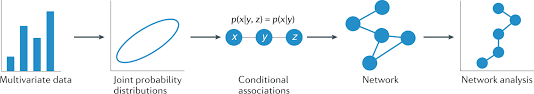
网络分析研究实体之间的关系,如个人、组织或文件。在多个层面上操作,它描述并推断单个实体、实体的子集和整个网络的关系属性。
statistics-lab™ 为您的留学生涯保驾护航 在代写网络分析Network Analysis方面已经树立了自己的口碑, 保证靠谱, 高质且原创的统计Statistics代写服务。我们的专家在代写网络分析Network Analysis代写方面经验极为丰富,各种代写网络分析Network Analysis相关的作业也就用不着说。
我们提供的网络分析Network Analysis及其相关学科的代写,服务范围广, 其中包括但不限于:
- Statistical Inference 统计推断
- Statistical Computing 统计计算
- Advanced Probability Theory 高等概率论
- Advanced Mathematical Statistics 高等数理统计学
- (Generalized) Linear Models 广义线性模型
- Statistical Machine Learning 统计机器学习
- Longitudinal Data Analysis 纵向数据分析
- Foundations of Data Science 数据科学基础

统计代写|网络分析代写Network Analysis代考|Organization of the book
We organize our book into the following chapters:
- Chapter 2: We introduce mathematical graph and properties. A graph is the basis of the entire graph theoretic modeling and analysis of biological networks. We even discuss the R scripting for handling graph data structures, briefly.
- Chapter 3: Various algorithms popularly studied in graph theory, such as graph traversal algorithms are discussed. In a biological network, power graph analysis is an important graph analysis method that we discuss with examples. Also, various node centrality measures are introduced and demonstrated with the help of $\mathrm{R}$ scripts.
- Chapter 4: Real-world networks follow certain special topological properties, which makes them different from the usual graph. Accordingly, they are classified into various network models. We use different models and their properties, and implement them using the R package.
- Chapter 5: The sources of three biological network repositories, which are publicly available databases, are discussed. The chapter starts with a basic introduction to popular and recently used database formats. It is a resourceful chapter for the biological network-related researches.
- Chapter 6: Gene expression networks have been introduced along with data generation sources for the expression networks. The overall discussion has been divided into two parts, in-silico network inference and post inference analysis. How gene network modules can be identified and how to rank important genes in an expression network has been discussed in the light of various algorithms. We even discuss various online and offline software tools to carry out gene expression network inference and analysis.
- Chapter 7: Protein and their physical interaction networks are vital to establishing true macromolecular connectivity in biological systems. How such interactions can be generated experimentally and predicted computationally has been highlighted. Recently, protein network alignment has gained importance in comparative network analysis for finding evolutionarily conserved proteins, which we include in this chapter. Few of the algorithms dealing with functional protein complex detection is discussed.
- Chapter 8: Finally, we introduce brain connectome networks with the input data sources and present trends in brain connectome network analysis.
统计代写|网络分析代写Network Analysis代考|Basic concepts
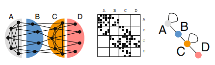
A graph [3] is a pictorial representation of a set of objects and their association with each other. The objects are popularly termed as nodes or vertices, and the associations are depicted using interconnections between pair of nodes, called edges. Mathematically, graphs are represented as a set of edges and vertices.
Definition 2.1.1 (Graph). A graph $\mathcal{G}$ is a pair of finite set of vertices and edges, $\mathcal{G}=(\mathcal{V}, \mathcal{E})$, such that $\mathcal{V}=\left{v_1, v_2, \cdots, v_n\right}$ and $\mathcal{E}=$ $\left{e_1, e_2, \cdots, e_m\right}$. An edge $e_k=\left(v_i, v_j\right)$ connects vertices $v_i$ and $v_j$
In the graph (Fig. 2.1), $\mathcal{V}={A, B, C, D, E, F}$ and $\mathcal{E}={(A, B)$, $(B, C),(C, D),(C, E),(E, E),(E, F),(E, D),(F, B)}$, where edges are an unordered pair of nodes having interconnections among them. Graph $\mathcal{G}$ is termed as undirected graph. The node $E$ is connected with itself through loop edge. A graph without my loop structure is called a simple graph.
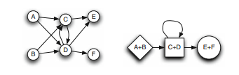
A graph with an ordered pair of nodes, where edges are associated with directions is called a directed graph or digraph.
Definition 2.1.2 (Directed graph). A directed graph $\mathcal{G}=(\mathcal{V}, \mathcal{E})$ is a set of vertices $\mathcal{V}$ and edges $\mathcal{E}$, such that, for any edge $\left(v_i, v_j\right)$ posses direction denoted by arrow. Unlike undirected graph, for any edge $v_i \rightarrow v_j$, the edge $\left(v_i, v_j\right) \neq\left(v_j, v_i\right)$. The node $v_i$ is called tail, and $v_j$ is referred to as head of the edge $v_i \rightarrow v_j$. For example, see Fig. 2.2.
Definition 2.1.3 (Path). A path is a sequence of distinct vertices that are connected by edges. In other words, given a set of vertices, $\left{v_1, v_2, \cdots, v_k\right} \in \mathcal{G}(\mathcal{V})$ is a path if for every pair of vertices $v_i$ and $v_{i+1}$ have an edge $\left(v_i, v_{i+1}\right) \in \mathcal{G}(\mathcal{E})$. However, in case of a directed graph, a directed path connects the sequence of vertices with the added restriction that all edges are oriented towards the same direction.
In a path, if sequences of vertices are not distinct, it is referred to as a walk.
Two nodes, $v_i$ and $v_j$, are reachable from each other if there is a path that exists between $v_i$ and $v_j$.
A path is called a closed path or cycle if two terminal nodes, $v_1$ and $v_k$, are connected in a path, i.e., $\left(v_k, v_1\right) \in \mathcal{G}(\mathcal{E})$.
网络分析代考
统计代写|网络分析代写Network Analysis代考|Organization of the book
我们将本书组织成以下章节:
- 第 2 章:我们介绍数学图和属性。图是整个图论建模和分析生物网络的基础。我们甚至简要讨论了用于处理图形数据结构的 R 脚本。
- 第三章:讨论图论中广泛研究的各种算法,如图遍历算法。在生物网络中,功率图分析是一种重要的图分析方法,我们将通过实例进行讨论。此外,还引入并演示了各种节点中心性度量R脚本。
- 第 4 章:现实世界的网络遵循某些特殊的拓扑属性,这使得它们不同于通常的图。因此,它们被分类为各种网络模型。我们使用不同的模型及其属性,并使用 R 包实现它们。
- 第 5 章:讨论了三个生物网络存储库的来源,它们是公开可用的数据库。本章从对流行和最近使用的数据库格式的基本介绍开始。这是生物网络相关研究的丰富篇章。
- 第 6 章:介绍了基因表达网络以及表达网络的数据生成源。整体讨论分为两个部分,in-silico network inference 和 post inference analysis。已经根据各种算法讨论了如何识别基因网络模块以及如何对表达网络中的重要基因进行排序。我们甚至讨论了各种在线和离线软件工具来进行基因表达网络推断和分析。
- 第 7 章:蛋白质及其物理相互作用网络对于在生物系统中建立真正的大分子连接至关重要。已经强调了如何通过实验产生这种相互作用并通过计算进行预测。最近,蛋白质网络比对在比较网络分析中变得越来越重要,以寻找进化上保守的蛋白质,我们将在本章中介绍。很少讨论处理功能性蛋白质复合物检测的算法。
- 第 8 章:最后,我们介绍了具有输入数据源的脑连接组网络,并介绍了脑连接组网络分析的趋势。
统计代写|网络分析代写Network Analysis代考|Basic concepts
图 [3] 是一组对象及其相互关联的图形表示。对象通常被称为节点或顶点,并且使用称为边的节点对之间的互连来 描述关联。在数学上,图被表示为一组边和顶点。
定义 2.1.1 (图表)。图表 $\mathcal{G}$ 是一对有限的顶点和边集, $\mathcal{G}=(\mathcal{V}, \mathcal{E})$, 这样 点 $v_i$ 和 $v_j$
在图表中 (图 2.1), $\mathcal{V}=A, B, C, D, E, F$ 和
$\mathcal{E}=(A, B) \$ \$(B, C),(C, D),(C, E),(E, E),(E, F),(E, D),(F, B)$ ,其中边是一对无序的节点,它们 之间有互连。图形 $\mathcal{G}$ 称为无向图。节点 $E$ 通过环边与自身相连。没有我的循环结构的图称为简单图。
具有有序节点对的图,其中边与方向相关联,称为有向图或有向图。
定义 2.1.2 (有向图) 。有向图 $\mathcal{G}=(\mathcal{V}, \mathcal{E})$ 是一组顶点 $\mathcal{V}$ 和边缘 $\mathcal{E}$ ,这样,对于任何边缘 $\left(v_i, v_j\right)$ 具有箭头所指的 方向。与无向图不同,对于任何边 $v_i \rightarrow v_j$ ,边缘 $\left(v_i, v_j\right) \neq\left(v_j, v_i\right)$. 节点 $v_i$ 称为尾巴,并且 $v_j$ 被称为边缘的头 部 $v_i \rightarrow v_j$. 例如,见图 2.2。
定义 2.1.3 (路径) 。路径是由边连接的一系列不同顶点。换句话说,给定一组顶点,
$\left(v_i, v_{i+1}\right) \in \mathcal{G}(\mathcal{E})$. 但是,在有向图的情况下,有向路径将顶点序列连接起来,并增加了所有边都朝向同一方向 的限制。
在路径中,如果顶点序列不是不同的,则称为游走。
两个节点, $v_i$ 和 $v_j$ ,如果存在路径,则彼此可达 $v_i$ 和 $v_j$.
如果有两个终端节点,则路径称为闭合路径或循环, $v_1$ 和 $v_k$ ,连接在一条路径上,即 $\left(v_k, v_1\right) \in \mathcal{G}(\mathcal{E})$.

统计代写请认准statistics-lab™. statistics-lab™为您的留学生涯保驾护航。
金融工程代写
金融工程是使用数学技术来解决金融问题。金融工程使用计算机科学、统计学、经济学和应用数学领域的工具和知识来解决当前的金融问题,以及设计新的和创新的金融产品。
非参数统计代写
非参数统计指的是一种统计方法,其中不假设数据来自于由少数参数决定的规定模型;这种模型的例子包括正态分布模型和线性回归模型。
广义线性模型代考
广义线性模型(GLM)归属统计学领域,是一种应用灵活的线性回归模型。该模型允许因变量的偏差分布有除了正态分布之外的其它分布。
术语 广义线性模型(GLM)通常是指给定连续和/或分类预测因素的连续响应变量的常规线性回归模型。它包括多元线性回归,以及方差分析和方差分析(仅含固定效应)。
有限元方法代写
有限元方法(FEM)是一种流行的方法,用于数值解决工程和数学建模中出现的微分方程。典型的问题领域包括结构分析、传热、流体流动、质量运输和电磁势等传统领域。
有限元是一种通用的数值方法,用于解决两个或三个空间变量的偏微分方程(即一些边界值问题)。为了解决一个问题,有限元将一个大系统细分为更小、更简单的部分,称为有限元。这是通过在空间维度上的特定空间离散化来实现的,它是通过构建对象的网格来实现的:用于求解的数值域,它有有限数量的点。边界值问题的有限元方法表述最终导致一个代数方程组。该方法在域上对未知函数进行逼近。[1] 然后将模拟这些有限元的简单方程组合成一个更大的方程系统,以模拟整个问题。然后,有限元通过变化微积分使相关的误差函数最小化来逼近一个解决方案。
tatistics-lab作为专业的留学生服务机构,多年来已为美国、英国、加拿大、澳洲等留学热门地的学生提供专业的学术服务,包括但不限于Essay代写,Assignment代写,Dissertation代写,Report代写,小组作业代写,Proposal代写,Paper代写,Presentation代写,计算机作业代写,论文修改和润色,网课代做,exam代考等等。写作范围涵盖高中,本科,研究生等海外留学全阶段,辐射金融,经济学,会计学,审计学,管理学等全球99%专业科目。写作团队既有专业英语母语作者,也有海外名校硕博留学生,每位写作老师都拥有过硬的语言能力,专业的学科背景和学术写作经验。我们承诺100%原创,100%专业,100%准时,100%满意。
随机分析代写
随机微积分是数学的一个分支,对随机过程进行操作。它允许为随机过程的积分定义一个关于随机过程的一致的积分理论。这个领域是由日本数学家伊藤清在第二次世界大战期间创建并开始的。
时间序列分析代写
随机过程,是依赖于参数的一组随机变量的全体,参数通常是时间。 随机变量是随机现象的数量表现,其时间序列是一组按照时间发生先后顺序进行排列的数据点序列。通常一组时间序列的时间间隔为一恒定值(如1秒,5分钟,12小时,7天,1年),因此时间序列可以作为离散时间数据进行分析处理。研究时间序列数据的意义在于现实中,往往需要研究某个事物其随时间发展变化的规律。这就需要通过研究该事物过去发展的历史记录,以得到其自身发展的规律。
回归分析代写
多元回归分析渐进(Multiple Regression Analysis Asymptotics)属于计量经济学领域,主要是一种数学上的统计分析方法,可以分析复杂情况下各影响因素的数学关系,在自然科学、社会和经济学等多个领域内应用广泛。
MATLAB代写
MATLAB 是一种用于技术计算的高性能语言。它将计算、可视化和编程集成在一个易于使用的环境中,其中问题和解决方案以熟悉的数学符号表示。典型用途包括:数学和计算算法开发建模、仿真和原型制作数据分析、探索和可视化科学和工程图形应用程序开发,包括图形用户界面构建MATLAB 是一个交互式系统,其基本数据元素是一个不需要维度的数组。这使您可以解决许多技术计算问题,尤其是那些具有矩阵和向量公式的问题,而只需用 C 或 Fortran 等标量非交互式语言编写程序所需的时间的一小部分。MATLAB 名称代表矩阵实验室。MATLAB 最初的编写目的是提供对由 LINPACK 和 EISPACK 项目开发的矩阵软件的轻松访问,这两个项目共同代表了矩阵计算软件的最新技术。MATLAB 经过多年的发展,得到了许多用户的投入。在大学环境中,它是数学、工程和科学入门和高级课程的标准教学工具。在工业领域,MATLAB 是高效研究、开发和分析的首选工具。MATLAB 具有一系列称为工具箱的特定于应用程序的解决方案。对于大多数 MATLAB 用户来说非常重要,工具箱允许您学习和应用专业技术。工具箱是 MATLAB 函数(M 文件)的综合集合,可扩展 MATLAB 环境以解决特定类别的问题。可用工具箱的领域包括信号处理、控制系统、神经网络、模糊逻辑、小波、仿真等。