如果你也在 怎样代写微观经济学Microeconomics这个学科遇到相关的难题，请随时右上角联系我们的24/7代写客服。

微观经济学是研究稀缺性及其对资源的使用、商品和服务的生产、生产和福利的长期增长的影响，以及对社会至关重要的其他大量复杂问题的研究。

statistics-lab™ 为您的留学生涯保驾护航 在代写微观经济学Microeconomics方面已经树立了自己的口碑, 保证靠谱, 高质且原创的统计Statistics代写服务。我们的专家在代写微观经济学Microeconomics代写方面经验极为丰富，各种代写微观经济学Microeconomics相关的作业也就用不着说。

我们提供的微观经济学Microeconomics及其相关学科的代写，服务范围广, 其中包括但不限于:

• Statistical Inference 统计推断
• Statistical Computing 统计计算
• Advanced Probability Theory 高等概率论
• Advanced Mathematical Statistics 高等数理统计学
• (Generalized) Linear Models 广义线性模型
• Statistical Machine Learning 统计机器学习
• Longitudinal Data Analysis 纵向数据分析
• Foundations of Data Science 数据科学基础

经济代写|微观经济学代写Microeconomics代考|Oligopoly

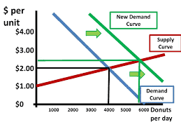
In an oligopoly a few producers satisfy the demand of many consumers. Different to perfectly competitive markets or monopolies, these producers pay attention to the behavior of the other oligopolists. As such, strategies play an important role in oligopolies and game theory is the foremost tool to study the behavior. Quantity and price in an oligopoly will be somewhere between monopoly and perfect competition.

In many cases, economists study oligopolies with the help of game theory. Game theory analyzes strategic interactions between rational decision-makers with the help of mathematical models. Founding fathers of game theory were von Neumann and Morgenstern (1944). Nash (1951) defined an equilibrium solution to a noncooperative game which later became known as Nash equilibrium. This is a situation where no player can change his strategy without becoming worse off if all other players keep their strategy.

A simple form of an oligopoly is a duopoly, the competition between two producers. Cournot (1838) developed a solution to the problem implying that producer A chooses his output by assuming a fixed output from producer $B$ (and vice versa) without further adjustments. This provides a stable equilibrium at a level below monopoly price and above monopoly quantity. The behavior of the two producers can be described as a simultaneous competition for quantities.

In the Stackelberg model (1934), producer A would anticipate the move of B and factor this outcome into his strategy in order to increase his own profit (and decrease the profit of B). The total profit of both producers will be smaller than the profits in the Cournot model and the monopoly but higher than in perfectly competitive markets. We are looking in difference to the Cournot model at a sequential competition for quantities.

The market outcomes are often suboptimal from the point of view of the oligopolists; the solutions do not reach an equilibrium. They might in such cases be tempted to collude by fixing prices. While this happens in real life and also in construction, it is illegal.

Oligopolies make use of advertising. These activities increase the costs of the producers and they are called transaction costs. Oligopolists and others facing such transaction costs will have to consider these in addition to the rule $M R=M C$. They create a gap between buying and selling price reducing the market quantity (Hirshleifer and Hirshleifer 1998, p. 410).

Specific market conditions need to be looked at to find a solution for an oligopoly since there are otherwise infinite possibilities of strategic behaviors. It seems to be advisable to look at the construction market in detail before advancing the theory of oligopolies (Chapter 14). We will find that oligopolies play a negligible role in construction.

经济代写|微观经济学代写Microeconomics代考|Factor Supply of Households

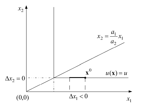
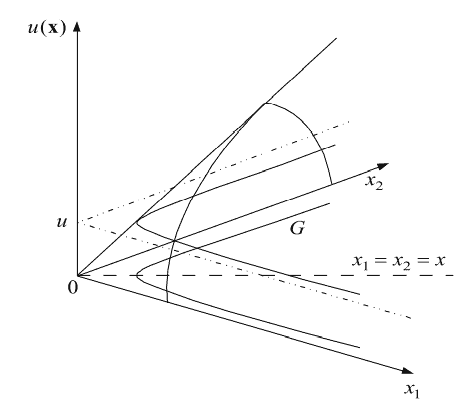
Households need money in order to be able to purchase necessary and luxury goods. The only chance for the majority is to offer their labor in the labor market and to earn a wage. To this end, individuals and households make decisions how they use their time. Time is a limited resource as the day has invariably 24 hours. An individual can choose how much time to spend working $(W)$ and economists call the remaining part of the day leisure $(L)$ whether it is used for cleaning, cooking, learning, or relaxing. The less an individual works, the less money he has for consumption and the more time for other activities. Instead of a budget constraint, the individual faces now a time constraint. Instead of choosing between a number of different goods, we are now looking at the time preferences of the individual. As before, constraints and preferences determine the decision of the individual in the neoclassical model (Figure 7.2).

A person can theoretically work 24 hours, and this provides the $y$-intercept for the time constraint; it also can work 0 hours and spend all day on leisure ( $x$-intercept). This way we can construct the time constraint in Figure 7.2. The explanations for the construction of indifference lines and utility maximization in Section 3.3 on consumer behavior are also valid for time preferences and maximizing decisions on the use of time.

It should be clear that most people are not free to decide how many hours to work, but looking at a total work life, there certainly is some flexibility for many. Changes in preferences lead to different choices. In some Western countries, young engineers today value leisure more than the generations before them. In other words, they prefer spending time with family and friends. Figure 7.3 shows the different preferences and outcomes.

The daily income $(y)$ is the product of work hours $\left(h_{\mathrm{W}}\right)$ and wage, and if we consider theoretically 24 hours as the maximum available time, then the choice of leisure hours $\left(h_{\mathrm{L}}\right)$ influences this income:
$$
y=w \cdot h_{\mathrm{W}}=w\left(24-h_{\mathrm{L}}\right)
$$
Differentiating Eq. (7.1) for $h_{\mathrm{L}}$ gives:
$$
d y / d h_L=-w
$$
Thus, the income-leisure combination has a slope of $-w$. An increase in income due to a higher wage can shift the choice toward more leisure time (Figure 7.4). This depends, of course, on the shape of the preference curves, but it is one possible outcome.

微观经济学代考

经济代写|微观经济学代写Microeconomics代考|Oligopoly

在寡头垄断中，少数生产者满足许多消费者的需求。与完全竞争市场或垄断不同，这些生产者关注其他寡头的行为。因此，策略在寡头垄断中起着重要作用，博弈论是研究行为的最重要工具。寡头垄断中的数量和价格介于垄断和完全竞争之间。

在许多情况下，经济学家在博弈论的帮助下研究寡头垄断。博弈论借助数学模型分析理性决策者之间的战略互动。博弈论的奠基人是冯·诺依曼和摩根斯坦（1944 年）。Nash (1951) 定义了非合作博弈的均衡解，后来被称为纳什均衡。在这种情况下，如果所有其他玩家都保持他们的策略，则没有玩家可以在不变得更糟的情况下改变他的策略。

寡头垄断的一种简单形式是双头垄断，即两个生产者之间的竞争。古诺 (Cournot, 1838) 提出了一个问题的解决方案，即生产者 A 通过假设生产者的固定输出来选择他的输出乙（反之亦然）无需进一步调整。这在低于垄断价格和高于垄断数量的水平上提供了稳定的均衡。两家生产商的行为可以描述为同时进行数量竞争。

在 Stackelberg 模型（1934 年）中，生产商 A 会预期 B 的移动并将这一结果纳入其战略，以增加自己的利润（并减少 B 的利润）。两个生产者的总利润将小于古诺模型和垄断中的利润，但高于完全竞争市场中的利润。我们正在寻找与古诺模型在数量顺序竞争中的区别。

从寡头垄断者的角度来看，市场结果往往是次优的；解决方案没有达到平衡。在这种情况下，他们可能会试图通过固定价格来串通一气。虽然这种情况发生在现实生活和建筑中，但它是非法的。

寡头垄断利用广告。这些活动增加了生产者的成本，它们被称为交易成本。除了规则之外，寡头垄断者和其他面临此类交易成本的人将不得不考虑这些米R=米C. 他们在买卖价格之间制造差距，减少市场数量（Hirshleifer 和 Hirshleifer 1998，第 410 页）。

需要查看特定的市场条件以找到寡头垄断的解决方案，因为否则存在无限的战略行为可能性。在推进寡头垄断理论（第 14 章）之前，详细研究建筑市场似乎是明智的。我们会发现寡头垄断在建设中的作用微乎其微。

经济代写|微观经济学代写Microeconomics代考|Factor Supply of Households

家庭需要钱才能购买必需品和奢侈品。大多数人的唯一机会是在劳动力市场上提供劳动力并赚取工资。为 此，个人和家庭决定如何使用他们的时间。时间是有限的资源，因为一天总是 24 小时。个人可以选择花多 少时间工作 $(W)$ 经济学家称一天的剩余时间为休闲 $(L)$ 无论是用于清洁、亨饪、学习还是放松。一个人的 工作越少，他用于消费的钱就越少，用于其他活动的时间就越多。个人现在面临的不是预算限制，而是时 间限制。我们现在不是在许多不同的商品之间进行选择，而是关注个人的时间偏好。和以前一样，约束和 偏好决定了新古典模型中个人的决策 (图 7.2)。
一个人理论上可以24小时工作，这提供了 $y$-拦截时间限制；它还可以工作0小时，整天休闲 ( $x$-截距) 。这 样我们就可以构建图 7.2 中的时间约束。 3.3 节关于消费者行为的无差异线构造和效用最大化的解释也适用 于时间偏好和时间使用最大化决策。
应该清楚的是，大多数人不能自由决定工作多少小时，但从总的工作时间来看，对许多人来说肯定有一定 的灵活性。偏好的变化导致不同的选择。在一些西方国家，今天的年轻工程师比他们的前几代人更看重休 闲。换句话说，他们更喜欢与家人和朋友共度时光。图 7.3 显示了不同的偏好和结果。
每天的收入 $(y)$ 是工作时间的产物 $\left(h_{\mathrm{W}}\right)$ 和工资，如果我们将理论上的 24 小时视为最大可用时间，那么休 闲时间的选择 $\left(h_{\mathrm{L}}\right)$ 影响收入:
$$
y=w \cdot h_{\mathrm{W}}=w\left(24-h_{\mathrm{L}}\right)
$$
微分方程 (7.1) 对于 $h_{\mathrm{L}}$ 给出:
$$
d y / d h_L=-w
$$
因此，收入-休闲组合的斜率为 $-w$. 由于更高的工资而增加的收入可以将选择转向更多的闲暇时间 (图 7.4）。当然，这取决于偏好曲线的形状，但这是一种可能的结果。

统计代写请认准statistics-lab™. statistics-lab™为您的留学生涯保驾护航。

金融工程代写

金融工程是使用数学技术来解决金融问题。金融工程使用计算机科学、统计学、经济学和应用数学领域的工具和知识来解决当前的金融问题，以及设计新的和创新的金融产品。

非参数统计代写

非参数统计指的是一种统计方法，其中不假设数据来自于由少数参数决定的规定模型；这种模型的例子包括正态分布模型和线性回归模型。

广义线性模型代考

广义线性模型（GLM）归属统计学领域，是一种应用灵活的线性回归模型。该模型允许因变量的偏差分布有除了正态分布之外的其它分布。

术语 广义线性模型（GLM）通常是指给定连续和/或分类预测因素的连续响应变量的常规线性回归模型。它包括多元线性回归，以及方差分析和方差分析（仅含固定效应）。

有限元方法代写

有限元方法（FEM）是一种流行的方法，用于数值解决工程和数学建模中出现的微分方程。典型的问题领域包括结构分析、传热、流体流动、质量运输和电磁势等传统领域。

有限元是一种通用的数值方法，用于解决两个或三个空间变量的偏微分方程（即一些边界值问题）。为了解决一个问题，有限元将一个大系统细分为更小、更简单的部分，称为有限元。这是通过在空间维度上的特定空间离散化来实现的，它是通过构建对象的网格来实现的：用于求解的数值域，它有有限数量的点。边界值问题的有限元方法表述最终导致一个代数方程组。该方法在域上对未知函数进行逼近。[1] 然后将模拟这些有限元的简单方程组合成一个更大的方程系统，以模拟整个问题。然后，有限元通过变化微积分使相关的误差函数最小化来逼近一个解决方案。

tatistics-lab作为专业的留学生服务机构，多年来已为美国、英国、加拿大、澳洲等留学热门地的学生提供专业的学术服务，包括但不限于Essay代写，Assignment代写，Dissertation代写，Report代写，小组作业代写，Proposal代写，Paper代写，Presentation代写，计算机作业代写，论文修改和润色，网课代做，exam代考等等。写作范围涵盖高中，本科，研究生等海外留学全阶段，辐射金融，经济学，会计学，审计学，管理学等全球99%专业科目。写作团队既有专业英语母语作者，也有海外名校硕博留学生，每位写作老师都拥有过硬的语言能力，专业的学科背景和学术写作经验。我们承诺100%原创，100%专业，100%准时，100%满意。

随机分析代写

随机微积分是数学的一个分支，对随机过程进行操作。它允许为随机过程的积分定义一个关于随机过程的一致的积分理论。这个领域是由日本数学家伊藤清在第二次世界大战期间创建并开始的。

时间序列分析代写

随机过程，是依赖于参数的一组随机变量的全体，参数通常是时间。 随机变量是随机现象的数量表现，其时间序列是一组按照时间发生先后顺序进行排列的数据点序列。通常一组时间序列的时间间隔为一恒定值（如1秒，5分钟，12小时，7天，1年），因此时间序列可以作为离散时间数据进行分析处理。研究时间序列数据的意义在于现实中，往往需要研究某个事物其随时间发展变化的规律。这就需要通过研究该事物过去发展的历史记录，以得到其自身发展的规律。

回归分析代写

多元回归分析渐进（Multiple Regression Analysis Asymptotics）属于计量经济学领域，主要是一种数学上的统计分析方法，可以分析复杂情况下各影响因素的数学关系，在自然科学、社会和经济学等多个领域内应用广泛。

MATLAB代写

MATLAB 是一种用于技术计算的高性能语言。它将计算、可视化和编程集成在一个易于使用的环境中，其中问题和解决方案以熟悉的数学符号表示。典型用途包括：数学和计算算法开发建模、仿真和原型制作数据分析、探索和可视化科学和工程图形应用程序开发，包括图形用户界面构建MATLAB 是一个交互式系统，其基本数据元素是一个不需要维度的数组。这使您可以解决许多技术计算问题，尤其是那些具有矩阵和向量公式的问题，而只需用 C 或 Fortran 等标量非交互式语言编写程序所需的时间的一小部分。MATLAB 名称代表矩阵实验室。MATLAB 最初的编写目的是提供对由 LINPACK 和 EISPACK 项目开发的矩阵软件的轻松访问，这两个项目共同代表了矩阵计算软件的最新技术。MATLAB 经过多年的发展，得到了许多用户的投入。在大学环境中，它是数学、工程和科学入门和高级课程的标准教学工具。在工业领域，MATLAB 是高效研究、开发和分析的首选工具。MATLAB 具有一系列称为工具箱的特定于应用程序的解决方案。对于大多数 MATLAB 用户来说非常重要，工具箱允许您学习和应用专业技术。工具箱是 MATLAB 函数（M 文件）的综合集合，可扩展 MATLAB 环境以解决特定类别的问题。可用工具箱的领域包括信号处理、控制系统、神经网络、模糊逻辑、小波、仿真等。

R语言代写	问卷设计与分析代写
PYTHON代写	回归分析与线性模型代写
MATLAB代写	方差分析与试验设计代写
STATA代写	机器学习/统计学习代写
SPSS代写	计量经济学代写
EVIEWS代写	时间序列分析代写
EXCEL代写	深度学习代写
SQL代写	各种数据建模与可视化代写

如果你也在 怎样代写微观经济学Microeconomics这个学科遇到相关的难题，请随时右上角联系我们的24/7代写客服。

微观经济学是研究稀缺性及其对资源的使用、商品和服务的生产、生产和福利的长期增长的影响，以及对社会至关重要的其他大量复杂问题的研究。

statistics-lab™ 为您的留学生涯保驾护航 在代写微观经济学Microeconomics方面已经树立了自己的口碑, 保证靠谱, 高质且原创的统计Statistics代写服务。我们的专家在代写微观经济学Microeconomics代写方面经验极为丰富，各种代写微观经济学Microeconomics相关的作业也就用不着说。

我们提供的微观经济学Microeconomics及其相关学科的代写，服务范围广, 其中包括但不限于:

• Statistical Inference 统计推断
• Statistical Computing 统计计算
• Advanced Probability Theory 高等概率论
• Advanced Mathematical Statistics 高等数理统计学
• (Generalized) Linear Models 广义线性模型
• Statistical Machine Learning 统计机器学习
• Longitudinal Data Analysis 纵向数据分析
• Foundations of Data Science 数据科学基础

经济代写|微观经济学代写Microeconomics代考|Monopolistic Competition

Monopolistic competition is the most prevalent market configuration besides heterogenous oligopolies. Under these conditions, producers offer differentiated products – and not homogenous goods – that serve the same purpose such as T-shirts, and consumers have preferences for certain products. This allows some space for producers to set prices. They are no longer price-takers but they also do not have the freedom of normal monopolists. Their market power is more limited. Producers can differentiate products mainly by style, location, or quality. The more a producer is able to differentiate the products, the stronger the market power. Each producer provides only a relatively small quantity of goods to the market so that its actions have no impact on other producers. Thus, if a producer raises the price of a product, it will lose some customers but not all, as under the conditions of perfect competition.

However, the producer is threatened by new firms who can enter the market and attack the differentiated product. The possibility of free market entry reduces profits to zero in the long run. This result is the same as for perfect competition, but other results are different, as we will see.

The excess capacity theorem assumes a classical production function and corresponding cost curves as well as the same costs for all producers. Figure 6.4 illustrates the situation. The demand curve is again downward sloping and the slope of marginal revenue curve is twice as much as the demand curve. The marginal cost curve (supply) is upward sloping. As there are some fixed costs, total average costs are U-shaped. Profit maximizing is the quantity $q^{m c}$ where marginal costs equal marginal revenue and the corresponding price is $p^{m c}$. If the average total cost curve lies below the demand curve, the monopolistic competitor generates a profit.

The strength of consumer preferences for a differentiated product is represented in the elasticity of the demand curve. The stronger the preference, the more inelastic will be the demand curve (Figure 6.4, right).

In the short run, the monopolistic competitor will act as monopolist dealing with cost curves from the classical production function (Figure 6.5, left). With market entry, the demand and marginal revenue curves will swivel around point $\mathrm{A}$ and become more elastic. The $y$-intercept moves from B to B’ (Figure 6.5, right). The price is lowered and the offered quantity is also reduced. This reduces the monopolistic profit.

经济代写|微观经济学代写Microeconomics代考|Monopsony

Monopsonies play a role in the construction sector. The government or government agencies act sometimes as the sole buyer in a market. In many countries, it is the exclusive right and duty of the government to provide public roads. As these are by far the majority of all roads, the government acts as monopsonist. The same often holds true for railroads. Thus, monopsonies are of interest. The owner in construction will not be a consumer (one-family home) but an investor and will thus act on factor markets (Chapter 7).

A typical case in the microeconomic literature to explain monopsonies is one employer looking for labor (Nicholson and Snyder 2014). This could be a large firm in a small town. If one producer is the asking for the by-far-largest supply of labor from a relatively large number of workers, then that producer holds a monopsony position. This is the inverse of a monopoly.

If we call $p \cdot \partial q / \partial L$ the marginal value product of labor $\left(M V P_L\right)$, then we know that this must equal the wage if the producer is maximizing the profit in perfectly competitive markets. If we assume diminishing marginal labor productivity, then the $\mathrm{MVP}_{\mathrm{L}}$ curve is downward sloping (Figure 6.8).

The labor supply curve is sloping upward because the monopsonist is not facing a negligible quantity of labor but the majority of the labor supply in a regional market. If the monpsonist hires one more worker, this worker is only willing to accept above market price. If all workers receive the same wage, this means that adding one more worker increases total cost by the pay for the worker and the increase for all other workers. The cost of hiring one more worker is always higher than the market price. Consequently, the marginal expense curve will always be above the labor supply curve.

A producer in a perfectly competitive market will hire more labor until the additional marginal costs $M E_{\mathrm{L}}$ are equal to the additional marginal revenue $M R_{\mathrm{L}}$. If the costs were higher, then the producer would lose money; if the costs were lower, it would forgo the opportunity to increase its profit:
$$
M E_{\mathrm{L}}=M R_{\mathrm{L}}
$$
The monopsonist will add labor until the marginal revenue of labor equals the MVP:
$$
M R_{\mathrm{L}}=M V P_{\mathrm{L}}
$$
If the producer were a price taker, then the intersection of the downward-sloping demand curve and the upward-sloping supply curve would provide the market equilibrium. This is marked as $L_{\mathrm{C}}$ and $w_{\mathrm{C}}$ in Figure 6.9. Since a monopsonist is not a price taker, the marginal revenue curve (expense curve) lies above the supply curve and this determines actual labor demand by $M R_{\mathrm{L}}=M V P_{\mathrm{L}}$. Thus, the monopsonist demands less labor $\left(L_{\mathrm{M}}\right)$ at a lower wage $\left(w_M\right)$ by using its market power.

The more inelastic the labor supply curve is, the lower will the wage be. To see this effect, you just have to rotate the supply curve more upward around the point $L_{\mathrm{C}} / w_{\mathrm{C}}$.

微观经济学代考

经济代写|微观经济学代写Microeconomics代考|Monopolistic Competition

垄断竞争是除异质寡头垄断之外最普遍的市场配置。在这些条件下，生产商提供差异化​​产品——而不是同质产品——服务于相同的目的，例如 T 恤，消费者对某些产品有偏好。这为生产商设定价格提供了一些空间。他们不再是价格接受者，但他们也没有正常垄断者的自由。他们的市场力量更加有限。生产商可以主要通过风格、位置或质量来区分产品。生产者越能够区分产品，市场力量就越强。每个生产者只向市场提供相对少量的商品，因此其行为不会影响其他生产者。因此，如果生产者提高产品价格，

然而，生产者受到可以进入市场并攻击差异化产品的新公司的威胁。从长远来看，自由市场进入的可能性会使利润减少到零。这个结果与完全竞争相同，但其他结果不同，我们将看到。

产能过剩定理假设一个经典的生产函数和相应的成本曲线以及所有生产者的相同成本。图 6.4 说明了这种情况。需求曲线再次向下倾斜，边际收益曲线的斜率是需求曲线的两倍。边际成本曲线（供给）向上倾斜。由于有一些固定成本，总平均成本呈 U 形。利润最大化是数量q米C其中边际成本等于边际收益，相应的价格是p米C. 如果平均总成本曲线位于需求曲线下方，则垄断竞争者产生利润。

消费者对差异化产品的偏好强度体现在需求曲线的弹性上。偏好越强，需求曲线就越缺乏弹性（图 6.4，右）。

在短期内，垄断竞争者将作为垄断者处理经典生产函数的成本曲线（图 6.5，左）。随着市场进入，需求和边际收益曲线将围绕点旋转A并变得更有弹性。这和-拦截从 B 移动到 B’（图 6.5，右）。价格降低，报价数量也减少。这减少了垄断利润。

经济代写|微观经济学代写Microeconomics代考|Monopsony

垄断在建筑行业发挥作用。政府或政府机构有时充当市场上的唯一买家。在许多国家，提供公共道路是政 府的专有权利和义务。由于这些是迄今为止所有道路中的大多数，因此政府充当垄断者。铁路也是如此。 因此，芢断是令人感兴趣的。建筑业主将不是消费者（单户住宅），而是投资者，因此将在要素市场上行 动（第 7 章)。
微观经济学文献中解释垄断的典型案例是一个雇主在寻找劳动力 (Nicholson 和 Snyder 2014)。这可能 是一个小镇上的大公司。如果一个生产者要求相对大量的工人提供迄今为止最大的劳动力供应，那么该生 产者就处于垄断地位。这与䞣断相反。
如果我们打电话 $p \cdot \partial q / \partial L$ 劳动的边际价值产品 $\left(M V P_L\right)$ ，那么我们就知道，如果生产者在完全竞争市场 上实现利润最大化，那么这一定等于工资。如果我们假设边际劳动生产率递减，那么 $M_V \mathrm{PP}{\mathrm{L}}$ 曲线向下倾斜 (图 6.8)。 劳动力供给曲线向上倾斜，因为龿断者面对的不是微不足道的劳动力，而是区域市场中的大部分劳动力供 给。如果 monpsonist 再雇用一名工人，这名工人只愿意接受高于市场价格的价格。如果所有工人获得相 司的工资，这意味着增加一名工人会增加总成本，增加的部分是该工人的工资和所有其他工人的增加。多 蒮一名工人的成本总是高于市场价格。因此，边际费用曲线将始终高于劳动力供给曲线。 完全竞争市场中的生产者将雇佣更多的劳动力，直到额外的边际成本 $M E{\mathrm{L}}$ 等于额外的边际收益 $M R_{\mathrm{L}}$. 如 果成本更高，那么生产商就会赔钱；如果成本较低，它将放弃增加利润的机会：
$$
M E_{\mathrm{L}}=M R_{\mathrm{L}}
$$
垄断者将增加劳动力，直到劳动力的边际收益等于 MVP：
$$
M R_{\mathrm{L}}=M V P_{\mathrm{L}}
$$
如果生产者是价格接受者，那么向下倾斜的需求曲线和向上倾斜的供给曲线的交点将提供市场均衡。这被 标记为 $L_{\mathrm{C}}$ 和 $w_{\mathrm{C}}$ 在图 6.9 中。由于垄断者不是价格接受者，边际收益曲线 (费用曲线) 位于供给曲线之 上，这决定了实际劳动力需求 $M R_{\mathrm{L}}=M V P_{\mathrm{L}}$. 因此，垄断者需要更少的劳动力 $\left(L_{\mathrm{M}}\right)$ 以较低的工资 $\left(w_M\right)$ 通过利用其市场力量。
劳动力供给曲线越缺乏弹性，工资就越低。要看到这种效果，您只需将供应曲线围绕该点向上旋转
$$
L_{\mathrm{C}} / w_{\mathrm{C}}
$$

统计代写请认准statistics-lab™. statistics-lab™为您的留学生涯保驾护航。

金融工程代写

金融工程是使用数学技术来解决金融问题。金融工程使用计算机科学、统计学、经济学和应用数学领域的工具和知识来解决当前的金融问题，以及设计新的和创新的金融产品。

非参数统计代写

非参数统计指的是一种统计方法，其中不假设数据来自于由少数参数决定的规定模型；这种模型的例子包括正态分布模型和线性回归模型。

广义线性模型代考

广义线性模型（GLM）归属统计学领域，是一种应用灵活的线性回归模型。该模型允许因变量的偏差分布有除了正态分布之外的其它分布。

术语 广义线性模型（GLM）通常是指给定连续和/或分类预测因素的连续响应变量的常规线性回归模型。它包括多元线性回归，以及方差分析和方差分析（仅含固定效应）。

有限元方法代写

有限元方法（FEM）是一种流行的方法，用于数值解决工程和数学建模中出现的微分方程。典型的问题领域包括结构分析、传热、流体流动、质量运输和电磁势等传统领域。

有限元是一种通用的数值方法，用于解决两个或三个空间变量的偏微分方程（即一些边界值问题）。为了解决一个问题，有限元将一个大系统细分为更小、更简单的部分，称为有限元。这是通过在空间维度上的特定空间离散化来实现的，它是通过构建对象的网格来实现的：用于求解的数值域，它有有限数量的点。边界值问题的有限元方法表述最终导致一个代数方程组。该方法在域上对未知函数进行逼近。[1] 然后将模拟这些有限元的简单方程组合成一个更大的方程系统，以模拟整个问题。然后，有限元通过变化微积分使相关的误差函数最小化来逼近一个解决方案。

tatistics-lab作为专业的留学生服务机构，多年来已为美国、英国、加拿大、澳洲等留学热门地的学生提供专业的学术服务，包括但不限于Essay代写，Assignment代写，Dissertation代写，Report代写，小组作业代写，Proposal代写，Paper代写，Presentation代写，计算机作业代写，论文修改和润色，网课代做，exam代考等等。写作范围涵盖高中，本科，研究生等海外留学全阶段，辐射金融，经济学，会计学，审计学，管理学等全球99%专业科目。写作团队既有专业英语母语作者，也有海外名校硕博留学生，每位写作老师都拥有过硬的语言能力，专业的学科背景和学术写作经验。我们承诺100%原创，100%专业，100%准时，100%满意。

随机分析代写

随机微积分是数学的一个分支，对随机过程进行操作。它允许为随机过程的积分定义一个关于随机过程的一致的积分理论。这个领域是由日本数学家伊藤清在第二次世界大战期间创建并开始的。

时间序列分析代写

随机过程，是依赖于参数的一组随机变量的全体，参数通常是时间。 随机变量是随机现象的数量表现，其时间序列是一组按照时间发生先后顺序进行排列的数据点序列。通常一组时间序列的时间间隔为一恒定值（如1秒，5分钟，12小时，7天，1年），因此时间序列可以作为离散时间数据进行分析处理。研究时间序列数据的意义在于现实中，往往需要研究某个事物其随时间发展变化的规律。这就需要通过研究该事物过去发展的历史记录，以得到其自身发展的规律。

回归分析代写

多元回归分析渐进（Multiple Regression Analysis Asymptotics）属于计量经济学领域，主要是一种数学上的统计分析方法，可以分析复杂情况下各影响因素的数学关系，在自然科学、社会和经济学等多个领域内应用广泛。

MATLAB代写

MATLAB 是一种用于技术计算的高性能语言。它将计算、可视化和编程集成在一个易于使用的环境中，其中问题和解决方案以熟悉的数学符号表示。典型用途包括：数学和计算算法开发建模、仿真和原型制作数据分析、探索和可视化科学和工程图形应用程序开发，包括图形用户界面构建MATLAB 是一个交互式系统，其基本数据元素是一个不需要维度的数组。这使您可以解决许多技术计算问题，尤其是那些具有矩阵和向量公式的问题，而只需用 C 或 Fortran 等标量非交互式语言编写程序所需的时间的一小部分。MATLAB 名称代表矩阵实验室。MATLAB 最初的编写目的是提供对由 LINPACK 和 EISPACK 项目开发的矩阵软件的轻松访问，这两个项目共同代表了矩阵计算软件的最新技术。MATLAB 经过多年的发展，得到了许多用户的投入。在大学环境中，它是数学、工程和科学入门和高级课程的标准教学工具。在工业领域，MATLAB 是高效研究、开发和分析的首选工具。MATLAB 具有一系列称为工具箱的特定于应用程序的解决方案。对于大多数 MATLAB 用户来说非常重要，工具箱允许您学习和应用专业技术。工具箱是 MATLAB 函数（M 文件）的综合集合，可扩展 MATLAB 环境以解决特定类别的问题。可用工具箱的领域包括信号处理、控制系统、神经网络、模糊逻辑、小波、仿真等。

R语言代写	问卷设计与分析代写
PYTHON代写	回归分析与线性模型代写
MATLAB代写	方差分析与试验设计代写
STATA代写	机器学习/统计学习代写
SPSS代写	计量经济学代写
EVIEWS代写	时间序列分析代写
EXCEL代写	深度学习代写
SQL代写	各种数据建模与可视化代写

如果你也在 怎样代写微观经济学Microeconomics这个学科遇到相关的难题，请随时右上角联系我们的24/7代写客服。

微观经济学是研究稀缺性及其对资源的使用、商品和服务的生产、生产和福利的长期增长的影响，以及对社会至关重要的其他大量复杂问题的研究。

statistics-lab™ 为您的留学生涯保驾护航 在代写微观经济学Microeconomics方面已经树立了自己的口碑, 保证靠谱, 高质且原创的统计Statistics代写服务。我们的专家在代写微观经济学Microeconomics代写方面经验极为丰富，各种代写微观经济学Microeconomics相关的作业也就用不着说。

我们提供的微观经济学Microeconomics及其相关学科的代写，服务范围广, 其中包括但不限于:

• Statistical Inference 统计推断
• Statistical Computing 统计计算
• Advanced Probability Theory 高等概率论
• Advanced Mathematical Statistics 高等数理统计学
• (Generalized) Linear Models 广义线性模型
• Statistical Machine Learning 统计机器学习
• Longitudinal Data Analysis 纵向数据分析
• Foundations of Data Science 数据科学基础

经济代写|微观经济学代写Microeconomics代考|Descriptive and Normative Economics

The last sentence in the discussion about regularities stated that the study of (micro-) economics allows us to understand the functioning of the economy. This is the result of descriptive or positive economics as approach. The findings are typically expressed as conclusions of models. These models are based on assumptions, and the conclusions follow by strict logic from the assumptions. Mathematics serve as a tool to guarantee stringency. Thus, descriptive economics are based on the rationality of science, and the goal is to find answers that are right or wrong. The model of supply and demand gives us correct answers if and only if the assumptions hold. Descriptive economics work with hypotheses, data collection, falsification, theories, and models.

In normative economics, values play a prominent role. This approach tries to find solutions to everyday problems. When I began writing this book, the COVID-19 pandemic was still taking its toll around the world. Schools or businesses struggled with how to open in the usual way, and that depended on many values – how much weight we give to scientific knowledge, how much we care about the lives of others, how much we fear becoming infected, how important material goods are, how important social contacts are, and more. It should not come as a surprise that there were disagreements on those values. Normative economics gives advise often based on descriptive models by including values.

For example, an answer to the question of how rent controls will affect supply on the housing market and the quality of housing can be answered by descriptive models. In the future we can check whether the predictions were right or wrong. The question of whether rent controls are a good approach in cities where rents continuously increase, so that people with smaller incomes are driven out of desirable neighborhoods, involves ethical values as well as how rent controls affect the supply and cost of housing.

经济代写|微观经济学代写Microeconomics代考|Industrial Organization

Industrial organization focuses on the interaction between firms, industries, and markets. Bain (1968) contributed strongly to what is known as the Harvard tradition with the structure/conduct/performance paradigm (SCP). According to this paradigm, the specific market structure of an industry – with its level of competition, product differentiation, cost, and degree of vertical integration – determines the conduct of firms (pricing, innovation, investment, advertising), and from this follows market performance (efficiency, profit, innovation rate). Director and Stigler, on the other hand, started the Chicago tradition stressing the functioning of markets with enough real or potential competition. This leads to a strong mistrust of government intervention. Success, according to the Chicago tradition, is not a question of SCP with low competition but of excellence of some outstanding firms (Tirole 2000 ).

Important aspects of SCP are monopoly power of a single firm in a market or oligopolistic structures with few competitors. Such structures lead to strategic behavior of the firms when setting prices. They are deviations from the ideal model of a perfectly competitive market, the only one guaranteeing an efficient market outcome. It should be clear that the proponents of the Harvard tradition worry much more about the competition in actual markets than the proponents of the Chicago tradition.

This definition clarifies that game theory can be a preferred means for the analysis of institutions. There are five different types of rules (or regularities):
1) There are conventions observed by self-control.
2) We have ethical rules with which we comply by imperative obligation; Kant’s categorical imperative is an example with regard to generally applicable laws.
3) Others impose the observation of customs.
4) Control by others enforces following private formal rules; organizational rules belong to this group.
5) Law enforcement agencies demand observance of public laws.
The degree of observance of rules or institutions can explain differences in welfare between countries (Acemoglu and Robinson 2012).

Neoclassical economics work with a model of man called homo economicus. This actor knows the future and because of this knowledge can choose the best alternative without spending time or resources. Few economists see this as a realistic description but models like supply and demand provide reasonable results based on the behavior of a homo economicus.

NIE assumes different characteristics for economic actors. They do not know the future and accordingly must rely on incomplete information. In addition, limited rationality describes their behavior and decision-making. They try to act rationally but sometimes fail. Maximising benefits becomes impossible; instead, the actors of NIE employ satisficing, the choice of an acceptable solution (Simon 1955). Furthermore, market exchanges are no longer without price; there are transaction costs (Williamson 1985). Anyone who has been an economic actor will feel much more comfortable with the assumptions of NIE. Behavioral economics nudge the model of man in an even more realistic direction by describing in which ways we fail to behave rationally (Thaler 2015).

微观经济学代考

经济代写|微观经济学代写Microeconomics代考|Descriptive and Normative Economics

关于规律性讨论的最后一句话指出，（微观）经济学的研究使我们能够理解经济的运作。这是描述性或实证经济学方法的结果。调查结果通常表示为模型的结论。这些模型基于假设，并且结论遵循来自假设的严格逻辑。数学作为保证严格性的工具。因此，描述经济学基于科学的合理性，其目标是找到正确或错误的答案。当且仅当假设成立时，供需模型才能给我们正确的答案。描述性经济学与假设、数据收集、证伪、理论和模型一起工作。

在规范经济学中，价值观起着突出的作用。这种方法试图找到解决日常问题的方法。当我开始写这本书时，COVID-19 大流行仍在世界范围内造成损失。学校或企业为如何以通常的方式开学而苦苦挣扎，这取决于许多价值观——我们对科学知识的重视程度、我们对他人生命的关心程度、我们对被感染的恐惧程度、物质产品的重要性是，社交联系的重要性等等。对这些价值观存在分歧不足为奇。规范经济学通常根据描述性模型提供建议，包括价值观。

例如，租金管制将如何影响住房市场供应和住房质量的问题可以通过描述性模型来回答。将来我们可以检查预测是否正确。在租金不断上涨的城市，租金管​​制是否是一个好方法，以至于收入较低的人被赶出理想的社区，这个问题涉及道德价值观以及租金管制如何影响住房供应和成本。

经济代写|微观经济学代写Microeconomics代考|Industrial Organization

产业组织侧重于企业、产业和市场之间的相互作用。贝恩 (1968) 以结构/行为/绩效范式 (SCP) 对所谓的哈佛传统做出了重大贡献。根据这种范式，一个行业的特定市场结构——包括竞争程度、产品差异化、成本和垂直整合程度——决定了公司的行为（定价、创新、投资、广告），并由此得出市场绩效（效率、利润、创新率）。另一方面，Director 和 Stigler 开创了芝加哥传统，强调具有足够真实或潜在竞争的市场运作。这导致对政府干预的强烈不信任。成功，根据芝加哥的传统，

SCP 的重要方面是单个公司在市场中的垄断力量或几乎没有竞争对手的寡头垄断结构。这种结构导致公司在设定价格时采取战略行为。它们偏离了完全竞争市场的理想模型，这是唯一能保证有效市场结果的模型。应该清楚的是，哈佛传统的支持者比芝加哥传统的支持者更担心实际市场中的竞争。

这个定义阐明了博弈论可以成为制度分析的首​​选方法。有五种不同类型的规则（或规则）：
1）有自我控制所遵守的约定。
2) 我们有道德规则，我们必须遵守这些规则；康德的绝对命令是关于普遍适用法律的一个例子。
3) 他人实施海关观察。
4) 他人控制强制遵循私人正式规则；组织规则属于这一组。
5) 执法机构要求遵守公法。
遵守规则或制度的程度可以解释国家之间福利的差异（Acemoglu 和 Robinson 2012）。

新古典经济学使用一种称为经济人的人模型。这位演员知道未来，并且因为有了这些知识，可以在不花费时间或资源的情况下选择最佳选择。很少有经济学家认为这是一个现实的描述，但供求等模型根据经济人的行为提供了合理的结果。

NIE 假设经济参与者具有不同的特征。他们不知道未来，因此必须依赖不完整的信息。此外，有限理性描述了他们的行为和决策。他们试图理性行事，但有时会失败。利益最大化变得不可能；相反，NIE 的参与者使用令人满意的方法，选择可接受的解决方案 (Simon 1955)。此外，市场交易不再没有价格；存在交易成本（Williamson 1985）。任何当过经济参与者的人都会对 NIE 的假设感到舒服得多。行为经济学通过描述我们无法理性行事的方式，将人的模型推向更现实的方向（Thaler 2015）。

统计代写请认准statistics-lab™. statistics-lab™为您的留学生涯保驾护航。

金融工程代写

金融工程是使用数学技术来解决金融问题。金融工程使用计算机科学、统计学、经济学和应用数学领域的工具和知识来解决当前的金融问题，以及设计新的和创新的金融产品。

非参数统计代写

非参数统计指的是一种统计方法，其中不假设数据来自于由少数参数决定的规定模型；这种模型的例子包括正态分布模型和线性回归模型。

广义线性模型代考

广义线性模型（GLM）归属统计学领域，是一种应用灵活的线性回归模型。该模型允许因变量的偏差分布有除了正态分布之外的其它分布。

术语 广义线性模型（GLM）通常是指给定连续和/或分类预测因素的连续响应变量的常规线性回归模型。它包括多元线性回归，以及方差分析和方差分析（仅含固定效应）。

有限元方法代写

有限元方法（FEM）是一种流行的方法，用于数值解决工程和数学建模中出现的微分方程。典型的问题领域包括结构分析、传热、流体流动、质量运输和电磁势等传统领域。

有限元是一种通用的数值方法，用于解决两个或三个空间变量的偏微分方程（即一些边界值问题）。为了解决一个问题，有限元将一个大系统细分为更小、更简单的部分，称为有限元。这是通过在空间维度上的特定空间离散化来实现的，它是通过构建对象的网格来实现的：用于求解的数值域，它有有限数量的点。边界值问题的有限元方法表述最终导致一个代数方程组。该方法在域上对未知函数进行逼近。[1] 然后将模拟这些有限元的简单方程组合成一个更大的方程系统，以模拟整个问题。然后，有限元通过变化微积分使相关的误差函数最小化来逼近一个解决方案。

tatistics-lab作为专业的留学生服务机构，多年来已为美国、英国、加拿大、澳洲等留学热门地的学生提供专业的学术服务，包括但不限于Essay代写，Assignment代写，Dissertation代写，Report代写，小组作业代写，Proposal代写，Paper代写，Presentation代写，计算机作业代写，论文修改和润色，网课代做，exam代考等等。写作范围涵盖高中，本科，研究生等海外留学全阶段，辐射金融，经济学，会计学，审计学，管理学等全球99%专业科目。写作团队既有专业英语母语作者，也有海外名校硕博留学生，每位写作老师都拥有过硬的语言能力，专业的学科背景和学术写作经验。我们承诺100%原创，100%专业，100%准时，100%满意。

随机分析代写

随机微积分是数学的一个分支，对随机过程进行操作。它允许为随机过程的积分定义一个关于随机过程的一致的积分理论。这个领域是由日本数学家伊藤清在第二次世界大战期间创建并开始的。

时间序列分析代写

随机过程，是依赖于参数的一组随机变量的全体，参数通常是时间。 随机变量是随机现象的数量表现，其时间序列是一组按照时间发生先后顺序进行排列的数据点序列。通常一组时间序列的时间间隔为一恒定值（如1秒，5分钟，12小时，7天，1年），因此时间序列可以作为离散时间数据进行分析处理。研究时间序列数据的意义在于现实中，往往需要研究某个事物其随时间发展变化的规律。这就需要通过研究该事物过去发展的历史记录，以得到其自身发展的规律。

回归分析代写

多元回归分析渐进（Multiple Regression Analysis Asymptotics）属于计量经济学领域，主要是一种数学上的统计分析方法，可以分析复杂情况下各影响因素的数学关系，在自然科学、社会和经济学等多个领域内应用广泛。

MATLAB代写

MATLAB 是一种用于技术计算的高性能语言。它将计算、可视化和编程集成在一个易于使用的环境中，其中问题和解决方案以熟悉的数学符号表示。典型用途包括：数学和计算算法开发建模、仿真和原型制作数据分析、探索和可视化科学和工程图形应用程序开发，包括图形用户界面构建MATLAB 是一个交互式系统，其基本数据元素是一个不需要维度的数组。这使您可以解决许多技术计算问题，尤其是那些具有矩阵和向量公式的问题，而只需用 C 或 Fortran 等标量非交互式语言编写程序所需的时间的一小部分。MATLAB 名称代表矩阵实验室。MATLAB 最初的编写目的是提供对由 LINPACK 和 EISPACK 项目开发的矩阵软件的轻松访问，这两个项目共同代表了矩阵计算软件的最新技术。MATLAB 经过多年的发展，得到了许多用户的投入。在大学环境中，它是数学、工程和科学入门和高级课程的标准教学工具。在工业领域，MATLAB 是高效研究、开发和分析的首选工具。MATLAB 具有一系列称为工具箱的特定于应用程序的解决方案。对于大多数 MATLAB 用户来说非常重要，工具箱允许您学习和应用专业技术。工具箱是 MATLAB 函数（M 文件）的综合集合，可扩展 MATLAB 环境以解决特定类别的问题。可用工具箱的领域包括信号处理、控制系统、神经网络、模糊逻辑、小波、仿真等。

R语言代写	问卷设计与分析代写
PYTHON代写	回归分析与线性模型代写
MATLAB代写	方差分析与试验设计代写
STATA代写	机器学习/统计学习代写
SPSS代写	计量经济学代写
EVIEWS代写	时间序列分析代写
EXCEL代写	深度学习代写
SQL代写	各种数据建模与可视化代写

如果你也在 怎样代写微观经济学Microeconomics这个学科遇到相关的难题，请随时右上角联系我们的24/7代写客服。

微观经济学是研究稀缺性及其对资源的使用、商品和服务的生产、生产和福利的长期增长的影响，以及对社会至关重要的其他大量复杂问题的研究。

statistics-lab™ 为您的留学生涯保驾护航 在代写微观经济学Microeconomics方面已经树立了自己的口碑, 保证靠谱, 高质且原创的统计Statistics代写服务。我们的专家在代写微观经济学Microeconomics代写方面经验极为丰富，各种代写微观经济学Microeconomics相关的作业也就用不着说。

我们提供的微观经济学Microeconomics及其相关学科的代写，服务范围广, 其中包括但不限于:

• Statistical Inference 统计推断
• Statistical Computing 统计计算
• Advanced Probability Theory 高等概率论
• Advanced Mathematical Statistics 高等数理统计学
• (Generalized) Linear Models 广义线性模型
• Statistical Machine Learning 统计机器学习
• Longitudinal Data Analysis 纵向数据分析
• Foundations of Data Science 数据科学基础

经济代写|微观经济学代写Microeconomics代考|Laws and Regularities

Civil engineers, project managers, and economists have quite different views because of their professional backgrounds. Civil engineering students endeavor to understand the world of objects. One of the most important fields they encounter is Newtonian mechanics. Here, Newton’s laws of motion reign supreme assigning absolute values to mass, distance, and time. These laws of motion serve civil engineers well to design complex structures even 350 years after their publication in 1687 (Figure 1.3).

Newton’s thoughts became paradigmatic in defining the term natural law. However, this does not allow us today to think of natural laws as universally applicable. Neither relativity theory nor quantum mechanics are compatible with Newton’s laws. Each theory has its domain; civil engineers work with large bodies at rest and for such problems Newton provides the tools.

Newton’s laws and physics are more generally of fundamental importance in philosophy of science. Here, we find two ways of discovering knowledge, by deduction and induction. There exists an asymmetry between the two. An inductive approach is characterized by observation of data and a subsequent summation into a more general statement. These statements take the form of a universal proposition such as the famous “all swans are white”. A single observation of a black swan gives us irrefutable proof that the universal proposition is wrong. This leads to the principle of falsification (Popper 2002, first published in 1935). As it is not possible to give proof by induction, we must work with hypotheses and their falsification (deductive approach). If hypotheses such as Newton’s laws withstand all serious attempts of falsification, then the hypotheses can be understood as corroborated. After more than 350 years, Newton’s laws are well corroborated within its domain, but we have also learned that they are not universally valid. By falsification, we can never gain absolute knowledge, we are rather edging closer by increasing the verisimilitude (closeness to knowledge). The basic understanding is then that all knowledge is conjectural and hypothetical.

In sum, we do not know a single universally applicable law; assuming their existence is a leap of faith. This shall not discredit a metaphysical discussion of the problem, where we face the validity of arguments. Following this path would lead us deep into ontology, philosophy of the mind, and epistemology. I will not follow that path here.

I would like to describe instead the scientific status of economics. If we accept that laws are based on regularities, then the question of their character arises. Two basic possibilities are imaginable: (i) law of causality and (ii) principle of causality. I can leave open the question of how to understand causality because it does not impact the argument. Typical answers are that nature is organized in the way of causality, that it is a human habit of interpreting the world (Hume), or that it is a way of human thinking (Kant). The idea of verisimilitude opposes the belief that we can understand the causal organization of nature, even if it should exist. Whether it is habitual or cognitive matters little if we take an instrumental view of causality.

经济代写|微观经济学代写Microeconomics代考|Focus and Goals

Mainstream and construction economics concentrate on the efficiency of production. Here, the allocation of goods is important. There is nothing wrong with this concentration as long as we keep in mind that life also has other aspects. An aspect that finds less interest in microeconomics is equity, the distribution of income (Piketty 2013). Sen (1999) stresses personal freedom as a framework to evaluate economic outcomes and not only growth of the gross domestic product, a materialistic stance. He uses five types of freedom for his analysis: (i) political freedom, (ii) economic advantages, (iii) social chances, (iv) transparency, and (v) security. This provides a different focus on equity. If you are interested, you are encouraged to discover the arguments, but this cannot be goal of construction microeconomics.

Economics and especially microeconomics study market efficiency and thus provide specific answers to such questions. Civil engineering also has a focus by specialising in safe and user-friendly design and construction for the built environment. However, I would assert that the reach of economics is more encompassing than that of civil engineering. We need only to think of women and their rights 150 years ago. Their economic freedom was very limited – they were not free to sign contracts. Changes since then have affected not only the economic but also the political and social standing of women. These spheres are interconnected and progress in one entails development in the others. The social acceptance of women engaging in work outside home (Rosie the Riveter) required the right to enter into contracts and the income provided for economic independence. Work requires education, and this is, in turn, a very strong determinant in reducing population growth (Sen 1999). Overpopulation leads to contamination (e.g. $\mathrm{CO}_2$ emissions) of our environment beyond its capacity: Economics are vital. I would follow the thoughts of Stigler (portrait below) that economics touches us all more directly than construction. You may also think of Bill Clinton’s successful campaign slogan in 1992, “It’s the economy, stupidP”

Microeconomics uses mostly neoclassical concepts, while Keynesian economics are influential in macroeconomics. For the travel from microeconomics to construction microeconomics, I will rely on the broad shoulders of many classical and neoclassical economists. You will encounter some of them in the portraits interspersed throughout the book. In recent times, others have widened the neoclassical perspective, namely:

• Coase, North, Williamson (institutional economics)
• Simon, Kahneman, Shiller, Thaler (behavioral economics)
• Tirole, Roth, Shapley (game theory)
• Nash, Milgrom, Wilson (auction theory)
• Akerlof, Spence, Stiglitz (economics of information)

微观经济学代考

经济代写|微观经济学代写Microeconomics代考|Laws and Regularities

土木工程师、项目经理和经济学家由于专业背景不同，观点也大相径庭。土木工程专业的学生努力理解物体的世界。他们遇到的最重要的领域之一是牛顿力学。在这里，牛顿运动定律至高无上，为质量、距离和时间分配绝对值。即使在 1687 年出版 350 年后，这些运动定律仍能很好地帮助土木工程师设计复杂的结构（图 1.3）。

牛顿的思想成为定义自然法这个术语的典范。然而，这不允许我们今天认为自然法则是普遍适用的。相对论和量子力学都不符合牛顿定律。每种理论都有其领域；土木工程师与静止的大型物体一起工作，牛顿为此类问题提供了工具。

牛顿定律和物理学在科学哲学中具有更普遍的基础重要性。在这里，我们发现了两种发现知识的方法，即演绎法和归纳法。两者之间存在不对称性。归纳法的特点是观察数据并随后总结成更一般的陈述。这些陈述采用普遍命题的形式，例如著名的“所有天鹅都是白色的”。一次对黑天鹅的观察就为我们提供了无可辩驳的证据，证明普遍命题是错误的。这引出了证伪原则（Popper 2002，首次发表于 1935 年）。由于不可能通过归纳法给出证明，我们必须使用假设及其证伪（演绎法）。如果像牛顿定律这样的假设经得起所有严肃的证伪尝试，那么假设可以被理解为得到证实。350 多年后，牛顿定律在其领域内得到了很好的证实，但我们也了解到它们并非普遍有效。通过证伪，我们永远无法获得绝对知识，而是通过增加真实性（接近知识）来更接近。基本的理解是所有知识都是推测和假设的。

总之，我们不知道一个普遍适用的法律；假设它们的存在是一种信仰的飞跃。这不应使我们面临论证有效性的问题的形而上学讨论不可信。遵循这条道路将带领我们深入本体论、心灵哲学和认识论。我不会在这里走那条路。

我想描述一下经济学的科学地位。如果我们承认法律是基于规律性的，那么它们的性质问题就会出现。可以想象两种基本的可能性：（i）因果关系法则和（ii）因果关系原则。我可以保留如何理解因果关系的问题，因为它不会影响论点。典型的答案是，自然是以因果关系的方式组织起来的，它是人类解释世界的习惯（休谟），或者它是人类的一种思维方式（康德）。逼真的想法反对我们可以理解自然的因果组织的信念，即使它应该存在。如果我们对因果关系采取工具性观点，那么无论是习惯还是认知都无关紧要。

经济代写|微观经济学代写Microeconomics代考|Focus and Goals

主流和建筑经济学关注生产效率。在这里，货物的分配很重要。只要我们牢记生活还有其他方面，这种专注就没有错。对微观经济学不太感兴趣的一个方面是公平，即收入分配（Piketty 2013）。Sen (1999) 强调个人自由是评估经济成果的框架，而不仅仅是国内生产总值的增长，这是一种唯物主义的立场。他使用五种类型的自由进行分析：(i) 政治自由，(ii) 经济优势，(iii) 社会机会，(iv) 透明度，和 (v) 安全。这提供了对公平的不同关注。如果你有兴趣，鼓励你去发现论据，但这不是建筑微观经济学的目标。

经济学，尤其是微观经济学研究市场效率，从而为此类问题提供具体答案。土木工程也有一个重点，专门为建筑环境进行安全和用户友好的设计和施工。但是，我要断言，经济学的范围比土木工程的范围更广。我们只需想想 150 年前的妇女及其权利。他们的经济自由非常有限——他们不能自由签订合同。自那时以来的变化不仅影响了妇女的经济地位，而且还影响了妇女的政治和社会地位。这些领域相互关联，一个领域的进步必然导致其他领域的发展。从事外出工作的妇女（铆工罗西）的社会接受度需要签订合同的权利和为经济独立提供的收入。工作需要教育，而这又是减少人口增长的一个非常强大的决定因素（Sen 1999）。人口过剩导致污染（例如C欧2排放）超出我们环境的能力：经济是至关重要的。我会遵循斯蒂格勒（下图）的想法，即经济学比建筑更直接地触及我们所有人。你可能还会想起比尔·克林顿 (Bill Clinton) 1992 年成功的竞选口号，“It’s the economy, stupidP”

微观经济学主要使用新古典主义概念，而凯恩斯主义经济学对宏观经济学有影响。从微观经济学到建筑微观经济学的旅程，我将依靠许多古典和新古典经济学家的宽阔肩膀。您会在书中穿插的肖像中遇到其中一些人。最近，其他人拓宽了新古典主义的视角，即：

• Coase, North, Williamson（制度经济学）
• Simon、Kahneman、Shiller、Thaler（行为经济学）
• 梯若尔、罗斯、沙普利（博弈论）
• Nash、Milgrom、Wilson（拍卖理论）
• Akerlof、Spence、Stiglitz（信息经济学）

统计代写请认准statistics-lab™. statistics-lab™为您的留学生涯保驾护航。

金融工程代写

金融工程是使用数学技术来解决金融问题。金融工程使用计算机科学、统计学、经济学和应用数学领域的工具和知识来解决当前的金融问题，以及设计新的和创新的金融产品。

非参数统计代写

非参数统计指的是一种统计方法，其中不假设数据来自于由少数参数决定的规定模型；这种模型的例子包括正态分布模型和线性回归模型。

广义线性模型代考

广义线性模型（GLM）归属统计学领域，是一种应用灵活的线性回归模型。该模型允许因变量的偏差分布有除了正态分布之外的其它分布。

术语 广义线性模型（GLM）通常是指给定连续和/或分类预测因素的连续响应变量的常规线性回归模型。它包括多元线性回归，以及方差分析和方差分析（仅含固定效应）。

有限元方法代写

有限元方法（FEM）是一种流行的方法，用于数值解决工程和数学建模中出现的微分方程。典型的问题领域包括结构分析、传热、流体流动、质量运输和电磁势等传统领域。

有限元是一种通用的数值方法，用于解决两个或三个空间变量的偏微分方程（即一些边界值问题）。为了解决一个问题，有限元将一个大系统细分为更小、更简单的部分，称为有限元。这是通过在空间维度上的特定空间离散化来实现的，它是通过构建对象的网格来实现的：用于求解的数值域，它有有限数量的点。边界值问题的有限元方法表述最终导致一个代数方程组。该方法在域上对未知函数进行逼近。[1] 然后将模拟这些有限元的简单方程组合成一个更大的方程系统，以模拟整个问题。然后，有限元通过变化微积分使相关的误差函数最小化来逼近一个解决方案。

tatistics-lab作为专业的留学生服务机构，多年来已为美国、英国、加拿大、澳洲等留学热门地的学生提供专业的学术服务，包括但不限于Essay代写，Assignment代写，Dissertation代写，Report代写，小组作业代写，Proposal代写，Paper代写，Presentation代写，计算机作业代写，论文修改和润色，网课代做，exam代考等等。写作范围涵盖高中，本科，研究生等海外留学全阶段，辐射金融，经济学，会计学，审计学，管理学等全球99%专业科目。写作团队既有专业英语母语作者，也有海外名校硕博留学生，每位写作老师都拥有过硬的语言能力，专业的学科背景和学术写作经验。我们承诺100%原创，100%专业，100%准时，100%满意。

随机分析代写

随机微积分是数学的一个分支，对随机过程进行操作。它允许为随机过程的积分定义一个关于随机过程的一致的积分理论。这个领域是由日本数学家伊藤清在第二次世界大战期间创建并开始的。

时间序列分析代写

随机过程，是依赖于参数的一组随机变量的全体，参数通常是时间。 随机变量是随机现象的数量表现，其时间序列是一组按照时间发生先后顺序进行排列的数据点序列。通常一组时间序列的时间间隔为一恒定值（如1秒，5分钟，12小时，7天，1年），因此时间序列可以作为离散时间数据进行分析处理。研究时间序列数据的意义在于现实中，往往需要研究某个事物其随时间发展变化的规律。这就需要通过研究该事物过去发展的历史记录，以得到其自身发展的规律。

回归分析代写

多元回归分析渐进（Multiple Regression Analysis Asymptotics）属于计量经济学领域，主要是一种数学上的统计分析方法，可以分析复杂情况下各影响因素的数学关系，在自然科学、社会和经济学等多个领域内应用广泛。

MATLAB代写

MATLAB 是一种用于技术计算的高性能语言。它将计算、可视化和编程集成在一个易于使用的环境中，其中问题和解决方案以熟悉的数学符号表示。典型用途包括：数学和计算算法开发建模、仿真和原型制作数据分析、探索和可视化科学和工程图形应用程序开发，包括图形用户界面构建MATLAB 是一个交互式系统，其基本数据元素是一个不需要维度的数组。这使您可以解决许多技术计算问题，尤其是那些具有矩阵和向量公式的问题，而只需用 C 或 Fortran 等标量非交互式语言编写程序所需的时间的一小部分。MATLAB 名称代表矩阵实验室。MATLAB 最初的编写目的是提供对由 LINPACK 和 EISPACK 项目开发的矩阵软件的轻松访问，这两个项目共同代表了矩阵计算软件的最新技术。MATLAB 经过多年的发展，得到了许多用户的投入。在大学环境中，它是数学、工程和科学入门和高级课程的标准教学工具。在工业领域，MATLAB 是高效研究、开发和分析的首选工具。MATLAB 具有一系列称为工具箱的特定于应用程序的解决方案。对于大多数 MATLAB 用户来说非常重要，工具箱允许您学习和应用专业技术。工具箱是 MATLAB 函数（M 文件）的综合集合，可扩展 MATLAB 环境以解决特定类别的问题。可用工具箱的领域包括信号处理、控制系统、神经网络、模糊逻辑、小波、仿真等。

R语言代写	问卷设计与分析代写
PYTHON代写	回归分析与线性模型代写
MATLAB代写	方差分析与试验设计代写
STATA代写	机器学习/统计学习代写
SPSS代写	计量经济学代写
EVIEWS代写	时间序列分析代写
EXCEL代写	深度学习代写
SQL代写	各种数据建模与可视化代写

如果你也在 怎样代写微观经济学Microeconomics这个学科遇到相关的难题，请随时右上角联系我们的24/7代写客服。

微观经济学是研究稀缺性及其对资源的使用、商品和服务的生产、生产和福利的长期增长的影响，以及对社会至关重要的其他大量复杂问题的研究。

statistics-lab™ 为您的留学生涯保驾护航 在代写微观经济学Microeconomics方面已经树立了自己的口碑, 保证靠谱, 高质且原创的统计Statistics代写服务。我们的专家在代写微观经济学Microeconomics代写方面经验极为丰富，各种代写微观经济学Microeconomics相关的作业也就用不着说。

我们提供的微观经济学Microeconomics及其相关学科的代写，服务范围广, 其中包括但不限于:

• Statistical Inference 统计推断
• Statistical Computing 统计计算
• Advanced Probability Theory 高等概率论
• Advanced Mathematical Statistics 高等数理统计学
• (Generalized) Linear Models 广义线性模型
• Statistical Machine Learning 统计机器学习
• Longitudinal Data Analysis 纵向数据分析
• Foundations of Data Science 数据科学基础

经济代写|微观经济学代写Microeconomics代考|Criteria for classification of consumer goods

• simple demand price elasticities:
  $E_{i i}\left(p_1, p_2, I\right)>0, \quad i=1,2$-Giffen goods or Veblen goods, ${ }^{28}$ (an increase in the price of a given good results in an increase in the demand for this good).
  $E_{i i}\left(p_1, p_2, I\right)<0, \quad i=1,2$-ordinary goods, (an increase in the price of a given good results in a decrease in the demand for this good).
• cross price elasticities of demand:
  $E_{i j}\left(p_1, p_2, I\right)>0, \quad i, j=1,2, i \neq j$ 一substitute goods, (an increase in the price of $j$-th commodity results in an increase in the demand for $i$-th good),
  $E_{i j}\left(p_1, p_2, I\right)=0, \quad i, j=1,2, i \neq j$-independent goods, (an increase in the price of $j$-th good does not affect the demand for $i$-th good),
  $E_{i j}\left(p_1, p_2, I\right)<0, \quad i, j=1,2, \quad i \neq j$-complementary goods, (an increase in the price of $j$-th good results in a decrease in the demand for $i$-th good).
• income elasticity of demand
  $E_i\left(p_1, p_2, I\right)>0, \quad i=1,2$-normal goods, (an increase in a consumer’s income results in an increase in the demand for $i$-th good).
  $E_i\left(p_1, p_2, I\right)<0, \quad i=1$, 2-inferior goods, (an increase in a consumer’s income results in a decrease in the demand for $i$-th good). ${ }^{29}$

Note 2.26 If an increase in the price of an inferior good results in an increase in the demand for this good, then it is called a Giffen good. On the other hand, when an increase in the price of a normal good results in an increase in the demand for this good, then it is called a Veblen good.
Note 2.27 Let us notice that:
(2.122) $\quad E_{i j}\left(p_1, p_2, I\right)=P_{i j}\left(p_1, p_2, I\right) \frac{p_j}{\varphi_i\left(p_1, p_2, I\right)}, \quad i, j=1,2$,
(2.123) $\quad E_i\left(p_1, p_2, I\right)=P_i\left(p_1, p_2, I\right) \frac{I}{\varphi_i\left(p_1, p_2, I\right)}, \quad i=1,2$.
The price and income elasticities of demand have the same sign as the marginal demand for $i$-th good with respect to prices of goods or with respect to a consumer’s income because prices and the demand for consumer goods are positive.

经济代写|微观经济学代写Microeconomics代考|Dynamic Approach

Let us introduce a notation $t$ of the time. In a discrete version of a dynamic consumers problem the time changes in jumps, that is we consider the values of the analysed functions in subsequent periods $t=0,1,2, \ldots, T$, where $T$ means a time horizon. For example, assuming we treat periods as months, when $T=30$, this means the time horizon of $2.5$ years. In a continuous version of a dynamic consumer’s problem the time $t \in[0 ; T]$ changes continuously, that is we consider the values of the analysed functions at any moment of the considered time horizon. As in the static approach, we assume that we are interested in bundles composed of two consumer goods ${ }^{30}$ :
$\mathbf{p}(t)=\left(p_1(t), p_2(t)\right) \geq 0$ — a vector of time-varying prices of goods,
$I(t) \geq 0$-a consumer’s income changing over time,
$\mathbf{x}(t)=\left(x_1(t), x_2(t)\right) \geq 0$-a bundle of goods that a consumer is willing to purchase at period/moment $t$ at prices $\mathbf{p}(t)$.

When choosing a bundle $\mathbf{x}(t)$ the consumer takes into account her/his preferences towards bundles of goods, described by a utility function $u(\mathbf{x}(t))$. Over time, it is not the consumer’s preferences that change, but only the bundle of goods that the consumer is willing to buy. This change occurs due to changes over time in the prices of goods and in the consumer’s income.
The consumption utility maximization problem has a form:
$$
u(\mathbf{x}(t)) \mapsto \max
$$
$$
p_1(t) x_1(t)+p_2(t) x_2(t) \leq I(t)
$$
$$
\mathbf{x}(t) \geq \mathbf{0} .
$$

If we assume that an insatiability phenomenon occurs (utility functions are increasing in quantities of goods in a consumption bundle), then as a budget constraint, instead of the inequality of the budget set, we can use the budget line equation:
$$
p_1(t) x_1(t)+p_2(t) x_2(t)=I(t) .
$$

微观经济学代考

经济代写|微观经济学代写Microeconomics代考|Criteria for classification of consumer goods

• 简单的需求价格弹性:
  $E_{i i}\left(p_1, p_2, I\right)>0, \quad i=1,2$ – 吉芬商品或凡勃伦商品，
  28 (给定商品价格的上涨导致对该商品 的需求增加）。
  $E_{i i}\left(p_1, p_2, I\right)<0, \quad i=1,2$-普通商品，（给定商品价格的上涨导致对该商品的需求减少)。
• 需求的交叉价格弹性:
  $E_{i j}\left(p_1, p_2, I\right)>0, \quad i, j=1,2, i \neq j$ 一替代品，（价格上涨 $j$-th商品导致需求增加 $i$-好)，
  $E_{i j}\left(p_1, p_2, I\right)=0, \quad i, j=1,2, i \neq j$ – 独立商品，（价格上涨 $j$-th 商品不影响需求 $i$ – 好)，
  $E_{i j}\left(p_1, p_2, I\right)<0, \quad i, j=1,2, \quad i \neq j$ – 互补品，（价格上涨 $j$ – 良好的结果导致对需求的减 少 $i$-很好)。
• 需求收入弹性
  $E_i\left(p_1, p_2, I\right)>0, \quad i=1,2$ – 正常商品，（消费者收入的增加导致对商品的需求增加 $i$-很 好)。
  $E_i\left(p_1, p_2, I\right)<0, \quad i=1$ ，2-劣质品，(消费者收入的增加导致对 $i$-很好)。 ${ }^{29}$
  注释 $2.26$ 如果劣质商品价格上涨导致对该商品的需求增加，则它被称为吉芬商品。另一方面，当一种正 常商品的价格上涨导致对该商品的需求增加时，它被称为凡勃伦商品。
  注释 $2.27$ 让我们注意到:
  (2.122) $\quad E_{i j}\left(p_1, p_2, I\right)=P_{i j}\left(p_1, p_2, I\right) \frac{p_j}{\varphi_i\left(p_1, p_2, I\right)}, \quad i, j=1,2$ ，
  (2.123) $\quad E_i\left(p_1, p_2, I\right)=P_i\left(p_1, p_2, I\right) \frac{I}{\varphi_i\left(p_1, p_2, I\right)}, \quad i=1,2$.
  需求的价格弹性和收入弹性与边际需求的符号相同 $i$ – 与商品价格或消费者收入相关的商品，因为价格和对 消费品的需求是正的。

经济代写|微观经济学代写Microeconomics代考|Dynamic Approach

让我们引入一个符号 $t$ 的时间。在动态消费者问题的离散版本中，时间在跳跃中变化，即我们考虑后续期 间分析函数的值 $t=0,1,2, \ldots, T$ ，在哪里 $T$ 表示时间范围。例如，假设我们将期间视为月份，当 $T=30$ ，这意味着时间范围 $2.5$ 年。在动态消费者问题的连续版本中 $t \in[0 ; T]$ 不断变化，也就是说， 我们在所考虑的时间范围内的任何时刻考虑分析函数的值。与静态方法一样，我们假设我们对由两种消费 品组成的捆绑包感兴趣 30 :
$\mathbf{p}(t)=\left(p_1(t), p_2(t)\right) \geq 0$ – 随时间变化的商品价格向量，
$I(t) \geq 0$-消费者的收入随时间变化，
$\mathbf{x}(t)=\left(x_1(t), x_2(t)\right) \geq 0$ – 消费者愿意在一段时间/时刻购买的一览子商品 $t$ 按价格 $\mathbf{p}(t)$.
选择捆绑包时 $\mathbf{x}(t)$ 消费者考虑她/他对商品组合的偏好，用效用函数描述 $u(\mathbf{x}(t))$. 随着时间的推移，改变 的不是消费者的偏好，而是消费者愿意购买的商品组合。这种变化是由于商品价格和消费者收入随时间的 变化而发生的。
消费效用最大化问题有一个形式:
$$
\begin{gathered}
p_1(t) x_1(t)+p_2(t) x_2(t) \leq I(t) \
\mathbf{x}(t) \geq \mathbf{0}
\end{gathered}
$$
如果我们假设发生了无法满足的现象（效用函数在消费束中的商品数量增加），那么作为预算约束，我们 可以用预算线方程代替预算集的不等式:
$$
p_1(t) x_1(t)+p_2(t) x_2(t)=I(t)
$$

统计代写请认准statistics-lab™. statistics-lab™为您的留学生涯保驾护航。

金融工程代写

金融工程是使用数学技术来解决金融问题。金融工程使用计算机科学、统计学、经济学和应用数学领域的工具和知识来解决当前的金融问题，以及设计新的和创新的金融产品。

非参数统计代写

非参数统计指的是一种统计方法，其中不假设数据来自于由少数参数决定的规定模型；这种模型的例子包括正态分布模型和线性回归模型。

广义线性模型代考

广义线性模型（GLM）归属统计学领域，是一种应用灵活的线性回归模型。该模型允许因变量的偏差分布有除了正态分布之外的其它分布。

术语 广义线性模型（GLM）通常是指给定连续和/或分类预测因素的连续响应变量的常规线性回归模型。它包括多元线性回归，以及方差分析和方差分析（仅含固定效应）。

有限元方法代写

有限元方法（FEM）是一种流行的方法，用于数值解决工程和数学建模中出现的微分方程。典型的问题领域包括结构分析、传热、流体流动、质量运输和电磁势等传统领域。

有限元是一种通用的数值方法，用于解决两个或三个空间变量的偏微分方程（即一些边界值问题）。为了解决一个问题，有限元将一个大系统细分为更小、更简单的部分，称为有限元。这是通过在空间维度上的特定空间离散化来实现的，它是通过构建对象的网格来实现的：用于求解的数值域，它有有限数量的点。边界值问题的有限元方法表述最终导致一个代数方程组。该方法在域上对未知函数进行逼近。[1] 然后将模拟这些有限元的简单方程组合成一个更大的方程系统，以模拟整个问题。然后，有限元通过变化微积分使相关的误差函数最小化来逼近一个解决方案。

tatistics-lab作为专业的留学生服务机构，多年来已为美国、英国、加拿大、澳洲等留学热门地的学生提供专业的学术服务，包括但不限于Essay代写，Assignment代写，Dissertation代写，Report代写，小组作业代写，Proposal代写，Paper代写，Presentation代写，计算机作业代写，论文修改和润色，网课代做，exam代考等等。写作范围涵盖高中，本科，研究生等海外留学全阶段，辐射金融，经济学，会计学，审计学，管理学等全球99%专业科目。写作团队既有专业英语母语作者，也有海外名校硕博留学生，每位写作老师都拥有过硬的语言能力，专业的学科背景和学术写作经验。我们承诺100%原创，100%专业，100%准时，100%满意。

随机分析代写

随机微积分是数学的一个分支，对随机过程进行操作。它允许为随机过程的积分定义一个关于随机过程的一致的积分理论。这个领域是由日本数学家伊藤清在第二次世界大战期间创建并开始的。

时间序列分析代写

随机过程，是依赖于参数的一组随机变量的全体，参数通常是时间。 随机变量是随机现象的数量表现，其时间序列是一组按照时间发生先后顺序进行排列的数据点序列。通常一组时间序列的时间间隔为一恒定值（如1秒，5分钟，12小时，7天，1年），因此时间序列可以作为离散时间数据进行分析处理。研究时间序列数据的意义在于现实中，往往需要研究某个事物其随时间发展变化的规律。这就需要通过研究该事物过去发展的历史记录，以得到其自身发展的规律。

回归分析代写

多元回归分析渐进（Multiple Regression Analysis Asymptotics）属于计量经济学领域，主要是一种数学上的统计分析方法，可以分析复杂情况下各影响因素的数学关系，在自然科学、社会和经济学等多个领域内应用广泛。

MATLAB代写

MATLAB 是一种用于技术计算的高性能语言。它将计算、可视化和编程集成在一个易于使用的环境中，其中问题和解决方案以熟悉的数学符号表示。典型用途包括：数学和计算算法开发建模、仿真和原型制作数据分析、探索和可视化科学和工程图形应用程序开发，包括图形用户界面构建MATLAB 是一个交互式系统，其基本数据元素是一个不需要维度的数组。这使您可以解决许多技术计算问题，尤其是那些具有矩阵和向量公式的问题，而只需用 C 或 Fortran 等标量非交互式语言编写程序所需的时间的一小部分。MATLAB 名称代表矩阵实验室。MATLAB 最初的编写目的是提供对由 LINPACK 和 EISPACK 项目开发的矩阵软件的轻松访问，这两个项目共同代表了矩阵计算软件的最新技术。MATLAB 经过多年的发展，得到了许多用户的投入。在大学环境中，它是数学、工程和科学入门和高级课程的标准教学工具。在工业领域，MATLAB 是高效研究、开发和分析的首选工具。MATLAB 具有一系列称为工具箱的特定于应用程序的解决方案。对于大多数 MATLAB 用户来说非常重要，工具箱允许您学习和应用专业技术。工具箱是 MATLAB 函数（M 文件）的综合集合，可扩展 MATLAB 环境以解决特定类别的问题。可用工具箱的领域包括信号处理、控制系统、神经网络、模糊逻辑、小波、仿真等。

R语言代写	问卷设计与分析代写
PYTHON代写	回归分析与线性模型代写
MATLAB代写	方差分析与试验设计代写
STATA代写	机器学习/统计学习代写
SPSS代写	计量经济学代写
EVIEWS代写	时间序列分析代写
EXCEL代写	深度学习代写
SQL代写	各种数据建模与可视化代写

如果你也在 怎样代写微观经济学Microeconomics这个学科遇到相关的难题，请随时右上角联系我们的24/7代写客服。

微观经济学是研究稀缺性及其对资源的使用、商品和服务的生产、生产和福利的长期增长的影响，以及对社会至关重要的其他大量复杂问题的研究。

statistics-lab™ 为您的留学生涯保驾护航 在代写微观经济学Microeconomics方面已经树立了自己的口碑, 保证靠谱, 高质且原创的统计Statistics代写服务。我们的专家在代写微观经济学Microeconomics代写方面经验极为丰富，各种代写微观经济学Microeconomics相关的作业也就用不着说。

我们提供的微观经济学Microeconomics及其相关学科的代写，服务范围广, 其中包括但不限于:

• Statistical Inference 统计推断
• Statistical Computing 统计计算
• Advanced Probability Theory 高等概率论
• Advanced Mathematical Statistics 高等数理统计学
• (Generalized) Linear Models 广义线性模型
• Statistical Machine Learning 统计机器学习
• Longitudinal Data Analysis 纵向数据分析
• Foundations of Data Science 数据科学基础

经济代写|微观经济学代写Microeconomics代考|Substitute, Independent and Complementary Goods

The substitutability concerns only these consumption bundles $\mathbf{x}=\left(x_1, x_2\right) \in \mathbb{R}_{+}^2$ whose utility is the same.

Any two goods are called substitute goods (substitutes) if in order to keep some given level of utility of a consumption bundle $\mathbf{x} \in \mathbb{R}_{+}^2$ when quantity of one of the goods is reduced (raised) one needs to compensate this change by appropriate increase (decrease) in quantity of the other good in a consumption bundle $\mathbf{x}$.

If in order to keep some given level of utility of a consumption bundle $\mathbf{x} \in \mathbb{R}_{+}^2$ when quantity of one of the goods is reduced (raised) one does need to compensate for this change by any increase (decrease) in quantity of the other good in a consumption bundle $\mathbf{x}$, then such two consumer goods are called independent goods.

Any two goods are called complementary goods (complements) if in order to change the utility of a given consumption bundle $\mathbf{x} \in \mathbb{R}_{+}^2$ one needs to simultaneously raise or reduce quantities of both goods in the bundle.

Note 2.11 When classifying consumption bundles in substitutes or independent goods one takes into account only these goods which are considered in bundles with the same utility level (bundles indifferent to each other).

Note 2.12 To state if any two goods in a consumption bundle $\mathbf{x}=\left(x_1, x_2\right) \in \mathbb{R}{+}^2$ are complements to each other one needs to determine whether an increase (decrease) in the utility of this bundle requires a simultaneous raise (reduction) in quantities of both goods. If there is no such need then the goods are called not complementary. Let us define measures of the substitutability of consumer goods. For this purpose let us assume that we are given: (1) a differentiable utility function $u: \mathbb{R}{+}^2 \rightarrow \mathbb{R}$,

(2) an indifference curve – a set
$$
G(u)=\left{\mathbf{x} \in \mathbb{R}_{+}^2 \mid u(\mathbf{x})=u=\text { const. }>0\right} .
$$
of all bundles with the same reference utility $u=$ const. $>0$.

经济代写|微观经济学代写Microeconomics代考|Marshallian Demand Function

Let us consider a market for two consumer goods where:
$i=1,2$ – consumer goods (products and services),
$X=\mathbb{R}{+}^2-$ a goods space, $\mathbf{p}=\left(p_1, p_2\right) \in \mathbb{R}{+}^2$-a vector of prices of consumer goods,
$\mathbf{x}=\left(x_1, x_2\right) \in B \subset \mathbb{R}{+}^2-$ a bundle of goods that the consumer wants to purchase (a consumption bundle), $B=\left{\mathbf{x}=\left(x_1, x_2\right) \in \mathbb{R}{+}^2 \mid x_1 \leq b_1, x_2 \leq b_2\right}$-a supply set,
$b_i, i=1,2$-supply of $i$-th consumer good, ${ }^{22}$
$I \in$ int $\mathbb{R}{+}-$a consumer’s income, ${ }^{23}$ $u: \mathbb{R}{+}^2 \rightarrow \mathbb{R}-$ a utility function describing the preferences of a consumer (describing a relation of consumer preference).
$D(\mathbf{p}, I)=\left{\mathbf{x} \in \mathbb{R}{+}^2 \mid p_1 x_1+p_2 x_2 \leq I\right} \subset X=\mathbb{R}{+}^2-$ a set of all consumption bundles whose value is not greater than the consumer’s income (a budget set),
Definition 2.26 A bundle $\mathbf{x}$ is called a limit of a sequence $\left{\mathbf{x}^i\right}_{i=1}^{+\infty}$ if a limit of sequence of metric values $\lim {i \rightarrow+\infty} d\left(\mathbf{x}^i, \mathbf{x}\right)=0$, which can be written as $$ \lim {i \rightarrow+\infty} \mathbf{x}^i=\mathbf{x} \text { or } \quad \mathbf{x}^i \rightarrow_{i \rightarrow+\infty} \mathbf{x} .
$$
Definition 2.27 The budget set $D(\mathbf{p}, I) \subset X=\mathbb{R}{+}^2$ is a closed set because: (2.38) $\forall \mathbf{x}^i \in D(\mathbf{p}, I) \lim {i \rightarrow+\infty} \mathbf{x}^i=\mathbf{x} \Rightarrow \mathbf{x} \in D(\mathbf{p}, I)$.
Definition $2.28$ The budget set $D(\mathbf{p}, I) \subset X=\mathbb{R}_{+}^2$ is a bounded set because:
$$
\forall \mathbf{x}^1, \mathbf{x}^2 \in D(\mathbf{p}, I) \quad \exists \mathrm{N}>0 \quad d\left(\mathbf{x}^1, \mathbf{x}^2\right)<N
$$

微观经济学代考

经济代写|微观经济学代写Microeconomics代考|Substitute, Independent and Complementary Goods

可替代性只涉及这些消费束 $\mathbf{x}=\left(x_1, x_2\right) \in \mathbb{R}{+}^2$ 谁的效用是一样的。 任何两种商品都被称为替代商品 (substitutes)，如果为了保持消费束的某个给定效用水平 $\mathbf{x} \in \mathbb{R}{+}^2$ 当 一种商品的数量减少 (增加) 时，需要通过适当增加 (减少) 消费束中另一种商品的数量来补偿这种变化 $\mathbf{x}$.
如果为了保持某个给定水平的消费束效用 $\mathbf{x} \in \mathbb{R}{+}^2$ 当其中一种商品的数量减少 (增加）时，确实需要通过 消费束中另一种商品数量的增加 (减少) 来补偿这种变化 $\mathbf{x}$ ，则称这两种消费品为独立品。 如果为了改变给定消费束的效用，任何两种商品都称为互补品 (complements) $\mathbf{x} \in \mathbb{R}{+}^2$ 需要同时增加 或减少捆绑包中两种商品的数量。
注释 $2.11$ 在将消费束分类为替代品或独立商品时，仅考虑这些商品，这些商品被视为具有相同效用水平 的消费束（彼此无关的消费束）。
注 $2.12$ 说明消费束中是否有任何两种商品 $\mathbf{x}=\left(x_1, x_2\right) \in \mathbb{R}+{ }^2$ 是互补的，因此需要确定增加（减少) 这一束的效用是否需要同时增加 (减少) 两种商品的数量。如果没有这种需要，则该商品称为非互补商 品。让我们定义消费品可替代性的衡量标准。为此，让我们假设给定: (1)一个可微的效用函数 $u: \mathbb{R}+{ }^2 \rightarrow \mathbb{R}$
(2) 一条无差异曲线一一一个集合
$G(u)=\backslash$ left $\left{\backslash m a t h b f{x} \backslash\right.$ in $\backslash m a t h b b{R}_{-}{+}^{\wedge} 2 \backslash$ mid $u(\backslash \operatorname{mathbf}{x})=u=\backslash \operatorname{text}{$ 常数。 $}>0 \backslash$ 右 $}$
具有相同参考效用的所有束 $u=$ 常量。 $>0$.

经济代写|微观经济学代写Microeconomics代考|Marshallian Demand Function

让我们考虑两种消费品的市场，其中:
$i=1,2$ – 消费品（产品和服务)，
$X=\mathbb{R}+{ }^2$ 一货品空间， $\mathbf{p}=\left(p_1, p_2\right) \in \mathbb{R}+{ }^2$-消费品价格的向量，
$\mathbf{x}=\left(x_1, x_2\right) \in B \subset \mathbb{R}+{ }^2$ 一消费者想要购买的一束商品（消费束），
$B=\backslash$ left $\left{\backslash\right.$ mathbf ${x}=\backslash \operatorname{left}\left(x_{-} 1, x_{-} \backslash \backslash\right.$ ight $) \backslash$ in $\backslash m a t h b b{R}{+}^{\wedge} 2 \backslash m i d x_{-} 1 \backslash$ leq b_1, $x_{-} 2 \backslash$ leq b_2\right } } \text { – 一套补给 }
品，
$b_i, i=1,2$-供应 $i$-i肖费品， 22
$I \in$ 整数 $\mathbb{R}+$ 一消费者的收入， ${ }^{23} u: \mathbb{R}+{ }^2 \rightarrow \mathbb{R}$ 一描述消费者偏好的效用函数（描述消费者偏好的关
系)。
一组所有消费束，其价值不大于消费者的收入 (预算集)，
$\lim i \rightarrow+\infty d\left(\mathbf{x}^i, \mathbf{x}\right)=0$, 可以写成
$$
\lim i \rightarrow+\infty \mathbf{x}^i=\mathbf{x} \text { or } \quad \mathbf{x}^i \rightarrow_{i \rightarrow+\infty} \mathbf{x}
$$
定义 $2.27$ 预算集 $D(\mathbf{p}, I) \subset X=\mathbb{R}+{ }^2$ 是闭集因为: $\forall \mathbf{x}^i \in D(\mathbf{p}, I) \lim i \rightarrow+\infty \mathbf{x}^i=\mathbf{x} \Rightarrow \mathbf{x} \in D(\mathbf{p}, I)$
定义 $2.28$ 预算设定 $D(\mathbf{p}, I) \subset X=\mathbb{R}_{+}^2$ 是有界集因为:
$$
\forall \mathbf{x}^1, \mathbf{x}^2 \in D(\mathbf{p}, I) \quad \exists \mathrm{N}>0 \quad d\left(\mathbf{x}^1, \mathbf{x}^2\right)<N
$$

统计代写请认准statistics-lab™. statistics-lab™为您的留学生涯保驾护航。

金融工程代写

金融工程是使用数学技术来解决金融问题。金融工程使用计算机科学、统计学、经济学和应用数学领域的工具和知识来解决当前的金融问题，以及设计新的和创新的金融产品。

非参数统计代写

非参数统计指的是一种统计方法，其中不假设数据来自于由少数参数决定的规定模型；这种模型的例子包括正态分布模型和线性回归模型。

广义线性模型代考

广义线性模型（GLM）归属统计学领域，是一种应用灵活的线性回归模型。该模型允许因变量的偏差分布有除了正态分布之外的其它分布。

术语 广义线性模型（GLM）通常是指给定连续和/或分类预测因素的连续响应变量的常规线性回归模型。它包括多元线性回归，以及方差分析和方差分析（仅含固定效应）。

有限元方法代写

有限元方法（FEM）是一种流行的方法，用于数值解决工程和数学建模中出现的微分方程。典型的问题领域包括结构分析、传热、流体流动、质量运输和电磁势等传统领域。

有限元是一种通用的数值方法，用于解决两个或三个空间变量的偏微分方程（即一些边界值问题）。为了解决一个问题，有限元将一个大系统细分为更小、更简单的部分，称为有限元。这是通过在空间维度上的特定空间离散化来实现的，它是通过构建对象的网格来实现的：用于求解的数值域，它有有限数量的点。边界值问题的有限元方法表述最终导致一个代数方程组。该方法在域上对未知函数进行逼近。[1] 然后将模拟这些有限元的简单方程组合成一个更大的方程系统，以模拟整个问题。然后，有限元通过变化微积分使相关的误差函数最小化来逼近一个解决方案。

tatistics-lab作为专业的留学生服务机构，多年来已为美国、英国、加拿大、澳洲等留学热门地的学生提供专业的学术服务，包括但不限于Essay代写，Assignment代写，Dissertation代写，Report代写，小组作业代写，Proposal代写，Paper代写，Presentation代写，计算机作业代写，论文修改和润色，网课代做，exam代考等等。写作范围涵盖高中，本科，研究生等海外留学全阶段，辐射金融，经济学，会计学，审计学，管理学等全球99%专业科目。写作团队既有专业英语母语作者，也有海外名校硕博留学生，每位写作老师都拥有过硬的语言能力，专业的学科背景和学术写作经验。我们承诺100%原创，100%专业，100%准时，100%满意。

随机分析代写

随机微积分是数学的一个分支，对随机过程进行操作。它允许为随机过程的积分定义一个关于随机过程的一致的积分理论。这个领域是由日本数学家伊藤清在第二次世界大战期间创建并开始的。

时间序列分析代写

随机过程，是依赖于参数的一组随机变量的全体，参数通常是时间。 随机变量是随机现象的数量表现，其时间序列是一组按照时间发生先后顺序进行排列的数据点序列。通常一组时间序列的时间间隔为一恒定值（如1秒，5分钟，12小时，7天，1年），因此时间序列可以作为离散时间数据进行分析处理。研究时间序列数据的意义在于现实中，往往需要研究某个事物其随时间发展变化的规律。这就需要通过研究该事物过去发展的历史记录，以得到其自身发展的规律。

回归分析代写

多元回归分析渐进（Multiple Regression Analysis Asymptotics）属于计量经济学领域，主要是一种数学上的统计分析方法，可以分析复杂情况下各影响因素的数学关系，在自然科学、社会和经济学等多个领域内应用广泛。

MATLAB代写

MATLAB 是一种用于技术计算的高性能语言。它将计算、可视化和编程集成在一个易于使用的环境中，其中问题和解决方案以熟悉的数学符号表示。典型用途包括：数学和计算算法开发建模、仿真和原型制作数据分析、探索和可视化科学和工程图形应用程序开发，包括图形用户界面构建MATLAB 是一个交互式系统，其基本数据元素是一个不需要维度的数组。这使您可以解决许多技术计算问题，尤其是那些具有矩阵和向量公式的问题，而只需用 C 或 Fortran 等标量非交互式语言编写程序所需的时间的一小部分。MATLAB 名称代表矩阵实验室。MATLAB 最初的编写目的是提供对由 LINPACK 和 EISPACK 项目开发的矩阵软件的轻松访问，这两个项目共同代表了矩阵计算软件的最新技术。MATLAB 经过多年的发展，得到了许多用户的投入。在大学环境中，它是数学、工程和科学入门和高级课程的标准教学工具。在工业领域，MATLAB 是高效研究、开发和分析的首选工具。MATLAB 具有一系列称为工具箱的特定于应用程序的解决方案。对于大多数 MATLAB 用户来说非常重要，工具箱允许您学习和应用专业技术。工具箱是 MATLAB 函数（M 文件）的综合集合，可扩展 MATLAB 环境以解决特定类别的问题。可用工具箱的领域包括信号处理、控制系统、神经网络、模糊逻辑、小波、仿真等。

R语言代写	问卷设计与分析代写
PYTHON代写	回归分析与线性模型代写
MATLAB代写	方差分析与试验设计代写
STATA代写	机器学习/统计学习代写
SPSS代写	计量经济学代写
EVIEWS代写	时间序列分析代写
EXCEL代写	深度学习代写
SQL代写	各种数据建模与可视化代写

如果你也在 怎样代写微观经济学Microeconomics这个学科遇到相关的难题，请随时右上角联系我们的24/7代写客服。

微观经济学是研究稀缺性及其对资源的使用、商品和服务的生产、生产和福利的长期增长的影响，以及对社会至关重要的其他大量复杂问题的研究。

statistics-lab™ 为您的留学生涯保驾护航 在代写微观经济学Microeconomics方面已经树立了自己的口碑, 保证靠谱, 高质且原创的统计Statistics代写服务。我们的专家在代写微观经济学Microeconomics代写方面经验极为丰富，各种代写微观经济学Microeconomics相关的作业也就用不着说。

我们提供的微观经济学Microeconomics及其相关学科的代写，服务范围广, 其中包括但不限于:

• Statistical Inference 统计推断
• Statistical Computing 统计计算
• Advanced Probability Theory 高等概率论
• Advanced Mathematical Statistics 高等数理统计学
• (Generalized) Linear Models 广义线性模型
• Statistical Machine Learning 统计机器学习
• Longitudinal Data Analysis 纵向数据分析
• Foundations of Data Science 数据科学基础

经济代写|微观经济学代写Microeconomics代考|Preliminary Terms

For the sake of simplicity we consider rational choices ${ }^4$ made by an individual consumer on a market of two consumer goods ${ }^5$ denoted by subscript $i=1,2$.
Let us introduce basic terms which set the frame of an analysis we conduct in this chapter and Chap. 3.

Definition 2.1 A bundle of consumer goods (a consumption bundle) is a vector $\mathbf{x}=\left(x_1, x_2\right) \in \mathbb{R}_{+}^2$, in which $i$-th component $x_i \geq 0, i=1,2$ indicates a nonnegative expressed in physical units amount of $i$-th good in the consumption bundle $\mathbf{x}$.

Definition 2.2 A consumer goods space is a set $X=\mathbb{R}{+}^2$ of all bundles of goods available on the market along with a metric specified on it ${ }^6$ : (2.1) $\quad d_E\left(\mathbf{x}^1, \mathbf{x}^2\right)=\sqrt{\sum{i=1}^2\left(x_i^1-x_i^2\right)^2}=\sqrt{\left(x_1^1-x_1^2\right)^2+\left(x_2^1-x_2^2\right)^2}$, or
(2.2) $\quad d\left(\mathbf{x}^1, \mathbf{x}^2\right)=\max {i=1,2}\left{\left|x_i^1-x_i^2\right|\right}=\max {i=1,2}\left{\left|x_1^1-x_1^2\right|,\left|x_2^1-x_2^2\right|\right}$
being a measure of distance between two consumption bundles. ${ }^7$
Definition 2.3 A Cartesian product determined on the goods space $X=\mathbb{R}_{+}^2$ is such a set:
$$
X \times X=\left{\left(\mathbf{x}^1, \mathbf{x}^2\right) \mid \mathbf{x}^1 \in X, \mathbf{x}^2 \in X\right},
$$
of all ordered pairs of consumption bundles in which both bundles (the first one and the second one in the pair) belong to the goods space.

经济代写|微观经济学代写Microeconomics代考|Utility Function

Definition 2.12 A consumer’s utility function (defined on the goods space $X=$ $\mathbb{R}{+}^2$ ) is a mapping $u: \mathbb{R}{+}^2 \rightarrow \mathbb{R}$ such that
$$
\begin{aligned}
& \forall \mathbf{x}^1, \mathbf{x}^2 \in X=\mathbb{R}{+}^2 \quad \mathbf{x}^1 \succsim \mathbf{x}^2 \Leftrightarrow u\left(\mathbf{x}^1\right) \geq u\left(\mathbf{x}^2\right), \ & \forall \mathbf{x}^1, \mathbf{x}^2 \in X=\mathbb{R}{+}^2 \quad \mathbf{x}^1 \succ \mathbf{x}^2 \Leftrightarrow u\left(\mathbf{x}^1\right)>u\left(\mathbf{x}^2\right), \
& \forall \mathbf{x}^1, \mathbf{x}^2 \in X=\mathbb{R}{+}^2 \quad \mathbf{x}^1 \sim \mathbf{x}^2 \Leftrightarrow u\left(\mathbf{x}^1\right)=u\left(\mathbf{x}^2\right) . \end{aligned} $$ Some properties of the utility function Definition 2.13 A utility function $u: \mathbb{R}{+}^2 \rightarrow \mathbb{R}$ is called continuous at point $\mathbf{x} \in \mathbb{R}{+}^2$ if for any sequence $\left{\mathbf{x}^i\right}{i=1}^{+\infty}$, where $\mathbf{x}^i \in X=\mathbb{R}{+}^2$, it is satisfied: $$ \lim {i \rightarrow+\infty} \mathbf{x}^i=\mathbf{x} \Rightarrow \lim {i \rightarrow+\infty} u\left(\mathbf{x}^i\right)=u(\mathbf{x}) . $$ Definition 2.14 A utility function $u: \mathbb{R}{+}^2 \rightarrow \mathbb{R}$ is called continuous on the goods space $X=\mathbb{R}_{+}^2$ if it is continuous at every point of this space.

Definition 2.15 A utility function $u: \mathbb{R}{+}^2 \rightarrow \mathbb{R}$ is called differentiable on the goods space $X=\mathbb{R}{+}^2$ if its partial first-order derivatives:
$$
\begin{aligned}
& \frac{\partial u\left(x_1, x_2\right)}{\partial x_1}=\lim {\Delta x_1 \rightarrow 0} \frac{u\left(x_1+\Delta x_1, x_2\right)-u\left(x_1, x_2\right)}{\Delta x_1}, \ & \frac{\partial u\left(x_1, x_2\right)}{\partial x_2}=\lim {\Delta x_2 \rightarrow 0} \frac{u\left(x_1, x_2+\Delta x_2\right)-u\left(x_1, x_2\right)}{\Delta x_2}
\end{aligned}
$$
are continuous on this space.
Definition 2.16 A marginal utility of $\boldsymbol{i}$-th good in a consumption bundle $\mathbf{x}=$ $\left(x_1, x_2\right) \in \mathbb{R}_{+}^2$ is a partial first-order derivative of the utility function:
$$
\frac{\partial u\left(x_1, x_2\right)}{\partial x_i} \quad i=1,2,
$$ which describes by approximately how many units the utility of a consumption bundle $\mathbf{x} \in \mathbb{R}_{+}^2$ changes when quanity of $i$-th good increases by one (notional) unit and quantity of the other good in the bundle does not change.

微观经济学代考

经济代写|微观经济学代写Microeconomics代考|Preliminary Terms

为了简单起见，我们考虑理性选择 ${ }^4$ 由个人消费者在两种消费品市场上制造的 ${ }^5$ 用下标表示 $i=1,2$. 让我们介绍一些基本术语，这些术语为我们在本章和第 1 章中进行的分析设定了框架。3.
定义 $2.1$ 一束消费品 (a consumption bundle) 是一个向量 $\mathbf{x}=\left(x_1, x_2\right) \in \mathbb{R}{+}^2$ ，其中 $i$-th 组件 $x_i \geq 0, i=1,2$ 表示以物理单位量表示的非负数 $i$ – 消费束中的第一种商品 $\mathbf{x}$. 定义 $2.2$ 一个消费品空间是一个集合 $X=\mathbb{R}+^2$ 市场上所有可用商品的捆绑包及其上指定的指标 ${ }^6:(2.1)$ $d_E\left(\mathbf{x}^1, \mathbf{x}^2\right)=\sqrt{\sum i=1^2\left(x_i^1-x_i^2\right)^2}=\sqrt{\left(x_1^1-x_1^2\right)^2+\left(x_2^1-x_2^2\right)^2}$, 或 (2.2) 是衡量两个消费束之间距离的指标。 ${ }^7$ 定义 $2.3$ 在商品空间上确定的笛卡尔积 $X=\mathbb{R}{+}^2$ 是这样一个集合:
所有有序的消费束对，其中两个束（对中的第一个和第二个）都属于商品空间。

经济代写|微观经济学代写Microeconomics代考|Utility Function

定义 $2.12$ 消费者的效用函数 (定义在商品空间 $X=\mathbb{R}+{ }^2$ ) 是一个映射 $u: \mathbb{R}+{ }^2 \rightarrow \mathbb{R}$ 这样
$$
\forall \mathbf{x}^1, \mathbf{x}^2 \in X=\mathbb{R}+^2 \quad \mathbf{x}^1 \succsim \mathbf{x}^2 \Leftrightarrow u\left(\mathbf{x}^1\right) \geq u\left(\mathbf{x}^2\right), \quad \forall \mathbf{x}^1, \mathbf{x}^2 \in X=\mathbb{R}+{ }^2 \quad \mathbf{x}^1 \succ \mathbf{x}^2 \Leftrightarrow \imath
$$
效用函数的一些性质 定义 $2.13$ 效用函数 $u: \mathbb{R}+{ }^2 \rightarrow \mathbb{R}$ 在点上称为连续的 $\mathbf{x} \in \mathbb{R}+{ }^2$ 如果对于任何序列 left{\mathbffx}^^i|right $\left{[i=1}^{\prime}{+\right.$ linfty $}$, 在哪里 $\mathbf{x}^i \in X=\mathbb{R}+^2$ ，满足:
$$
\lim i \rightarrow+\infty \mathbf{x}^i=\mathbf{x} \Rightarrow \lim i \rightarrow+\infty u\left(\mathbf{x}^i\right)=u(\mathbf{x})
$$
定义 $2.14$ 效用函数 $u: \mathbb{R}+{ }^2 \rightarrow \mathbb{R}$ 在商品空间上称为连续的 $X=\mathbb{R}{+}^2$ 如果它在这个空间的每一点都是连 续的。 定义 $2.15$ 效用函数 $u: \mathbb{R}+{ }^2 \rightarrow \mathbb{R}$ 在商品空间上称为可微分的 $X=\mathbb{R}+{ }^2$ 如果它的偏一阶导数： $$ \frac{\partial u\left(x_1, x_2\right)}{\partial x_1}=\lim \Delta x_1 \rightarrow 0 \frac{u\left(x_1+\Delta x_1, x_2\right)-u\left(x_1, x_2\right)}{\Delta x_1}, \quad \frac{\partial u\left(x_1, x_2\right)}{\partial x_2}=\lim \Delta x_2 \rightarrow 0 $$ 在这个空间上是连续的。 定义 $2.16$ 的边际效用 $\boldsymbol{i}$ – 消费束中的第一种商品 $\mathbf{x}=\left(x_1, x_2\right) \in \mathbb{R}{+}^2$ 是效用函数的偏一阶导数:
$$
\frac{\partial u\left(x_1, x_2\right)}{\partial x_i} \quad i=1,2,
$$
它描述了消费束的效用大约有多少个单位 $\mathbf{x} \in \mathbb{R}_{+}^2$ 当数量发生变化时 $i$ – 第一种商品增加一个 (名义上的) 单位，而捆绑中其他商品的数量不变。

统计代写请认准statistics-lab™. statistics-lab™为您的留学生涯保驾护航。

金融工程代写

金融工程是使用数学技术来解决金融问题。金融工程使用计算机科学、统计学、经济学和应用数学领域的工具和知识来解决当前的金融问题，以及设计新的和创新的金融产品。

非参数统计代写

非参数统计指的是一种统计方法，其中不假设数据来自于由少数参数决定的规定模型；这种模型的例子包括正态分布模型和线性回归模型。

广义线性模型代考

广义线性模型（GLM）归属统计学领域，是一种应用灵活的线性回归模型。该模型允许因变量的偏差分布有除了正态分布之外的其它分布。

术语 广义线性模型（GLM）通常是指给定连续和/或分类预测因素的连续响应变量的常规线性回归模型。它包括多元线性回归，以及方差分析和方差分析（仅含固定效应）。

有限元方法代写

有限元方法（FEM）是一种流行的方法，用于数值解决工程和数学建模中出现的微分方程。典型的问题领域包括结构分析、传热、流体流动、质量运输和电磁势等传统领域。

有限元是一种通用的数值方法，用于解决两个或三个空间变量的偏微分方程（即一些边界值问题）。为了解决一个问题，有限元将一个大系统细分为更小、更简单的部分，称为有限元。这是通过在空间维度上的特定空间离散化来实现的，它是通过构建对象的网格来实现的：用于求解的数值域，它有有限数量的点。边界值问题的有限元方法表述最终导致一个代数方程组。该方法在域上对未知函数进行逼近。[1] 然后将模拟这些有限元的简单方程组合成一个更大的方程系统，以模拟整个问题。然后，有限元通过变化微积分使相关的误差函数最小化来逼近一个解决方案。

tatistics-lab作为专业的留学生服务机构，多年来已为美国、英国、加拿大、澳洲等留学热门地的学生提供专业的学术服务，包括但不限于Essay代写，Assignment代写，Dissertation代写，Report代写，小组作业代写，Proposal代写，Paper代写，Presentation代写，计算机作业代写，论文修改和润色，网课代做，exam代考等等。写作范围涵盖高中，本科，研究生等海外留学全阶段，辐射金融，经济学，会计学，审计学，管理学等全球99%专业科目。写作团队既有专业英语母语作者，也有海外名校硕博留学生，每位写作老师都拥有过硬的语言能力，专业的学科背景和学术写作经验。我们承诺100%原创，100%专业，100%准时，100%满意。

随机分析代写

随机微积分是数学的一个分支，对随机过程进行操作。它允许为随机过程的积分定义一个关于随机过程的一致的积分理论。这个领域是由日本数学家伊藤清在第二次世界大战期间创建并开始的。

时间序列分析代写

随机过程，是依赖于参数的一组随机变量的全体，参数通常是时间。 随机变量是随机现象的数量表现，其时间序列是一组按照时间发生先后顺序进行排列的数据点序列。通常一组时间序列的时间间隔为一恒定值（如1秒，5分钟，12小时，7天，1年），因此时间序列可以作为离散时间数据进行分析处理。研究时间序列数据的意义在于现实中，往往需要研究某个事物其随时间发展变化的规律。这就需要通过研究该事物过去发展的历史记录，以得到其自身发展的规律。

回归分析代写

多元回归分析渐进（Multiple Regression Analysis Asymptotics）属于计量经济学领域，主要是一种数学上的统计分析方法，可以分析复杂情况下各影响因素的数学关系，在自然科学、社会和经济学等多个领域内应用广泛。

MATLAB代写

MATLAB 是一种用于技术计算的高性能语言。它将计算、可视化和编程集成在一个易于使用的环境中，其中问题和解决方案以熟悉的数学符号表示。典型用途包括：数学和计算算法开发建模、仿真和原型制作数据分析、探索和可视化科学和工程图形应用程序开发，包括图形用户界面构建MATLAB 是一个交互式系统，其基本数据元素是一个不需要维度的数组。这使您可以解决许多技术计算问题，尤其是那些具有矩阵和向量公式的问题，而只需用 C 或 Fortran 等标量非交互式语言编写程序所需的时间的一小部分。MATLAB 名称代表矩阵实验室。MATLAB 最初的编写目的是提供对由 LINPACK 和 EISPACK 项目开发的矩阵软件的轻松访问，这两个项目共同代表了矩阵计算软件的最新技术。MATLAB 经过多年的发展，得到了许多用户的投入。在大学环境中，它是数学、工程和科学入门和高级课程的标准教学工具。在工业领域，MATLAB 是高效研究、开发和分析的首选工具。MATLAB 具有一系列称为工具箱的特定于应用程序的解决方案。对于大多数 MATLAB 用户来说非常重要，工具箱允许您学习和应用专业技术。工具箱是 MATLAB 函数（M 文件）的综合集合，可扩展 MATLAB 环境以解决特定类别的问题。可用工具箱的领域包括信号处理、控制系统、神经网络、模糊逻辑、小波、仿真等。

R语言代写	问卷设计与分析代写
PYTHON代写	回归分析与线性模型代写
MATLAB代写	方差分析与试验设计代写
STATA代写	机器学习/统计学习代写
SPSS代写	计量经济学代写
EVIEWS代写	时间序列分析代写
EXCEL代写	深度学习代写
SQL代写	各种数据建模与可视化代写

如果你也在 怎样代写微观经济学Microeconomics这个学科遇到相关的难题，请随时右上角联系我们的24/7代写客服。

微观经济学是研究稀缺性及其对资源的使用、商品和服务的生产、生产和福利的长期增长的影响，以及对社会至关重要的其他大量复杂问题的研究。

statistics-lab™ 为您的留学生涯保驾护航 在代写微观经济学Microeconomics方面已经树立了自己的口碑, 保证靠谱, 高质且原创的统计Statistics代写服务。我们的专家在代写微观经济学Microeconomics代写方面经验极为丰富，各种代写微观经济学Microeconomics相关的作业也就用不着说。

我们提供的微观经济学Microeconomics及其相关学科的代写，服务范围广, 其中包括但不限于:

• Statistical Inference 统计推断
• Statistical Computing 统计计算
• Advanced Probability Theory 高等概率论
• Advanced Mathematical Statistics 高等数理统计学
• (Generalized) Linear Models 广义线性模型
• Statistical Machine Learning 统计机器学习
• Longitudinal Data Analysis 纵向数据分析
• Foundations of Data Science 数据科学基础

经济代写|微观经济学代写Microeconomics代考|Solution to Systems of Equations

Economists are interested in equilibria, because they tell them something about the logical consistency of the assumptions of a model. As already stated, an equilibrium exists, if there is a price such that supply equals demand. Supply and demand, however, are both functions, which implies that the previous chapters have implicitly talked about a property of mathematical objects (functions). If $x(p)$ and $y(p)$ are the market demand and market-supply functions, an equilibrium is a price $p^$, such that $x\left(p^\right)=y\left(p^\right)$. One can, alternatively, rearrange this condition to get $x\left(p^\right)-$ $y\left(p^*\right)=0$ : excess demand has to be equal to zero. If one looks at the problem from this perspective, one can see that the economic problem of the existence of an equilibrium is equivalent to the mathematical problem of the existence of a root of a function, the excess-demand function $E D(p):=x(p)-y(p)$.

Most students will have touched the problem of the existence of roots in high school: a function has a maximum or minimum, if its first derivative is zero. The intermediate-value theorem is useful, in this respect, because it specifies sufficient conditions that guarantee the existence of a root of a function $E D(p): E D($.$) ‘s$ domain has to be closed, $E D($.$) has to be continuous, and at least two prices, p$ and $p^{\prime}$, exist, such that $E D(p)<0<E D\left(p^{\prime}\right)$.

In order to be able to analyze problems like the one above, one needs a little knowledge about how to solve functions. The above problem is very simple, because it only has one equation in one explanatory variable: $E D(p)=0$. In a number of more realistic situations, the problem is more complex, however. Assume, for example, that there is not one, but two markets, with goods 1 and 2 , and one wants to know if prices exist that equilibrate both markets simultaneously. The mathematical problem becomes
$$
E D_1\left(p_1, p_2\right)=0 \wedge E D_2\left(p_1, p_2\right)=0,
$$
with $E D_1(),. E D_2($.$) being the excess-demand functions for both markets, which$ are functions of both prices, $p_1$ and $p_2$. The mathematical problem is to find a solution to a system of two equations and two unknowns.

经济代写|微观经济学代写Microeconomics代考|Functions with Several Explanatory Variables

This subchapter now leaves the demand and supply context behind to talk about functions more generally. Most people are familiar with the $y=f(x)$ notation of functions. ( $y$ no longer stands for supply, but for an arbitrary explained variable, $x$ no longer stands for demand, but for an arbitrary explanatory variable, from now on.) For a function with only one explanatory variable, it is possible to use a very lean notation in order to be able to describe a change in the explained variable that is caused by a (small, infinitesimal) change in the explanatory variable: $f^{\prime}(x)$. For example, the derivative of $f(x)=x^2$ is denoted as $f^{\prime}(x)=2 \cdot x$. There is nothing wrong with this notation, but it is not sufficiently precise, if one faces a problem with several explanatory variables. Assume that there are two explanatory variables $x_1$ and $x_2$, and denote hy $y=f\left(x_1, x_2\right)$ the causal relationship. If one denotes derivatives as $f^{\prime}\left(x_1, x_2\right)$, one cannot distinguish between changes in $x_1$ or $x_2$. One, therefore, has to introduce a way to denote derivatives that solve this problem. In principle, there are several ways to do so. For example, one could use the notation $f^1\left(x_1, x_2\right), f^2\left(x_1, x_2\right)$ for the derivatives with respect to $x_1$ and $x_2$. However, this is not the usual convention.

Let $x_1, \ldots, x_n$ be the explanatory variables. One is interested in the changes of the function $f$ evaluated at some point $a_1 \ldots \ldots a_n$, which is caused by some infinitesimal change in $x_i$, holding all other explanatory variables constant (comparative statics). The most common notation for these so-called partial derivatives is given by
$$
\frac{\partial f\left(a_1, \ldots, a_n\right)}{\partial x_i}, i=1, \ldots, n .
$$
The notation $f\left(a_1, \ldots, a_n\right)$ reminds one that one is looking for the derivative of the function at a specific point $\left(a_1, \ldots, a_n\right)$. The ” $\partial$ “-sign is pronounced as “del” and is reminiscent of the definition of partial derivatives by means of the difference coefficient,
$$
i=1, \ldots, n \text {. }
$$
The notation ” $d$ ” represents a discrete change in $x_i$ and $f($.$) , respectively, and$ $\partial$ indicates the limit of this change, if $d x_i$ becomes arbitrarily small (converges to zero).

微观经济学代考

经济代写|微观经济学代写Microeconomics代考|Solution to Systems of Equations

经济学家对均衡感兴趣，因为均衡告诉他们一些关于模型假设的逻辑一致性的信息。如前所述，如果存在 使供给等于需求的价格，则存在均衡。然而，供给和需求都是函数，这意味着前面的章节已经隐含地讨论 了数学对象 (函数) 的一个属性。如果 $x(p)$ 和 $y(p)$ 是市场需求和市场供给函数，均衡是价格^, 这样 等于零。如果从这个角度看问题，可以看出均衡存在的经济问题等同于函数根存在的数学问题，即超额需 求函数 $E D(p):=x(p)-y(p)$.
大多数学生在高中时都会接触到根的存在性问题: 如果函数的一阶导数为零，则该函数具有最大值或最小 值。在这方面，中间值定理是有用的，因为它指定了保证函数根存在的充分条件 $E D(p): E D(.)^{\prime} s$ 域必 须关闭，ED(.)hastobecontinuous, andatleasttwoprices, $p$ 和 $p^{\prime}$ ，存在，使得 $E D(p)<0<E D\left(p^{\prime}\right)$
为了能够分析上述问题，需要了解一些有关如何求解函数的知识。上面的问题很简单，因为它只有一个方 程一个解释变量: $E D(p)=0$. 然而，在许多更现实的情况下，问题更为复杂。例如，假设不存在一个市 场，而是两个市场，商品 1 和 2 ，并且人们想知道是否存在同时平衡两个市场的价格。数学问题变成了
$$
E D_1\left(p_1, p_2\right)=0 \wedge E D_2\left(p_1, p_2\right)=0,
$$
和 $E D_1(), . E D_2($.$) beingtheexcess – demand functions forbothmarkets, which 是两种价$ 格的函数， $p_1$ 和 $p_2$. 数学问题是找到两个方程和两个末知数的系统的解。

经济代写|微观经济学代写Microeconomics代考|Functions with Several Explanatory Variables

本小节现在将需求和供应背景抛在脑后，更一般地讨论功能。大多数人都熟峩 $y=f(x)$ 函数的符号。 $(y$ 不再代表供应，而是代表任意解释的变量， $x$ 不再代表需求，而是代表任意的解释变量，从现在开始。) 对于只有一个解释变量的函数，可以使用非常精简的符号来描述解释变量的变化是由解释变量的（小的， 无穷小的）变化引起的: $f^{\prime}(x)$. 例如，导数 $f(x)=x^2$ 表示为 $f^{\prime}(x)=2 \cdot x$. 这种表示法没有任何问 题，但如果遇到具有多个解释变量的问题，它就不够精确。假设有两个解释变量 $x_1$ 和 $x_2$ ，并表示 hy $y=f\left(x_1, x_2\right)$ 因果关系。如果将导数表示为 $f^{\prime}\left(x_1, x_2\right)$ ，一个人无法区分变化 $x_1$ 或者 $x_2$. 因此，必须引 入一种方法来表示解决此问题的导数。原则上，有几种方法可以做到这一点。例如，可以使用符号 $f^1\left(x_1, x_2\right), f^2\left(x_1, x_2\right)$ 对于关于的导数 $x_1$ 和 $x_2$. 然而，这不是通常的惯例。
让 $x_1, \ldots, x_n$ 成为解释变量。一个是对函数的变化感兴趣 $f$ 在某个时候评估 $a_1 \ldots \ldots a_n$ ，这是由一些无 穷小的变化引起的 $x_i$ ，保持所有其他解释变量不变 (比较静态) 。这些所谓的偏导数最常用的符号为
$$
\frac{\partial f\left(a_1, \ldots, a_n\right)}{\partial x_i}, i=1, \ldots, n .
$$
符号 $f\left(a_1, \ldots, a_n\right)$ 提醒人们正在寻找函数在特定点的导数 $\left(a_1, \ldots, a_n\right)$. 这 ” $\partial^{\prime \prime}$-sign 发音为”del”，让人 联想到偏导数的差分系数定义，
$$
i=1, \ldots, n .
$$
符号” $d^{\prime \prime}$ 代表一个离散的变化 $x_i$ 和 $f($.$) , respectively, and \partial$ 指示此更改的限制，如果 $d x_i$ 变得任意小 (收敛到零)。

统计代写请认准statistics-lab™. statistics-lab™为您的留学生涯保驾护航。

金融工程代写

金融工程是使用数学技术来解决金融问题。金融工程使用计算机科学、统计学、经济学和应用数学领域的工具和知识来解决当前的金融问题，以及设计新的和创新的金融产品。

非参数统计代写

非参数统计指的是一种统计方法，其中不假设数据来自于由少数参数决定的规定模型；这种模型的例子包括正态分布模型和线性回归模型。

广义线性模型代考

广义线性模型（GLM）归属统计学领域，是一种应用灵活的线性回归模型。该模型允许因变量的偏差分布有除了正态分布之外的其它分布。

术语 广义线性模型（GLM）通常是指给定连续和/或分类预测因素的连续响应变量的常规线性回归模型。它包括多元线性回归，以及方差分析和方差分析（仅含固定效应）。

有限元方法代写

有限元方法（FEM）是一种流行的方法，用于数值解决工程和数学建模中出现的微分方程。典型的问题领域包括结构分析、传热、流体流动、质量运输和电磁势等传统领域。

有限元是一种通用的数值方法，用于解决两个或三个空间变量的偏微分方程（即一些边界值问题）。为了解决一个问题，有限元将一个大系统细分为更小、更简单的部分，称为有限元。这是通过在空间维度上的特定空间离散化来实现的，它是通过构建对象的网格来实现的：用于求解的数值域，它有有限数量的点。边界值问题的有限元方法表述最终导致一个代数方程组。该方法在域上对未知函数进行逼近。[1] 然后将模拟这些有限元的简单方程组合成一个更大的方程系统，以模拟整个问题。然后，有限元通过变化微积分使相关的误差函数最小化来逼近一个解决方案。

tatistics-lab作为专业的留学生服务机构，多年来已为美国、英国、加拿大、澳洲等留学热门地的学生提供专业的学术服务，包括但不限于Essay代写，Assignment代写，Dissertation代写，Report代写，小组作业代写，Proposal代写，Paper代写，Presentation代写，计算机作业代写，论文修改和润色，网课代做，exam代考等等。写作范围涵盖高中，本科，研究生等海外留学全阶段，辐射金融，经济学，会计学，审计学，管理学等全球99%专业科目。写作团队既有专业英语母语作者，也有海外名校硕博留学生，每位写作老师都拥有过硬的语言能力，专业的学科背景和学术写作经验。我们承诺100%原创，100%专业，100%准时，100%满意。

随机分析代写

随机微积分是数学的一个分支，对随机过程进行操作。它允许为随机过程的积分定义一个关于随机过程的一致的积分理论。这个领域是由日本数学家伊藤清在第二次世界大战期间创建并开始的。

时间序列分析代写

随机过程，是依赖于参数的一组随机变量的全体，参数通常是时间。 随机变量是随机现象的数量表现，其时间序列是一组按照时间发生先后顺序进行排列的数据点序列。通常一组时间序列的时间间隔为一恒定值（如1秒，5分钟，12小时，7天，1年），因此时间序列可以作为离散时间数据进行分析处理。研究时间序列数据的意义在于现实中，往往需要研究某个事物其随时间发展变化的规律。这就需要通过研究该事物过去发展的历史记录，以得到其自身发展的规律。

回归分析代写

多元回归分析渐进（Multiple Regression Analysis Asymptotics）属于计量经济学领域，主要是一种数学上的统计分析方法，可以分析复杂情况下各影响因素的数学关系，在自然科学、社会和经济学等多个领域内应用广泛。

MATLAB代写

MATLAB 是一种用于技术计算的高性能语言。它将计算、可视化和编程集成在一个易于使用的环境中，其中问题和解决方案以熟悉的数学符号表示。典型用途包括：数学和计算算法开发建模、仿真和原型制作数据分析、探索和可视化科学和工程图形应用程序开发，包括图形用户界面构建MATLAB 是一个交互式系统，其基本数据元素是一个不需要维度的数组。这使您可以解决许多技术计算问题，尤其是那些具有矩阵和向量公式的问题，而只需用 C 或 Fortran 等标量非交互式语言编写程序所需的时间的一小部分。MATLAB 名称代表矩阵实验室。MATLAB 最初的编写目的是提供对由 LINPACK 和 EISPACK 项目开发的矩阵软件的轻松访问，这两个项目共同代表了矩阵计算软件的最新技术。MATLAB 经过多年的发展，得到了许多用户的投入。在大学环境中，它是数学、工程和科学入门和高级课程的标准教学工具。在工业领域，MATLAB 是高效研究、开发和分析的首选工具。MATLAB 具有一系列称为工具箱的特定于应用程序的解决方案。对于大多数 MATLAB 用户来说非常重要，工具箱允许您学习和应用专业技术。工具箱是 MATLAB 函数（M 文件）的综合集合，可扩展 MATLAB 环境以解决特定类别的问题。可用工具箱的领域包括信号处理、控制系统、神经网络、模糊逻辑、小波、仿真等。

R语言代写	问卷设计与分析代写
PYTHON代写	回归分析与线性模型代写
MATLAB代写	方差分析与试验设计代写
STATA代写	机器学习/统计学习代写
SPSS代写	计量经济学代写
EVIEWS代写	时间序列分析代写
EXCEL代写	深度学习代写
SQL代写	各种数据建模与可视化代写

如果你也在 怎样代写微观经济学Microeconomics这个学科遇到相关的难题，请随时右上角联系我们的24/7代写客服。

微观经济学是研究稀缺性及其对资源的使用、商品和服务的生产、生产和福利的长期增长的影响，以及对社会至关重要的其他大量复杂问题的研究。

statistics-lab™ 为您的留学生涯保驾护航 在代写微观经济学Microeconomics方面已经树立了自己的口碑, 保证靠谱, 高质且原创的统计Statistics代写服务。我们的专家在代写微观经济学Microeconomics代写方面经验极为丰富，各种代写微观经济学Microeconomics相关的作业也就用不着说。

我们提供的微观经济学Microeconomics及其相关学科的代写，服务范围广, 其中包括但不限于:

• Statistical Inference 统计推断
• Statistical Computing 统计计算
• Advanced Probability Theory 高等概率论
• Advanced Mathematical Statistics 高等数理统计学
• (Generalized) Linear Models 广义线性模型
• Statistical Machine Learning 统计机器学习
• Longitudinal Data Analysis 纵向数据分析
• Foundations of Data Science 数据科学基础

经济代写|微观经济学代写Microeconomics代考|Necessary Conditions

We know from optimization problems without constraints, $\max _x f(x)$, that firstorder conditions $f^{\prime}(x)=0$ are merely sufficient, not necessary for a maximum or minimum of a function. In addition, the objective function must be strictly concave (maximum) or convex (minimum). This can be checked under certain conditions using the second derivatives of the objective function, and we get $f^{\prime \prime}(x) \leq 0$ for a maximum and $f^{\prime \prime}(x) \geq 0$ for a minimum. For optimization problems with multiple endogenous variables and with constraints, this test has to be generalized. Whether there is a maximum or a minimum is determined by the signs of the principal minors of the so-called bordered Hessian matrix.

The bordered Hessian matrix is a particular arrangement of the second derivatives of the Lagrangian function. In order to have a lean notation, we will use the following abbreviations. The first derivatives of the functions $\mathcal{L}, f$ and $g$ with respect to $x_i, i=1, \ldots, n$ and $\lambda$ are denoted by $\mathcal{L}{x_i}, \mathcal{L}\lambda, f_{x_i}, f_\lambda$, and $g_{x_i}, g_\lambda$, respectively. Analogously, the second derivatives are denoted as $x_j, j=1, \ldots n$ $\mathcal{L}{x_i x_j}, \mathcal{L}{\lambda x_j}, f_{x_i x_j}, f_{\lambda x_j}$, and $g_{x_i x_j}, g_{\lambda x_j}, \lambda \mathcal{L}{x_i \lambda}, \mathcal{L}{\lambda \lambda}, f_{x_i \lambda}, f_{\lambda \lambda}, g_{x_i \lambda}, g_{\lambda \lambda}$. With this notation, the first-order conditions can also be written as follows:
$$
\begin{aligned}
\mathcal{L}{x_i} & =f{x_i}-\lambda \cdot g_{x_i}=0, \quad i=1, \ldots, n, \
\mathcal{L}\lambda & =g-c=0 . \end{aligned} $$ This system of equations yields $(n+1) \cdot(n+1)$ second-order conditions, which are systematically denoted as the bordered Hessian matrix: $$ H\left(x_1, \ldots, x_n, \lambda\right)=\left(\begin{array}{cccc} \mathcal{L}{\lambda \lambda} & \mathcal{L}{\lambda x_1} & \ldots & \mathcal{L}{\lambda x_n} \
\mathcal{L}{x_1 \lambda} & \mathcal{L}{x_1 x_1} & \ldots & \mathcal{L}{x_1 x_n} \ \ldots & \ldots & \ldots & \ldots \ \mathcal{L}{x_n \lambda} & \mathcal{L}{x_n x_1} & \ldots & \mathcal{L}{x_n x_n}
\end{array}\right)=\left(\begin{array}{cccc}
0 & g_{x_1} & \ldots & g_{x_n} \
g_{x_1} & f_{x_1 x_1}-\lambda g_{x_1 x_1} & \ldots & f_{x_n x_1}-\lambda g_{x_n x_1} \
\ldots & \ldots & \ldots & \ldots \
g_{x_n} & f_{x_n x_1}-\lambda g_{x_1 x_1} & \ldots & f_{x_n x_n}-\lambda g_{x_n x_n}
\end{array}\right)
$$
The bordered Hessian matrix is square and mirror symmetric with respect to its main axis, $\mathcal{L}{x_1 x_j}=\mathcal{L}{x_j x_1}, \mathcal{L}{x_i \lambda}=\mathcal{L}{\lambda x_i}$. It can be split into submatrices
$$
H_1=\mathcal{L}{\lambda \lambda}, H_2=\left(\begin{array}{cc} \mathcal{L}{\lambda \lambda} & \mathcal{L}{\lambda x_1} \ \mathcal{L}{x_1 \lambda} & \mathcal{L}{x_1 x_1} \end{array}\right), \ldots, $$ where the last submatrix $H{n+1}$ is identical to matrix $H$.

经济代写|微观经济学代写Microeconomics代考|Optimization Under Constraints

For a number of optimization problems one does not search for the unconstrained optimum of a function $f\left(x_1, \ldots, x_n\right)$ (the objective function), but for the optimum relative to certain constraints. As an example, consider a utility function with a point of satiation (the global maximum), as shown in Fig. 7.3d. Formally, such a function can, e.g., be described by the function $u\left(x_1, x_2\right)=x_1-\left(x_1\right)^2+x_2-\left(x_2\right)^2$, whose indifference curves are shown in Fig. 17.2.

The unconstrained maximum of this function is at $x_1=x_2=0.5$. If the set of admissible solutions is restricted to lie on the function $a x_1+b x_2=c$ (i.e., a linear constraint is introduced, which must lie “below” the global maximum), the global maximum is no longer attainable. Instead, the relative maximum now lies on the straight line drawn in Fig. 17.3.

Analogous considerations hold if the choice set is not constrained by a linear restriction, but by a general restriction of the form $g\left(x_1, \ldots, x_2\right)=c$. This is illustrated in Fig. 17.4.

We assume in the following that we want to solve an optimization problem with $n$ variables $x_1, \ldots, x_n$. In order to determine the constrained optimum, we need to develop a method that ensures that we only search for solutions within the admissible subset defined by the constraint. Such a method is the Lagrange method.

微观经济学代考

经济代写|微观经济学代写Microeconomics代考|Necessary Conditions

我们从没有约束的优化问题中知道， $\max x f(x)$ ，一阶条件 $f^{\prime}(x)=0$ 对于功能的最大或最小值而言，它 们仅仅是足够的，而不是必需的。此外，目标函数必须是严格凹的（最大）或凸的（最小）。这可以在特 定条件下使用目标函数的二阶导数进行检查，我们得到 $f^{\prime \prime}(x) \leq 0$ 对于最大和 $f^{\prime \prime}(x) \geq 0$ 至少。对于具 有多个内生变量和约束的优化问题，必须推广此测试。是否存在最大值或最小值由所谓的有边 Hessian 矩 阵的主辅矩阵的符号决定。 带边界的 Hessian 矩阵是拉格朗日函数的二阶导数的特殊排列。为了有一个精简的符号，我们将使用以下 缩写。函数的一阶导数 $\mathcal{L}, f$ 和 $g$ 关于 $x_i, i=1, \ldots, n$ 和 $\lambda$ 表示为 $\mathcal{L} x_i, \mathcal{L} \lambda, f{x_i}, f_\lambda$ ，和 $g_{x_i}, g_\lambda$ ，分别。 类似地，二阶导数表示为 $x_j, j=1, \ldots n \mathcal{L} x_i x_j, \mathcal{L} \lambda x_j, f_{x_i x_j}, f_{\lambda x_j}$ ，和 $g_{x_i x_j}, g_{\lambda x_j}, \lambda \mathcal{L} x_i \lambda, \mathcal{L} \lambda \lambda, f_{x_i \lambda}, f_{\lambda \lambda}, g_{x_i \lambda}, g_{\lambda \lambda}$. 使用这种表示法，一阶条件也可以写成如下:
$$
\mathcal{L} x_i=f x_i-\lambda \cdot g_{x_i}=0, \quad i=1, \ldots, n, \mathcal{L} \lambda \quad=g-c=0 .
$$
这个方程组产生 $(n+1) \cdot(n+1)$ 二阶条件，系统地表示为带边界的 Hessian 矩阵:
$$
H\left(x_1, \ldots, x_n, \lambda\right)=\left(\begin{array}{llllllllll}
\mathcal{L} \lambda \lambda & \mathcal{L} \lambda x_1 & \ldots & \mathcal{L} \lambda x_n \mathcal{L} x_1 \lambda & \mathcal{L} x_1 x_1 & \ldots & \mathcal{L} x_1 x_n & \ldots & \ldots & \ldots
\end{array}\right.
$$
有边界的 Hessian 矩阵是方形的，并且相对于它的主轴是镜像对称的，
$\mathcal{L} x_1 x_j=\mathcal{L} x_j x_1, \mathcal{L} x_i \lambda=\mathcal{L} \lambda x_i$. 它可以拆分成子矩阵
$$
H_1=\mathcal{L} \lambda \lambda, H_2=\left(\begin{array}{lll}
\mathcal{L} \lambda \lambda & \mathcal{L} \lambda x_1 & \mathcal{L} x_1 \lambda \quad \mathcal{L} x_1 x_1
\end{array}\right), \ldots,
$$
最后一个子矩阵在哪里 $H n+1$ 与矩阵相同 $H$.

经济代写|微观经济学代写Microeconomics代考|Optimization Under Constraints

对于许多优化问题，人们不会搜索函数的无约束最优值 $f\left(x_1, \ldots, x_n\right)$ (目标函数)，但相对于某些约束 的最优。例如，考虑一个具有饱和点（全局最大值) 的效用函数，如图 7.3d 所示。形式上，这样的功能 可以，例如，由功能描述 $u\left(x_1, x_2\right)=x_1-\left(x_1\right)^2+x_2-\left(x_2\right)^2$ ，其无差异曲线如图 $17.2$ 所示。
此函数的无约束最大值位于 $x_1=x_2=0.5$. 如果可接受的解决方案集被限制在函数上 $a x_1+b x_2=c$ (即，引入了一个线性约束，它必须位于“低于”全局最大值)，全局最大值不再是可达到的。相反，相对 最大值现在位于图 $17.3$ 中绘制的直线上。
如果选择集不受线性限制，而是受形式的一般限制，则类似的考虑成立 $g\left(x_1, \ldots, x_2\right)=c$. 如图 $17.4$ 所 示。
我们假设在下面我们想要解决一个优化问题 $n$ 变量 $x_1, \ldots, x_n$. 为了确定约束最优解，我们需要开发一种 方法来确保我们只在约束定义的可容许子集中搜索解。这种方法就是拉格朗日方法。

统计代写请认准statistics-lab™. statistics-lab™为您的留学生涯保驾护航。

金融工程代写

金融工程是使用数学技术来解决金融问题。金融工程使用计算机科学、统计学、经济学和应用数学领域的工具和知识来解决当前的金融问题，以及设计新的和创新的金融产品。

非参数统计代写

非参数统计指的是一种统计方法，其中不假设数据来自于由少数参数决定的规定模型；这种模型的例子包括正态分布模型和线性回归模型。

广义线性模型代考

广义线性模型（GLM）归属统计学领域，是一种应用灵活的线性回归模型。该模型允许因变量的偏差分布有除了正态分布之外的其它分布。

术语 广义线性模型（GLM）通常是指给定连续和/或分类预测因素的连续响应变量的常规线性回归模型。它包括多元线性回归，以及方差分析和方差分析（仅含固定效应）。

有限元方法代写

有限元方法（FEM）是一种流行的方法，用于数值解决工程和数学建模中出现的微分方程。典型的问题领域包括结构分析、传热、流体流动、质量运输和电磁势等传统领域。

有限元是一种通用的数值方法，用于解决两个或三个空间变量的偏微分方程（即一些边界值问题）。为了解决一个问题，有限元将一个大系统细分为更小、更简单的部分，称为有限元。这是通过在空间维度上的特定空间离散化来实现的，它是通过构建对象的网格来实现的：用于求解的数值域，它有有限数量的点。边界值问题的有限元方法表述最终导致一个代数方程组。该方法在域上对未知函数进行逼近。[1] 然后将模拟这些有限元的简单方程组合成一个更大的方程系统，以模拟整个问题。然后，有限元通过变化微积分使相关的误差函数最小化来逼近一个解决方案。

tatistics-lab作为专业的留学生服务机构，多年来已为美国、英国、加拿大、澳洲等留学热门地的学生提供专业的学术服务，包括但不限于Essay代写，Assignment代写，Dissertation代写，Report代写，小组作业代写，Proposal代写，Paper代写，Presentation代写，计算机作业代写，论文修改和润色，网课代做，exam代考等等。写作范围涵盖高中，本科，研究生等海外留学全阶段，辐射金融，经济学，会计学，审计学，管理学等全球99%专业科目。写作团队既有专业英语母语作者，也有海外名校硕博留学生，每位写作老师都拥有过硬的语言能力，专业的学科背景和学术写作经验。我们承诺100%原创，100%专业，100%准时，100%满意。

随机分析代写

随机微积分是数学的一个分支，对随机过程进行操作。它允许为随机过程的积分定义一个关于随机过程的一致的积分理论。这个领域是由日本数学家伊藤清在第二次世界大战期间创建并开始的。

时间序列分析代写

随机过程，是依赖于参数的一组随机变量的全体，参数通常是时间。 随机变量是随机现象的数量表现，其时间序列是一组按照时间发生先后顺序进行排列的数据点序列。通常一组时间序列的时间间隔为一恒定值（如1秒，5分钟，12小时，7天，1年），因此时间序列可以作为离散时间数据进行分析处理。研究时间序列数据的意义在于现实中，往往需要研究某个事物其随时间发展变化的规律。这就需要通过研究该事物过去发展的历史记录，以得到其自身发展的规律。

回归分析代写

多元回归分析渐进（Multiple Regression Analysis Asymptotics）属于计量经济学领域，主要是一种数学上的统计分析方法，可以分析复杂情况下各影响因素的数学关系，在自然科学、社会和经济学等多个领域内应用广泛。

MATLAB代写

MATLAB 是一种用于技术计算的高性能语言。它将计算、可视化和编程集成在一个易于使用的环境中，其中问题和解决方案以熟悉的数学符号表示。典型用途包括：数学和计算算法开发建模、仿真和原型制作数据分析、探索和可视化科学和工程图形应用程序开发，包括图形用户界面构建MATLAB 是一个交互式系统，其基本数据元素是一个不需要维度的数组。这使您可以解决许多技术计算问题，尤其是那些具有矩阵和向量公式的问题，而只需用 C 或 Fortran 等标量非交互式语言编写程序所需的时间的一小部分。MATLAB 名称代表矩阵实验室。MATLAB 最初的编写目的是提供对由 LINPACK 和 EISPACK 项目开发的矩阵软件的轻松访问，这两个项目共同代表了矩阵计算软件的最新技术。MATLAB 经过多年的发展，得到了许多用户的投入。在大学环境中，它是数学、工程和科学入门和高级课程的标准教学工具。在工业领域，MATLAB 是高效研究、开发和分析的首选工具。MATLAB 具有一系列称为工具箱的特定于应用程序的解决方案。对于大多数 MATLAB 用户来说非常重要，工具箱允许您学习和应用专业技术。工具箱是 MATLAB 函数（M 文件）的综合集合，可扩展 MATLAB 环境以解决特定类别的问题。可用工具箱的领域包括信号处理、控制系统、神经网络、模糊逻辑、小波、仿真等。

R语言代写	问卷设计与分析代写
PYTHON代写	回归分析与线性模型代写
MATLAB代写	方差分析与试验设计代写
STATA代写	机器学习/统计学习代写
SPSS代写	计量经济学代写
EVIEWS代写	时间序列分析代写
EXCEL代写	深度学习代写
SQL代写	各种数据建模与可视化代写

如果你也在 怎样代写微观经济学Microeconomics这个学科遇到相关的难题，请随时右上角联系我们的24/7代写客服。

微观经济学是研究稀缺性及其对资源的使用、商品和服务的生产、生产和福利的长期增长的影响，以及对社会至关重要的其他大量复杂问题的研究。

statistics-lab™ 为您的留学生涯保驾护航 在代写微观经济学Microeconomics方面已经树立了自己的口碑, 保证靠谱, 高质且原创的统计Statistics代写服务。我们的专家在代写微观经济学Microeconomics代写方面经验极为丰富，各种代写微观经济学Microeconomics相关的作业也就用不着说。

我们提供的微观经济学Microeconomics及其相关学科的代写，服务范围广, 其中包括但不限于:

• Statistical Inference 统计推断
• Statistical Computing 统计计算
• Advanced Probability Theory 高等概率论
• Advanced Mathematical Statistics 高等数理统计学
• (Generalized) Linear Models 广义线性模型
• Statistical Machine Learning 统计机器学习
• Longitudinal Data Analysis 纵向数据分析
• Foundations of Data Science 数据科学基础

经济代写|微观经济学代写Microeconomics代考|Do Assumptions Matter

If assumptions shall not be realistic, then maybe one can conclude that assumptions do not matter at all. This position has, in fact, been put forward by (Friedman, 1953 , p. 14), one of the most influential economists of his time. He proposed that “Truly important and significant hypotheses will be found to have ‘assumptions’ that are wildly inaccurate descriptive representations of reality, and, in general, the more significant the theory, the more unrealistic the assumptions (in this sense).”

There is some debate as to whether Friedman adheres to the extreme position that assumptions do not matter at all (called instrumentalism) or not but, for the sake of argument, consider this position and see where it leads. According to an instrumentalist’s view, one should judge a theory according to the validity and usefulness of the hypotheses, whereas the assumptions are irrelevant. Does this position make sense? Look at the following model.
Model 3
Assumption: Seatbelts reduce the likelihood of fatal accidents.
Hypothesis: Seatbelts reduce the likelihood of fatal accidents.
Model 3 looks like a pretty nonsensical waste of time and is an example of a circular argument, but why does one find it intuitively unconvincing? The hypothesis can be empirically tested and it has been confirmed by the data. Therefore, according to an instrumentalist’s view, a theory that is built on this model passes the test of usefulness. The idea that assumptions are completely irrelevant is, of course, flawed because it prevents one from learning anything about the causal mechanisms that drive the hypotheses, if one cannot rule out the trivial model where hypotheses and assumptions coincide. Even if one’s mind can never grasp the true causal mechanism, and thus one has to be satisfied with crude narratives and heuristics, declaring the assumptions irrelevant leaves one with only cookbooks.

Instrumentalism is an extreme position and there are reasons to assume that Friedman’s own position is more balanced. He argues that the role of a positive science “is the development of a ‘theory’ or ‘hypothesis’ that yields valid and meaningful (i.e., not truistic) predictions about phenomena not yet observed.” It can be argued that the term “truistic” refers to models of the above type that are only uninteresting tautologies. In the end, scientific theory building has a subjective component, because the balance between, on the one hand, meaningful simplifications of the assumptions and of the supposed causal mechanisms, and, on the other hand, the explanatory power of the hypotheses cannot be precisely nailed down. It is the art and craft of experienced scientists to see if a theory is “in balance” in this sense.

经济代写|微观经济学代写Microeconomics代考|Elasticities

The measurement and comparison of changes are very important in economics and market research. The so-called elasticities are a bread-and-butter concept with which everyone should be familiar. This subchapter will introduce the problems to which elasticities provide an answer and introduce the concept formally.

Assume one wants to know how demand $x(p)$ reacts to price changes. To be more specific, I will analyze the demand for bread and will assume that the demand function is linear, $x(p)=100-p$. Additionally, the price is in Swiss Francs and the quantity is in kilos.

An obvious candidate for the measurement of the effect of price changes is the partial derivative of the demand function:
$$
\frac{d x}{d p}=x^{\prime}(p)=-1 .
$$
This finding has a very straightforward interpretation: an increase in the price of bread by one Swiss Franc reduces the demand by one kilo.

This is a perfectly reasonable and informative statement and one could leave it at that. However, it has one disadvantage that limits its usefulness in practice: the instrument depends on the units in which one measures the dependent, as well as the independent, variable. Why is this a problem? Assume that one measures bread in grams instead of kilos. In this case, the demand function would be $x(p)=$ $100,000-1000 \cdot p$ and the partial derivative becomes
$$
\frac{d x}{d p}=x^{\prime}(p)=-1000 .
$$
This is, again, a perfectly reasonable number: an increase in the price of bread by one Swiss Franc reduces the demand by 1000 grams. However, without knowing the units of measurement, one cannot compare the two numbers and, at first glance, one could conclude that they are referring to completely different markets.

微观经济学代考

经济代写|微观经济学代写Microeconomics代考|Do Assumptions Matter

如果假设不切实际，那么也许可以得出假设根本不重要的结论。事实上，这一立场是由他那个时代最有影响力的经济学家之一 (Friedman, 1953, p. 14) 提出的。他提出“真正重要和重要的假设将被发现具有‘假设’，这些‘假设’是对现实的极不准确的描述性陈述，而且，一般来说，理论越重要，假设就越不切实际（在这个意义上）。”

关于弗里德曼是否坚持假设根本无关紧要（称为工具主义）的极端立场存在一些争论，但为了争论起见，考虑一下这个立场并看看它会导致什么。根据工具主义者的观点，人们应该根据假设的有效性和有用性来判断一种理论，而假设是无关紧要的。这个位置有意义吗？看看下面的模型。
模型 3
假设：安全带可降低发生致命事故的可能性。
假设：安全带可降低发生致命事故的可能性。
模型 3 看起来很荒谬，是在浪费时间，是循环论证的一个例子，但为什么直觉上人们会觉得它没有说服力呢？该假设可以通过经验检验，并得到数据的证实。因此，根据工具主义者的观点，建立在这个模型上的理论通过了有用性检验。假设完全不相关的想法当然是有缺陷的，因为如果不能排除假设和假设重合的微不足道的模型，它就会阻止人们了解驱动假设的因果机制。即使一个人的头脑永远无法掌握真正的因果机制，因此不得不满足于粗略的叙述和启发式方法，宣布这些假设无关紧要只会留下食谱。

工具主义是一种极端立场，有理由认为弗里德曼自己的立场更为平衡。他认为，实证科学的作用“是发展一种‘理论’或‘假设’，对尚未观察到的现象做出有效且有意义的（即非自言自语的）预测。” 可以争辩说，术语“truistic”指的是上述类型的模型，它们只是无趣的同义反复。最后，科学理论的构建具有主观成分，因为一方面是对假设和假设的因果机制进行有意义的简化，另一方面是假设的解释力之间的平衡不能精确明确了。从这个意义上说，判断一个理论是否“平衡”是经验丰富的科学家的艺术和手艺。

经济代写|微观经济学代写Microeconomics代考|Elasticities

变化的测量和比较在经济学和市场研究中非常重要。所谓弹性，是一个大家应该都不陌生的概念。本小节 将介绍弹性提供答案的问题，并正式介绍这个概念。
假设一个人想知道需求如何 $x(p)$ 对价格变化做出反应。更具体地说，我将分析对面包的需求，并假设需求 函数是线性的， $x(p)=100-p$. 此外，价格以瑞士法郎为单位，数量以公厅为单位。
衡量价格变化影响的一个明显候选者是需求函数的偏导数：
$$
\frac{d x}{d p}=x^{\prime}(p)=-1
$$
这一发现有一个非常直接的解释: 面包价格每上涨 1 瑞士法郎，需求量就会减少 1 公厅。
这是一个完全合理且内容丰富的声明，可以就此打住。然而，它有一个缺点限制了它在实践中的实用性： 该工具取决于测量因变量和自变量的单位。为什么这是个问题? 假设一个人用克而不是公斤来衡量面包。 在这种情况下，需求函数将是 $x(p)=100,000-1000 \cdot p$ 并且偏导数变为
$$
\frac{d x}{d p}=x^{\prime}(p)=-1000 .
$$
这又是一个完全合理的数字：面包价格每上涨 1 瑞士法郎，需求量就会减少 1000 克。然而，如果不知道 计量单位，就无法比较这两个数字，乍一看，可能会得出结论，认为它们指的是完全不同的市场。

统计代写请认准statistics-lab™. statistics-lab™为您的留学生涯保驾护航。

金融工程代写

金融工程是使用数学技术来解决金融问题。金融工程使用计算机科学、统计学、经济学和应用数学领域的工具和知识来解决当前的金融问题，以及设计新的和创新的金融产品。

非参数统计代写

非参数统计指的是一种统计方法，其中不假设数据来自于由少数参数决定的规定模型；这种模型的例子包括正态分布模型和线性回归模型。

广义线性模型代考

广义线性模型（GLM）归属统计学领域，是一种应用灵活的线性回归模型。该模型允许因变量的偏差分布有除了正态分布之外的其它分布。

术语 广义线性模型（GLM）通常是指给定连续和/或分类预测因素的连续响应变量的常规线性回归模型。它包括多元线性回归，以及方差分析和方差分析（仅含固定效应）。

有限元方法代写

有限元方法（FEM）是一种流行的方法，用于数值解决工程和数学建模中出现的微分方程。典型的问题领域包括结构分析、传热、流体流动、质量运输和电磁势等传统领域。

有限元是一种通用的数值方法，用于解决两个或三个空间变量的偏微分方程（即一些边界值问题）。为了解决一个问题，有限元将一个大系统细分为更小、更简单的部分，称为有限元。这是通过在空间维度上的特定空间离散化来实现的，它是通过构建对象的网格来实现的：用于求解的数值域，它有有限数量的点。边界值问题的有限元方法表述最终导致一个代数方程组。该方法在域上对未知函数进行逼近。[1] 然后将模拟这些有限元的简单方程组合成一个更大的方程系统，以模拟整个问题。然后，有限元通过变化微积分使相关的误差函数最小化来逼近一个解决方案。

tatistics-lab作为专业的留学生服务机构，多年来已为美国、英国、加拿大、澳洲等留学热门地的学生提供专业的学术服务，包括但不限于Essay代写，Assignment代写，Dissertation代写，Report代写，小组作业代写，Proposal代写，Paper代写，Presentation代写，计算机作业代写，论文修改和润色，网课代做，exam代考等等。写作范围涵盖高中，本科，研究生等海外留学全阶段，辐射金融，经济学，会计学，审计学，管理学等全球99%专业科目。写作团队既有专业英语母语作者，也有海外名校硕博留学生，每位写作老师都拥有过硬的语言能力，专业的学科背景和学术写作经验。我们承诺100%原创，100%专业，100%准时，100%满意。

随机分析代写

随机微积分是数学的一个分支，对随机过程进行操作。它允许为随机过程的积分定义一个关于随机过程的一致的积分理论。这个领域是由日本数学家伊藤清在第二次世界大战期间创建并开始的。

时间序列分析代写

随机过程，是依赖于参数的一组随机变量的全体，参数通常是时间。 随机变量是随机现象的数量表现，其时间序列是一组按照时间发生先后顺序进行排列的数据点序列。通常一组时间序列的时间间隔为一恒定值（如1秒，5分钟，12小时，7天，1年），因此时间序列可以作为离散时间数据进行分析处理。研究时间序列数据的意义在于现实中，往往需要研究某个事物其随时间发展变化的规律。这就需要通过研究该事物过去发展的历史记录，以得到其自身发展的规律。

回归分析代写

多元回归分析渐进（Multiple Regression Analysis Asymptotics）属于计量经济学领域，主要是一种数学上的统计分析方法，可以分析复杂情况下各影响因素的数学关系，在自然科学、社会和经济学等多个领域内应用广泛。

MATLAB代写

MATLAB 是一种用于技术计算的高性能语言。它将计算、可视化和编程集成在一个易于使用的环境中，其中问题和解决方案以熟悉的数学符号表示。典型用途包括：数学和计算算法开发建模、仿真和原型制作数据分析、探索和可视化科学和工程图形应用程序开发，包括图形用户界面构建MATLAB 是一个交互式系统，其基本数据元素是一个不需要维度的数组。这使您可以解决许多技术计算问题，尤其是那些具有矩阵和向量公式的问题，而只需用 C 或 Fortran 等标量非交互式语言编写程序所需的时间的一小部分。MATLAB 名称代表矩阵实验室。MATLAB 最初的编写目的是提供对由 LINPACK 和 EISPACK 项目开发的矩阵软件的轻松访问，这两个项目共同代表了矩阵计算软件的最新技术。MATLAB 经过多年的发展，得到了许多用户的投入。在大学环境中，它是数学、工程和科学入门和高级课程的标准教学工具。在工业领域，MATLAB 是高效研究、开发和分析的首选工具。MATLAB 具有一系列称为工具箱的特定于应用程序的解决方案。对于大多数 MATLAB 用户来说非常重要，工具箱允许您学习和应用专业技术。工具箱是 MATLAB 函数（M 文件）的综合集合，可扩展 MATLAB 环境以解决特定类别的问题。可用工具箱的领域包括信号处理、控制系统、神经网络、模糊逻辑、小波、仿真等。

R语言代写	问卷设计与分析代写
PYTHON代写	回归分析与线性模型代写
MATLAB代写	方差分析与试验设计代写
STATA代写	机器学习/统计学习代写
SPSS代写	计量经济学代写
EVIEWS代写	时间序列分析代写
EXCEL代写	深度学习代写
SQL代写	各种数据建模与可视化代写